The clustering of galaxies in the SDSS-III Baryon Oscillation Spectroscopic Survey: Measuring $D_{A}$ and $H$ at $z=0.57$ from the Baryon Acoustic Peak in the Data Release 9 Spectroscopic Galaxy Sample

Abstract

We present measurements of the angular diameter distance to and Hubble parameter at $z=0.57$ from the measurement of the baryon acoustic peak in the correlation of galaxies from the Sloan Digital Sky Survey III Baryon Oscillation Spectroscopic Survey. Our analysis is based on a sample from Data Release 9 of 264,283 galaxies over 3275 square degrees in the redshift range $0.43<z<0.70$. We use two different methods to provide robust measurement of the acoustic peak position across and along the line of sight in order to measure the cosmological distance scale. We find $D_{A}(0.57)=1408\pm 45$ Mpc and $H(0.57)=92.9\pm 7.8$ km/s/Mpc for our fiducial value of the sound horizon. These results from the anisotropic fitting are fully consistent with the analysis of the spherically averaged acoustic peak position presented in Anderson et al. (2012). Our distance measurements are a close match to the predictions of the standard cosmological model featuring a cosmological constant and zero spatial curvature.

1 Introduction

The expansion history of the Universe is one of the most fundamental measurements in cosmology. Its importance has been magnified in the last 15 years because of the discovery of the late-time acceleration of the expansion rate (Riess et al., 1998; Perlmutter et al., 1999). Precision measurements of the cosmic distance scale are crucial for probing the behavior of the acceleration and the nature of the dark energy that might cause it (Weinberg et al., 2012).

The baryon acoustic oscillation (BAO) method provides a powerful opportunity to measure the cosmic expansion history in a manner that is both precise and robust. Sound waves propagating in the first 400,000 years after the Big Bang create an excess of clustering at 150 comoving Mpc in the late-time distribution of matter (Sunyaev & Zeldovich, 1970; Peebles & Yu, 1970; Bond & Efstathiou, 1987; Hu & Sugiyama, 1996). This length scale, known as the acoustic scale, results from simple physics: it is the distance that the sound waves travel prior to recombination. Because the acoustic scale is large, the measurement is altered only modestly by subsequent non-linear structure formation and galaxy clustering bias (Meiksin et al., 1999). Simulations and analytic theory predict shifts below 1% in conventional models (Seo & Eisenstein, 2003; Springel et al., 2005; Huff et al., 2007; Seo & Eisenstein, 2007; Angulo et al., 2008; Padmanabhan & White, 2009; Seo et al., 2010; Mehta et al., 2011).

The robustness of the scale of this distinctive clustering signature allows it to be used as a standard ruler to measure the cosmic distance scale. By observing an feature of known size in the Hubble flow, one can use the redshift spread along the line of sight to measure the Hubble parameter $H(z)$ and one can use the angular spread in the transverse direction to measure the angular diameter distance $D_{A}(z)$. By repeating this at a variety of redshifts, one can map out the cosmic expansion history and constrain the properties of dark energy (Eisenstein, 2002; Blake & Glazebrook, 2003; Hu & Haiman, 2003; Linder, 2003; Seo & Eisenstein, 2003).

The imprint of the baryon acoustic oscillations has been detected in a variety of low-redshift data sets. The strongest signals have been in galaxy redshift surveys, including the Sloan Digital Sky Survey (SDSS Eisenstein et al., 2005; Hütsi, 2006; Tegmark et al., 2006; Percival et al., 2007, 2010; Kazin et al., 2010; Chuang et al., 2012; Chuang & Wang, 2012; Padmanabhan et al., 2012; Xu et al., 2012), 2dF Galaxy Redshift Survey (Cole et al., 2005), WiggleZ survey (Blake et al., 2011a, b), 6dF Galaxy Survey (Beutler et al., 2011), and the SDSS-III Baryon Oscillation Spectroscopic Survey (BOSS Anderson et al., 2012). The BAO feature has also been detected in imaging data sets using photometric redshifts (Padmanabhan et al., 2007; Blake et al., 2007; Seo et al., 2012) and in galaxy cluster samples (Hütsi, 2010). Most recently, the acoustic peak has been detected in the Lyman $\alpha$ forest (Busca et al., 2012; Slosar et al., 2013; Kirkby et al., 2013), thereby extending the measurement of cosmic distance to $z\approx 2.3$.

Most of these detections of the BAO have used spherically averaged clustering statistics, yielding a measurement of $D_{V}=D_{A}^{2/3}(cz/H(z))^{1/3}$. However, it is important to separate the line-of-sight and transverse information for several reasons. First, measuring $H(z)$ and $D_{A}(z)$ separately can give additional cosmological constraints at high redshift (Alcock & Paczynski, 1979). Second, the interplay of shot noise and sample variance varies with the angle of a pair to the line of sight, so one can weight the data more optimally. Third, the acoustic peak is degraded in the line of sight direction by redshift-space distortions both from large scales (Kaiser, 1987) and small-scale fingers of god (Jackson, 1972). Fully tracking all of the BAO information requires a non-spherical analysis of the clustering signal.

Such anisotropic analyses have been performed on SDSS-II data (Okumura et al., 2008; Gaztañaga et al., 2009; Chuang & Wang, 2012; Xu et al., 2013). Because of the moderate redshift of this data, $z\approx 0.35$, the split of $H(z)$ and $D_{A}(z)$ does not improve the cosmological constraints above those of the $D_{V}(z)$ measurements. But these papers have been important for developing analysis methods to be applied to higher redshift samples. Of particular relevance to this paper, Kazin et al. (2012) present a method that uses a split of the full correlation function based on the angle of the pair to the line of sight, resulting in a correlation function in each of two angular wedges. Xu et al. (2013) present a method based on the monopole and quadrupole of the correlation function that includes the effects of density-field reconstruction (Eisenstein et al., 2007a; Padmanabhan et al., 2012). Chuang & Wang (2012) extract the anisotropic signal from direct fits to the redshift-space correlation function $\xi(r_{p},\pi)$, where $\pi$ is the separation of the pairs along the line of sight and $r_{p}$ is the transverse separation.

In this paper, we extend the analysis of the SDSS-III BOSS Data Release 9 (DR9) galaxy sample presented in Anderson et al. (2012) to include the anisotropic BAO information. This sample has already yielded a 5 $\sigma$ detection of the acoustic peak in a spherically averaged analysis (Anderson et al., 2012), the most significant single detection of the acoustic peak yet. Anderson et al. (2012) uses this detection to measure $D_{V}$ at $z=0.57$ to 1.7%. In this paper and its companion papers (Kazin et al., 2013; Sanchez et al., 2013; Chuang et al., 2013), we will decompose the acoustic peak detection to measure $H(z)$ and $D_{A}(z)$.

This paper will focus solely on the acoustic peak information. Other cosmological information is present in the anisotropic clustering data, particularly the large-scale redshift distortion that results from the growth of cosmological structure and the measurement of the Alcock-Paczynski signal from the broadband shape of the correlation function. This additional information has been studied in Reid et al. (2012), Samushia et al. (2013), and Tojeiro et al. (2012). Sanchez et al. (2013) and Chuang et al. (2013) continue this analysis. In this paper as well as in Kazin et al. (2013), we remove this additional information by including flexible broadband clustering terms in our fits. After marginalizing over these terms, the distance measurements are dominated by the sharp acoustic peak. Kazin et al. (2013) presents an analysis using the clustering wedges method of Kazin et al. (2012), whereas this paper performs a monopole-quadrupole analysis following Xu et al. (2013) and presents the consensus of the two methods and a short cosmological interpretation.

We also use this analysis of the DR9 data and mock catalogs as an opportunity to further improve and test the methods for extraction of the anisotropic BAO signal. As the detection of the BAO improves in the BOSS survey and future higher redshift surveys, such anisotropic analyses will become the preferred route to cosmology. Extraction of the BAO to sub-percent accuracy is challenging because of the strongly anisotropic and imperfectly predicted effect imposed by redshift distortions and the partial removal of this anisotropy by density-field reconstruction. However, we will argue that the extraction methods have been tested enough that the measurements presented are limited by statistical rather than systematic errors.

The outline of the paper is as follows : § 2 defines our fiducial cosmology and conventions. § 3 describes the data and mock catalogues and outlines the correlation function analysis methodology. § 4 then describes how we constrain the angular diameter distances and Hubble parameters from the data. § 5 and § 6 summarize our results from the mocks and data respectively, while § 6.3 compares results with previous analyses. § 7 presents the cosmological implications of these results. We present our conclusions in § 8.

2 Fiducial Cosmology

We assume a fiducial $\Lambda$CDM cosmology with $\Omega_{M}=0.274$, $\Omega_{b}=0.0457$, $h=0.7$ and $n_{s}=0.95$. We report physical angular diameter distances defined by (eg. Hogg, 1999)

$$D_{A}(z)=\frac{1}{1+z}\frac{c}{H_{0}} \left\{\begin{array}[]{lr}\frac{1}{\sqrt{\Omega_{k}}}\sinh[\sqrt{\Omega_{k}}E(z)]&\text{\rm for }\Omega_{k}>0\\ E(z)&\text{\rm for }\Omega_{k}=0\\ \frac{1}{\sqrt{-\Omega_{k}}}\sin[\sqrt{-\Omega_{k}}E(z)]&\text{\rm for }\Omega_{k}<0\\ \end{array}\right.$$ (4)

where

$$E(z)=\int_{0}^{z}\frac{H_{0}dz^{\prime}}{H(z^{\prime})}$$ (5)

The angular diameter distance to $z=0.57$ for our fiducial cosmology is $D_{A}(0.57)=1359.72\,{\rm Mpc}$, while the Hubble parameter is $H(0.57)=93.56\,{\rm km/s/Mpc}$. The sound horizon for this cosmology is $r_{s}=153.19\,{\rm Mpc}$, where we adopt the conventions in Eisenstein & Hu (1998). These distances are all in $\rm Mpc$, not $h^{-1}{\rm Mpc}$. We note that slightly different definitions of the sound horizon are in use; for example, the sound horizon quoted by CAMB (Lewis et al., 2000) differs from our choice by 2%. For further discussion, see Mehta et al. (2012).

3 Analysis

3.1 Data

SDSS-III BOSS (Dawson et al., 2013) is a spectroscopic survey designed to obtain spectra and redshifts for 1.35 million galaxies over 10,000 square degrees of sky and the course of five years (2009-2014). BOSS galaxies are targeted from SDSS imaging, which was obtained using the 2.5m Sloan Foundation Telescope (Gunn et al., 2006) at Apache Point Observatory in New Mexico. The five-band imaging (Fukugita et al., 1996; Smith et al., 2002; Doi et al., 2010) was taken using a drift-scan mosaic CCD camera (Gunn et al., 1998) to a limiting magnitude of $r\simeq 22.5$; all magnitudes were corrected for Galactic extinction using the maps of Schlegel et al. (1998). A 1000 object fiber-fed spectrograph (Smee et al., 2012) measures spectra for targeted objects. We refer the reader to the following publications for details on astrometric calibration (Pier et al., 2003), photometric reduction (Lupton et al., 2001), photometric calibration (Padmanabhan et al., 2008) and spectral classification and redshift measurements (Bolton et al., 2012). All of the BOSS targeting is done on Data Release 8 (DR8 Aihara et al., 2011) photometry, and all spectroscopic data used in this paper has been released as part of Data Release 9 (DR9 Ahn et al., 2012).

BOSS targets two populations of galaxies, using two combinations of colour-magnitude cuts to achieve a number density of $3\times 10^{-4}\,h^{3}{\rm Mpc}^{-3}$ at $0.2<z<0.43$ (the LOWZ sample) and $0.43<z<0.7$ (the CMASS sample). A description of both target selection algorithms can be found in Dawson et al. (2013). This paper focuses exclusively on the CMASS sample.

3.2 Catalogue creation

The treatment of the sample is in every way identical to that presented in Anderson et al. (2012), to which we refer the reader for full details on the angular mask and catalogue creation. We use the Mangle software (Swanson et al., 2008) to trace the areas covered by the survey, and to define the angular completeness in each region. The final mask combines the outline of the survey regions and position of the spectroscopic plates with a series of “veto” masks used to exclude regions of poor photometric quality, regions around the centre posts of the plates where fibers cannot be placed, regions around bright stars and regions around higher-priority targets (mostly high-redshift quasars). In total, the “veto” mask excludes $\sim$ 5% of the observed area.

We define weights to deal with the issues of close-pair corrections, redshift-failure corrections, systematic targeting effects and effective volume (again we refer to Anderson et al. 2012 for full details, successes and caveats related to each weighting scheme):

1. Close-pair correction ($w_{\rm cp}$) : We assign a weight of $w_{\rm cp}=1$ to each galaxy by default, and we add one to this for each CMASS target within $62^{\prime\prime}$ that failed to get a fiber allocated due to collisions.

2. Redshift-failure correction ($w_{\rm rf}$) : For each target with a failed redshift measurement we upweight the nearest target object for which a galaxy redshift (or stellar classification) has been successfully achieved.

3. Systematic weights ($w_{\rm sys}$) : We correct for an observed dependence of the angular targeting density on stellar density (Ross et al., 2012) by computing a set of angular weights that depend on stellar density and fiber magnitude in the $i$-band and that minimise this dependency.

4. FKP weights ($w_{\rm FKP}$) : We implement the weighting scheme of Feldman et al. (1994) in order to optimally balance the effect of shot-noise and sample variance in our measurements.

These weights are combined to give a total weight to each galaxy in the catalogue as $w_{\rm tot}=w_{\rm FKP}w_{\rm sys}(w_{\rm rf}+w_{\rm cp}-1)$. Both $w_{\rm rf}$ and $w_{\rm cp}$ are one in the absence of any correction, and we therefore need subtract one (in general, one less than the number of additive weights) from their sum.

We use 264283 galaxies in the redshift range $0.43<z<0.7$, covering an effective area of 3275 sq. degrees (see Table 1 of Anderson et al. 2012 for more details). Random catalogues with 70 times the density of the corresponding galaxy catalogues and the same redshift and angular window functions are computed for the Northern and Southern Galactic Caps separately, using the “shuffled” redshifts method defined in Ross et al. (2012). Angular completeness, redshift failures and close pairs are implemented exactly as in Anderson et al. (2012).

3.3 Measuring the correlation function

The two-dimensional correlation function is computed using the Landy-Szalay estimator (Landy & Szalay, 1993) as:

$$\xi(r,\mu)=\frac{DD(r,\mu)-2DR(r,\mu)+RR(r,\mu)}{RR(r,\mu)}$$ (6)

where $\mu$ is the cosine between a galaxy pair and the line of sight, and DD, DR and RR are normalised and weighted data-data, data-random and random-random galaxy pair counts respectively. The correlation function is computed in bins of $\Delta r=4h^{-1}$Mpc and $\Delta\mu=0.01$. Multipoles and wedges - the two estimators that underpin the results in this paper - are constructed from $\xi(r,\mu)$ following Section 4.2.

3.4 Mock Catalogues

We use 600 galaxy mock catalogues of Manera et al. (2013) to estimate sample covariance matrices for all measurements in this paper. These mocks are generated using a method similar to the PTHalos mocks of Scoccimarro & Sheth (2002) and recover the amplitude of the clustering of halos to within 10 per cent. Full details on the mocks can be found in Manera et al. (2013). The mock catalogues correspond to a box at $z=0.55$ (and do not incorporate any evolution within the redshift of the sample, which is expected to be small), include redshift-space distortions, follow the observed sky completeness and reproduce the radial number density of the observed galaxy sample.

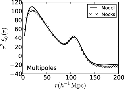
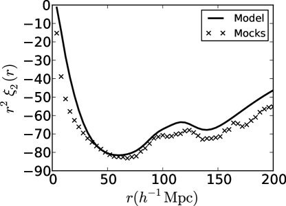
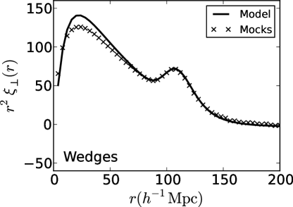
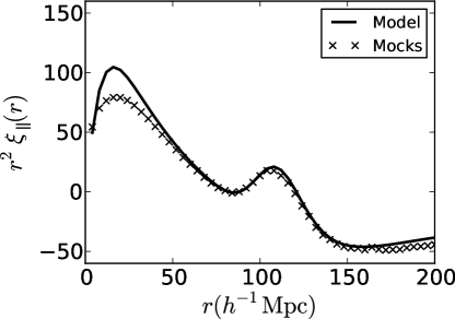
Figure 1 shows the average monopole and quadrupole and transverse and radial wedges of the correlation function over the 600 mocks (see § 4.2 for definitions).

Figure 1: Average of mocks (crosses) with our model of the correlation function (solid line) overplotted. The upper panels show the monopole (left) and quadrupole (right) while the lower panels plot the transverse (left) and radial (right) wedges. No fit to the shape was done here, but the models were normalized to match the observed signals.

3.5 Reconstruction

Following Anderson et al. (2012), we attempt to improve the statistical sensitivity of the BAO measurement by reconstructing the linear density field, correcting for the effects of non-linear structure growth around the BAO scale (Eisenstein et al., 2007a). The reconstruction technique has been successfully implemented on an anisotropic BAO analysis by Xu et al. (2013) using SDSS-II Luminous Red Galaxies at $z=0.35$, achieving an improvement of a factor of 1.4 on the error on $D_{A}$ and of 1.2 on the error on $H$, relative to the pre-reconstruction case. Anderson et al. (2012) successfully applied reconstruction on the same dataset used here when measuring $D_{V}$ from spherically-averaged two-point statistics. They observed only a slight reduction in the error of $D_{V}$, when compared to the pre-reconstruction case, but at a level consistent with mock galaxy catalogues.

The algorithm used in this paper is described in detail in Padmanabhan et al. (2012), to which we refer the reader for full details. Briefly, reconstruction uses the density field to construct a displacement field that attempts to recover a galaxy spatial distribution that more closely reproduces the expected result from linear growth. A summary of the implementation of the algorithm on the CMASS DR9 dataset (as used here) is given in Section 4.1 of Anderson et al. (2012).

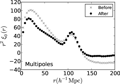
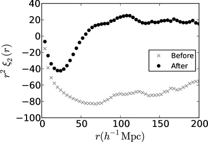
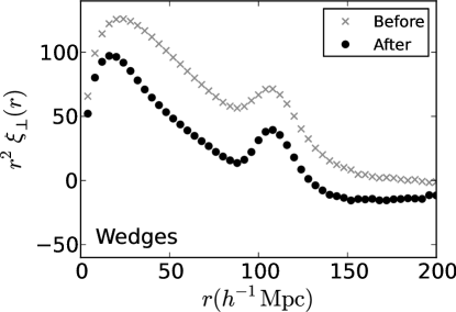
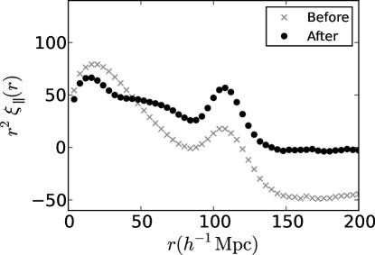
Figure 2 shows the average of the multipoles and wedges of the correlation function before and after reconstruction. Reconstruction sharpens the acoustic feature in the monopole, while decreasing the amplitude of the quadrupole, particularly at large scales where it goes close to zero. These changes are manifested in the wedges as a sharpening of the BAO feature in both wedges as well as a decrease in the difference in amplitude between the transverse and radial wedge. This is expected since reconstruction removes much of the large-scale redshift-space distortions. Assuming the correct cosmology, an ideal reconstruction algorithm would perfectly restore isotropy and eliminate the quadrupole In the wedges, this would be manifest by the transverse and radial wedge being the same. We depart from this ideal because of an imperfect treatment of of nonlinear evolution and small-scale effects, the survey geometry and imperfections in the implementation of the reconstruction algorithm itself. However, these imperfections affect the broad band shape of the correlation function but do not bias the location of the BAO feature, as we explicitly demonstrate below.

Figure 2: Average of mocks before (grey) and after (black) reconstruction. We see a sharpening of the acoustic feature in the monopole, and a drastic decrease in amplitude of the quadrupole on large scales, which is consistent with the fact that reconstruction removes large-scale redshift-space distortions. The correlation function of both angular wedges show a clear sharpening of the acoustic feature, a reduction of amplitude on large-scales in the transverse wedge and a corresponding increase in the amplitude in the radial wedge.

4 Method

4.1 Parametrization

The choice of an incorrect cosmology distorts the BAO feature in the galaxy correlation function, stretching it in both the transverse and radial directions. The shift in the transverse direction constrains the angular diameter distance relative to the sound horizon, $D_{A}(z)/r_{s}$, while the radial direction constrains the relative Hubble parameter $cz/(H(z)r_{s})$. As is standard in the BAO literature, when fitting for these, we parameterize with respect to a fiducial model (indicated by a superscript ${\rm fid}$) :

$$\alpha_{\perp}=\frac{D_{A}(z)r_{s}^{\rm fid}}{D^{\rm fid}_{A}r_{s}}\,,$$ (7)

and

$$\alpha_{||}=\frac{H^{\rm fid}(z)r_{s}^{\rm fid}}{H(z)r_{s}}\,.$$ (8)

An alternative parametrization is to decompose these shifts into isotropic and anisotropic components. We define an isotropic shift $\alpha$

$$\alpha=\alpha_{\perp}^{2/3}\alpha_{||}^{1/3}\,,$$ (9)

and the anisotropic shift $\epsilon$ by

$$1+\epsilon=\left(\frac{\alpha_{||}}{\alpha_{\perp}}\right)^{1/3}\,.$$ (10)

For the fiducial cosmological model, we have $\alpha=\alpha_{\perp}=\alpha_{\parallel}=1$ and $\epsilon=0$. For completeness, we note

$$\alpha_{\perp} =\frac{\alpha}{1+\epsilon}$$ (11)

$$\alpha_{||} =\alpha(1+\epsilon)^{2}\,\,.$$ (12)

The majority of previous BAO results have restricted their analysis to the isotropically averaged correlation function and have therefore presented their results in terms of $\alpha$. In this work, the fitting of the multipoles uses the $\alpha,\epsilon$ parametrization, while the clustering wedges use $\alpha_{||},\alpha_{\perp}$. While these are formally equivalent, the choices of data fitting ranges and priors imply that different parametrizations probe somewhat different volumes in model space, an issue we discuss in later sections. Although we use different parametrizations, we transform to the $\alpha_{\perp},\alpha_{||}$ parametrization when presenting results for ease of comparison.

4.2 Clustering Estimators : Multipoles and Wedges

Measuring both $D_{A}$ and $H$ requires an estimator of the full 2D correlation function $\xi(s,\mu)$ where $s$ is the separation between two points and $\mu$ the cosine of angle to the line of sight. However, working with the full 2D correlation function is impractical, given that we estimate our covariance matrix directly from the sample covariance of the mock catalogues. We therefore compress the 2D correlation function into a small number (2 in this paper) of angular moments and use these for our analysis.

The first set of these moments are the Legendre moments (hereafter referred to as multipoles) :

$$\xi_{\ell}(r)=\frac{2\ell+1}{2}\int_{-1}^{1}d\mu\,\xi(r,\mu)L_{\ell}(\mu)\,\,,$$ (13)

where $L_{\ell}(\mu)$ is the $\ell^{\rm th}$ Legendre polynomial. We focus on the two lowest non-zero multipoles, the monopole ($\ell=0$) and the quadrupole ($\ell=2$). Within linear theory and the plane-parallel approximation, only the $\ell=0,2$ and $4$ multipoles are non-zero. However, on these scales, the hexadecapole is both small and noisy; we neglect it in our analysis. Furthermore, after reconstruction, the effect of redshift space distortions is significantly reduced, further decreasing the influence of the hexadecapole.

We also consider an alternate set of moments, referred to as clustering wedges (Kazin et al., 2012):

$$\xi_{\Delta\mu}(r)=\frac{1}{\Delta\mu}\int_{\mu_{\rm min}}^{\mu_{\rm min}+\Delta\mu}d\mu\,\xi(r,\mu)\,,$$ (14)

For purposes of this study we choose $\Delta\mu=0.5$ such that we have a basis comprising of a “radial” component $\xi_{||}(s)\equiv\xi(\mu>0.5,s)$ and a “transverse” component $\xi_{\perp}(s)\equiv\xi(\mu<0.5,s)$. As the clustering wedges are an alternative projected basis of $\xi(\mu,\vec{s})$, we do not expect tighter constraints but rather find these useful for testing for systematics, as well as other technical advantages. A full in-depth description of the method, and comparison to clustering multipoles is described in Kazin et al. (2013).

4.3 A Model for the Correlation Function

Robustly estimating $D_{A}$ and $H$ from the correlation function requires a model for the 2D correlation function. We start with the 2D power spectrum template :

$$P_{t}(k,\mu)=(1+\beta\mu^{2})^{2}F(k,\mu,\Sigma_{s})P_{\rm dw}(k,\mu)$$ (15)

where

$$F(k,\mu,\Sigma_{s})=\frac{1}{(1+k^{2}\mu^{2}\Sigma_{s}^{2})^{2}}$$ (16)

is a streaming model for the Finger-of-God (FoG) effect (Peacock & Dodds, 1994) and the $(1+\beta\mu^{2})^{2}$ term is the Kaiser model for large-scale redshift-space distortions (Kaiser, 1987). Here $\Sigma_{s}$ is the streaming scale which we set to $1h^{-1}\rm{Mpc}$ based on test fits to the average mock correlation function. Note that there are currently two similar Lorentzian models for FoG in the literature. The difference arises from the following: 1) assuming that small-scale redshift space distortions can be modeled by convolving the density field with an exponential gives two powers of the Lorentzian in Fourier space as in Equation (16), 2) assuming that the pairwise velocity field is exponentially distributed results in only one power of the Lorentzian as in Hamilton (1998). We let $\beta$ vary in our fits (note that $\beta$ is degenerate with quadrupole bias). To limit the model from picking unphysical values of $\beta$, we place a Gaussian prior centered on $f/b\sim\Omega_{m}(z)^{0.55}/b=0.25$ before reconstruction and 0 after reconstruction with 0.2 standard deviation. The post-reconstruction prior center of $\beta=0$ is chosen since we expect reconstruction to remove large-scale redshift space distortions.

The de-wiggled power spectrum $P_{\rm dw}(k,\mu)$ is defined as

$$P_{\rm dw}(k,\mu)= [P_{\rm lin}(k)-P_{\rm nw}(k)]$$

$$\cdot\exp\bigg{[}-\frac{k^{2}\mu^{2}\Sigma_{\parallel}^{2}+k^{2}(1-\mu^{2})\Sigma_{\perp}^{2}}{2}\bigg{]}+P_{\rm nw}(k)$$

where $P_{\rm lin}(k)$ is the linear theory power spectrum and $P_{\rm nw}(k)$ is a power spectrum without the acoustic oscillations (Eisenstein & Hu, 1998). $\Sigma_{\parallel}$ and $\Sigma_{\perp}$ are the radial and transverse components of $\Sigma_{\rm nl}$, i.e. $\Sigma_{\rm nl}^{2}=(\Sigma_{\parallel}^{2}+\Sigma_{\perp}^{2})/2$, where $\Sigma_{\rm nl}$ is the standard term used to damp the BAO to model the effects of non-linear structure growth (Eisenstein et al., 2007b). Here, the damping is anisotropic due to the Kaiser effect. We set $\Sigma_{\perp}=6h^{-1}\rm{Mpc}$ and $\Sigma_{\parallel}=11h^{-1}\rm{Mpc}$ before reconstruction and $\Sigma_{\perp}=\Sigma_{\parallel}=3h^{-1}\rm{Mpc}$ after reconstruction as in Xu et al. (2013).

Given this model of the 2D power spectrum, we decompose it into its Legendre moments,

$$P_{\ell,t}(k)=\frac{2\ell+1}{2}\int^{1}_{-1}P_{t}(k,\mu)L_{\ell}(\mu)d\mu$$ (18)

which can then be transformed to configuration space using

$$\xi_{\ell,t}(r)=i^{\ell}\int\frac{k^{3}d\log(k)}{2\pi^{2}}P_{\ell,t}(k)j_{\ell}(kr).$$ (19)

Here, $j_{\ell}(kr)$ is the $\ell$-th spherical bessel function and $L_{\ell}(\mu)$ is the $\ell$-th Legendre polynomial. We then synthesize the 2D correlation function from these moments by :

$$\xi(r,\mu)=\sum_{\ell=0}^{\ell_{\rm max}}\xi_{\ell}(r)L_{\ell}(\mu)\,\,.$$ (20)

In this work, we truncate the above sum at $\ell_{\rm max}=4$.

In order to compare to data, we must map the observed $r_{\rm obs},\mu_{\rm obs}$ pairs (defined for a fiducial cosmology) to their true values $r,\mu$. These transformations are most compactly written by working in transverse ($r_{\perp}$) and radial ($r_{\parallel}$) separations define by

$$r^{2} =r_{\perp}^{2}+r_{\parallel}^{2}$$ (21)

$$\mu =\frac{r_{\parallel}}{r}$$ (22)

We then simply have

$$r_{\perp} =\alpha_{\perp}r_{\perp,{\rm obs}}$$ (23)

$$r_{\parallel} =\alpha_{\parallel}r_{\parallel,{\rm obs}}.$$ (24)

Expressions in terms of $r,\mu$ are in Xu et al. (2013) and Kazin et al. (2013). One can then compute $\xi(r,\mu)_{\rm obs}$ and project on to either the multipole or wedge basis.

Our final model for the correlation function includes nuisance parameters to absorb imperfections in the overall shape of the model due to mismatches in cosmology or potential smooth systematic effects. In particular, we fit

$$\xi_{0}(r) =B_{0}^{2}\xi_{0}(r)+A_{0}(r)$$

$$\xi_{2}(r) =\xi_{2}(r)+A_{2}(r)$$ (25)

and

$$\xi_{\perp}(r) =B_{\perp}\xi_{0,\perp}(r)+A_{\perp}(r)$$

$$\xi_{\parallel}(r) =B_{\parallel}\xi_{\parallel}(r)+A_{\parallel}(r)$$ (26)

where

$$A_{\ell}(r)=\frac{a_{\ell,1}}{r^{2}}+\frac{a_{\ell,2}}{r}+a_{\ell,3};\,\ell=0,2,\perp,\parallel\,.$$ (27)

Note that these correlation functions are all in observed coordinates; we just suppress the ${\rm obs}$ subscripts for brevity. The $A_{\ell}(r)$ marginalize errors in broadband (shape) information (eg. scale-dependent bias and redshift-space distortions) through the $a_{\ell,1}\ldots a_{\ell,3}$ nuisance parameters (Xu et al., 2012). $B_{0}^{2}$ is a bias-like term that adjusts the amplitude of the model to fit the data. We perform a rough normalization of the model to the data before fitting so $B_{0}^{2}$ should be $\sim 1$. To ensure $B_{0}^{2}$ is positive (a negative value would be unphysical), we perform the fit in $\log(B_{0}^{2})$ using a Gaussian prior with standard deviation 0.4 centered at 0 as described in Xu et al. (2012). While the multipole analysis does not include an analogous term for $\xi_{2}$, we allow $\beta$ to vary, effectively allowing the amplitude of the quadrupole to change. In the case of the wedges analyses, $\beta$ is kept fixed, but the amplitudes of both wedges are free to vary. No additional priors are imposed on these amplitudes. The clustering wedges analyses fit 76 data points with 10 parameters, while the multipole analyses fit 80 data points with 10 parameters.

We also place a 15% tophat prior on $1+\epsilon$ to limit low S/N measurements from exploring large excursions in $\epsilon$. Such a prior should have no impact for standard cosmological models. In order to demonstrate this, we sample cosmologies with $\Omega_{K}$, $w_{0}$ and $w_{a}$ free from the WMAP7 posterior distribution and compute $\epsilon$ for each case. The largest (absolute) excursion is $\sim$ 8% with 95% of points between$-0.058<\epsilon<0.045$, justifying the choice of our prior.

We assume a Gaussian likelihood for the correlation functions :

$$\chi^{2}=(\vec{m}-\vec{d})^{T}C^{-1}(\vec{m}-\vec{d})$$ (28)

where $\vec{m}$ is the model and $\vec{d}$ is the data. The inverse covariance matrix is a scaled version of the inverse of the sample covariance matrix $C_{s}$ (Muirhead, 1982; Hartlap et al., 2007)

$$C^{-1}=C^{-1}_{s}\frac{N_{\rm mocks}-N_{\rm bins}-2}{N_{\rm mocks}-1}$$ (29)

with the factor correcting for the fact that the inverse of the sample covariance matrix estimated from $N_{\rm mocks}$ is a biased estimate of the inverse covariance matrix.

The multipole and the clustering wedges analyses handle this likelihood surface differently. The wedges analysis uses a Markov Chain Monte Carlo algorithm to sample from the posterior distribution of $\alpha_{\perp}$ and $\alpha_{||}$, marginalizing over all the remaining parameters. The multipole analysis maps out the likelihood surface in $\alpha$ and $\epsilon$, analytically marginalizing over the linear parameters in the model, but using the maximum likelihood values for the non-linear parameters. In addition, to suppress unphysical downturns in the $\chi^{2}$ distribution at small $\alpha$ (corresponding to the BAO feature being moved to scales larger than the range of the data being fit, see Xu et al. (2012) for more details), we apply a Gaussian prior on $\log(\alpha)$ with a standard deviation of 0.15. As we see below, in the limit of a well detected BAO feature, these differences have a small (compared to our statistical errors) impact on the derived distances. However, in the opposite limit of a poorly measured BAO feature, these differences can be important. We explore this further in the next section. Fortunately, the DR9 sample has a well defined BAO feature and we obtain consistent results irrespective of the method.

5 Mock Results

5.1 Multipole Fits

Figure 3: A comparison of $\alpha_{\perp}$ and $\alpha_{\parallel}$ for the 600 mock catalogues before and after reconstruction. These values have been derived from the multipole analysis. The points mostly lie on the 1:1 line, but the number of outliers are reduced after reconstruction.

Figure 4: The distribution of $\alpha_{\perp}$ versus $\alpha_{\parallel}$ from the 600 mock catalogues after reconstruction. As in Fig. 3, these values are derived from the multipole analysis. The estimates of the two distances are anti-correlated, with a correlation coefficient of $\sim-0.44$. Note that $H\sim 1/\alpha_{||}$.

Figure 5: The errors in estimated distances, $\sigma_{\alpha_{\perp}}/\alpha_{\perp}$ versus $\sigma_{\alpha_{\parallel}}/\alpha_{\parallel}$, for the mock catalogues. The line of sight distance is more weakly constrained than the transverse distance.

Table 1: Fitting results from the multipole analysis of the mock catalogues for various parameter choices. The model is given in column 1. The median $\alpha_{\perp}$ is given in column 2 with the 16th/84th percentiles from the mocks given in column 3 (these are denoted as the quantiles in the text, hence the label Qtls in the table). The median $\alpha_{\parallel}$ is given in column 6 with corresponding quantiles in column 7. The median difference in $\alpha_{\perp}$ on a mock-by-mock basis between the model listed in column 1 and the fiducial model is given in column 4 with corresponding quantiles in column 5. The analogues for $\alpha_{\parallel}$ are given in columns 8 and 9. The mean $\chi^{2}$/dof is given in column 10.

Model	$\widetilde{\alpha_{\perp}}$	Qtls	$\widetilde{\Delta\alpha_{\perp}}$	Qtls	$\widetilde{\alpha_{\parallel}}$	Qtls	$\widetilde{\Delta\alpha_{\parallel}}$	Qtls	$\langle\chi^{2}\rangle/dof$
Redshift Space without Reconstruction
Fiducial $[f]$	$1.008$	${}^{+0.034}_{-0.037}$	–	–	$1.006$	${}^{+0.072}_{-0.074}$	–	–	60.06/70
$(\Sigma_{\perp},\Sigma_{\parallel})\rightarrow(8,8)h^{-1}\rm{Mpc}$.	$1.011$	${}^{+0.039}_{-0.038}$	$0.005$	${}^{+0.006}_{-0.006}$	$1.004$	${}^{+0.073}_{-0.088}$	$-0.007$	${}^{+0.012}_{-0.013}$	60.33/70
$\Sigma_{s}\rightarrow 0h^{-1}\rm{Mpc}$.	$1.007$	${}^{+0.035}_{-0.037}$	$0.000$	${}^{+0.000}_{-0.000}$	$1.006$	${}^{+0.071}_{-0.075}$	$-0.001$	${}^{+0.001}_{-0.001}$	60.04/70
$A_{2}(r)=poly2$.	$1.007$	${}^{+0.035}_{-0.037}$	$-0.000$	${}^{+0.002}_{-0.002}$	$1.008$	${}^{+0.071}_{-0.075}$	$0.001$	${}^{+0.006}_{-0.007}$	60.92/71
$A_{2}(r)=poly4$.	$1.007$	${}^{+0.035}_{-0.038}$	$0.000$	${}^{+0.003}_{-0.003}$	$1.010$	${}^{+0.070}_{-0.083}$	$-0.000$	${}^{+0.007}_{-0.007}$	59.20/69
$30<r<200h^{-1}\rm{Mpc}$ range.	$1.012$	${}^{+0.040}_{-0.038}$	$0.003$	${}^{+0.009}_{-0.007}$	$0.987$	${}^{+0.075}_{-0.090}$	$-0.017$	${}^{+0.014}_{-0.022}$	68.87/80
$70<r<200h^{-1}\rm{Mpc}$ range.	$1.007$	${}^{+0.033}_{-0.039}$	$-0.001$	${}^{+0.006}_{-0.007}$	$1.010$	${}^{+0.071}_{-0.075}$	$0.001$	${}^{+0.010}_{-0.012}$	52.28/60
$50<r<150h^{-1}\rm{Mpc}$ range.	$1.007$	${}^{+0.035}_{-0.037}$	$-0.001$	${}^{+0.008}_{-0.009}$	$1.010$	${}^{+0.073}_{-0.090}$	$0.000$	${}^{+0.017}_{-0.020}$	39.34/44
Redshift Space with Reconstruction
Fiducial $[f]$	$1.001$	${}^{+0.025}_{-0.026}$	–	–	$1.006$	${}^{+0.041}_{-0.045}$	–	–	61.06/70
$(\Sigma_{\perp},\Sigma_{\parallel})\rightarrow(2,4)h^{-1}\rm{Mpc}$.	$1.001$	${}^{+0.024}_{-0.027}$	$-0.001$	${}^{+0.001}_{-0.001}$	$1.007$	${}^{+0.040}_{-0.045}$	$0.001$	${}^{+0.002}_{-0.002}$	61.13/70
$\Sigma_{s}\rightarrow 0h^{-1}\rm{Mpc}$.	$1.001$	${}^{+0.025}_{-0.026}$	$0.000$	${}^{+0.000}_{-0.000}$	$1.006$	${}^{+0.041}_{-0.044}$	$-0.000$	${}^{+0.001}_{-0.001}$	60.99/70
$A_{2}(r)=poly2$.	$1.000$	${}^{+0.024}_{-0.026}$	$-0.001$	${}^{+0.001}_{-0.002}$	$1.006$	${}^{+0.043}_{-0.046}$	$-0.000$	${}^{+0.002}_{-0.001}$	63.40/71
$A_{2}(r)=poly4$.	$1.003$	${}^{+0.024}_{-0.026}$	$0.002$	${}^{+0.002}_{-0.003}$	$1.003$	${}^{+0.042}_{-0.046}$	$-0.003$	${}^{+0.004}_{-0.005}$	59.78/69
$30<r<200h^{-1}\rm{Mpc}$ range.	$1.004$	${}^{+0.025}_{-0.026}$	$0.003$	${}^{+0.004}_{-0.004}$	$1.008$	${}^{+0.040}_{-0.044}$	$0.000$	${}^{+0.006}_{-0.005}$	71.25/80
$70<r<200h^{-1}\rm{Mpc}$ range.	$1.002$	${}^{+0.023}_{-0.028}$	$-0.001$	${}^{+0.005}_{-0.004}$	$1.008$	${}^{+0.039}_{-0.044}$	$0.002$	${}^{+0.008}_{-0.007}$	52.48/60
$50<r<150h^{-1}\rm{Mpc}$ range.	$1.003$	${}^{+0.023}_{-0.026}$	$0.000$	${}^{+0.006}_{-0.006}$	$1.005$	${}^{+0.044}_{-0.047}$	$-0.002$	${}^{+0.009}_{-0.011}$	39.95/44

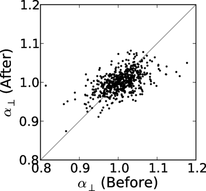
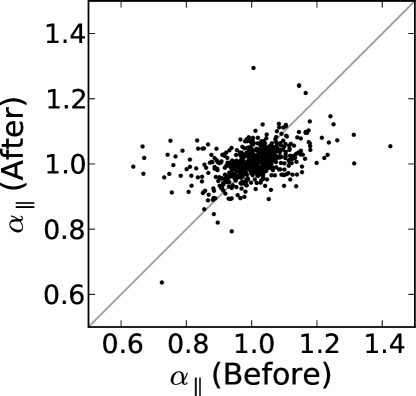
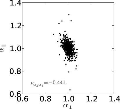
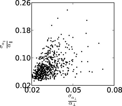
We start by summarizing the results of analyzing the multipoles measured from the mock catalogues; a corresponding discussion of the clustering wedges is in Kazin et al. (2013). A summary of multipole results is in Table 1 and in Figs. 3 to 5.

Figure 3 and the first line in Table 1 show that we recover the correct distances ($\alpha_{\perp}=\alpha_{\parallel}=1$) both before and after reconstruction. Reconstruction does reduce both the scatter in the measurements and the number of outliers, reflecting the sharpening of the acoustic signal in the correlation function.

Even though we measure both $\alpha_{\perp}$ and $\alpha_{\parallel}$, Figure 4 shows that these are correlated with a correlation coefficient of -0.441 (-0.494 before reconstruction). Note that the sign of this correlation reverses when we consider $D_{A}$ and $H$, since $H\sim 1/\alpha_{\parallel}$.

In Figure 5, we show the post-reconstruction $\sigma_{\alpha_{\perp}}/\alpha_{\perp}$ versus $\sigma_{\alpha_{\parallel}}/\alpha_{\parallel}$ values from each mock. The errors on $\alpha_{\perp}$ and $\alpha_{\parallel}$ are correlated as expected; the errors are related to the strength of the BAO signal in any given realization. Similar results are seen before reconstruction.

We also test the robustness of our fits by varying the fiducial model parameters; the results of these are in Table 1. We test cases in which $\Sigma_{\perp}$ and $\Sigma_{\parallel}$ are varied, $\Sigma_{s}$ is varied, the form of $A_{2}(r)$ is varied and the range of data used in the fit is varied. In general, the recovered values of $\alpha_{\perp}$ and $\alpha_{\parallel}$ are consistent with the fiducial model. The largest discrepancy arises in the pre-reconstruction measurement of $\alpha_{\parallel}$ where we have extended the fitting range down to $30h^{-1}\rm{Mpc}$. However, we know that our model at small scales is not particularly well matched to the mocks, as we saw in Figure 1, and hence the larger difference obtained by fitting down to smaller scales is not surprising. The smaller discrepancies in both $\alpha_{\perp}$ and $\alpha_{\parallel}$ when the other parameters are varied do not appear to be distinguishable in any individual mock as indicated by the quantiles on $\Delta\alpha_{\perp}$ and $\Delta\alpha_{\parallel}$. Xu et al. (2013) discuss similar differences and attribute them to disagreement between the model and data at small scales. In addition, the mock catalogues used here are derived from a perturbation theory based approach, so they may not be fully faithful on small scales.

5.2 Multipoles vs. Clustering Wedges

Figure 6: Comparison between the measurements (top rows) and estimated errors (bottom rows) for $\alpha_{\perp}$ and $\alpha_{||}$ obtained from the multipoles analysis and the corresponding results using the wedges technique, for all 600 PTHalos mocks. Left panels show the comparison before using reconstruction, and right panels show the comparison after reconstruction.

Figure 7: Same as Figure 6 but using the 100 groups of mocks, each of which is the average of six mocks, to increase the signal-to-noise ratio of the BAO feature. Note that in this case the agreement between the analysis using multipoles and wedges is much closer than in the non-stacked case.

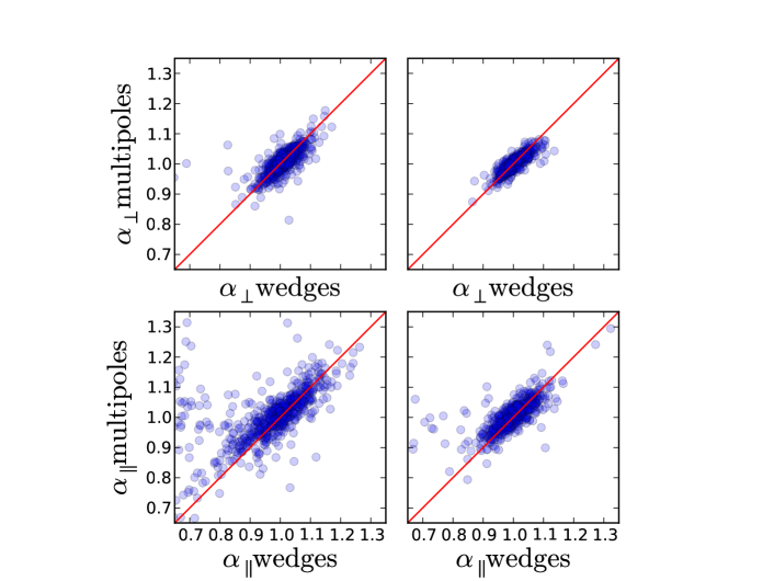
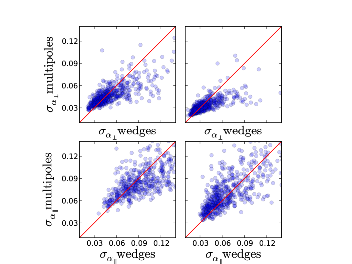
We now turn to comparisons of the results obtained in the previous section with the clustering wedges analysis in Kazin et al. (2013). In the limit where multipoles with $\ell\geq 4$ are negligible on large scales (as is our case), the monopole/quadrupole and clustering wedges are just a basis rotation and one would expect similar results from both. However, the marginalization of the broad band information and the various priors will impact the two differently. Furthermore, we adopt different techniques (and codes) in both, so this comparison tests the robustness of these approaches.

Figure 6 and Tables 2 and 3 summarize the results for both the measured distance scales and the estimated errors. Both methods yield identical results on average, but we note considerable scatter about this mean relation. Examining the individual mocks in detail, we find that a majority of these outliers correspond to realizations with a weak BAO detection. We quantify this by comparing fits with and without a BAO feature in them. Before reconstruction, 23% of the mocks have a $<3\sigma$ detection of the BAO feature in them; after reconstruction, this number drops to 4.6%. This improvement is also manifest in the right column of Figure 6.

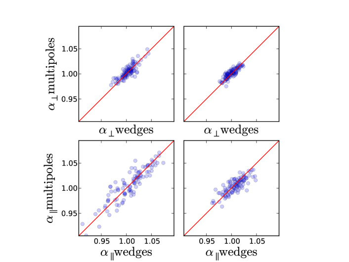
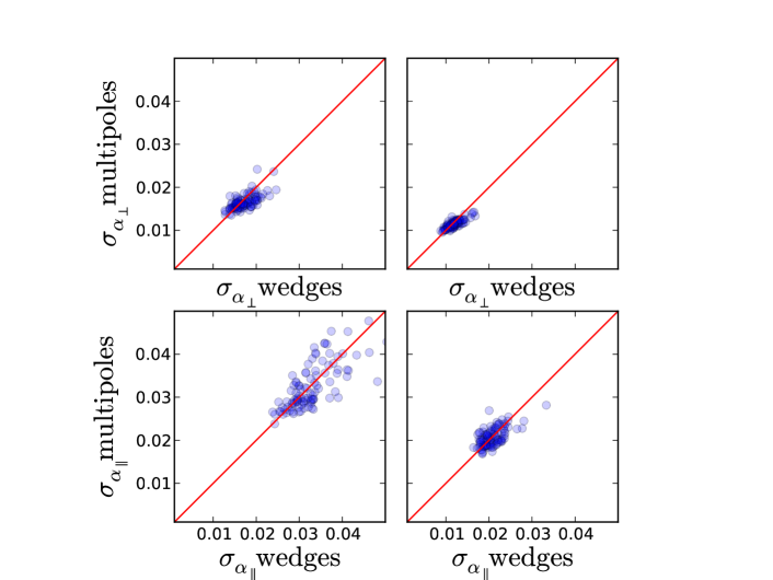
We further test this idea by recasting the mocks into 100 sets, each of which is the average of the correlation functions of 6 of our DR9 mocks. With an improvement in signal-to-noise ratio of a factor of $\sqrt{6}$, the acoustic peak is expected to be well detected. We present these results in Figure 7. There are none of the catastrophic failures of Figure 6 and very good agreement in both the estimated distances and errors for these individual “stacked” realizations. This suggests that the information content in these two approaches is indeed very similar.

Table 2: Average results from the 600 mocks (top four rows) and the 100 stacked mocks (bottow four rows). The table shows the median values of $\alpha_{\perp}$, $\alpha_{\parallel}$, $\sigma_{\alpha_{\perp}}$, and $\sigma_{\alpha_{\parallel}}$, together with their 68% confidence level region as shown by the 16^th and the 84^th percentiles in the mock ensemble. Results are shown for both multipoles and wedges, as well as pre- and post-reconstruction. As previously, tildes represent median quantities.

	$\widetilde{\alpha_{\perp}}$	$\widetilde{\alpha_{\parallel}}$	$\widetilde{\sigma_{\alpha_{\perp}}}$	$\widetilde{\sigma_{\alpha_{\parallel}}}$
	original mocks
wedges	$1.010^{+0.040}_{-0.040}$	$0.992^{+0.083}_{-0.124}$	$0.044^{+0.032}_{-0.012}$	$0.102^{+0.062}_{-0.033}$
multipoles	$1.008^{+0.035}_{-0.037}$	$1.007^{+0.070}_{-0.076}$	$0.044^{+0.016}_{-0.008}$	$0.088^{+0.041}_{-0.020}$
recon. wedges	$1.000^{+0.034}_{-0.027}$	$0.999^{+0.053}_{-0.052}$	$0.032^{+0.018}_{-0.009}$	$0.061^{+0.047}_{-0.018}$
recon. multipoles	$1.001^{+0.025}_{-0.026}$	$1.006^{+0.041}_{-0.045}$	$0.031^{+0.009}_{-0.005}$	$0.067^{+0.037}_{-0.017}$
	stacked mocks
wedges	$1.003^{+0.012}_{-0.012}$	$1.014^{+0.029}_{-0.038}$	$0.017^{+0.003}_{-0.002}$	$0.032^{+0.006}_{-0.004}$
multipoles	$1.004^{+0.013}_{-0.012}$	$1.010^{+0.033}_{-0.034}$	$0.016^{+0.002}_{-0.001}$	$0.031^{+0.008}_{-0.004}$
recon. wedges	$1.000^{+0.012}_{-0.010}$	$1.008^{+0.017}_{-0.020}$	$0.012^{+0.001}_{-0.001}$	$0.020^{+0.003}_{-0.002}$
recon. multipoles	$1.001^{+0.010}_{-0.009}$	$1.006^{+0.014}_{-0.016}$	$0.011^{+0.001}_{-0.001}$	$0.020^{+0.002}_{-0.002}$

Table 3: Average results from the 600 mocks (top two rows) and the 100 stacked mocks (bottow two rows). The table shows the median values of $\Delta\alpha_{\perp}$, $\Delta\alpha_{\parallel}$, $\Delta\sigma_{\alpha_{\perp}}$, and $\Delta\sigma_{\alpha_{\parallel}}$, (where $\Delta$ denotes the difference of the results using wedges minus the ones using multipoles) together with their 68% confidence level region as shown by the 16^th and the 84^th percentiles in the mock ensemble. Results are shown for both multipoles and wedges, as well as pre- and post-reconstruction. As previously, tildes represent median quantities.

	$\widetilde{\Delta\alpha_{\perp}}$	$\widetilde{\Delta\alpha_{\parallel}}$	$\widetilde{\Delta\sigma_{\alpha_{\perp}}}$	$\widetilde{\Delta\sigma_{\alpha_{\parallel}}}$
	original mocks
pre-recon.	$+0.004^{+0.020}_{-0.023}$	$-0.015^{+0.046}_{-0.053}$	$-0.000^{+0.019}_{-0.008}$	$+0.009^{+0.036}_{-0.019}$
post-recon.	$+0.001^{+0.015}_{-0.014}$	$-0.005^{+0.027}_{-0.027}$	$+0.000^{+0.011}_{-0.005}$	$-0.004^{+0.021}_{-0.016}$
	stacked mocks
pre-recon.	$-0.001^{+0.008}_{-0.007}$	$+0.001^{+0.014}_{-0.015}$	$+0.001^{+0.002}_{-0.002}$	$+0.000^{+0.003}_{-0.004}$
post-recon.	$-0.001^{+0.005}_{-0.006}$	$+0.003^{+0.007}_{-0.012}$	$+0.000^{+0.001}_{-0.001}$	$+0.000^{+0.002}_{-0.002}$

5.3 Isotropic vs anisotropic BAO measurements

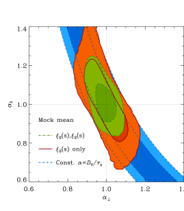
We now compare the results obtained from anisotropic BAO measurements with those derived from their isotropically averaged counterparts. As described in Section 4, spherically-averaged clustering measurements are only sensitive to the isotropic shift $\alpha$, while anisotropic measurements provide extra constraints on the distortion parameter $\epsilon$. Figure 8 compares the constraints on $\alpha_{\perp}$ and $\alpha_{\parallel}$ obtained by analyzing $\xi_{0}$ and $\xi_{2}$ (dot-dashed lines) with those obtained by analyzing $\xi_{0}$ alone (solid lines). To avoid noise from particular realizations, we use the average of the mock catalogues after reconstruction here. Analyzing the clustering wedges give essentially identical results.

As expected, the constraints derived from $\xi_{0}(s)$ exhibit a strong degeneracy well described by lines of constant $\alpha\propto D_{\rm V}/r_{\rm s}$, shown by the dashed lines; including $\xi_{2}$ breaks this degeneracy. The degeneracy is not perfect because large values of $\epsilon$ strongly distort the BAO feature in $\xi(s,\mu)$, causing a strong damping of the acoustic peak in the resulting $\xi_{0}(s)$. As the peak can be almost completely erased, these values give poor fits to the data when compared to $\epsilon=0$. We note that this requires going beyond the linear approximations used in Padmanabhan & White (2008) and Xu et al. (2013). However, these constraints are weak and can be ignored in all practical applications.

Figure 8: Comparison of the 65% and 95% constraints in the $\alpha_{\parallel}$–$\alpha_{\perp}$ plane obtained from the mean monopole of our mock catalogues (solid lines, orange), and from its combination with the mean quadrupole (dot-dashed lines, green). The constraints from $\xi_{0}(s)$ follow a degeneracy which is well described by lines of constant $\alpha\propto D_{\rm V}/r_{\rm s}$, shown by the dashed lines (blue). The extra information in the anisotropic BAO measurement helps to break this degeneracy.

6 DR9 Results

6.1 Basic Results

Figure 9: DR9 data (multipoles) before (top) and after (bottom) reconstruction with best-fit model (§ 4) overplotted. Note that the errors are correlated between bins. The distance parameters ($\alpha,\epsilon)$) of the best fit and the corresponding $\chi^{2}$ values are listed in the plots.

Figure 10: As in Figure 9 but for the clustering wedges.

Figure 11: The DR9 $\sigma_{D_{A}}/D_{A}$ and $\sigma_{H}/H$ values before (left) and after (right) reconstruction overplotted on the mock values. The DR9 values are consistent with the distribution expected from the mock catalogues, with the pre-reconstruction case on the better-constrained end and the post-reconstruction case more average.

Figure 12: Pre- and post-reconstruction 2D 68% contours and 1D probability distributions of $D_{A}$ and $H$ measured from the DR9 data, for both the multipoles and wedges. For consistency, both the multipoles and wedges have been analyzed with the MCMC code in Kazin et al. (2013). The lines mark the fiducial cosmology used in the analysis.

Table 4: DR9 fitting results for various models. The model is given in column 1. The measured $D_{A}(z)(r_{\rm s}^{\rm fid}/r_{\rm s})$ values are given in column 2 and the measured $H(z)(r_{\rm s}/r_{\rm s}^{\rm fid})$ values are given in column 3. The $\chi^{2}$/dof is given in column 4. For DR9 CMASS, $z=0.57$ and in our fiducial cosmology $r_{\rm s}^{\rm fid}=153.19$Mpc.

Model	$D_{A}(z)(r_{\rm s}^{\rm fid}/r_{\rm s})$	$H(z)(r_{\rm s}/r_{\rm s}^{\rm fid})$	$\chi^{2}/dof$
	(Mpc)	(km/s/Mpc)
Redshift Space without Reconstruction
Fiducial $[f]$	$1367\pm 44$	$86.6\pm 6.2$	43.29/70
$(\Sigma_{\perp},\Sigma_{\parallel})\rightarrow(8,8)h^{-1}\rm{Mpc}$.	$1371\pm 50$	$87.7\pm 5.8$	44.54/70
$\Sigma_{s}\rightarrow 0h^{-1}\rm{Mpc}$.	$1367\pm 44$	$86.7\pm 6.2$	43.26/70
$A_{2}(r)=poly2$.	$1366\pm 44$	$86.4\pm 6.1$	43.72/71
$A_{2}(r)=poly4$.	$1367\pm 44$	$86.6\pm 6.3$	43.29/69
$30<r<200h^{-1}\rm{Mpc}$ range.	$1357\pm 44$	$84.8\pm 5.7$	56.14/80
$70<r<200h^{-1}\rm{Mpc}$ range.	$1365\pm 44$	$86.5\pm 6.4$	41.68/60
Redshift Space with Reconstruction
Fiducial $[f]$	$1424\pm 43$	$95.4\pm 7.5$	53.29/70
$(\Sigma_{\perp},\Sigma_{\parallel})\rightarrow(2,4)h^{-1}\rm{Mpc}$.	$1419\pm 42$	$94.9\pm 7.6$	53.20/70
$\Sigma_{s}\rightarrow 0h^{-1}\rm{Mpc}$.	$1424\pm 43$	$95.6\pm 7.5$	53.34/70
$A_{2}(r)=poly2$.	$1422\pm 43$	$95.6\pm 7.8$	55.47/71
$A_{2}(r)=poly4$.	$1421\pm 43$	$94.9\pm 7.6$	52.76/69
$30<r<200h^{-1}\rm{Mpc}$ range.	$1433\pm 46$	$94.9\pm 8.2$	63.94/80
$70<r<200h^{-1}\rm{Mpc}$ range.	$1418\pm 40$	$95.4\pm 7.1$	42.92/60
$50<r<150h^{-1}\rm{Mpc}$ range.	$1405\pm 39$	$94.3\pm 6.4$	26.80/44

We now apply the methods validated in the previous section to the DR9 data. We assume the same fiducial cosmology as for the mock catalogs and use the same models and covariance matrices in our fits. As in the previous section, we begin by focusing on the multipole analysis and then compare with the companion analyses.

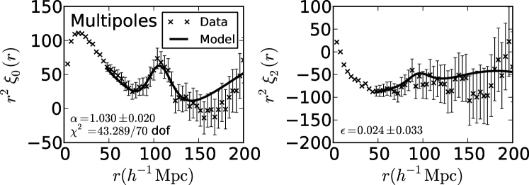
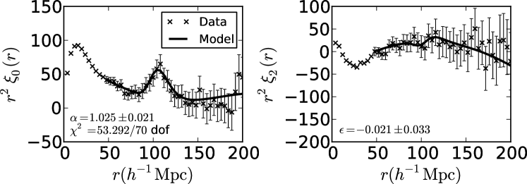
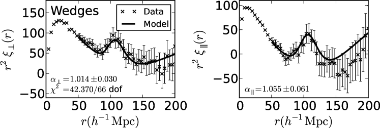
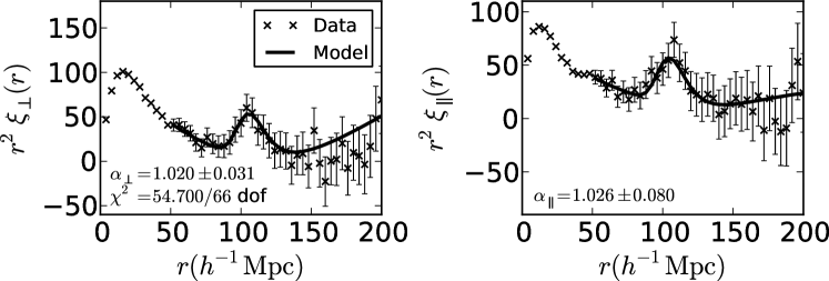
The DR9 data and the best-fit model (§ 4) are shown in Figures 9 for the multipoles and 10 for the wedges. Also shown are the best fit distance parameters, $\alpha,\epsilon$ for the multipoles and $\alpha_{\perp},\alpha_{\parallel}$ for the wedges, as well as the $\chi^{2}$-values of the fits. We remind the reader that although in most of the discussion we present $\alpha_{\perp,\parallel}$ results (to aid comparisons), the multipole analysis is done in $\alpha,\epsilon$ space. In all cases, the models are good fits to the data. As in Anderson et al. (2012), we do not see a significant improvement in the constraints after reconstruction. These measurements imply $D_{A}(z=0.57)=1367\pm 44\,{\rm Mpc}$ and $H(z=0.57)=86.6\pm 6.2\,{\rm km/s/Mpc}$ before reconstruction assuming a sound horizon equal to the fiducial value $r_{s}=153.19$ Mpc. After reconstruction we have $D_{A}(z=0.57)=1424\pm 43\,{\rm Mpc}$ and $H(z=0.57)=95.4\pm 7.5\,{\rm km/s/Mpc}$ : a 3.0% measurement of $D_{A}$ and a 7.9% measurement of $H$ at $z=0.57$. The two values are correlated with a correlation coefficient $\rho_{D_{A}H}=0.65$ before reconstruction and $\rho_{D_{A}H}=0.63$ after reconstruction. The difference from the expected value of $\rho_{D_{A}H}\sim 0.4$ (from the mocks) is due to sample variance. We also test the robustness of these results to variations in the choices made in the fitting procedure. The results are summarized in Table 4. Our results are insensitive to these choices, similar to the mock catalogues.

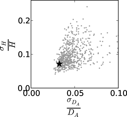
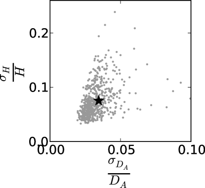
Figure 11 compares the DR9 $\sigma_{D_{A}}/D_{A}$ and $\sigma_{H}/H$ values from the multipole analysis with the distribution estimated from the mock catalogues. Before reconstruction, the DR9 data clearly lie towards the better constrained end of the mocks; after reconstruction, they appear more average. Indeed, our mock results indicate that $\sigma_{D_{A}}/D_{A}$ and $\sigma_{H}/H$ are actually larger after reconstruction $\sim 10\%$ of the time. We conclude that these measurements are consistent with our expectations.

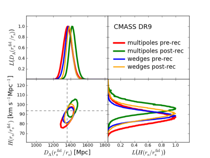
Figure 12 shows the 2D contours and marginalized 1D distributions in $\alpha_{\perp}$ and $\alpha_{\parallel}$ as measured by the wedges and multipoles. The likelihoods agree well before reconstruction but shift slightly after reconstruction. These differences are again consistent with the scatter seen in the mock catalogues: Figures 3 comparing the multipole measurements before and after reconstruction and Figure 6 comparing the multipoles and the wedges.

6.2 Consensus

The results on the mock catalogues demonstrate that both the multipoles and clustering wedges yield consistent results on average for $D_{A}$ and $H$. Furthermore, the mock catalogues do not favour one analysis technique over the other, either in terms of overall precision of the result or the robustness to outliers. In order to reach a consensus value appropriate for cosmological fits, we choose to average the log-likelihood surfaces obtained from both the clustering wedges and multipole measurements after reconstruction. As Figure 12 emphasizes, the core of these surfaces is very similar and this averaging will yield results consistent with either of the two individual approaches. Our consensus values are $H(0.57)=92.9\pm 7.8\,{\rm km/s/Mpc}$ and $D_{A}(0.57)=1408\pm 45{\rm Mpc}$ with a correlation coefficient of $0.55$. This correlation implies that using either value individually will yield sub-optimal constraints; using them together requires correctly accounting for the correlation between them.

Along with our statistical errors, we must also estimate any contribution from systematic errors. Systematic shifts in the acoustic scale are generally very small because the large scale of the acoustic peak ensures that non-linear gravitational effects are weak. Our analysis method uses the marginalization over a quadratic polynomial to remove systematic tilts from the measured correlation functions. The mock catalogs provide a careful check of the ability of the fitting method to recover the input cosmology. Table 1 shows this recovery to be better than 1%: after reconstruction, we find for the fiducial case a 0.1% shift in $\alpha_{\perp}$ and a 0.6% shift in $\alpha_{\parallel}$ using the multipole method. Other choices of fitting parameters vary the results by $O(0.2\%)$. The shifts in the wedges results are similar. Kazin et al. (2013) investigate the choice of fitting template (Eq. LABEL:eq:template) and find sub-percent dependence. Hence, we conclude that the systematic errors from the fitting methodology are small, of order 0.5%.

Beyond this, astrophysical systematic shifts of the acoustic scale are expected to be small. Mehta et al. (2011) showed that a wide range of halo occupation distribution galaxy bias models produced shifts of the acoustic scale of order 0.5% or less. Moreover, they found that the shifts vanished to within 0.1% after reconstruction was applied. It is likely that reconstruction in the DR9 survey geometry is less effective than it was in the Mehta et al. (2011) periodic box geometry, but we still expect the shifts from galaxy bias to be below 0.5%. The only astrophysical bias effect known to single out the acoustic scale is the early universe streaming velocities identified by Tseliakhovich & Hirata (2010). This effect can in principle be detected with enough precision to negligibly affect the final errors on the distance measurements (Yoo et al., 2011). However, we have not yet assessed this size of the signal in BOSS data, although it is not expected to be large given the vast difference in mass scale between CDM mini-halos and those containing giant elliptical galaxies.

We therefore estimate any systematic errors to be below 1%, which is negligible compared to our statistical errors. Future work will undoubtedly be able to further limit the systematic errors from both fitting methodology and galaxy bias.

6.3 Comparison with other Works

Figure 13: Pre-reconstruction joint likelihood distributions (68% confidence intervals) for $D_{A}(r_{s}^{\rm fid}/r_{s})$ and $H(r_{s}/r_{s}^{\rm fid}$) for different analyses of the CMASS DR9 data : multipole-based analyses (blue, this work, purple, Reid et al. (2012) and green, Chuang et al. (2013)) and the clustering wedges analysis (red, Kazin et al. (2013) and black, Sanchez et al. (2013)). This work and the companion work on wedges in Kazin et al. (2013) restrict to fitting the BAO position only, while the remaining works fit the full shape of the correlation function including the cosmological constraints from redshift-space distortions. All of these agree well, with the full-shape methods being generally more constraining than the BAO only methods.

Table 5: Summary of the measurements of $D_{\rm A}(z)(r_{s}^{\rm fid}/r_{\rm s})$, $H(z)(r_{\rm s}/r_{s}^{\rm fid})$, and their cross-correlation, $\rho_{D_{A}H}$, from the CMASS DR9 data. The upper and middle sections of the table list the values obtained in this work from the pre- and post-reconstruction analyses of multipoles and clustering wedges, respectively. Our consensus values, defined in Section 6.2, are also given. For comparison, the lower section of the table lists the results obtained in our companion papers, Kazin et al.(2013), Sánchez et al.(2013) and Chuang et al.(2013). All values correspond to the mean redshift of the sample, $z=0.57$.

	$D_{\rm A}(z)(r_{s}^{\rm fid}/r_{\rm s})$	$H(z)(r_{\rm s}/r_{s}^{\rm fid})$	$\rho_{D_{A}H}$
Before Reconstruction
$(\xi_{0}(s),\xi_{2}(s))$	$1367\pm 44$	$86.6\pm 6.2$	0.65
$(\xi_{\perp}(s),\xi_{\parallel}(s))$	$1379\pm 42$	$88.3\pm 5.1$	0.52
After Reconstruction
$(\xi_{0}(s),\xi_{2}(s))$	$1424\pm 43$	$95.4\pm 7.5$	0.63
$(\xi_{\perp}(s),\xi_{\parallel}(s))$	$1386\pm 36$	$90.6\pm 6.7$	0.50
Consensus	$1408\pm 45$	$92.9\pm 7.8$	0.55
Companion analyses
Kazin et al.	$1386\pm 39$	$90.3\pm 6.1$	0.48
Sánchez et al.	$1379\pm 39$	$91.0\pm 4.1$	0.30
Chuang et al.	$1371\pm 41$	$88.9\pm 6.1$	0.49
Reid et al.	$1395\pm 39$	$92.7\pm 4.5$	0.24

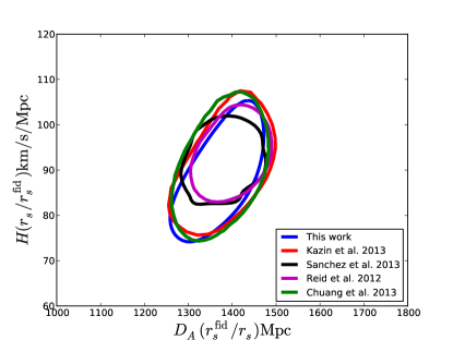
Figure 13 shows a comparison of the two-dimensional 68% confidence limits from our constraints on $D_{\rm A}(z)(r_{\rm s}^{\rm fid}/r_{\rm s})$ and $H(z)(r_{\rm s}/r_{\rm s}^{\rm fid})$ and those of our companion papers: Kazin et al. (2013), Chuang et al. (2013) and Sanchez et al. (2013) as well as the previous work by Reid et al. (2012). The corresponding one-dimensional marginalized constraints on these quantities are listed in Table 5 showing excellent consistency.

These analyses are based on different statistics and modelling details. Kazin et al. (2013) explore the geometric constraints inferred from the BAO signal in both clustering wedges and multipoles, by means of the de-wiggled template analysed here and an alternative form based on renormalized perturbation theory (Crocce & Scoccimarro, 2006). Chuang et al. (2013) and Sanchez et al. (2013) exploit the information encoded in the full shape of these measurements to derive cosmological constraints. While Kazin et al. (2013) and Chuang et al. (2013) follow the same approach applied here and treat $D_{\rm A}$ and $H$ as free parameters (i.e. without adopting a specific relation between their values), Sanchez et al. (2013) treats these quantities as derived parameters, with their values computed in the context of the cosmological models being tested. The consistency of the derived constraints on $D_{\rm A}(z=0.57)\left(r_{\rm s}^{\rm fid}/r_{\rm s}\right)$ and $H(z=0.57)\left(r_{\rm s}/r_{\rm s}^{\rm fid}\right)$ demonstrates the robustness of our results with respect to these differences in the implemented methodologies.

Reid et al. (2012) used the full shape of the monopole-quadrupole pair of the SDSS-DR9 CMASS sample to extract information from the Alcock-Paczynski test and the growth of structures. Based on these measurements they constrained the parameter combinations $D_{\rm V}(z)\left(r_{\rm s}^{\rm fid}/r_{\rm s}\right)=2072\pm 38\,{\rm Mpc}$ and $F(z)\equiv(1+z)D_{\rm A}(z)H(z)/c=0.675_{-0.038}^{0.042}$ at $z=0.57$. From our consensus anisotropic BAO measurements we infer the constraints $D_{\rm V}(z=0.57)\left(r_{\rm s}^{\rm fid}/r_{\rm s}\right)=2076\pm 58\,{\rm Mpc}$ and $F(z=0.57)=0.692\pm 0.087$, in excellent agreement with the results of Reid et al. (2012).

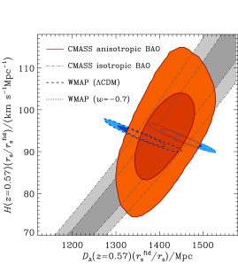
Anderson et al. (2012) studied the isotropic BAO signal using the same galaxy sample studied here. As discussed in Section 4, spherically-averaged BAO measurements constrain the ratio $D_{\rm V}(z)/r_{\rm s}$. By combining the results obtained from the post-reconstruction CMASS correlation function and power spectrum, Anderson et al. (2012) obtained a consensus constraint of $D_{\rm V}(z=0.57)\left(r_{\rm s}^{\rm fid}/r_{\rm s}\right)=2094\pm 33\,{\rm Mpc}$. This result corresponds to the constraints shown by the dot-dashed lines in Figure 14, which are in good agreement with the ones derived here. The comparison of these results illustrates the extra information provided by anisotropic BAO measurements, which breaks the degeneracy between $D_{A}$ and $H$ obtained from isotropic BAO analyses.

Assuming a flat $\Lambda$CDM cosmology, the information provided by CMB observations is enough to obtain a precise prediction of the values of $D_{\rm A}(z=0.57)\left(r_{\rm s}^{\rm fid}/r_{\rm s}\right)$ and $H(z=0.57)\left(r_{\rm s}/r_{\rm s}^{\rm fid}\right)$. The dashed lines in Figure 14 correspond to the predictions for these quantities derived under the assumption of a $\Lambda$CDM model from the WMAP observations of Bennett et al. (2012) (computed as described in Section 7). The anisotropic BAO constraints inferred from the CMASS sample are in good agreement with the $\Lambda$CDM WMAP predictions. This is a clear indication of the consistency between these datasets and their agreement with the standard $\Lambda$CDM model.

The CMB predictions are strongly dependent on the assumptions about dark energy or curvature. For any choice of $\Omega_{k}$ and $w(z)$, WMAP selects a different small region in the $D_{\rm A}(z=0.57)\left(r_{\rm s}^{\rm fid}/r_{\rm s}\right)$–$H(z=0.57)\left(r_{\rm s}/r_{\rm s}^{\rm fid}\right)$ plane. This is illustrated by the dotted contours in Figure 14, which correspond to the WMAP prediction obtained assuming a flat universe with dark energy equation of state parameter $w=-0.7$. If the assumptions about curvature and dark energy are relaxed, i.e., these parameters are allowed to vary freely, the region allowed by the CMB becomes significantly larger. Then, the combination of the CMB predictions with the BAO measurements can be used to constrain these cosmological parameters. In the next section we will explore the cosmological implications of the combination of these datasets.

Figure 14: Comparison of the 65% and 95% constraints in the $D_{\rm A}(z=0.57)\left(r_{\rm s}^{\rm fid}/r_{\rm s}\right)$–$H(z=0.57)\left(r_{\rm s}/r_{\rm s}^{\rm fid}\right)$ plane from the CMASS consensus anisotropic BAO constraints described in Section 6.2 (solid lines) and those of the isotropic BAO measurements of Anderson et al. (2012) (dot-dashed lines). The WMAP prediction for these parameters assuming a flat $\Lambda$CDM model (dashed lines), shows good agreement with the CMASS constraints. Note that the CMASS constraints do not assume $w=-1$ or flatness. The WMAP prediction obtained assuming a dark energy equation of state $w=-0.7$ is also shown (dotted lines).

7 Cosmological Implications

In this section we explore the constraints on the cosmological parameters in different cosmological models from an analysis of galaxy BAO and CMB data, highlighting the improvements obtained from the anisotropic multipole analysis of the BOSS DR9 CMASS galaxy sample introduced in this paper.

In Table 6 we summarize our main cosmological constraints for different cosmological models: $\Lambda$CDM in which the Universe is flat and dark energy is represented by a cosmological constant, $o$CDM in which the spatial curvature ($\Omega_{k}$) is a free parameter, $w$CDM in which we allow the equation of state of dark energy ($w$) to vary, and $ow$CDM in which we let both parameters vary. Different columns represent different combinations of CMB and BAO datasets. The CMB data comes from the final data release of WMAP (WMAP9; Hinshaw et al., 2012). We combine CMB data with BAO constraints from DR7 (SDSS-II LRGs) and DR9 (BOSS CMASS) galaxies. The isotropic BAO constraints include SDSS-II LRGs from Padmanabhan et al. (2012), and CMASS galaxies from Anderson et al. (2012), with anisotropic BAO data from SDSS-II LRGs in Xu et al. (2013) and from CMASS galaxies (this work).

As seen in Figure 14, the cosmological information contained in the anisotropic clustering data breaks the degeneracy present in the isotropic case between the angular diameter distance and the Hubble parameter (orange contours versus gray band respectively). Moreover, these distance measurements allow us to constrain cosmological parameters such as the spatial curvature $\Omega_{k}$ or the dark energy equation of state $w$. The blue contours in Figure 14 show CMB constraints assuming a $\Lambda$CDM model where we change the equation of state of dark energy to $w=-0.7$ from $w=-1$ (which is the case for a cosmological constant). We can see that the locus of the allowed parameter space is clearly different in each of these cases given the size of these error ellipses. We note that the distance constraints from the anisotropic BAO analysis are less tight and hence they benefit from the complementarity of other cosmological probes, such as the CMB. This complementarity allows for precision measurements of cosmological parameters. The allowed parameter space can could be further reduced by combining information from anisotropic clustering from surveys covering different redshift ranges: such as the low-redshift BAO measurements of the 6dF Galaxy Survey (Beutler et al., 2011) to the high-redshift Lyman $\alpha$ forest clustering results (Busca et al., 2012; Slosar et al., 2013; Kirkby et al., 2013).

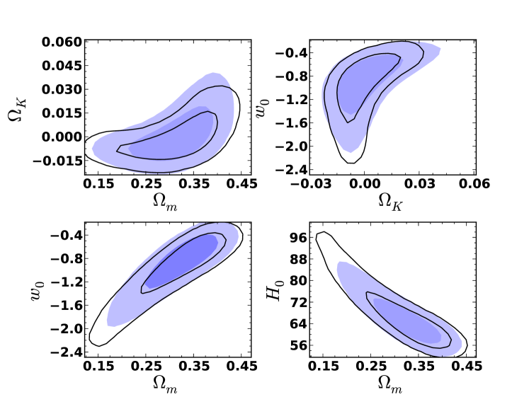
We find an improvement in the cosmological constraints in the $ow$CDM cosmological model from the anisotropic BAO analysis versus the spherically-averaged isotropic BAO analysis. These differences are apparent in Figure 15 where the BAO information is combined with CMB data. Plotted here are the likelihood contours of two cosmological parameters (from the set $\Omega_{k}$, $w$, $\Omega_{M}$, and $H_{0}$) while marginalizing over the remaining cosmological parameters in the $ow$CDM model. We can see that the allowed parameter space enclosed by the 68% and 95% confidence level contours is smaller in the anisotropic case, indicating that the anisotropic analysis provides a clear advantage in breaking the degeneracy between curvature and the equation of state of dark energy.

In Table 7 we compare cosmological constraints from the multipoles technique (this work) with the wedges technique discussed in §4. We find that the wedges analysis (Kazin et al., 2013) shows a marginally larger error bar in the cosmological parameters as compared to the multipoles technique. The table also compares the cosmological constraints using the consensus likelihood: the average of the log-likelihood from both multipoles and wedges. We find that both techniques show consistent results. When combined with CMB data, none of these results deviate significantly from a flat Universe with $\Omega_{k}=0.0$ or a cosmological constant with $w=-1$.

Figure 15: Constraints on the cosmological parameters of the $ow$CDM model when combining WMAP9 data with the anisotropic BAO data from CMASS presented in this work (filled blue contours). For comparison, the constrained parameter space from the combination of WMAP9 data with the isotropic BAO analysis in Anderson et al. (2012) is shown as black contours.

Table 6: Cosmological constraints from anisotropic BAO in CMASS DR9 data. Different rows show constraints on different cosmological models. Columns indicate different combinations of CMB and BAO datasets, where ’isotropic’ indicates the isotropic BAO analysis of Anderson et al. (2012), and ’anisotropic’ corresponds to the anisotropic BAO analysis presented here. The DR7 data include the analysis of the SDSS-II LRGs for the isotropic BAO in Padmanabhan et al. (2012) and the anisotropic results in Xu et al. (2013). The Hubble constant $H_{0}$ is in units of km s^-1 Mpc^-1.

Cosmological	Parameter	WMAP9	WMAP9	WMAP9	WMAP9	WMAP9
model		+DR9	+DR9	+DR7+DR9	+DR7+DR9
		(isotropic)	(anisotropic)	(isotropic)	(anisotropic)
$\Lambda$CDM
	$\Omega_{M}$	0.300$\pm$0.016	0.295$\pm$0.017	0.296$\pm$0.012	0.290$\pm$0.012	0.280$\pm$0.026
	$H_{0}$	68.3 $\pm$ 1.3	68.8 $\pm$1.4	68.7 $\pm$1.0	69.1$\pm$1.0	70.0 $\pm$2.2
$o$CDM
	$\Omega_{M}$	0.304$\pm$0.016	0.298$\pm$0.016	0.293$\pm$0.012	0.290$\pm$0.012	0.507$\pm$0.236
	$H_{0}$	67.1 $\pm$1.5	67.8 $\pm$1.7	68.2 $\pm$1.1	68.7$\pm$1.2	56.2 $\pm$12.4
	$\Omega_{k}$	-0.006 $\pm$0.005	-0.005$\pm$0.005	-0.004$\pm$0.005	-0.003$\pm$0.005	-0.056$\pm$0.060
$w$CDM
	$\Omega_{M}$	0.333$\pm$0.041	0.313$\pm$0.042	0.297$\pm$0.027	0.297$\pm$0.022	0.302$\pm$0.096
	$H_{0}$	64.5 $\pm$5.0	66.6 $\pm$5.6	68.5 $\pm$4.0	68.1$\pm$3.2	69.9 $\pm$11.5
	$w$	-0.84 $\pm$0.21	-0.90 $\pm$0.22	-0.99 $\pm$0.19	-0.95$\pm$0.15	-0.99 $\pm$0.35
$ow$CDM
	$\Omega_{M}$	0.310$\pm$0.070	0.314$\pm$0.058	0.269$\pm$0.045	0.284$\pm$0.039	0.596$\pm$0.254
	$H_{0}$	67.7 $\pm$9.6	66.7 $\pm$7.5	72.1 $\pm$6.7	69.7$\pm$5.3	51.9 $\pm$12.6
	$\Omega_{k}$	+0.000 $\pm$0.011	+0.002$\pm$0.013	-0.005$\pm$0.007	-0.002$\pm$0.008	-0.072$\pm$0.066
	$w$	-0.99 $\pm$0.44	-0.92 $\pm$0.37	-1.19 $\pm$0.34	-1.05$\pm$0.30	-1.02 $\pm$0.53

Table 7: Comparison of the cosmological constraints from the analysis of wedges, multipoles, and the consensus likelihood from both techniques, using anisotropic BAO CMASS DR9 data. Different rows show constraints on different cosmological models. The Hubble constant $H_{0}$ is in units of km s^-1 Mpc^-1.

Cosmological	Parameter	WMAP9+DR9	WMAP9+DR9	WMAP9+DR9
model		(consensus)	(multipoles)	(wedges)
$\Lambda$CDM
	$\Omega_{M}$	0.295$\pm$0.017	0.298$\pm$0.016	0.291$\pm$0.017
	$H_{0}$	68.8 $\pm$1.4	68.5 $\pm$1.3	69.1 $\pm$1.4
$o$CDM
	$\Omega_{M}$	0.298$\pm$0.016	0.301$\pm$0.016	0.296$\pm$0.019
	$H_{0}$	67.8 $\pm$1.7	67.5 $\pm$1.6	68.0 $\pm$2.0
	$\Omega_{k}$	-0.005$\pm$0.005	-0.005$\pm$0.005	-0.005$\pm$0.005
$w$CDM
	$\Omega_{M}$	0.313$\pm$0.042	0.326$\pm$0.033	0.307$\pm$0.043
	$H_{0}$	66.6 $\pm$5.6	64.9 $\pm$4.0	67.3 $\pm$5.8
	$w$	-0.90 $\pm$0.22	-0.84 $\pm$0.17	-0.93 $\pm$0.23
$ow$CDM
	$\Omega_{M}$	0.314$\pm$0.058	0.327$\pm$0.050	0.297$\pm$0.059
	$H_{0}$	66.7 $\pm$7.5	65.0 $\pm$6.2	69.0 $\pm$8.1
	$\Omega_{k}$	+0.002$\pm$0.013	+0.002$\pm$0.011	+0.000$\pm$0.011
	$w$	-0.92 $\pm$0.37	-0.85 $\pm$0.31	-1.03 $\pm$0.39

8 Conclusions

In this paper, we have presented a detailed analysis of the anisotropic measurement of the baryon acoustic peak in the SDSS-III BOSS DR9 sample of $0.43<z<0.7$ galaxies. The baryon acoustic oscillations provide a robust standard ruler by which to measure the cosmological distance scale. One of the important opportunities of the BAO method is its ability to measure the angular diameter distance and Hubble parameter separately at higher redshift. The BOSS DR9 sample is large enough to provide a detection of the acoustic peak both along and across the line of sight.

Our analysis has relied on two separate methods by which to measure the acoustic peak in the anisotropic correlation function. The first uses the monopole and quadrupole of the anisotropic clustering, following the methods of Xu et al. (2013). The second separates the correlation function into two bins of the angle between the separation vector of the pair and the line-of-sight, following Kazin et al. (2012). The latter analysis is further described in Kazin et al. (2013). In both cases, we fit a model of the correlation function to the data, using reconstruction to sharpen the acoustic peak and mock catalogs to define the covariance matrix of the observables. The fit is able to vary the position of the acoustic peak in both the line-of-sight and transverse directions, thereby measuring $H(z)$ and $D_{A}(z)$, respectively. The fitting includes a marginalization over broadband functions in both directions, thereby isolating the acoustic peak information from possible uncertainties in scale-dependent bias, redshift distortions, the reconstruction method, and systematic clustering errors.

From these fits, we define a consensus value of $H(0.57)(r_{s}/r_{s}^{\rm fid})=92.9\pm 7.8$ km/s/Mpc (8.4%) and $D_{A}(0.57)(r_{s}^{\rm fid}/r_{s})=1408\pm 45$ Mpc (3.2%). These two measurements have a correlation coefficient of 0.55 that should be taken into account when measuring parameters of cosmological models. We note that the sound horizon $r_{s}$ is constrained to $\sim$0.7% rms from current CMB data in simple adiabatic cold dark matter models (Bennett et al., 2012; Hinshaw et al., 2012); hence, the uncertainty in $r_{s}$ is subdominant for the usual fits.

Our results are highly consistent with the analysis of the spherically averaged acoustic peak in Anderson et al. (2012), which yielded a measurement of $D_{V}\propto D_{A}^{2/3}/H^{1/3}$. We find (Figure 8) that fitting the anisotropic model to only the monopole data returns constraints elongated in the $D_{V}$ direction, justifying the treatment in Anderson et al. (2012). We further find that when using the anisotropic data, we get constraints on $D_{V}$ similar to that of Anderson et al. (2012).

The cosmological parameter measurements we achieve from our measurement of $H(0.57)$ and $D_{A}(0.57)$ are similar to those found from $D_{V}(0.57)$ in Anderson et al. (2012). Because of those similarities, we have presented only a small sampling of cosmologies; further analyses can be found in Anderson et al. (2012). We find strong consistency with the standard flat $w=-1$ cosmological model. The fact that separating $D_{V}$ into separate $D_{A}$ and $H$ information does not improve the cosmological parameter fits is, we believe, largely due to the relatively low redshift of the data set: as $z\rightarrow 0$, $D_{A}$ and $H$ provide degenerate information in all cosmological models.

The analyses here and in Kazin et al. (2013) are focused only on the anisotropic acoustic peak. In addition, Reid et al. (2012), Sanchez et al. (2013), and Chuang et al. (2013) have studied the full shape of the anisotropic large-scale clustering in the BOSS DR9 CMASS sample. Such studies require more assumptions about the modeling of galaxy bias and redshift distortions, but offer stronger constraints on $H(z)$ through the use of the Alcock-Paczynski effect on the broadband clustering signal. The conclusions reached are consistent with those here from the acoustic peak alone.

The anisotropic measurement of the baryon acoustic oscillations has now been performed at three distinct redshifts: $z=0.35$ with the SDSS-II Luminous Red Galaxy sample, $z=2.3$ with the SDSS-III BOSS Ly$\alpha$ forest sample, and this analysis at $z=0.57$. All three have found strong consistency with the standard cosmological model of a spatially flat Universe with acceleration driven by a cosmological constant. These results represent only the first third of the SDSS-III BOSS data set but mark an important milestone for BAO studies. These anisotropic methods and measurements define a clear path for the ambitious surveys of the coming decade.

9 Acknowledgments

Numerical computations for the PTHalos mocks were done on the Sciama High Performance Compute (HPC) cluster which is supported by the ICG, SEPNet and the University of Portsmouth. Analyses were partially supported by were supported by facilities and staff of the Yale University Faculty of Arts and Sciences High Performance Computing Center.

We acknowledge the use of the Legacy Archive for Microwave Background Data Analysis (LAMBDA), part of the High Energy Astrophysics Science Archive Center (HEASARC). HEASARC/LAMBDA is a service of the Astrophysics Science Division at the NASA Goddard Space Flight Center.

Funding for SDSS-III has been provided by the Alfred P. Sloan Foundation, the Participating Institutions, the National Science Foundation, and the U.S. Department of Energy Office of Science. The SDSS-III web site is http://www.sdss3.org/.

SDSS-III is managed by the Astrophysical Research Consortium for the Participating Institutions of the SDSS-III Collaboration including the University of Arizona, the Brazilian Participation Group, Brookhaven National Laboratory, University of Cambridge, Carnegie Mellon University, University of Florida, the French Participation Group, the German Participation Group, Harvard University, the Instituto de Astrofisica de Canarias, the Michigan State/Notre Dame/JINA Participation Group, Johns Hopkins University, Lawrence Berkeley National Laboratory, Max Planck Institute for Astrophysics, Max Planck Institute for Extraterrestrial Physics, New Mexico State University, New York University, Ohio State University, Pennsylvania State University, University of Portsmouth, Princeton University, the Spanish Participation Group, University of Tokyo, University of Utah, Vanderbilt University, University of Virginia, University of Washington, and Yale University.

References

- Ahn et al. (2012) Ahn C. P. et al., 2012, ApJS, 203, 21
- Aihara et al. (2011) Aihara H. et al., 2011, ApJS, 193, 29
- Alcock & Paczynski (1979) Alcock C., Paczynski B., 1979, Nature, 281, 358
- Anderson et al. (2012) Anderson L. et al., 2012, MNRAS, 427, 3435
- Angulo et al. (2008) Angulo R. E., Baugh C. M., Frenk C. S., Lacey C. G., 2008, MNRAS, 383, 755
- Bennett et al. (2012) Bennett C. L. et al., 2012, ArXiv e-prints
- Beutler et al. (2011) Beutler F. et al., 2011, MNRAS, 416, 3017
- Blake et al. (2007) Blake C., Collister A., Bridle S., Lahav O., 2007, MNRAS, 374, 1527
- Blake et al. (2011a) Blake C. et al., 2011a, MNRAS, 415, 2892
- Blake & Glazebrook (2003) Blake C., Glazebrook K., 2003, ApJ, 594, 665
- Blake et al. (2011b) Blake C. et al., 2011b, MNRAS, 418, 1707
- Bolton et al. (2012) Bolton A. S. et al., 2012, AJ, 144, 144
- Bond & Efstathiou (1987) Bond J. R., Efstathiou G., 1987, MNRAS, 226, 655
- Busca et al. (2012) Busca N. G. et al., 2012, ArXiv e-prints
- Chuang & Wang (2012) Chuang C.-H., Wang Y., 2012, MNRAS, 426, 226
- Chuang et al. (2012) Chuang C.-H., Wang Y., Hemantha M. D. P., 2012, MNRAS, 423, 1474
- Chuang et al. (2013) Chuang C.-H., et al., 2013, MNRAS submitted
- Cole et al. (2005) Cole S. et al., 2005, MNRAS, 362, 505
- Crocce & Scoccimarro (2006) Crocce M., Scoccimarro R., 2006, Phys. Rev. D, 73, 063519
- Dawson et al. (2013) Dawson K. S. et al., 2013, AJ, 145, 10
- Doi et al. (2010) Doi M. et al., 2010, AJ, 139, 1628
- Eisenstein (2002) Eisenstein D., 2002, in Astronomical Society of the Pacific Conference Series, Vol. 280, Next Generation Wide-Field Multi-Object Spectroscopy, Brown M. J. I., Dey A., eds., p. 35
- Eisenstein & Hu (1998) Eisenstein D. J., Hu W., 1998, ApJ, 496, 605
- Eisenstein et al. (2007a) Eisenstein D. J., Seo H.-J., Sirko E., Spergel D. N., 2007a, ApJ, 664, 675
- Eisenstein et al. (2007b) Eisenstein D. J., Seo H.-J., White M., 2007b, ApJ, 664, 660
- Eisenstein et al. (2005) Eisenstein D. J. et al., 2005, ApJ, 633, 560
- Feldman et al. (1994) Feldman H. A., Kaiser N., Peacock J. A., 1994, ApJ, 426, 23
- Fukugita et al. (1996) Fukugita M., Ichikawa T., Gunn J. E., Doi M., Shimasaku K., Schneider D. P., 1996, AJ, 111, 1748
- Gaztañaga et al. (2009) Gaztañaga E., Cabré A., Hui L., 2009, MNRAS, 399, 1663
- Gunn et al. (1998) Gunn J. E. et al., 1998, AJ, 116, 3040
- Gunn et al. (2006) Gunn J. E. et al., 2006, AJ, 131, 2332
- Hamilton (1998) Hamilton A. J. S., 1998, in Astrophysics and Space Science Library, Vol. 231, The Evolving Universe, Hamilton D., ed., p. 185
- Hartlap et al. (2007) Hartlap J., Simon P., Schneider P., 2007, A&A, 464, 399
- Hinshaw et al. (2012) Hinshaw G. et al., 2012, ArXiv e-prints
- Hogg (1999) Hogg D. W., 1999, ArXiv Astrophysics e-prints
- Hu & Haiman (2003) Hu W., Haiman Z., 2003, Phys. Rev. D, 68, 063004
- Hu & Sugiyama (1996) Hu W., Sugiyama N., 1996, ApJ, 471, 542
- Huff et al. (2007) Huff E., Schulz A. E., White M., Schlegel D. J., Warren M. S., 2007, Astroparticle Physics, 26, 351
- Hütsi (2006) Hütsi G., 2006, A&A, 449, 891
- Hütsi (2010) Hütsi G., 2010, MNRAS, 401, 2477
- Jackson (1972) Jackson J. C., 1972, MNRAS, 156, 1P
- Kaiser (1987) Kaiser N., 1987, MNRAS, 227, 1
- Kazin et al. (2013) Kazin E., et al., 2013, MNRAS submitted
- Kazin et al. (2010) Kazin E. A. et al., 2010, ApJ, 710, 1444
- Kazin et al. (2012) Kazin E. A., Sánchez A. G., Blanton M. R., 2012, MNRAS, 419, 3223
- Kirkby et al. (2013) Kirkby D. et al., 2013, ArXiv e-prints
- Landy & Szalay (1993) Landy S. D., Szalay A. S., 1993, ApJ, 412, 64
- Lewis et al. (2000) Lewis A., Challinor A., Lasenby A., 2000, ApJ, 538, 473
- Linder (2003) Linder E. V., 2003, Phys. Rev. D, 68, 083504
- Lupton et al. (2001) Lupton R., Gunn J. E., Ivezić Z., Knapp G. R., Kent S., Yasuda N., 2001, in Astronomical Society of the Pacific Conference Series, Vol. 238, Astronomical Data Analysis Software and Systems X, Harnden Jr. F. R., Primini F. A., Payne H. E., eds., p. 269
- Manera et al. (2013) Manera M. et al., 2013, MNRAS, 428, 1036
- Mehta et al. (2012) Mehta K. T., Cuesta A. J., Xu X., Eisenstein D. J., Padmanabhan N., 2012, MNRAS, 427, 2168
- Mehta et al. (2011) Mehta K. T., Seo H.-J., Eckel J., Eisenstein D. J., Metchnik M., Pinto P., Xu X., 2011, ApJ, 734, 94
- Meiksin et al. (1999) Meiksin A., White M., Peacock J. A., 1999, MNRAS, 304, 851
- Miller et al. (2001) Miller C. J., Nichol R. C., Batuski D. J., 2001, ApJ, 555, 68
- Muirhead (1982) Muirhead R. J., 1982, Aspects of multivariate statistical theory, Wiley series in probability and mathematical statistics. Probability and mathematical statistics. John Wiley & Sons, New York
- Okumura et al. (2008) Okumura T., Matsubara T., Eisenstein D. J., Kayo I., Hikage C., Szalay A. S., Schneider D. P., 2008, ApJ, 676, 889
- Padmanabhan et al. (2008) Padmanabhan N. et al., 2008, ApJ, 674, 1217
- Padmanabhan et al. (2007) Padmanabhan N. et al., 2007, MNRAS, 378, 852
- Padmanabhan & White (2008) Padmanabhan N., White M., 2008, Phys. Rev. D, 77, 123540
- Padmanabhan & White (2009) Padmanabhan N., White M., 2009, Phys. Rev. D, 80, 063508
- Padmanabhan et al. (2012) Padmanabhan N., Xu X., Eisenstein D. J., Scalzo R., Cuesta A. J., Mehta K. T., Kazin E., 2012, MNRAS, 427, 2132
- Peacock & Dodds (1994) Peacock J. A., Dodds S. J., 1994, MNRAS, 267, 1020
- Peebles & Yu (1970) Peebles P. J. E., Yu J. T., 1970, ApJ, 162, 815
- Percival et al. (2007) Percival W. J., Cole S., Eisenstein D. J., Nichol R. C., Peacock J. A., Pope A. C., Szalay A. S., 2007, MNRAS, 381, 1053
- Percival et al. (2010) Percival W. J. et al., 2010, MNRAS, 401, 2148
- Perlmutter et al. (1999) Perlmutter S. et al., 1999, ApJ, 517, 565
- Pier et al. (2003) Pier J. R., Munn J. A., Hindsley R. B., Hennessy G. S., Kent S. M., Lupton R. H., Ivezić Ž., 2003, AJ, 125, 1559
- Reid et al. (2012) Reid B. A. et al., 2012, MNRAS, 426, 2719
- Riess et al. (1998) Riess A. G. et al., 1998, AJ, 116, 1009
- Ross et al. (2012) Ross A. J. et al., 2012, MNRAS, 424, 564
- Samushia et al. (2013) Samushia L. et al., 2013, MNRAS, 429, 1514
- Sanchez et al. (2013) Sanchez A., et al., 2013, MNRAS submitted
- Schlegel et al. (1998) Schlegel D. J., Finkbeiner D. P., Davis M., 1998, ApJ, 500, 525
- Scoccimarro & Sheth (2002) Scoccimarro R., Sheth R. K., 2002, MNRAS, 329, 629
- Seo et al. (2010) Seo H.-J. et al., 2010, ApJ, 720, 1650
- Seo & Eisenstein (2003) Seo H.-J., Eisenstein D. J., 2003, ApJ, 598, 720
- Seo & Eisenstein (2007) Seo H.-J., Eisenstein D. J., 2007, ApJ, 665, 14
- Seo et al. (2012) Seo H.-J. et al., 2012, ApJ, 761, 13
- Slosar et al. (2013) Slosar A. et al., 2013, ArXiv e-prints
- Smee et al. (2012) Smee S. et al., 2012, ArXiv e-prints
- Smith et al. (2002) Smith J. A. et al., 2002, AJ, 123, 2121
- Springel et al. (2005) Springel V. et al., 2005, Nature, 435, 629
- Sunyaev & Zeldovich (1970) Sunyaev R. A., Zeldovich Y. B., 1970, Ap&SS, 7, 3
- Swanson et al. (2008) Swanson M. E. C., Tegmark M., Hamilton A. J. S., Hill J. C., 2008, MNRAS, 387, 1391
- Tegmark et al. (2006) Tegmark M. et al., 2006, Phys. Rev. D, 74, 123507
- Tojeiro et al. (2012) Tojeiro R. et al., 2012, MNRAS, 424, 2339
- Tseliakhovich & Hirata (2010) Tseliakhovich D., Hirata C., 2010, Phys. Rev. D, 82, 083520
- Weinberg et al. (2012) Weinberg D. H., Mortonson M. J., Eisenstein D. J., Hirata C., Riess A. G., Rozo E., 2012, ArXiv e-prints
- Xu et al. (2013) Xu X., Cuesta A. J., Padmanabhan N., Eisenstein D. J., McBride C. K., 2013, MNRAS accepted
- Xu et al. (2012) Xu X., Padmanabhan N., Eisenstein D. J., Mehta K. T., Cuesta A. J., 2012, MNRAS, 427, 2146
- Yoo et al. (2011) Yoo J., Dalal N., Seljak U., 2011, JCAP, 7, 18