The Clustering of Galaxies in the SDSS-III Baryon Oscillation Spectroscopic Survey: Measuring and at with Clustering Wedges
Abstract
We analyze the 2D correlation function of the SDSS-III Baryon Oscillation Spectroscopic Survey (BOSS) CMASS sample of massive galaxies of the ninth data release to measure cosmic expansion and the angular diameter distance at a mean redshift of . We apply, for the first time, a new correlation function technique called clustering wedges . Using a physically motivated model, the anisotropic baryonic acoustic feature in the galaxy sample is detected at a significance level of compared to a featureless model. The baryonic acoustic feature is used to obtain model independent constraints ( accuracy) and () with a correlation coefficient of , where is the sound horizon scale at the end of the baryonic drag era. We conduct thorough tests on the data and 600 simulated realizations, finding robustness of the results regardless of the details of the analysis method. Combining with constraints from the Cosmic Microwave Background we obtain kms-1Mpc-1 and Mpc. We use simulations to forecast results of the final BOSS CMASS data set. We apply the reconstruction technique on the simulations demonstrating that the sharpening of the anisotropic baryonic acoustic feature should improve the detection as well as tighten constraints of and by on average.
keywords:
cosmological parameters, large scale structure of the universe, distance scale1 Introduction
One of the most exciting recent observations is the acceleration of the expansion of the Universe since redshift (Riess et al. 1998; Perlmutter et al. 1999). The origin of this phenomenon is thought to be an energy component with negative pressure (e.g, the so-called dark energy or a cosmological constant), or otherwise a break-down of General Relativity (Einstein 1916) on cosmic scales. For an in-depth summary of the observed acceleration and its possible interpretations, see Weinberg et al. (2012).
One method of measuring geometry from a 3D map of cosmological objects is through a geometric technique called the Alcock-Paczynski test (Alcock & Paczynski 1979) along with a standard ruler known as the baryonic acoustic feature. Alcock & Paczynski (1979) demonstrated that by assuming an incorrect cosmology when converting observed redshifts to comoving distances , a spherical cosmological body will appear deformed due to geometrical distortions. In the context of galaxy maps, this would cause a coherent distortion of the apparent radial positions and an anisotropic signature in clustering probes. Reproducing an isotropic clustering signal would result in obtaining the true cosmology. The observable of this process is , where is the expansion factor and is the angular diameter distance. To break this degeneracy, and hence improve constraining power, one can apply the technique on a standard ruler, such as the baryonic acoustic feature.
Early Universe plasma-photon waves propagated at close to the speed of sound from over dense regions, and came to a near halt at the era of decoupling of photons from baryons at at a characteristic comoving distance of Mpc from the originating over-density. This process left a distinctive signature in CMB anisotropies and in the large-scale structure of galaxies (Peebles & Yu 1970). Hu et al. (1997) review how the CMB anisotropies can be used to constrain fundamental cosmological parameters. Bassett & Hlozek (2010) review the baryonic acoustic signature in the clustering of matter and its usage as a standard ruler.
Following first baryonic acoustic feature measurements in the clustering of galaxies by Eisenstein et al. (2005) and Cole et al. (2005), two recent surveys, the WiggleZ Dark Energy Sky Survey (Drinkwater et al. 2010), and the Sloan Digital Sky Survey (SDSS-III; York et al. 2000; Eisenstein et al. 2011) Baryonic Oscillation Spectroscopic Survey (BOSS; Dawson et al. 2013), have reported detections of the baryonic acoustic feature at (Blake et al. 2011b, d; Anderson et al. 2012; Sánchez et al. 2012), as well as the 6dF Galaxy Survey (Jones et al. 2009) at (Beutler et al. 2011). Busca et al. (2012) and Slosar et al. (2013) also detect the baryonic acoustic feature, for the first time, in the Lyman-alpha forest of BOSS quasars between .
The focus of of most of these studies has been on the angle-averaged signal which constrains , where is the sound horizon at the end of the baryon drag era (see §2). This degeneracy originates because for every line-of-sight clustering mode (which constrains ), there are two transverse modes that constrain .
The subject of this study is breaking the degeneracy by using the Alcock-Paczynski effect through anisotropic clustering. This approach was first suggested by Hu & Haiman (2003) by using the two-dimensional power spectrum . Wagner et al. (2008) used mock catalogues at and 3 to demonstrate the usefulness of the technique. Shoji et al. (2009) argued that and information is encoded in the full 2D shape, and presented a generic algorithm that takes into account dynamic distortions on all scales, assuming all non-linear effects are understood. First attempts to apply these techniques on 2D and clustering planes were performed by Okumura et al. (2008), Chuang & Wang (2011), and Blake et al. (2011c).
Padmanabhan & White (2008) suggested decomposing the 2D correlation function into Legendre moments. They argue that the monopole ( angle averaged signal) and the quadrupole components (, see Equation 10) contain most of the relevant constraining information. Taruya et al. (2011) and Kazin et al. (2012) show that the hexadecapole term contains extra constraining power, which could be harnessed in the future with higher S/N than that currently available.
The advantage of analyzing 1D projections over the 2D plane is the relative simplicity of building a stable covariance matrix.
The first analyses of the anisotropic baryonic acoustic feature using and have been performed on the SDSS-II luminous red galaxy sample (; Xu et al. 2012a; Chuang & Wang 2012a, b) and the DR9-CMASS sample tested here (; Reid et al. 2012).
We analyze, for the first time, an alternative 1D basis suggested by Kazin et al. (2012), called clustering wedges . Gaztañaga et al. (2009) focused on a narrow clustering cylinder Mpc). In a subsequent analysis, Kazin et al. (2010) proposed using wider clustering wedges to improve S/N of the measurements. Kazin et al. (2012) analyzed the constraining power of and of on mock catalogues. They concluded that these statistics should be comparable in performance to the multipoles (, ) and provide a useful tool to test for systematics. The current study is the first analysis to perform such a thorough comparison on both data and mock galaxy catalogs.
Our analysis differs from the previous ones in a few other aspects. First, we compare results both before and after reconstruction. Reconstruction is a technique which corrects for the damping of the baryonic acoustic feature due to the large-scale coherent motions of galaxies. The baryonic acoustic feature is sharpened by calculating the displacement field and shifting galaxies to their near-original positions (Eisenstein et al. 2007a). Second, we follow a similar approach as in Xu et al. (2012a), by focusing on and and marginalizing over shape information. One notable difference from Xu et al. (2012a), however, is that they apply a linear approximation of the Alcock-Paczynski test, where here we use the full non-linear equations. We compare both methods in Appendix B, and show that the linear approach under-estimates the uncertainties of the obtained constraints. Finally, we compare between two independent theoretical templates.
This study is part of a series of papers analyzing the anisotropic clustering signal of the DR9 CMASS galaxy sample, containing massive galaxies between . Here we measure and in a model independent fashion through clustering wedges. Anderson et al. (2013) uses “consensus" values of clustering wedges and multipoles to infer cosmological implications. Both of these studies focus on the information contained within the anisotropic baryonic acoustic feature. Two further studies analyze the information from the full shape of : Sánchez et al. (2013) use the , and Chuang et al. (2013) focus on the multipoles .
This study is constructed as follows: in §2 we explain in detail the geometric information encoded in redshift maps. In §3 we define the clustering wedges and in §4 we present the data and mock catalogs. In §5 we describe the method used in our analysis; §6 describes our results. We discuss the results in §7 and summarize in §8.
To avoid semantic confusion, we briefly explain here the terminology of the different spaces mentioned throughout the text. First, all analyses are based on two-point correlation functions, which we refer to as configuration-space, as opposed to the Fourier domain called space. Second, when referring to a space affected by redshift distortions, we call it redshift space, and when there are none we refer to it as real space.
All the fiducial values calculated here are based on using the WMAP7 flat CDM cosmology (Komatsu et al. 2011). To calculate comoving distances we assume the matter density . Assuming this yields fiducial values: kms-1Mpc-1, Mpc at . Throughout, we also use derived unit-less relationships (, (, where Mpc (at ). For these we assume the baryon density , radiation density and photon density of .
2 Cosmic Geometry from Galaxy Maps
Although galaxy distributions in real-space are assumed to be statistically isotropic, measured clustering signals from galaxies from redshift maps are anisotropic. This is a result of two physical effects that are at play when converting observed redshifts to comoving distances :
| (1) |
The first, which we refer to as redshift-distortions, stems from the fact that is a degenerate combination of the cosmological flow and the radial component of the peculiar velocity. This results in anisotropic clustering components due to large-scale coherent flows (Kaiser 1987), and velocity dispersion effects within galaxy clusters. For a detailed introduction on dynamical redshift-distortions see Hamilton (1998).
On large scales, these effects can be used to test for deviations from General Relativity (Kaiser 1987; Linder 2008; see Guzzo et al. 2007; Samushia et al. 2012; Blake et al. 2011a; Samushia et al. 2013; Beutler et al. 2012 for the most recent measurements). The observable in this test is , where is the linear tracer to matter density bias, is the rate of change of growth of structure, is the linear growth of structure, and is the linear r.m.s of density fluctuations averaged in spheres of radii Mpc. This study focuses on a second more subtle effect which involves geometric distortions.
Comoving separations between two nearby points in space depend both on and the observer angle between them . Assuming the plane-parallel approximation between galaxy pairs, radial separations are defined as , where is the speed of light, and transverse distances , where the proper (physical) angular diameter distance is defined as:
| (2) |
where and is the representation of the curvature, and are the energy densities of compoenents X (matter, radiation, etc.).111Note that this is generic because . Hence, assuming an incorrect cosmology in Equation (1) would cause a spherical body (meaning ) to be deformed. For example, a lower than the true one would cause an elongation along the line-of-sight due to an increased , where a lower than the true value would cause a transverse squashing, because of a decrease of . Therefore, by fixing the observables and , retrieving a spherical shape constrains the combination.
Various techniques have been suggested to measure through this Alcock-Paczynski test (AP henceforth; Alcock & Paczynski 1979; Phillipps 1994; Lavaux & Wandelt 2012). Here we focus on clustering of galaxies, where line-of-sight clustering modes depend on () and transverse modes on (), and hence the anisotropies due the AP effect.
It has been pointed out that the anisotropies from this geometric effect are degenerate with those from redshift-effects (Ballinger et al. 1996). Various studies, such as Blake et al. (2011c) and Reid et al. (2012), show the degeneracy between and . In this study we marginalize over the redshift distortion information and focus on the geometric distortions.
In practice, when converting redshifts to comoving distances, the factors out trivially and thus we express comoving distance in units of Mpc, where ). The rest of the parameters in ( and their equation of states ) have more important, and potentially measurable, effects.
One way of overcoming these effects is to recalculate and then the clustering statistics for every set of parameters when determining cosmological constraints. However, that approach is currently not practical; instead, we vary a fixed clustering template, as described below.
Although the baryonic acoustic feature comoving scale is fixed, the apparent position measured in the correlation function depends on and . As demonstrated in Eisenstein et al. (2005), the baryonic acoustic feature in the angle average signal is sensitive, to first order, to . Padmanabhan & White (2008) show that analysis of the anistropic signal adds information, and hence breaks the degeneracy. To break the degeneracy with one needs to add additional information from the CMB anisotropies.
When relating measured from the CMB to that in the large-scale structure, one must take into account that these two definitions correspond to slightly different sound horizon radii (see Equation 1 in Blake & Glazebrook 2003). Because the baryons have momentum at decoupling , the baryonic acoustic signature in the distribution of matter is related to , where is the epoch when the baryonic drag effectively ended (Eisenstein & Hu 1998). The baryonic acoustic signature in the CMB anisotropies corresponds to . For current measurements see Hinshaw et al. (2012), and for predictions from the CMB, see Table 3 of Komatsu et al. (2009).
Conservation of the observer angle means that true separations transverse to the line-of-sight component will be related to an apparent “fiducial" component by:222Here we assume the plane-parallel approximation for each pair.
| (3) |
where
| (4) |
where the “f" subscript indicates the fiducial cosmology when calculating , and “t" indicates the true cosmology.
Similarly, the true line-of-sight separation component is related to the fiducial by:
| (5) |
with
| (6) |
The sound horizon terms appear due to the degeneracy with and , when applied to the baryonic acoustic feature as a standard ruler. Here we quote the rescaling in the position of the peak of the . The purely geometrical effect of changing the cosmology does not depend on .
In Appendix A we explain how we apply the AP test in practice through the mapping of between these coordinates systems.
3 Clustering Wedges
Assuming azimuthal statistical symmetry around the line-of-sight333The assumption of azimuthal statistical symmetry around the line-of-sight is true even with geometrical distortions. the 3D correlation function can be projected into 2D polar coordinates: the comoving separation and the cosine of the angle from the line-of-sight , where the line-of-sight direction is .
The 2D plane of can then be projected to clustering wedges as:
| (9) |
For the purpose of this study, we focus on two clustering wedges of , which we call line-of-sight and transverse . For consistency we compare all results to the multipole statistics defined as:
| (10) |
where are the standard Legendre polynomials.
The clustering wedges and multipoles are complementary bases of similar information. As shown by Kazin et al. (2012) up to order they are related by:
| (11) |
| (12) |
A useful relationship is the fact that the average of the clustering wedges results in .
In real space, where there are no anisotropies, all components are nulled, and clustering wedges of any width correspond to the monopole signal.444Homogeneity and isotropy are assumed here. The AP effect breaks this symmetry, causing components due to geometric distortions.
4 Data
We base our measurements of and on the large-scale anisotropic correlation function of the BOSS DR9-CMASS galaxy sample. Here we give a brief description of the sample, and the calculated .
4.1 The DR9-CMASS galaxy sample
We use data from the SDSS-III BOSS survey (Eisenstein et al., 2011; Dawson et al., 2013). The galaxy targets for BOSS are divided into two samples, LOWZ and CMASS. These are selected on the basis of photometric observations carried out with a drift-scanning mosaic CCD camera (Gunn et al., 1998, 2006) on the Sloan Foundation telescope at the Apache Point observatory. Spectra of these galaxies are obtained using the double-armed BOSS spectrographs (Smee et al., 2012). Spectroscopic redshifts are then measured by means of the minimum- template-fitting procedure described in Aihara et al. (2011), with templates and methods updated for BOSS data as described in Bolton et al. (2012).
Our analysis is based on the CMASS galaxy sample of SDSS Data Release 9 (DR9, Ahn et al. 2012). This sample was designed to cover the redshift ranges down to a limiting stellar mass, resulting on a roughly constant number density of (Eisenstein et al., 2011; Dawson et al., 2013, Padmanabhan et al. in preparation). This sample contains mostly central galaxies, with a satellite fraction (White et al., 2011; Nuza et al., 2012) and it is dominated by early type galaxies, although it contains a significant fraction of massive spirals (, Masters et al., 2011).
Anderson et al. (2012) present a detailed description of the construction of a CMASS catalogue for LSS studies. We follow the procedure detailed there and refer the reader to this article for more details.
4.2 PTHalo mock catalogues
Mock catalogues play a major role in the analysis and interpretation of large-scale structure information, as they offer a useful tool to test for systematics and provide the means with which to estimate statistical errors. In this analysis we use 600 PTHalo mock galaxy realizations to test our analysis pipeline and construct a covariance matrix of our measurements. Full details of the mock catalogues are given in Manera et al. (2012). Briefly, the mocks are based on dark matter 2LPT simulations ( order Lagrangian Perturbation Theory) , that were populated with mock galaxies within dark matter haloes. The halo occupation distribution (Peacock & Smith 2000; Seljak 2000; Scoccimarro et al. 2001; Berlind & Weinberg 2002; Cooray & Sheth 2002) parameters are determined by comparing the correlation function to that of the data in the scale range of Mpc.
To match the selection function of the data, the mock data is split by the Northern and Southern CMASS angular geometry and galaxies were excluded to match the radial profile.
4.3 The Anisotropic Correlation Function
To compute the correlation function, we use the Landy & Szalay (1993) estimator with an angular dependence:
| (13) |
We calculate the normalized data-data pair counts in bins of evenly separated and , , and similarly for data-random pairs, , and random-random, , where for each pair is defined as the direction in which a vector from the observer bisects . The values of each bin are the flat mean value. Our choice of binning is and Mpc.
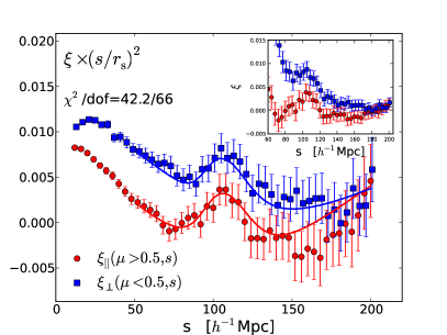
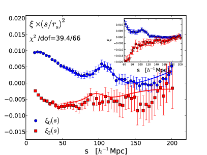
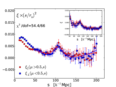
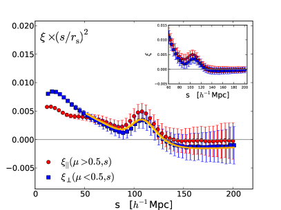
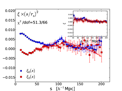
To obtain the clustering wedges we use Equation (9), where for we use the range [0,0.5] and for [0.5,1]. The resulting pre-reconstruction clustering wedges and multipoles are presented in top and bottom panels of Figure 1, respectively. The line-of-sight wedge is clearly weaker than the transverse wedge . This large difference in amplitudes on large-scales is due to redshift-distortions.
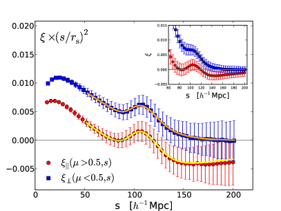
For comparison in the right panels of Figure 1 we show the mock-mean signals, i.e., the mean and of 600 mock catalogs.
4.4 Reconstructing the baryonic acoustic feature
Eisenstein et al. (2007a) showed that large-scale coherent motions, which cause a damping of the baryonic acoustic feature, can be ameliorated by using the gravitational potential estimated from the large-scale galaxy distribution to predict the bulk flows, and undo their non-linear effect on the density field. First studies focusing on periodic boxes shown that this reconstruction technique sharpens the baryonic acoustic feature, and hence improves its usage as a standard ruler (Padmanabhan et al. 2009; Noh et al. 2009; Seo et al. 2010; Mehta et al. 2011). We follow the procedure in Padmanabhan et al. (2012), which takes into account practical issues as edge effects by applying a Weiner filter (Hoffman & Ribak 1991; Zaroubi et al. 1995). We apply the reconstruction procedure on both the DR9-CMASS data, as well as on the mocks.
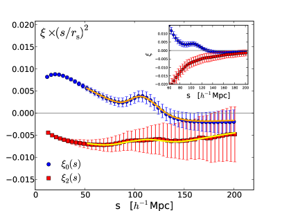
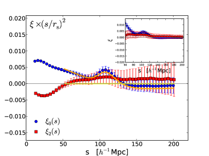
Figure 2 displays the post-reconstruction results for (top left) and the (bottom left). We clearly see that the amplitudes of the clustering wedges are aligned at the scales of the baryonic acoustic feature and larger. This is due to the fact that reconstruction not only corrects for large-scale coherent motions, but also corrects, to a certain extent, for redshift-distortions, as is seen by the near nullifying of the .
For comparison, the right panels Figure 2 show results of the post-reconstruction mock-mean signal. We clearly see that the reverses from negative at baryonic acoustic feature scales from the pre-reconstruction signal to positive. This change might be attributed to an over compensation of the redshift-distortions. In other words, throughout the reconstruction process, we estimate to shift galaxies in the radial direction, with the aim to reduce the Kaiser effect. An over-estimation could potentially put field galaxies a bit further away from high dense regions, and hence reverse the signal, yielding a that is slightly weaker than the . We are not concerned with this issue, because we do not expect redshift-distortions to shift the position of the anisotropic baryonic acoustic feature.
In both clustering wedges, in pre- and post-reconstruction, there is a clear signature of the baryonic acoustic feature. We quantify the significance of the detection in §6.1.
5 Analysis Methodology
5.1 Statistics used
When computing likelihoods of a model with a variable parameter space to fit data , we calculate the :
| (14) |
where are the bins tested. The likelihood is then assumed to be Gaussian
Throughout this analysis we run Monte Carlo Markov Chains (MCMC) nominally for nine or ten parameters as described in §5.3. We quote the mode of the posterior as our measurement and half the CL region (68CLr henceforth) for the uncertainty, because these are well defined regardless of asymmetries in likelihood profiles.
5.1.1 Covariance matrix
We construct the covariance matrix from the mock catalogues. (For a description of the mocks used see §4.2.) The signals are not independent but have significant cross-correlations. To take these correlations into account, when constructing the , we treat the mocks signals in an array of the form , meaning a 1D array with twice the length of the separation range of analysis. When analyzing the multipoles we apply a similar convention . We then construct a covariance matrix of defined as:
| (15) |
Figure 3 shows the correlation matrix of pre- and post-reconstrucion. The quartile has slightly larger (normalized) off-diagonal terms than in the quartile, demonstrated by the less steep gradient. There are also non-trivial positive and negative covariance cross-terms between the and . In the reconstructed we notice a sharper gradient, and a shallower negative region, indicating less dominance of the off-diagonal terms. This means that the reconstruction procedure reduces the covariance between the data points. Examining of the we find similar trends.
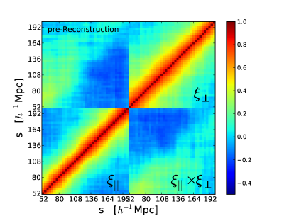
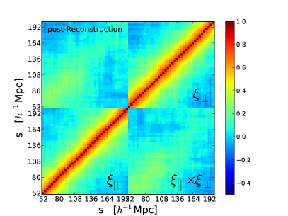
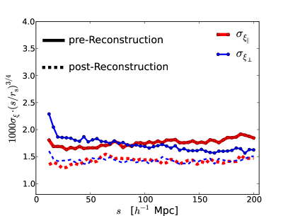
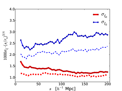
Figure 4 displays the square root of the diagonal elements. It is clear that pre-reconstruction the scatter in the two clustering wedges is slightly different, where post-reconstruction they are similar, and less than that of pre-reconstruction. We clearly see that yields the lowest scatter of all the statistics, and the highest, both pre- and post-reconstruction.
To correct for the bias due to the finite number of realizations used to estimate the covariance matrix and avoid underestimation of the parameter constraining region, after inverting the matrix to , we multiply it by the correction factors given in Hartlap et al. (2007):
| (16) |
In our analysis (238) (when analyzing region [50,200] Mpc), yielding a factor of .
5.2 Non-linear templates
The modeling is split into two parts: inclusion of redshift-distortions and modeling for non-linearities. Here we describe the former, and later consider two procedures for defining non-linearities.
Once the non-linear is defined (see §5.2.1), redshift-distortions are added such that the non-linear -space power spectrum is:
| (17) |
where .
| Template Name | Equation Base | Fixed parameter values | Comment |
|---|---|---|---|
| pre-rec | (18) | Mpc-1, , Mpc | |
| post-rec | (18) | Mpc-1, , Mpc | |
| pre-rec | (20) | Mpc, Mpc, Mpc | |
| post-rec | (20) | Mpc, Mpc | but small |
The dewiggled templates are shown in Figure 1 of Anderson et al. (2013).
After the base equation is calculated, Equation (17) includes redshift-distortions (post-rec assumes )
Although the velocity dispersion parameter appears to be an unresolved subject of investigation (Taruya et al. 2009), we find that applying it in the above Lorentzian format yields a good agreement with the mock-mean signals and down to Mpc. We find the Lorentzian format is preferred over the popular Gaussian.
The conversion to configuration space is accomplished by means of Equations (4.8) and (4.17) in Taruya et al. (2009). As described in Appendix A, we apply this calculation once to obtain the , templates, which are stored during the MCMC calculations. This approach means that we fix the parameters , , constant, and allow for their effective changes through the and shape parameters, as described in §5.3.1, §6.3.3. The values assumed for these parameters are summarized in Table 1.
5.2.1 Non-linear
We use two anisotropic templates. The primary focus is on a physically motivated model based on Renormalized Perturbation Theory (RPT), which takes into account first order corrections of mode coupling. Throughout this study we compare performance of this template to one that describes the effect of non-linearities in the baryonic acoustic feature through the “dewiggling" procedure. Both templates assume an exponential damping of the baryonic acoustic feature due to large-scale coherent motions, where in RPT-based this is assumed to be isotropic and in dewiggled anisotropic.
For the RPT-based template we write:
| (18) |
where
| (19) |
The mode coupling term is given by Equation (45) in Bernardeau et al. (2002). Pre-reconstruction we fix Mpc-1, which causes damping of the baryonic acoustic feature, and which takes into account mode coupling. These values are determined by analyzing the mean signal of the mocks whilst fixing and to the true values (and not using shape parameters). See §3 of Sánchez et al. (2013) for a thorough discussion of the template and a summary earlier investigations (e.g, Crocce & Scoccimarro 2008; Sánchez et al. 2008).
We compare the results obtained by means of the RPT-based model to a popular model denoted as dewiggled, which also includes a Gaussian damping of the baryonic acoustic feature:
| (20) |
where the anisotropic damping is defined by:
| (21) |
The is the no-wiggle model given in Eisenstein & Hu (1998). For a full description of this model, the reader is referred to Eisenstein et al. (2007b), Xu et al. (2012a), and §4.3 in Anderson et al. (2013). Here we use values Mpc for the pre-reconstruction case, and Mpc post-reconstruction.
5.2.2 Post-reconstruction templates
Equation (17) is used for both the RPT-based and dewiggled templates pre-reconstruction. Post-reconstruction templates are described in this section.
Assuming that the reconstruction procedure works correctly, one expects, in addition to the sharpening of the baryonic acoustic feature, a correction for redshift-distortions, yielding an isotropic . We apply this approach in the RPT-based modeling. Due to the sharpening of the baryonic acoustic feature, we set Mpc-1, which effectively yields the linear . The isotropy in the post-reconstruction template is introduced by setting and hence .
When applying reconstruction we also expect, ideally, no need for the coupling term. However, when analyzing the mocks, we find that setting to zero, yields a bias in . For this reason we fix as the pre-reconstruction template, which produces lower bias ( see Tables 2, 4).
For the dewiggled post-reconstruction template we assume an isotropic model, but do include Mpc contributions, which are small at the baryonic acoustic feature scale. This is the same template used in the analysis of Anderson et al. (2013).
As clearly seen in Figure 2, the reconstruction procedure, as applied on the PTHalos, yields a systematic effect in , which reverses sign at scales of the baryonic acoustic feature, suggesting there might be an over-compensation of the Kaiser effect. We are not concerned by this fact, as we are interested in the peak positions to extract and , and not . When using each of the templates, linear and non linear systematics of the reconstruction procedure are corrected by the shape parameters as described in §5.3.1. In §6.2 we demonstrate that for the RPT-based model the post-reconstruction results are essentially unbiassed.
5.3 The model tested
In this study we focus on the geometric information and contained in in a model-independent fashion. This is done by focusing on the information contained in the anisotropic baryonic acoustic feature, and hence marginalize over the shape effects, in a similar approach to that used in Xu et al. (2012a, b) and Anderson et al. (2012).
For each statistic analyzed we define a model based on a template using the following prescription:
| (22) |
where (,, or ). The and parameters are varied within by application of the non-linear AP effect, as described in §2 and Appendix A. In Appendix B, we also compare the non-linear to the linear AP shift and conclude that for DR9-CMASS the linear method underestimates constraints by , where is the 1D marginalized 68CLr of X=.555Results from tests on the DR9-CMASS pre-reconstructed .
5.3.1 The shape parameters
As indicated in Equation (22), each statistic “stat" is multiplied by its own independent amplitude factor . These factors take into account effective variations of , galaxy-to-matter linear bias, and the effective linear Kaiser boost.
For each clustering wedge model we add three additional non-linear parameters according to:
| (23) |
| (24) |
When testing for the we apply a similar approach. These terms are applied to the model only after the original template is shifted by the AP mapping. Hence, the parameter space used contains ten parameters:
| (25) |
where
| (26) |
where is the shape parameter for the statistic, as described in Equations (23,24).
In our analysis we find, however, that is not well constrained both pre- and post-reconstruction (this is not the case for the rest of ). We decide to fix this parameter, and hence are left with a nine parameter space , when analyzing . In Appendix C we verify that the results obtained with using yield similar results (modes and uncertainties) to those obtained with using both pre- and post-reconstruction. In §6.3.3 we describe degeneracies of the shape parameters with and constraints.
5.3.2 Priors
We limit and each to the region [0.5,1.5]. As suggested by Xu et al. (2012a), we test the effect of applying a Gaussian prior on the warping parameter . We also examine applying a flat prior on .
For most of this analysis, we do not use these priors, but we do examine using various prior values, and report a few results with flat prior . These priors are physically motivated. First, most reasonable cosmologies would find highly improbable. Second, the covariance matrix is limited to some extent, and reliability is questionable at high deviations from the fiducial cosmology (e.g, see Figures 16,17 in Samushia et al. 2012). Third, if the results yield a high , the fiducial cosmology should be revisited. Overall we find CMASS results are not sensitive to the choice of prior.
6 Results
In this section, we determine the significance with which the DR9-CMASS anisotropic baryonic acoustic feature is detected, and compare this to simulated realizations. We later describe the measurements of and .
6.1 Significance of the detection of the anisotropic baryonic acoustic feature
We generalize the standard technique of determining the significance of the detection of the baryonic acoustic feature to the 2D anisotropic case by usage of the clustering wedges, and apply this to the DR9-CMASS and the 600 mock realizations.
The method involves comparing the lowest result of a chosen physical model to a no-wiggle model. For a no-wiggle model we use the Eisenstein & Hu (1998) formalism (see their §4.2), and derive monopole and quadrupole components using of Equation (10).
Using this approach as a template, we run the same modeling and AP mapping (Equation 22) with the same parameter space as the physically motivated templates. In the procedure we do not attempt to analyze the clustering wedges separately from each other, i.e, we do not attempt to quantify significance of detection of the baryonic acoustic feature only in or . Instead, we quantify the significance of the detection of the anisotropic baryonic acoustic feature in the by using both . This is due to the co-variance between the clustering wedges, as well as the strong correlation between and . All the following results are similar when using the RPT-based or the dewiggled template.
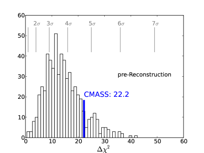
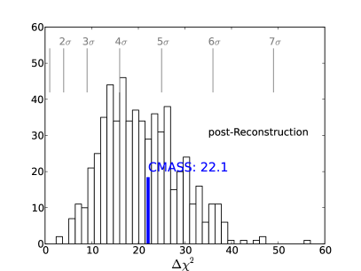
We apply this procedure on both the CMASS and the mock catalogs. The results are summarized in Figure 5, where the left panels correspond to pre-, and the right post-reconstruction. The top two panels correspond to the CMASS results as a function of and . The thick blue lines show the minimum surface of the RPT-based model compared to its minimum . The thin red line corresponds to the no-wiggle (no-peak) surface minimum model compared with . The bottom two panels are histogram results of the mock realizations, where the CMASS results are indicated with the thick vertical line. No priors on have been applied.
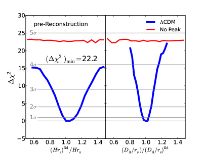
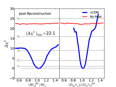
The pre-reconstruction CMASS clustering wedges yield a result of , meaning a 4.7 detection of the anisotropic baryonic acoustic feature, and we obtain a similar result after applying reconstruction. This result appears to be consistent with the isotropic baryonic acoustic feature detection of CMASS-DR9 as reported by Anderson et al. (2012), who showed a detection that did not improve with reconstruction.
In the pre-reconstruction case, the CMASS sample appears to be on the fortunate side of the mock distribution of the detection of the anisotropic baryonic acoustic feature, where of the mocks lie between . In the post-reconstruction case we see a clear shift of the mocks between .
For later reference we define a subsample of 462 realisations with a detection as the “ subsample", and its complement the “" subsample. For a consistent comparison between the various methods this subsample is defined when using the pre-reconstruction wedges RPT-based method. In the context of the DR9-CMASS volume, we find this separation useful for interpretation of the and results. For a visual of the subsamples in terms of , please see Figure 6.
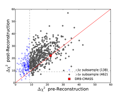
In the following section we analyze how well we expect to measure and both pre- and post-reconstruction.
6.2 Measuring , : testing methodology on mocks
To test the various assumptions made throughout
the analysis we first apply the pipeline to our mock catalogs.
To differentiate between systematic effects
and peculiarities due to mocks with low baryonic acoustic feature signal,
in Appendix C we investigate high
S/N mocks to answer the following questions (answers based on results in Table 4):
Does the method outlined in §5.3 affect the AP test?
The RPT-based result entries show that
the marginalization
over the shape information
yields small biases () in the geometric information measured.
Is one template preferred over the other?
We find that although the RPT-based and dewiggled templates
yield similar constraints and strong mode correlations,
the dewiggled one yields a bias in measuring (Appendix C.1).
The dewiggled template does not
have a mode coupling term, which might explain tendencies to yield more biased mock
results than the RPT-based template.
In §6.3.3 we report
results with varied , but
defer a more intensive investigation
of possible effects for future studies (e.g. the Taruya et al. 2010 model).
Is one combination preferred over the other?
We find that and
contain similar constraining power (Appendix C.2).
Are the resulting distributions of the and Gaussian?
We find that results of high S/N mocks
yield close to Gaussian (or symmetric)
posterior distributions but DR9-volume mocks do not.
This result is probably due to the fact
that the DR9 mock volumes contain a large fraction of
mocks with low S/N anisotropic baryonic acoustic feature.
Does reconstruction improve/bias the above?
We find that the reconstructed RPT-based template
yields a good description of the PTHalo mocks
and, on average, improves constraints of and by (Appendix C.3).
These tests show that the methods applied work well on high S/N mocks. Analyzing 600 PTHalo DR9-volumes, we find that a non-negligible amount of realizations yield low anisotropic baryonic acoustic feature signals.
Figure 7 shows correlations between and modes (top) and their uncertainties (bottom). As explained in Appendix C (and apparent in Figure 14), these distributions of and are not Gaussian. A visual inspection of various individual mocks reveals some cases with weak line-of-sight and/or transverse baryonic acoustic features. This is quantified in §6.1, where we find that of the realizations have an anisotropic baryonic feature with a significance of less than . For this reason, we separate the results to the subsample (gray points) and its complementary subsample (blue points) Note that in both pre- and post-reconstruction the subsamples are the same as that in pre-reconstruction (for a visual see Figure 6). This separation points to interesting trends in and modes and uncertainties.
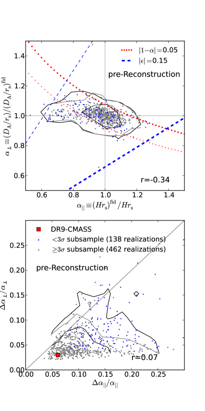
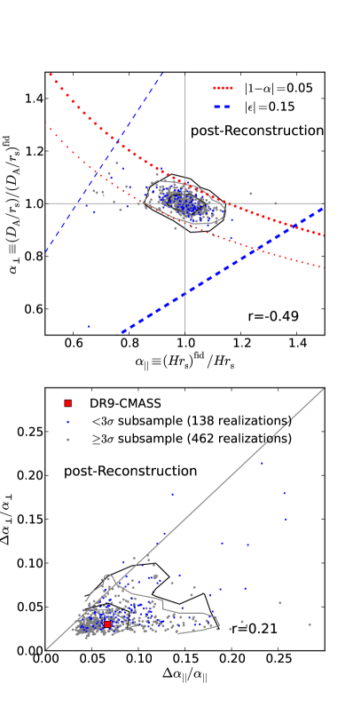
Most of the outliers that measure and modes at from the true values tend to be from the subsample in both pre- and post-reconstruction. The plot clearly shows that reconstruction substantially improves both mode and uncertainty scatters and constraints.
The uncertainty-uncertainty plots also show that most of the extremely large uncertainties are in the subsample. Although post-reconstruction removes the trend differences in the uncertainties, we clearly see that the tightest constraints are on the subsample.
For clarity of the plots and interpretation of results, we have applied a prior on the MCMC propositions. In the mode-mode plots this limit is shown by the dashed lines. The motivation behind this choice is given in §5.3.2. Without this prior, we find a systematic “pile-up" on the flat prior limit of =0.5, which is dominated by the subsample. We verify that these mocks have line-of-sight baryonic acoustic features that are either washed out, or contain a with a spurious strong clustering measurement at Mpc. For some of the “double-mode" realizations (meaning with both at line-of-sight baryonic acoustic feature signal and a spurious strong feature) the prior strengthens the true mode. For realizations with strong spurious features the prior causes them to move from closer to the boundary.
All the above trends appear in both templates examined (RPT-based, dewiggled), and in both clustering wedges and multipoles.
In Table 2 we summarize the mock results of and modes and uncertainties and their scatter. Most entries are for the RPT-based clustering wedges pre- and post-reconstruction. For completeness, the first and last entries include the dewiggled templates as well as including results of multipoles in all templates. The sample examined is indicated (e.g., full sample or the subsample) as well as if a prior on is used. For example, we investigate various priors, or restricting to realizations with and modes within from the true values, or both.
| ( of realizations) | / | / | ||
| Full sample, no priors: | ||||
| RPT-based wedges pre-Rec (600) | ||||
| RPT-based wedges post-Rec (600) | ||||
| RPT-based multipoles pre-Rec (600) | ||||
| RPT-based multipoles post-Rec (600) | ||||
| dewiggled wedges pre-Rec (600) | ||||
| dewiggled wedges post-Rec (600) | ||||
| dewiggled multipoles pre-Rec (600) | ||||
| dewiggled multipoles post-Rec (600) | ||||
| Full sample, : | ||||
| RPT-based wedges pre-Rec (600) | ||||
| RPT-based wedges post-Rec (600) | ||||
| subsample, no priors: | ||||
| RPT-based wedges pre-Rec (462) | ||||
| RPT-based wedges post-Rec (462) | ||||
| subsample, no priors: | ||||
| RPT-based wedges pre-Rec (208) | ||||
| RPT-based wedges post-Rec (208) | ||||
| subsample, no priors: | ||||
| RPT-based wedges pre-Rec (104) | ||||
| RPT-based wedges post-Rec (104) | ||||
| subsample, : | ||||
| RPT-based wedges pre-Rec (462) | ||||
| RPT-based wedges post-Rec (462) | ||||
| subsample, , : | ||||
| RPT-based wedges pre-Rec (394) | ||||
| RPT-based wedges post-Rec (450) | ||||
| RPT-based multipoles pre-Rec (374) | ||||
| RPT-based multipoles post-Rec (434) | ||||
| dewiggled wedges pre-Rec (392) | ||||
| dewiggled wedges post-Rec (445) | ||||
| dewiggled multipoles pre-Rec (371) | ||||
| dewiggled multipoles post-Rec (434) |
* The and columns show the median and rms of the modes.
* The and / columns show the median and rms of the fractional uncertainties.
Regarding the post-reconstruction RPT-based we notice that has in all cases a median mode bias of , and . Pre-reconstruction mode results, on the other hand, improve substantially when applying the various priors and cuts ( subsample, , mode limitation). These results show the effects of mocks with low anisotropic baryonic acoustic feature signal. For example when limiting the sample to the most constrained 2/3 of the realizations (meaning 394/600), the bias on improves from to , and of from to .
The and uncertainties improve in different manners when applying the various priors and cuts. The most noticeable trend, which is common for both parameter results, is the reduction of the scatter on the uncertainty when applying the prior.
For ill-constrained DR9 volumes the median uncertainties vary with choice of . On the other hand, for well-constrained realizations, such as CMASS-DR9, results do not depend on the prior (see §6.3).
We also find that the dewiggled pre-reconstruction template yields similar and constraints as the RPT-based ones, although the dewiggled pre-reconstruction template shows a systematic bias of on . This effect is not apparent in the high S/N mocks (Appendix C.2), which yield a median bias on , which is not apparent here. The post-reconstruction dewiggled wedges results are in line with the RPT-based.
Perhaps the most notable feature in Table 2 is that the scatter in the modes is different from the median of the uncertainties. Focusing on the most constrained subsample (the bottom entry), we see that the scatter in the modes is smaller than the median of the uncertainties in all cases. In §6.4 and Appendix C, we show that this should improve with higher S/N samples. For we see that the scatter of the modes and median of the uncertainties are fairly similar.
The fiducial cosmology of the analyses is the true cosmology of the mocks. We defer testing possible effects of using an incorrect fiducial cosmology (for preliminary tests on mocks see Kazin et al. 2012).
To summarize, we find that a significant minority of DR9-CMASS pre-reconstruction realizations yield unreliable results. However, the majority subsample yields a low bias result (). Moreover, the results show that the post-reconstruction wedges results yield low bias () with both RPT-based and dewiggled. We also find that for a DR9 volume we expect non-Gaussian likelihood profiles of and in both pre- and post-reconstruction. We next turn to apply the same method used here on the data both pre- and post-reconstruction.
6.3 DR9-CMASS , results
In this section we present our measurements of and in the DR9 CMASS dataset.
Our main pre- and post-reconstruction results are summarized in Figures 2 and 8. Post-reconstruction we measure ( accuracy; uncertainties are quoted at 68% CL) and ( accuracy). The correlation coefficient betwen and is measured at , similar to that predicted by Seo & Eisenstein (2007). The best fit model shows an excellent fit at dof= with dof=66 degrees of freedom. Compared to the mocks realizations, this result is better than 398/600 mocks. With the pre-reconstruction we obtain dof= (better than 578/600 realizations).
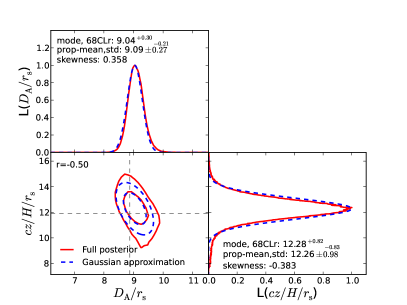
Figure 8 compares the posterior results (solid red lines) with a Gaussian approximation (dashed blue lines), based on the same quoted modes, uncertainties and cross-correlation coefficients. In both the pre- and post-reconstruction cases, we see that the Gaussian approximation describes the CL region fairly well, but clearly underestimates the CL reigon. We also note that the full posterior CL regions obtained both pre- and post-reconstruction are not well defined. These indicate the limited S/N in these measurement. We expect the agreement to improve with larger samples.
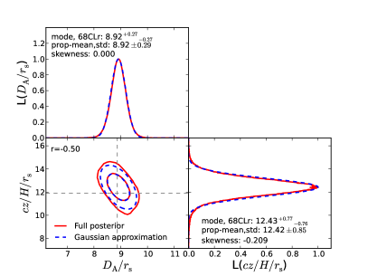
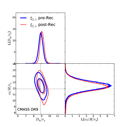
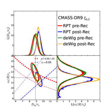
In the top plot of Figure 9 we show a direct comparison of the likelihood profiles pre- and post-reconstruction of the RPT-based clustering wedges. Both results appear to be similar, well within the CL region, although in the the post-reconstruction case is not as tightly constrained.
For an average mock DR9-volume realization we find a mode cross-correlation of , (or when examining the high S/N mocks; Appendix C.3) should be expected, where is the cross-correlation between the modes obtained when using one method (here pre-reconstruction) and when using a second (here post-reconstruction), and similar for , when discussing results. Also, although one does expect tighter constraints when applying reconstruction, the DR9 mocks indicate a (116/600) possibility of not improving . Using mocks with expected S/N of the final BOSS footprint (described in §6.4), this probability is reduced to .
The CMASS , results are summarized in Table 3 along with various related parameters.
6.3.1 Comparing results of various methods
The results quoted in the previous section are obtained when using the clustering wedges with the RPT-based template. Table 3 contains the results obtained for eight different combinations of statistics.
When applying the dewiggled template we obtain similar results to those obtained with RPT-based one. According to our mocks we expect , amongst the templates both pre- and post-reconstruction.
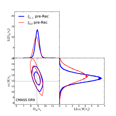
We apply the same test on the [,] multipoles and obtain slightly different results, but consistent within the CL regions, as seen in the bottom plot of Figure 9. According to the DR9 mock realizations we expect cross correlations between wedges results to multipoles by ,.
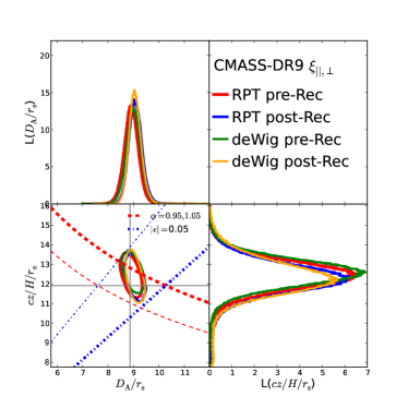
Figure 10 displays , likelihood profiles of all eight different methods analyzed here. The plot shows that all methods yield consistent results. The pre-rec (both RPT-based and dewiggled) profiles appear to be wider than the rest, where the post-rec (both RPT-based and dewiggled) appear to be the furthest from the rest, although clearly consistent within the CL regions. These differences are as expected based on the results from the mocks (for a visual of higher S/N mock results see top plot in Figure 12). We investigate various methods of shape parameters, and find similar results.
| No prior on : | kms-1Mpc-1 | Mpc | |||||
| RPT-based pre-Rec | 1.042 | 12.41 | 1.006 | 8.92 | -0.50 | 89.9 | 1367 |
| RPT-based pre-Rec | 1.072 | 12.77 | 0.989 | 8.77 | -0.72 | 87.4 | 1344 |
| dewig pre-Rec | 1.055 | 12.57 | 1.014 | 8.99 | -0.57 | 88.8 | 1378 |
| dewig pre-Rec | 1.070 | 12.74 | 1.008 | 8.94 | -0.72 | 87.5 | 1370 |
| RPT-based post-Rec | 1.031 | 12.28 | 1.020 | 9.05 | -0.51 | 90.8 | 1386 |
| RPT-based post-Rec | 0.974 | 11.60 | 1.055 | 9.36 | -0.67 | 96.2 | 1434 |
| dewig post-Rec | 1.026 | 12.22 | 1.020 | 9.05 | -0.54 | 91.3 | 1386 |
| dewig post-Rec | 0.974 | 11.60 | 1.046 | 9.28 | -0.62 | 96.2 | 1422 |
| prior : | |||||||
| RPT-based pre-Rec | 1.042 | 12.41 | 1.006 | 8.92 | -0.50 | 89.9 | 1367 |
| RPT-based pre-Rec | 1.072 | 12.77 | 0.989 | 8.77 | -0.75 | 87.4 | 1344 |
| dewig pre-Rec | 1.055 | 12.57 | 1.014 | 8.99 | -0.53 | 88.8 | 1378 |
| dewig pre-Rec | 1.070 | 12.74 | 1.008 | 8.94 | -0.72 | 87.5 | 1370 |
| RPT-based post-Rec | 1.031 | 12.28 | 1.020 | 9.05 | -0.50 | 90.8 | 1386 |
| RPT-based post-Rec | 0.974 | 11.60 | 1.052 | 9.33 | -0.78 | 96.2 | 1430 |
| dewig post-Rec | 1.026 | 12.22 | 1.020 | 9.05 | -0.53 | 91.3 | 1386 |
| dewig post-Rec | 0.974 | 11.60 | 1.046 | 9.28 | -0.63 | 96.2 | 1422 |
* We define and .
* Uncertainties quoted correspond to half of the marginalized CL region (68CLr). In parentheses is the mean percentage of 68CLr.
* All values are unitless, unless otherwise indicated.
* Fiducial values used at : (, (, based on WMAP5 cosmology (Komatsu et al. 2009).
* The , columns assume WMAP5 result: Mpc (Table 3 in Komatsu et al. 2009).
* is the cross-correlation coefficient for and .
6.3.2 Robustness of results to the range of fitted scales
As discussed in §5.3, these measurements focus on the information of the anisotropic baryonic acoustic feature and not from the full shape. As such, we do not expect dependency of our results on the range of scales used in the analysis.
The results quoted in the previous sections are obtained when analyzing data in the region of separations between . We compare the results obtained for various choices of . Figure 11 shows the comparison of the results.
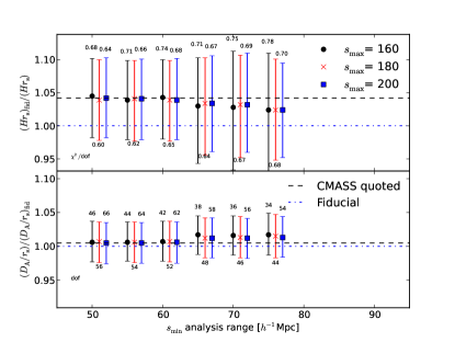
We find that, for the most part, the range of analysis does not affect our main results: mode values, uncertainties, cross-correlation coefficient or skewness. Regions of exception involve those with Mpc, in which the uncertainties increase from to and even higher, when limiting to =160 Mpc. This result could be explained by the fact that in this latter test the full dip of the baryonic acoustic feature is not used, and shape parameter values that cause spurious dips are accepted, whereas for lower values of they are not. We conclude that a more reliable result would include data points along the full shape, even though that information is marginalized over through the linear bias and terms.
We do not consider analyses with Mpc, because the templates used do not describe well the velocity-dispersion damping in the PTHalo mock-mean signal, and hence models would too heavily depend on the terms.
In all ranges investigated the is between , with the Mpc yielding the best fits, although not significantly better ones.
6.3.3 Regarding the nuisance and fixed parameters
As described in §5.3, we use a set of ten parameters . To best understand the effects and correlations of these parameters amongst themselves and with , we examine the results of both the data and the mock-mean signal. We perform these tests both pre- and post-reconstruction in both templates for and .
Overall, we do not see particular strong correlations between the shape parameters with , , where most cross-correlations are , but do illuminate a few findings of interest.
Most of the shape parameters have marginalized likelihood profiles that are fairly symmetric (low skewness). We find that amplitude parameters and are uncorrelated with each other. All correlations of these parameters with and are . The constant parameters () are uncorrelated to and , as expected. The other shape terms have weak correlations with and , (at ).
The most important finding of the shape parameters, however, regards the (the amplitude of the quadrupole). In both pre- and post-reconstruction its marginalized likelihood profile is not well constrained, causing strong skewness in the joint likelihoods with other parameters. We decide to fix its value, which yields results similar to , where this behaviour is not present.
We find all the above similar for the data and mock-mean in the pre-reconstruction case. In the post-reconstruction case this is true as well, after we apply a prior . Before applying the prior, the CL region is not well defined as the MCMC chains tend to accept values at the low limit set .
Finally we address the question of the parameter in the RPT-based template (Equation 18). Crocce & Scoccimarro (2008) introduced this parameterization to effectively take into account the coupling between the modes, which results in a shift in the peak position in . To obtain reliable templates of the post-reconstruction and we find that a model without an term yields biassed results in the mocks, by about in . When analyzing the post-reconstruction CMASS results, we see a shift in from 1.026 () to 1.030 (), a increase. The value is similar at . This results in a shift in and shift in , well below the uncertainties. For the post-reconstruction we find similar results.
6.4 Final CMASS Forecasts
By the conclusion of BOSS (2014), the survey will cover three times the area of the data set analyzed here, meaning The full CMASS sample will have a volume three times as large. By stacking the PTHalo mocks by groups of three, we can effectively, to first order, forecast the , results of the full CMASS galaxy sample. Using the 600 realizations, we analyze here results of 200 stacked mocks.
It is important to emphasize that the estimates yielded here should be considered maximum bounds. We argue this due to the fact that the used is the same DR9 volume covariance matrix as in Equation (15) but divided by three. This means that we do not account for noisy cross-correlations which should be reduced with the actual full CMASS geometry, thus we expect the constraining power to be tighter when using a more reliable . Furthermore, we note that replicating the DR9 geometry does not improve the reconstruction boundary effects.
Figure 12 displays the and results obtained by means of the expected modes and uncertainties, comparing between post- and pre-reconstruction (top), and post-reconstruction to (bottom).
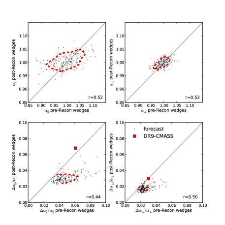
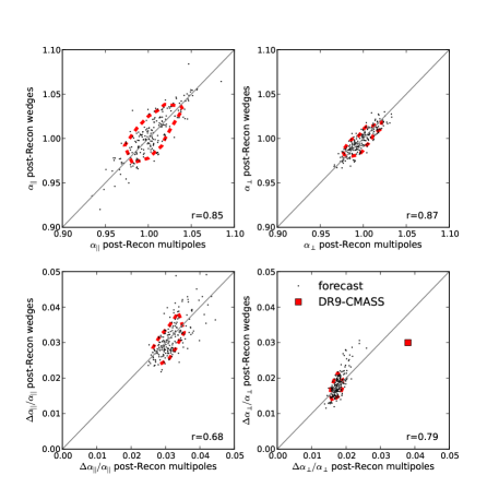
When comparing , results of the to the we find strong correlations where mode biases are sub . Uncertainties show that no method is preferred over the other. When comparing pre- and post-reconstruction wedges, we find a between the modes.
When applying reconstruction, the uncertainties are predicted to improve from to , a improvement. For the improvement is forecast to be from to , a improvement. The mock result distributions yield Gaussian-like features, although application the K-S tests indicates they are not Gaussian. These trends are similar to those seen with 100 six-stacked mocks (see Appendix C).
7 Discussion
The and results obtained here are consistent across the various techniques investigated:
-
1.
,
-
2.
template: RPT-based, dewiggled
-
3.
pre- and post-reconstruction
The likelihood profiles obtained with these eight combinations investigated, are shown in Figure 10 (as well as Figure 9 and Table 3). Differences between the results are as expected from mock simulations.
As these posteriors are not Gaussian, we provide joint 2D marginalized likelihood profiles of and , as well as provide the CMASS-DR9 and , on the World Wide Web.666http://www.sdss3.org/science/boss_publications.php We conclude this study by using results obtained post-reconstruction over those yielded pre-reconstruction, because we show that mock results expect an improvement of in the marginalized constraints of and , even though this is not the case in the data. We also prefer the RPT-based template over the dewiggled due to the larger bias in the mock results when using the latter. In the data, we find the posteriors to be similar regardless of choice of template (see Figure 10).
Comparison of our results to other analyses of the same data set can be found in the following studies. Anderson et al. (2013) measures and by applying a similar model-independent method on the , using the same dewiggled templates. The main differences in analysis involve their use of a grid of and , where the rest of the nuisance parameters are determined by the least-squares method. We perform extensive comparisons between the methods, and find the and results to be fairly similar (see Figures 13 and 14 in Anderson et al. 2013). Anderson et al. (2013) continue to use results obtained in both studies to produce a “consensus result" and calculate cosmological implications.
Model-dependent analyses are performed on the full shape of (Sánchez et al. 2013) and (Reid et al. 2012; Chuang et al. 2013). Sánchez et al. (2013) shows that results amongst these studies are compatible. Figure 15 in Sánchez et al. (2013) shows a comparison between our pre-reconstruction model independent result and their results from the full shape which are independent of parameter space, but assume follows GR predictions. They find an excellent agreement with our results, although tighter constraints as the baryonic acoustic feature only method effectively accepts parameter values (e.g, ) that the full shape does not.
8 Summary
In this study we investigate the ability of the BOSS DR9-CMASS volume to constrain cosmic geometry at , through the use of the AP technique applied on the anisotropic baryonic acoustic feature. We analyze the information contained in the anisotropic baryonic acoustic feature, for the first time, using a new technique called clustering wedges , and compare results to the multipoles .
We find the anisotropic baryonic acoustic feature to be detected in DR9-CMASS at a significance of compared to a featureless model (§6.1). We find this level to be fairly fortunate (from a cosmological variance perspective), but consistent with that expected from mock realizations. The application of reconstruction leads to a significant improvement of detection of the peak in mock catalogues from to (median standard deviations; see Figure 5). Pre-reconstruction mocks also show that (138/600) yield a detection lower than , whereas post-reconstruction do (28/600; Figure 6). Although we see clear improvement in the average mock realization, the significance of the detection of the anisotropic baryonic acoustic feature in the data does not improve after applying reconstruction. We find this, however, consistent with 89/600 () of the mock realizations (Figure 6).
To obtain geometrical constraints that are model independent, we use information from the post-reconstruction anisotropic baryonic acoustic feature and measure ( accuracy) and () with a correlation coefficient of (uncertainties are quoted at 68% CL). In terms of constraining and , the pre-reconstruction DR9-CMASS yields mutual constraints tighter than 584/600 of the mocks, putting it in the fortunate top . In the post-reconstruction case this is reduced to the top 444/600, meaning the top . Although CMASS-DR9 results do not improve with reconstruction, mock catalogs indicate that, on average, one should expect an improvement of constraining power of . Throughout this study we show that the posteriors of and from the DR9 volume are not expected to be Gaussian. In §7 we explain how to use the results presented here, pointing out that the provided full likelihood function should be used instead of a Gaussian approximation. Anderson et al. (2013) analyze cosmological consequences of this measurement.
In our analysis of mock catalogues we also demonstrate that the constraining power of and are expected to be similar. With this information we conclude that the analysis of the clustering wedges and comparison to the multipoles technique, as performed here, is vital for testing systematics when measuring and . Here we use wide clustering wedges of , which are fairly correlated (see Figure 3). As long as covariances can be adequately taken into account, this method could be generalized to narrower clustering wedges, as future surveys will yield better signal-to-noise ratio.
Acknowledgements
It is a pleasure to thank Chris Blake for his insight. Also we thank David Kirkby, Felipe Marin, Cameron McBride and Uros Seljak for useful discussions. EK is supported by the Australian Research Council Centre of Excellence for All-sky Astrophysics (CAASTRO), through project number CE110001020. AGS acknowledges support by the Trans-regional Collaborative Research Centre TR33 ‘The Dark Universe’ of the German Research Foundation (DFG). EK thanks Erin Sheldon for software used here. Numerical computations for the PTHalos mocks were done on the Sciama High Performance Compute (HPC) cluster which is supported by the ICG, SEPNet and the University of Portsmouth. Funding for SDSS-III has been provided by the Alfred P. Sloan Foundation, the Participating Institutions, the National Science Foundation, and the U.S. Department of Energy Office of Science. The SDSS-III web site is http://www.sdss3.org/. SDSS-III is managed by the Astrophysical Research Consortium for the Participating Institutions of the SDSS-III Collaboration including the University of Arizona, the Brazilian Participation Group, Brookhaven National Laboratory, University of Cambridge, Carnegie Mellon University, University of Florida, the French Participation Group, the German Participation Group, Harvard University, the Instituto de Astrofisica de Canarias, the Michigan State/Notre Dame/JINA Participation Group, Johns Hopkins University, Lawrence Berkeley National Laboratory, Max Planck Institute for Astrophysics, Max Planck Institute for Extraterrestrial Physics, New Mexico State University, New York University, Ohio State University, Pennsylvania State University, University of Portsmouth, Princeton University, the Spanish Participation Group, University of Tokyo, University of Utah, Vanderbilt University, University of Virginia, University of Washington, and Yale University.
References
- Ahn et al. (2012) Ahn C. P. et al., 2012, ApJS, 203, 21
- Aihara et al. (2011) Aihara H. et al., 2011, ApJS, 193, 29
- Alcock & Paczynski (1979) Alcock C., Paczynski B., 1979, Nature, 281, 358
- Anderson et al. (2012) Anderson L. et al., 2012, MNRAS, 427, 3435
- Anderson et al. (2013) Anderson L. et al., 2013, ArXiv e-prints
- Ballinger et al. (1996) Ballinger W. E., Peacock J. A., Heavens A. F., 1996, MNRAS, 282, 877
- Bassett & Hlozek (2010) Bassett B., Hlozek R., 2010, Baryon acoustic oscillations, Ruiz-Lapuente P., ed., p. 246
- Berlind & Weinberg (2002) Berlind A. A., Weinberg D. H., 2002, ApJ, 575, 587
- Bernardeau et al. (2002) Bernardeau F. et al., 2002, Phys. Rep., 367, 1
- Beutler et al. (2011) Beutler F. et al., 2011, MNRAS, 416, 3017
- Beutler et al. (2012) Beutler F. et al., 2012, MNRAS, 423, 3430
- Blake et al. (2011a) Blake C. et al., 2011a, MNRAS, 415, 2876
- Blake et al. (2011b) Blake C. et al., 2011b, MNRAS, 415, 2892
- Blake & Glazebrook (2003) Blake C., Glazebrook K., 2003, ApJ, 594, 665
- Blake et al. (2011c) Blake C. et al., 2011c, MNRAS, 1599
- Blake et al. (2011d) Blake C. et al., 2011d, MNRAS, 1598
- Bolton et al. (2012) Bolton A. S. et al., 2012, AJ, 144, 144
- Busca et al. (2012) Busca N. G. et al., 2012, ArXiv e-prints
- Chuang & Wang (2011) Chuang C.-H., Wang Y., 2011, ArXiv e-prints
- Chuang & Wang (2012a) Chuang C.-H., Wang Y., 2012a, ArXiv e-prints
- Chuang & Wang (2012b) Chuang C.-H., Wang Y., 2012b, ArXiv e-prints
- Chuang et al. (2013) Chuang C.-H. et al., 2013, ArXiv e-prints
- Cole et al. (2005) Cole S. et al., 2005, MNRAS, 362, 505
- Cooray & Sheth (2002) Cooray A., Sheth R., 2002, Phys. Rep., 372, 1
- Crocce & Scoccimarro (2008) Crocce M., Scoccimarro R., 2008, Phys. Rev. D, 77, 023533
- Dawson et al. (2013) Dawson K. S. et al., 2013, AJ, 145, 10
- Drinkwater et al. (2010) Drinkwater M. J. et al., 2010, MNRAS, 401, 1429
- Einstein (1916) Einstein A., 1916, Annalen der Physik, 354, 769
- Eisenstein & Hu (1998) Eisenstein D. J., Hu W., 1998, ApJ, 496, 605
- Eisenstein et al. (2007a) Eisenstein D. J. et al., 2007a, ApJ, 664, 675
- Eisenstein et al. (2007b) Eisenstein D. J., Seo H.-J., White M., 2007b, ApJ, 664, 660
- Eisenstein et al. (2011) Eisenstein D. J. et al., 2011, AJ, 142, 72
- Eisenstein et al. (2005) Eisenstein D. J., et al., 2005, ApJ, 633, 560
- Gaztañaga et al. (2009) Gaztañaga E., Cabré A., Hui L., 2009, MNRAS, 399, 1663
- Gunn et al. (1998) Gunn J. E. et al., 1998, AJ, 116, 3040
- Gunn et al. (2006) Gunn J. E., et al., 2006, AJ, 131, 2332
- Guzzo et al. (2007) Guzzo L. et al., 2007, Nuovo Cimento B Serie, 122, 1385
- Hamilton (1998) Hamilton A. J. S., 1998, in Astrophysics and Space Science Library, Vol. 231, The Evolving Universe, D. Hamilton, ed., pp. 185–+
- Hartlap et al. (2007) Hartlap J., Simon P., Schneider P., 2007, A&A, 464, 399
- Hinshaw et al. (2012) Hinshaw G. et al., 2012, ArXiv e-prints
- Hoffman & Ribak (1991) Hoffman Y., Ribak E., 1991, ApJ, 380, L5
- Hu & Haiman (2003) Hu W., Haiman Z., 2003, Phys. Rev. D, 68, 063004
- Hu et al. (1997) Hu W., Sugiyama N., Silk J., 1997, Nature, 386, 37
- Jones et al. (2009) Jones D. H. et al., 2009, MNRAS, 399, 683
- Kaiser (1987) Kaiser N., 1987, MNRAS, 227, 1
- Kazin et al. (2010) Kazin E. A. et al., 2010, ApJ, 719, 1032
- Kazin et al. (2012) Kazin E. A., Sánchez A. G., Blanton M. R., 2012, MNRAS, 419, 3223
- Kirkby et al. (2013) Kirkby D. et al., 2013, ArXiv e-prints
- Komatsu et al. (2009) Komatsu E. et al., 2009, ApJS, 180, 330
- Komatsu et al. (2011) Komatsu E. et al., 2011, ApJS, 192, 18
- Landy & Szalay (1993) Landy S. D., Szalay A. S., 1993, ApJ, 412, 64
- Lavaux & Wandelt (2012) Lavaux G., Wandelt B. D., 2012, ApJ, 754, 109
- Linder (2008) Linder E. V., 2008, Astroparticle Physics, 29, 336
- Manera et al. (2012) Manera M. et al., 2012, ArXiv e-prints
- Masters et al. (2011) Masters K. L. et al., 2011, MNRAS, 418, 1055
- Mehta et al. (2011) Mehta K. T. et al., 2011, ApJ, 734, 94
- Noh et al. (2009) Noh Y., White M., Padmanabhan N., 2009, Phys. Rev. D, 80, 123501
- Nuza et al. (2012) Nuza S. E. et al., 2012, ArXiv e-prints
- Okumura et al. (2008) Okumura T. et al., 2008, ApJ, 676, 889
- Padmanabhan & White (2008) Padmanabhan N., White M., 2008, Physical Review D, 77, 123540, (c) 2008: The American Physical Society
- Padmanabhan et al. (2009) Padmanabhan N., White M., Cohn J. D., 2009, Physical Review D, 79, 63523, (c) 2009: The American Physical Society
- Padmanabhan et al. (2012) Padmanabhan N. et al., 2012, ArXiv e-prints
- Peacock & Smith (2000) Peacock J. A., Smith R. E., 2000, MNRAS, 318, 1144
- Peebles & Yu (1970) Peebles P. J. E., Yu J. T., 1970, ApJ, 162, 815
- Perlmutter et al. (1999) Perlmutter S., et al., 1999, ApJ, 517, 565
- Phillipps (1994) Phillipps S., 1994, MNRAS, 269, 1077
- Reid et al. (2012) Reid B. A. et al., 2012, MNRAS, 426, 2719
- Riess et al. (1998) Riess A. G. et al., 1998, AJ, 116, 1009
- Samushia et al. (2012) Samushia L., Percival W. J., Raccanelli A., 2012, MNRAS, 420, 2102
- Samushia et al. (2013) Samushia L. et al., 2013, MNRAS, 429, 1514
- Sánchez et al. (2008) Sánchez A. G., Baugh C. M., Angulo R., 2008, MNRAS, 390, 1470
- Sánchez et al. (2012) Sánchez A. G. et al., 2012, MNRAS, 425, 415
- Sánchez et al. (2013) Sánchez A. et al., 2013, ArXiv e-prints
- Scoccimarro et al. (2001) Scoccimarro R. et al., 2001, ApJ, 546, 20
- Seljak (2000) Seljak U., 2000, MNRAS, 318, 203
- Seo & Eisenstein (2007) Seo H., Eisenstein D. J., 2007, ApJ, 665, 14
- Seo et al. (2010) Seo H. et al., 2010, ApJ, 720, 1650
- Shoji et al. (2009) Shoji M., Jeong D., Komatsu E., 2009, ApJ, 693, 1404
- Slosar et al. (2013) Slosar A. et al., 2013, ArXiv e-prints
- Smee et al. (2012) Smee S. et al., 2012, ArXiv e-prints
- Taruya et al. (2010) Taruya A., Nishimichi T., Saito S., 2010, Phys. Rev. D, 82, 063522
- Taruya et al. (2009) Taruya A. et al., 2009, Phys. Rev. D, 80, 123503
- Taruya et al. (2011) Taruya A., Saito S., Nishimichi T., 2011, Phys. Rev. D, 83, 103527
- Wagner et al. (2008) Wagner C., Müller V., Steinmetz M., 2008, A&A, 487, 63
- Weinberg et al. (2012) Weinberg D. H. et al., 2012, ArXiv e-prints
- White et al. (2011) White M. et al., 2011, ApJ, 728, 126
- Xu et al. (2012a) Xu X. et al., 2012a, ArXiv e-prints
- Xu et al. (2012b) Xu X. et al., 2012b, ArXiv e-prints
- York et al. (2000) York D. G., et al., 2000, AJ, 120, 1579
- Zaroubi et al. (1995) Zaroubi S. et al., 1995, ApJ, 449, 446
Appendix A The AP mapping in practice
Here we describe the geometrical correction mapping (or AP shifting) of D statistics as .
As we compare a template to data which are affected by geometrical distortions we must distinguish between two sets of coordinate systems, which are, ultimately, related through and .
In §2 we define the geometric distortions of the components of . In the final product, though, we use its absolute value and related by:
| (27) |
where is the line-of-sight separation component.
The template, from which the model is constructed, is calculated in a “true" or “test" coordinate system , where the data are in shifted axes based on the fiducial cosmology, hence we define its separations and angles . Because we apply the model to the data, the model, which is based on the template, should be in the fiducial coordinate system, as well, hence the AP shifting of the template to .
Using Equations (3)-(6) along with Equations (27) we obtain
| (28) |
and
| (29) |
After is produced (see below for details of its construction), we calculate:
| (30) |
for the clustering wedges. For the multipoles we calculate:
| (31) |
To calculate in practice we apply the following steps:
- 1.
-
2.
We interpolate stored arrays of a pre-calculated templates to the resulting value. For details regarding the templates used see §5.2.
-
3.
We calculate by interpolation of =
Note that to calculate (Equation 31) we need to calculate , where for the (Equation 30) this is not needed. We test our algorithm by applying it on mock catalogues in which we assume an incorrect fiducial cosmology, and apply the above algorithm and obtain the true and values.
In this method we make two main assumptions. First, the AP shifting is based on a template that consists of multipoles . This template can be easily expanded to higher orders of , although at scales of interest components should be fairly weak. Second, we assume the plane parallel approximation for each pair. Wagner et al. (2008) show that light-coning yields minimal effects at , as do Kazin et al. (2012) at .
Appendix B Linear vs. Non-linear AP effect
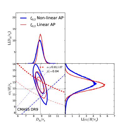
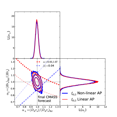
Throughout this analysis we apply the non-linear AP correction as described in Appendix A. In this section we investigate differences with the linear AP effect as used in Xu et al. (2012b). This linear approach was introduced in Padmanabhan & White (2008) in the formulation, and analyzed in in Kazin et al. (2012). However, as pointed out by Padmanabhan & White (2008), this linear approach breaks down when , which is clearly the case in the DR9-CMASS for a large part of the CL region.
The linear AP correction, when applied on the clustering multipoles, is as follows:
| (32) | |||||
| (33) | |||||
Here we neglect terms of order , as well as terms. (For a discussion of higher order terms see §2.2.4 in Kirkby et al. 2013.)
The left plot of Figure 13 shows the results obtained when applying the non-linear AP (thick blue) and the linear correction (thin red) as to the CMASS-DR9 . The dotted and dashed lines convey constant values of and , respectively.
The results clearly show that the linear correction under-estimates the uncertainties of and by and , where is the 68CLr of X=. The method results agree fairly well where is small (and regardless of ), but differ as grows. These differences should vary with the choice of the fiducial model, as well as the volume investigated.
We apply a similar comparison for a mock-mean signal (of 600 mocks) with the divided by three (as in §6.4) and plot the results in the right of Figure 13. In this higher S/N test we clearly see that the two methods agree with each other extremely well, due to the fact that is low. There is a slight under-estimation of the linear approximation at the CL region. Note that here we test the case where the fiducial and correspond to the mock true values (, ), whereas if we would apply a geometric distoriton of we should expect larger differences.
In conclusion, the non-linear AP correction should be applied to avoid potential estimation biases.
Appendix C Testing the algorithm on high S/N mocks
We test our methodology by applying it on a set of 100 mocks with higher S/N than those used in the final mock DR9 analysis. The motivation for this procedure is to separate between potential systematics and effects due to weak baryonic acoustic feature signals.
The higher S/N mocks, called “stacked-mocks", are built by stacking the 600 PTHalo DR9-volume mocks by groups of six, providing us with one hundred realizations. For purposes of this analysis we divide the DR9 (see §5.1.1) by a factor of six.
Figure 14 shows distributions of (-)/ and (-)/ for the stacked mocks (top) and the DR9 mocks (bottom) both pre- (left) and post-reconstruction (right). The quoted p-values are obtained when performing the standard Kolmogorov-Smirnov test between the distributions and a Gaussian one.
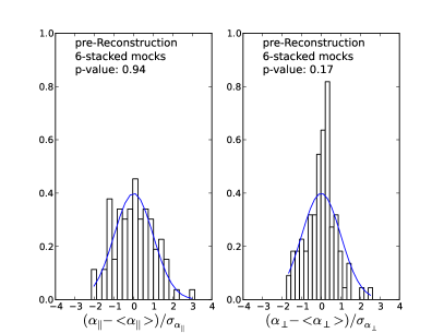
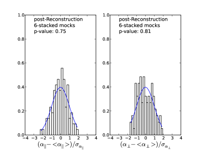
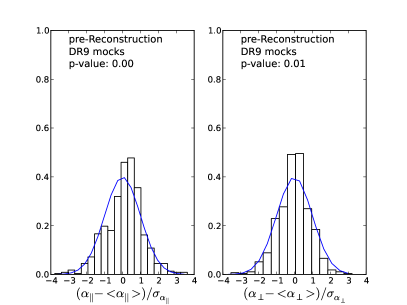
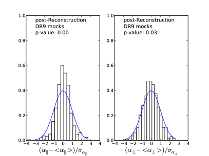
We find that the stacked mock results yield various Gaussian (or symmetric) attributes not found in the DR9 mock results. First, in the stacked mocks the means of the MCMC propositions are similar to the mode values, the standard deviations of the MCMC propositions are similar to the 68CLr and they yield low skewness values of the marginalized 1D likelihood distributions. As discussed in §6.2 in the DR9-volume mocks we find large skewness causing differences in these statistics. Using the DR9 mocks, we find in the that the modes and 68CLr are more reliable, as they are better defined.
One of the most important Gaussian-like features found in the stacked-mock , results is that the scatter in the modes is similar to the mean of the uncertainties. This is not the case for the DR9-volume mocks, probably due to weak anisotropic baryonic acoustic feature detections.
Finally, the stacked mock results (modes and uncertainties) are similar to those yielded when applying the same on the mock-mean signal (i.e., the mean signal of all 600 mocks). We find this to be true for all eight combinations investigated: clustering wedges, multipoles; RPT-based, dewiggled templates; pre-, post-reconstruction. All results are presented in Table 4.
| ( of realizations) | ||||
|---|---|---|---|---|
| RPT-based wedges pre-rec (100) | ||||
| RPT-based multipoles pre-rec (100) | ||||
| RPT-based wedges post-Rec (100) | ||||
| RPT-based multipoles post-rec (100) | ||||
| dewiggled wedges pre-rec (100) | ||||
| dewiggled multipoles pre-rec (100) | ||||
| dewiggled wedges post-rec (100) | ||||
| dewiggled multipoles post-rec (100) |
* The and columns show the median and rms of the modes.
* The and / columns show the median and rms of the fractional uncertainties.
C.1 RPT-based vs. dewiggled templates
As for preference of template (RPT-based vs. dewiggled) for constraining and , when using the stacked mocks we find strong cross correlation coefficients of in both modes and uncertainties. This comparison shows no difference in uncertainties. The only oddity we find is that the dewiggled pre-reconstruction wedges and multipoles yield median (mean) biases of () in modes, respectively, which is reduced post-reconstruction to (). These biases, when using the dewiggled model, do not appear when applied to the DR9-mocks. In those mocks, we find that the pre-reconstruction dewiggled model yields a bias of on determining .
In all four RPT-based cases (wedges, multipoles; pre-, post-reconstruction) the mean biases of are . Sánchez et al. (2008) thoroughly analyze differences between RPT-based and dewiggled and report that, when using the latter, one should expect systematic shifts in due to the lack of a -mode coupling term. In §5.2.2 we demonstrate that the post-reconstruction mocks do not prefer a template with , and hence suggest templates require a mode coupling term.
For all the reasons above our choice of preference is the RPT-based template.
C.2 Clustering wedges vs. multipoles
The stacked mocks show no significant difference regarding the constraining power of and on or ; post-reconstruction RPT-based yields sub differences. The cross correlation between the uncertainties of are found to be (dewiggled, RPT-based), and for . The pre-reconstruction templates yield similar results.
We then ask if multipoles and wedges yield similar mode results. The post-reconstruction stacked mocks indicate for and for in both RPT-based and dewiggled templates. Pre-reconstruction results yield similar correlations.
C.3 Improvement due to reconstruction
According to the stacked mock (and hence also ), we find the uncertainty of improves by and that for by .
The stacked mocks show that the modes should have a moderate correlation of and of . For a visual of results from the 3-stacked mocks, please refer to the top plot of Figure 12, which is described in §6.4.
Another value of interest is the cross-correlation between and . With the stacked mocks we find this correlation to be of order pre-reconstruction and post-reconstruction. Also we find no correlation between and modes, as expected.