![[Uncaptioned image]](/html/1303.4356/assets/x1.png)
DISSERTATION
Titel der Dissertation
Mutual information in interacting spin systems
Verfasser
Johannes Wilms
angestrebter akademischer Grad
Doktor der Naturwissenschaften (Dr. rer. nat.)
Abstract
This thesis combines ideas from the fields of quantum information and condensed matter. This combination has already proven extraordinarily successful: While one would naively assume that in condensed matter theory one would always have to work with an exponentially large Hilbert space, we are now beginning to understand that only a small part of these states is physically relevant. This understanding is primarily driven by insights about entanglement properties of the states actually occurring in nature; those insights have been delivered exactly by the application of quantum information theory.
In the spirit of these ideas, this thesis applies a quantity that is defined and justified by information theory – mutual information – to models of condensed matter systems. More precisely, we will study models which are made up out of ferromagnetically interacting spins. Quantum information theory often focuses on the ground state of such systems; we will however be interested in what happens at finite temperature.
Using mutual information, which can be seen as a generalization of entanglement entropy to the finite-temperature case, we can study the different phases occurring in these models, and in particular the phase transitions between those. We examine broadly two different classes of models: classical spins on two-dimensional lattices [1], and fully-connected models of quantum-mechanical spin-1/2 particles [2]. We find that in both cases the mutual information is able to characterize the different phases, ordered and unordered, and shows clear features at the phase transition between those.
In particular, in the case of classical spins on a lattice, we numerically find a divergence of the first derivative of the mutual information at the critical point, accompanied by a maximum within the high-temperature phase. We justify the location of the maximum by studying the behaviour of Fortuin-Kasteleyn clusters of aligned spins.
For fully-connected spins, we find a rather different behaviour: a mutual information that logarithmically diverges at the phase transition, as long as it is of second order; for a first-order phase transition there is no divergence at all. Analytical calculations in the classical limit support the numerical evidence. The behaviour is consistent with what one would have predicted from existing studies of entanglement entropy at the zero-temperature phase transition in these models.
Zusammenfassung
Diese Dissertation kombiniert Ideen aus den Bereichen Quanteninformation und Festkörperphysik. Diese Verbindung hat sich bereits als außerordentlich erfolgreich erwiesen: Es hat sich gezeigt, dass anstelle des gesamten, exponentiell großen, Hilbertraums nur ein kleiner Teil der Zustände tatsächlich physikalisch relevant ist. Durch Einsichten in die Verschränkungseigenschaften von Zuständen hat Quanteninformation hier wesentlich zu unserem Verständnis beigetragen.
In Anlehnung an solche Ideen wird in dieser Arbeit die Verwendung von mutual information (auch: Transinformation, gegenseitige Information, oder Synentropie) zur Beschreibung von Korrelationen in Festkörpersystemen motiviert und beschrieben. Dazu werden ferromagnetisch wechselwirkende Spinsysteme betrachtet. Im Bereich der Quanteninformation werden häufig die Grundzustände solcher Systeme diskutiert; in dieser Arbeit werden dagegen thermische Zustände bei endlicher Temperatur erörtert werden.
Mittels mutual information, die dabei als Verallgemeinerung von entanglement entropy (Verschränkungsentropie) für den Fall gemischter Zustände gesehen werden kann, können wir dann die verschiedenen Phasen dieser Modelle untersuchen, und insbesondere die Phasenüber-gänge zwischen ihnen. Wir werden im Wesentlichen zwei Klassen von Modellen betrachten: zum einen klassische Spins auf zweidimensionalen Gittern [1], und zum anderen vollständig verbundene Modelle quantenmechanischer Spin-1/2-Teilchen [2]. In beiden Fällen zeigt die mutual information charakteristisches Verhalten am Phasenübergang und innerhalb der geordneten beziehungsweise ungeordneten Phasen.
Insbesondere finden wir für klassische Spins auf einem Gitter mittels numerischer Me-thoden eine Divergenz der ersten Ableitung der mutual information am kritischen Punkt, verbunden mit einem Maximum innerhalb der paramagnetischen Phase. Wir motivieren die Existenz dieses Maximums durch Betrachtungen von Fortuin-Kasteleyn-Clustern von parallel ausgerichteten Spins.
Für die vollständig verbundenen Modelle zeigt sich ein anderes Verhalten: Die mutual information divergiert logarithmisch am Phasenübergang, sofern dieser ein Übergang zweiter Ordnung ist; für einen Übergang erster Ordnung gibt es keine Divergenz. Analytische Rechnungen im klassischen Grenzfall unterstützen hierbei die numerischen Ergebnisse. Das gefundene Verhalten ist konsistent mit bestehenden Resultaten, die bereits in anderen Arbeiten für die entanglement entropy des Grundzustandes gefunden wurden.
Chapter 1 Introduction and overview
The purpose of this thesis is to explore mutual information as a correlation measure, in the setting of a few selected spin models, at finite temperature.
In order to do this, I will try to generally motivate the study of mutual information, as a correlation measure, in chapter 2. This will mostly be based on an information-theoretic point of view. In particular, we will of course see the connection to entanglement entropy, to which mutual information sometimes reduces, and which was certainly a motivation for its study. I would however like to point out already at this point that this thesis is not concerned with a measure for “quantum entanglement”, which would allow to distinguish entanglement from “classical correlations”. It is well known that mutual information cannot provide that [3] – and while such a distinction is without any doubt very interesting, we will see that it might not actually be so relevant if one wants to use correlations to study phase transitions.
The bulk of the thesis will then be dealing with actually calculating mutual information in interesting model systems. They can all be understood as “spin systems”. There are essentially two very different classes that we will discuss: On the one hand, classical spins on fixed lattice positions, with local interactions, discussed in chapters 3 through 5. Some key results out of this group have been published as [1]. On the other hand, there are fully-connected spin models, where the spins all interact with each other rather than only with a small set of neighbours; this will be the subject of chapters 6 and 7. Again, some of the results have already been published, as [2]. The thesis finishes with some concluding remarks and an outlook.
Chapter 2 Mutual information
In this chapter I will try to generally motivate the study of mutual information in physical systems. The following chapters will then deal with its calculation for some specific systems, and also contain sometimes more specific motivation.
2.1 Motivation
I believe the most intuitive way to motivate the study of mutual information is the following: Take a look at figure 2.1(a). This tries to represent a rather generic physical system: some bigger system that is made up out of many smaller constituents. These constituents could for example be individual nucleons, or atoms, or molecules. Let us maybe call them just “particles” for now. They could be arranged in a regular lattice (such as in the figure, and also as discussed in the next few sections), or they might be more randomly distributed.
For the system to be interesting, the particles will have to have some interaction. This interaction makes them behave differently than if they were just isolated individual particles. In fact, there will now be correlations between the particles. For example, in a solid the individual particles are arranged in a regular lattice, which is obviously a very strong correlation between the particles.
As another example, closer to the systems that will be considered in this thesis, a ferromagnetic interaction means that particles (which you may in this case imagine as some sort of elementary magnets) will tend to all align in the same direction, which is clearly also some sort of correlation. But they will not always be perfectly aligned – there might be other factors that tend to counteract the perfect alignment, such as external magnetic fields, or temperature and entropy. In fact, at high enough temperature or fields, the ferromagnetic order typically vanishes, in a phase transition to an unordered (paramagnetic) phase.
It is therefore certainly important to try to actually quantify such correlations. Let’s stay with the example of a ferromagnetic interaction, and call the individual particles spins. A very well-established way to describe the correlations is the following: just consider two of these spins, as indicated in part (b) of figure 2.1. Maybe they could be described by classical values and . These could for example be allowed to be only and , representing orientation along some given axis. Maybe they would instead have to be described quantum-mechanically, in terms of spin operators, for which we could however just use the same symbols. In both cases, the concept of a correlation function is applicable: It is an expression like
that tells us how the expectation value of the product of the spin “operators” is different from just looking at the two spins individually. This is clearly an expression that tells us something about correlations between these two spins. It is called a correlation “function” because we can now study how this expression depends, for example, on interaction strength, temperature, external fields, or the distance of the two spins.
But don’t you find it a bit lacking? In particular, don’t you think it is rather arbitrary to pick out just two spins out of all of them? Certainly, in general there will be correlations in the system that we miss in this way, for which we would have to look at more than two spins at a time. Of course, this is well understood, and there are corresponding “higher order” correlation functions that involve more than two spins. But now, it is no longer so obvious which of these correlation functions we should refer to if we want to quantify the correlations, so is there maybe something else we could do?
Indeed there is: Imagine that you (virtually, not physically) divide the system into two parts, as indicated in figure 2.1(c). Then we would like to ask the following question: how much information can we gain about one part of it by looking only at the other one? It turns out that this is exactly what is known as mutual information!
So what is this mutual information? For a much more general (but also more abstract) discussion you can consult e.g. [4], but let me try to describe it in the setting I have started to lay out. The first thing we need to understand is that the state of a system at finite temperature is described by a probability distribution. This is also needed for the averaging in the correlation functions of course, but now we will make even more explicit use of the probabilities. In classical physics, in thermal equilibrium, the probability distribution is the well known Boltzmann-Gibbs distribution. In quantum physics, we will need a corresponding Boltzmann-Gibbs density operator instead.
The Shannon entropy [5] of a probability distribution
is a quantity that describes the uncertainty we have about the state of the system. If we now do our virtual bipartitioning, we write the index of a state instead of as with the understanding that and describe the state of the parts respectively.
This means we can now write the total entropy as
or
for the corresponding von Neumann entropy in the quantum case (see e.g. chapter 11 of [6] for more about the quantum case). It is of course clear that the classical case is just the special case of a diagonal density matrix; I still find it useful to write out the classical sums as well, as they make explicit the operations that are implicit in the quantum-mechanical trace.
Let us realize now that we can also find the probability distributions for the parts as the marginal probability distributions
In the quantum mechanical setting, we would have to take partial traces of the density matrix, “tracing out” the respective other part ([6], chapter 2),
We can now also calculate entropies of the marginal distributions, or reduced density matrices:
or
Now we are ready to define mutual information as
| (2.1) |
How can we understand that this is what we want? I very much like the following point of view: it is the uncertainty (“what we do not know”) about and “what we do not know about ” minus “what we do not know about the whole system”. Quite intuitively, this is the information that and have in common. Or, as described before, the information that we can extract from about and vice versa (note that the definition is symmetric).
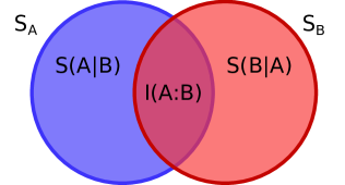
We can try to illustrate this with an “information diagram” as shown in figure 2.2 [4, 7]. The red circle represents , the blue one . The uncertainty about the whole system, , is the whole shaded area in the figure. If you subtract that from , you see that what remains is the “overlap” .
Also indicated in the figure is the relation to conditional entropies. As you can see there, we can also write the mutual information as
| (2.2) |
where is the entropy of given that we already know . You can easily see that this leads to the same interpretation of mutual information.
There is another important way to view mutual information: Let us write it out in terms of classical probabilities:
| (2.3) |
and you can see that this in fact a sort of “distance measure” between the actual joint probability distribution of the total system, and the product of the marginal distributions . It does not actually fulfill the axioms of a distance (you can immediately notice that it is not symmetric between and ). It is therefore labeled a “divergence” instead. More specifically: the Kullback-Leibler divergence of these two distributions (this is also called their relative entropy).
It seems intuitive to measure correlations by looking at how far the actual distribution is from a product distribution, so this is another nice interpretation of mutual information. It is also relevant for a different reason: The arguments I presented before rely on adding, or subtracting, entropies (or conditional entropies). This makes sense for Shannon/von Neumann type entropies, as explained for example in [4]. But these are not the only entropies out there, and such a property is not generally true for other definitions of entropy. If we wanted to work with Rényi entropies [8, 9] instead, the way towards a definition of mutual information should therefore certainly start from such a distance measure instead. More about this in section 2.5.
2.2 Mutual information and entanglement entropy
There is another strong motivation for mutual information that has already been mentioned in the introduction: It has been applied very successfully in a special case where it is usually known as “entanglement entropy”. You could also say that mutual information is a generalization of this by now pretty well-established concept. The special case is that the system is in a pure quantum state, which has therefore zero total entropy. A classical state with zero entropy is usually uninteresting, because the entropies of the parts will be zero as well. But pure quantum states can be strongly entangled, which reflects in nonzero entropies of the reduced density matrices. In that case, is called entanglement entropy. You will read more about mutual information as a generalization of entanglement entropy in particular in chapters 6 and 7.
2.3 The success story of mutual information
I would now like to argue that mutual information has proven a very useful concept in a huge number of applications, in many different branches of physics and other sciences. If you are already convinced of that, or do not care either way, feel free to skip this section.
In fact, I think the story of mutual information is such a success that it is impossible to even give an appropriate selection of references, not least because I am far from an expert in most of the applications. That is why I would like to point out only a very small number of references that I personally found particularly interesting: Mutual information seems to have turned out to be extremely useful for the alignment of (in particular medical) images: Imagine you have two different pictures of the same thing – say, one obtained by x-rays (computer tomography) and one obtained by magnetic resonance imaging, and you want to overlay them to get a better total picture (since they show different features differently well). The most effective way to get them to “match” seems indeed to be minimization of their mutual information, in a suitably defined sense, as originally described in [10, 11, 12, 13, 14].
Or, for an example that is maybe closer to your idea of physics, see [15] for an application in the context of dynamical systems.
All of these references are widely cited, but I found that many physicists are still pretty unfamiliar with the concept of mutual information and hence sometimes doubtful if it really can be that relevant. Therefore, I would like to go one step farther in trying to convince you that it has in fact proven useful. Indeed, let us try to quantify how much use it has found: First, let us look at articles submitted to arXiv.org, which is a preprint server with a strong focus on physics (and “neighbouring” sciences, such as mathematics or quantitative biology). We could even restrict to just papers that are explicitly categorized as physics, but the results turn out to be rather similar, so let us work with the largest possible data set.
Figure 2.3 shows the frequency of the phrase “mutual information” in the articles submitted to arXiv over a period from about 1995 (which is about the earliest date from which there is a reasonably good data basis) to the present. This graph is produced by arxiv.cultoromics.org; since we are not interested in any particular short-term trends or fashions, the data are smoothed by carrying out a rolling average over 12 months. It seems to be very clear to me that mutual information must have proven a useful tool – at least that is the only reasonable explanation I can offer for why it is now used more than five times as often that it was about 15 years ago. Of course that by itself would not be sufficient to argue that it is also relevant in the current context, but I certainly find this encouraging! I would like to point out that I only think this is a good indicator for relevance because the data spans many years – if it were just a short-term trend, you could easily argue that it is just currently “fashionable” and may well prove to have very limited use after all.
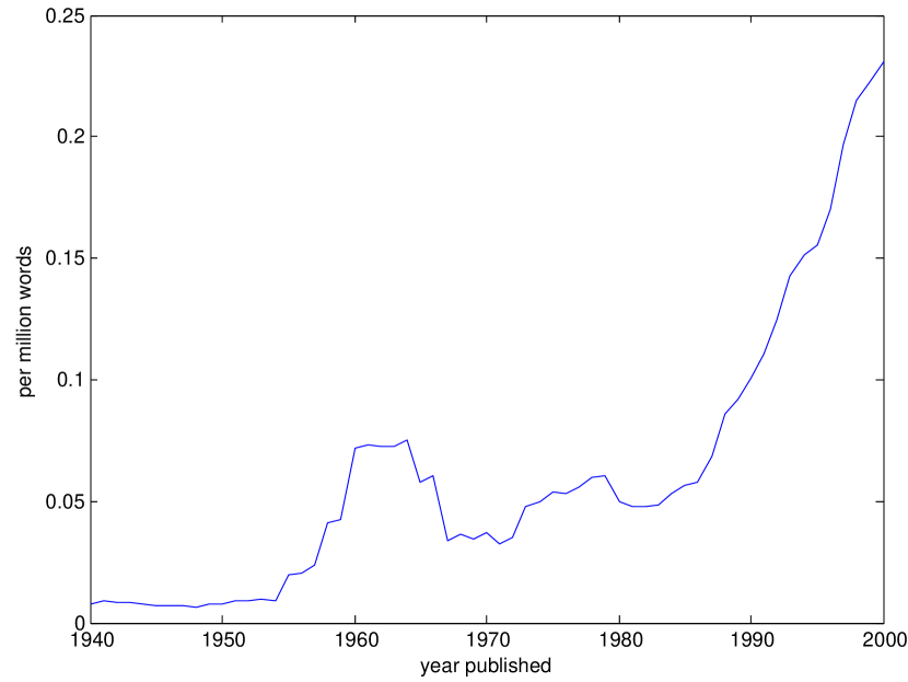
Since arXiv data only go back a relatively short period of time, I hope figure 2.4 can convince you that the success of mutual information is in fact a long-term one. The figure is based on [16] and the data available at books.google.com/ngrams (-gram is just a fancy term for a sequence of words; in this language, “mutual information” is called a 2-gram, or bigram). The figure is produced from the raw data “English, Version 20090715” which is considered the highest quality data set currently available. Of course, the frequency of the term “mutual information” in a general corpus of books is much lower than on the arXiv, but I believe we can again call it a pretty consistent success story. As an aside, you may try the phrase “information theory” at books.google.com/ngrams to convince yourself that it was indeed started by Shannon’s famous paper in 1948 [5].
2.4 What has been done?
Maybe you are now convinced that it should be a pretty obvious thing to try and look at mutual information. So, the next question is: has anyone else already done it? Judging by the title “Mutual Information in Ising Systems” of the paper [17] you would think it has been done at least in a setting similar to the one which will be discussed in chapter 4. However, that paper studies the mutual information of just two spins that are picked out, quite similarly to the study of correlation functions in fact. This is certainly also interesting (and turns out to be much simpler than what we are going to do), but cannot yield the new kind of information about many-body correlations we are looking for. You can also find a similar kind of study among the results of [18]. Yet another different definition of mutual information, as occurring between the steps of a Monte Carlo simulation of an Ising system, is presented in [19]. While very different from the approach presented here, it is also very interesting, and turns out to work well to determine the phase transition, something that we will also repeatedly be discussing (with our definition) in the following chapters.
Much closer to the spirit of this thesis are the works [20, 21, 22]. They present the same physically motivated idea of mutual information as a generalization of entanglement entropy. They study quantum spins on 2-dimensional lattices, which is not among the cases considered in this thesis, but it turns out that their results are not too dissimilar from what we will find for classical systems on these lattices, as will be shown in the following chapters. However, their (numerical) results are from my point of view severely limited by the fact that, in their Quantum Monte Carlo simulations, it is only possible to calculate Rényi entropies of reduced density matrices, with integer Rényi parameters larger than 1. They go on to use these to define mutual information according to (2.1). It does seem to produce useful results, but in principle the usage of this formula is not justified for Rényi entropies; as mentioned before, adding and subtracting entropies only really makes sense for Shannon/von Neumann entropies. Even just generally working with “raw” (non-smoothed) Rényi entropies can sometimes be very misleading. If you’re wondering now why all that is, or what Rényi entropies are at all, read on to the next section!
2.5 Generalizations
Of course there are some obvious generalizations to our definition of mutual information, the most obvious one being maybe dividing the system into more than just two parts. The aforementioned studies [17, 18] could indeed be considered an extreme limiting case, where the subsystems picked would just be single spins, with the rest of the system understood as a sort of background. If we wanted to study this more generally though, there will be a lot of freedom in our choice of the parts, and that is simply beyond the scope of this investigation. Also, in many cases the calculations will become infeasibly hard.
Another very interesting route would however be to study not just Shannon entropies (or their quantum generalization, von Neumann entropies). Possibly the most interesting other class of entropies are Rényi entropies [8, 9]
for a probability distribution , or in the quantum case
where is a “Rényi parameter”, and .
If you carefully take the limit for , you will see that you reproduce exactly the Shannon/von Neumann entropy (you will probably need l’Hôpital’s rule). This shows that this is obviously a possible generalization of the Shannon definition (because it reduces to that in this limit).
One advantage of Rényi entropies is that (integer) powers of density matrices may sometimes be calculated even where logarithms may not, such as was the case in [20, 21, 22].
Even more interesting is the fact that in some settings Rényi-type entropies may have a more concrete operational meaning. As outlined in [23, 24], Shannon entropy generally has an “asymptotic” interpretation: In the limit of a large number of realizations of a system, the uncertainty it describes can be made more tangible as both the amount of randomness that can be extracted from it and and its optimum encoding length (think of a compressed description of the system). If you have however just one realization of a system, these two things can be very different. If you want a measure of these quantities that is appropriate for a single realization of a system, you should look at Rényi entropies – maybe in particular the limiting cases and , also called max- and min-entropy respectively. Written out explicitly for a probability distribution , these are
and from this you may already see that they are related to compressibility on the one hand and amount of extractable randomness on the other hand. Max-entropy, which is simply the logarithm of the number of nonzero probabilities, is also known as Hartley entropy [25] and as such even precedes Shannon entropy.
In fact, it turns out that you might not even have to use these extreme cases, but that there are essentially two classes of Rényi entropies, namely the ones for and the ones for . However, all of this is only true if you apply “smoothing”, which means in calculating the entropy you optimize over all probability distributions within a certain distance of the one you are looking at. If you do not do this, Rényi entropies can become misleading and have very undesirable behaviour, because small changes in the probability distributions can lead to large changes in entropy. Maybe this is most easily seen in the definition of , which would be clearly changed a lot by adding very many very small probabilities (while slightly reducing a large one, for conservation of probability). Smoothing is the procedure to deal with such undesired behaviour.
This extra optimization step however (which is not required for Shannon/von Neumann entropies) makes those smoothed Rényi entropies much more complicated to deal with, at least numerically. Add to this the fact that for Rényi mutual information, we cannot start from (2.1) or (2.2), but need to find a good generalization of (2.3), and you see why this actually becomes significantly more involved than Shannon/von Neumann mutual information. And after all, the usual thermodynamic entropy is just Shannon/von Neumann entropy! Therefore, we will focus on the Shannon/von Neumann definitions from now on.
2.6 Phase transitions; area laws
As has already been hinted in the previous sections, we will generally be interested to study mutual information in the vicinity of phase transitions – we have argued that mutual information measures correlations, and phase transitions are where we expect the correlations to change strongly.
We will see that mutual information may even be used to “detect” phase transitions, meaning that by looking at the behaviour of mutual information you can conclude where (i.e., at what system parameters) the phase transition occurs. In the systems studied here, this is usually well known already, and can typically be found with less effort by looking at more traditional, “classical thermodynamical” quantities. In the systems studied here, you do not even need to bother with things like correlation functions, but straightforward “order parameters” will suffice. However, understanding the possible behaviours of mutual information is important anyway, because there are systems where traditional order parameters are not applicable and even correlation functions might fail. These are sometimes called novel or topological phases.
There is another aspect of mutual information that I should already mention in connection with phase transitions, which will be discussed in more detail within the following chapters: Remember the “classical thermodynamic” quantities such as correlation functions, or simply order parameters, with which we contrasted mutual information. In certain types of phase transitions, these show a very regular behaviour, independent of microscopic details of a system, but rather “universal” for a whole class of systems, which is then suitably called a universality class. The typical manifestation of such behaviour is in universal “critical exponents” that describe the functional behaviour of these quantities.
So is there anything similar for mutual information? There is indeed. Probably the most well known manifestation of such universal behaviour comes in the form of area laws [26]. They describe how mutual information scales with the size of the system, which is in many interesting cases not with the volume of the system, but rather its surface area – therefore the name area law. Area laws are something that has also been studied extensively in the context of entanglement entropy, see e.g. [27, 28, 29, 30, 31, 32, 33, 34]. We will see a clear instance of area laws in the following chapters!
While the correlations in classical systems will always strictly bounded by an exact area law [26], there may in general be corrections to the area law behaviour; and “universal exponents” might actually manifest in corrections, see also e.g. [35, 36].
In the systems studied in chapters 6 and 7, there is no notion of dimension (or you could say they are infinite-dimensional models). Hence, there is no such thing as area laws. Still, there are typical scaling behaviours that have been identified in the ground states of such models, e.g. in the entanglement entropy [37, 38, 39, 40]. In section 6.7 we will discuss similar behaviour that we found in the mutual information.
Chapter 3 Classical spin models on a lattice
In this chapter, we will consider how to calculate mutual information in a classical spin model on a lattice. The initial considerations will be independent of the lattice, but we will then specialize to two-dimensional lattices and in particular consider the case of a square lattice.
Key results of the calculations in this chapter and the next two have been published in [1], but a big part of the methods sections is previously unpublished, in particular the connection to matchgates as laid out in section 4.2.
Let us start from the definition of mutual information in the form of equation (2.3). This involves a sum over all the states of the system. Even for classical spins, these are exponentially many states: if we have spins that can take just two possible values, say , there are states. Clearly, carrying out such a sum quickly becomes intractable – even a pretty modestly sized lattice is out of reach.
One idea you might immediately have is to replace the exact sum by a Monte Carlo sampling [41, 42]. However, take another look at equation (2.3): what you then need to evaluate for each sample is a still pretty complicated expression involving marginal probabilities, which are not easily accessible – tracing out one subsystem involves an exponentially large sum again. Of course, you could argue that this could again be approximated using Monte Carlo methods. But if we had to do that in each step of the “outer” Monte Carlo run, it would be very inefficient – with Monte Carlo methods, you need to keep the updates simple, so that you can have the large number of samples you generally require for a good approximation.
However, such initial considerations are what finally lead to the following approach, which can in the end be used even without any involvement of Monte Carlo methods: You may notice that our formula bears some resemblance to a partition function, which is also a sum over all possible states of a system, although a simpler one:
| (3.1) |
In many cases, partition functions can actually be calculated pretty efficiently. However, our problem currently does not have the form of a partition function. But let us now also remember the result mentioned in section 2.6, that a classical spin system always has to fulfill an area law [26]. In a way, this implies that instead of summing over all the spins in the system, it should be sufficient to sum over just those that make up the “boundary” between the systems.
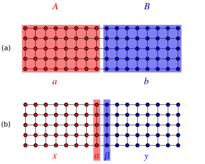
Let us try to combine these ideas into a way to rewrite the definition (2.3). We divide each subsystem into its “interior” and its “border” with the other system. The border is defined as the set of all those sites that share a bond with a site that belongs to the other subsystem; the rest makes up the interior. This is illustrated in figure 3.1: part (a) shows you the most straightforward way to divide a rectangular system into two parts and with states and . Part (b) shows how we identify the borders, for the states of which we will now use labels and , and the interior (or “bulk”) parts which we will label by and respectively. Therefore, we now divide the labels and for the states of the subsystems, as we used them in chapter 2, into and .
Now, we can rewrite the joint probability as where describes the contribution from bonds between spins all in the interior of , the contribution from the bonds between the interior and the border of , the one from bonds within the border, and so on. Plugging in this “factorization” of the probabilities, we find that we can rewrite the Shannon mutual information (2.3) as
| (3.2) |
Here the curly underbrackets identify “partial” partition functions, e.g. is the partition function of the system with the border fixed – we are summing over all sites in the interior of , but the border of has some fixed value.
We also have definitions of partition functions of “extended” systems. For example, means the partition function of the enlarged system , which has all of (both and in its interior, and is bounded by , which is the fixed border configuration for this partition function.
As you can see, the final sum is only over the spins in the boundary region, and . So, if we have an efficient way to calculate the partition functions in the formula – with given fixed boundary conditions – then we have reduced the sum over all the possible states to a sum over just the possible states of the borders.
In section 3.2, we will indeed see how partition functions can be efficiently approximated for arbitrary classical spin models in two dimensions. Chapter 4 will then deal with the classical Ising model, where there are even ways to calculate the partition function exactly, which we will also discuss in some detail there. Most of the results even for the Ising model will however be based on the approach of section 3.2, since it has some additional advantages. It is also the method used in chapter 5, which deals with some models that are not exactly solvable.
3.1 Monte Carlo sampling
What remains to decide – given a method to evaluate the partial partition functions – is how we carry out the remaining sum over the border states. For small enough systems we can certainly just carry out the sum exactly. For larger systems we will indeed use Monte Carlo sampling for this problem, which is now much more tractable than the original one. In particular, we no longer need to sample states of the whole system, but only of the border region consisting of and .
Let us spend a few words on why equation (3.2) is in fact in a form directly suitable for Monte Carlo: Monte Carlo sampling generally works for an expression of the form
| (3.3) |
where the form a probability distribution in the sense that they are real and nonnegative, and that we only get the value of up to the normalization of the , which we therefore need to have access to. Both of these conditions are fulfilled by the expression (3.2), where the obvious choice for the probability part is ).
What about the error we make by using Monte Carlo sampling rather than the exact sum? It is of statistical nature, and therefore proportional to where is the number of samples. It is also proportional to the standard deviation of the . But it also makes a big difference if we manage to have truly independent samples or if the samples are correlated. In fact, our samples will almost certainly be correlated; we will be working with what probably most people mean when they say Monte Carlo sampling, and that is Markov Chain Monte Carlo. Even more specifically, we will use the Metropolis algorithm, where, in essence, we start with a random sample, and new samples are proposed as updates of the current one, and accepted with a probability (or with probability 1 if is greater than ). In the next section we will see a way to calculate partition functions that allows for a particularly simple form of updates, i.e., updates that can be done very efficiently, with little computational effort.
There are a few more subtleties about the Monte Carlo algorithm, in particular the fact that you do not want to start with a completely randomly picked initial state, but only start the actual averaging after a certain amount of equilibration. Also, in order to estimate the error accurately for the case of correlated samples, it is not enough to just calculate the standard deviation of the samples, but one needs to take into account their correlation as well. We will follow the common approach and do it by a coarse-graining procedure: one combines neighbouring samples into bins and examines how the standard deviation increases as a function of the bin size. Once it is converged, one has found the effective standard deviation of uncorrelated samples, which one can use to estimate the error made in the Monte Carlo approximation.
3.2 Calculating partition functions
Now let us think about how to calculate partition functions for classical spin systems on a two-dimensional lattice. We follow ideas presented in [32, 26]. Let us assume the Hamiltonian has the form
where and are the (classical) spins and defines interacting sites, e.g. nearest neighbours. The partition function then is
| (3.4) |
with the “thermal” as opposed to the used to label boundary configurations. Let us rewrite the contribution of each bond as
where we introduced a new variable . In order for the above identity to be satisfied, needs to take at most as many different values as any of the classical spins involved. You can see that by taking e.g. a singular value decomposition of the left hand side (understood as a matrix with row and column indices and ). Then simply absorb the singular values into either or and you have exactly the desired form. This rewriting of a single bond is graphically illustrated in figure 3.2 (a) and (b).

We can now carry out the sums over the in (3.4), and let sums over the remain. Doing this, we create at each site a tensor which is constructed as the sum (over of direct products of s and s. The number of terms in the direct product (and therefore the order of the resulting tensor) is given by the number of bonds meeting at this site. This is illustrated in figure 3.2 (c) and (d).
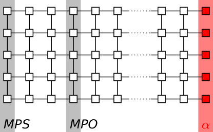
What remains to be done for the calculation of the partition function is the summation over the -indices, which corresponds to the contraction of the resulting tensor network. An example of such a network is shown in figure 3.3, corresponding to the evaluation of the partial partition function in the geometry discussed before. Fixing the state of the border can be understood as a specific choice of (unconnected) tensors on the boundary.
In this network, we can now understand each interior column as a transfer matrix which has a special form – it is a Matrix Product Operator (MPO) [43, 44]. For non-square lattices, you would need to be a bit more careful, but the principle remains applicable. The boundary (in figure 3.3, the leftmost column) can be understood as a Matrix Product State (MPS). The network can now be contracted by repeatedly applying MPOs to a MPS, resulting in another MPS to which we apply the next MPO, and so on. In principle, this is exactly the same as contracting the tensor network in any other way (although it is already much more efficient than if you were to write each transfer matrix in full form rather than as an MPO). The required dimension of the MPS does however grow exponentially.
The approximation will come from reducing the dimension of the MPS in this scheme. After we apply another MPO, we approximate the MPS by another one of lower bond dimension (typically chosen fixed in advance), thereby preventing the exponential growth. Of course, we lose information this way, and we will in fact examine the quality of the approximation in section 4.1.2.
One case is of particular importance, namely the case of a translationally invariant system (more precisely, it just needs to be translationally invariant along the horizontal direction in figure 3.3). In that case, all the MPOs are identical. We can now consider the case of a system that is very large in the horizontal direction. Now, what we do is repeatedly apply the same transfer matrix (given as an MPO) to a vector. It is clear that after many applications this vector will in fact be proportional to the eigenvector of the MPO that corresponds to its eigenvalue with largest magnitude (assuming that it is unique) [45, 46, 47, 48]. Now, there exist specific algorithms [49, 50, 43, 51] that can very efficiently determine an approximation for this eigenvector, in the form of an MPS with a given bond dimension. The algorithms can also make use of translational invariance in what is the vertical direction in figure 3.3.
Let us indeed assume the number of columns in the bulk is so large that we can make this approximation. We can label the largest eigenvalue , the corresponding eigenvector , and now the whole partial partition function discussed can be approximated as . Note how each application of the transfer matrix MPO contributes a factor of . What is really great about this formula, and remains true in an analogous way for the case of a network without translational symmetry, is that for a different border configuration we need only calculate the new overlap with rather than do the whole (much more complicated) tensor network contraction again!
It should be obvious that the other partial partition functions in equation (3.2) can be approximated in a similar way as . Let us now work with a rectangular system of columns total, in the limit , and divide it as in figure 3.1, exactly in the middle. If we assume periodic boundary conditions in vertical direction, this is actually a very long cylinder, cut in the middle. The partition functions are then , , , and . The partition function of the whole system, which is needed for normalization purposes, is Let us further introduce the shorthand . Let us also introduce unnormalized Boltzmann weights, where is the energy of configuration . Let us now work with these rather than the normalized probabilities . The can be factored exactly like the in the previous section, and we then get the following formula for the mutual information
| (3.5) |
which is independent of , so that the limit is unproblematic.
3.2.1 Simplifications
Can we simplify formula (3.5) even further? It would be a lot simpler if the logarithmic term were not there, because then we would just have
| (3.6) |
with the Ising transfer matrix, and because that can be written as a MPO, this expression would be easy to calculate as the contraction of a tensor network (and it is actually just the total partition function).
Of course we cannot simply drop the logarithmic term; but we can separate the logarithmic term into three parts, .
Now, is actually an exponential, of the sum over all the bonds between two columns: , where the sum goes over the rows and and are the components of the configurations and respectively.
The logarithm of the exponential is of course just the exponent , so we have to calculate
| (3.7) |
We can now consider the terms separately for each , and notice that they are all local and can therefore efficiently be calculated as a contraction with suitably modified MPOs.
What about the remaining parts, with and ? Let us look only at the one with ; the one with is exactly symmetric. We have
where we introduced a unit term in the logarithm and used that to separate it into two parts, one that has the form of an entropy,
| (3.8) |
and an additional term again containing the logarithm of an exponential, which becomes a sum of local terms that can be handled easily.
So what remains is just the term (3.8) that describes the entropy of the marginal distribution , normalized by . If we have the eigenvector , we can calculate this entropy: Just as discussed in section 3.1, for small numbers of rows the sum can be carried out exactly, and for large numbers of rows it can be approximated by Monte Carlo sampling.
In particular, note that for sampling the coefficients it is sufficient to know the eigenvector as a MPS, without ever needing it in exponentially large full form (the are straightforward to calculate anyway). As a consequence, we can do the sampling particularly efficiently by using Monte Carlo updates that sweep back and forth along the MPS and store intermediate contraction results. It might be worth noting that similar Monte Carlo sampling procedures for matrix product states have also been used in a rather different (variational) context [52, 53].
Chapter 4 The classical Ising model
In this chapter, we consider a particular instance of the classical spin models discussed in the previous one. The model under consideration is the famous Ising model [54] in two spatial dimensions. It has been solved exactly by Onsager [47]. In this case, that implies that there exist algorithms that allow an efficient evaluation of its partition function, in exact form rather than just as an approximated tensor network contraction. However, we will start by reviewing how the general tensor network approach specializes to the Ising model in section 4.1. In sections 4.2 and 4.3 we will then see two algorithms that make use of the special features of the Ising model. At the end of the chapter, we will discuss the results of the calculations, and see if they match our ideas about mutual information.
Let us start with the model definition: The classical Ising Hamiltonian is
| (4.1) |
where the spins have possible values or , and interactions are between nearest neighbours. We will generally consider the homogenous case , and restrict to the ferromagnetic . On bipartite lattices such as we will study, the antiferromagnetic case can directly be obtained by simply flipping all the spins of one of the sublattices.
4.1 Tensor network contraction
Let us go through the steps outlined in section 3.2 again, and see what they look like for the particular example of the Ising model.
4.1.1 Tensors
Introducing the shorthand notation , the partition function is
| (4.2) |
and we can rewrite the contribution of each bond as
| (4.3) |
where the new index only takes two values here, say and . Equation (4.3) can be satisfied by
and . Unsymmetric choices are also possible, where for example the -dependence is only in the s; it is even possible to completely take out the -dependence, and write
with
and
We can now carry out the sums over the in (4.2), and let the newly introduced sums over the remain. Doing this, we create at each site a tensor, which is constructed as the sum (over of direct products of s and s (or s and s). The number of terms in the direct product (and therefore the order of the resulting tensor) is given by the number of bonds meeting at this site. What remains to be done for the calculation of the partition function is the summation over the -indices, which corresponds to the contraction of the resulting tensor network.
Let us write down the tensors, using and . They have indices, say , , , and . We will later sometimes want to understand the tensor as a gate acting on two incoming indices, let these be and . The outgoing indices are then and . Putting the -dependencies in the outgoing indices only, we get
| (4.4) |
and you see that the s (that contain the -dependencies) can be completely separated from the s. We will pick up from that fact again in section 4.2.
4.1.2 Error analysis
Having found the form of the tensors, we can now follow the calculation outlined in section 3.2. The results for the Ising model will be presented at the end of this chapter. For now, let us only analyze the errors that come from approximating the largest eigenvalue and corresponding eigenvector by a MPS with limited bond dimension.
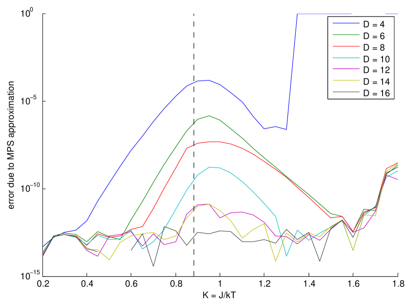
Since the focus of this work is not on Matrix Product States and their properties, let us only pick out one specific setting to discuss the general features. Figure 4.1 shows the error made by using a MPS of bond dimension rather than the exact eigenvector of the transfer matrix, for a system of 16 rows, where it is still possible to calculate that eigenvector exactly. To avoid any other error sources, it is of course necessary that we also carry out the summation of (3.5) exactly. This is indeed possible after the simplifications described in section 3.2.1.
We notice two things: First of all, the errors show a very systematic behaviour, and have a pronounced maximum (note the logarithmic scale). The maximum occurs where the system becomes critical, and this is exactly the behaviour we would expect from Matrix Product States.
Second, the quality of the MPS approximation depends strongly on the bond dimension. For the system studied, a MPS with bond dimension of is very close to the exact eigenvector, and for most temperatures the only difference is numerical noise. However, almost any choice of results in an error that will be lower than the statistical error we will introduce by Monte Carlo sampling. Since a smaller results in faster Monte Carlo updates, we will choose a relatively modest , in order to be able to do as many Monte Carlo steps as possible and minimize the total error.
Even if it will be the Monte Carlo sampling that decides our errors, let us dedicate the next two sections to methods for the exact calculation of Ising partition functions.
4.2 Matchgates
Let us remember the tensors (4.4) from the preceding section. We can rewrite them in matrix form, with being the column indices (corresponding to “incoming” indices) and being the row (“outgoing”) indices. We have with
We will now interpret these tensors/matrices as “gates” acting on some quantum state. The gates turn out to have a special form, they are matchgates [55]. As the name “gate” suggests, the context in which this has mostly been considered are quantum circuits, the gates in which are usually unitary. This also provides the connection to what has become known as fermionic linear optics [56, 57, 58, 59, 60, 61, 62]. We will work along similar lines, and map the tensors/matrices/gates to fermionic operators. However, the actual mapping is significantly different from what has been done in the literature – in particular, our operators are non-unitary.
4.2.1 Fermionic representation
So, let us now try to express the gates in terms of fermionic creation and annihilation operators. Without loss of generality, let us restrict ourselves to just two modes, which we can label and , with occupation numbers and . The state space is Fock space, states are given as
To determine the components, say or , we can project
| etc. |
Let us start by looking at the entangling gate . In terms of fermionic operators, this can be written as the operator in a transformed basis given by
Going back to the old basis, the bond-strength gates are just single-mode gates of the form
| (4.5) |
where is either of or A gate is required for each bond, i.e. at a typical site in the bulk there are two gates: one for the horizontal bond and one for the vertical bond.
The essential thing is that all of these gates are only quadratic in the fermionic operators. In the next section we will see how this allows us to efficiently describe the application of the gates using only a polynomially-sized covariance matrix, rather than a full exponentially-sized state vector.
How do we handle the boundary conditions needed for our partial partition functions? In the end there turns out to be a pretty simple way to handle them: what we do is fix the relative orientations of boundary spins by using infinite bond strengths. That is, if we want to implement a boundary configuration in which two neighbouring boundary spins are pointing in the same direction, we connect them by an infinitely strong ferromagnetic bond. Otherwise, we use an infinitely strong antiferromagnetic bond. This fixes the boundary configuration up to a possible inversion of all the spins at once. However, because of the inversion symmetry of the whole problem, both these configurations will result in identical values of the partition function. Therefore, we simply do the calculation with the spins only fixed among each other, and divide the result by a factor of two. The gates remain in fact well-defined even for infinitely strong couplings, if we renormalize them – since these infinitely strong bonds are not relevant for the partition function, this does not cause any problem.
If one prefers, one can even work without infinitely strong antiferromagnetic bonds at all: Rather than fixing the relative orientations of the boundary spins, we can achieve the same effect by fixing all boundary spins to point in the same direction, which only requires infinitely strong ferromagnetic couplings. We then simply invert the couplings that connect some of the boundary spins with the spins in the interior.
4.2.2 Calculating the partition function

Now, we know how to express the tensors as fermionic operators, but we still need to calculate the tensor network contraction to find the partition function. So how do we do that? We start from a state and begin applying the operators, and finally project onto again. However, why can this be done efficiently? Let us first see how we can identify modes such that the only thing that acts on them are the quadratic operators found in the previous section. Figure 4.2 shows how to do that in a square lattice by having the modes run at an angle of 45 degrees to the rows and columns of the lattice. The gates act on nearest neighbours and there is no problem in keeping track of signs due to fermionic anticommutation rules.
It is now really essential that the gates are only quadratic in the fermionic operators, because that means we do not need to work with a general fermionic state, but only with a fermionic Gaussian state. You can find more details about this class of states e.g. in reference [59]. In particular, what we will do is the following: Instead of working with an exponentially large state vector, we work only with its covariance matrix, which contains all the information if we apply at most quadratic operators. This covariance matrix can then be updated using Wick’s theorem [63], and we have all the pieces needed to calculate the partition function efficiently, i.e. with polynomial rather than exponential complexity. Let us see how these pieces indeed require only polynomial resources:
Covariance matrix
The covariance matrix contains the expectation values for all quadratic expressions of creation and annihilation operators of fermionic modes. We can order the operators for example as . A mapping to Majorana fermions [64] is also possible, but not necessary. The covariance matrix is then where is the expectation value with respect to the current state of the system. Applying a gate operator means transforming into , or transforming the expectation value as .
Wick’s Theorem
So, what we have to do is update the covariance matrix by applying some fermionic operators, thereby inducing a transformation of the covariance matrix. To calculate the transformed expectation values in the covariance matrix, we can use Wick’s theorem
i.e. what you have to calculate is the Pfaffian of the matrix restricted to rows and columns . In particular for the case of just 4 fermionic operators (which turns out to be all that is actually needed)
What is that Pfaffian in general? We will give a proper definition and discuss it in more detail in section 4.3.2. This is already a hint that the method presented in the next section does in fact make use of the same intrinsic properties of the Ising model, even though the actual manifestation will look pretty different.
4.3 The FKT method
In this section, we will revisit a long-established method used to calculate Ising partition functions, which can be formulated without any understanding of the (partial) partition functions as tensor network contractions. While the method itself is old, we will see that it can also be adapted to deal with the fixed boundary conditions needed for our partial partition functions. Maybe even more importantly, we will also see how it can be used in such a way that changing of the boundary conditions requires only a small amount of new computation, just like with the MPS method discussed in the previous chapter.
4.3.1 Ising partition function as a dimer covering
So how does this method calculate the partition functions? Let us start by following the treatment of chapter V of [65]. For simplicity of exposition, let us work in the homogenous case, but it should be obvious that the following can straightforwardly be generalized to interactions of varying strengths, just as in all the other methods we have discussed. As , and consequently also can only take on the values and it holds that and consequently we can write the partition function as
where is the number of bonds in the lattice. Expanding the product gives us (exponentially) many terms, which have some factors of and some factors of the type , and in fact any can turn up at most in a power equal to the coordination number of the lattice, so for a quadratic lattice up to . More interesting though is that terms that have an odd number of any will vanish once the sum over this is carried out. The only remaining terms are those that contain even powers of every appearing in them, and those will pick up a factor of from each sum over some so a total factor of , where is the number of sites in our lattice.
We want to represent every such term by “marking” the bonds appearing in it in the lattice. The condition that we can only have an even power of means we have a configuration where at each site an even number of marked bonds meet. This leads to a configuration consisting of one or more closed loops of connecting bonds, and we get the product of as many as there are bonds in the loop(s). The loops may intersect but cannot share segments. In the literature you will sometimes also read that these allowed configurations are called polygon configurations (if you draw the graph using straight edges, closed loops are polygons).
So all in all we have
where we sum over all configurations fulfilling the above conditions, with the suitable weight given as the product over the weight of all the bonds in the configuration. You can indeed notice that the above formula can be generalized to lattices where each bond has, in general, a different strength :
| (4.6) |
What we now want to do is calculate this weighted sum over closed loop configurations. Let us now follow the presentation of [66], but with updated terminology. We will map each loop configuration to a “perfect matching”, i.e. a set of edges such that each vertex is part of exactly one edge in the set. This sort of matching is exactly what gave the name to the matchgates that were mentioned in the previous section.
The mapping to perfect matchings can be achieved by extending the lattice; let us illustrate it for a lattice where each vertex has a coordination number of four, i.e. the square lattice. The nicest way is to replace each vertex by six new ones and map the possibilities of an even number of bonds meeting there, of which there are
to the eight possible perfect matchings as shown in figure 4.3. In order not to change the weight of each contribution in the partition function, it is necessary that all the extra bonds introduced must have a weight of unity.

4.3.2 Dimer covering calculated as a Pfaffian
Using this construction, we can build up the extended lattice, as is shown in figure 4.4. Now, the essential ingredient is what is sometimes called the FKT theorem after Fisher, Kasteleyn, and Temperley [67, 68, 69]. It tells us that we can calculate the partition function, i.e. the sum over all the weighted dimer coverings, or perfect matchings, as the Pfaffian of a suitably constructed matrix. Crucially however, it must be possible to orient the edges of the lattice graph in a specific way, such that every possible loop contains an odd number of bonds oriented in clockwise direction, as indicated by the arrows in figure 4.4. Such an orientation can always be found for planar lattices, but in general not for arbitrary lattices. This is what ultimately restricts this method in the same way that the mapping to free fermions and matchgates is restricted. Let us now take a closer look at this Pfaffian, which also occurred in section 4.2.2.

What is a Pfaffian?
The Pfaffian of a antisymmetric matrix is conventionally defined as
| (4.7) |
where the sum is over all possible permutations of It can however also be written as a sum over all partitions of into pairs . Let us call the set of all such partitions . We then get
| (4.8) |
where is the same as ) for one of the corresponding permutations , one of which would be
| 1 | 2 | 3 | 4 | ||||
|---|---|---|---|---|---|---|---|
.
There are ways to order the pairs, and two possibilities to order each of the pairs, so that the factor in the definition (4.7) is exactly canceled, and we might really say (4.8) is the more natural definition. It is pretty obvious that equation (4.8) provides the required connection to the weighted perfect matchings, which are exactly such partitions into pairs. Note that it is crucial that we can assign the correct signs, which means this only works if it is possible to find a suitable orientation of the lattice.
Relation to determinant
We realize that the matrix of which we need to calculate the Pfaffian is essentially just a weighted oriented adjacency matrix, and its dimension is therefore just the number of sites. But the definitions of the Pfaffian still seem to involve exponentially many terms, so how can it be calculated efficiently? For this, we can use the identity , for we know efficient methods to evaluate determinants. Efficient means in time polynomial rather than exponential in the size of the matrix. To be precise, (4.8) consists of terms, just as the usual definition of a determinant of a () matrix does:
but this can nevertheless be computed in time , e.g. by doing a LU decomposition (see below).
Efficient evaluation of the determinant
So the evaluation of a determinant is already efficient, but for the final calculation of the mutual information we actually have to repeatedly calculate determinants of still pretty big matrices where only very few entries (those related to the boundary conditions) change, while the “bulk” remains unchanged. In this situation, we can do better still, as the determinant of a matrix can be split into factors
| (4.15) | ||||
| (4.16) |
so if just the block, assumed to be relatively small, changes, we just have to calculate the determinant of the big block once, and find once the (again relatively small) matrix , and each time we want the determinant of the changed full matrix we can then get away with calculating a determinant of a matrix of only this small size.
Numerical computations of the determinants
Since the calculation of determinants is the essential computational step, let us spend a moment discussing it: The standard way to calculate a determinant numerically, is to do a LU decomposition of the matrix in question. This decomposes a matrix into a product of two matrices and , , such that is a lower triangular matrix and is an upper triangular one. The determinant of a triangular matrix is simply the product of its diagonal entries, so the determinants of and can be easily computed, and the determinant of is then given as due to the multiplicativity property of the determinant. In fact, a typical LU decomposition even produces an with unit diagonal, such that and therefore , and we just need to multiply the diagonal elements of .
Especially for the full matrix (but also for the reduced ones, depending on their size) the determinant is a very big number. This is not so surprising: If all the elements on the diagonal of are greater than 1, the number will grow exponentially with the matrix size. If they are all smaller than 1, the determinant will become exponentially small. While these conditions may not occur often with more general matrices, they are pretty typical for the ones we have to deal with, and neither exponentially small nor exponentially large numbers can be handled particularly well in the usual floating point representation [70] – you can lose precision, or, in the worst case, numbers can even become too large or small to be represented at all (overflow or underflow). However, we can work perfectly well with the logarithms of these numbers, and therefore we can simply use a custom routine for the determinant calculation that does just that.
Bond strengths and boundary conditions
As mentioned at the beginning of this section, one other thing that goes beyond the established FKT algorithm is the handling of the fixed boundary conditions. In fact, it turns out to be pretty straightforward once you realize that we you again employ the procedure described at the end of 4.2.1, and use bonds of infinite strength to fix the boundary in itself (and take care of the extra factor of two introduced). It turns out that we can again avoid any possible problems with infinities, because only the hyperbolic tangens of the bond strength is relevant, and that is simply for an infinite bond strength. Seemingly divergent terms like the -terms in (4.6) will always cancel for the relevant partition functions.
4.4 Results
The preceding sections contain all the information needed to successfully implement the calculations algorithmically, e.g. as Matlab programs. It is a bit of a challenge to get all the different normalization factors correct, but in the end of course all the algorithms give the same results, so that there is little to show or discuss here, and we can simply use whatever algorithm seems most appropriate for a given problem geometry.
In particular, we want to work with systems that are as large as possible and therefore require Monte Carlo sampling. For the geometry introduced in figure 3.1 the MPS approximation method turns out to be most convenient in practical implementation, and as we have seen in section 4.1.2, the error is typically limited by the statistical Monte Carlo error rather than the approximation of the eigenvector.
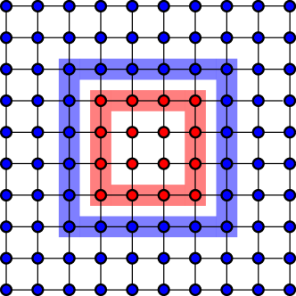
One geometry is however a bit limited, so is there a second choice of geometry that would be interesting? In fact, there might be an even more natural one: Not just one system that is cut in the middle, but one system that it is fully embedded in a bigger one. This is illustrated in figure 4.5. For such a geometry the MPS method is less convenient, which is why the results presented are obtained by the FKT method (with Monte Carlo sampling of the boundary configurations again). The matchgate method is of course also suitable, but its Matlab implementation turned out to be somewhat slower in practice.
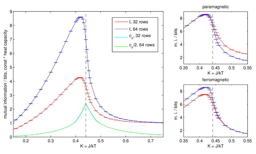
So let us take a look at the results, shown in figures 4.6 and 4.7 for the two respective geometries: Figure 4.6 shows the results for the geometry introduced in figure 3.1, of a strip that is cut in the middle. The strip is assumed to be infinitely long in horizontal direction, which is another advantage of the MPS method, avoiding any finite-size effects in that direction. Also, we can most easily employ periodic boundary conditions in the vertical direction, which makes for a much larger effective system than open boundary conditions, and means that we are working with a cylinder rather than a strip. This is in fact also possible with for example the FKT method, but increases the number of Pfaffians that have to be calculated there.
Let us start by taking a look at the general features of mutual information: We notice that it goes to zero for high temperatures. That is exactly what we would have expected: at high temperatures the spins are all randomly aligned, and if you look at the spins in one of the subsystems, this does not give you any information about those in the other subsystem.
At low temperatures, the mutual information, calculated using a base-2 logarithm, becomes 1, i.e. 1 bit. Again, this is exactly what should happen: All the spins will be aligned either up or down. In any case, looking at one part of the system tells us that the spins will be aligned in the same way in the other part, which is exactly 1 bit of information.
In between those two limits, there is a phase transition. Its location in the thermodynamic limit is known exactly, and indicated by the dashed black line at . Clearly something is happening around there, again as we would have hoped. However, the naive reasoning may have gone like this: We know that at criticality the correlation length, which describes the spatial behaviour of the correlation function, diverges. That is why maybe the most natural thing would have been to expect a maximum of the mutual information exactly at the critical point. However, the maximum lies within the high-temperature (paramagnetic) phase. Still, there is something happening at the phase transition: It appears to be an inflection point of the curve and the point of the largest (negative) slope. In fact this slope, i.e. the first derivative of the mutual information, will obviously diverge in the thermodynamic limit. You can see that for example by comparing the results for two different numbers of rows (circumferences of the cylinder) that are shown in the figure.
To be specific, results are shown for both 32 and 64 rows. Let us however first take a look at the heat capacity, which can be straightforwardly calculated as a suitable second derivative of the logarithm of the full partition function
It has been scaled by some arbitrary factors to be nicely visible in the figure and is plotted in cyan and green, respectively. You can see that it has a sharp peak near the location of the phase transition in the thermodynamic limit. This is already a first indicator that our system sizes are sufficiently large to make useful statements.
Let us however focus on the plots of the mutual information now. It turns out that it shows a remarkably simple scaling behaviour with the system size, scaling linearly with it in the paramagnetic regime. In the ferromagnetic regime, you first need to subtract 1, the value of the mutual information in the low-temperature limit, and then you recover exactly the same linear scaling. This can be seen in the right parts of figure 4.6, where the data for 32 rows have been scaled as described and are contrasted with the data for 64 rows. You can see that these scalings indeed work very well; there appear to be very little residual finite size effects. Also, you notice that not both of the scalings can work at the phase transition – unless this is indeed a point at which the slope becomes infinite in the thermodynamic limit.
The error bars might deserve an additional explanation: They show the Monte Carlo errors, calculated by a binning procedure as described at the end of section 3.1. The bond dimension of the MPS was chosen , such that the errors due to this approximation are lower than the ones introduced by Monte Carlo sampling even at the critical point.
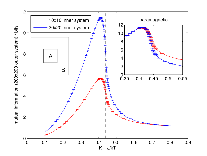
Let us now take a look at the second geometry, where the two parts of the system are nested within each other. The results are shown in figure 4.7, and are now obtained by using the FKT method as described in section 4.3. We find pretty much the same behaviour as in the cylindrical geometry, which serves as a nice confirmation of our results. In particular, we even find the same scaling in the paramagnetic phase. This is shown in the inset of the figure, where again the data for 32 rows has simply been scaled by a factor of 2. The ferromagnetic phase appears to be a bit more complicated in this geometry, and does not exhibit a straightforward scaling behaviour any more. Again the error bars show the Monte Carlo errors; remember that the FKT method itself is numerically exact.
4.5 Fortuin-Kasteleyn clusters
Can we understand why the mutual information has a maximum not at the phase transition, but within the high-temperature phase?
What follows is certainly not a full explanation, but a motivation which you may or may not find convincing: For spin systems like the Ising model, it is sometimes useful to consider clusters of aligned spins. For example, single spin updates can become very inefficient in Monte Carlo sampling methods, when the typical cluster size diverges at the critical point. What one therefore does instead is work with Fortuin-Kasteleyn (FK) clusters [71]. Those are clusters of spins pointing in the same direction, but not the simple geometric clusters that would arise from combining all neighbouring aligned spins. Instead, we only connect spins that are pointing in the same direction with a probability where is the energy difference between two aligned and unaligned spins, and the inverse temperature. This procedure results in clusters which can be treated independently from each other, which then allows for efficient Monte Carlo updates that flip the whole clusters. If one did not use this procedure, but always connected aligned spins, you would form clusters even at infinitely high temperature (), simply because neighbouring spins will sometimes happen to randomly point in the same direction.
So how can we make any argument about the behaviour of mutual information by looking at clusters? It is true that spins within a cluster are always perfectly correlated. So whenever a cluster lies in both parts between which we calculate the mutual information, it represents some information that is accessible in one system about the other one. It is not obvious how one would exactly quantify that amount of information, since we do not know how far any given cluster will extend into the other part; but we can nevertheless think of some interesting quantities: Namely, we can implement a Monte Carlo simulation that identifies FK clusters, using for example the Swendsen-Wang algorithm [72]. We can then ask how many of these clusters lie in both parts of the system; in other words, how many clusters would be cut if we were to cut the system in half. We can also ask for a slightly different thing, namely, in how many pieces each of this clusters would disintegrate. Since it might turn into more than two pieces, this is a slightly different measure.
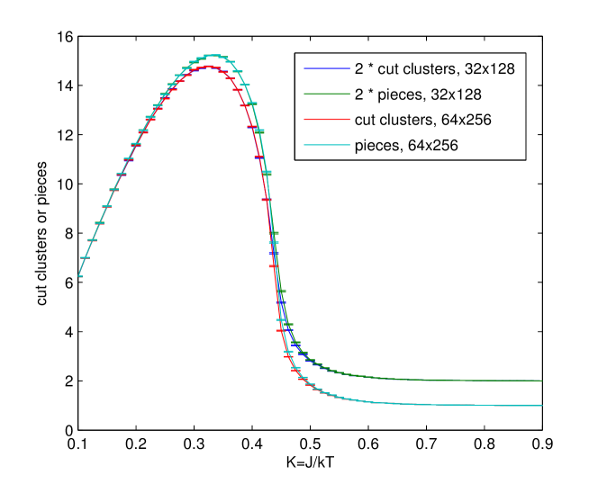
Take a look at figure 4.8 for the results. We again looked at the same cylindrical geometry as for the results in figure 4.6, so as to allow for greatest comparability. Instead of a cylinder that is infinitely long in horizontal direction, we just used a very elongated one, such that all relevant clusters were contained within it. Again, let us look at the cases of 32 and 64 rows circumference. You see that we recover many of the behaviours of mutual information: At very high temperature, there are no clusters to be cut. At low temperature, there is just one big cluster. In particular, also the scaling behaviour is exactly the same as for the mutual information: For high temperature, we find a perfectly linear scaling, no matter which of the two slightly different quantities “clusters cut” or “resulting cluster pieces” we study. For low temperature, we again need to take the “residual” contribution of the one big cluster into account.
We also see that these quantities show the same behaviour as the mutual information near the phase transition: There is again an inflection point at the critical temperature, with diverging slope. And again we have a maximum in the paramagnetic phase, and now we can give an interpretation of this maximum in terms of clusters: The phase transition may be the point where the cluster size diverges, but if our measure is instead how many clusters we can cut (or into how many pieces we can cut them), it is clear that the maximum of such a quantity will not be at the phase transition, but at higher temperature, where there are more clusters that can be cut – but also not at very high temperature, because there the clusters become too small, until they just consist of individual spins.
So, if we accept that the “cut clusters” quantities capture some of the essential properties of mutual information, I believe we have found a good intuition for why it behaves the way it does.
4.6 Related studies in the Ising model
At this point, some other studies made in the Ising model deserve mentioning [35, 36]. They study entropies of the probability distributions of boundary configurations in the 2-dimensional Ising model in a cylindrical geometry. This definition of entropy is actually very similar to the term (3.8), which appears as an important part in our calculations of the mutual information, and they are able to establish very nice scaling properties and relations to conformal field theories. However, there does not seem to be a way to actually connect this with our results concerning the mutual information.
Chapter 5 More lattice spin models
In this chapter, we will take a look at a few models which may be understood as generalizations of the Ising model. The essential generalization is that the spins can now take more than two different values; you might imagine it for example as a spin which can point in more different directions than just up or down. Two different generalizations of the Hamiltonian then lead to either the Potts models or the clock models.
5.1 Potts models
Let us start with the Potts models [75, 76, 77], defined by the Hamiltonian
If the only take two different values, this is indeed identical to the Ising model (4.1), up to a scaling of the coupling constant by factor of two (and an irrelevant constant energy shift). Now however we will let them take different values. The critical temperatures for Potts models are known exactly, just like for the Ising model. They are [77].
While we no longer have methods for exact solutions, like they were available in the Ising model, we can still numerically calculate the mutual information using the method explained in section 3.2. Figure 5.1 shows the results for rows, up to . It should be noted that for larger , the calculations become harder: We need to work with MPOs and MPSs with larger bond dimensions, and there is a bigger space of boundary states that needs to be sampled.
So what do we see? In short, pretty much the same behaviour as in the Ising model: A maximum in the high-temperature phase near the critical point, which again seems to be an inflection point with diverging slope. The maximum becomes larger with larger , which also makes sense of course – there can indeed now be a bigger amount of correlation, or shared information if you will. It is known that for the phase transition should change from a second-order phase transition to a first-order one. However, there is nothing notably changing in our results.
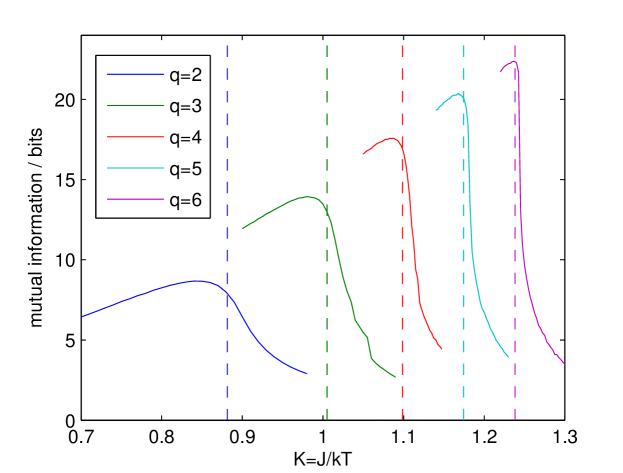
5.2 Clock models
The previous section described what is now known as the standard Potts models. These are however not the only possible generalizations of the Ising model. In fact, even Potts himself originally studied something a bit different, which is now usually called planar Potts model, vector Potts model, or clock model. Let us stick to that last name for clarity. Again, we have possible states for each site/spin, and let us now explicitly understand them as (planar) angles where . The Hamiltonian of the -state clock model can then be defined as
For , the clock models are different from, and rather more complex than the Potts models; and not much seems to be known about their phase transitions. Therefore, let us first take a look at the heat capacity, which we can also easily extract from our calculation of partition functions, just as we did before, for figure 4.6. The heat capacities behave pretty much like has been found in [78, 79, 80]. Figure 5.2 shows our results for the heat capacities for . For , the heat capacity has a pronounced maximum that is a good match for the location of the phase transition, which is known exactly in this special case [81, 82] and indicated as the vertical dashed blue line. For however, the clock model apparently has not just one, but two phase transitions. There are in fact also two maxima of the heat capacity, but these are not very sharp. They also do not match very well the estimated locations of the phase transitions; the dotted red lines show the estimates of [80] for .
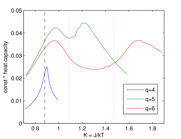
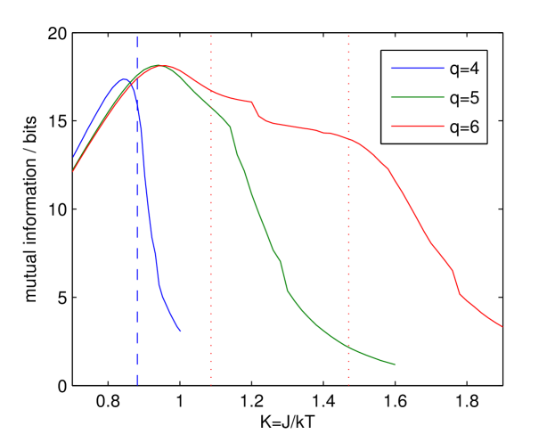
Correspondingly, we also find a rather straightforward behaviour for the mutual information in the case, see figure 5.3 – it seems essentially the same again as for Ising and standard Potts models, with a maximum near and the inflection point at the phase transition. This is actually not so surprising because this case can be related to regular Ising models [81, 82].
For and 6, the models clearly become more complicated. Since the different phases in the models are not very well understood, it does not seem possible to say much about the behaviour of the mutual information either. Again, there appear to be inflection points close to the suspected locations of the phase transitions. They now seem to be accompanied by some sort of slight “kinks”.
5.3 Quantum spin models
As has already been mentioned in section 2.4, there have been some independent investigations in quantum spin models [20, 21, 22]. These works made use of so-called replica tricks to allow for calculation of integer Rényi entropies in an adapted Quantum Monte Carlo simulation. As far as the results can be compared, they find some similar features as we did: a maximum within the high-temperature phase, an inflection point at criticality. However, their results are critically limited by the fact that they have to calculate mutual information according to (2.1) while using Rényi entropies, which is not well-justified from an information-theoretic perspective; there is also no smoothing, which is generally necessary to give a clear meaning to Rényi entropies, as was discussed briefly in section 2.5. Therefore I will not try to make any further connections between the results.
Chapter 6 The Lipkin-Meshkov-Glick model
In this chapter we will start to consider a very different kind of model. It can also be understood as a model of interacting spins. But rather than having only local interactions as in the previous chapters, these spins will now all be interacting with each other. Such a model is therefore also called a fully-connected model (the graph which describes the interactions as edges between the nodes representing the spins is fully connected) or sometimes also a collective model.
The model studied in this chapter is the Lipkin-Meshkov-Glock model, which can be seen as the fully-connected version of an Ising-type model and which has received the most attention of all fully-connected models; a subset of the results of this chapter has already been published as [2]. The chapter after this one will then deal with some more general fully-connected models.
6.1 Motivation
Most readers will probably agree that the assumption of having local interactions is a very natural one, and might therefore doubt if it even makes sense to consider fully-connected models. So where does the Lipkin-Meshkov-Glick (LMG) model come from, and is it even relevant for anything other than maybe a very small system?
The model got its name when it was studied by Lipkin, Meshkov, and Glick in the 1960s [83, 84, 85]. Stigler’s law of eponymy [86] applies, meaning it may be named after them, buy they are not its original discoverers: As they mention themselves in their first paper, it had certainly been discussed before that, e.g. in the (otherwise unpublished) PhD thesis of Stavros Fallieros [87].
Even though Lipkin, Meshkov, and Glick were working in the field of nuclear physics, and thinking about the spin-1/2 particles of neutrons and protons, they did not think about a model with spin-spin interactions in the same sense as e.g. in the Ising model, with a “magnetic” (ferromagnetic or antiferromagnetic) interaction between spins. Indeed, in a nucleus that is not a very relevant interaction – the relevant interaction is instead the strong nuclear interaction. However, in order to arrive at the LMG model the exact form of the interaction is not actually relevant. What is relevant is the fact that one has a system of fermions that arrange themselves in shells; the analogy to spin-1/2 systems comes about via fermions that can be in either of two possible shells, thereby forming effective two-level systems. Assuming some natural symmetries then leads to the LMG Hamiltonian.
Since the precise form of the interaction is not important in arriving at the LMG Hamiltonian, it turns out to work as a simple model Hamiltonian in quite a number of other systems as well. Typically, these are systems of fermions that form shells, like the nucleons in a nucleus do, but the interaction itself can be very different [88]. A prime example of such systems are metal clusters, but the same is also true for droplets of helium-3. There are also connections to, for example, Bose-Einstein condensates [89], or circuit quantum electrodynamics [90].
Another strong motivation to pick the LMG model for further study is the fact that in recent years, its ground state entanglement properties have received a lot of attention [91, 92, 93, 94, 37, 38, 39, 40]. We can therefore hope to be able to study how these relate to what we will find at finite temperature. In particular, the model has a phase transition both at zero and at finite temperature. In section 6.7 we will see how in fact the mutual information shows a comparable scaling behaviour to the ground state entanglement entropy, in the form of a logarithmic divergence in both cases.
6.2 Hamiltonian and symmetries
We will use the LMG Hamiltonian in the following form:
| (6.1) |
which shows very clearly how it can be understood as a system of two-level systems – spin-1/2 particles, if you like. In this language, every spin interacts with every other one. Let it be noted that this is not quite the most general form, but the form in which it has generally been studied recently. In particular, note that there is a ferromagnetic coupling between spins. In the next few sections we will deal, for simplicity of exposition and readability, with the special case of , and only afterwards go on to consider the effects of a nonzero .
The essential property of this Hamiltonian is that all the interactions are exactly identical, which is a symmetry that makes this system much more accessible than a general system of spins. One can see this by introducing the total spin , component-wise:
and then one sees that this symmetry implies that the Hamiltonian commutes with the magnitude of the total spin, . We can in fact rewrite the Hamiltonian, up to constants, as
The symmetry implies the following: If you think of the Hamiltonian of spins-1/2 as a matrix, this matrix can be brought into block-diagonal form, where the blocks correspond to different representations of the total spin, indexed by the magnitude of the total spin.
Why is this such a useful property? The reason is that this hugely reduces the complexity of numerically approaching the problem, because we no longer need to handle a Hamiltonian that is exponentially large in the number of spins. Instead we only need to deal with blocks of the size of the angular momentum representations. The possible values of total spin lie between or and . If is even, only integer values of appear; otherwise, only half-integer ones. The size of such a representation is , and there are only different possible values of . The exponential size of the full Hamiltonian is reproduced by the multiplicity with which these representations appear, but these are just numbers that can be calculated rather easily and of course be handled much more efficiently.
It will turn out that calculating mutual information is still far from easy, but let us get a little more familiar with the model first.
6.3 Phase diagram
Rather than just the one parameter of e.g. the classical Ising model on a lattice we now have several independent parameters. Therefore it seems appropriate to spend some time to get familiar with the phase space of the model, in particular since I am not aware of any suitable existing review. It will be convenient to set (i.e., expressing temperature in units of ), and sometimes to work with the inverse temperature .
6.3.1 Mean-field theory
Let us continue to interpret the model as interacting spin-1/2 particles and stick, for now, with the case of the Hamiltonian (6.1), i.e.
We have a ferromagnetic interaction, and if we just apply our intuition from spin models on a lattice, we suspect (correctly) that there will again be an ordered (ferromagnetic) phase and a disordered (paramagnetic) phase. In fact, the average magnetization in -direction is a good order parameter. It is zero in the disordered phase and finite in the ordered one. As before, we will be mostly interested in what happens at and near the phase transition.
To find the location of this phase transition, we just need to find where the order parameter goes to zero. We can calculate this using mean field theory (see also [95, 96]; similar approaches can be found in [97] and [98]): We rewrite and make the replacement in the Hamiltonian, ignoring quadratic and higher terms in the “deviation” . We get
where and (an added scalar constant that does however depend on ). Now, by using the self-consistent condition
with we can solve this for and determine the solution with the lowest free energy
It is then possible to determine the temperature at which there is no longer a nonzero solution for the magnetization (which is exactly the transition temperature). This can easily be done numerically, but in this case it is even possible to give an analytical expression for this critical temperature as a function of the magnetic field :
6.3.2 Finite- numerical treatment
As has been mentioned before, the Hilbert space of a system consisting of spins-1/2 has dimension , which usually limits the study of such systems to a few tens of spins at most. But due to the symmetry , the Hamiltonian becomes block diagonal in the total spin basis. For the numerical calculations, we need to know the multiplicities with which the blocks corresponding to the different values of total spin occur. We can get these from the theory of addition of angular momenta, which tells us that there are distinct ways of obtaining a total spin when combining spins 1/2, with
There is one possible problem with the numerical evaluation of these multiplicities, namely the factorials contained in the definition of the binomial coefficient. Of course, one can immediately get rid of all the canceling factors, but even then, some pretty large numbers remain, and in fact they can quickly become larger than the largest floating point number that can be represented e.g. in usual IEEE754 64-bit arithmetic [70].
In fact, for our purposes the above formula can just about still be evaluated, but for future problems it might also be useful to be aware that the multiplicities can be generated recursively according to the following scheme, which is perfectly stable:
| 0 | 1 | 2 | 3 | … | |||||
|---|---|---|---|---|---|---|---|---|---|
| 1 | 0 | 0 | 1 | 0 | |||||
| 2 | 0 | 1 | 0 | 1 | 0 | ||||
| 3 | 0 | 0 | 2 | 0 | 1 | 0 | |||
| 4 | 0 | 2 | 0 | 3 | 0 | 1 | 0 | ||
| 5 | 0 | 0 | 5 | 0 | 4 | 0 | 1 | 0 | … |
Here, each line is obtained from the one above by summing the multiplicities from the columns to the left and to the right (but not directly above).
One can of course check that
where is the maximum spin, and is the minimum spin, namely if is even and if is odd. The sum over then runs over integers (half-integers) if is even (odd).
We can now efficiently diagonalize the Hamiltonian in the separate blocks, keeping track of their multiplicities, and by exponentiation of the blocks obtain the density matrix which we are interested in. Exponentiation of the blocks can be done either via diagonalizing them, or via direct matrix exponentiation algorithms (see e.g. [99, 100]). In our setting, it does not really matter which option one chooses. They all work well, and for the more involved calculation of the mutual information later on, this step will only take a negligible amount of computation time anyway.
In fact, at this point it should also be noted that the LMG model possesses additional symmetries, specifically the so-called spin-flip symmetry . This does in fact further reduce the size of the blocks, roughly by half, but we will mostly ignore it in order to give general results for any Hamiltonian satisfying only . Of course, whenever such a symmetry exists, it is in general worthwhile implementing it to speed up the algorithm.
Because we will use it later, let us formally write down our spin-conserving Hamiltonian in block-diagonal form as
| (6.2) | |||||
where labels the degenerate subspaces of spin , and where the notations of the sums over have already been introduced above. Furthermore, we introduced eigenstates of operators and with eigenvalues and respectively. The matrix elements are independent of so that, for each , one has copies of the same matrix to diagonalize. Once the diagonalizations are performed, one can write
| (6.3) |
where eigenvalues of are independent of and where the corresponding eigenvector is given by
| (6.4) |
with coefficients independent of . The partition function is then
| (6.5) | |||||
where is the partition function associated to any of the (here we choose a reference index ).
Calculating expectation values of observables as with is a simple generalization of the above formula, as long as the observable can be decomposed in the same block structure, which is however the case for all the observables we are interested in.
One additional remark: we will later be comparing finite-temperature properties to ground-state properties. It is obvious that our diagonalization procedure allows us to find the ground state(s) by just choosing the state(s) with the lowest energy. In fact, it is known that this state is always part of the (non-degenerate) maximum-spin sector, due to the ferromagnetic nature of the interaction [92], so that it is sufficient to look at just that sector.
6.3.3 Order parameter
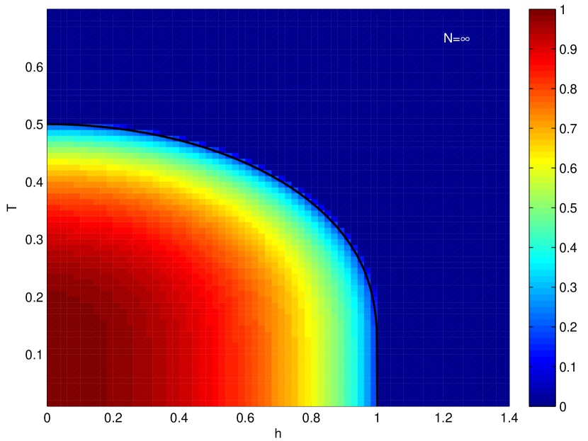
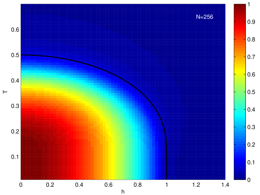
Now that we understand how to do the calculations, let us get a better feeling for the LMG model by looking explicitly at the aforementioned order parameter. It clearly differentiates the two phases, as can be seen from the upper part of figure 6.1 (obtained using the mean-field theory of section 6.3.1): There is the ordered phase for low field and temperature, and the disordered phase elsewhere.
The lower part of figure 6.1 then shows what happens if we do the calculation not by using mean-field theory, but working with a fixed number of spins, using the approach of section 6.3.2. In fact, we numerically calculate the order parameter as in order to avoid any problems due to symmetry-breaking.
For as chosen in the figure we get the same characteristic picture as in the thermodynamic limit, with of course some inevitable finite-size corrections. We can conclude that already gives us a very good idea even if we declare ourselves interested in the behaviour in the thermodynamic limit.
There are two interesting extreme cases of the LMG model that we will specially consider in the following: The left edge of the phase space, , is what we will call the classical limit: Since there is no transverse field, we can work with classical spins (in the -basis). The bottom edge, where , is the zero-temperature limit. The case will usually not be explicitly shown in the plots since, as mentioned, it requires a different (if simpler) algorithm and would just smoothly add another line of barely visible pixels anyway.
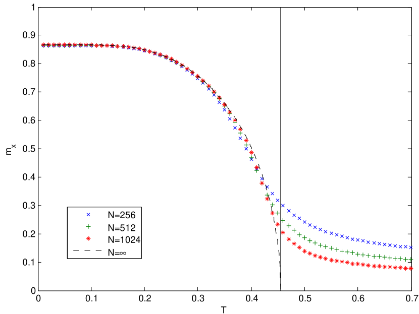
Let us also look at some cross-sections of these plots, in figure 6.2. You can see that (as one would expect) for increasing the thermodynamic limit is approximated better and better. was chosen since it represents a somewhat more general case than e.g. (which looks very similar, only with the transition at ).
6.3.4 Magnetic susceptibility
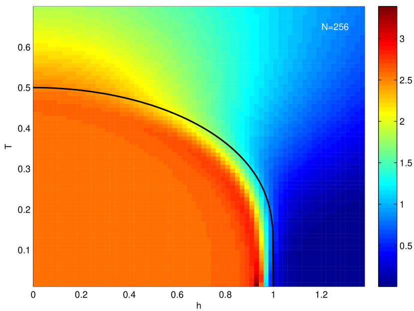
The order parameter gives us a good idea about the two distinct phases, the ordered (ferromagnetic) and disordered (paramagnetic) one. We will however be most interested in the phase transition between those. So are there quantities that show a more “interesting” behaviour at the phase transition than just going to zero as the order parameter does? Maybe the most obvious choice is the magnetic susceptibility, which is just the derivative of our order parameter with respect to the magnetic field, . In the thermodynamic limit, this will diverge at the phase transition. At finite , there is still a pronounced maximum near the phase transition, as can be seen in figure 6.3. While it would still be possible to produce mean-field plots for classical thermodynamic quantities such a the susceptibility, from now on we will mostly stick to finite- plots, since these will be the only thing that we will be able to produce for the more interesting quantities we will study later, at least in the full phase space.
One more thing to say about the susceptibilities: It would also be possible to use not the magnetization in -direction, but rather the magnetization in the direction of the field (or maybe even the total magnetization). These will all result in slightly different plots, but we will not go into that any further, since this is of little relevance to the quantities we will want to study later anyway.
6.3.5 Heat capacity
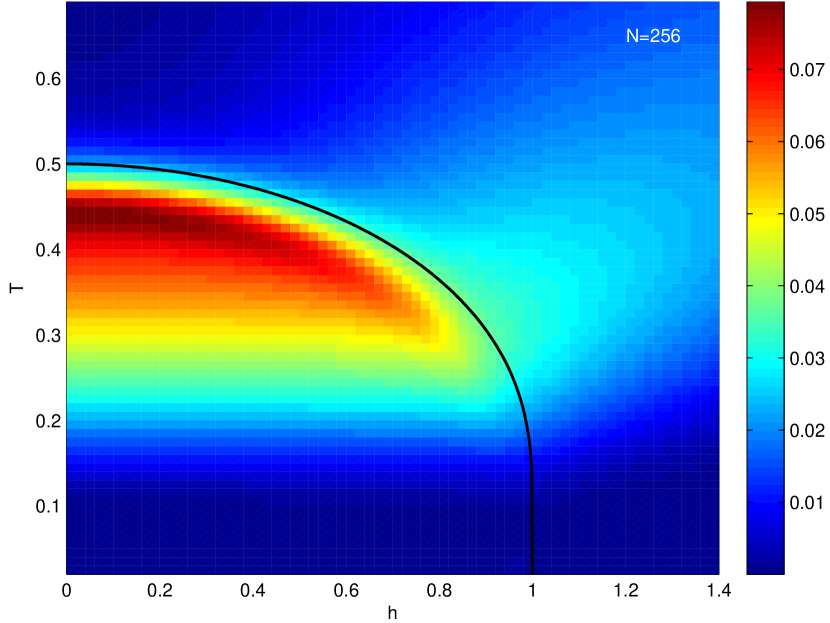
In order to complete the survey of all the “standard” quantities that one thinks of in relation to the study of phase transitions, let us also take a quick look at the heat capacity. In particular, this was also our choice in the classical Ising model on a lattice (where there was no obvious choice of external field, with respect to which one would derive).
The study of the heat capacity is in some way complementary to the study of the order parameter and related magnetic susceptibilities: rather than derive with respect to the magnetic field to arrive at magnetic susceptibilities, we derive with respect to the temperature.
This is somehow evident in the fact that, as figure 6.4 shows, in a colour plot the heat capacity seems to work better as an indicator for the “fully thermal” transition at low fields, and not work quite as well where the external field is relevant. It should however be noted that even there the heat capacity still has a clear maximum near the phase transition; it is just not easily visible in this figure that is trying to show the full transition line at once.
6.4 Finite size scaling properties
We said we wanted to study the behaviour at (or nearby) the phase transition, so what is it that one studies quantitatively in such a situation?
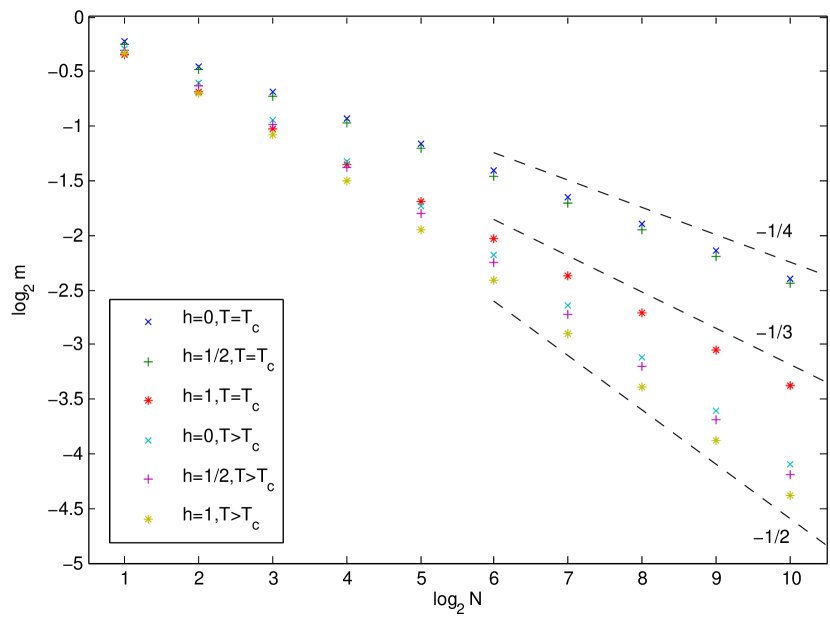
We are dealing with a second-order phase transition, and that implies that there will be critical exponents to be found. So where would we look for such critical exponents? The obvious choice is the order parameter: we can examine how it tends to zero either as a function of , or as a function of the number of spins , at the critical point. The former was already displayed in figure 6.2, and when studying this in more detail one can indeed see that it matches the known critical behaviour: the order parameter goes to zero as with the known critical exponent [96].
What about critical exponents associated to the behaviour as a function of ? As we can also see in figure 6.5, within the disordered phase, i.e. for , the order parameter (which is zero in the thermodynamic limit) vanishes as . You would probably not even call that a critical exponent, but it is important to know in order to compare it to the critical behaviour: At , where the phase transition occurs at a nonzero temperature the order parameter instead behaves as . As you can see, the exact value of is irrelevant for the asymptotic behaviour.
However, the case is special: Here the critical temperature is zero; we are dealing with a quantum phase transition. First of all, this means that a different numerical approach is required. As described in section 6.3.2 however, we can also easily enough access the ground state and calculate its properties, such as the expectation values needed for the order parameter. What we can see is a different critical exponent, with the order parameter going to zero as .
We will be interested in studying such scaling behaviour also for the mutual information, and in particular again contrast finite with zero temperature in section 6.7.
6.5 Entanglement measures
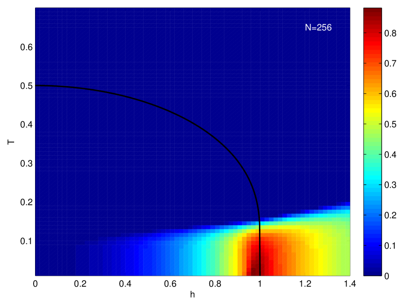
Let us stay with the topic of zero versus finite temperature for a bit: Part of the motivation for looking at mutual information was that it is the generalization of entanglement entropy, which proved useful for pure states, and in particular also for the study of the ground state of the LMG model. While entanglement entropy was not the only entanglement measure that proved interesting there, a general problem with entanglement measures is that many of them only work well for pure states. An exception that remains well-defined for mixed states and can also still be calculated efficiently is concurrence [101], which has indeed already been examined for this model, both at zero [91, 92, 93] and at non-zero temperature [102]. However, take a look at figure 6.6: As you can see, it works well in the vicinity of the quantum phase transition, but has no interesting features at all for most of the finite-temperature transition.
Can we explain why concurrence works so badly? I believe the answer lies in the argument presented in the first chapter: concurrence may qualify as an entanglement measure, but it is not a good measure of all many-body correlations. In fact, it can be calculated from the reduced density matrix of just two spins, and the calculation can even be reduced to a formula involving only expectation values of expressions at most quadratic in spin operators. It is therefore also much easier to calculate than mutual information will prove to be – but even if it seems to work well for the quantum phase transition, it is of little use to us if it does not exhibit any interesting behaviour at finite temperature as well.
Among the other quantities that have been studied in the zero-temperature case for the LMG model, there is one more where the definition straightforwardly generalizes to the finite-temperature case, namely, (logarithmic) negativity [94]. However, the calculation is again significantly more involved, and there is probably little chance of achieving it for thermal states.
6.6 Mutual information
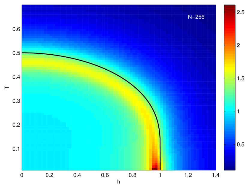
Now let us finally look at mutual information, as promised. Figure 6.7 shows the results; the numerical algorithm will be described in section 6.9. Section 6.10 will show how an analytical approach is possible in the case of vanishing magnetic field the left edge of the plot. As mentioned, this case will also be called the classical limit in the following, since there are no non-commuting observables any more, and everything can be expressed using classical (thermal) probability distributions.
We see that the result is rather convincing: the maximum of the mutual information follows exactly the phase transition. Certainly this is a much more convincing plot than the one shown for concurrence in the previous section, further supporting our arguments from chapter 2 for studying mutual information as a measure of correlations. I also think it is a much nicer plot than either susceptibility (figure 6.3) or heat capacity (figure 6.4).
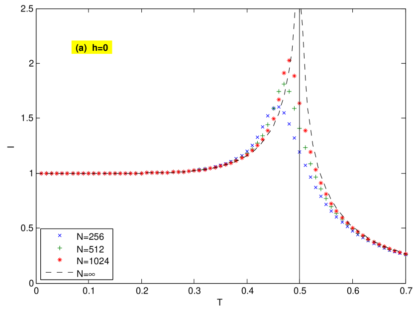
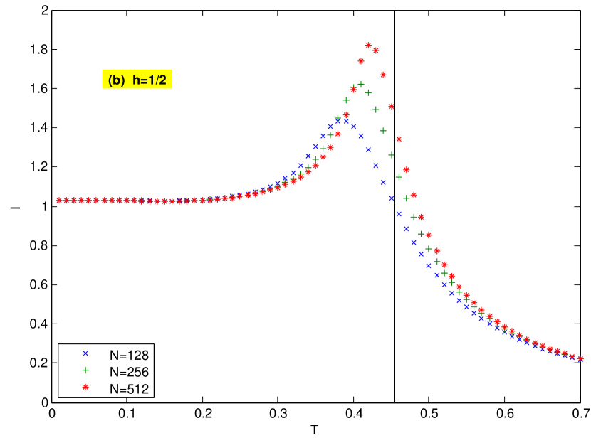
Similarly to what we did in figure 6.2, we can again plot some cross-sections to get a better feeling for the behaviour of the mutual information. Figure 6.8 shows cross-sections for constant magnetic field. Part (a) is for the special case of (which we now call the classical limit), and part (b) shows the rather generic case of .
As you can see, the two cases are actually not very different, but studying the classical limit has two distinct advantages: For one, the numerics actually become much simpler than what is described in section 6.9 for the general case: The Hamiltonian becomes proportional to , and we know that everything becomes diagonal in the -basis, so we just need to deal with classical probability distributions rather than density matrices. In fact, there are just different possible eigenvalues and their degeneracies are easily calculated numerically as binomial coefficients. Of course, we actually need something a bit more complicated than that, splitting the whole system into subsystems and , but it can be written down straightforwardly and easily implemented numerically (which was in this case done in Mathematica, because that allows to calculate binomial coefficients even where it becomes problematic with IEEE754 64-bit arithmetic [70], which was important for the large- studies in section 6.7).
The second advantage is that in this setting, it also becomes possible to do analytical calculations extending to the thermodynamic limit , the result of which is also shown in figure 6.8(a). This is however far more challenging, as outlined in section 6.10. The general idea is to approximate the binomial coefficients (along the lines of Stirling’s formula), replace sums by integrals, and approximate those integrals. For the plot in figure 6.8(a), however, numerical evaluation of the resulting integrals was in fact sufficient.
6.7 Scaling behaviour and comparison to the QPT
Can we extract more predictions about the mutual information from the analytical treatment of the classical case in section 6.10? In fact, after a lot of calculation we find a very nice critical scaling of the mutual information (compare equation (6.19)):
We can call the coefficient a critical exponent, just like the exponents we found when studying the order parameter in section 6.4.
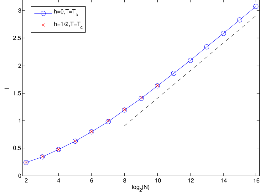
Let us first check if our numerical simulations match the analytical calculation. Figure 6.9 shows that this is indeed very much the case. In particular the agreement for is very good for the larger we can access numerically in this case, as explained in the previous section. For a non-zero , like the displayed here, we cannot access quite such large system sizes, but as you can see, the mutual information is almost identical for those system sizes that we can access.
Of course this changes considerably if we get very close to the quantum phase transition at . Remember that there also the order parameter showed a different critical exponent, of rather than . Do you want to predict what happens for the mutual information?
Since at zero temperature, mutual information is just twice the entanglement entropy, its scaling behaviour has already been carefully studied in [37, 38, 39, 40], and in fact it has been found analytically that the entanglement entropy behaves like , and the mutual information therefore as 111The initial numerical study [37] mistakenly identified the scaling behaviour of the entanglement entropy as . The later references contain the correct result.. This parallel between the behaviour of the order parameter and the mutual information does in fact seem extraordinarily nice.
6.8 From Ising to XY
So far, we considered the special case of a zero in (6.1). What happens for nonzero (which we could now maybe call an anisotropy parameter)? This corresponds to going from a pure Ising- to an XY-type model of competing - and -interactions; there is now no classical limit anymore, but our numerical procedure as described in section 6.9 remains applicable.
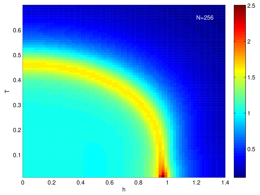
Figure 6.10 shows some results for , and in fact not much seems to have changed. However, there is one rather nice additional feature: If you look carefully at low temperatures and around , you notice that the mutual information seems to be a bit lower there than at both lower and higher . This is much better visible in figure 6.11, which plots exactly the same data, but this time only a few relevant cross-sections at fixed low values of .
In fact, this behaviour is a signature of the two-fold degenerate and separable ground state at [93, 39, 105], so for our choice of this occurs at . We can call this a “Kurmann point”, and see that the mutual information (where we put in absolutely no knowledge of such behaviour) gives us a good idea of how this effect still remains visible at non-zero temperatures.
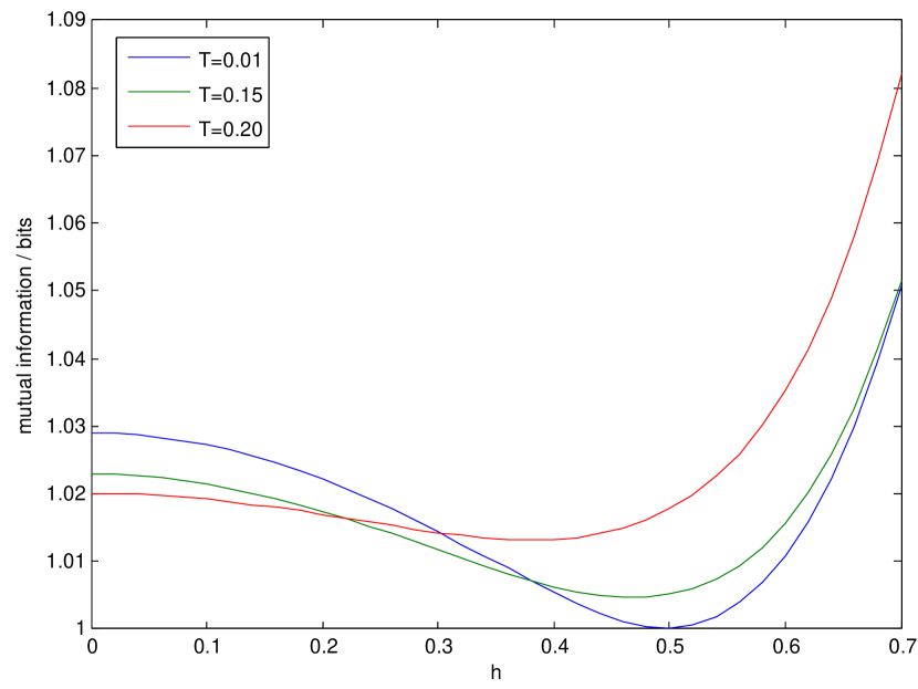
What happens if we go all the way towards the case of an interaction that is isotropic in and ? The results are shown in figure 6.12. Clearly, this is quite a different picture now! The essential difference is that the Hamiltonian now has an additional symmetry; it is isotropic in the --plane. This changes the universality class, and explains why is qualitatively so different from the and cases (both of which are anisotropic and generally pretty similar). This has been studied in the ground state case in the aforementioned references [91, 92, 93, 94, 37, 38, 39, 40]. It will however be a challenge to make any analytical statements about the thermal case, especially as there is now no classical limit any more.
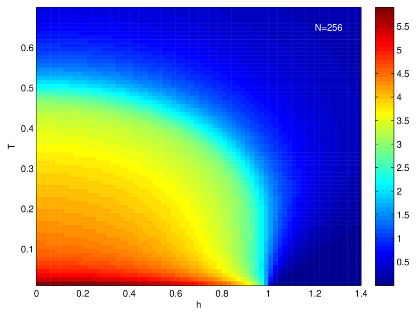
Let us also use this opportunity to point out that our methods give us access not only to the mutual information, but really to the full spectrum of the reduced density matrices from which it is calculated. These “entanglement spectra”, where the eigenvalues of the reduced density matrices are studied, typically sorted by a good quantum number such as the total angular momentum in the subsystem, have received some attention in recent years [106, 107, 108, 109]. Unfortunately, there does not currently seem to be much theory that we can compare the entanglement spectra of our models to. Nevertheless, figure 6.13 presents some finite-temperature entanglement spectra which show that not only the mutual information, but also the spectra themselves are significantly different between the and cases.
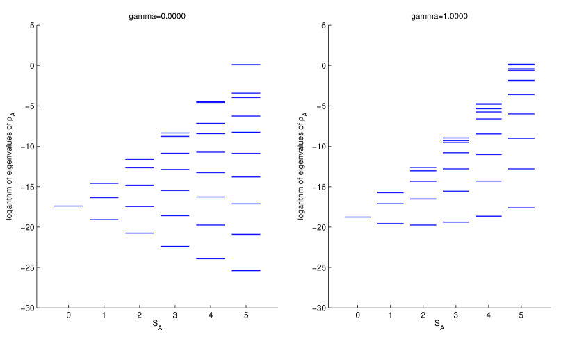
6.9 Algorithm for calculating mutual information in spin-conserving Hamiltonians
Let us now give the algorithm we used for numerically calculating the mutual information, as also presented in [2]. It works for any Hamiltonian fulfilling the essential property . In section 6.3.2, we saw how to calculate the partition function using the block decomposition of such a Hamiltonian while keeping track of multiplicities. With all the spin quantum numbers, there will now be a lot of instances of the letter around. To avoid confusion, let us therefore use a different letter for the entropies, namely, Just like we did for the partition function before, in equation (6.5), we can now write the (total) entropy as
| (6.6) |
where is the density matrix and where we defined and .
Computation of and
The much more challenging part is the calculation of entropies of the subsystems in our definition of the mutual information (2.1). We split the system into two subsystems and containing and spins respectively, and aim to compute the entropies of the reduced density matrices and .
Again, the essential idea is to work with a block decomposition of the Hamiltonian, and density matrix. However, what makes this more challenging now is that we have to be able to take partial traces, which means we need a basis with a tensor product structure. Therefore, we cannot straightforwardly work with the total spin. However, what we can do instead is combine the spins in and separately, to total spins which we can label and . The most straightforward thing would then be to work in the basis of states
where the s label e.g. the -component of the respective spins. In this basis, taking partial traces is straightforward (although we would still need to keep track of all multiplicities). However, this is not the most efficient approach, because this forces us to work with much bigger blocks which arise in the tensor product basis.
It is more efficient to couple and to a total spin again and work with the density matrix in the blocks of fixed In order to calculate partial traces, we will then need to work with Clebsch-Gordan coefficients describing the angular momentum coupling. However, this can be done rather efficiently. While this basic idea is simple enough, the formulas will unfortunately start to look rather messy, due to the fact that not every and can be coupled to every . Let us start with the Hamiltonian, which reads
where denotes an eigenstate of operators and with eigenvalues , , and respectively. Index () labels the () degenerate subspaces of spin () that can be built from () spins 1/2. For a given , primed sums are restricted to values of and that can add to a total spin . That is to say, one must fulfill the inequalities , so one can alternatively write:
We have denoted as , and the maximum spins of the whole system and of each of the subsystems. As before, minimum spins are denoted with square brackets. Note that the degeneracy of the spin- sector can be recovered from
The matrix elements are the same as in formula (6.2), and do not depend on , , or . Therefore, all Hamiltonians have the same eigenvalues (which are the same as in equation (6.3)), and corresponding eigenvectors
Once again, coefficients are independent of , , and , and are the same as in equation (6.4).
Now, the density matrix reads
where denotes the complex conjugate of .
Now we have to decompose each basis state into the tensor product state basis using Clebsch-Gordan coefficients
with obvious notations. The only pairs that contribute to the above sum are such that , since the Clebsch-Gordan coefficients vanish otherwise. Introducing the shorthand notation
we get
| (6.7) |
It is now possible to perform the partial traces. Let us focus on computing . This partial trace will enforce in . Furthermore, the index disappears from the quantity to be summed over, so that simply yields a factor . At the end of the day, one finds
| (6.8) | |||||
with
These limits come from the fact that not all values of are allowed in between and , but only those that fulfill and . Let us remark that, here, we have got rid of the sum over and kept the sum over . One could have of course done the opposite, resulting in a somewhat different implementation.
Expression (6.8) of allows one to numerically compute . The partial entropy can be computed similarly. We already saw in formula (6.6). Once we have all of these, the mutual information is simply obtained from its definition (2.1).
It should be noted that the above algorithm requires the numerical computation of many Clebsch-Gordan coefficients. To see why that is important, let us estimate the computational complexity of our algorithm. Looking at equation (6.8), one sees that eight sums are involved. However, the sum over will only yield a multiplicity, which leaves seven sums. Furthermore, the matrices created by the sum over (which is enclosed in parentheses above)
can be computed once (for all the different values of ), and stored in memory. These matrices are nothing but the density matrices in the spin- sectors (up to a factor of ). The computational cost of this is comparatively negligible, and one is left with a sum over six variables, namely , , , , and , which all take a number of values scaling linearly with (at most). So we expect that our algorithm roughly scales as in computation time. However, there we made an important assumption, namely that we already know the Clebsch-Gordon coefficients. Indeed, if we count them, we realize that we actually need in the order of different ones of them. That means we need a very efficient way of calculating them, otherwise this becomes the bottleneck of the algorithm. In fact, even calculating all the coefficients for a given system size in advance and storing them is not attractive: we would require a huge amount of storage and reading from such storage would not be very fast.
It is however indeed possible to calculate Clebsch-Gordon coefficients efficiently, with just a small and constant number of operations per coefficient. To do this, one needs to calculate them recursively. However, the required recursion has nontrivial stability properties; it is only stable in some of the possible directions, otherwise numerical inaccuracies pile up very quickly. In the end, we arrived at the same algorithm as is also described by Schulten and Gordon [110].
6.10 Analytical calculations in the classical limit
In this section (which has been relegated to the end of the chapter like the previous one, in order not to interrupt the discussion of results), let us understand the analytical treatment of the classical (quantum fluctuation free) case . In this case, the LMG Hamiltonian (6.1) simplifies to
Its eigenstates are now those of , and can be chosen as separable states , with spins pointing in the direction and spins pointing in the direction. The variable allows to distinguish between the such states which are degenerate and have eigenenergy .
To obtain the mutual information, again one first needs to compute the total entropy of the system at finite temperature. Let us again start with the partition function
| (6.9) |
where as before, denotes the inverse temperature . Despite the apparent simplicity of , it is difficult to compute analytically for arbitrary finite . That is why we will now focus on the physically relevant large- limit to analyze the thermodynamical limit and its neighbourhood. Computations get easier in this limit because the discrete sum in (6.9) can be approximated by an integral with, as is well-known, an error of the order . This is fortunate since, in order to compute the mutual information in the present problem, we will need to compute the first correction to the infinite limit.
The very first step in the calculation is to perform a large- expansion of the binomials
| (6.10) |
Using the series expansion of the Euler function at large (or the Stirling formula) and skipping terms of relative order , one gets
| (6.14) | |||||
where we set . Then, replacing the sum by an integral in equation (6.9) gives
Furthermore, the exponential term allows us to extend the integration range to . Indeed, the effect of this extension consists in exponentially small terms ) which are negligible compared to the error we already made by approximating the sum by an integral. The resulting integral can be evaluated using the standard Laplace’s method (also known as saddle-point or stationary-phase approximation) though one has to take care of computing the subleading corrections [111].
At and above the critical temperature (), the minimum of is found for and the result of the saddle-point approximation reads
| (6.15) |
and
Note that, in this approach, does not coincide with (which is divergent) since the integral arising from the saddle-point approximation is not Gaussian anymore at criticality. Furthermore, we see that diverges with a non-trivial finite-size scaling exponent, as . This result, which is obtained by directly computing , is consistent with equation (6.15). Indeed, adapting the finite-size scaling argument developed in references [92, 93] for the zero-temperature problem, one can write (for smaller than but close to 2) where is the thermodynamical limit value of , and is a scaling function. As this quantity cannot be singular for finite , one must have so that the singularity at disappears : .
In the low-temperature phase (), has two symmetric minima, the position of which can only be computed numerically. Once determined, one can still perform the Gaussian integral resulting from the second-order Taylor expansion around these minima, which yields a “numerically exact" result in the infinite- limit. As a consequence, we only give analytical expressions for , but we can still obtain exact numerical results for , as we saw e.g in figure 6.8(a).
To compute the entropy in the thermodynamical limit, let us start by computing the internal energy of the system using the same approximation (6.14) of the binomials. The internal energy is
where is the thermal density matrix. For , it can be obtained from equation (6.15) but, as before, special care must be taken to deal with the critical case for which one can show that
so that the internal energy diverges as .
The desired entropy can now be computed (analytically for and numerically for ) as
| (6.17) |
Computing the mutual information is still a challenge, the most difficult part of which lies in the derivation of the large- behavior of the subsystem entropies like
where is the reduced density matrix (and correspondingly for subsystem ). It is therefore mandatory to find an expression for (and ). With this aim in mind, let us split the system into two parts and containing and spins respectively. Next, let us decompose the eigenstates of as with and where denotes a state of subsystem that has spins pointing in the direction. Variable can take values, describing which spins point in the direction. This decomposition allows one to write the reduced density matrix as
Here, we introduced the quantity
The subsystem entropy is then
Following the same line of reasoning as for the partition function calculation and replacing the binomials by the same form as (6.14), one can again use Laplace’s method to obtain the large- behavior of the partial entropy. Things are now rather more involved since one has to deal with a double sum and therefore with a two-variable integral. After some algebra, we get
and
where we have identified , and .
Finally, noting that is obtained from by exchanging and using (6.17), one obtains the following expressions of the mutual information
| (6.18) |
and
| (6.19) |
Chapter 7 -models
In this chapter, we will consider a class of generalizations of the Lipkin-Meshkov-Glick model that was discussed in the previous chapter. Again, the ground state entanglement properties of these models have received some attention recently [112]. We will now examine what happens in the finite-temperature case.
7.1 Hamiltonians
Let us consider the Hamiltonian
where
These values have been chosen such that the relevant parameter range for is always and the zero-temperature phase transition always occurs exactly in the middle of it, at .
In particular, the case is again our LMG model in a slightly re-parametrized form. We can consider the other cases generalizations of the LMG model, in the sense that when we imagine the model derived from spin- particles again, they describe interactions between not just two spins, but or spins each instead. What is important is that in every case the all-essential property is preserved, and therefore the numerical methods of section 6.9 still remain applicable. In fact, even more symmetries are preserved: the spin-flip symmetry in -direction still exists in the cases where is even, and there occurs a corresponding spin-flip symmetry in -direction for even .
7.2 Calculating the location of the phase transition
We are of course again mainly interested in the behaviour of the mutual information in the vicinity of the phase transition. For this, we first have to know where exactly the phase transition is located. It is in principle straightforward to generalize the procedure used in the Lipkin model to higher spins; however, the equations become significantly more complicated. In particular, there are in general many more possible solutions for the magnetization and it will now be much more important to check which possible solution for the magnetization has the lowest free energy. It becomes very hard to write down analytical solutions, but since we have no particular interest in the analytical form anyway, we can just implement it numerically, which is possible without problems. Let us recall all the steps from the LMG case and see where things are different.
Again, we start by introducing order parameters , and now also . The mean field approach is just the same as in section 6.3.1, replacing and in the Hamiltonian, ignoring quadratic and higher terms in the “deviations” and . This again yields a Hamiltonian of the form
which consists of a linearly spin-dependent part with
and a part that involves only the mean-field magnetizations ,
Again, we demand self-consistency as before, and find the mean-field magnetizations (order parameters) as the self-consistent solution that has the lowest free energy. The actual equations become rather messy but can be handled efficiently numerically.
A phase transition occurs wherever an infinitesimal change of parameters makes at least one of the order parameters change from zero to some finite value, which can also easily be determined numerically.
7.3 First order versus continuous (second order) phase transition
In the LMG model, we were dealing with a continuous phase transition. This was manifesting in the fact that the order parameter went from zero to a finite value in a continuous manner; this continuity does not, however, extend to derivatives [113].
However, many of the --models we will now study do not exhibit such a continuous (sometimes still called second-order) transition. Instead the order parameter is discontinuous at the phase transition, as shown for the (3,1)-model in figure 7.1. It is therefore also quite impossible to define anything like critical exponents – there is no universal behaviour for such first-order transitions.
In the next section we will see that the behaviour of the mutual information will also be very different in those models that show a first-order transition rather than a continuous one.
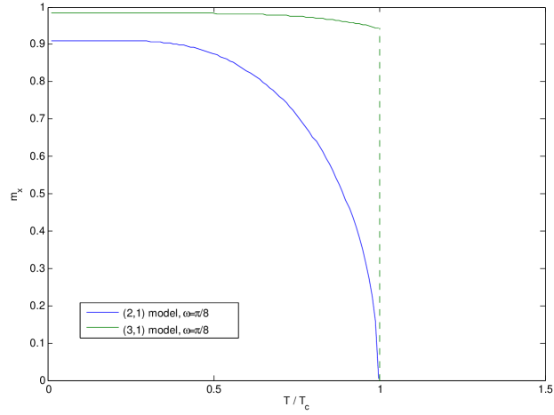
7.4 Results
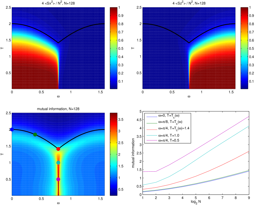
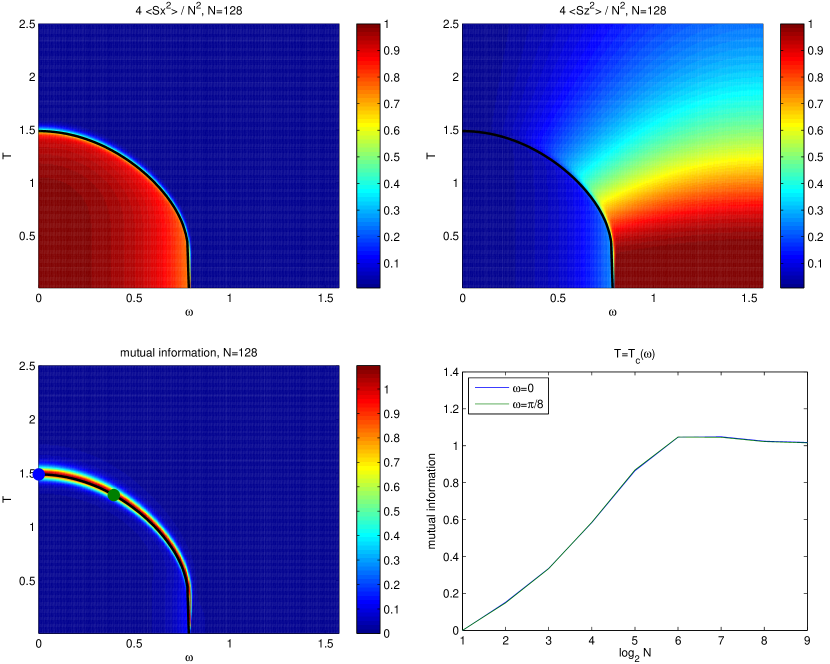
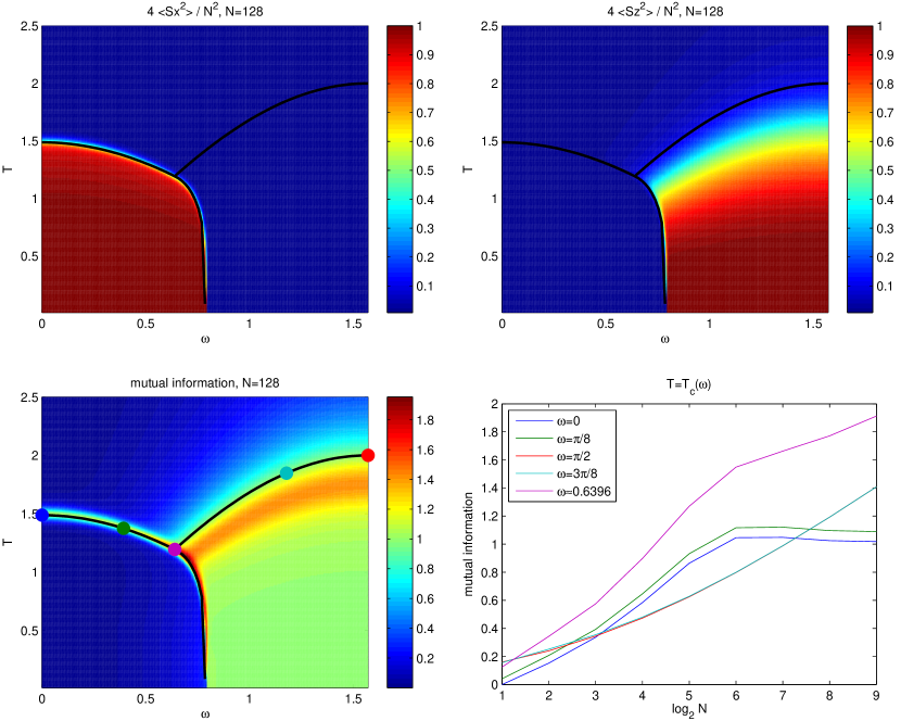
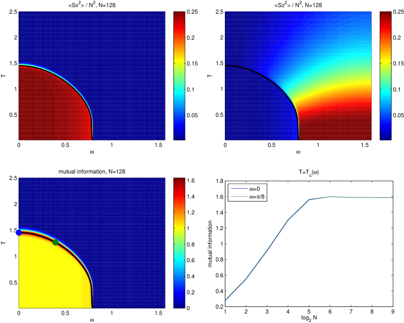
As mentioned, the LMG model is equivalent to the (2,1)-model. Since it has been studied extensively in the previous chapter, we just remember that we got a good idea about its phase diagram by looking at the order parameter in figure 6.1. Since we can now also have an interaction in -direction, we will for the new models also plot the corresponding order parameter . As in section 6.3.3, we calculate the order parameters using and to avoid any confusion by symmetry-breaking.
The essential behaviour that we found for the mutual information in the LMG model was displayed in figure 6.7, where you can see how it beautifully follows the phase transition, and in the thermodynamic limit diverges logarithmically at the critical temperature, as was examined in figure 6.9.
We will therefore now be studying the same sort of plots for the (2,2)-, (3,1)-, (3,2)-, and (4,1)-models. The numerically determined locations of the phase transitions will be marked by solid black lines.
The Hamiltonian is clearly symmetric in and , so that e.g. the (2,3)-model is exactly the same as the (3,2)-model. It also turns out that models with even higher and will not show any interesting new features, which is why we restrict ourselves to this selection. Since some of the density plots will need finer resolution (i.e., more data points) than those in the last chapter, we reduced the system sizes we studied to , in order to speed up computations.
What do we find? The particular observations for each model are noted in the caption below it, so let us just summarize the general behaviour here: only a two-spin-interaction gives rise to a continuous phase transition, where the mutual information diverges logarithmically.
Higher-order interactions still give rise to distinct phases, but with a first-order transition between them, which shows up as much sharper in the plots. In fact the mutual information captures also this type of phase transition very well. However, one would not expect any critical behaviour, and the mutual information shows none, it just goes to a constant value.
Again, this sort of comparably trivial behaviour in the first-order transitions corresponds with what has been found for the quantum phase transitions in the same models in [112], where in particular the entanglement entropy has been found to diverge only in continuous transitions.
Concluding remarks and outlook
I hope that I have managed convince you that mutual information is interesting! We have seen that is a well-founded correlation measure. It is not easy to calculate though – the biggest parts of this thesis were dedicated to the problems of calculating it, in what are after all rather simple model systems. I think it was worth the effort though: We have clearly seen that mutual information has pronounced features around a phase transition – be it in the classical spin systems on a lattice or in the fully-connected models. In the latter, we even saw analytical results that support the argument that it is a natural generalization of entanglement entropy.
For the systems studied, I certainly would not claim that it is very useful for detecting the phase transitions, because these systems are rather well understood and there are far easier ways to find their phase transitions. We can however extract more information than just the location of the phase transition – we also learn about the amount of correlations in the different phases and at the transition between them: remember for example the Kurmann point in section 6.8 and the markedly different behaviour at first- and second-order phase transitions we saw in chapter 7. Most crucially, we get all this without having needed any intuition about order parameters. That means such information-theory-based methods immediately suggest themselves for the study of any sort of novel phases, which are not yet as well-understood – similarly as entanglement entropy has turned out essential for ground-state studies in topological models [115, 116]. Of course that will in general be even more challenging, but I think we have so far only seen a very small part of what is possible at the point where (quantum) information theory and condensed matter intersect.
References
- [1] J. Wilms, M. Troyer, and F. Verstraete. Mutual information in classical spin models. Journal of Statistical Mechanics: Theory and Experiment, 2011:P10011, 2011.
- [2] J. Wilms, J. Vidal, F. Verstraete, and S. Dusuel. Finite-temperature mutual information in a simple phase transition. Journal of Statistical Mechanics: Theory and Experiment, 2012:P01023, 2012.
- [3] V. Vedral, M. B. Plenio, M. A. Rippin, and P. L. Knight. Quantifying entanglement. Phys. Rev. Lett., 78:2275–2279, 1997.
- [4] T. M. Cover and J. A. Thomas. Elements of Information Theory. Wiley, 1991.
- [5] C. E. Shannon. A mathematical theory of communication. The Bell System Technical Journal, 27:379, 1948.
- [6] M. A. Nielsen and I. L. Chuang. Quantum Computation and Quantum Information. Cambridge University Press, 2000.
- [7] N. J. Cerf and C. Adami. Negative entropy and information in quantum mechanics. Physical Review Letters, 79(26):5194–5197, 1997.
- [8] A. Rényi. On measures of entropy and information. In Proceedings of the 4th Berkeley Symposium on Mathematics, Statistics and Probability, page 547, 1961.
- [9] A. Rényi. On the foundations of information theory. Revue de l’Institut International de Statistique, pages 1–14, 1965.
- [10] P. Viola and W. M. Wells III. Alignment by maximization of mutual information. International Journal of Computer Vision, 24(2):137–154, 1997.
- [11] P. Viola. Alignment by maximization of mutual information. PhD thesis, Massachusetts Institute of Technology, 1995.
- [12] W. M. Wells III, P. Viola, H. Atsumi, S. Nakajima, and R. Kikinis. Multi-modal volume registration by maximization of mutual information. Medical Image Analysis, 1(1):35–51, 1996.
- [13] A. Collignon, F. Maes, D. Delaere, D. Vandermeulen, P. Suetens, and G. Marchal. Automated multi-modality image registration based on information theory. In Information Processing in Medical Imaging, volume 3, pages 264–274, 1995.
- [14] A. Collignon. Multi-modality medical image registration by maximization of mutual information. PhD thesis, Catholic University Leuven, Leuven, Belgium, 1998.
- [15] A. M. Fraser and H. L. Swinney. Independent coordinates for strange attractors from mutual information. Physical Review A, 33(2):1134, 1986.
- [16] J. B. Michel, Y. K. Shen, A.P. Aiden, A. Veres, M. K. Gray, J. P. Pickett, D. Hoiberg, D. Clancy, P. Norvig, J. Orwant, et al. Quantitative analysis of culture using millions of digitized books. Science, 331(6014):176, 2011.
- [17] H. Matsuda, K. Kudo, R. Nakamura, O. Yamakawa, and T. Murata. Mutual information of Ising systems. International Journal of Theoretical Physics, 35(4):839–845, 1996.
- [18] R. V. Solé, S. C. Manrubia, B. Luque, J. Delgado, and J. Bascompte. Phase transitions and complex systems. Complexity, 1(4):13, 1996.
- [19] D. V. Arnold. Information-theoretic analysis of phase transitions. Complex Systems, 10:143, 1996.
- [20] M. B. Hastings, I. Gonzalez, A. B. Kallin, and R. G. Melko. Measuring Rényi entanglement entropy in Quantum Monte Carlo simulations. Physical Review Letters, 104:157201, 2010.
- [21] R. G. Melko, A. B. Kallin, and M. B. Hastings. Finite-size scaling of mutual information in Monte Carlo simulations: Application to the spin-1/2 XXZ model. Physical Review B, 82:100409, 2010.
- [22] R. R. P. Singh, M. B. Hastings, A. B. Kallin, and R. G. Melko. Finite-temperature critical behavior of mutual information. Physical Review Letters, 106:135701, 2011.
- [23] R. Renner and S. Wolf. Smooth Rényi entropy and applications. In International Symposium on Information Theory, 2004. Proceedings, 2004.
- [24] R. König, R. Renner, and C. Schaffner. The operational meaning of min- and max-entropy. IEEE Trans. Inf. Theory, 55:4337, 2009.
- [25] R. V. L. Hartley. Transmission of information. The Bell System Technical Journal, 7:535, 1928.
- [26] M. M. Wolf, F. Verstraete, M. B. Hastings, and J. I. Cirac. Area laws in quantum systems: mutual information and correlations. Physical Review Letters, 100(7):70502, 2008.
- [27] G. Vidal, J. I. Latorre, E. Rico, and A. Kitaev. Entanglement in quantum critical phenomena. Physical Review Letters, 90(22):227902, 2003.
- [28] P. Calabrese and J. Cardy. Entanglement entropy and quantum field theory. Journal of Statistical Mechanics: Theory and Experiment, 2004:P06002, 2004.
- [29] M. B. Plenio, J. Eisert, J. Dreissig, and M. Cramer. Entropy, entanglement, and area: analytical results for harmonic lattice systems. Physical Review Letters, 94(6):60503, 2005.
- [30] A. R. Its, B. Q. Jin, and V. E. Korepin. Entanglement in the XY spin chain. Journal of Physics A: Mathematical and General, 38:2975, 2005.
- [31] F. Verstraete and J. I. Cirac. Matrix product states represent ground states faithfully. Physical Review B, 73(9):94423, 2006.
- [32] F. Verstraete, M. M. Wolf, D. Perez-Garcia, and J. I. Cirac. Criticality, the area law, and the computational power of projected entangled pair states. Physical Review Letters, 96(22):220601, 2006.
- [33] M. B. Hastings. An area law for one-dimensional quantum systems. Journal of Statistical Mechanics: Theory and Experiment, 2007:P08024, 2007.
- [34] J. Eisert, M. Cramer, and M. B. Plenio. Colloquium: Area laws for the entanglement entropy. Reviews of Modern Physics, 82:277–306, 2010.
- [35] J. M. Stéphan, S. Furukawa, G. Misguich, and V. Pasquier. Shannon and entanglement entropies of one-and two-dimensional critical wave functions. Physical Review B, 80(18):184421, 2009.
- [36] J. M. Stéphan, G. Misguich, and V. Pasquier. Rényi entropy of a line in two-dimensional ising models. Physical Review B, 82(12):125455, 2010.
- [37] J. I. Latorre, R. Orús, E. Rico, and J. Vidal. Entanglement entropy in the Lipkin-Meshkov-Glick model. Physical Review A, 71:064101, 2005.
- [38] T. Barthel, S. Dusuel, and J. Vidal. Entanglement entropy beyond the free case. Physical Review Letters, 97:220402, 2006.
- [39] J. Vidal, S. Dusuel, and T. Barthel. Entanglement entropy in collective models. Journal of Statistical Mechanics: Theory and Experiment, 2007.
- [40] R. Orús, S. Dusuel, and J. Vidal. Equivalence of critical scaling laws for many-body entanglement in the Lipkin-Meshkov-Glick model. Physical Review Letters, 101:025701, 2008.
- [41] N. Metropolis, A. W. Rosenbluth, M. N. Rosenbluth, A. H. Teller, and E. Teller. Equation of state calculations by fast computing machines. The Journal of Chemical Physics, 21:1087, 1953.
- [42] D. P. Landau and K. Binder. A guide to Monte Carlo simulations in statistical physics. Cambridge University Press, 2005.
- [43] F. Verstraete, V. Murg, and J. I. Cirac. Matrix product states, projected entangled pair states, and variational renormalization group methods for quantum spin systems. Advances in Physics, 57(2):143–224, 2008.
- [44] B. Pirvu, V. Murg, J. I. Cirac, and F. Verstraete. Matrix product operator representations. New Journal of Physics, 12:025012, 2010.
- [45] H. A. Kramers and G. H. Wannier. Statistics of the two-dimensional ferromagnet. Part I. Physical Review, 60:252–262, 1941.
- [46] H. A. Kramers and G. H. Wannier. Statistics of the two-dimensional ferromagnet. Part II. Physical Review, 60(3):263–276, 1941.
- [47] L. Onsager. Crystal statistics. I. A two-dimensional model with an order-disorder transition. Physical Review, 65(3-4):117, 1944.
- [48] R. J. Baxter. Exactly solved models in statistical mechanics. Academic Press London, 1982.
- [49] T. Nishino. Density matrix renormalization group method for 2D classical models. Journal of the Physical Society of Japan, 64(10):3598–3601, 1995.
- [50] T. Nishino and K. Okunishi. Product wave function renormalization group. Journal of the Physical Society of Japan, 64(11):4084–4087, 1995.
- [51] B. Pirvu, F. Verstraete, and G. Vidal. Exploiting translational invariance in Matrix Product State simulations of spin chains with periodic boundary conditions. Physical Review B, 83(12):125104, 2011.
- [52] A. W. Sandvik and G. Vidal. Variational quantum Monte Carlo simulations with tensor-network states. Physical Review Letters, 99(22):220602, 2007.
- [53] N. Schuch, M. M. Wolf, F. Verstraete, and J. I. Cirac. Simulation of quantum many-body systems with strings of operators and Monte Carlo tensor contractions. Physical Review Letters, 100(4):40501, 2008.
- [54] E. Ising. Beitrag zur Theorie des Ferromagnetismus. Zeitschrift für Physik, 31(1):253–258, 1925.
- [55] L. G. Valiant. Quantum circuits that can be simulated classically in polynomial time. SIAM Journal on Computing, 31:1229, 2002.
- [56] E. Knill. Fermionic linear optics and matchgates. Arxiv preprint quant-ph/0108033, 2001.
- [57] B. M. Terhal and D. P. DiVincenzo. Classical simulation of noninteracting-fermion quantum circuits. Physical Review A, 65(3):032325, 2002.
- [58] S. Bravyi and A. Kitaev. Fermionic quantum computation. Annals of Physics, 298(1):210–226, 2002.
- [59] S. Bravyi. Lagrangian representation for fermionic linear optics. Quantum Information & Computation, 5(3):216–238, 2005.
- [60] R. Jozsa and A. Miyake. Matchgates and classical simulation of quantum circuits. Proceedings of the Royal Society A: Mathematical, Physical and Engineering Science, 464(2100):3089–3106, 2008.
- [61] M. van den Nest, W. Dür, R. Raussendorf, and H. J. Briegel. Quantum algorithms for spin models and simulable gate sets for quantum computation. Physical Review A, 80(5):52334, 2009.
- [62] R. Jozsa, B. Kraus, A. Miyake, and J. Watrous. Matchgate and space-bounded quantum computations are equivalent. Proceedings of the Royal Society A: Mathematical, Physical and Engineering Science, 466(2115):809–830, 2010.
- [63] G. C. Wick. The evaluation of the collision matrix. Physical Review, 80(2):268–272, 1950.
- [64] E. Majorana. Teoria simmetrica dell elettrone e del positrone. Nuovo Cimento, 14(4):171–184, 1937.
- [65] B. M. McCoy and T. T. Wu. The two-dimensional Ising model. Harvard University Press, 1973.
- [66] M. E. Fisher. On the dimer solution of planar Ising models. Journal of Mathematical Physics, 7:1776, 1966.
- [67] M. E. Fisher. Statistical mechanics of dimers on a plane lattice. Physical Review, 124(6):1664, 1961.
- [68] P. W. Kasteleyn. The statistics of dimers on a lattice:: I. the number of dimer arrangements on a quadratic lattice. Physica, 27(12):1209–1225, 1961.
- [69] H. N. V. Temperley and M. E. Fisher. Dimer problem in statistical mechanics-an exact result. Philosophical Magazine, 6(68):1061–1063, 1961.
- [70] IEEE Standard for Floating-Point Arithmetic. Technical report, Microprocessor Standards Committee of the IEEE Computer Society, 2008.
- [71] C. M. Fortuin and P. W. Kasteleyn. On the random-cluster model: I. Introduction and relation to other models. Physica, 57(4):536–564, 1972.
- [72] R. H. Swendsen and J. S. Wang. Nonuniversal critical dynamics in Monte Carlo simulations. Physical Review Letters, 58(2):86–88, 1987.
- [73] F. Albuquerque et al. (ALPS collaboration). The ALPS project release 1.3: open source software for strongly correlated systems. Journal of Magnetism and Magnetic Materials, 310:1187, 2007.
- [74] M. Troyer, B. Ammon, and E. Heeb. Parallel object oriented Monte Carlo Simulations. Lecture Notes in Computer Science, 1505:191, 1998.
- [75] R. B. Potts. The Mathematical Investigation of Some Cooperative Phenomena. PhD thesis, University of Oxford, 1951.
- [76] R. B. Potts. Some generalized order-disorder transformations. Mathematical Proceedings of the Cambridge Philosophical Society, 48(01):106–109, 1952.
- [77] F. Y. Wu. The Potts model. Reviews of Modern Physics, 54(1):235–268, 1982.
- [78] J. Tobochnik. Properties of the q-state clock model for q=4, 5, and 6. Physical Review B, 26(11):6201–6207, 1982.
- [79] J. Tobochnik. Erratum: Properties of the q-state clock model for q=4, 5, and 6. Physical Review B, 27(11):6972, 1983.
- [80] M. S. S. Challa and D. P. Landau. Critical behavior of the six-state clock model in two dimensions. Physical Review B, 33(1):437–443, 1986.
- [81] D. D. Betts. The exact solution of some lattice statistics models with four states per site. Canadian Journal of Physics, 42(8):1564–1572, 1964.
- [82] M. Suzuki. Solution of Potts Model for Phase Transition. Progress of Theoretical Physics, 37:770–772, 1967.
- [83] H. J. Lipkin, N. Meshkov, and A. J. Glick. Validity of many-body approximation methods for a solvable model: (I). Exact solutions and perturbation theory. Nuclear Physics, 62:188, 1965.
- [84] N. Meshkov, A. J. Glick, and H. J. Lipkin. Validity of many-body approximation methods for a solvable model: (II). Linearization procedures. Nuclear Physics, 62:199, 1965.
- [85] A. J. Glick, H. J. Lipkin, and N. Meshkov. Validity of many-body approximation methods for a solvable model: (III). Diagram summations. Nuclear Physics, 62:211, 1965.
- [86] S. Stigler. Stigler’s law of eponymy. In T. F. Gieryn, editor, Science and social structure: a festschrift for Robert K. Merton. New York Academy of Sciences, 1980.
- [87] S. Fallieros. Collective oscillations in O-16. PhD thesis, University of Maryland, 1959.
- [88] J. A. Maruhn, P. Reinhard, and E. Suraud. Simple Models of Many-Fermion Systems. Springer, 2010.
- [89] J. I. Cirac, M. Lewenstein, K. Mølmer, and P. Zoller. Quantum superposition states of bose-einstein condensates. Physical Review A, 57:1208–1218, 1998.
- [90] J. Larson. Circuit QED scheme for the realization of the Lipkin-Meshkov-Glick model. Europhysics Letters, 90:54001, 2010.
- [91] J. Vidal, G. Palacios, and R. Mosseri. Entanglement in a second order quantum phase transition. Physical Review A, 69:022107, 2004.
- [92] S. Dusuel and J. Vidal. Finite-size scaling exponents of the Lipkin-Meshkov-Glick model. Physical Review Letters, 93:237204, 2004.
- [93] S. Dusuel and J. Vidal. Continuous unitary transformations and finite-size scaling exponents in the Lipkin-Meshkov-Glick model. Physical Review B, 71:224420, 2005.
- [94] H. Wichterich, J. Vidal, and S. Bose. Universality of the negativity in the Lipkin-Meshkov-Glick model. Physical Review A, 81:032311, 2010.
- [95] R. Botet, R. Jullien, and P. Pfeuty. Size scaling for infinitely coordinated systems. Physical Review Letters, 49(7):478, 1982.
- [96] R. Botet and R. Jullien. Large-size critical behavior of infinitely coordinated systems. Physical Review B, 28:3955, 1983.
- [97] A. Dutta, U. Divakaran, D. Sen, B. K. Chakrabarti, T. F. Rosenbaum, and G. Aeppli. Transverse field spin models: From statistical physics to quantum information. 2010. arXiv:1012.0653.
- [98] H. T. Quan and F. M. Cucchietti. Quantum fidelity and thermal phase transitions. Physical Review E, 79:031101, 2009.
- [99] C. Moler and C. Van Loan. Nineteen dubious ways to compute the exponential of a matrix. SIAM Review, pages 801–836, 1978.
- [100] C. Moler and C. Van Loan. Nineteen dubious ways to compute the exponential of a matrix, twenty-five years later. SIAM Review, pages 3–49, 2003.
- [101] W. K. Wootters. Entanglement of formation of an arbitrary state of two qubits. Physical Review Letters, 80:2245, 1998.
- [102] J. M. Matera, R. Rossignoli, and N. Canosa. Thermal entanglement in fully connected spin systems and its random-phase-approximation description. Physical Review A, 78:012316, 2008.
- [103] H.-M. Kwok, W.-Q. Ning, S.-J. Gu, and H.-Q. Lin. Quantum criticality of the Lipkin-Meshkov-Glick model in terms of fidelity susceptibility. Physical Review E, 78:032103, 2008.
- [104] J. Ma, L. Xu, H.-N. Xiong, and X. Wang. Reduced fidelity susceptibility and its finite-size scaling behaviors. Physical Review E, 78:051126, 2008.
- [105] J. Kurmann, H. Thomas, and G. Müller. Antiferromagnetic long-range order in the anisotropic quantum spin chain. Physica A: Statistical and Theoretical Physics, 112(1-2):235, 1982.
- [106] H. Li and F. D. M. Haldane. Entanglement spectrum as a generalization of entanglement entropy: Identification of topological order in non-abelian fractional quantum hall effect states. Physical Review Letters, 101(1):10504, 2008.
- [107] P. Calabrese and A. Lefevre. Entanglement spectrum in one-dimensional systems. Physical Review A, 78(3):032329, 2008.
- [108] L. Fidkowski. Entanglement spectrum of topological insulators and superconductors. Physical Review Letters, 104:130502, 2010.
- [109] A. M. Turner, Y. Zhang, and A. Vishwanath. Entanglement and inversion symmetry in topological insulators. Physical Review B, 82:241102, 2010.
- [110] K. Schulten and R. G. Gordon. Exact recursive evaluation of 3j-and 6j-coefficients for quantum-mechanical coupling of angular momenta. Journal of Mathematical Physics, 16:1961, 1975.
- [111] C. M. Bender and S. A. Orszag. Advanced mathematical methods for scientists and engineers: Asymptotic methods and perturbation theory. Springer, 1978.
- [112] M. Filippone, S. Dusuel, and J. Vidal. Quantum phase transitions in fully connected spin models: An entanglement perspective. Physical Review A, 83:022327, 2011.
- [113] J. M. Yeomans. Statistical mechanics of phase transitions. Oxford University Press, 1992.
- [114] K. I. Kugel’ and D. I. Khomskiĭ. The Jahn-Teller effect and magnetism: transition metal compounds. Soviet Physics Uspekhi, 25(4):231–256, 1982.
- [115] A. Kitaev and J. Preskill. Topological entanglement entropy. Physical Review Letters, 96(11):110404, 2006.
- [116] M. Levin and X. G. Wen. Detecting topological order in a ground state wave function. Physical Review Letters, 96(11):110405, 2006.
Acknowledgements
Most of all I would like to thank Frank Verstraete, who was an extremely knowledgeable and at the same time approachable advisor, and who created a great open environment, scientifically and otherwise, in which it was possible to freely pursue ideas.
I very much enjoyed working on various projects with Sébastien Dusuel, Matthias Troyer, and Julien Vidal. I gained a lot of insight about Rényi entropies from talking to Normand Beaudry and Renato Renner. I am also grateful to Caslav Brukner, Hans Gerd Evertz, Barbara Kraus, Maarten van den Nest, and Gerardo Ortiz for various other interesting and helpful discussions.
Special thanks go to Markus Arndt, who created and managed the doctoral program Complex Quantum Systems, which brought me to Vienna in the first place, and in which I had the pleasure to participate.