Improved Foreground Detection via Block-based Classifier Cascade with Probabilistic Decision Integration

Abstract

Background subtraction is a fundamental low-level processing task in numerous computer vision applications. The vast majority of algorithms process images on a pixel-by-pixel basis, where an independent decision is made for each pixel. A general limitation of such processing is that rich contextual information is not taken into account. We propose a block-based method capable of dealing with noise, illumination variations and dynamic backgrounds, while still obtaining smooth contours of foreground objects. Specifically, image sequences are analysed on an overlapping block-by-block basis. A low-dimensional texture descriptor obtained from each block is passed through an adaptive classifier cascade, where each stage handles a distinct problem. A probabilistic foreground mask generation approach then exploits block overlaps to integrate interim block-level decisions into final pixel-level foreground segmentation. Unlike many pixel-based methods, ad-hoc post-processing of foreground masks is not required. Experiments on the difficult Wallflower and I2R datasets show that the proposed approach obtains on average better results (both qualitatively and quantitatively) than several prominent methods. We furthermore propose the use of tracking performance as an unbiased approach for assessing the practical usefulness of foreground segmentation methods, and show that the proposed approach leads to considerable improvements in tracking accuracy on the CAVIAR dataset.

I Introduction

One of the fundamental and critical tasks in many computer-vision applications is the segmentation of foreground objects of interest from an image sequence. The accuracy of segmentation can significantly affect the overall performance of the application employing it — subsequent processing stages use only the foreground pixels rather than the entire frame. Segmentation is employed in diverse applications such as tracking [1, 2], action recognition [3], gait recognition [4], anomaly detection [5, 6], content based video coding [7, 8, 9], and computational photography [10].

In the literature, foreground segmentation algorithms for an image sequence (video) are typically based on segmentation via background modelling [11, 12], which is also known as background subtraction [13, 14]. We note that foreground segmentation is also possible via optical flow analysis [15], an energy minimisation framework [7, 16] as well as highly object specific approaches, such as detection of faces and pedestrians [17, 18].

Methods based on optical flow are prone to the aperture problem [19] and rely on movement — stationary objects are not detected. Methods based on energy minimisation require user intervention during their initialisation phase. Specifically, regions belonging to foreground and background need to be explicitly labelled in order to build prior models. This requirement can impose severe restrictions in applications where multiple foreground objects are entering/exiting the scene (eg. in surveillance applications).

Detection of specific objects is influenced by the training data set which should ideally be exhaustive and encompass all possible variations/poses of the object — in practice, this is hard to achieve. Furthermore, the type of objects to be detected must be known a priori. These constraints can make object specific approaches unfavourable in certain surveillance environments — typically outdoors, where objects of various classes can be encountered, including pedestrians, cars, bikes, and abandoned baggage.

In this work we focus on the approach of foreground segmentation via background modelling, which can be formulated as a binary classification problem. Unlike the other approaches mentioned above, no constraints are imposed on the nature, shape or behaviour of foreground objects appearing in the scene. The general approach is as follows. Using a training image sequence, a reference model of the background is generated. The training sequence preferably contains only the dynamics of the background (eg. swaying branches, ocean waves, illumination variations, cast shadows). Incoming frames are then compared to the reference model and pixels or regions that do not fit the model (ie. outliers) are labelled as foreground. Optionally, the reference model is updated with areas that are deemed to be the background in the processed frames.

In general, foreground areas are selected in one of two ways: (i) pixel-by-pixel, where an independent decision is made for each pixel, and (ii) region-based, where a decision is made on an entire group of spatially close pixels. Below we briefly overview several notable papers in both categories. As an in-depth review of existing literature is beyond the scope of this paper, we refer the reader to several recent surveys for more details [11, 12, 13, 14, 21].

The vast majority of the algorithms described in the literature belong to the pixel-by-pixel category. Notable examples include techniques based on modelling the distribution of pixel values at each location. For example, Stauffer and Grimson [22] model each pixel location by a Gaussian mixture model (GMM). Extensions and improvements to this method include model update procedures [23], adaptively changing the number of Gaussians per pixel [24] and selectively filtering out pixels arising due to noise and illumination, prior to applying GMM [25]. Some techniques employ non-parametric modelling — for instance, Gaussian kernel density estimation [26] and a Bayes decision rule for classification [27]. The latter method models stationary regions of the image by colour features and dynamic regions by colour co-occurrence features. The features are modelled by histograms.

Other approaches employ more complex strategies in order to improve segmentation quality in the presence of illumination variations and dynamic backgrounds. For instance, Han and Davis [28] represent each pixel location by colour, gradient and Haar-like features. They use kernel density approximation to model features and a support vector machine for classification. Parag et al. [29] automatically select a subset of features at each pixel location using a boosting algorithm. Online discriminative learning [30] is also employed for real-time background subtraction using a graphics accelerator. To address long and short term illumination changes separately, [31, 32] maintain two distinct background models for colour and texture features. Hierarchical approaches [33, 34] analyse data from various viewpoints (such as frame, region and pixel levels). A related strategy which employs frame-level analysis to model background is subspace learning [35, 36]. Although these methods process data at various levels, the classification is still made at pixel level.

More recently, López-Rubio et al. [37] maintain a dual mixture model at each pixel location for modelling the background and foreground distributions, respectively. The background pixels are modelled by a Gaussian distribution while the foreground pixels are modelled by an uniform distribution. The models are updated using a stochastic approximation technique. Probabilistic self-organising maps have also been examined to model the background [38, 39]. To mitigate pixel-level noise, [39] also considers a given pixel’s 8-connected neighbours prior to its classification.

Notwithstanding the numerous improvements, an inherent limitation of pixel–by–pixel processing is that rich contextual information is not taken into account. For example, pixel-based segmentation algorithms may require ad-hoc post-processing (eg. morphological operations [40]) to deal with incorrectly classified and scattered pixels in the foreground mask.

In comparison to the pixel-by-pixel category, relatively little research has been done in the region-based category. In the latter school of thought, each frame is typically split into blocks (or patches) and the classification is made at the block-level (ie. effectively taking into account contextual information). As adjacently located blocks are typically used, a general limitation of region-based methods is that the generated foreground masks exhibit ‘blockiness’ artefacts (ie. rough foreground object contours).

Differences between blocks from a frame and the background can be measured by, for example, edge histograms [41] and normalised vector distances [42]. Both of the above methods handle the problem of varying illumination but do not address dynamic backgrounds. In methods [43, 44] for each block of the background, a set of identical classifiers are trained using online boosting. Blocks yielding a low confidence score are treated as foreground. Other techniques within this family include exploiting spatial co-occurrences of variations (eg. waving trees, illumination changes) across neighbouring blocks [45], as well as decomposing a given video into spatiotemporal blocks to obtain a joint representation of texture and motion patterns [46, 47]. The use of temporal analysis in the latter approach aids in building good representative models but at an increased computational cost.

In this paper we propose a robust foreground segmentation algorithm that belongs to the region-based category, but is able to make the final decisions at the pixel level. Briefly, a given image is split into overlapping blocks. Rather than relying on a single classifier for each block, an adaptive classifier cascade is used for initial labelling. Each stage analyses a given block from a unique perspective. The initial labels are then integrated at the pixel level. A pixel is probabilistically classified as foreground/background based on how many blocks containing that particular pixel have been classified as foreground/background.

The performance of foreground segmentation is typically evaluated by comparing generated foreground masks with the corresponding ground-truth. As foreground segmentation can be used in conjunction with tracking algorithms (either as an aid or a necessary component [48]), we furthermore propose the use of object tracking performance as an additional method for assessing the practical usefulness of foreground segmentation methods.

We continue the paper as follows. In Section II the proposed algorithm is described in detail. Performance evaluation and comparisons with five other algorithms are given in Section III. The main findings and possible future directions are summarised in Section IV.

II Proposed Foreground Detection Technique

The proposed technique has four main components:

• Division of a given image into overlapping blocks, followed by generating a low-dimensional descriptor for each block.

• Classification of each block into foreground or background, where each block is processed by a cascade comprised of three classifiers.

• Model reinitialisation to address scenarios where a sudden and significant scene change can make the current background model inaccurate.

• Probabilistic generation of the foreground mask, where the classification decisions for all blocks are integrated into final pixel-level foreground segmentation.

Each of the components is explained in more detail in the following sections.

II-A Blocking and Generation of Descriptors

Each image is split into blocks which are considerably smaller than the size of the image (eg. 2$\times$2, 4$\times$4, …, 16$\times$16), with each block overlapping its neighbours by a configurable amount of pixels (eg. 1, 2, …, 8) in both the horizontal and vertical directions. Block overlapping can also be interpreted as block advancement. For instance, maximum overlapping between blocks corresponds to block advancements by 1 pixel.

2D Discrete Cosine Transform (DCT) decomposition is employed to obtain a relatively robust and compact description of each block [40]. Image noise and minor variations are effectively ignored by keeping only several low-order DCT coefficients which reflect the average intensity and low frequency information [49]. Specifically, for a block located at $(i,j)$, four coefficients per colour channel are retained (based on preliminary experiments), leading to a 12 dimensional descriptor:

$${\mathbf{d}}_{(i,j)}=\left[c^{[r]}_{0},\cdots,c^{[r]}_{3},~{}~{}c^{[g]}_{0},\cdots,c^{[g]}_{3},~{}~{}c^{[b]}_{0},\cdots,c^{[b]}_{3}\right]^{T}$$ (1)

where $c^{[k]}_{n}$ denotes the $n$-th DCT coefficient from the $k$-th colour channel, with $k\in\left\{r,g,b\right\}$.

II-B Classifier Cascade

Each block’s descriptor is analysed sequentially by three classifiers, with each classifier using location specific parameters. As soon as one of the classifiers deems that the block is part of the background, the remaining classifiers are not consulted.

The first classifier handles dynamic backgrounds (such as waving trees, water surfaces and fountains), but fails when illumination variations exist. The second classifier analyses if the anomalies in the descriptor are due to illumination variations. The third classifier exploits temporal correlations (that naturally exists in image sequences) to partially handle changes in environmental conditions and minimise spurious false positives. The three classifiers are elucidated below.

II-B1 Probability measurement

The first classifier employs a multivariate Gaussian model for each of the background blocks. The likelihood of descriptor ${\mathbf{d}}_{(i,j)}$ belonging to the background class is found via:

$$p\left({\mathbf{d}}_{(i,j)}\right)=\frac{\exp\left\{-\frac{1}{2}\left[{\mathbf{d}}_{(i,j)}-{\mathbf{\mu}}_{(i,j)}\right]^{T}{\mathbf{\Sigma}}^{-1}_{(i,j)}\left[{\mathbf{d}}_{(i,j)}-{\mathbf{\mu}}_{(i,j)}\right]\right\}}{\left(2\pi\right)^{\frac{D}{2}}\left|{\mathbf{\Sigma}}_{(i,j)}\right|^{\frac{1}{2}}}$$ (2)

where ${\mathbf{\mu}}_{(i,j)}$ and ${\mathbf{\Sigma}}_{(i,j)}$ are the mean vector and covariance matrix for location $(i,j)$, respectively, while $D$ is the dimensionality of the descriptors. For ease of implementation and reduced computational load, the dimensions are assumed to be independent and hence the covariance matrix is diagonal.

To obtain ${\mathbf{\mu}}_{(i,j)}$ and ${\mathbf{\Sigma}}_{(i,j)}$, the first few seconds of the sequence are used for training. To allow the training sequence to contain moving foreground objects, a robust estimation strategy is employed instead of directly obtaining the parameters. Specifically, for each block location a two-component Gaussian mixture model is trained, followed by taking the absolute difference of the weights of the two Gaussians. If the difference is greater than $0.5$ (based on preliminary experiments), we retain the Gaussian with the dominant weight. The reasoning is that the less prominent Gaussian is modelling moving foreground objects and/or other outliers. If the difference is less than $0.5$, we assume that no foreground objects are present and use all available data for that particular block location to estimate the parameters of the single Gaussian. More involved approaches for dealing with foreground clutter during training are given in [50, 51].

If $p({\mathbf{d}}_{(i,j)})\geq{T}_{(i,j)}$, the corresponding block is classified as background. The value of ${T}_{(i,j)}$ is equal to $p({\mathbf{t}}_{(i,j)})$, where ${\mathbf{t}}_{(i,j)}={\mathbf{\mu}}_{(i,j)}+2\operatorname{diag}({\mathbf{\Sigma}}_{(i,j)})^{\frac{1}{2}}$. Here the square root operation is applied element-wise. Under the diagonal covariance matrix constraint, this threshold covers about 95% of the distribution [52].

If a block has been classified as background, the corresponding Gaussian model is updated using the adaptation technique similar to Wren et al. [53]. Specifically, the mean and diagonal covariance vectors are updated as follows:

$${\mathbf{\mu}}_{(i,j)}^{new}= ~{}(1-\rho){\mathbf{\mu}}_{(i,j)}^{old}+\rho{\mathbf{d}}_{(i,j)}$$ (3)

$${\mathbf{\Sigma}}_{(i,j)}^{new}= ~{}(1-\rho){\mathbf{\Sigma}}_{(i,j)}^{old}$$

$$+\rho({\mathbf{d}}_{(i,j)}-{\mathbf{\mu}}_{(i,j)}^{new})({\mathbf{d}}_{(i,j)}-{\mathbf{\mu}}_{(i,j)}^{new})^{T}$$ (4)

II-B2 Cosine distance

The second classifier employs a distance metric based on the cosine of the angle subtended between two vectors. Empirical observations suggest the angles subtended by descriptors obtained from a block exposed to varying illumination are almost the same. A similar phenomenon was also observed in RGB colour space [54].

If block $(i,j)$ has not been classified as part of the background by the previous classifier, the cosine distance is computed using:

$$\operatorname{cosdist}({\mathbf{d}}_{(i,j)},{\mathbf{\mu}}_{(i,j)})=1-\frac{{\mathbf{d}}_{(i,j)}^{T}~{}{\mathbf{\mu}}_{(i,j)}}{\parallel{\mathbf{d}}_{(i,j)}\parallel\parallel{\mathbf{\mu}}_{(i,j)}\parallel}$$ (5)

where ${\mathbf{\mu}}_{(i,j)}$ is from Eqn. (2). If $\operatorname{cosdist}({\mathbf{d}}_{(i,j)},{\mathbf{\mu}}_{(i,j)})\leq C_{1}$, block $(i,j)$ is deemed as background. The value of $C_{1}$ is set to a low value such that it results in slightly more false positives than false negatives. This ensures a low probability of misclassifying foreground objects as background. However, the surplus false positives are eliminated during the creation of the foreground mask (Section II-D). Based on preliminary results, the constant $C_{1}$ is set to 0.1% of the maximum value (for a cosine distance metric the maximum value is unity).

II-B3 Temporal correlation check

For each block, the third classifier takes into account the current descriptor as well as the corresponding descriptor from the previous image, denoted as ${\mathbf{d}}_{(i,j)}^{[\operatorname{prev}]}$. Block $(i,j)$ is labelled as part of the background if the following two conditions are satisfied:

1. ${\mathbf{d}}_{(i,j)}^{[\operatorname{prev}]}$ was classified as background;

2. $\operatorname{cosdist}({\mathbf{d}}_{(i,j)}^{[\operatorname{prev}]},{\mathbf{d}}_{(i,j)})\leq C_{2}$.

Condition 1 ensures the cosine distance measured in Condition 2 is not with respect to a descriptor classified as foreground. As the sample points are consecutive in time and should be almost identical if ${\mathbf{d}}_{(i,j)}$ belongs to background, we use $C_{2}=0.5\times C_{1}$.

II-C Model Reinitialisation

A scene change might be too quick and/or too severe for the adaptation and classification strategies used above (eg. severe illumination change due to lights being switched on in a dark room). As such, the existing background model can wrongly detect a very large portion of the image as foreground.

Model reinitialisation is triggered if a ‘significant’ portion of each image is consistently classified as foreground for a reasonable period of time. Specifically, the criteria for defining significant portion is dependent on parameters such as scene dynamics and size of foreground objects. Based on preliminary evaluations, a threshold value of 70% appears to work reasonably well. In order to ensure the model quickly adapts to the new environment, reinitialisation is invoked as soon as this phenomenon is consistently observed for a time period of at least $\frac{1}{2}$ second (ie. about 15 frames when sequences are captured at 30 fps). The corresponding images are accumulated and are used to rebuild the statistics of the new scene. Due to the small amount of retraining data, the covariance matrices are kept as is, while the new means are obtained as per the estimation method described in Section II-B1.

II-D Probabilistic Foreground Mask Generation

In typical block based classification methods, misclassification is inevitable whenever a given block has foreground and background pixels (examples are illustrated in Fig. 1). We exploit the overlapping nature of the block-based analysis to alleviate this inherent problem. Each pixel is classified as foreground only if a significant proportion of the blocks that contain that pixel are classified as foreground. In other words, a pixel that was misclassified a few times prior to mask generation can be classified correctly in the generated foreground mask. This decision strategy, similar to majority voting, effectively minimises the number of errors in the output. This approach is in contrast to conventional methods, such as those based on Gaussian mixture models [23], kernel density estimation [26] and codebook models [54], which do not have this built-in ‘self-correcting’ mechanism.

Formally, let the pixel located at $(x,y)$ in image ${I}$ be denoted as $I_{(x,y)}$. Furthermore, let $B^{\operatorname{fg}}_{(x,y)}$ be the number of blocks containing pixel $(x,y)$ that were classified as foreground (fg), and $B^{\operatorname{total}}_{(x,y)}$ be the total number of blocks containing pixel $(x,y)$. We define the probability of foreground being present in $I_{(x,y)}$ as:

$$P\left(\operatorname{fg}~{}|~{}{I_{(x,y)}}\right)=B^{\operatorname{fg}}_{(x,y)}~{}/~{}B^{\operatorname{total}}_{(x,y)}$$ (6)

If $P\left(\operatorname{fg}~{}|~{}{I_{(x,y)}}\right)\geq 0.90$ (based on preliminary analysis), pixel $I_{(x,y)}$ is labelled as part of the foreground.

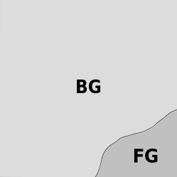
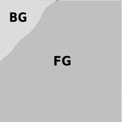
Block A

Block B

Figure 1: Without taking into account block overlapping, misclassification is inevitable at the pixel level whenever a given block has both foreground (FG) and background (BG) pixels. Classifying Block A as background results in a few false negatives (foreground pixels classified as background) while classifying Block B as foreground results in a few false positives (background pixels classified as foreground).

III Experiments

In this section, we first provide a brief description of the datasets used in our experiments in Section III-A. We then evaluate the effect of two key parameters (block size and block advancement) and the contribution of the three classifier stages to overall performance in Sections III-B and III-C, respectively.

For comparative evaluation, we conducted two sets of experiments: (i) subjective and objective evaluation of foreground segmentation efficacy, using datasets with available ground-truths; (ii) comparison of the effect of the various foreground segmentation methods on tracking performance. The details of the experiments are described in Sections III-D and III-E, respectively.

The proposed algorithm was implemented in C++ with the aid of Armadillo [56] and OpenCV libraries [57]. All experiments were conducted on a standard 3 GHz machine.

III-A Datasets

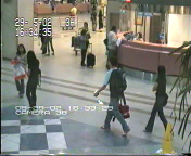
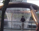
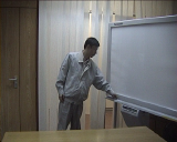
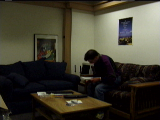
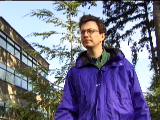
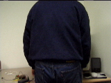
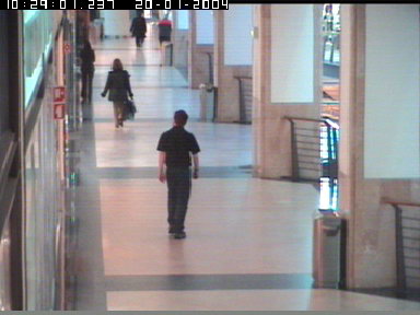
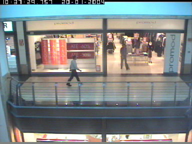
We use three datasets for the experiments: I2R, Wallflower, and CAVIAR. The I2R dataset has nine sequences captured in diverse and challenging environments characterised by complex backgrounds such as waving trees, fountains, and escalators. Furthermore, the dataset also exhibits the phenomena of illumination variations and cast shadows. For each sequence there are 20 randomly selected images for which the ground-truth foreground masks are available. The Wallflower dataset has seven sequences, with each sequence being a representative of a distinct problem encountered in background modelling [55]. The background is subjected to various phenomena which include sudden and gradual lighting changes, dynamic motion, camouflage, foreground aperture, bootstrapping and movement of background objects within the scene. Each sequence has only one ground-truth foreground mask. The second subset of CAVIAR, used for the tracking experiments, has 52 sequences with tracking ground truth data (ie. object positions). Example images from the three datasets are given in Figures 8, 9 and 10.

III-B Effects of Block Size and Advancement (Overlapping)

In this section we evaluate the effect of block size and block advancement to the overall performance. For quantitative evaluation we adopted the F-measure metric used by Brutzer et al. [12], which quantifies how similar the obtained foreground mask is to the ground-truth:

$$\operatorname{\it F-measure}=2\frac{recall\cdot precision}{recall+precision}$$ (7)

where $\operatorname{\it F-measure}$ $\in[0,1]$, while $precision$ and $recall$ are given by $\frac{tp}{tp+fp}$ and $\frac{tp}{tp+fn}$, respectively. The notations $tp$, $fp$ and $fn$ are total number of true positives, false positives and false negatives (in terms of pixels), respectively. The higher the $\operatorname{\it F-measure}$ value, the more accurate the foreground segmentation.

TABLE I: Accuracy of foreground estimation for various block sizes on the I2R and Wallflower datasets, with the block advancement fixed at 1 (ie. maximum overlap). Accuracy was measured by $\operatorname{\it F-measure}$ averaged over all frames where ground-truth is available. The ‘mean’ column indicates the mean of the values obtained for the two datasets.

Block Size	Average $\operatorname{\it F-measure}$
	I2R	Wallflower	mean
2$\times$2	0.726	0.588	0.657
4$\times$4	0.791	0.633	0.712
6$\times$6	0.790	0.714	0.752
8$\times$8	0.780	0.733	0.756
10$\times$10	0.760	0.735	0.735
12$\times$12	0.732	0.729	0.731
14$\times$14	0.704	0.715	0.710
16$\times$16	0.659	0.692	0.675

Table I shows the performance of the proposed algorithm for block sizes ranging from 2$\times$2 to 16$\times$16, with the block advancement fixed at 1 (ie. maximum overlap between blocks). The optimal block size for the I2R dataset is 4$\times$4, with the performance being quite stable from 4$\times$4 to 8$\times$8. For the Wallflower dataset the optimal size is 10$\times$10, with similar performance obtained using 8$\times$8 to 12$\times$12. By taking the mean of the values obtained for each block size across both datasets, the overall optimal size appears to be 8$\times$8. This block size is used in all following experiments.

(a)

(b)

(c)

(d)

(e)

(f)

Figure 2: (a) An example frame from the I2R dataset, (b) its corresponding ground-truth foreground mask. Using the proposed method with a block size of $8\times 8$, the foreground masks obtained for various degrees of block advancement: (c) 1 pixel, (d) 2 pixels, (e) 4 pixels, and (f) 8 pixels (ie. no overlap).

(a)

(b)

Figure 3: Effect of block advancements on: (a) $\operatorname{\it F-measure}$ value and (b) processing speed in terms of frames per second obtained using the I2R dataset. A considerable gain in processing speed is achieved as the advancement between blocks increases, at the expense of a gradual decrease in $\operatorname{\it F-measure}$ values.

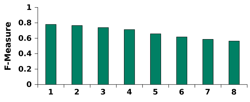
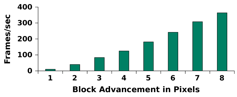
Figures 2 and 3 show the effect of block advancement on foreground segmentation accuracy and processing speed on the I2R dataset. As the block size is fixed to 8$\times$8, block advancement of 8 pixels (between successive blocks) indicates no overlapping, while block advancement of 1 pixel denotes maximum overlap. The smaller the block advancement (ie. higher overlap), the higher the accuracy and smoother object contours, at the expense of a considerable increase in the computational load (due to more blocks that need to be processed). A block advancement of 1 pixel achieves the best $\operatorname{\it F-measure}$ value of 0.78, at the cost of low processing speed (10 frames per second). Increasing the block advancement to 2 pixels somewhat decreases the $\operatorname{\it F-measure}$ value to 0.76, but the processing speed raises to 40 frames per second.

(a)

(b)

 

(c)

(d)

(e)

Figure 4: (a) Example frames from I2R dataset. (b) Ground truth foreground masks. Foreground masks obtained by the proposed method using: (c) the first classifier only, (d) combination of the first and second classifiers, (e) using all three classifiers. Adding the second classifier considerably improves the segmentation quality, while the addition of the third classifier aids in minor reduction of false positives. See Fig. 5 for quantitative results.

Figure 5: Impact of individual classifiers on the overall segmentation quality for various block advancement values, using the I2R dataset. The best results are achieved when all 3 classifiers are used (default configuration).

III-C Contribution of Individual Classifier Stages

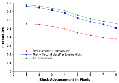
In the proposed algorithm, each classifier (see Section II-B) handles a distinct problem such as dynamic backgrounds and varying illuminations. In this section, the influence of individual classifiers to the overall segmentation performance is further investigated. We evaluate the segmentation quality using three separate configurations: (i) classification using the first classifier (based on multivariate Gaussian density function) alone, (ii) classification using a combination of the first classifier followed by the second (based on cosine distance), (iii) classification using all stages. The the qualitative results of each configuration using the I2R dataset are shown in Fig. 4. The quantitative results of each configuration for various block advancements are shown in Fig. 5.

We note that the best segmentation results are obtained for the default configuration when all 3 classifiers are used. The next best configuration is the combination of the first and second classifiers which independently inspect for scene changes occurring due to dynamic backgrounds and illumination variations, respectively. The configuration comprising of only the first classifier yields the lowest $\operatorname{\it F-measure}$ value, since background variations due to illumination are not handled effectively by it.

We note the impact of the third classifier appears to be minor compared to that of the second, since it is aimed to minimise the occasional false positives by examining the temporal correlations between consecutive frames (see Section II-B(c)). The relative improvement in average $\operatorname{\it F-measure}$ value achieved by adding the second classifier is about 37%, while adding the third gives further relative improvement of about 5%. Qualitative results of each configuration shown in Figure 4 confirm the above observations.

Figure 6: Comparison of $\operatorname{\it F-measure}$ values (defined in Eqn. (7)) obtained on the I2R dataset using foreground segmentation methods based on GMMs [23], feature histograms [27], NVD [42], SOM [39], SA [37] and the proposed method. The higher the $\operatorname{\it F-measure}$ (ie. agreement with ground-truth), the better the segmentation result.

Figure 7: As per Fig. 6, but obtained on the Wallflower dataset. Due to the absence of true positives in the ground-truth for the moved object sequence, the corresponding F-measure is zero for all algorithms.

III-D Comparative Evaluation by Ground-Truth F-measure

The proposed algorithm is compared with segmentation methods based on Gaussian mixture models (GMMs) [23], feature histograms [27], probabilistic self organising maps (SOM) [39], stochastic approximation (SA) [37] and normalised vector distances (NVD) [42]. The first four methods classify individual pixels into foreground or background, while the last method makes decisions on groups of pixels.

We used the OpenCV v2.0 [57] implementations for the GMM and feature histogram based methods with default parameters, except for setting the learning parameter in GMM to 0.001. Experiments showed that the above parameter settings produce optimal segmentation performance. We used the implementations made available by the authors’ for SOM and SA methods.

Post-processing using morphological operations was required for the foreground masks obtained by the GMM, feature histogram and SOM methods, in order to clean up the scattered error pixels. For the GMM method, opening followed by closing using a $3\times 3$ kernel was performed, while for the feature histogram method we enabled the built-in post-processor (using default parameters suggested in the OpenCV implementation). We note that the proposed method does not require any such ad-hoc post-processing.

With the view of designing a pragmatic system, the same parameter settings were used across all sequences (ie. they were not optimised for any particular sequence). Specifically, during deployment a practical system has to perform robustly in many scenarios.

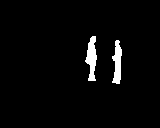
We present both qualitative and quantitative analysis of the results. Figs. 6 and 7 show quantitative results for the I2R and Wallflower datasets, respectively. The corresponding qualitative results for three sequences from each dataset are shown in Figs. 8 and 9.

(a)

(b)

 

(c)

(d)

(e)

(f)

(g)

(h)

Figure 8: (a) Example frames from three video sequences in the I2R dataset. Left: people walking at an airport, with significant cast shadows. Middle: people moving against a background of a fountain with varying illumination. Right: a person walks in and out of a room where the window blinds are non-stationary, with illumination variations caused by automatic gain control of the camera. (b) Ground-truth foreground mask, and foreground mask estimation using: (c) GMM based [23] with morphological post-processing,  (d) feature histograms [27], (e) NVD [42],  (f) SOM [39], (g) SA [37], (h) proposed method.

(a)

(b)

 

(c)

(d)

(e)

(f)

(g)

(h)

Figure 9: As per Fig. 8, but using the Wallflower dataset. Left: room illumination gradually increases over time and a person walks in and sits on the couch. Middle: person walking against a background of strongly waving trees and the sky. Right: a monitor displaying a blue screen with rolling bars is occluded by a person wearing blue coloured clothing.

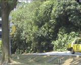
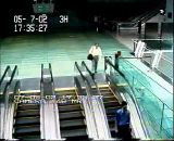
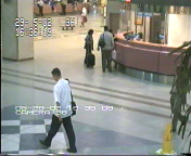
In Fig. 8, the AP sequence (left column) has significant cast shadows of people moving at an airport. The FT sequence (middle column) contains people moving against a background of a fountain with varying illumination. The MR sequence (right column) shows a person entering and leaving a room where the window blinds are non-stationary and there are significant illumination variations caused by the automatic gain control of the camera.

In Fig. 9, the time of day sequence (left column) has a gradual increase in the room’s illumination intensity over time. A person walks in and sits on the couch. The waving trees sequence (middle column) has a person walking against a background consisting of the sky and strongly waving trees. In the camouflage sequence (right column), a monitor has a blue screen with rolling bars. A person in blue coloured clothing walks in and occludes the monitor.

We note that output of the GMM based method (column c in Figs. 8 and 9) is sensitive to reflections, illumination changes and cast shadows. While the histogram based method (column d) overcomes these limitations, it has a lot of false negatives. The NVD based method (column e) is largely robust to illumination changes, but fails to handle dynamic backgrounds and produces ‘blocky’ foreground masks. The SOM and SA based methods have relatively few false positives and negatives. The results obtained by the proposed method (column f) are qualitatively better than those obtained by the other five methods, having low false positives and false negatives. However, we note that due to the the block-based nature of the analysis, objects very close to each other tend to merge.

The quantitative results (using the F-measure metric) obtained on the I2R and Wallflower datasets, shown in Figs. 6 and 7, respectively, largely confirm the visual results. On the I2R dataset the proposed method outperforms the other methods in most cases. The next best method (SOM) obtained an average $\operatorname{\it F-measure}$ value of 0.72, while the proposed method achieved 0.78, representing an improvement of about 8%.

On the Wallflower dataset the proposed method achieved considerably better results for the foreground aperture sequence. While for the remainder of the sequences the performance was roughly on par with the other methods, the proposed method nevertheless still achieved the highest average $\operatorname{\it F-measure}$ value. The next best method (histogram of features) obtained an average value of 0.66, while the proposed method obtained 0.73, representing an improvement of about 11%.

We note that the performance of the proposed method on Bootstrapping sequence is lower. We conjecture that this is due to foreground objects occluding background during the training phase. Robust background initialisation techniques [50, 51] capable of estimating the background in cluttered sequences could be used to alleviate this problem.

III-E Comparative Evaluation by Tracking Precision & Accuracy

We conducted a second set of experiments to evaluate the performance of the segmentation methods in more pragmatic terms rather than limiting ourselves to the traditional ground-truth evaluation approach. To this effect, we evaluated the influence of the various foreground detection algorithms on tracking performance. The foreground masks obtained from the detectors for each frame of the sequence were passed as input to an object tracking system. We have used a particle filter based tracker as implemented in the video surveillance module of OpenCV v2.0 [57]. Here the foreground masks are used prior to tracking for initialisation purposes.

Tracking performance was measured with the two metrics proposed by Bernardin and Stiefelhagen [58], namely multiple object tracking precision (MOTP) and multiple object tracking accuracy (MOTA).

Briefly, MOTP measures the average pixel distance between ground-truth locations of objects and their locations according to a tracking algorithm. Ground truth objects and hypotheses are matched using Munkres’ algorithm [59]. MOTP is defined as:

$$\operatorname{MOTP}={\sum\nolimits_{i,t}d_{t}^{i}}~{}/~{}{\sum\nolimits_{t}c_{t}}$$ (8)

where $d_{t}^{i}$ is the distance between object $i$ and its corresponding hypothesis, while $c_{t}$ is the number of matches found at time $t$. The lower the MOTP, the better.

MOTA accounts for object configuration errors, false positives, misses as well as mismatches. It is defined as:

$$\operatorname{MOTA}=1-\frac{{\sum_{t}(m_{t}+fp_{t}+mme_{t})}}{\sum_{t}g_{t}}$$ (9)

It measures accuracy in terms of the number of false negatives ($m$), false positives ($fp$) and mismatch errors ($mme$) with respect to the number of ground truth objects ($g$). The higher the value, the better the accuracy. The MOTA value can become negative in certain circumstances when the false negatives, false positives and mismatch errors are considerably large, making the ratio in Eqn. (9) greater than unity [58].

Figure 10: Example frames from the second subset of the CAVIAR dataset, used for evaluating the influence of various foreground detection algorithms on tracking performance.

TABLE II: Effect of various settings of block advancement on multiple object tracking accuracy (MOTA) in terms of percentage, and multiple object tracking precision (MOTP) in terms of pixels. Results are obtained on second subset of CAVIAR by using a particle-filter based tracking algorithm.

Block Advancement	Tracking Metrics
	MOTA	MOTP
	(higher is better)	(lower is better)
1	30.3	11.7
2	20.4	11.8
4	8.6	12.4
8	$-$67.3	14.7

TABLE III: As per Table. II, but obtained by employing various foreground detection methods.

Foreground detection	Tracking Metrics
	MOTA	MOTP
	(higher is better)	(lower is better)
GMM based method [23]	27.2	13.6
NVD based method [42]	$-$24.9	15.2
Histogram of features [27]	13.7	14.7
SOM [39]	26	13.3
SA [37]	27.3	13.0
Proposed method	30.3	11.7

The performance result is the average performance of the 52 test sequences belonging to the second subset of CAVIAR. To keep the evaluations more realistic, the first few frames (200 frames) of each sequence are used to train the background model irrespective of the presence of foreground objects (ie. background frames were not handpicked for training).

We first evaluated the tracking performance for various block advancements. Results presented in Table II indicate that a block advancement of 1 pixel obtains the best tracking performance, while larger advancements lead to a decrease in performance.

Comparisons with GMM, histogram of features and NVD, presented in Table III, indicate that the proposed method leads to considerably better tracking performance. For tracking accuracy (MOTA), the next best method (SA) led to an average accuracy of 27.3%, while the proposed method led to 30%. For tracking precision (MOTP), the next best method (SA) led to an average pixel distance of 13, while the proposed method reduced the distance to 11.7.

IV Main Findings

Pixel-based processing approaches to foreground detection can be susceptible to noise, illumination variations and dynamic backgrounds, partly due to not taking into account rich contextual information. In contrast, region-based approaches mitigate the effect of above phenomena but suffer from ‘blockiness’ artefacts. The proposed foreground detection method belongs to region-based category, but at the same time is able segment smooth contours of foreground objects.

Contextual spatial information is employed through analysing each frame on an overlapping block-by-block basis. The low-dimensional texture descriptor for each block alleviates the effect of image noise. The model initialisation strategy allows the training sequence to contain moving foreground objects. The adaptive classifier cascade analyses the descriptor from various perspectives before classifying the corresponding block as foreground. Specifically, it checks if disparities are due to background motion or illumination variations, followed by a temporal correlation check to minimise the occasional false positives emanating due to background characteristics which were not handled by the preceding classifiers.

The probabilistic foreground mask generation approach integrates the block-level classification decisions by exploiting the overlapping nature of the analysis, ensuring smooth contours of the foreground objects as well as effectively minimising the number of errors. Unlike many pixel-based methods, ad-hoc post-processing of foreground masks is not required.

Experiments conducted to evaluate the standalone performance (using the difficult Wallflower and I2R datasets) show the proposed method obtains on average better results (both qualitatively and quantitatively) than methods based on GMMs, feature histograms, normalised vector distances, self organising maps and stochastic approximation.

We furthermore proposed the use of tracking performance as an unbiased approach for assessing the practical usefulness of foreground segmentation methods, and demonstrated that the proposed method leads to considerable improvements in object tracking accuracy on the CAVIAR dataset.

References

- [1] F. Porikli and O. Tuzel. Human body tracking by adaptive background models and mean-shift analysis. IEEE International Workshop on Performance Evaluation of Tracking and Surveillance, 2003.
- [2] O. Javed and M. Shah. Tracking and object classification for automated surveillance. Lecture Notes in Computer Science, vol. 2353, 2006, pp. 439–443.
- [3] F. Lv and R. Nevatia. Single view human action recognition using key pose matching and Viterbi path searching. IEEE Conference on Computer Vision and Pattern Recognition, 2007, pp. 1–8.
- [4] L. Wang, T. Tan, H. Ning, and W. Hu. Silhouette analysis-based gait recognition for human identification. IEEE Transactions on Pattern Analysis and Machine Intelligence, vol. 25, no. 12, pp. 1505–1518, 2003.
- [5] T. Xiang and S. Gong. Incremental and adaptive abnormal behaviour detection. Computer Vision and Image Understanding, vol. 111, no. 1, pp. 59–73, 2008.
- [6] V. Reddy, C. Sanderson, and B. Lovell. Improved anomaly detection in crowded scenes via cell-based analysis of foreground speed, size and texture. IEEE Conference on Computer Vision and Pattern Recognition Workshops, 2011, pp. 55–61.
- [7] A. Criminisi, G. Cross, A. Blake, and V. Kolmogorov. Bilayer segmentation of live video. IEEE Conference on Computer Vision and Pattern Recognition, vol. 1, 2006, pp. 53–60.
- [8] J. Vass, K. Palaniappan, and X. Zhuang. Automatic spatio-temporal video sequence segmentation. IEEE International Conference on Image Processing, vol. 1, 1998, pp. 958–962.
- [9] A. Neri, S. Colonnese, G. Russo, and P. Talone. Automatic moving object and background separation. Signal Processing, vol. 66, no. 2, pp. 219–232, 1998.
- [10] A. Agarwala, M. Dontcheva, M. Agrawala, S. Drucker, A. Colburn, B. Curless, D. Salesin, and M. Cohen. Interactive digital photomontage. ACM Transactions on Graphics, vol. 23, pp. 294–302, 2004.
- [11] M. Piccardi. Background subtraction techniques: a review. Proceedings of the IEEE International Conference on Systems, Man and Cybernetics, vol. 4, 2004, pp. 3099–3104.
- [12] S. Brutzer, B. Höferlin, and G. Heidemann. Evaluation of background subtraction techniques for video surveillance. IEEE Conference on Computer Vision and Pattern Recognition, 2011, pp. 1937–1944.
- [13] T. Bouwmans, F. El Baf, and B. Vachon. Background modeling using mixture of Gaussian for foreground detection - a survey. Recent Patents on Computer Science, vol. 1, no. 3, pp. 219–237, 2008.
- [14] T. Bouwmans, F. El Baf, and B. Vachon. Statistical background modeling for foreground detection: A survey. Handbook of Pattern Recognition and Computer Vision. World Scientific Publishing, 2010, vol. 4, ch. 2.3, pp. 181–199.
- [15] J. Barron, D. Fleet, and S. Beauchemin. Performance of optical flow techniques. International Journal of Computer Vision, vol. 12, no. 1, pp. 43–77, 1994.
- [16] P. Kohli and P. Torr. Dynamic graph cuts for efficient inference in Markov random fields. IEEE Transactions on Pattern Analysis and Machine Intelligence, vol. 29, no. 12, pp. 2079–2088, 2007.
- [17] P. Viola and M. Jones Robust real-time face detection. International Journal of Computer Vision, vol. 57, no. 2, pp. 137–154, 2004.
- [18] N. Dalal and B. Triggs. Histograms of oriented gradients for human detection. IEEE Conference on Computer Vision and Pattern Recognition, vol. 1, 2005, pp. 886–893.
- [19] E. Trucco and A. Verri. Introductory Techniques for 3-D Computer Vision. Prentice Hall, 1998.
- [20] V. Reddy, C. Sanderson, A. Sanin, and B. Lovell. Adaptive patch-based background modelling for improved foreground object segmentation and tracking. International Conference on Advanced Video and Signal Based Surveillance, 2010, pp. 172–179.
- [21] M. Cristani, M. Farenzena, D. Bloisi, and V. Murino. Background subtraction for automated multisensor surveillance: a comprehensive review. EURASIP Journal on Advances in Signal Processing, vol. 2010, pp. 1–24, 2010.
- [22] C. Stauffer and W. Grimson. Adaptive background mixture models for real-time tracking. IEEE Conference on Computer Vision and Pattern Recognition, vol. 2, 1999, pp. 246–252.
- [23] P. KaewTraKulPong and R. Bowden. An improved adaptive background mixture model for real-time tracking with shadow detection. Proceedings of the 2nd European Workshop Advanced Video Based Surveillance Systems, vol. 1, 2001, pp. 1–5.
- [24] Z. Zivkovic. Improved adaptive Gaussian mixture model for background subtraction. International Conference on Pattern Recognition, vol. 2, 2004, pp. 28–31.
- [25] L. Teixeira, J. Cardoso, and L. Corte-Real. Object segmentation using background modelling and cascaded change detection. Journal of Multimedia, vol. 2, no. 5, pp. 55–65, 2007.
- [26] A. Elgammal, D. Harwood, and L. Davis. Non-parametric model for background subtraction. Lecture Notes in Computer Science, vol. 1843, 2000, pp. 751–767.
- [27] L. Li, W. Huang, I. Gu, and Q. Tian. Foreground object detection from videos containing complex background. ACM International Conference on Multimedia, 2003, pp. 2–10.
- [28] B. Han and L. Davis. Density-based multifeature background subtraction with support vector machine. IEEE Transactions on Pattern Analysis and Machine Intelligence, vol. 34, no. 5, pp. 1017–1023, 2012.
- [29] T. Parag, A. Elgammal, and A. Mittal. A framework for feature selection for background subtraction. IEEE Conference on Computer Vision and Pattern Recognition, vol. 2, 2006, pp. 1916–1923.
- [30] L. Cheng, M. Gong, D. Schuurmans, and T. Caelli. Real-time discriminative background subtraction. IEEE Transactions on Image Processing, vol. 20, no. 5, pp. 1401–1414, 2011.
- [31] A. Shimada and R. Taniguchi. Hybrid background model using spatial-temporal LBP. IEEE International Conference on Advanced Video and Signal Based Surveillance, 2009, pp. 19–24.
- [32] T. Tanaka, A. Shimada, D. Arita, and R.-i. Taniguchi. Object detection under varying illumination based on adaptive background modeling considering spatial locality. Lecture Notes in Computer Science, vol. 5414, 2009, pp. 645–656.
- [33] J.-M. Guo, Y.-F. Liu, C.-H. Hsia, M.-H. Shih, and C.-S. Hsu. Hierarchical method for foreground detection using codebook model. IEEE Transactions on Circuits and Systems for Video Technology, vol. 21, no. 6, pp. 804–815, 2011.
- [34] O. Javed and M. Shah. Automated Multi-Camera Surveillance: Algorithms and Practice. Springer, 2008.
- [35] N. Oliver, B. Rosario, and A. Pentland. A Bayesian computer vision system for modeling human interactions. IEEE Transactions on Pattern Analysis and Machine Intelligence, vol. 22, no. 8, pp. 831–843, 2000.
- [36] L. Wang, L. Wang, M. Wen, Q. Zhuo, and W. Wang. Background subtraction using incremental subspace learning. IEEE International Conference on Image Processing, vol. 5, 2007, pp. 45–48.
- [37] E. López-Rubio and R. M. L. Baena. Stochastic approximation for background modelling. Computer Vision and Image Understanding, vol. 115, no. 6, pp. 735–749, 2011.
- [38] L. Maddalena and A. Petrosino. A self-organizing approach to background subtraction for visual surveillance applications. IEEE Transactions on Image Processing, vol. 17, no. 7, pp. 1168–1177, 2008.
- [39] E. López-Rubio, R. M. L. Baena, and E. Domínguez. Foreground detection in video sequences with probabilistic self-organizing maps. International Journal of Neural Systems, vol. 21, no. 3, pp. 225–246, 2011.
- [40] R. Gonzalez and R. Woods. Digital Image Processing, 3rd edition. Pearson Prentice Hall, 2007.
- [41] M. Mason and Z. Duric. Using histograms to detect and track objects in color video. Applied Imagery Pattern Recognition Workshop, 2001, pp. 154–159.
- [42] T. Matsuyama, T. Wada, H. Habe, and K. Tanahashi. Background subtraction under varying illumination. Systems and Computers in Japan, vol. 37, no. 4, pp. 77–88, 2006.
- [43] H. Grabner, C. Leistner, and H. Bischof. Time dependent on-line boosting for robust background modeling. Computer Vision Theory and Applications, 2008, pp. 612–618.
- [44] Y. Lee, J. Jung, and I. Kweon. Hierarchical on-line boosting based background subtraction. Workshop on Frontiers of Computer Vision, 2011, pp. 1–5.
- [45] M. Seki, T. Wada, H. Fujiwara, and K. Sumi. Background subtraction based on cooccurrence of image variations. IEEE Conference on Computer Vision and Pattern Recognition, vol. 2, 2003, pp. 65–72.
- [46] A. Chan and N. Vasconcelos. Modeling, clustering, and segmenting video with mixtures of dynamic textures. IEEE Transactions on Pattern Analysis and Machine Intelligence, vol. 30, no. 5, pp. 909–926, 2008.
- [47] D. Pokrajac and L. Latecki. Spatiotemporal blocks-based moving objects identification and tracking. IEEE Visual Surveillance and Performance Evaluation of Tracking and Surveillance, 2003, pp. 70–77.
- [48] A. Sanin, C. Sanderson, and B. Lovell. Shadow detection: A survey and comparative evaluation of recent methods. Pattern Recognition, vol. 45, no. 4, pp. 1684–1695, 2012.
- [49] C. Sanderson and B. Lovell. Multi-region probabilistic histograms for robust and scalable identity inference. Lecture Notes in Computer Science, vol. 5558, 2009, pp. 199–208.
- [50] D. Baltieri, R. Vezzani, and R. Cucchiara. Fast background initialization with recursive Hadamard transform. International Conference on Advanced Video and Signal Based Surveillance, 2010, pp. 165–171.
- [51] V. Reddy, C. Sanderson, and B. Lovell. A low complexity algorithm for static background estimation from cluttered image sequences in surveillance contexts. EURASIP Journal on Image and Video Processing, vol. 2011, pp. 1–14, 2011.
- [52] R. Duda, P. Hart, and D. Stork. Pattern Classification, 2nd edition. John Wiley & Sons, New York, USA, 2001.
- [53] C. Wren, A. Azarbayejani, T. Darrell, and A. Pentland. Pfinder: Real-time tracking of the human body. IEEE Transactions on Pattern Analysis and Machine Intelligence, vol. 19, no. 7, pp. 780–785, 1997.
- [54] K. Kim, T. Chalidabhongse, D. Harwood, and L. Davis. Real-time foreground–background segmentation using codebook model. Real-Time Imaging, vol. 11, no. 3, pp. 172–185, 2005.
- [55] K. Toyama, J. Krumm, B. Brumitt, and B. Meyers. Wallflower: Principles and practice of background maintenance. IEEE International Conference on Computer Vision, vol. 1, 1999, pp. 255–261.
- [56] C. Sanderson. Armadillo: An open source C++ linear algebra library for fast prototyping and computationally intensive experiments. Technical Report, NICTA, 2010.
- [57] G. Bradski and A. Kaehler. Learning OpenCV: Computer Vision with the OpenCV Library. O’Reilly Media, 2008.
- [58] K. Bernardin and R. Stiefelhagen. Evaluating multiple object tracking performance: the CLEAR MOT metrics. EURASIP Journal on Image Video Processing, vol. 2008, pp. 1–10, 2008.
- [59] J. Munkres. Algorithms for the assignment and transportation problems. Journal of the Society for Industrial and Applied Mathematics, vol. 5, no. 1, pp. 32–38, 1957.