PHOTOMETRIC REDSHIFTS AND SYSTEMATIC VARIATIONS IN THE SPECTRAL ENERGY DISTRIBUTIONS OF LUMINOUS RED GALAXIES FROM THE SDSS DR7
Abstract
We describe the construction of a template set of spectral energy distributions (SEDs) for the estimation of photometric redshifts of luminous red galaxies (LRGs) with a Bayesian template fitting method. By examining the color properties of several publicly available SED sets within a redshift range of and comparing them to Sloan Digital Sky Survey (SDSS) Data Release 7 data, we show that only some of the investigated SEDs approximately match the colors of the LRG data throughout the redshift range, however not at the quantitative level required for precise photometric redshifts. This is because the SEDs of galaxies evolve with time (and redshift) and because at fixed redshift the LRG colors have an intrinsic spread such that they cannot be matched by one SED only. We generate new SEDs by superposing model SEDs of composite stellar populations with a burst model, allowing both components to be reddened by dust, in order to match the data in five different redshift bins. We select a set of SEDs which represents the LRG data in color space within five redshift bins, thus defining our new SED template set for photometric redshift estimates. The results we get with the new template set and our Bayesian template fitting photometric redshift code (PhotoZ) are nearly unbiased, with a scatter of (including outliers), a fraction of catastrophic outliers () of , and a normalized median absolute rest frame deviation (NMAD) of for non-outliers. We show that templates that optimally describe the brightest galaxies () indeed vary from to , consistent with aging of the stellar population. Furthermore, we find that templates that optimally describe galaxies at strongly differ as a function of the absolute magnitude of the galaxies, indicating an increase in star formation activity for less luminous galaxies. Our findings based on the photometry of the SDSS LRGs and our SED template fitting are supported by comparison to the average SDSS LRG spectra in different luminosity and redshift bins.
Subject headings:
galaxies: distances and redshifts – galaxies: evolution – galaxies: fundamental parameters (colors)1. Introduction
The primary goal of our work is to generate new spectral energy distributions (SEDs) for luminous red galaxies (LRGs) to obtain precise photometric redshift measurements from template fitting methods.
For the analysis of large scale structure (LSS) based on photometric redshift distances it is important to precisely know the photometric redshift errors and biases and to make these as small as possible.
For dark energy constraints based on shear tomography it is most important to know the errors and biases precisely (Ma et al., 2006), but on the other hand the rms-size of the photometric redshift errors determines how many tomographic redshift bins can be analyzed for a given survey.
In addition, if the bias changes strongly as a function of the (true) redshift, then it cannot be treated as being constant within a given tomographic interval anymore, which makes the analysis of such data more difficult.
Another reason why small photometric redshift uncertainties are advantageous is the following.
When the baryonic acoustic oscillation (BAO) scale is extracted from galaxy clustering measurements obtained with distances based on photometric redshifts (see Sánchez et al. 2011, and Benítez et al. 2009 for the case of the transversal BAO scale, and Roig et al. 2009 for the case of the radial direction), the quality of the result dramatically depends on the photometric redshift errors (see Figure 3 of Benítez et al. 2009, and Figure 1 of Sánchez et al. 2011).
When galaxy properties (colors, star formation rate, dark matter halo properties) are studied as a function of their environment density based on photometric redshift distances (see, e.g., Capak et al. 2007 and Chuter et al. 2011 for an example), redshift errors introduce biases in density, because galaxies are being preferentially scattered out of high density environments into the low density environments.
In these cases it is also very important to have a low SED dependence of bias, or to at least know the bias very well as a function of SED and redshift.
Finally, redshift errors imply large errors of the estimated absolute luminosities and stellar masses (see Nakajima et al. 2012, Figure 13).
If one then studies average galaxy properties as a function of absolute luminosity or stellar mass, one has to account for contamination from galaxies originating from other luminosity bins.
In summary, it is important to know bias and redshift scatter, but it is also important to aim for a scatter that is as small as possible, since any scatter corresponds to a loss of information.
We will generate new template SEDs which optimally reproduce the LRG colors by fitting composite stellar populations (CSPs) and an extincted starburst component to the broadband photometric Sloan Digital Sky Survey (SDSS) data.
We thus also obtain hints for the mechanism causing the observed changes, i.e., a luminosity and redshift dependence of star formation history (SFH).
Broadband photometry however is not the best method to study this, given that different ages and metallicities can produce fairly similar colors.
This degeneracy can only be rigorously broken with spectroscopic information.
We could use priors (i.e., exclude low metallicities) from the beginning, and then interpret the best fitting SEDs in terms of SFH.
Instead, we want to make use of the full variety of different colors that can be generated even with implausible ingredients (i.e., age–metallicity combination, but also extinction which changes the slope of an SED) to increase the flexibility of SEDs that can be generated.
We will see in Section 7.1, however, that the broadband near-UV (NUV) and far-UV (FUV) colors of our newly generated SEDs match the sequence of colors of quiescent to star-forming early-type galaxies (ETGs) classified by spectroscopic analyses.
This means that generating SEDs by fitting galaxy colors with a composite population plus a burst population is not just a method to increase the freedom of SEDs in the - to -band (rest frame) wavelength ranges, but that it is very plausible that some of the LRGs do show signs of recent star formation.
In this paper we concentrate on the estimation of photometric redshifts (photo-s) for spectroscopically observed LRGs
from the SDSS Data Release 7 (York et al., 2000; Abazajian et al., 2009).
LRGs mostly consist of ETGs and show rather uniform SEDs (Schneider et al., 1983; Eisenstein et al., 2003).
Most importantly, their SEDs have a pronounced break at 4000 Å which is due to an accumulation of metal lines.
The 4000 Å break together with the spectral uniformity are the reasons why photometric redshift estimations are very precise for red galaxy types.
LRGs are also of great cosmological interest: They are among the most luminous galaxies existing, are strongly correlated with each other, since they are preferentially located in dense regions of the universe, they closely map its LSS.
This paper is organized as follows: In Section 2 we briefly present the photometric redshift code used in this paper.
After that we will shortly explain the data set and investigate the differences between the colors of the data and specific model SEDs (Section 3).
In Section 4 we present the method with which we generate new SEDs based on the LRG photometry.
The photometric redshift results using the new template SEDs are analyzed in Section 5 and compared to public SDSS photo-s in Section 6.
A discussion about the properties of the new SEDs is given in Section 7, where we investigate the FUV and NUV colors in Section 7.1 and show systematic variations in the SEDs in Section 7.2.
We show the results of SED fitting different model sets to the LRG photometry in Appendix A.
The colors of the created model SEDs will be investigated in greater detail in Appendix B.
Throughout this paper we assume a cosmology with , and , while magnitudes are given in the AB system.
2. Photometric Redshifts with Template Fitting Methods and the PhotoZ Code
The techniques to estimate photometric redshifts can be divided into two main categories: empirical and template fitting methods. The former use a training set of galaxies with known spectroscopic redshifts and photometry to derive an empirical relation between the redshift and the photometric observables. The latter fit template SEDs to the photometry of objects, thereby determining the most probable redshift (Arnouts et al., 1999; Benítez, 2000; Bolzonella et al., 2000; Csabai et al., 2000; Bender et al., 2001; Le Borgne & Rocca-Volmerange, 2002; Babbedge et al., 2004; Feldmann et al., 2006; Brammer et al., 2008). The simplest approach is to perform solely a minimization of the difference between the expected colors of a SED template and observed photometry, whereas hybrid photometric redshift methods combine a maximum likelihood approach together with an optimization routine to enhance the initial template set (e.g., by using a spectroscopic training set). Bayesian methods, on the other hand, use minimization, but additionally provide the opportunity to introduce redshift and luminosity priors which assign probability functions to the templates, thus enabling one to lift possible degeneracies where models are equally probable at different redshifts. The model SEDs for template matching methods can either be derived empirically (e.g., Coleman et al., 1980), from stellar population models (e.g., Bruzual & Charlot, 2003), or a combination of both. The advantage of template fitting is that it does not only provide photometric redshift estimates, but also rest frame properties of the best fit models such as the SED type and the absolute magnitude. Second, if good SEDs are available, they can be used with any data set (independent of its photometric depth, or the filter system). Since several SED types and redshifts can match the colors of an observed object equally well, it is very important to optimize the redshift and the luminosity priors for each type, depending on the filter set and the data, i.e., photometric depth and galaxy properties (which, in turn, depend on the galaxy selection function).
2.1. The PhotoZ Code
In this work we use the Bayesian template fitting photometric redshift code PhotoZ (Bender et al., 2001). The calculation of the probabilities of the model-redshift combinations is based on Bayes’ theorem:
where and denote the colors and magnitudes of the photometric data, and are the model parameters and . is the likelihood function which is proportional to . The second factor is the prior distribution , with the probability functions of absolute magnitude and redshift for a template . These priors are specified a priori and enable us to assign specific probability distributions in redshift and absolute magnitude for every SED template. Both are parameterized as proportional to , where is the most probable value of , or . The priors were chosen in this functional form to be able to vary the transitions between regions of different probabilities in such a way that they may be both smooth and have a box-like shape. In this formula the integer controls the steepness of the probability decrease left and right of : The larger , the steeper the decrease (odd values make no sense, of course, as the integral over the probability would diverge). We set the prior to have a Gaussian shape (), in order to have a shallow transition from high to low probabilities. We will make particular use of the prior later on when using SEDs specifically designed for different redshift ranges. For the luminosity prior we set , , and , as luminosities are very rare among LRGs (see also Section 7.2, Figure 13) and are thereby excluded. Within this interval however, the luminosity probabilities are virtually equally distributed. Although the LRG sample contains only objects with , the allowed photometric redshift range for all PhotoZ runs is . In this way we can assure that the photometric redshift results truly are below , although a larger redshift range is allowed. This is important for future work with deeper surveys where the redshift range is not known a priori. The PhotoZ code has been extensively tested and was applied to a number of photometric catalogs (Drory et al., 2001; Gabasch et al., 2004; Feulner et al., 2005; Brimioulle et al., 2008; Gabasch et al., 2008; Brimioulle et al., 2013). It has also been successfully applied to the Pan-STARRS1 medium deep fields and is part of the PS1 Photometric Classification Server (Saglia et al., 2012).
3. The Data and Model SEDs
3.1. The LRG Sample
The data in this paper contains objects from the spectroscopic set of the SDSS Data Release 7 LRG sample (Eisenstein et al., 2001). The selection criteria for LRGs in SDSS separate them from the other galaxy types by cuts in color space, taking their evolution with redshift into account. Objects passing these criteria are flagged accordingly and can be obtained via the Catalog Archive Server111http://cas.sdss.org/astrodr7/en/ (CAS). SDSS LRGs are color-selected in such a way that their SEDs have prominent 4000 Å breaks. We remove objects from the SDSS spectroscopic LRG sample that do not pass the color cuts developed by Padmanabhan et al. (2005), which differ marginally from the selection criteria of Eisenstein et al. (2001). For a reasonable evaluation of the photometric redshift quality later on, we require that the spectroscopic redshift errors fulfill (the redshift resolution of the PhotoZ runs), and that the spectroscopic redshifts were determined with high confidence (). The studied LRG sample contains approximately objects. Unless mentioned otherwise, refer to the extinction corrected (Schlegel et al., 1998) model magnitudes of SDSS in the AB system (Oke & Gunn, 1983).
3.2. Colors of SED Templates versus Colors of SDSS LRGs
In order to obtain decent photometric redshift estimates with template fitting methods, the model-set has to represent the data well in all available colors. In this section we compare the color–redshift relations for several red SEDs with the observed SDSS LRG colors. The red SEDs are taken from model sets provided in commonly used template fitting photometric redshift codes. Additionally, we examine other SEDs from stellar population modeling such as those of Bruzual & Charlot (2003, hereafter BC03) and Maraston et al. (2009, hereafter M09).
3.2.1 The PhotoZ Standard Template Set
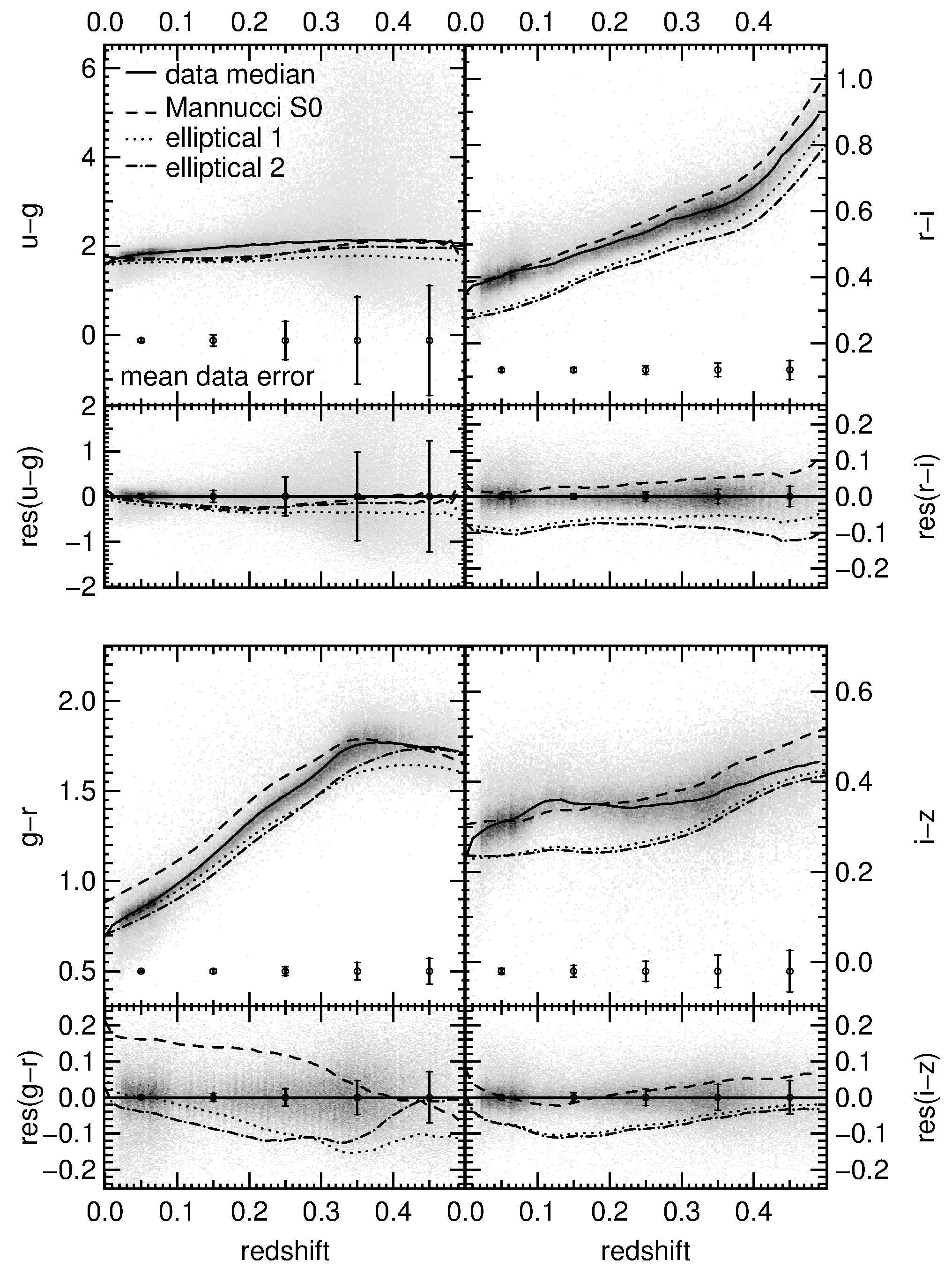
First, we investigate the three red template SEDs that have been used with the PhotoZ code until now (Gabasch et al., 2004; Feulner et al., 2005; Gabasch et al., 2008; Brimioulle et al., 2008). One of the models originates from Mannucci et al. (2001) and describes a galaxy with type S0. The other two SEDs were generated synthetically from single stellar populations of Bruzual & Charlot (1993) in order to describe two slightly different subsamples of red objects of the Hubble Deep Field (HDF) North at about to . The resulting two SEDs are rather similar, such that one of them could, in principle, be dropped in a photometric redshift analysis. In this case, however, photometric redshifts have shown to be less precise than for the case where both models have been used. For the success of photometric redshift estimates, it is relevant that the template SEDs cover, or at least span the whole color range. This is ensured by the Mannucci SED being too red and the other two SEDs being bluer regarding the 4000 Å break (i.e., the color for ; see Figure 1). Inspecting the SED colors in more detail (Figure 1) shows that, indeed, none of them describes the data equally well at all redshifts. Those created for the HDF are too blue in their colors for , and also in and throughout the whole range. The Mannucci S0 SED on the other hand is too red in at , and in at . It describes the observed color sufficiently well at . All three models match the data in within the errors, except for . The reason why these three SEDs give roughly correct redshifts for red galaxies is that the color has the strongest redshift sensitivity. Both ellipticals predict approximately correct values of for , whereas the Mannucci S0 matches the data well for . For that lie in between those ranges, red galaxies are either preferentially fitted by an elliptical or the Mannucci S0 SED, depending on the photometric errors and weights applied to the and data. For ground based data that are not as well calibrated as SDSS, the and band photometric errors are often scaled up to allow for an imprecisely known amount of telluric absorption. Furthermore, if an SED template color has an offset from the true color which is almost constant over the whole redshift range (as it is the case for of the two elliptical SEDs), then there is no contribution to a systematically wrong redshift estimate.
3.2.2 Models of Bruzual & Charlot 2003
The CSP models of Bruzual & Charlot (2003) can be generated with their software galaxev222http://www.cida.ve/~bruzual/bc2003 or http://www.iap.fr/~charlot/bc2003. We investigate SEDs from the (theoretical) BaSeL library with Padova 1994 evolutionary tracks and an initial mass function (IMF) of Chabrier (2003) and solar metallicity. The models have ages from to , and exponential star formation rates (SFRs) with -folding timescales between and (latter introduced to account for a constant SFR). Furthermore, we included a model that has no ongoing star formation and all stars were formed in a single burst (henceforth referred to as ). SEDs become redder in color with increasing metallicities, ages and decreasing -folding timescales. We compare only those with the data that match their median best. Hence, we compute the residual between the data and the solar metallicity BC03 models for the , , , and colors. We weighted the residuals by the data errors at redshifts greater than to avoid contamination by objects that do not have mostly old stellar populations:
| (2) |
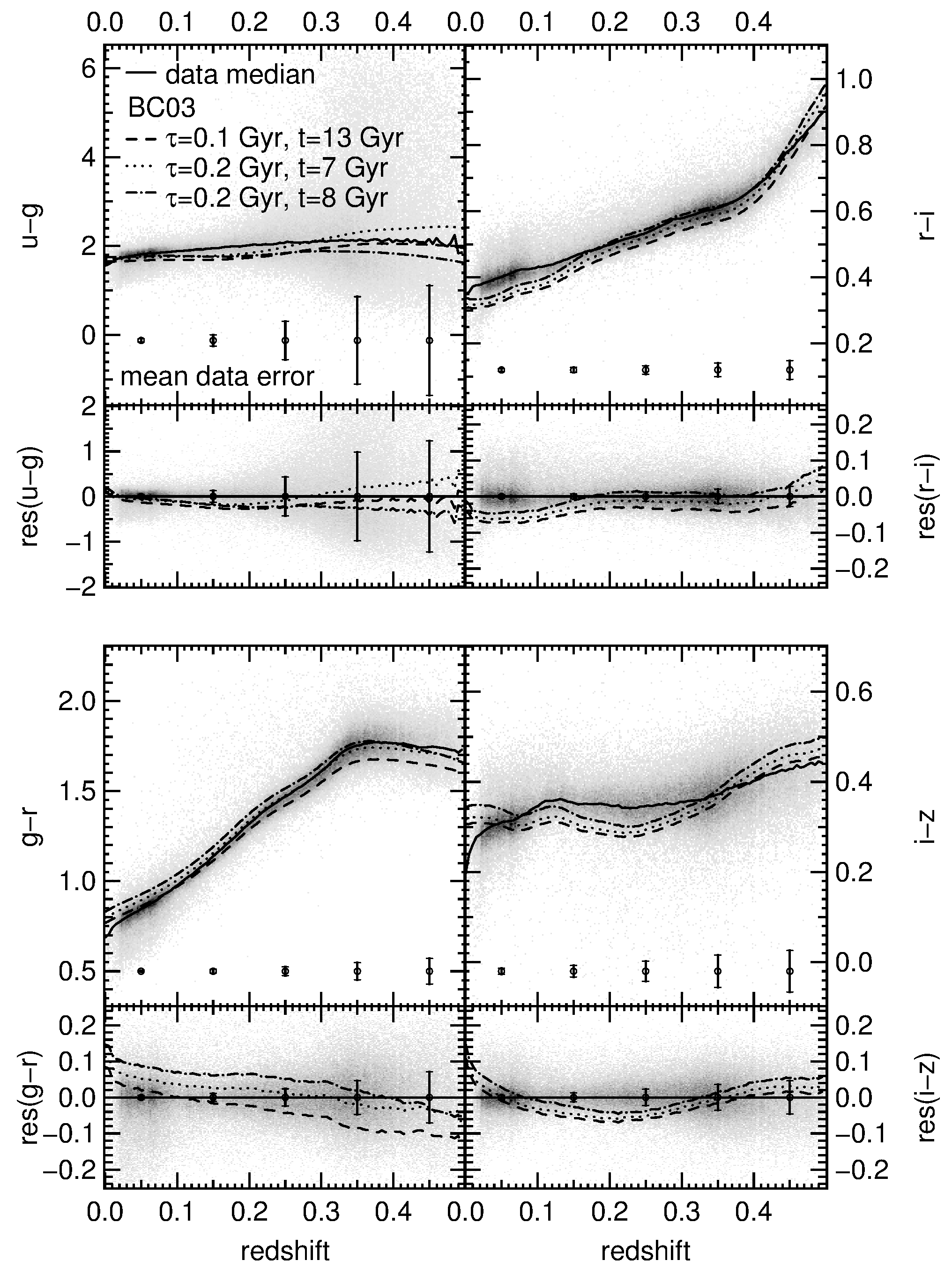
The three best fitting models have and ages of , with and . Their colors are shown as a function of redshift in Figure 2. The best fitting ages and -folding timescales seem realistic, and reflect that the red colors of LRGs originate from both shorter and higher ages. All three investigated models show a reasonably good match in the color, but are too red in at lower redshifts, and too blue at higher . Their color is bluer than the data at very small and deviates toward redder in the higher range. Finally, in they are too blue within , and too red for small .
3.2.3 BPZ Models
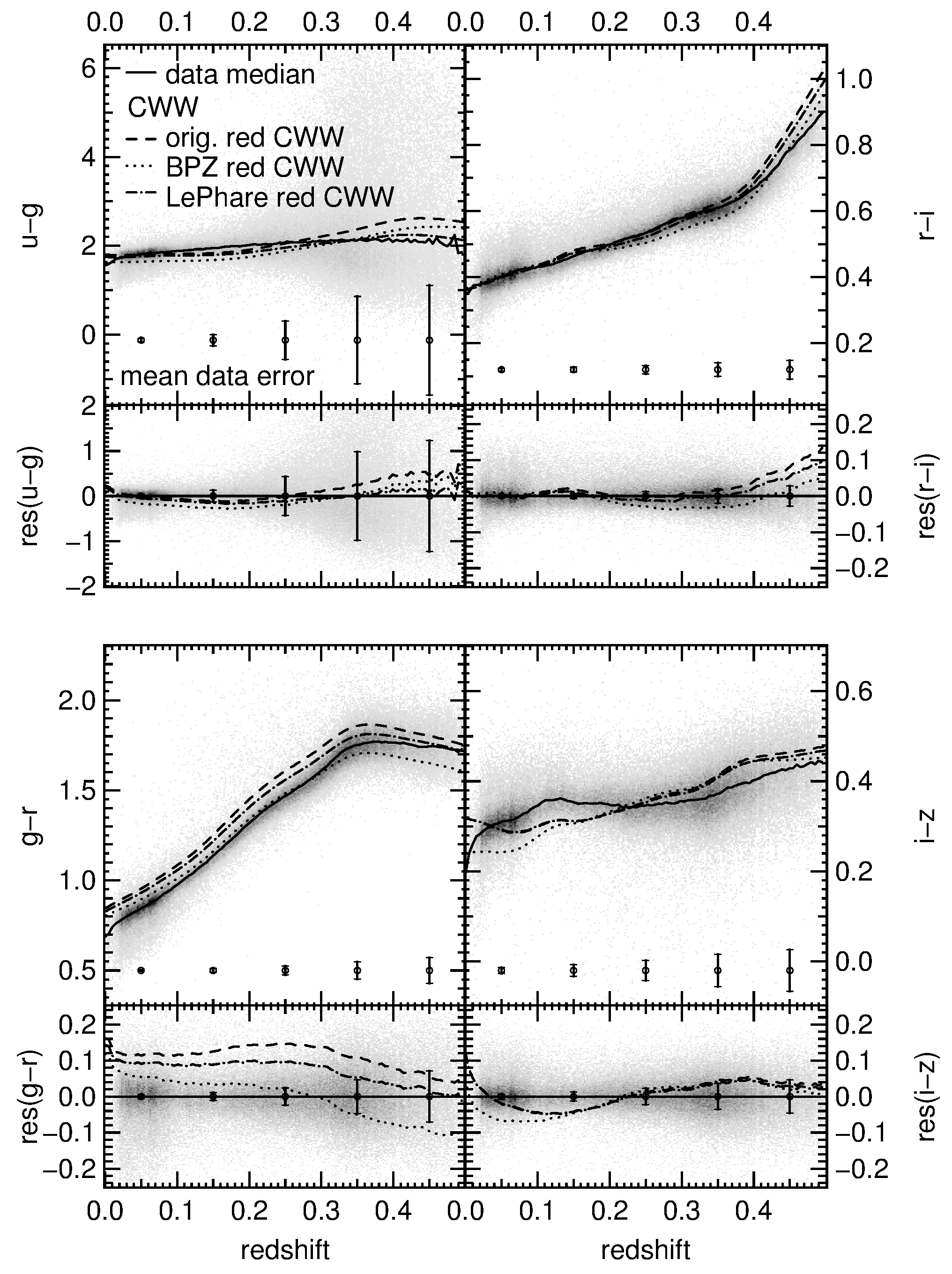
The “Bayesian Photometric Redshift” (BPZ) code333v1.98b: http://acs.pha.jhu.edu/~txitxo/444v1.99.3: http://www.its.caltech.edu/~coe/BPZ/ (Benítez, 2000; Benítez et al., 2004) provides a variety of template SEDs. One is the mean spectrum of local elliptical galaxies by Coleman, Wu, & Weedman (1980, hereafter CWW), which was extended to the UV by Benítez (2000) through linear extrapolation, and to the near-IR with synthetic templates of GISSEL. Extinction was accounted for following Madau (1995). The current version of BPZ (Benítez et al., 2004) includes a repaired version of this elliptical SED, which was calibrated with an array of ground based data. The colors of both the original and the repaired red CWW SED, are shown in Figure 3. Both match the data well in and , with the exception of the latter for higher . There are deviations from the data in over the whole considered range, except for for the original CWW SED, and for medium redshifts for the repaired version. Furthermore, they are able to match the data median in only for medium and high redshifts.
3.2.4 LePhare Models
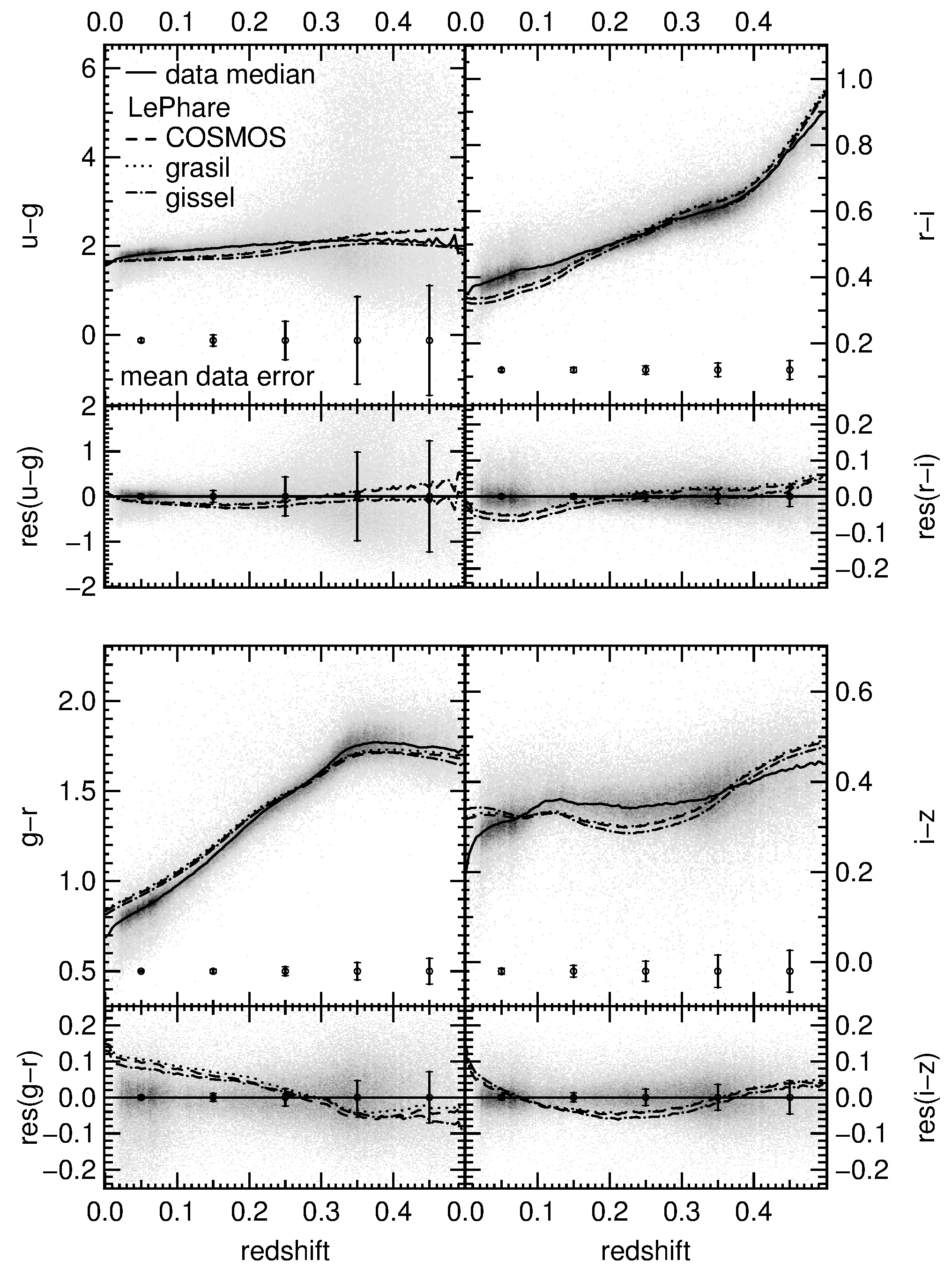
Another Bayesian photo- software is LePhare555http://www.cfht.hawaii.edu/~arnouts/lephare.html (Arnouts et al., 1999; Ilbert et al., 2006), which uses a wide range of template SEDs. We adopt the nomenclature of the models used within the LePhare code in the following. Again, we investigate only red SEDs that produce the smallest residuals from the data according to Eq. 2. The SED delivering the lowest residual originates from CWW models. It was generated by a linear interpolation of the four CWW SEDs and a star-forming galaxy that was constructed with the population synthesis code of Bruzual & Charlot. The resulting colors of the interpolated red CWW SED are shown in Figure 3 together with the colors of the original red elliptical CWW SED and its repaired version of BPZ. Its colors are very similar to the original model and the repaired BPZ version, which were investigated in the last section (Figure 3). The fact that these observationally created SEDs can reproduce the LRG colors well, and are therefore in principle well suited for photo- estimations, was also pointed out by Benítez (2000). Figure 4 shows the colors of three other SEDs that yield the second, third and fourth smallest residuals from the data. The one termed COSMOS is from the LePhare set called COSMOS_SED. Models from this set were used in Ilbert et al. (2009) for photometric redshift estimates in the COSMOS field. The model tagged grasil is a old elliptical galaxy that was created with the GRASIL code (Silva et al., 1998). The SED describing the data fourth best comes from the LePhare 42_GISSEL set. It has an -folding timescale of , a metallicity of and an age of . From Figure 4 one can infer that the colors of those three models are redder than the data for low . In , the three model SEDs are too blue for lower redshifts. Their is redder than the data at and , and bluer at
3.2.5 Models of Maraston et al. (2009)
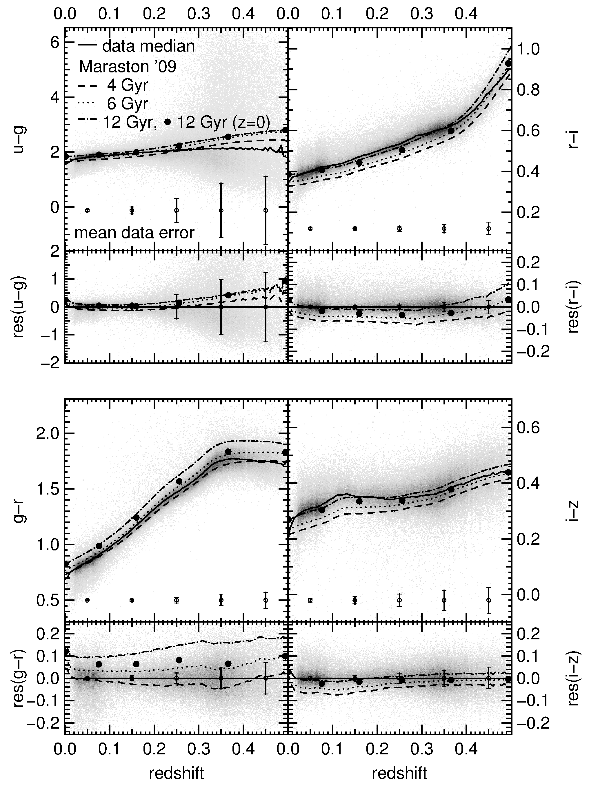
Maraston et al. (2009) already addressed the problem of the color mismatch between model SEDs for LRGs and the actual data. They studied several SEDs and compared them to the data median, focusing on and , and discovered that neither the synthetic nor the empirical SEDs could accurately represent the data at all redshifts equally well. To produce new models that resemble the color median of the data more precisely, Maraston et al. added a mass fraction of 3% blue metal-poor stars to create empirically corrected CSP models. It enabled them to match the data colors considered in their publication ( and ) very well. We present the colors of a subset of the M09 model SEDs666http://www.icg.port.ac.uk/~maraston/Claudia’s_Stellar_Population_Model.html in the , , , and colors in Figure 5. The models that are displayed by lines have not been evolved with look-back time. The SED with an age of yields the smallest residual (according to Equation 2) to the data. It increases faster when turning to younger populations than it does for older ages. In order to show the behavior for ages different from , we display one older () SED in Figure 5, and one younger model with an age of . In contrast to the SEDs examined above, the M09 redshift–color relation has the same shape as that of the data median. The color deviation of the M09 models from the data lies well below the mean error, and does not differ notably for the models with and . At the color of the SED resembles that of the other two SEDs but has lower values for higher redshifts. The color of the old LRG is close to the data at low () but deviates at . Its and colors are too blue in comparison with the data at and respectively. The old SED matches the data in well for and in for all , whereas its color is too red in the whole redshift range. The LRG with an age of is bluer with respect to the data in at all redshifts and at , as well as in at intermediate redshifts (). Unsurprisingly, the older SEDs represent the data at lower redshifts better, while the younger population exhibits colors matching better at higher . An exception is where the oldest model shows an offset from the data, whereas the old model fits well up to . The SED with an age of matches the data reasonably well in throughout the whole redshift range. Figure 5 shows furthermore the M09 model with an age of at evolving with look-back time. The dots at higher represent ages of , , , , and . The colors of the redshift-evolved M09 model are in very good agreement with the data compared to the previously investigated model SEDs. However, the model which is old at and evolves with redshift exhibits an overall offset from the data median in , and has a bluer color for . Furthermore, it deviates in at higher redshifts (), but still lies well within the errors.
3.2.6 Summary
Altogether, we conclude that we could not find models that are able to represent the SDSS LRG data within their errors at all redshifts. The reason for this is that the SEDs differ from the data median as a function of . The M09 models (not taking evolution with look-back time into account; shown with lines in Figure 5) describe the SDSS LRGs best compared to the templates examined before, but they also suffer from notable deviations within some redshift intervals. The lower redshift range () and the colors were not considered in Maraston et al. (2009). As expected, the colors of the redshift evolved SED with an age of at (solid circles in Figure 5) match the data better as a function of redshift, although not perfectly. Furthermore, if only the age of a SED is varied, one just obtains a one-dimensional sequence in color–color space. Instead, the colors of true SEDs are spread in two dimensions, which is a clear hint that not only the age of the LRGs, but also the SFH, and maybe metallicity, vary. A wider spread can thus only be produced if different SFHs and metallicities are considered, which are not publicly available for M09 models. We therefore conclude that in order to get SEDs which represent the data at all redshifts and in all colors, one has to consider different SED template sets for different redshift bins.
4. New SED Templates
In the past, optimal template SEDs have been obtained by “repairing” individual SEDs empirically using the mismatch of observed and model colors (e.g., Csabai et al., 2003). In addition, or alternatively, a larger variety of template SEDs has been obtained by interpolating between a smaller number of template SEDs (e.g., Brammer et al., 2008). However, there are some caveats. If models that one starts with are a bad match to the data it is unlikely that a combination of them will be any better. Moreover, if one introduces SEDs that do not match the data, one deteriorates the photometric redshift quality. Furthermore, the question of how many SEDs are needed to match the data remains undecided.
4.1. Generating Best Fitting SEDs for Individual Objects in the LRG Catalog by SED Fitting
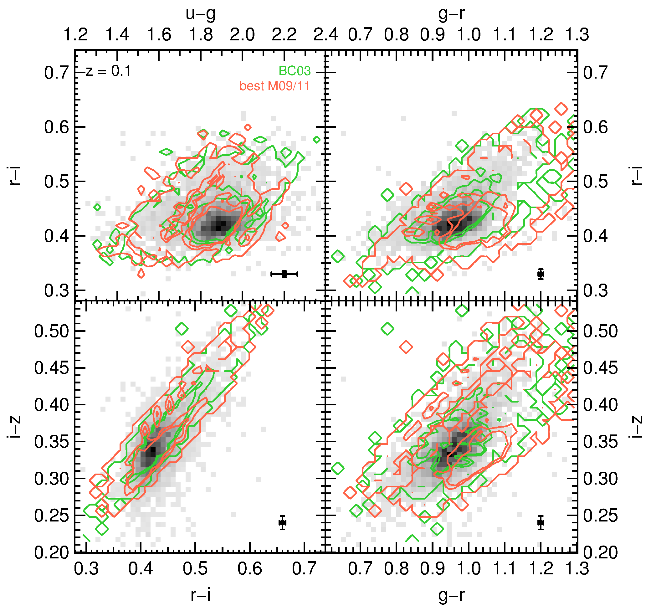
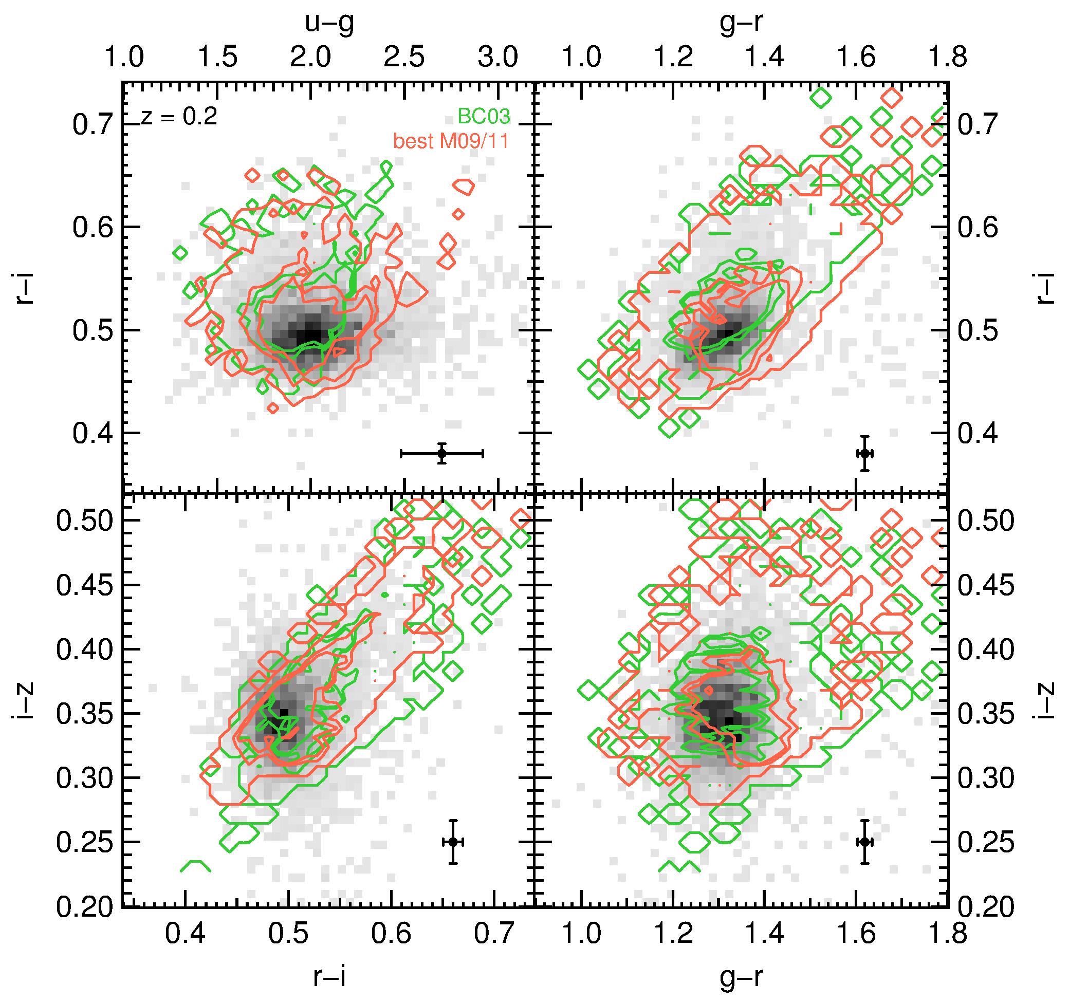
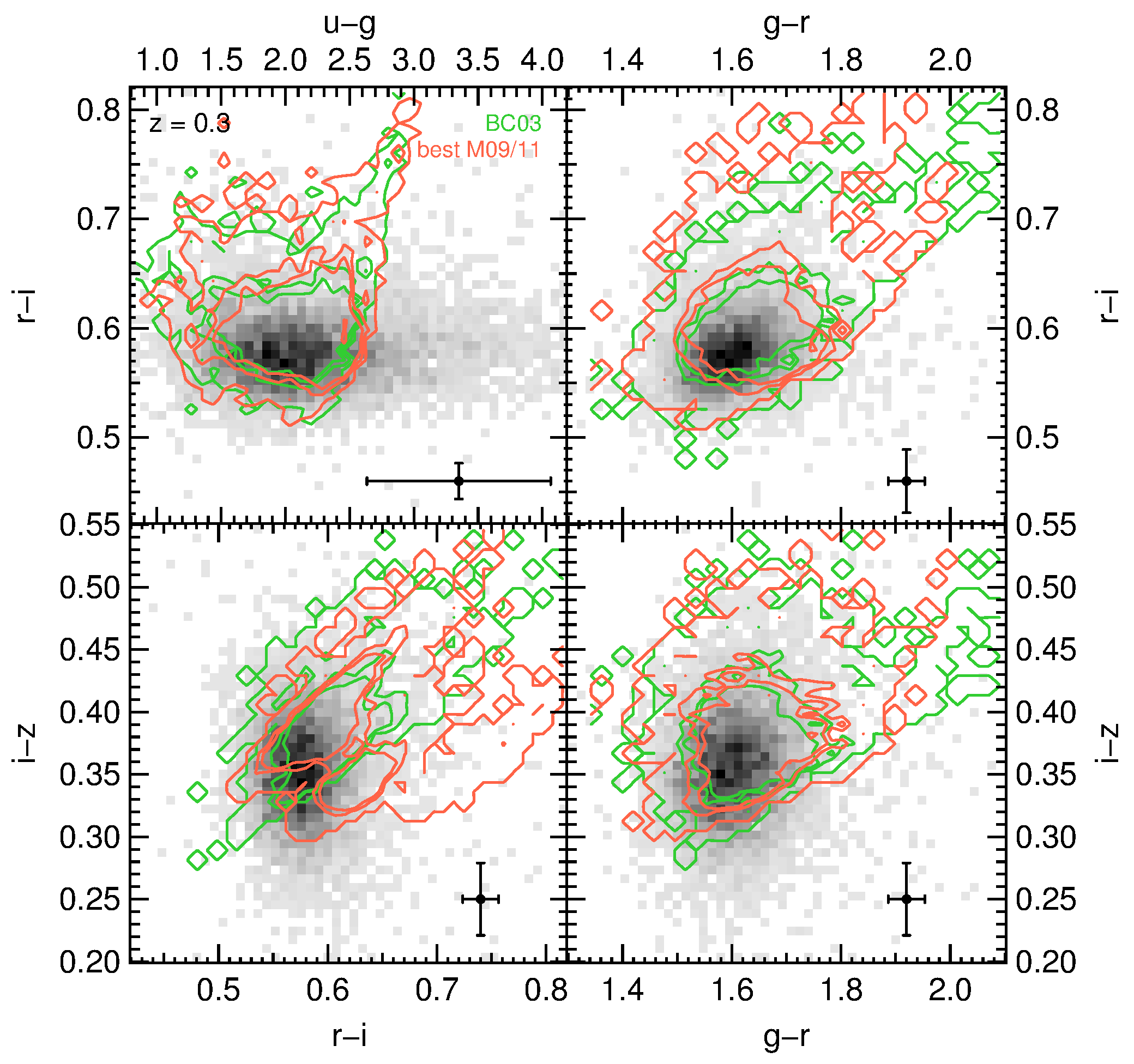
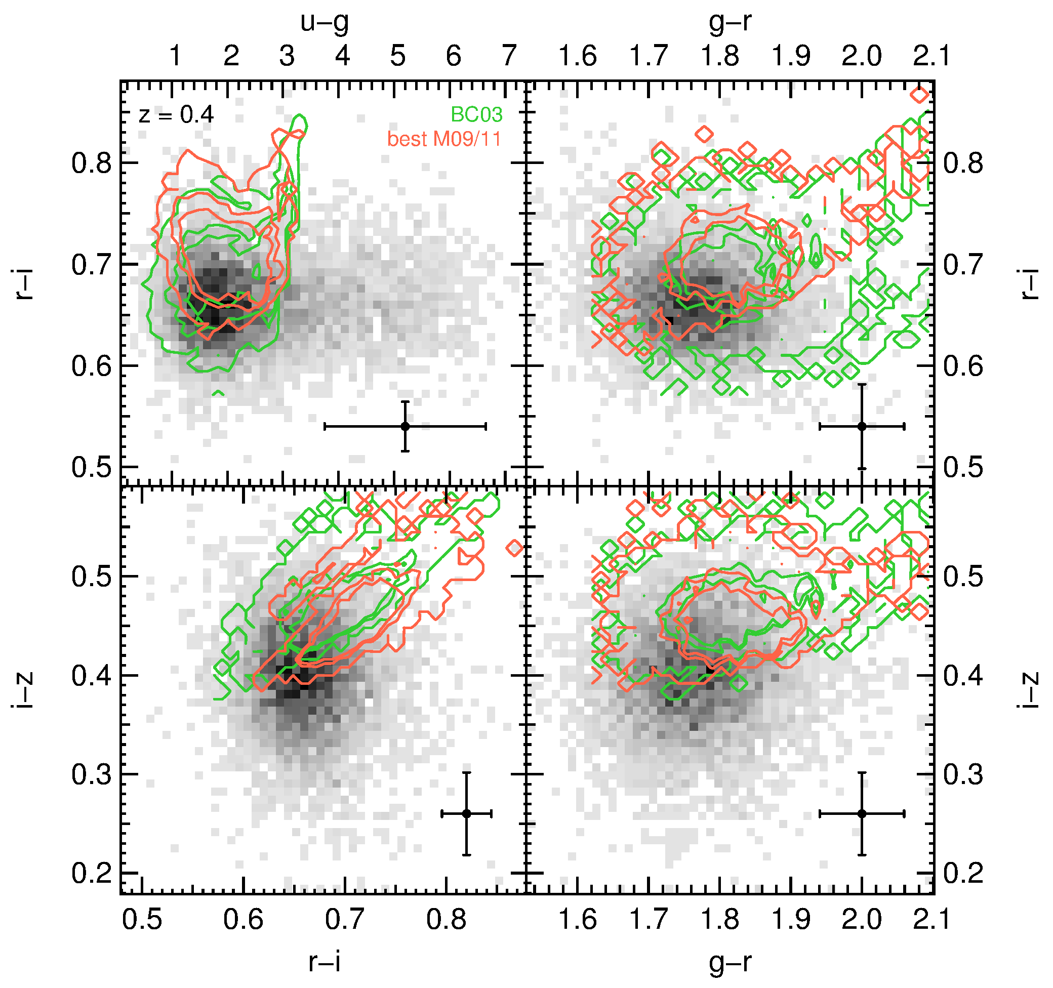
We start with SEDs that match the photometry of individual galaxies as well as possible, and subsequently select a small subset of these SEDs with the goal that they together describe the whole data set. To derive SEDs for individual galaxies, we make use of the largest appropriate freedom to describe a SED with five band data. I.e., we describe the SED of an LRG by a superposition of a CSP and a burst model. Furthermore, we allow for extinction of the CSP and the burst component. The burst and its extinction are physically motivated by the fact that LRGs can contain some young stars. The extinction of the CSP is mainly there to increase the degree of freedom and allows to change the continuum slope (i.e., to introduce a “variance” of CSP models) of the main stellar population. We generate SEDs for LRGs with the SED fitting routine SEDfit (Drory et al., 2004). It chooses the best fitting CSP+burst combination through minimization, concurrently allowing for dust reddening of both components following the extinction law of Calzetti et al. (2000). In Section 3.2 we pointed out that for each model there is always a discrepancy between the model and data colors at some , and we are not able to pick a set of models which describe the data equally well at all . Thus, we create templates specifically designed to represent different redshift regions. We do so by splitting the spectroscopic SDSS LRG sample into five subcatalogs, all of them containing objects within redshift intervals of width , centered on , , , and . These catalogs contain , , , , and objects. They are then divided into two equally sized subcatalogs; one serving for template generation (derivation half) and the other one serving as reference when estimating photometric redshift accuracies (validation half). Subsequently, we run SEDfit with a model set consisting of 864 BC03 models from the BaSeL library (Bruzual & Charlot, 2003) with Padova 1994 evolutionary tracks and an IMF from Chabrier (2003). They have ages between and , -folding timescales of , and to , and four different metallicities, , , and . In order to fit the photometry, these models can be superposed by a fraction of the burst model, with an essentially constant SFR (i.e., ), solar metallicity, and an age of . The burst mass-fraction is constrained to with steps of . Both the CSP and the burst component can be extincted separately. This fitting procedure results in a SED that reproduces the data as well as possible. We end up with one “best fitting SED” for each object in the template generation catalog. The relative performance of SED fitting with models of BC03, M09, and Maraston & Strömbäck (2011, hereafter M11) is demonstrated in Appendix A, where we also justify why we prefer BC03 models over M09/11 for our SED construction procedure. From Figure 19 in Appendix A we conclude that BC03 models allow a better coverage of the colors of the LRGs than M09/11 models do, and fit the data better (Figure 20).
4.2. Selection of Best Fitting SEDs for the New Template Set
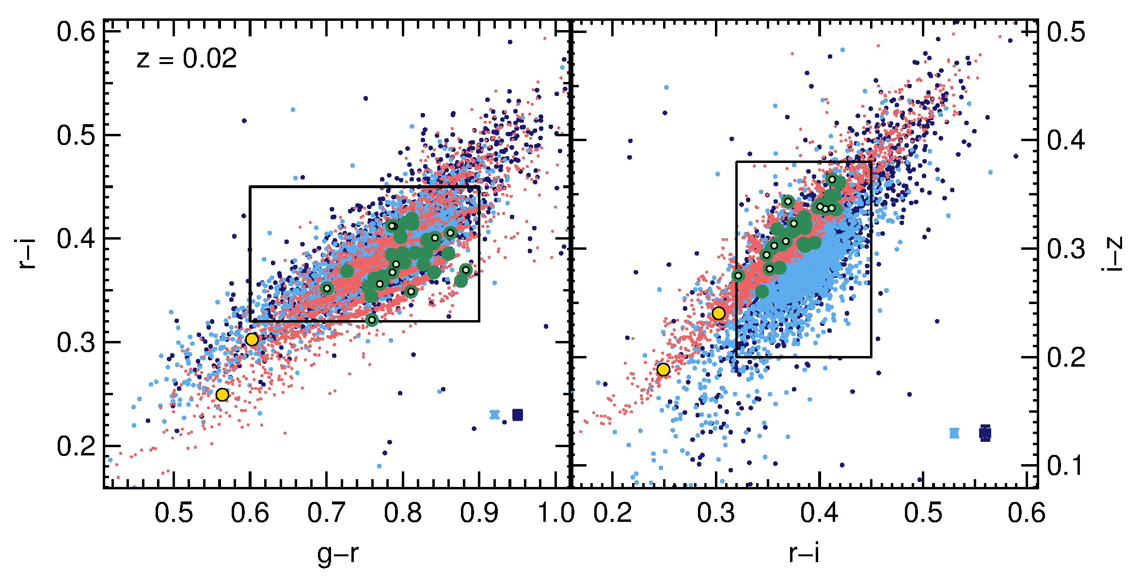
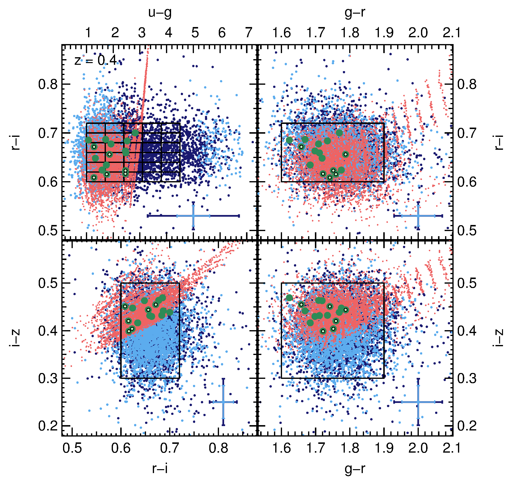
We want to select a set of models from all the SEDs we produced for the template generation subcatalogs such that this set represents the five redshift subcatalogs in color space. We explain our procedure for the redshift interval using Figure 6.
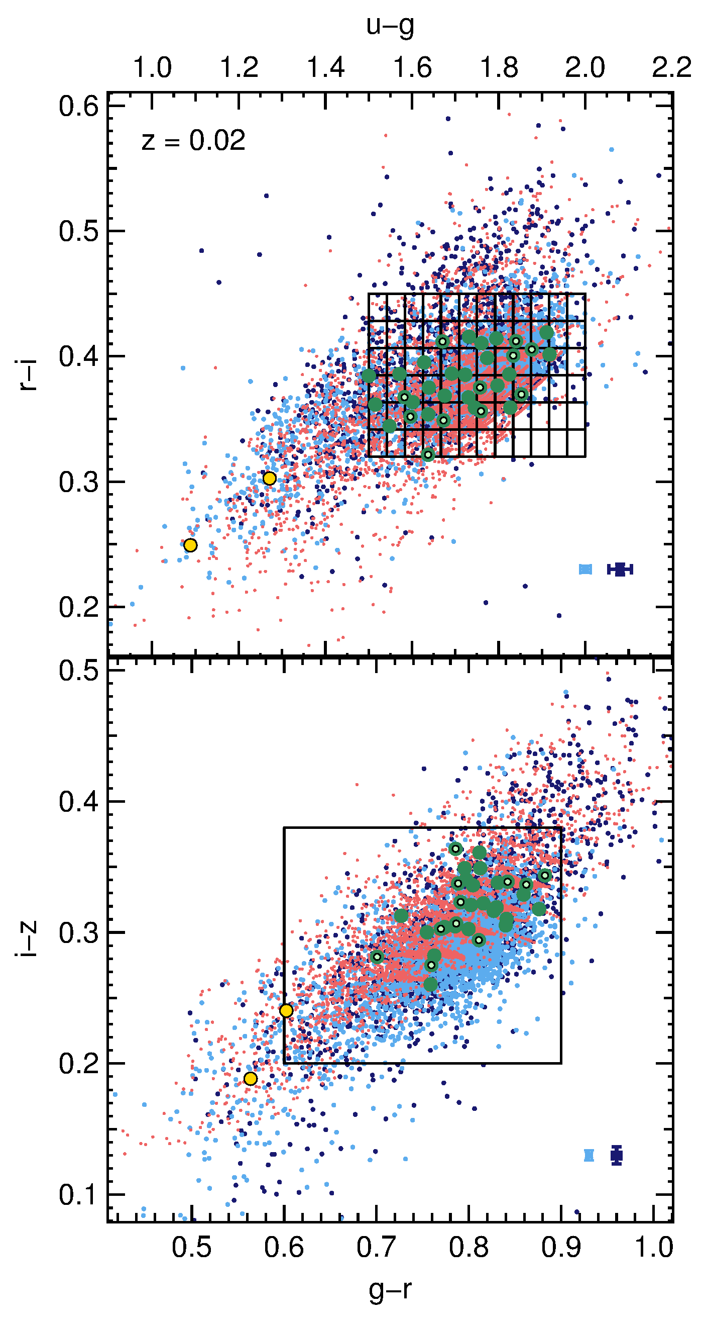
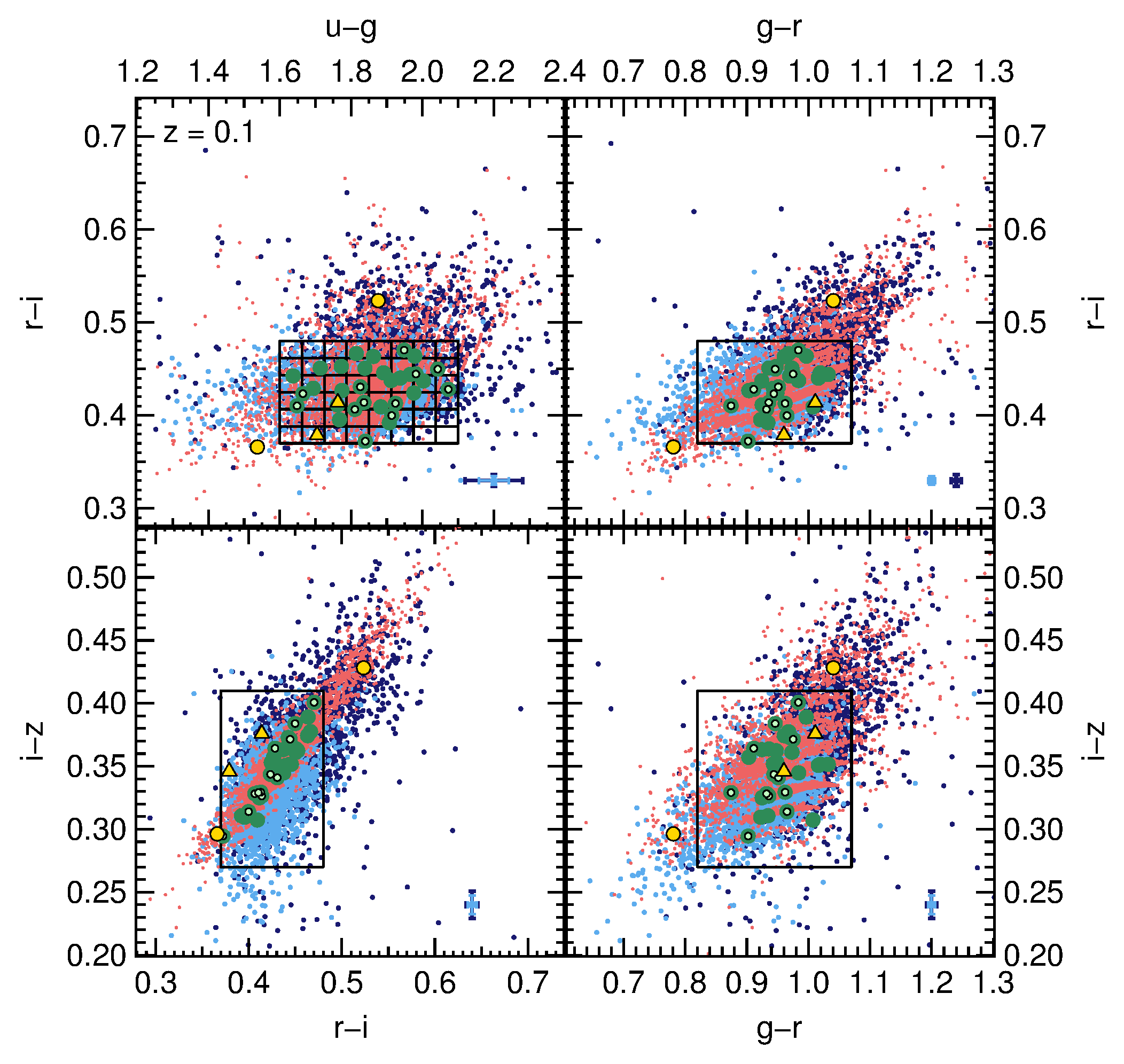
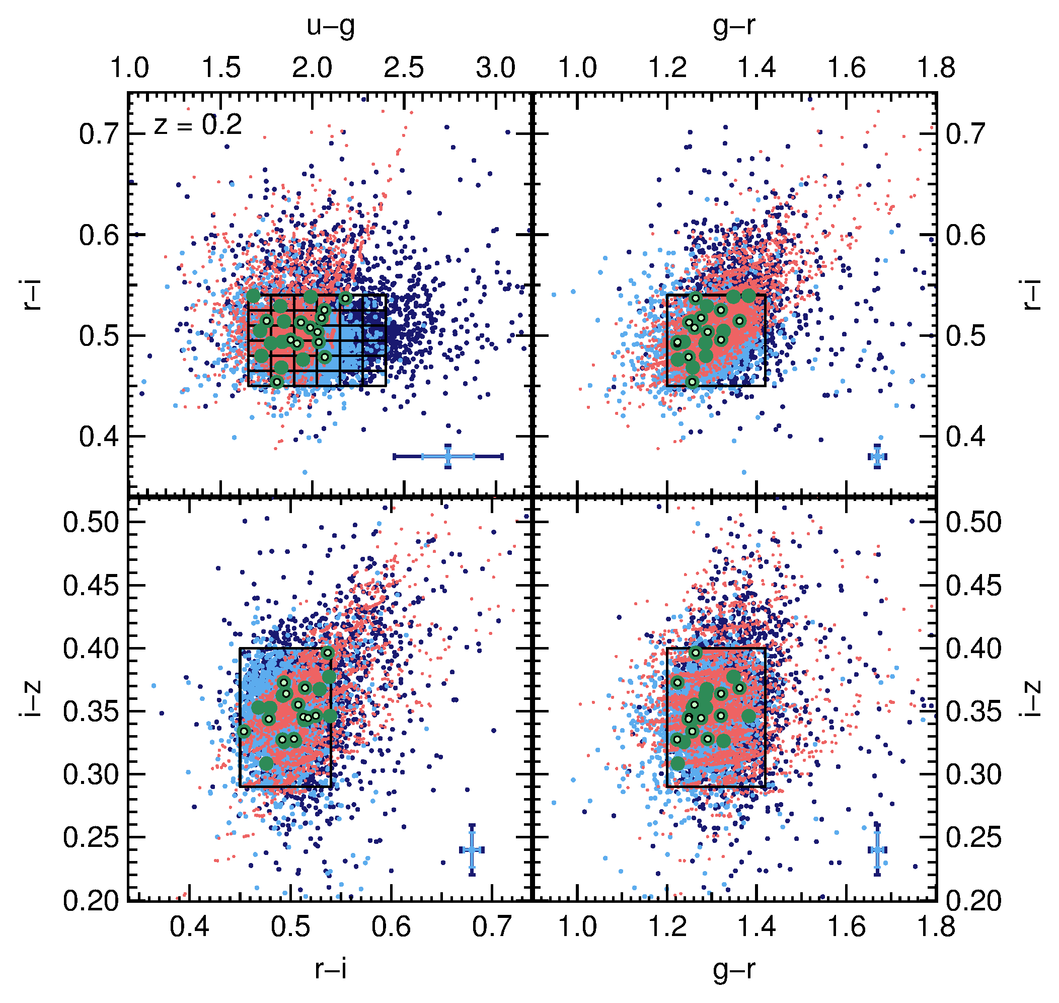
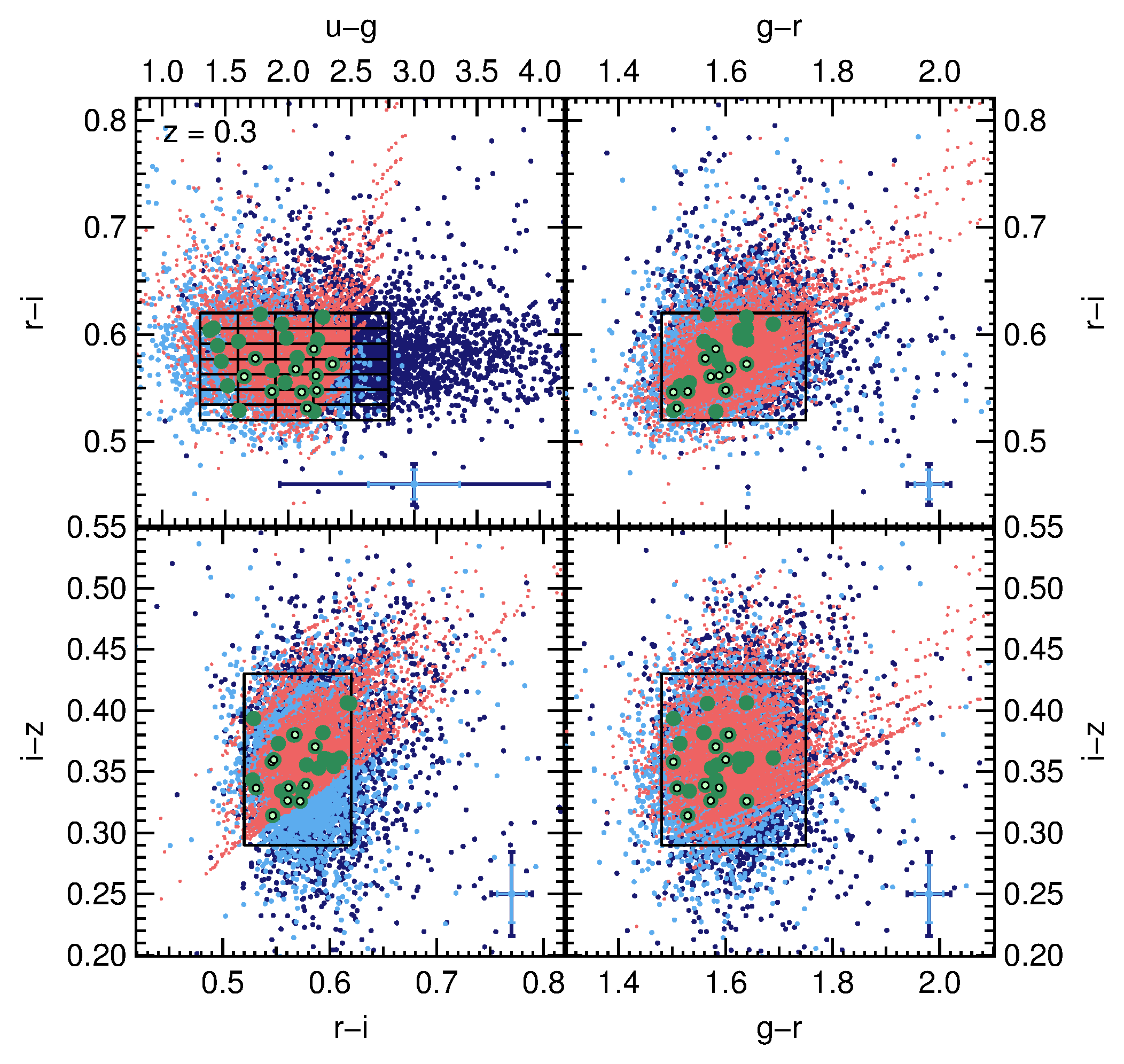
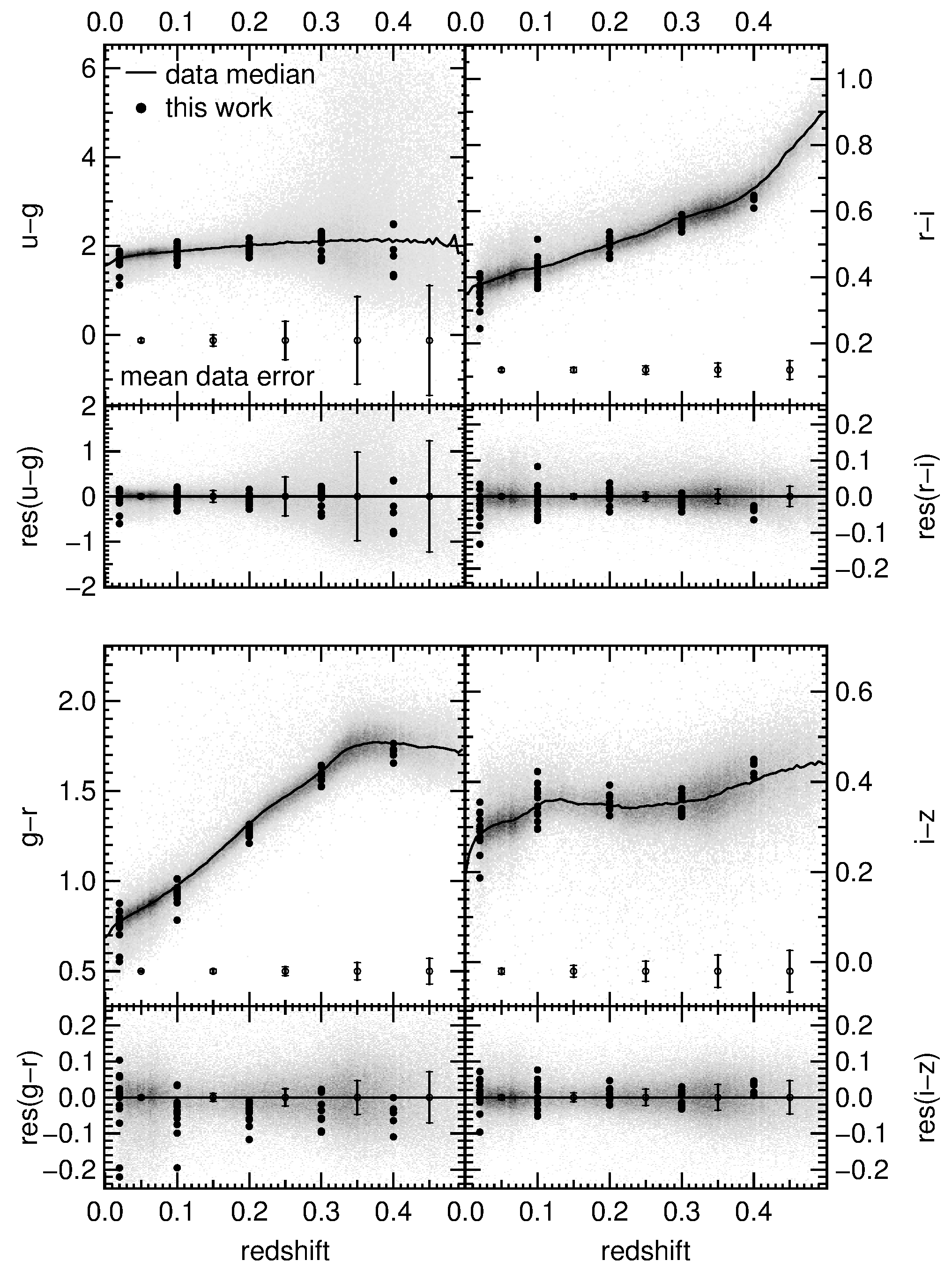
First we plot the distributions of the measured colors of the galaxies in the versus plane. Objects which have a band error smaller (larger) than the median are displayed with light (dark) blue points. Second, we plot the colors of the best fitting SED for each object with red points. If the best fitting SEDs are a good match to the galaxy data, then the distribution of them in color space should be similar to the observed distribution, once the spreading by photometric errors is taken into account. The mean photometric errors for the two subsamples (with high and low band errors) are shown in dark and light blue in the lower right corner of the panels in Figures 6, and 21–25. It shows that galaxies with larger photometric errors in in general also have larger photometric errors in and , which implies that these objects are fainter in all observed bands, rather than just in the band. We conclude from the shown sizes of the mean photometric errors on one hand that the spread in colors is of physical origin, and not due to photometric errors. This also holds for higher redshifts where the error bars are of significant size. In order to confirm that, we simulated galaxy colors by assuming that the spread in color space is a result of the photometric errors only. We simulate the data by assuming that each object in fact has a color value of the average color. Then we assign a random deviation from this point, based on a Gaussian probability distribution with the measured error as standard deviation. Since the spread in the simulated data is smaller than that of the data, we confirm that the spread within the colors is of physical origin. On the other hand, we infer that the color distribution should hardly be broadened by photometric errors, and that the best fit SED color reproduce the variety of ’true’ galaxy colors well. Only for the reddest colors ( and ) we find mostly objects with larger than median photometric errors, such that some of these data points will be scattered out from the true distribution by large photometric errors. We now select model SEDs for the “main galaxy” population. Therefore, we define an area in the -plane which contains the majority of objects (black box), and then set a grid within this area (black grid). The chosen area is selected by eye and was confirmed to include at least of the objects from that redshift bin. We want to select one object per cell which shall represent the other objects within that cell. We carry out this procedure only for cells that contain at least 20 galaxies. From each of those cells we pick the SEDs best fitting the five objects from that cell which have the lowest u band error. As mentioned above, our objective is to produce photometric redshifts with biases as small as possible, and we therefore try to single out SEDs that produce small on the catalogs of the regarded range. Hence, we perform PhotoZ runs on the derivation half and on the validation half of the subcatalog, the latter to confirm that we did not unintentionally divide the catalog into halves with different object properties. We perform the photometric redshift estimation with each of the preselected models separately, thus fitting only one model per run. Afterward, we pick the SED that renders the smallest bias on both subcatalog halves out of the five originating from the same cell. The selected model shall represent the objects within its neighborhood in color space in the following PhotoZ runs. Repeating the same procedure for all cells and redshift bins, we select roughly to model SEDs per bin. In order to save computation time for a PhotoZ run, we want to keep the number of templates to a minimum. Therefore, we calculate the root mean squared flux difference of each SED combination at every defined wavelength. The most similar SEDs are then removed from the final set, leaving typically about models per redshift bin with a total number of templates. The redshift of the models is plotted versus their color in Figure 7. Color–color relations of the new models in comparison to the LRGs are displayed in Figure 6, and Appendix B, Figures 21–25. The templates represent the LRG colors and their spread for most values of . The exceptions at are discussed in Appendix A, Figure 25. We test the performance of the new models with respect to photometric redshifts in the next section. As an alternative we also selected template SEDs with a kd-tree. We generated one hyperplane for each of the four colors , , , and , thus a four-dimensional tree with 16 template SEDs for each redshift bin. One model was selected from each branch of the tree by the same criteria as already described. As this technique yielded SEDs not too much different, we kept our hand-selected set.
5. Photometric Redshift Precision with the Novel Template SEDs
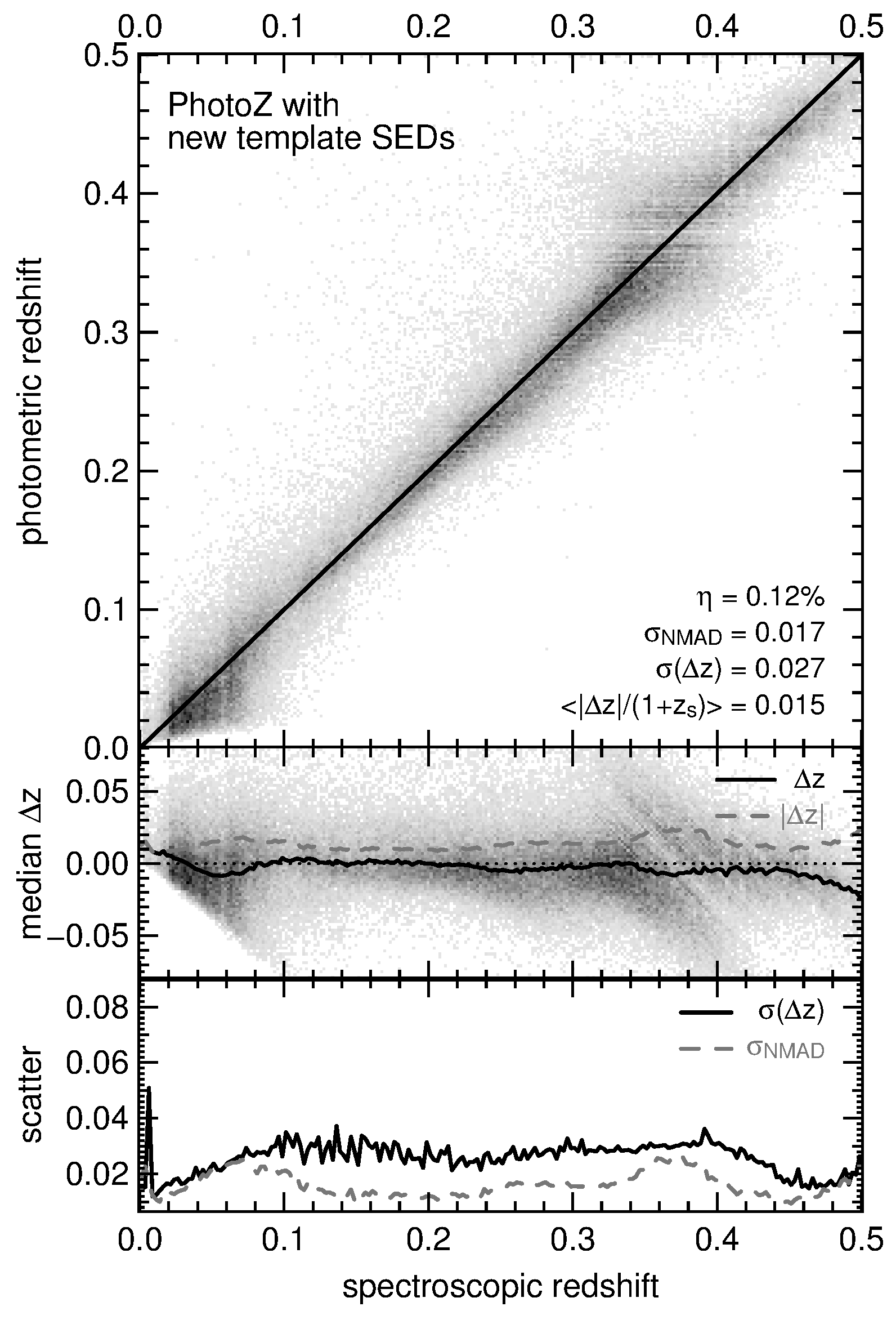
Before analyzing the photometric redshift results we get with the new template SEDs, we introduce some quality parameters. To define badly estimated photometric redshifts we use the threshold introduced by Ilbert et al. (2006). Objects that fulfill this inequality are tagged “catastrophic outliers”, and their number fraction will be called . shall denote the root mean square of the photometric redshift error . A parameter that quantifies the distribution perpendicular to the line without the inclusion of catastrophic outliers is (Ilbert et al., 2006). With one can make conclusions about the redshift uncertainty excluding the tails of the distribution. After these definitions we turn to the integration of the newly created model SEDs into PhotoZ. In Section 2 we mentioned the redshift priors we can impose on each template. The total probability for a model- combination is proportional to the redshift probability . As already mentioned in Section 2, we use a Gaussian probability distribution, . In this way, can be set to the according redshift interval’s center for each model, thus . The redshift prior probability of the model is equal to ½ at the corresponding . The photometric redshift results are shown in the upper panel of Figure 8. With the new red templates, the described priors, and a resolution of we indeed get very accurate redshifts. The catastrophic outlier rate is very small at . The dispersions is and respectively. The mean absolute deviation of from is . We show the bias as a function of redshift in the middle panel of Figure 8. It exceeds only for the highest redshifts (). The reason for the small positive bias at is that there are no negative photometric redshifts that can cancel out overestimation. The total mean bias reads . At , the 4000 Å break position in wavelength cannot be determined to high precision. This is because at the 4000 Å break is observed at and thus lies in the gap between the SDSS and filter. We therefore expect that the error distribution widens at this redshift. The reason for the error becoming bimodal is likely because at this redshift we do not have “perfect templates” and thus the photometric redshifts are either over- or underestimated. Luckily the errors nearly average out for every redshift bin. The bottom panel of Figure 8 shows the dependence of the scatter and on . At low () it is up to , which is likely due to contamination of the LRG sample with non LRGs. This is supported by the fact that the values in this region are significantly higher than for . Apart from very small redshifts, the scatter stays more or less the same for all redshifts.
6. Comparison to SDSS Database Results
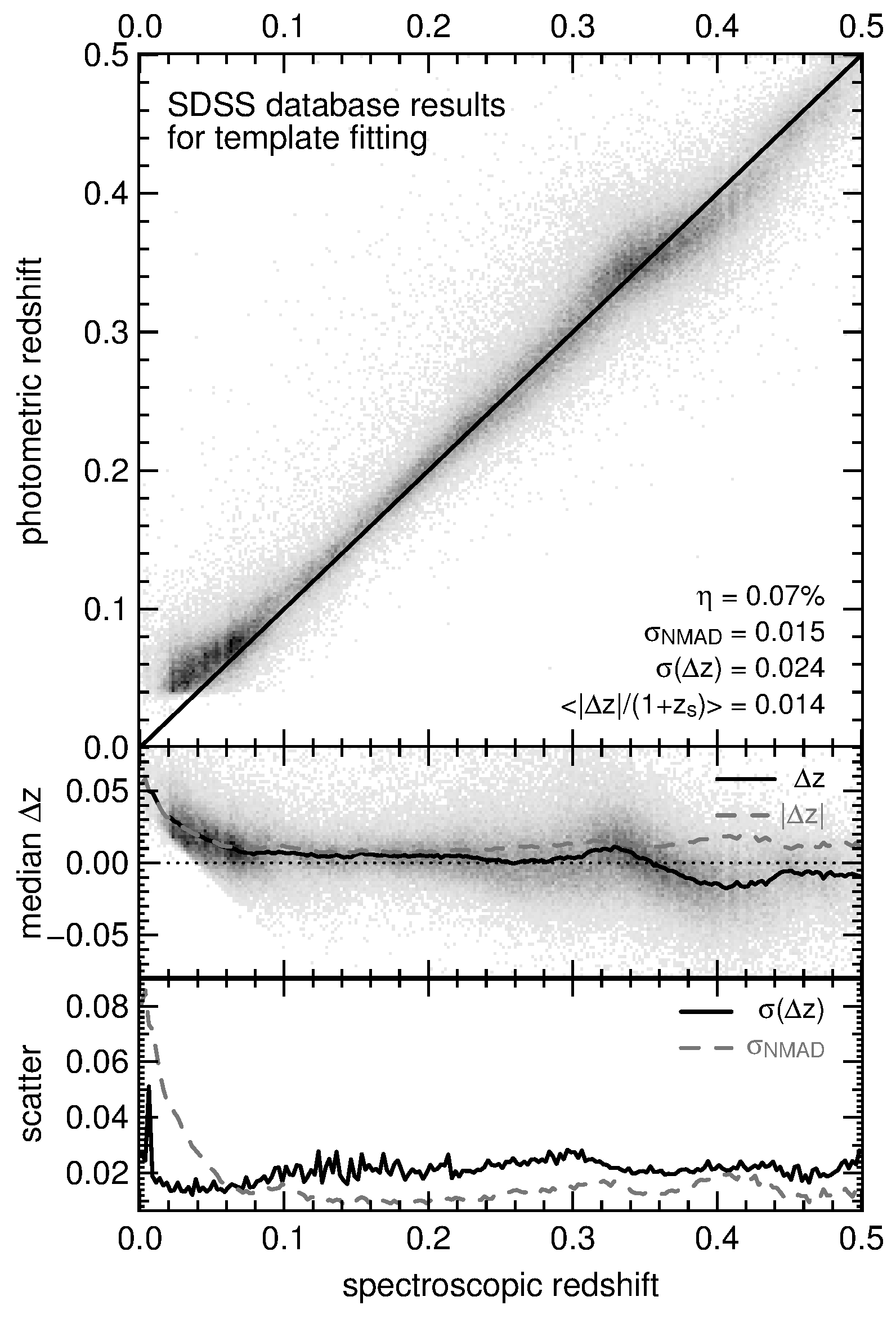
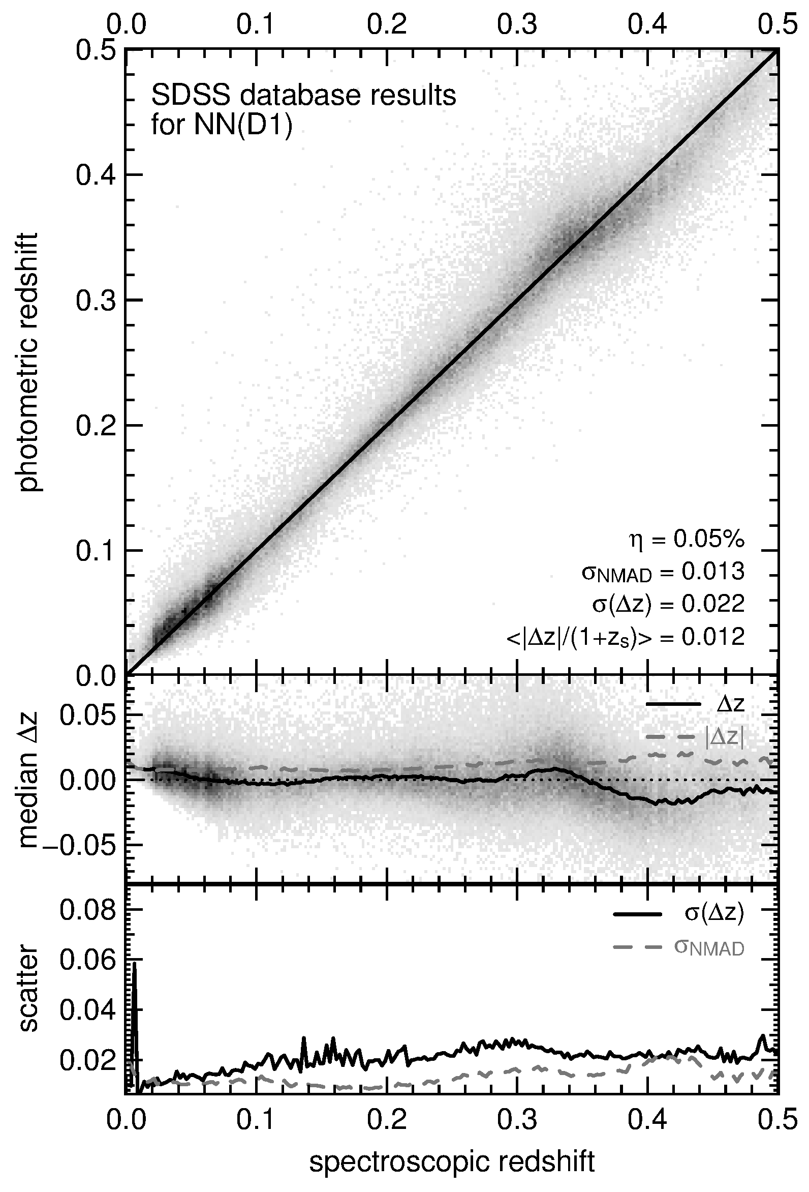
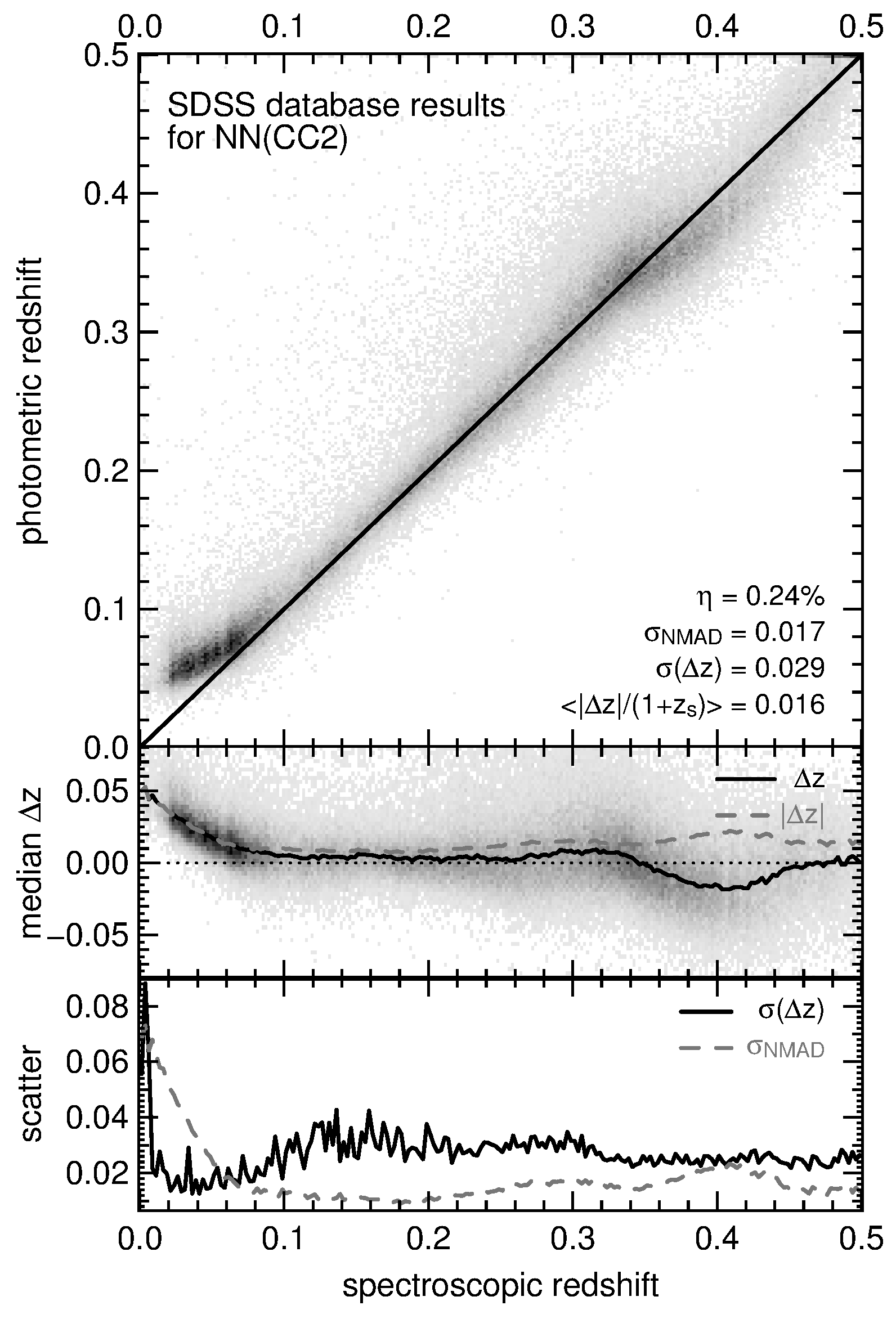
We now compare our photometric redshift results with those in the SDSS database. There are three kinds of photometric redshifts available in the database: One was obtained through template fitting (i.e., a hybrid technique of template fitting and a reparation of templates, see Csabai et al. 2003), and the other two are results of an artificial neural network (ANN) approach (Oyaizu et al., 2008). The results of the template fitting are shown in Figure 9. On average, the and of these redshifts are smaller than for our method, but the bias is more unevenly spread in redshift space. Also for this method the median bias is smaller than only in the redshift range of . For other redshifts the bias exceeds that of our redshifts considerably. The SDSS database values for photometric redshifts obtained with the ANN are shown in Figures 10 and 11, where we display the results of two techniques, D1 and CC2. The ANN(D1) method uses ugriz magnitudes and the concentration indices of all five bands for the determination of photometric redshifts. A concentration index of a passband is defined as the value of the ratio between the radii encircling and of the Petrosian flux. The CC2 approach on the other hand is based on the , , , and colors and the concentration indices in the g, r and i bands. Photometric redshift results are shown in Figures 10 (D1) and 11 (CC2), respectively. The ANN(D1) performs excellently in terms of scatter and bias from to , but it yields a considerably larger bias than our redshifts for . Photometric redshifts from the CC2 method are significantly overestimated for , where the bias exceeds . Additionally, the is particularly high at small spectroscopic redshifts (), which is probably due to the overestimation in this range. At , surpasses , whereas at intermediate redshifts, the photometric redshifts from the ANN(CC2) are slightly overestimated. We conclude that PhotoZ with the new set of LRG templates delivers results competitive with empirical approaches.
7. Properties of the Novel Template Set
In this section we want to discuss the properties of our new template SEDs in the UV wavelength range and analyze how well they represent objects with UV data. Being able to match the UV colors of observed objects justifies that we discuss the novel SEDs from a physical point of view and with regard to the underlying galaxy population in Section 7.2.
7.1. UV colors of the Novel Templates and M09 Models
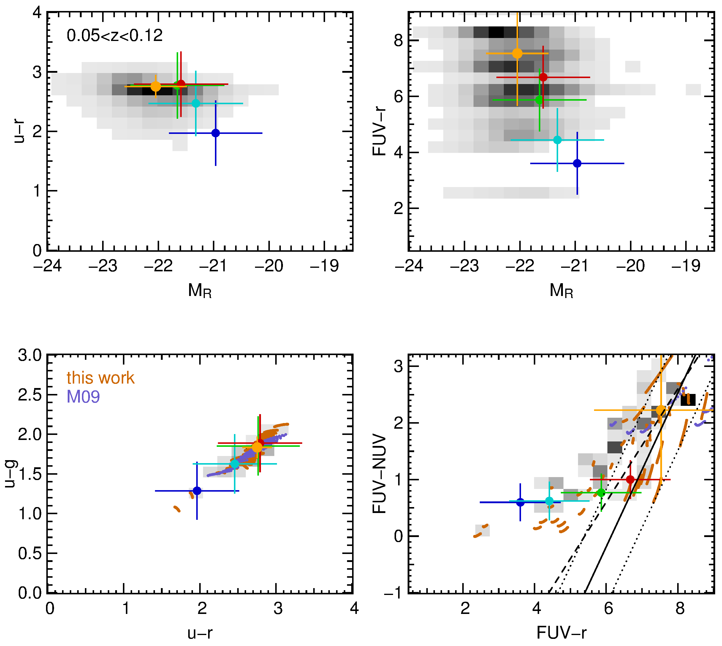
We show color–magnitude and the color–color relations of our final template SED set down to UV wavelengths within and compare our findings to those of Ree et al. (2012, hereafter R12). We want to evaluate if the novel models are able to represent the Galaxy Evolution Explorer (GALEX) data, since we used no information about the UV in the creation of our SEDs, as even the GALEX NUV filter central rest frame wavelength is at a redshift of , whereas the SDSS band filter has a much larger central wavelength of . R12 selected ETGs in the SDSS data on the basis of morphology, requiring , and removed contamination by late-types through visual inspection. The sample galaxies were then classified into quiescent, star-forming, composite, and active galactic nucleus (AGN) categories on the basis of their emission line characteristics. Quiescent ETGs were selected in such a way that they do not exhibit emission lines. Figure 12 shows the data medians and their spread of the four ETG categories of the galaxy sample of R12 in color–magnitude ( versus and versus ) and color–color diagrams ( versus and versus ) in analogy to Figure 1 in R12. Additionally, we plot the colors and magnitudes of our final templates after fitting them to the spectroscopic redshift of the LRGs within , as well as their intrinsic colors within that range. The median values of and coincide with those of the quiescent and AGN ETGs of R12 (lower left panel), and we are able reproduce the observed UV-colors. on the other hand is about lower in this work when compared to the quiescent and AGN ETGs of R12 (upper panels), visualizing that the objects in our sample are definitively LRGs. Furthermore, the median UV excess () of SEDs of this work is significantly smaller than that of R12 ( compared to the quiescent galaxies; upper right panel). The lower right panel displays the UV-excess versus , as well as the UV red sequence found by R12 (solid line) which is derived empirically through a linear fit to the observed colors with width (dotted lines). A fraction of our models however lie above the UV red sequence. Also the color is higher than in R12, due to the fact that our models have higher fluxes in the band and lower fluxes in . According to Schawinski et al. (2007), recently star forming (RSF) galaxies fulfill the semi-empirical criterion , which is plotted in Figure 12 (dashed line). A considerable part of our models is thus classified as RSF. The lower panels of Figure 12 show M09 models on top of the SEDs of this work. In comparison to R12, M09 models neither cover the region of higher UV-excess (), nor those where , and nearly all of them exhibit no RSF following the criterion of Schawinski et al. (2007). M09 models account for passive evolution only, which is why they do not populate these RSF regions. However, the M09 SEDs match the versus colors of quiescent, AGN and composite ETGs from R12. Nevertheless, at low redshifts the LRG sample consists not only of passively evolving galaxies, but shows signs of recent star formation. M11, which have a large variety of SFHs, ages, and metallicities, should be able to cover these regions.
7.2. Differences in the SEDs within Bins
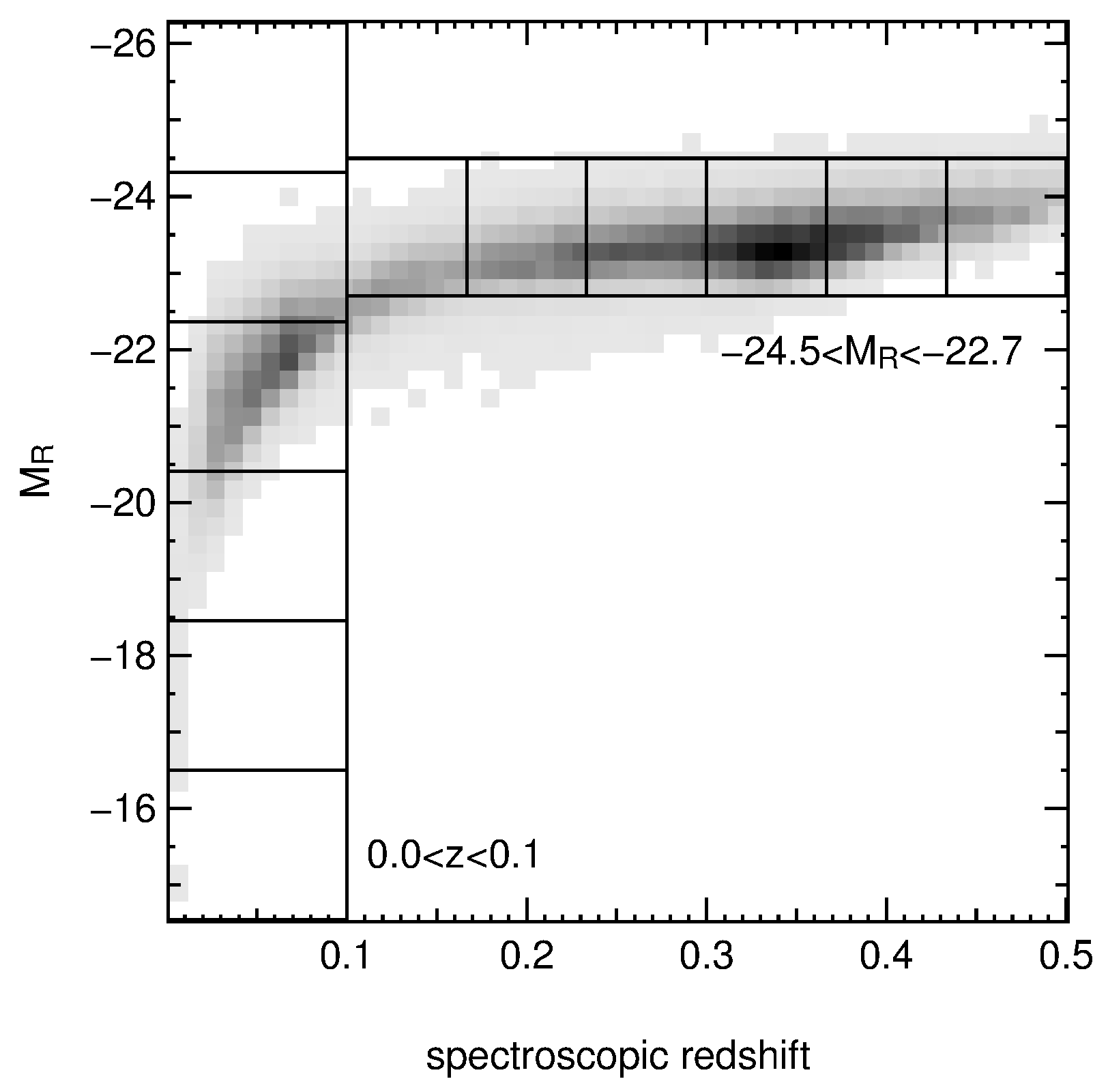
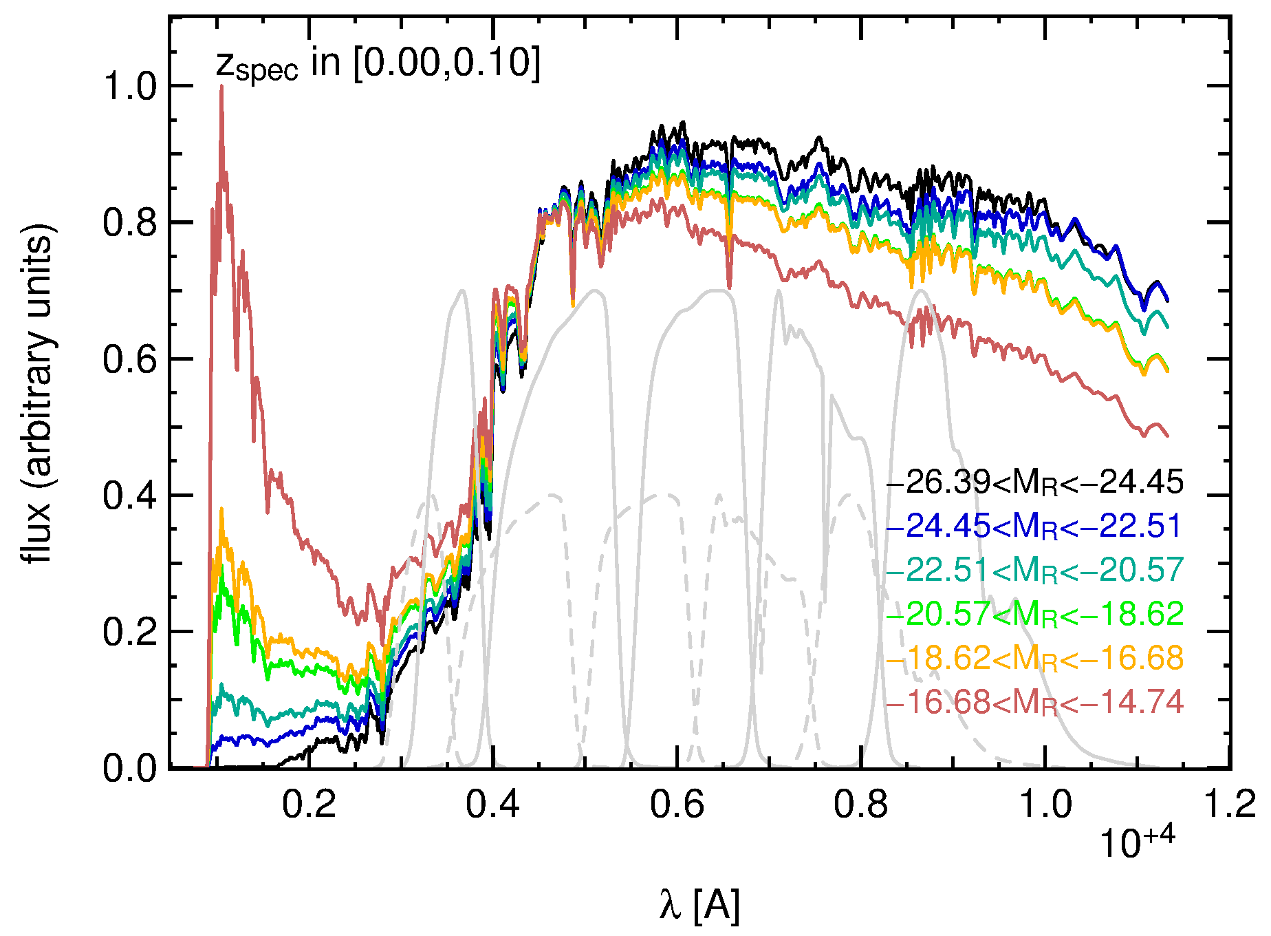
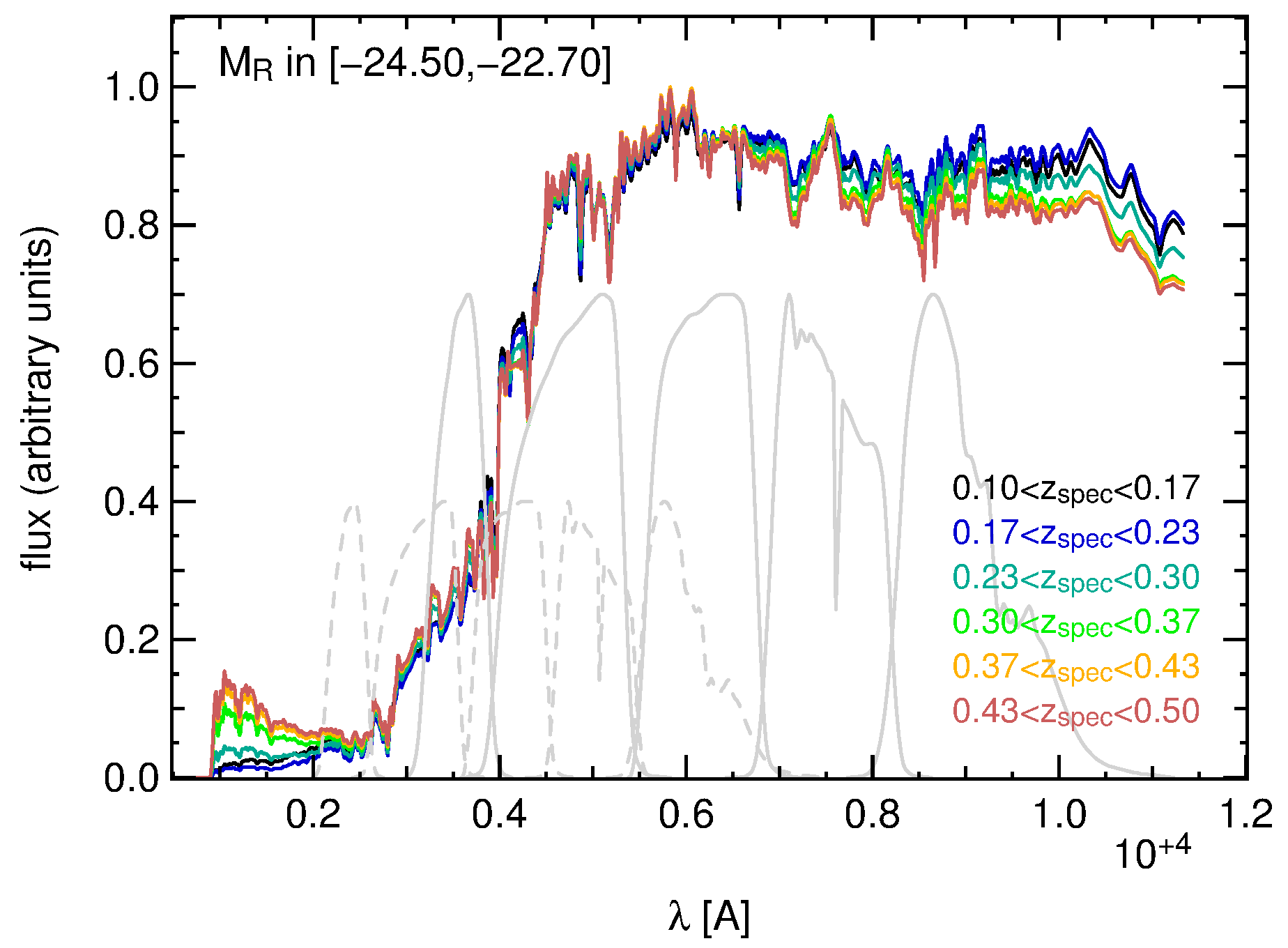
By construction our new template SEDs do not necessarily consist only of old CSPs (which are necessary to match the 4000 Å break of the LRGs), but can have imprints of young stellar populations (i.e., more UV-excess relative to old populations) and dust extinction, changing the slope of the CSP and the burst. Instead of examining what kind of combination the LRGs are fitted by, we present how different the SEDs of galaxies are when matched by our templates. Therefore, we determine the best fitting SED for every LRG by fitting our new SED set at the spectroscopic redshifts of the objects and calculating the absolute magnitude in the R band filter thereafter. We then bin objects within the versus plane (Figure 13) and calculate the mean SED of that bin, by adding up all best fitting SED templates of objects from that bin with weights given by their flux in . Doing this for different redshift and luminosity bins, we obtain the luminosity weighted light distribution of all objects within a given redshift and luminosity range, under the assumption that they are well described by one of the SEDs from our template set. The results for luminosity bins with are shown in Figure 14. The SEDs which match the SDSS data best show a strong dependence on the brightness of the object: The fainter galaxies are, the more flux they have at relative to the brightest bin, and the steeper the slope of the SED gets for on average. Both observations can be explained by star formation in these galaxies, i.e., that low mass LRGs still build stars at low in contrast to the more massive LRGs. Hence, the diversification in the color is not reached by simply selecting smoothly varying SFHs, but rather by adding to these single starburst events of different amounts. We will confirm this result in Section 7.2.1. Figure 15 shows the superposition of the models for and in six consecutive redshift bins. At blue wavelengths () the SEDs from objects at higher redshifts exhibit more flux than those at lower redshifts, which indicates increasing star formation turning on to higher . These effects are in accordance to what one would expect for older stellar populations at low and younger objects at higher . Older red populations have (nearly) completed star formation and hence show low fluxes in bluer bands, whereas their fluxes in the red () exhibit a smaller continuum slope compared to younger galaxies. The SED from the first redshift bin () is slightly bluer than the following (), because there are still star forming objects within that bin. This can be seen in Figure 13: there are still fainter galaxies in this bin, wherefore not all of them are passively evolving. Additionally, Figure 16 in Section 7.2.1 confirms that there are still star forming galaxies in this /-range. In order to support the latter discussion quantitatively, we performed a fit to the variety of BC03 models that are the basis of our template generation in Section 4.1. We keep the metallicity fixed at as well as in order to avoid degeneracies between , , and age. (We discussed these degeneracies in Section 3.2.2.) The best fitting ages for the redshift–luminosity bins at are , , , , , and from brighter to fainter bins. Keeping only the metallicity fixed at , we observe that the best fitting models nearly all have , which supports the claim that they all exhibit ongoing star formation. The first (most luminous) bin has a best fitting of , which is due to the very red SED we calculated for it. Anyway, since this bin contains only one object we cannot assume the SED to be representative, although it would be in good agreement with the sequence the superpositioned SEDs form, and it would not contradict the observation we make in Section 7.2.1 where we deduce from the relations between emission lines that no star-forming galaxies lie in this particular range. We also performed the fitting of BC03 models to the superpositioned SEDs for and keeping at and fixed. The best fitting ages are then: , , , , , and with increasing . As was mentioned above, the first redshift bin () still contains objects with ongoing star formation, which is why the best fitting age is lower than in the second bin (). Nevertheless, the ages from the other five redshift slices are monotonically decreasing. By keeping only the metallicity fixed, the values increase from lower to higher redshift, which also yields to bluer spectra. Furthermore, the differences in the light travel time between the centers of the first and the last redshift bins is , which is in agreement with the fit results, and also supports what we expect when we assume that the underlying population of our sample at predominantly consists of passively evolving galaxies, and that the variations in the SEDs are a result of aging.
7.2.1 Comparison to SDSS Star Forming LRGs
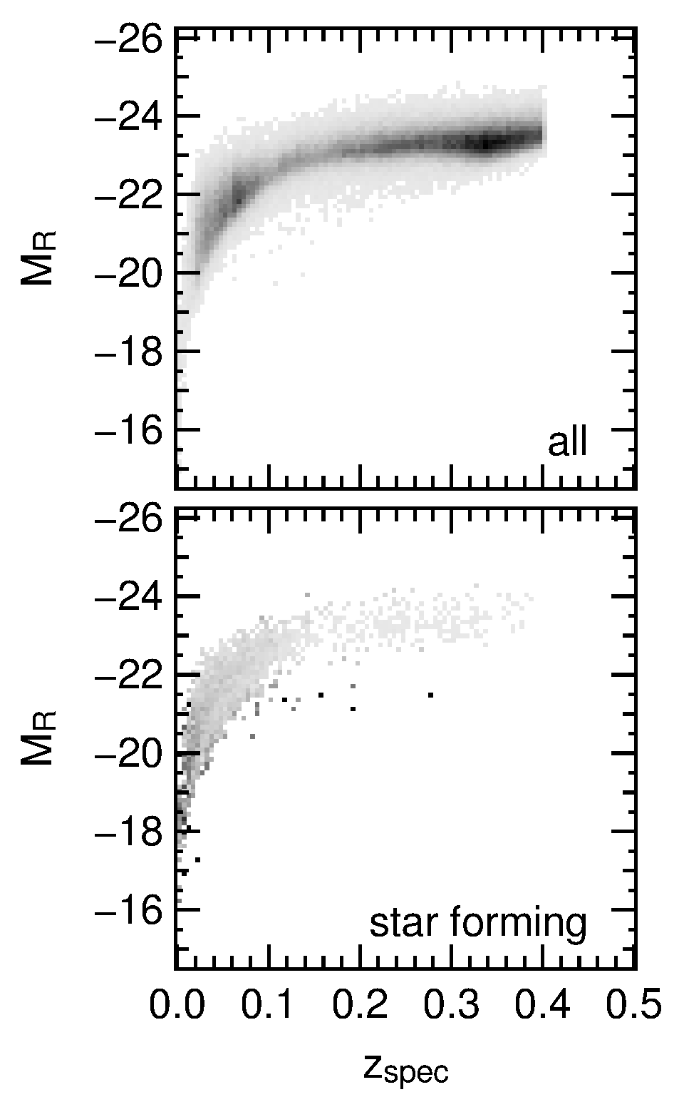
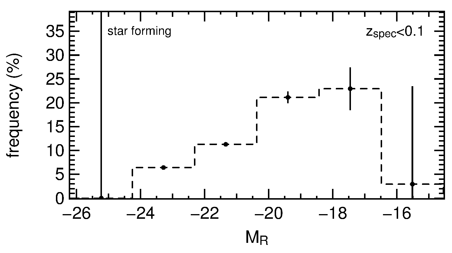
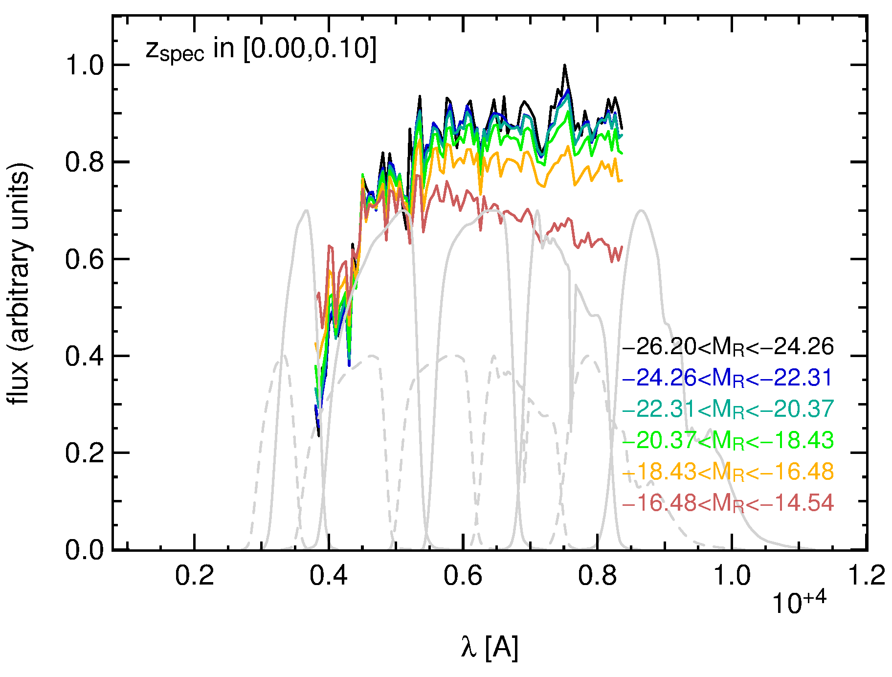
We want to compare our findings of the previous chapter to the observed spectra of SDSS LRGs. Therefore, we download the SDSS spectral subclassifications of our LRG sample that were produced by the SpecBS pipeline, where galaxies are further categorized by their emission lines. Galaxies that fulfill are tagged as “star forming”. If they furthermore have an equivalent width of equal or greater than , they are classified as “starburst”. In our LRG sample only objects fulfill the “starburst” criteria. In the following, we will refer to both tags (“starforming” and “starburst”) as star forming. Since the spectral wavelength coverage of SDSS is , the line drops out of the sample at . From the previously investigated objects, remain in the sample when we cut off LRGs that have . From these, show indications of star formation. The upper panel of Figure 16 shows the density of LRGs in the plane, and the lower panel displays the relative abundances of LRGs exhibiting star formation. Here, one can observe that the fraction of local star forming LRGs increases toward smaller luminosities. Additionally, we show in Figure 17 the percental fractions of star-forming LRGs for the same redshift-absolute band magnitude bins that we investigated in Section 7.2, Figures 13 and 14. The errors in the intermediate bins are Poissonian errors. The errors of the outer two luminosity bins, which do not contain as many objects, are Binomial with a confidence level of . In principle, the highest and lowest bins could be neglected, since they contain only and objects, respectively. Except for the region of faint galaxies (the lowest luminosity bin), the frequencies of star-forming LRGs shows an increase toward fainter magnitudes. This is in agreement with what we would expect from Figure 14, where we saw that the mean model SEDs for faint LRGs are bluer and show more star-forming activity, as well as with the results of the fit we performed in the last section. In addition to that we downloaded spectra for random subsamples of the objects with and stacked them. Thereby we weighted them by the best fit SED flux in the band as we did with the superposition of our models in Section 7.2. In each luminosity bin the spectra of a subsample containing objects (less, if the bin contains less objects) were superpositioned. We show the results in Figure 18, where we consider the added spectra in the rest frame wavelength range which is covered by SDSS for objects with . Comparing Figure 18 to Figure 14, we observe that the stacked SDSS spectra show a very similar behavior as the average best fitting SEDs that were inspected previously, supporting that our novel SEDs are able to describe the data of this population. At greater redshifts (), no faint galaxies are observable, and only () LRGs are classified as starforming. This region is therefore strongly dominated by objects that show no recent star formation. The variations we saw in Figure 15 are not caused by different fractions of star forming galaxies (which are anyhow of very low abundance), but result from aging only, which was also supported by the fit to BC03 models we performed in Section7.2. We also stacked spectra of objects from these bins in the same manner as above. Unfortunately, one cannot see the effect of a flatter NIR and declining UV flux at low compared to a declining NIR and increasing UV flux at high as clearly as in Figure 15, because the NIR part is only observable for objects with low , and the UV only for objects with high . However, the trends at low (i.e., flat NIR flux) and at high (increasing UV flux) are qualitatively there.
8. Summary
In this work we analyzed the colors as a function of redshift of a number of publicly available red model SEDs in the SDSS filter system and compared them to the colors of spectroscopic SDSS LRGs at redshifts from to . We found that no investigated model set can describe the , , , and colors of the data at all redshifts. Thus we created new red model SEDs for five redshift bins on the basis of the LRG photometry by fitting a superposition of a BC03 CSP model and a burst SED, while allowing for dust extinction of both components. We estimated photometric redshifts with the Bayesian template fitting code PhotoZ and a template set containing the created SEDs with according redshift and luminosity priors. The resulting catastrophic outlier rate is , whereas the scatter reads and for non-outliers. The overall bias reaches . We compared our results with photometric redshift estimates available in the SDSS database, both for the template fitting approach and for the neural networks. Our , , and are of the same order as the SDSS database template fitting values, although with a slightly higher catastrophic outlier rate. Nevertheless, the medium bias varies significantly less from with our template SEDs. The total values of our scatter, bias and outlier rates marginally differ from the SDSS ANN(CC2) photometric redshifts and are worse than the results of ANN(D1). However, the bias of ANN redshifts reaches higher values within some redshift ranges. We investigated the properties of the novel SEDs and demonstrated that they also describe the variety of GALEX NUV and FUV colors well. Performing an SED fit at the spectroscopic redshift of the LRGs, we observed that the flux weighted mean SEDs of local galaxies () vary notably as a function of luminosity, meaning that faint galaxies show increasing indications of ongoing star formation. The stacked spectra from the SDSS show a very similar behavior. Furthermore, we find that the fraction of star forming SDSS LRGs at increases with decreasing band luminosity. This is in agreement with our finding that the mean SED is bluer for faint local galaxies. We also observe a difference in the flux weighted mean SEDs as a function of , which is an effect of aging only and not due to recent star formation. In Appendices A and B we showed that BC03 models cover the data better than M09 and M11 in color space, which is why we favored the BC03 relative to the M09 and M11 model sets for the creation of our new SEDs. Finally, we also showed how our new template SED colors compare to the data in the , , , and planes. We would be happy to provide the photometric redshifts together with the rest frame magnitudes for the complete photometric LRG sample of SDSS on request.
References
- Abazajian et al. (2009) Abazajian, K. N., Adelman-McCarthy, J. K., Agüeros, M. A., et al. 2009, ApJS, 182, 543
- Arnouts et al. (1999) Arnouts, S., Cristiani, S., Moscardini, L., et al. 1999, MNRAS, 310, 540
- Babbedge et al. (2004) Babbedge, T. S. R., Rowan-Robinson, M., Gonzalez-Solares, E., et al. 2004, MNRAS, 353, 654
- Bender et al. (2001) Bender, R., Appenzeller, I., Böhm, A., et al. 2001, in Deep Fields, ed. S. Cristiani, A. Renzini, & R. E. Williams, 96
- Benítez (2000) Benítez, N. 2000, ApJ, 536, 571
- Benítez et al. (2004) Benítez, N., Ford, H., Bouwens, R., et al. 2004, ApJS, 150, 1
- Benítez et al. (2009) Benítez, N., Gaztañaga, E., Miquel, R., et al. 2009, ApJ, 691, 241
- Bolzonella et al. (2000) Bolzonella, M., Miralles, J.-M., & Pelló, R. 2000, A&A, 363, 476
- Brammer et al. (2008) Brammer, G. B., van Dokkum, P. G., & Coppi, P. 2008, ApJ, 686, 1503
- Brimioulle et al. (2008) Brimioulle, F., Lerchster, M., Seitz, S., Bender, R., & Snigula, J. 2008, ArXiv e-prints
- Brimioulle et al. (2013) Brimioulle, F., Seitz, S., Lerchster, M., Bender, R., & Snigula, J. 2013, ArXiv e-prints
- Bruzual & Charlot (1993) Bruzual, G., & Charlot, S. 1993, ApJ, 405, 538
- Bruzual & Charlot (2003) —. 2003, MNRAS, 344, 1000
- Calzetti et al. (2000) Calzetti, D., Armus, L., Bohlin, R. C., et al. 2000, ApJ, 533, 682
- Capak et al. (2007) Capak, P., Abraham, R. G., Ellis, R. S., et al. 2007, ApJS, 172, 284
- Chabrier (2003) Chabrier, G. 2003, PASP, 115, 763
- Chuter et al. (2011) Chuter, R. W., Almaini, O., Hartley, W. G., et al. 2011, MNRAS, 413, 1678
- Coleman et al. (1980) Coleman, G. D., Wu, C., & Weedman, D. W. 1980, ApJS, 43, 393
- Csabai et al. (2000) Csabai, I., Connolly, A. J., Szalay, A. S., & Budavári, T. 2000, AJ, 119, 69
- Csabai et al. (2003) Csabai, I., Budavári, T., Connolly, A. J., et al. 2003, AJ, 125, 580
- Drory et al. (2004) Drory, N., Bender, R., & Hopp, U. 2004, ApJ, 616, L103
- Drory et al. (2001) Drory, N., Feulner, G., Bender, R., et al. 2001, MNRAS, 325, 550
- Eisenstein et al. (2001) Eisenstein, D. J., Annis, J., Gunn, J. E., et al. 2001, AJ, 122, 2267
- Eisenstein et al. (2003) Eisenstein, D. J., Hogg, D. W., Fukugita, M., et al. 2003, ApJ, 585, 694
- Feldmann et al. (2006) Feldmann, R., Carollo, C. M., Porciani, C., et al. 2006, MNRAS, 372, 565
- Feulner et al. (2005) Feulner, G., Gabasch, A., Salvato, M., et al. 2005, ApJ, 633, L9
- Gabasch et al. (2008) Gabasch, A., Goranova, Y., Hopp, U., Noll, S., & Pannella, M. 2008, MNRAS, 383, 1319
- Gabasch et al. (2004) Gabasch, A., Bender, R., Seitz, S., et al. 2004, A&A, 421, 41
- Gustafsson et al. (2008) Gustafsson, B., Edvardsson, B., Eriksson, K., et al. 2008, A&A, 486, 951
- Ilbert et al. (2006) Ilbert, O., Arnouts, S., McCracken, H. J., et al. 2006, A&A, 457, 841
- Ilbert et al. (2009) Ilbert, O., Capak, P., Salvato, M., et al. 2009, ApJ, 690, 1236
- Kroupa (2001) Kroupa, P. 2001, MNRAS, 322, 231
- Le Borgne & Rocca-Volmerange (2002) Le Borgne, D., & Rocca-Volmerange, B. 2002, A&A, 386, 446
- Ma et al. (2006) Ma, Z., Hu, W., & Huterer, D. 2006, ApJ, 636, 21
- Madau (1995) Madau, P. 1995, ApJ, 441, 18
- Mancone & Gonzalez (2012) Mancone, C. L., & Gonzalez, A. H. 2012, PASP, 124, 606
- Mannucci et al. (2001) Mannucci, F., Basile, F., Poggianti, B. M., et al. 2001, MNRAS, 326, 745
- Maraston & Strömbäck (2011) Maraston, C., & Strömbäck, G. 2011, MNRAS, 418, 2785
- Maraston et al. (2009) Maraston, C., Strömbäck, G., Thomas, D., Wake, D. A., & Nichol, R. C. 2009, MNRAS, 394, L107
- Nakajima et al. (2012) Nakajima, R., Mandelbaum, R., Seljak, U., et al. 2012, MNRAS, 420, 3240
- Oke & Gunn (1983) Oke, J. B., & Gunn, J. E. 1983, ApJ, 266, 713
- Oyaizu et al. (2008) Oyaizu, H., Lima, M., Cunha, C. E., et al. 2008, ApJ, 674, 768
- Padmanabhan et al. (2005) Padmanabhan, N., Budavári, T., Schlegel, D. J., et al. 2005, MNRAS, 359, 237
- Pickles (1998) Pickles, A. J. 1998, PASP, 110, 863
- Ree et al. (2012) Ree, C. H., Jeong, H., Oh, K., et al. 2012, ApJ, 744, L10
- Roig et al. (2009) Roig, D., Verde, L., Miralda-Escudé, J., Jimenez, R., & Peña-Garay, C. 2009, J. Cosmology Astropart. Phys, 4, 8
- Saglia et al. (2012) Saglia, R. P., Tonry, J. L., Bender, R., et al. 2012, ApJ, 746, 128
- Sánchez et al. (2011) Sánchez, E., Carnero, A., García-Bellido, J., et al. 2011, MNRAS, 411, 277
- Sánchez-Blázquez et al. (2006) Sánchez-Blázquez, P., Peletier, R. F., Jiménez-Vicente, J., et al. 2006, MNRAS, 371, 703
- Schawinski et al. (2007) Schawinski, K., Kaviraj, S., Khochfar, S., et al. 2007, ApJS, 173, 512
- Schlegel et al. (1998) Schlegel, D. J., Finkbeiner, D. P., & Davis, M. 1998, ApJ, 500, 525
- Schneider et al. (1983) Schneider, D. P., Gunn, J. E., & Hoessel, J. G. 1983, ApJ, 264, 337
- Silva et al. (1998) Silva, L., Granato, G. L., Bressan, A., & Danese, L. 1998, ApJ, 509, 103
- York et al. (2000) York, D. G., Adelman, J., Anderson, Jr., J. E., et al. 2000, AJ, 120, 1579
Appendix A SED Fitting Results with Different Model Sets
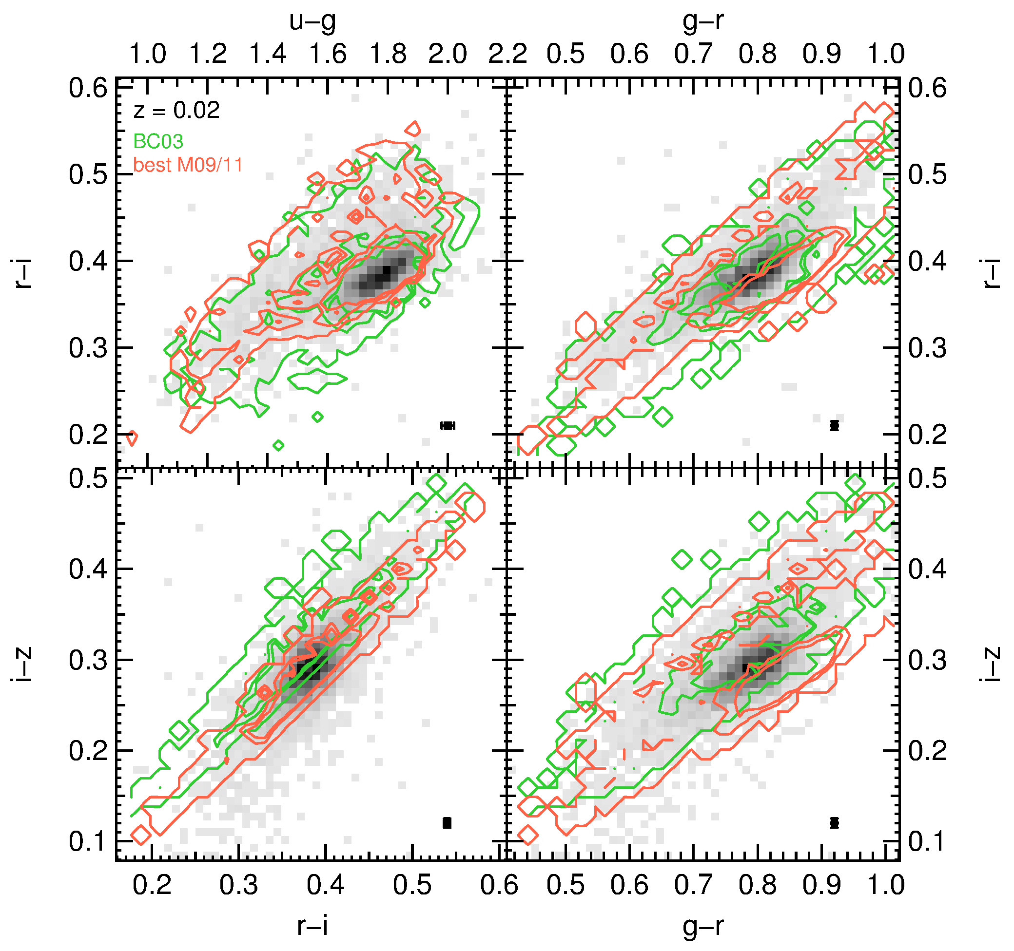
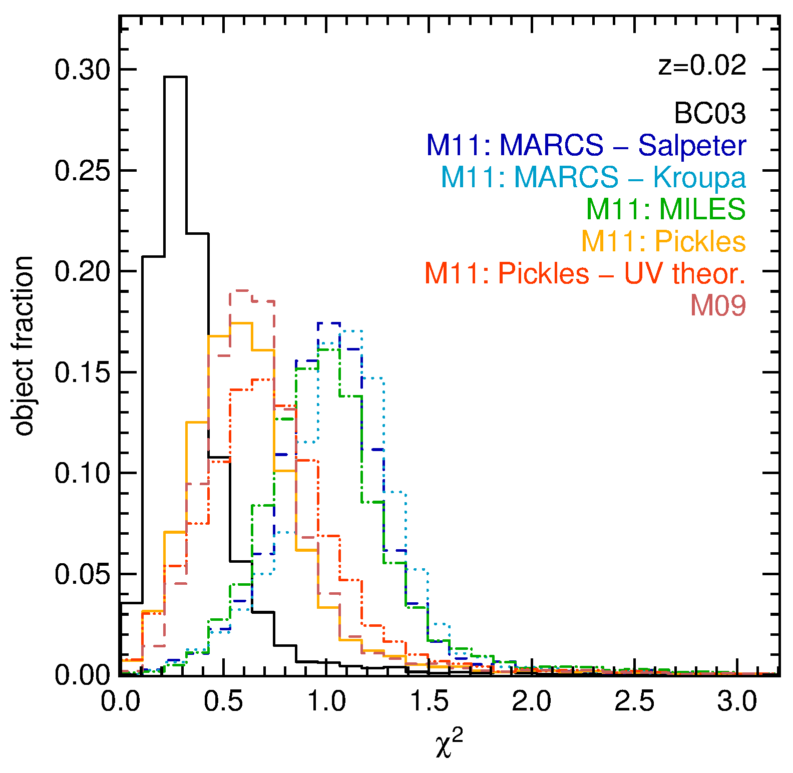
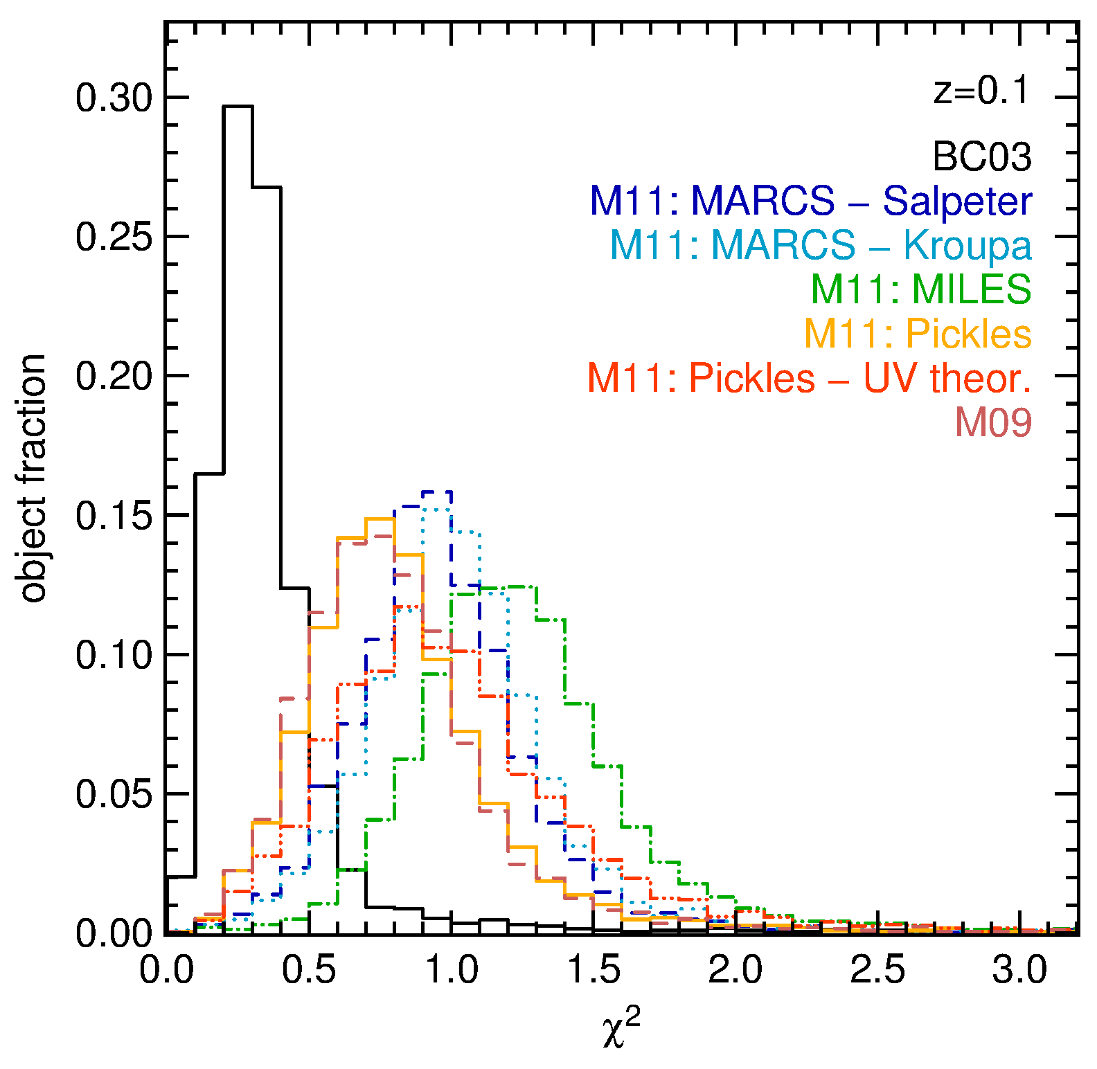
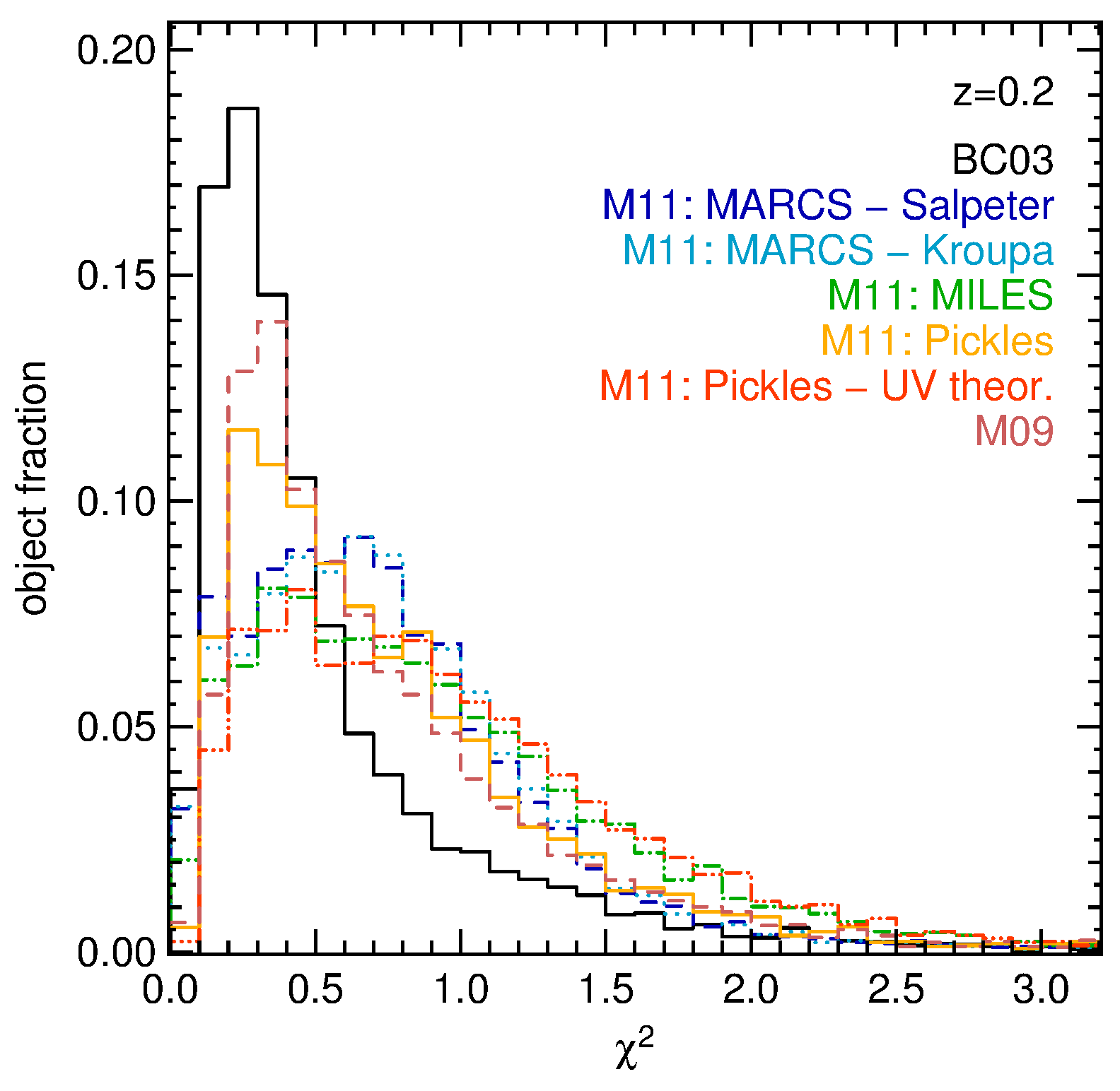
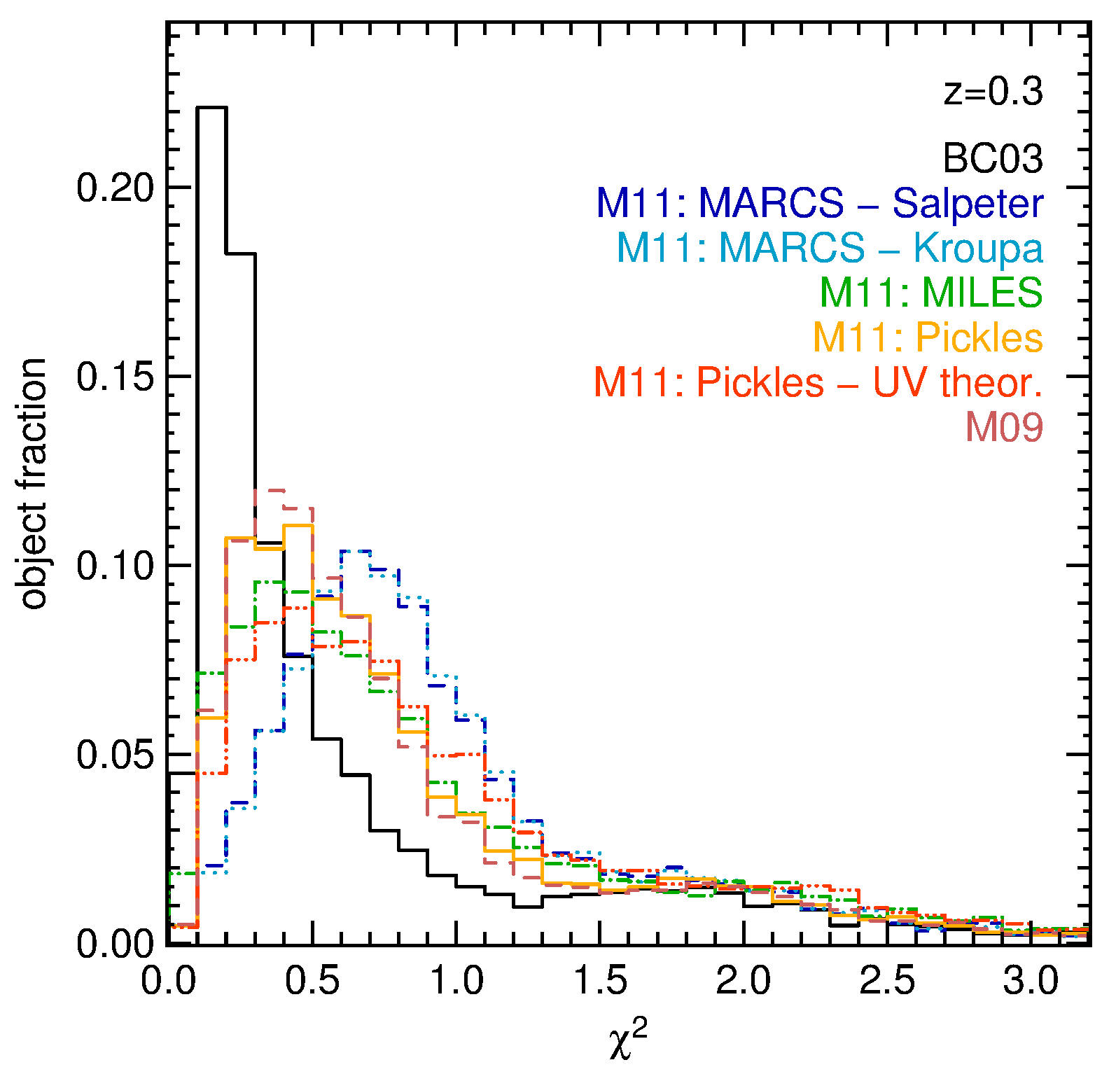
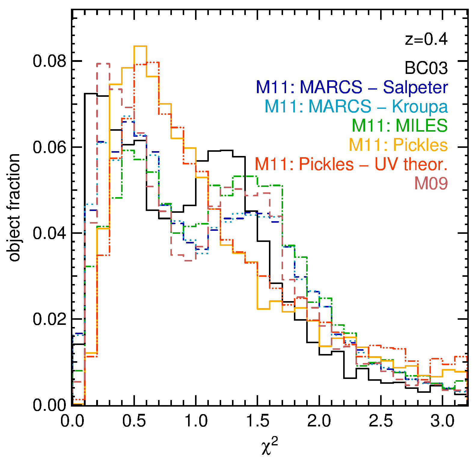
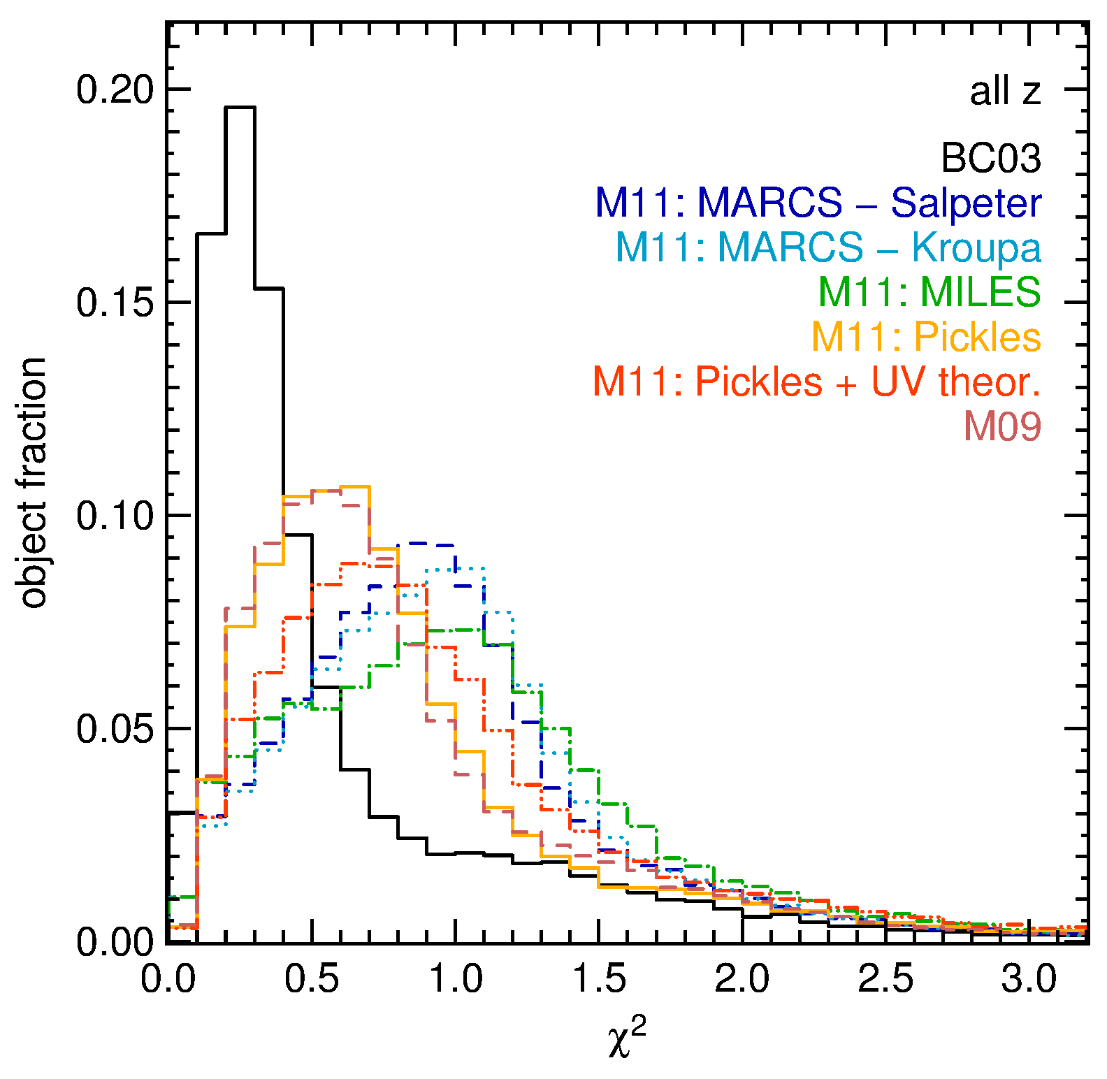
In Section 4 we created templates by fitting model SEDs to the photometry of the SDSS LRGs in order to produce SEDs matching the colors of the data. Here we want to show the fitting results and how well the models are able to cover the observed colors. In Figures 2 and 5 we saw that both the BC03 and the M09 model SEDs can represent the LRG data, at least for a large part of the investigated redshift range. Both sets have a large variety of ages (plus -folding timescales and metallicities in the case of BC03 models), thus they offer the perspective to provide a well matching model for each redshift. In addition to that, Maraston & Strömbäck (2011, M11) provide a large variety of single stellar populations (SSPs) created from different stellar libraries and with varying metallicities and ages. The M11 models are promising candidates to represent the LRG data in terms of colors, wherefore we analyzed them in this regard and compared to the results with BC03 models. We could only use those M11 model SEDs that are provided for a wavelength range sufficiently large to cover all SDSS filters at all LRG redshifts. These are two flux-calibrated empirical stellar spectral libraries, Pickles (Pickles, 1998) and MILES (Sánchez-Blázquez et al., 2006), and the theoretically derived MARCS (Gustafsson et al., 2008) library. The Pickles models have solar metallicity, either an IMF of Chabrier (2003) or Salpeter, and were extended in the near-IR by M11. A version with a theoretical UV part was additionally created by M11. The MILES SSPs in question were extended in the near-IR and UV, have a revised IR slope, and solar metallicity. The MARCS models have metallicities of , and , and IMFs of Salpeter and Kroupa (2001) respectively… A more thorough description of the SSPs as well as the SEDs can be found in M11 and at http://www.icg.port.ac.uk/~maraston/M11/. These models are a subset of all M11 covering a wavelength range wide enough for photometric redshift estimation. We produced CSPs from the selected M11 models with the software EzGal777http://www.baryons.org/ezgal/ (Mancone & Gonzalez, 2012). We apply exponential SFRs and the same -folding timescales that were used with BC03 (Section 3.2.2). The whole range of available ages, IMFs, and metallicities were exploited where possible in order to cover the greatest variety within the resulting SEDs. These CSPs were then fitted to the photometry in the same way as the BC03 CSPs in Section 4 (i.e., superposed by a burst model and with additional extinction) for each stellar library and IMF separately. The same was also done with M09 models. The SED fitting results for the different redshift bins and color spaces of M09/11 are shown together with those of the BC03 models in Figure 19. From the M09/11 models in all cases the one with the smallest result is chosen for the plot. The upper left panel of Figure 19 () shows that the BC03 models cover the LRG colors better in this range, with the exception of , where M09/M11 account for the lower right part that is not covered by BC03. Furthermore, the BC03 color contours trace the LRG distribution better than M09/11 in and . In the upper right and middle left panel the colors are shown for the redshift bins at , and . Both model sets perform similarly well, except for , where M09/11 produces a slightly wider spread in . Apart from that, the BC03 contours follow well the density of the LRGs in the color spaces and . At the M09/11 models outperform BC03 in , whereas both describe the data colors similarly in the other spaces (middle right panel). Here, the M09/11 SEDs produce two peaks in which cannot be observed for the LRGs. Finally, the lower panel of Figure 19 shows the redshift bin around , where M09/M11 still produce a wider spread in , but are not able to match the bluer part of the LRG’s color. In addition to that, neither BC03 nor M09/11 models cover the bluer part of the color. In Section 4.2 we already mentioned that the spread in the colors of the data cannot be completely accounted for by the photometric errors in this redshift range. The reason for the spread must thus be of physical origin. Unfortunately, not the whole range of of LRGs at can be fitted by the investigated models sets while simultaneously matching the and colors (where the latter has smaller errors than ). This is a feature of BC03 and M09/11 models, and the reason why we could not create SEDs with bluer in Section 4. The distributions of the results of the fitting to the various model sets are shown in Figure 20. Each analyzed bin is displayed in a different panel, whereas the distributions for all redshift intervals combined is shown in the lower right panel. BC03 outperforms the other models (M09 and M11), regarding the values, in every redshift slice except for , where the M11 Pickles models fit the LRGs better, but only marginally. We would like to add that the M11 Pickles models fit the data best compared to the other M09/M11 SEDs, and outperform the Pickles models with a theoretical UV-part of the spectrum for each fitted object. Finally, the lower right panel of Figure 20 shows that the values are best also for all bins combined, as expected from the previous results. Following these results, and because of the previous analysis of the colors of the produced SEDs, we adopted the BC03 models for the creation of photo- template SEDs.
Appendix B Color–Color Relations of the New Models
Here we present the color–color relations of our models and the LRG data. Figures 6, and 21–25 show the colors of the best fitting SED models, the preselected models, and the selected models after the removal of redundant SEDs in comparison to the LRG data itself in the , , , and color spaces. We display the LRGs with band errors below the median and those with errors above with different colors to visualize the difference in the populated loci within the space, which becomes evident at (Figure 24, upper panel) and (Figure 25, upper panel). The grids we imposed on the plane within which we selected templates (see Section 4.2) are displayed in the upper left panels of Figures 6 , and 22–25, whereas the color boundaries in and are drawn in the lower panel of Figure 6, in Figure 21 and in the lower left and in the right panels of Figures 22–25. In order to account for objects with peculiar colors which lie outside the boundaries as well, we select additional SEDs by eye and confirm that they yield a photometric redshift bias lower than 0.01, when used as single template for the subcatalog from the same range. If they do not meet that requirement, we chose the SED of another object from the color neighborhood of the first one, test for the bias, and so on until we find a model from that color locus which creates only a small -bias. Bright cluster galaxies (BCGs) with very low UV-excess (i.e., in the lower part of the UV red sequence; see Section 7.1, Figure 12) at are not matched by the models already selected for that range. But we find that two SEDs originating from are able to cover the considered region. Therefore, we add these templates to , i.e., we assign the same redshift priors as for models in addition to their former priors (see Section 2), thereby covering the lower UV red sequence. The colors of these two models are shown by yellow triangles in Figure 22.
