Unstable Galaxy Models

Zhiyu Wang School of Mathematical Sciences
Peking University
Beijing, 100871, P. R. China
Yan Guo Division of Applied Mathematics
Brown University
Providence, RI 02912, USA
Zhiwu Lin School of Mathematics
Georgia Institute of Technology
Atlanta, GA 30332, USA
 and  Pingwen Zhang School of Mathematical Sciences
Peking University
Beijing, 100871, P. R. China
Abstract.

The dynamics of collisionless galaxy can be described by the Vlasov-Poisson system. By the Jean’s theorem, all the spherically symmetric steady galaxy models are given by a distribution of Φ(E,L)Φ𝐸𝐿\Phi(E,L), where E𝐸E is the particle energy and L𝐿L the angular momentum. In a celebrated Doremus-Feix-Baumann Theorem [7], the galaxy model Φ(E,L)Φ𝐸𝐿\Phi(E,L) is stable if the distribution ΦΦ\Phi is monotonically decreasing with respect to the particle energy E.𝐸E. On the other hand, the stability of Φ(E,L)Φ𝐸𝐿\Phi(E,L) remains largely open otherwise. Based on a recent abstract instability criterion of Guo-Lin [11], we constuct examples of unstable galaxy models of f(E,L)𝑓𝐸𝐿f(E,L) and f(E)𝑓𝐸f\left(E\right)\ in which f𝑓f fails to be monotone in E.𝐸E.

1. Introduction

A galaxy is an ensemble of billions of stars, which interact by the gravitational field they create collectively. For galaxies, the collisional relaxation time is much longer than the age of the universe ([6]). The collisions can therefore be ignored and the galactic dynamics is well described by the Vlasov - Poisson system (collisionless Boltzmann equation)

(1) tf+vxfxUfvf=0, ΔUf=4π𝐑3f(t,x,v)𝑑v,formulae-sequencesubscript𝑡𝑓𝑣subscript𝑥𝑓subscript𝑥subscript𝑈𝑓subscript𝑣𝑓0 Δsubscript𝑈𝑓4𝜋subscriptsuperscript𝐑3𝑓𝑡𝑥𝑣differential-d𝑣\partial_{t}f+v\cdot\nabla_{x}f-\nabla_{x}U_{f}\cdot\nabla_{v}f=0,\text{ \ \ \ \ \ }\Delta U_{f}=4\pi\int_{\mathbf{R}^{3}}f(t,x,v)dv,

where (x,v)3×3𝑥𝑣superscript3superscript3\left(x,v\right)\in\mathbb{R}^{3}\times\mathbb{R}^{3}, f(t,x,v)𝑓𝑡𝑥𝑣f(t,x,v) is the distribution function and Uf(t,x)subscript𝑈𝑓𝑡𝑥U_{f}\left(t,x\right) is its self-consistent gravitational potential. The Vlasov-Poisson system can also be used to describe the dynamics of globular clusters over their period of orbital revolutions ([9]). One of the central questions in such galactic problems, which has attracted considerable attention in the astrophysics literature, of [5], [6], [9], [17] and the references there, is to determine dynamical stability of steady galaxy models. Stability study can be used to test a proposed configuration as a model for a real stellar system. On the other hand, instabilities of steady galaxy models can be used to explain some of the striking irregularities of galaxies, such as spiral arms as arising from the instability of an initially featureless galaxy disk ([5]), ([18]).

In this article, we consider stability of spherical galaxies, which are the simplest elliptical galaxy models. Though most elliptical galaxies are known to be non-spherical, the study of instability and dynamical evolution of spherical galaxies could be useful to understand more complicated and practical galaxy models. By Jeans’s Theorem, a steady spherical galaxy is of the form f(x,v)μ(E,L)𝑓𝑥𝑣𝜇𝐸𝐿f(x,v)\equiv\mu(E,L), where the particle energy and total momentum are E=12|v|2+U(x),L=|x×v|,formulae-sequence𝐸12superscript𝑣2𝑈𝑥𝐿𝑥𝑣E=\frac{1}{2}|v|^{2}+U(x),\ L=\left|x\times v\right|, and Uμ(x)=U(|x|)subscript𝑈𝜇𝑥𝑈𝑥U_{\mu}(x)=U\left(\left|x\right|\right) satisfies the self-consistent nonlinear Poisson equation

ΔU=4π𝐑3μ(E,L)𝑑vΔ𝑈4𝜋subscriptsuperscript𝐑3𝜇𝐸𝐿differential-d𝑣\Delta U=4\pi\int_{\mathbf{R}^{3}}\mu(E,L)dv

The isotropic models take the form f(x,v)μ(E).𝑓𝑥𝑣𝜇𝐸f(x,v)\equiv\mu(E). The case when μ(E)<0superscript𝜇𝐸0\mu^{\prime}(E)<0 (on the support of μ(E)𝜇𝐸\mu(E))  has been widely studied and these models are known to be stable ([1], [2], [7], [2], [8], [20], [14], [19], [13]). To understand such a stability, we expand the well-known Casimir-Energy functional (as a Liapunov functional)

(2) Q(f)+12|v|2f18π|xU|2𝑄𝑓12superscript𝑣2𝑓18𝜋superscriptsubscript𝑥𝑈2\mathcal{H}\equiv\int\int Q(f)+\frac{1}{2}\int\int|v|^{2}f-\frac{1}{8\pi}\int|\nabla_{x}U|^{2}

which is conserved for all time with

(3) Q(μ(E))Esuperscript𝑄𝜇𝐸𝐸Q^{\prime}(\mu(E))\equiv-E

(((this is possible only if μ<0!superscript𝜇0\mu^{\prime}<0!). Upon using Taylor expansion around a steady galaxy model of [f(E,L),U],𝑓𝐸𝐿𝑈[f(E,L),U], the first order variation vanishes due to the choice of (3), and the second order variation takes the form of

(4) f′′[g,g]12f>0g2f(E)18π|xUg|2.superscriptsubscript𝑓′′𝑔𝑔12subscript𝑓0superscript𝑔2superscript𝑓𝐸18𝜋superscriptsubscript𝑥subscript𝑈𝑔2\mathcal{H}_{f}^{\prime\prime}[g,g]\equiv\frac{1}{2}\int\int_{f>0}\frac{g^{2}}{-f^{\prime}(E)}-\frac{1}{8\pi}\int|\nabla_{x}U_{g}|^{2}.

The remarkable feature for stability lies in the fact that μ′′[g,g]>0superscriptsubscript𝜇′′𝑔𝑔0\mathcal{H}_{\mu}^{\prime\prime}[g,g]>0 if μ<0superscript𝜇0\mu^{\prime}<0 ([1], [2], [7], [14]). This crucial observation leads to the conclusion that galaxy models with monotonically decreasing energy μ<0superscript𝜇0\mu^{\prime}<0 are linearly stable. On the other hand, for the case μ𝜇\mu is not monotone in E𝐸E, (3) breaks down, and μ′′superscriptsubscript𝜇′′\mathcal{H}_{\mu}^{\prime\prime} is not well-defined, which indicates possible formation of instability. It is important to note that a negative direction of the quadratic form f′′[g,g]<0superscriptsubscript𝑓′′𝑔𝑔0\mathcal{H}_{f}^{\prime\prime}[g,g]<0 does not imply instability. In [12], an oscillatory instability was found for certain generalized polytropes f(E,L)=f0L2m(E0E)n32𝑓𝐸𝐿subscript𝑓0superscript𝐿2𝑚superscriptsubscript𝐸0𝐸𝑛32f\left(E,L\right)=f_{0}L^{-2m}\left(E_{0}-E\right)^{n-\frac{3}{2}} with n<32,m<0,formulae-sequence𝑛32𝑚0n<\frac{3}{2},m<0,\ by using N-body code. This instability was later reanalyzed by more sophisticated N-body code in [3]. Despite progresses made over the years (e.g., [3], [10], [17], [18]), no explicit example of isotropic galaxy model μ(E)𝜇𝐸\mu(E) are known to be unstable.

The difficulty of finding instability lies in the complexity of the linearized Vlasov-Poisson system around a spatially non-homogeneous μ(E,L)::𝜇𝐸𝐿absent\mu(E,L):

(5) tg+vxgxUgvμxUvg=0,ΔUg=4π𝐑3g(x,v)𝑑vformulae-sequencesubscript𝑡𝑔𝑣subscript𝑥𝑔subscript𝑥subscript𝑈𝑔subscript𝑣𝜇subscript𝑥𝑈subscript𝑣𝑔0Δsubscript𝑈𝑔4𝜋subscriptsuperscript𝐑3𝑔𝑥𝑣differential-d𝑣\partial_{t}g+v\cdot\nabla_{x}g-\nabla_{x}U_{g}\cdot\nabla_{v}\mu-\nabla_{x}U\cdot\nabla_{v}g=0,\ \ \Delta U_{g}=4\pi\int_{\mathbf{R}^{3}}g(x,v)dv

for which the construction for dispersion relation for a growing mode is mathematically very challenging. In a recent paper ([11]), a sufficient condition was derived rigorously as follows:

Theorem 1.

Let [f(E,L),U]𝑓𝐸𝐿𝑈[f(E,L),U] be a steady galaxy model. Assume that f(E,L)𝑓𝐸𝐿f(E,L) has a compact support in x𝑥x and v,𝑣v, and μsuperscript𝜇\mu^{\prime} is bounded. Define auxiliary quadratic form for a spherically symmetric function ϕ(|x|)italic-ϕ𝑥\phi(|x|) as

(6) [A0ϕ,ϕ]𝐑3|ϕ|2𝑑x+32π3f(E,L)r1(E,L)r2(E,L)(ϕϕ¯)22LdrdEdL2(EU(r)L2/2r2),subscript𝐴0italic-ϕitalic-ϕsubscriptsuperscript𝐑3superscriptitalic-ϕ2differential-d𝑥32superscript𝜋3superscript𝑓𝐸𝐿superscriptsubscriptsubscript𝑟1𝐸𝐿subscript𝑟2𝐸𝐿superscriptitalic-ϕ¯italic-ϕ22𝐿𝑑𝑟𝑑𝐸𝑑𝐿2𝐸𝑈𝑟superscript𝐿22superscript𝑟2[A_{0}\phi,\phi]\equiv\int_{\mathbf{R}^{3}}|\nabla\phi|^{2}dx+32\pi^{3}\int f^{\prime}(E,L)\int_{r_{1}(E,L)}^{r_{2}(E,L)}\left(\phi-\bar{\phi}\right)^{2}\frac{2LdrdEdL}{\sqrt{2(E-U(r)-L^{2}/2r^{2})}},

where r1(E,L)subscript𝑟1𝐸𝐿r_{1}(E,L) and r2(E,L)subscript𝑟2𝐸𝐿r_{2}(E,L) are two distinct roots to the equation

(7) EU(r)L2/2r2=0𝐸𝑈𝑟superscript𝐿22superscript𝑟20E-U(r)-L^{2}/2r^{2}=0

and the average ϕ¯¯italic-ϕ\bar{\phi} is defined as

ϕ¯(E,L)=r1(E,L)r2(E,L)ϕ(r)dr2(EU0(r)L2/2r2)r1(E,L)r2(E,L)dr2(EU0(r)L2/2r2).¯italic-ϕ𝐸𝐿superscriptsubscriptsubscript𝑟1𝐸𝐿subscript𝑟2𝐸𝐿italic-ϕ𝑟𝑑𝑟2𝐸subscript𝑈0𝑟superscript𝐿22superscript𝑟2superscriptsubscriptsubscript𝑟1𝐸𝐿subscript𝑟2𝐸𝐿𝑑𝑟2𝐸subscript𝑈0𝑟superscript𝐿22superscript𝑟2\bar{\phi}(E,L)=\frac{\int_{r_{1}(E,L)}^{r_{2}(E,L)}\frac{\phi(r)dr}{\sqrt{2(E-U_{0}(r)-L^{2}/2r^{2})}}}{\int_{r_{1}(E,L)}^{r_{2}(E,L)}\frac{dr}{\sqrt{2(E-U_{0}(r)-L^{2}/2r^{2})}}}.

If there exists ϕ(|x|)italic-ϕ𝑥\phi(|x|) such that [A0ϕ,ϕ]<0subscript𝐴0italic-ϕitalic-ϕ0[A_{0}\phi,\phi]<0, then there exists an exponentially growing mode to the linearized Vlasov-Poisson system (5).

The quadratic form [A0ϕ,ϕ]subscript𝐴0italic-ϕitalic-ϕ[A_{0}\phi,\phi] in the above instability criterion involves delicate integrals along particle paths. The purpose of the current paper is to use numerical computations to construct two explicit examples of galaxy models for which a test function ϕitalic-ϕ\phi\ satisfying [A0ϕ,ϕ]<0subscript𝐴0italic-ϕitalic-ϕ0[A_{0}\phi,\phi]<0 exists. This ensures their radial instability by Guo-Lin’s Theorem 1. The first example is an anisotropic model with radial instability. There are two differences to the oscillatory instability found in [12] and [3]: here the distribution function is non-singular and the instability is non-oscillatory. The second example is a non-singular isotropic model with radial instability. To our knowledge, this provides the first example of unstable isotropic model.

Even though the galaxy models studied here are not actual ones observed, our results demonstrates how to apply Guo-Lin’s Theorem 1 to detect possible instability for a given galaxy model. It is our hope to foster interactions between mathematical and astronomical communities and to advance the study of instability of real galaxy models.

2. Examples of Unstable galaxy models

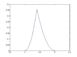
Example 1. Unstable Galaxy Model Depending on E𝐸E~{}and L.𝐿L. We define the distribution function f0(E,L)=μ(E)L4subscript𝑓0𝐸𝐿𝜇𝐸superscript𝐿4f_{0}\left(E,L\right)=\mu(E)L^{4} where

(8) μ(E)={0E<42.25(E4)24E4.4(5E)24.4E50E>5𝜇𝐸cases0𝐸42.25superscript𝐸424𝐸4.4superscript5𝐸24.4𝐸50𝐸5\mu(E)=\left\{\begin{array}[c]{l}0\quad E<4\\ 2.25(E-4)^{2}\quad 4\leq E\leq 4.4\\ (5-E)^{2}\quad 4.4\leq E\leq 5\\ 0\quad E>5\end{array}\right.

The graph of μ(E)𝜇𝐸\mu(E) is showed in Figure 1 below.

Refer to caption
Figure 1. μ(E)𝜇𝐸\mu(E)

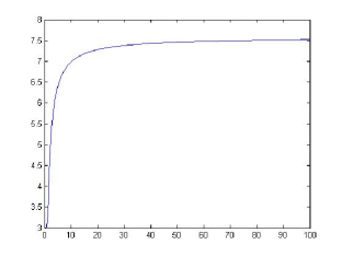
Choosing U(0)=3𝑈03U(0)=3, we numerically calculate U(r)𝑈𝑟U(r), and the graph of U(r)𝑈𝑟U(r) is showed in Figure 2.

Refer to caption
Figure 2. U(r)𝑈𝑟U(r)

By choosing the test function ϕ=er,italic-ϕsuperscript𝑒𝑟\phi=e^{-r}, then numerical computation below shows

[A0ϕ,ϕ]<π45<0,subscript𝐴0italic-ϕitalic-ϕ𝜋450[A_{0}\phi,\phi]<\pi-45<0,

and hence f0subscript𝑓0f_{0} is unstable by Theorem 1.

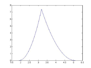
Example 2. Unstable Galaxy Model Depending Only on E.𝐸E. Let f0(E)=μ(E)subscript𝑓0𝐸𝜇𝐸f_{0}(E)=\mu(E), where

(9) μ(E)={0E<aC1t1k(Ea)kaEE1C1(E0E)kE1EE00E>E0𝜇𝐸cases0𝐸𝑎subscript𝐶1superscriptsubscript𝑡1𝑘superscript𝐸𝑎𝑘𝑎𝐸subscript𝐸1subscript𝐶1superscriptsubscript𝐸0𝐸𝑘subscript𝐸1𝐸subscript𝐸00𝐸subscript𝐸0\mu(E)=\left\{\begin{array}[c]{l}0\quad E<a\\ C_{1}t_{1}^{k}(E-a)^{k}\quad a\leq E\leq E_{1}\\ C_{1}(E_{0}-E)^{k}\quad E_{1}\leq E\leq E_{0}\\ 0\quad E>E_{0}\end{array}\right.

We choose

C1=2,E0=5.1,a=1.9,k=2.01,t1=1.5.formulae-sequencesubscript𝐶12formulae-sequencesubscript𝐸05.1formulae-sequence𝑎1.9formulae-sequence𝑘2.01subscript𝑡11.5C_{1}=2\newline ,\ E_{0}=5.1,\ \newline a=1.9\newline ,\ k=2.01\newline ,\ t_{1}=1.5.

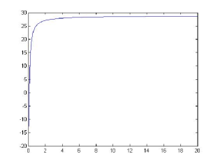
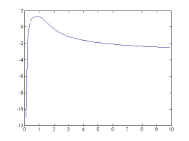
Choose U0=15.1subscript𝑈015.1U_{0}=-15.1, the graphs of μ(E)𝜇𝐸\mu(E) and U𝑈U are shown in Figures 3 and 4.

Refer to caption
Figure 3. μ(E)𝜇𝐸\mu(E)
Refer to caption
Figure 4. U(r)𝑈𝑟U(r)

We choose the test function

ϕ=v1er+v2e12r+v3e13r+v4e2r+v5e3r+v6e4r+v7e5r,italic-ϕsubscript𝑣1superscript𝑒𝑟subscript𝑣2superscript𝑒12𝑟subscript𝑣3superscript𝑒13𝑟subscript𝑣4superscript𝑒2𝑟subscript𝑣5superscript𝑒3𝑟subscript𝑣6superscript𝑒4𝑟subscript𝑣7superscript𝑒5𝑟\phi=v_{1}e^{-r}+v_{2}e^{-\frac{1}{2}r}+v_{3}e^{-\frac{1}{3}r}+v_{4}e^{-2r}+v_{5}e^{-3r}+v_{6}e^{-4r}+v_{7}e^{-5r},

with v1,v2,v7subscript𝑣1subscript𝑣2subscript𝑣7v_{1},v_{2},...v_{7} given by (16). Then [A0ϕ,ϕ]=24. 016<0,subscript𝐴0italic-ϕitalic-ϕ24.0160[A_{0}\phi,\phi]=-24.\,\allowbreak 016<0, and instability of the profile (9) follows from Theorem 1.

3. Numerical implementation

3.1. Numerical computation for Example 1

By the results in [21], for a steady state with f0(E,L)=μ(E)L2lsubscript𝑓0𝐸𝐿𝜇𝐸superscript𝐿2𝑙f_{0}\left(E,L\right)=\mu\left(E\right)L^{2l}\ of Vlasov-Poisson system, the steady potential U(r)𝑈𝑟U\left(r\right) satisfies the equation

(10) U(r)=2l+7/2π2cl,1/2r20rs2l+2gl+1/2(U(s))𝑑s,r>0formulae-sequencesuperscript𝑈𝑟superscript2𝑙72superscript𝜋2subscript𝑐𝑙12superscript𝑟2superscriptsubscript0𝑟superscript𝑠2𝑙2subscript𝑔𝑙12𝑈𝑠differential-d𝑠𝑟0U^{\prime}(r)=\frac{2^{l+7/2}\pi^{2}c_{l,-1/2}}{r^{2}}\int_{0}^{r}s^{2l+2}g_{l+1/2}(U(s))ds,\quad r>0

with gm(u)=uμ(E)(Eu)m𝑑E,u(,)formulae-sequencesubscript𝑔𝑚𝑢superscriptsubscript𝑢𝜇𝐸superscript𝐸𝑢𝑚differential-d𝐸𝑢g_{m}(u)=\int_{u}^{\infty}\mu(E)(E-u)^{m}dE,\quad u\in(-\infty,\infty),    and

ca,b=01sa(1s)b𝑑s=Γ(a+1)Γ(b+1)Γ(a+b+2),a>1,b>1,formulae-sequencesubscript𝑐𝑎𝑏superscriptsubscript01superscript𝑠𝑎superscript1𝑠𝑏differential-d𝑠Γ𝑎1Γ𝑏1Γ𝑎𝑏2formulae-sequence𝑎1𝑏1c_{a,b}=\int_{0}^{1}s^{a}(1-s)^{b}ds=\frac{\Gamma(a+1)\Gamma(b+1)}{\Gamma(a+b+2)},\ \ a>-1,b>-1,

where ΓΓ\Gamma denotes the gamma function. The boundary condition is limrU(r)=0subscript𝑟𝑈𝑟0\lim_{r\rightarrow\infty}U(r)=0.

The computation of finding ϕitalic-ϕ\phi with [A0ϕ,ϕ]<0subscript𝐴0italic-ϕitalic-ϕ0[A_{0}\phi,\phi]<0\ is carried out in the following steps.

Step 1. Computation of potential U.𝑈U. For Example 1, f0(E,L)=μ(E)L4subscript𝑓0𝐸𝐿𝜇𝐸superscript𝐿4f_{0}\left(E,L\right)=\mu\left(E\right)L^{4} where μ(E)𝜇𝐸\mu\left(E\right) is given by (8), so l=2𝑙2l=2 and

gl+1/2(u)=u4.42.25(E4)2(Eu)2.5𝑑E+4.45(5E)2(Eu)2.5𝑑E.subscript𝑔𝑙12𝑢superscriptsubscript𝑢4.42.25superscript𝐸42superscript𝐸𝑢2.5differential-d𝐸superscriptsubscript4.45superscript5𝐸2superscript𝐸𝑢2.5differential-d𝐸g_{l+1/2}(u)=\int_{u}^{4.4}2.25(E-4)^{2}(E-u)^{2.5}dE+\int_{4.4}^{5}(5-E)^{2}(E-u)^{2.5}dE.

Letting M=2l+7/2π2cl,1/2𝑀superscript2𝑙72superscript𝜋2subscript𝑐𝑙12M=2^{l+7/2}\pi^{2}c_{l,-1/2}, we obtain from (10)

r2U′′(r)+2rU(r)=Mr2l+2gl+1/2(U(r)),superscript𝑟2superscript𝑈′′𝑟2𝑟𝑈𝑟𝑀superscript𝑟2𝑙2subscript𝑔𝑙12𝑈𝑟r^{2}U^{\prime\prime}(r)+2rU(r)=Mr^{2l+2}g_{l+1/2}(U(r)),

which is equivalent to

U′′(r)=2rU(r)+Mr2lgl+1/2(U(r)).superscript𝑈′′𝑟2𝑟superscript𝑈𝑟𝑀superscript𝑟2𝑙subscript𝑔𝑙12𝑈𝑟U^{\prime\prime}(r)=-\frac{2}{r}U^{\prime}(r)+Mr^{2l}g_{l+1/2}(U(r)).

We use the boundary conditions U(0)=0superscript𝑈00U^{\prime}(0)=0 and U(0)=3𝑈03U(0)=3. Let u1(r)=U(r),u2(r)=u1(r)formulae-sequencesubscript𝑢1𝑟𝑈𝑟subscript𝑢2𝑟superscriptsubscript𝑢1𝑟u_{1}(r)=U(r),u_{2}(r)=u_{1}^{\prime}(r), we transform the above equation to the following system

(11) {u1(r)=u2u2(r)=2ru2+Mr2lgl+1/2(u1)casessuperscriptsubscript𝑢1𝑟subscript𝑢2superscriptsubscript𝑢2𝑟2𝑟subscript𝑢2𝑀superscript𝑟2𝑙subscript𝑔𝑙12subscript𝑢1\left\{\begin{array}[c]{l}u_{1}^{\prime}(r)=u_{2}\\ u_{2}^{\prime}(r)=-\frac{2}{r}u_{2}+Mr^{2l}g_{l+1/2}(u_{1})\end{array}\right.

with u1(r)=3subscript𝑢1𝑟3u_{1}(r)=3 and u2(0)=0subscript𝑢200u_{2}(0)=0. We remark that we can subtract the finite limit of U𝑈U at infinity from U𝑈U and redefine E0subscript𝐸0E_{0} accordingly. We apply Runge-Kutta method to solve equations (11), as follows

{𝒚n+1=𝒚n+h6(𝑲1+2𝑲2+2𝑲3+𝑲4)𝑲1=𝒇(xn,𝒚n)𝑲2=𝒇(xn+h2,𝒚n+h2𝑲1)𝑲3=𝒇(xn+h2,𝒚n+h2𝑲2)𝑲4=𝒇(xn+h,𝒚n+h𝑲2).casessubscript𝒚𝑛1subscript𝒚𝑛6subscript𝑲12subscript𝑲22subscript𝑲3subscript𝑲4subscript𝑲1𝒇subscript𝑥𝑛subscript𝒚𝑛subscript𝑲2𝒇subscript𝑥𝑛2subscript𝒚𝑛2subscript𝑲1subscript𝑲3𝒇subscript𝑥𝑛2subscript𝒚𝑛2subscript𝑲2subscript𝑲4𝒇subscript𝑥𝑛subscript𝒚𝑛subscript𝑲2\left\{\begin{array}[c]{l}\boldsymbol{y}_{n+1}=\boldsymbol{y}_{n}+\dfrac{h}{6}(\boldsymbol{K}_{1}+2\boldsymbol{K}_{2}+2\boldsymbol{K}_{3}+\boldsymbol{K}_{4})\\ \boldsymbol{K}_{1}=\boldsymbol{f}(x_{n},\boldsymbol{y}_{n})\\ \boldsymbol{K}_{2}=\boldsymbol{f}(x_{n}+\frac{h}{2},\boldsymbol{y}_{n}+\frac{h}{2}\boldsymbol{K}_{1})\\ \boldsymbol{K}_{3}=\boldsymbol{f}(x_{n}+\frac{h}{2},\boldsymbol{y}_{n}+\frac{h}{2}\boldsymbol{K}_{2})\\ \boldsymbol{K}_{4}=\boldsymbol{f}(x_{n}+h,\boldsymbol{y}_{n}+h\boldsymbol{K}_{2}).\end{array}\right.

First let h=0.10.1h=0.1 to get the values of U𝑈U and Usuperscript𝑈U^{\prime} at points xn=nhsubscript𝑥𝑛𝑛x_{n}=nh, then we use piecewise cubic Hermite interpolation to get an approximation of U(r)𝑈𝑟U\left(r\right).

Step 2. Computation of roots of the equation

(12) EU(r)L2/2r2=0.𝐸𝑈𝑟superscript𝐿22superscript𝑟20E-U(r)-L^{2}/2r^{2}=0.

For fixed E𝐸E, this equation has two solutions r1<r2subscript𝑟1subscript𝑟2r_{1}<r_{2}\ when L<Lmax𝐿subscript𝐿L<L_{\max}, one solution rsuperscript𝑟r^{\ast}\ when L=Lmax𝐿subscript𝐿L=L_{\max} and no solution when L>Lmax𝐿subscript𝐿L>L_{\max}. Here, Lmax(E)=r3U(r)subscript𝐿𝑚𝑎𝑥𝐸superscript𝑟absent3superscript𝑈superscript𝑟L_{max}\left(E\right)=\sqrt{r^{\ast 3}U^{\prime}(r^{\ast})} and r(E)superscript𝑟𝐸r^{\ast}\left(E\right) satisfies the equation

(13) EU(r)r2U(r)=0,𝐸𝑈𝑟𝑟2superscript𝑈𝑟0E-U(r)-\frac{r}{2}U^{\prime}(r)=0,

which comes from the combination of the equations U(r)+L2/r3=0superscript𝑈𝑟superscript𝐿2superscript𝑟30-U^{\prime}(r)+L^{2}/r^{3}=0 and (12). We employ Newton method to find the unique root rsuperscript𝑟r^{\ast}\ of (13) by the Newton iteration

rn+1=rnEU(r)r2U(r)32U(r)r2U′′(r)subscript𝑟𝑛1subscript𝑟𝑛𝐸𝑈𝑟𝑟2superscript𝑈𝑟32superscript𝑈𝑟𝑟2superscript𝑈′′𝑟r_{n+1}=r_{n}-\dfrac{E-U(r)-\frac{r}{2}U^{\prime}(r)}{-\frac{3}{2}U^{\prime}(r)-\frac{r}{2}U^{\prime\prime}(r)}

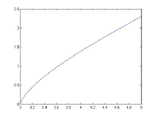
Chose an initial point r0=1subscript𝑟01r_{0}=1, we get rsuperscript𝑟r^{*}(with the stopping criterion |rnrn+1|<1010subscript𝑟𝑛subscript𝑟𝑛1superscript1010|r_{n}-r_{n+1}|<10^{-10}). Table 1 and Figure 5 show the relation of Lmaxsubscript𝐿𝑚𝑎𝑥L_{max} to E𝐸E.

Table 1. Lmaxsubscript𝐿𝑚𝑎𝑥L_{max} for different E𝐸E
E Lmaxsubscript𝐿𝑚𝑎𝑥L_{max}
3.2 0.452787235493472
3.4 0.731586885359610
3.6 0.969996239842229
3.8 1.186531828839693
4.0 1.388987957485868
4.2 1.581703995145215
4.4 1.767449993848502
4.6 1.948250754546466
4.8 2.125722162034805
5.0 2.301341325775183
Refer to caption
Figure 5. relationship of Lmaxsubscript𝐿𝑚𝑎𝑥L_{max} and E𝐸E

For L<Lmax,𝐿subscript𝐿𝑚𝑎𝑥L<L_{max}, we apply Newton’s iteration

rn+1=rnEU(r)L2/2r2U(r)+L2/r3subscript𝑟𝑛1subscript𝑟𝑛𝐸𝑈𝑟superscript𝐿22superscript𝑟2superscript𝑈𝑟superscript𝐿2superscript𝑟3r_{n+1}=r_{n}-\dfrac{E-U(r)-L^{2}/2r^{2}}{-U^{\prime}(r)+L^{2}/r^{3}}

to solve (12) with the choice of initial value

r1,0={0.1whenL>0.05,0.001whenL0.05,r2,0=2,formulae-sequencesubscript𝑟10cases0.1when𝐿0.050.001when𝐿0.05subscript𝑟202r_{1,0}=\left\{\begin{array}[c]{l}0.1\quad\text{when}\quad L>0.05,\\ 0.001\quad\text{when}\quad L\leq 0.05\end{array}\right.,\qquad r_{2,0}=2,

and the stopping criterion |rnrn+1|<1010subscript𝑟𝑛subscript𝑟𝑛1superscript1010|r_{n}-r_{n+1}|<10^{-10}. We show two graphs of EU(r)L2/2r2𝐸𝑈𝑟superscript𝐿22superscript𝑟2E-U(r)-L^{2}/2r^{2} in Figures 7, and 7

Refer to caption
Figure 6. E𝐸E=4.54.54.5,L𝐿L=0.5
Refer to caption
Figure 7. E𝐸E=4.8,L𝐿L=1.2

and the computation results are

r1=0.288701795314679,r2=1.843722113067511for Figure 7formulae-sequencesubscript𝑟10.288701795314679subscript𝑟21.843722113067511for Figure 7r_{1}=0.288701795314679,\ r_{2}=1.843722113067511\quad\text{for Figure \ref{E4_5L0_5}}
r1=0.634700793130700,r2=1.938943620330099for Figure 7formulae-sequencesubscript𝑟10.634700793130700subscript𝑟21.938943620330099for Figure 7r_{1}=0.634700793130700,\ r_{2}=1.938943620330099\quad\text{for Figure \ref{E4_8L1_2}}

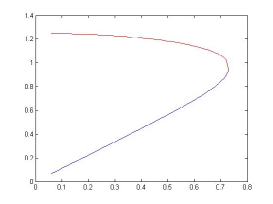
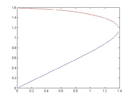
Figures 9 and 9 show how r1subscript𝑟1r_{1} and r2subscript𝑟2r_{2} (r1<r2)subscript𝑟1subscript𝑟2\left(r_{1}<r_{2}\right)\ change with respect to L𝐿L, when E𝐸E is given. (Note that the equation (12) has a unique root rsuperscript𝑟r^{\ast}\ when L=Lmax𝐿subscript𝐿L=L_{\max}, thus when L𝐿L approaches Lmaxsubscript𝐿𝑚𝑎𝑥L_{max}, the distance r2r1subscript𝑟2subscript𝑟1r_{2}-r_{1}tends to zero.)

Refer to caption
Figure 8. E𝐸E=3.4, how r1,r2subscript𝑟1subscript𝑟2r_{1},r_{2} change with L𝐿L
Refer to caption
Figure 9. E𝐸E=4, how r1,r2subscript𝑟1subscript𝑟2r_{1},r_{2} change with L𝐿L

Step 3. Computing A(ϕ,ϕ)𝐴italic-ϕitalic-ϕA(\phi,\phi) in (6). Denote the integrand

(E,L)=f0(E,L)r1(E,L)r2(E,L)(ϕϕ¯)22Ldr2(EU0(r)L2/2r2).𝐸𝐿superscriptsubscript𝑓0𝐸𝐿superscriptsubscript𝑟1𝐸𝐿𝑟2𝐸𝐿superscriptitalic-ϕ¯italic-ϕ22𝐿𝑑𝑟2𝐸subscript𝑈0𝑟superscript𝐿22superscript𝑟2\mathcal{I}(E,L)=f_{0}^{\prime}(E,L)\int_{r1(E,L)}^{r2(E,L)}(\phi-\overline{\phi})^{2}\frac{2Ldr}{\sqrt{2(E-U_{0}(r)-L^{2}/2r^{2})}}.

Choose ϕ=eritalic-ϕsuperscript𝑒𝑟\phi=e^{-r}, Table 2 shows some of the values of (E,L)𝐸𝐿\mathcal{I}(E,L).

Table 2. the value of (E,L)𝐸𝐿\mathcal{I}(E,L) for given E𝐸E and L𝐿L
(E,L)𝐸𝐿(E,L) intergrand(E,L)𝑖𝑛𝑡𝑒𝑟𝑔𝑟𝑎𝑛𝑑𝐸𝐿intergrand(E,L)
(4.1,0.6) 0.002530474111772
(4.3,1) 0.053619816035575
(4.5,1.2) -0.086444987713539
(4.7,1.3) -0.086591041429108
(4.9,1.7) -0.066267498867856

For given E𝐸E, the integration interval of (E,L)𝐸𝐿\mathcal{I}(E,L) in (6) is [0,Lmax]0subscript𝐿𝑚𝑎𝑥[0,L_{max}] for L𝐿L. When L=0𝐿0L=0 and L=Lmax𝐿subscript𝐿𝑚𝑎𝑥L=L_{max}, (7) has only one solution instead of two. To avoid this problem, we integrate (E,L)𝐸𝐿\mathcal{I}(E,L) for L𝐿L in the truncated interval [a1,Lmaxa2]subscript𝑎1subscript𝐿𝑚𝑎𝑥subscript𝑎2[a_{1},L_{max}-a_{2}], where a1,a2>0subscript𝑎1subscript𝑎20a_{1},a_{2}>0. Choose a2=105subscript𝑎2superscript105a_{2}=10^{-5}, and compare the value of a1Lmaxa2(E,L)𝑑Lsuperscriptsubscriptsubscript𝑎1subscript𝐿𝑚𝑎𝑥subscript𝑎2𝐸𝐿differential-d𝐿\int_{a_{1}}^{L_{max}-a_{2}}\mathcal{I}(E,L)dL when a1=0.01subscript𝑎10.01a_{1}=0.01 and a1=0.001subscript𝑎10.001a_{1}=0.001 in Table 3. We see that the error is approximately 107superscript10710^{-7}.

Table 3. Value of a1Lmaxa2(E,L)𝑑Lsuperscriptsubscriptsubscript𝑎1subscript𝐿𝑚𝑎𝑥subscript𝑎2𝐸𝐿differential-d𝐿\int_{a_{1}}^{L_{max}-a_{2}}\mathcal{I}(E,L)dL for a1=0.01subscript𝑎10.01a_{1}=0.01 and a1=0.001subscript𝑎10.001a_{1}=0.001
a1=0.01subscript𝑎10.01a_{1}=0.01 a1=0.001subscript𝑎10.001a_{1}=0.001
intergrandE(4.3)𝑖𝑛𝑡𝑒𝑟𝑔𝑟𝑎𝑛𝑑𝐸4.3intergrandE(4.3) 0.057831884696931 0.057831864357174
intergrandE(4.5)𝑖𝑛𝑡𝑒𝑟𝑔𝑟𝑎𝑛𝑑𝐸4.5intergrandE(4.5) -0.084810940209437 -0.084810952811088
intergrandE(4.7)𝑖𝑛𝑡𝑒𝑟𝑔𝑟𝑎𝑛𝑑𝐸4.7intergrandE(4.7) -0.095869703408813 -0.095869701098749
intergrandE(4.9)𝑖𝑛𝑡𝑒𝑟𝑔𝑟𝑎𝑛𝑑𝐸4.9intergrandE(4.9) -0.058302133990229 -0.058302146458761

Step 4. Error Estimate. Next we give a theoretical estimate for the error introduced by the truncation. Let A(E)=0r(E)dr2(EU(r)),𝐴𝐸superscriptsubscript0𝑟𝐸𝑑𝑟2𝐸𝑈𝑟A(E)=\int_{0}^{r(E)}\frac{dr}{\sqrt{2(E-U(r))}}, where r(E)𝑟𝐸r(E) is the unique solution of EU(r)=0𝐸𝑈𝑟0E-U(r)=0. For ϕ(r)=eritalic-ϕ𝑟superscript𝑒𝑟\phi(r)=e^{-r}, the error term for L𝐿L on [0,a1]0subscript𝑎1[0,a_{1}] is

(14) |32π3450a1μ(E)L4r1(E,L)r2(E,L)(ϕϕ¯)22LdrdLdE2(EU(r)L2/2r2)|32superscript𝜋3superscriptsubscript45superscriptsubscript0subscript𝑎1superscript𝜇𝐸superscript𝐿4superscriptsubscriptsubscript𝑟1𝐸𝐿subscript𝑟2𝐸𝐿superscriptitalic-ϕ¯italic-ϕ22𝐿𝑑𝑟𝑑𝐿𝑑𝐸2𝐸𝑈𝑟superscript𝐿22superscript𝑟2\displaystyle\left|32\pi^{3}\int_{4}^{5}\int_{0}^{a_{1}}\mu^{\prime}\left(E\right)L^{4}\int_{r_{1}(E,L)}^{r_{2}(E,L)}(\phi-\overline{\phi})^{2}\frac{2LdrdLdE}{\sqrt{2(E-U(r)-L^{2}/2r^{2})}}\newline \right|
646π345|μ(E)|max{A(E),T(E,a1)}𝑑Ea16.absent646superscript𝜋3superscriptsubscript45superscript𝜇𝐸𝐴𝐸𝑇𝐸subscript𝑎1differential-d𝐸superscriptsubscript𝑎16\displaystyle\leq\frac{64}{6}\pi^{3}\int_{4}^{5}|\mu^{\prime}(E)|\max\left\{A\left(E\right),T\left(E,a_{1}\right)\right\}dE\ a_{1}^{6}.

In the above, we use the estimate

T(E,L)=r1(E,L)r2(E,L)dr2(EU0L2/2r2)max{A(E),T(E,a1)}𝑇𝐸𝐿superscriptsubscriptsubscript𝑟1𝐸𝐿subscript𝑟2𝐸𝐿𝑑𝑟2𝐸subscript𝑈0superscript𝐿22superscript𝑟2𝐴𝐸𝑇𝐸subscript𝑎1T(E,L)=\int_{r_{1}(E,L)}^{r_{2}(E,L)}\frac{dr}{\sqrt{2(E-U_{0}-L^{2}/2r^{2})}}\leq\max\{A(E),T(E,a_{1})\}

due to the facts that limL0+T(E,L)=A(E)subscript𝐿limit-from0𝑇𝐸𝐿𝐴𝐸\lim_{L\rightarrow 0+}T\left(E,L\right)=A\left(E\right) and T(E,L)𝑇𝐸𝐿T\left(E,L\right) is monotone for L𝐿L\ on the small interval [0,a1]0subscript𝑎1\left[0,a_{1}\right]. We numerically compute the coefficient on the right side of (14) by choosing a1=0.01subscript𝑎10.01a_{1}=0.01, then

646π345|μ(E)|max{A(E),T(E,a1)}𝑑E=3.787856674901141×102.646superscript𝜋3superscriptsubscript45superscript𝜇𝐸𝐴𝐸𝑇𝐸subscript𝑎1differential-d𝐸3.787856674901141superscript102\frac{64}{6}\pi^{3}\int_{4}^{5}|\mu^{\prime}(E)|\max\left\{A\left(E\right),T\left(E,a_{1}\right)\right\}dE=3.787856674901141\times 10^{2}.

Thus a1=0.01subscript𝑎10.01a_{1}=0.01 is enough to make the first error to be of order 1010superscript101010^{-10}.

The error on [Lmaxa2,Lmax]subscript𝐿𝑚𝑎𝑥subscript𝑎2subscript𝐿𝑚𝑎𝑥[L_{max}-a_{2},L_{max}] is

(15) |32π345Lmaxa2Lmaxμ(E)L4r1(E,L)r2(E,L)(ϕϕ¯)22LdrdLdE2(EU(r)L2/2r2)|32superscript𝜋3superscriptsubscript45superscriptsubscriptsubscript𝐿𝑚𝑎𝑥subscript𝑎2subscript𝐿𝑚𝑎𝑥superscript𝜇𝐸superscript𝐿4superscriptsubscriptsubscript𝑟1𝐸𝐿subscript𝑟2𝐸𝐿superscriptitalic-ϕ¯italic-ϕ22𝐿𝑑𝑟𝑑𝐿𝑑𝐸2𝐸𝑈𝑟superscript𝐿22superscript𝑟2\displaystyle\ \ \ \ \left|32\pi^{3}\int_{4}^{5}\int_{L_{max}-a_{2}}^{L_{max}}\mu^{\prime}\left(E\right)L^{4}\int_{r_{1}(E,L)}^{r_{2}(E,L)}(\phi-\overline{\phi})^{2}\frac{2LdrdLdE}{\sqrt{2(E-U(r)-L^{2}/2r^{2})}}\newline \right|
64π345Lmax(E)5|μ(E)|max{πϕeff′′(r;Lmax),T(E,Lmaxa2)}𝑑Ea2.absent64superscript𝜋3superscriptsubscript45subscript𝐿𝑚𝑎𝑥superscript𝐸5superscript𝜇𝐸𝜋superscriptsubscriptitalic-ϕeff′′superscript𝑟subscript𝐿𝑇𝐸subscript𝐿subscript𝑎2differential-d𝐸subscript𝑎2\displaystyle\leq 64\pi^{3}\int_{4}^{5}L_{max}(E)^{5}|\mu^{\prime}(E)|\max\left\{\frac{\pi}{\sqrt{\phi_{\text{eff}}^{\prime\prime}\left(r^{\ast};L_{\max}\right)}},T\left(E,L_{\max}-a_{2}\right)\right\}dE\ a_{2}.

where the effective potential

ϕeff(r)=U0(r)+L2/2r2subscriptitalic-ϕeff𝑟subscript𝑈0𝑟superscript𝐿22superscript𝑟2\phi_{\text{eff}}(r)=U_{0}(r)+L^{2}/2r^{2}

Since

T(E,L)max{πϕeff′′(r;Lmax),T(E,Lmaxa2)},L[Lmaxa2,Lmax],formulae-sequence𝑇𝐸𝐿𝜋superscriptsubscriptitalic-ϕeff′′superscript𝑟subscript𝐿𝑇𝐸subscript𝐿subscript𝑎2𝐿subscript𝐿subscript𝑎2subscript𝐿T(E,L)\leq\max\left\{\frac{\pi}{\sqrt{\phi_{\text{eff}}^{\prime\prime}\left(r^{\ast};L_{\max}\right)}},T\left(E,L_{\max}-a_{2}\right)\right\},\ L\in\left[L_{\max}-a_{2},L_{\max}\right],

due to the facts that limLLmaxT(E,L)=πϕeff′′(r;Lmax)subscript𝐿subscript𝐿limit-from𝑇𝐸𝐿𝜋superscriptsubscriptitalic-ϕeff′′superscript𝑟subscript𝐿\lim_{L\rightarrow L_{\max-}}T\left(E,L\right)=\frac{\pi}{\sqrt{\phi_{\text{eff}}^{\prime\prime}\left(r^{\ast};L_{\max}\right)}} and T(E,L)𝑇𝐸𝐿T\left(E,L\right) is monotone forL𝐿\ L\ on [Lmaxa2,Lmax]subscript𝐿subscript𝑎2subscript𝐿\left[L_{\max}-a_{2},L_{\max}\right].

Numerically computing the coefficient before a2subscript𝑎2a_{2} in the right hand side of (15), we get 0.6052759134748300.6052759134748300.605275913474830. Choose a2=105subscript𝑎2superscript105a_{2}=10^{-5}, the right side of (15) if of order 105superscript10510^{-5}, which is good enough for what we need later on.

Step 5. Conclusion. We choose ϕ(r)=eritalic-ϕ𝑟superscript𝑒𝑟\phi(r)=e^{-r}. The first term of (6) is |ϕ|2=πsuperscriptitalic-ϕ2𝜋\int|\nabla\phi|^{2}=\pi, and the second term is computed to be 31.73353599866055031.733535998660550-31.733535998660550, by choosing h=0.10.1h=0.1\ in Runga-Kutta Method when solving U(r)𝑈𝑟U(r). Therefore (Aϕ,ϕ)=π31.733535998660550<0𝐴italic-ϕitalic-ϕ𝜋31.7335359986605500(A\phi,\phi)=\pi-31.733535998660550<0. We gradually decrease hh, and repeat the whole process to calculate the second term of (6). The result is shown in Table 4.

Table 4. results for different hh
hh the second term
0.1 -31.733535998660550
0.05 -38.227746546049751
0.025 -41.848643231095494
0.01 -44.146480909452201
0.005 -44.933896897054382
0.0025 -45.331673900274509
0.001 -45.571655158578380

Thus when hh becomes smaller, the second term of (6))) is less than 4545-45. Combining with the error estimates of (14) and (15) in Step 4, we can ensure (A0ϕ,ϕ)<0subscript𝐴0italic-ϕitalic-ϕ0(A_{0}\phi,\phi)<0.

3.2. Numerical Computation for Example 2

With profile (9), we choose ϕ(r)italic-ϕ𝑟\phi(r) to be a linear combination of several functions eαir, 1in,ϕ(r)=aieαirformulae-sequencesuperscript𝑒subscript𝛼𝑖𝑟1𝑖𝑛italic-ϕ𝑟subscript𝑎𝑖superscript𝑒subscript𝛼𝑖𝑟e^{-\alpha_{i}r},\ 1\leq i\leq n,\ \phi(r)=\sum a_{i}e^{-\alpha_{i}r}, with aisubscript𝑎𝑖a_{i} to be determined. In the quadratic form (6), the first term is computed to be

|ϕ|2=4π(ai24αi+4αiαj(αi+αj)3aiaj)biai2+2bijaiajsuperscriptitalic-ϕ24𝜋superscriptsubscript𝑎𝑖24subscript𝛼𝑖4subscript𝛼𝑖subscript𝛼𝑗superscriptsubscript𝛼𝑖subscript𝛼𝑗3subscript𝑎𝑖subscript𝑎𝑗subscript𝑏𝑖superscriptsubscript𝑎𝑖22subscript𝑏𝑖𝑗subscript𝑎𝑖subscript𝑎𝑗\displaystyle\int|\nabla\phi|^{2}=4\pi(\sum\frac{a_{i}^{2}}{4\alpha_{i}}+\sum\frac{4\alpha_{i}\alpha_{j}}{(\alpha_{i}+\alpha_{j})^{3}}a_{i}a_{j})\newline \triangleq\sum b_{i}a_{i}^{2}+2\sum b_{ij}a_{i}a_{j}

and the second term is

32π3f0(E,L)r1(E,L)r2(E,L)(aiϕiaiϕi¯)22LdrdEdL2(EU0(r)L2/2r2)32superscript𝜋3superscriptsubscript𝑓0𝐸𝐿superscriptsubscript𝑟1𝐸𝐿𝑟2𝐸𝐿superscriptsubscript𝑎𝑖subscriptitalic-ϕ𝑖¯subscript𝑎𝑖subscriptitalic-ϕ𝑖22𝐿𝑑𝑟𝑑𝐸𝑑𝐿2𝐸subscript𝑈0𝑟superscript𝐿22superscript𝑟2\displaystyle 32\pi^{3}\int f_{0}^{\prime}(E,L)\int_{r1(E,L)}^{r2(E,L)}(\sum a_{i}\phi_{i}-\overline{\sum a_{i}\phi_{i}})^{2}\frac{2LdrdEdL}{\sqrt{2(E-U_{0}(r)-L^{2}/2r^{2})}}
=32π3f0(E,L)r1(E,L)r2(E,L)(ϕiϕi¯)22LdrdEdL2(EU0(r)L2/2r2)ai2+absentlimit-from32superscript𝜋3superscriptsubscript𝑓0𝐸𝐿superscriptsubscript𝑟1𝐸𝐿𝑟2𝐸𝐿superscriptsubscriptitalic-ϕ𝑖¯subscriptitalic-ϕ𝑖22𝐿𝑑𝑟𝑑𝐸𝑑𝐿2𝐸subscript𝑈0𝑟superscript𝐿22superscript𝑟2superscriptsubscript𝑎𝑖2\displaystyle=\sum 32\pi^{3}\int f_{0}^{\prime}(E,L)\int_{r1(E,L)}^{r2(E,L)}(\phi_{i}-\overline{\phi_{i}})^{2}\frac{2LdrdEdL}{\sqrt{2(E-U_{0}(r)-L^{2}/2r^{2})}}a_{i}^{2}+
32π3f0(E,L)r1(E,L)r2(E,L)(ϕiϕi¯)(ϕjϕj¯)2LdrdEdL2(EU0(r)L2/2r2)2aiaj32superscript𝜋3superscriptsubscript𝑓0𝐸𝐿superscriptsubscript𝑟1𝐸𝐿𝑟2𝐸𝐿subscriptitalic-ϕ𝑖¯subscriptitalic-ϕ𝑖subscriptitalic-ϕ𝑗¯subscriptitalic-ϕ𝑗2𝐿𝑑𝑟𝑑𝐸𝑑𝐿2𝐸subscript𝑈0𝑟superscript𝐿22superscript𝑟22subscript𝑎𝑖subscript𝑎𝑗\displaystyle\sum 32\pi^{3}\int f_{0}^{\prime}(E,L)\int_{r1(E,L)}^{r2(E,L)}(\phi_{i}-\overline{\phi_{i}})(\phi_{j}-\overline{\phi_{j}})\frac{2LdrdEdL}{\sqrt{2(E-U_{0}(r)-L^{2}/2r^{2})}}2a_{i}a_{j}
ciai2+2cijaiajabsentsubscript𝑐𝑖superscriptsubscript𝑎𝑖22subscript𝑐𝑖𝑗subscript𝑎𝑖subscript𝑎𝑗\displaystyle\triangleq\sum c_{i}a_{i}^{2}+\sum 2c_{ij}a_{i}a_{j}

Now (A0ϕ,ϕ)=(bi+ci)ai2+2(bij+cij)aiaj.subscript𝐴0italic-ϕitalic-ϕsubscript𝑏𝑖subscript𝑐𝑖superscriptsubscript𝑎𝑖22subscript𝑏𝑖𝑗subscript𝑐𝑖𝑗subscript𝑎𝑖subscript𝑎𝑗(A_{0}\phi,\phi)=\sum(b_{i}+c_{i})a_{i}^{2}+2\sum(b_{ij}+c_{ij})a_{i}a_{j}. The corresponding matrix for this quadratic form is S=(sij)𝑆subscript𝑠𝑖𝑗S=(s_{ij}), where sii=bi+ci,sij=bij+cijformulae-sequencesubscript𝑠𝑖𝑖subscript𝑏𝑖subscript𝑐𝑖subscript𝑠𝑖𝑗subscript𝑏𝑖𝑗subscript𝑐𝑖𝑗s_{ii}=b_{i}+c_{i},\quad s_{ij}=b_{ij}+c_{ij}. Denote λminsubscript𝜆\lambda_{\min} to be the minimum eigenvalue of the matrix S𝑆S, then λmin<0subscript𝜆0\lambda_{\min}<0 guarantees that there exists ϕitalic-ϕ\phi such that (A0ϕ,ϕ)<0subscript𝐴0italic-ϕitalic-ϕ0(A_{0}\phi,\phi)<0. We choose

ϕ1=er,ϕ2=e12r,ϕ3=e13r,ϕ4=e2r,ϕ5=e3r,ϕ6=e4r,ϕ7=e5r.formulae-sequencesubscriptitalic-ϕ1superscript𝑒𝑟formulae-sequencesubscriptitalic-ϕ2superscript𝑒12𝑟formulae-sequencesubscriptitalic-ϕ3superscript𝑒13𝑟formulae-sequencesubscriptitalic-ϕ4superscript𝑒2𝑟formulae-sequencesubscriptitalic-ϕ5superscript𝑒3𝑟formulae-sequencesubscriptitalic-ϕ6superscript𝑒4𝑟subscriptitalic-ϕ7superscript𝑒5𝑟\phi_{1}=e^{-r},\ \phi_{2}=e^{-\frac{1}{2}r},\ \phi_{3}=e^{-\frac{1}{3}r},\ \phi_{4}=e^{-2r},\ \phi_{5}=e^{-3r},\ \phi_{6}=e^{-4r},\ \phi_{7}=e^{-5r}.\quad

In (9), there are five free parameters in μ𝜇\mu: a,k,t1,E0,C1𝑎𝑘subscript𝑡1subscript𝐸0subscript𝐶1a,k,t_{1},E_{0},C_{1} and E1subscript𝐸1E_{1} is determined by E1=(E0+t1a)/(t1+1)subscript𝐸1subscript𝐸0subscript𝑡1𝑎subscript𝑡11E_{1}=(E_{0}+t_{1}a)/(t_{1}+1). Using U0subscript𝑈0U_{0} (the initial value of the potential) as an additional parameter, there are totally six parameters in our calculations. The idea is to view λminsubscript𝜆𝑚𝑖𝑛\lambda_{min} as a function of these parameters λmin=λmin(a,k,t1,E0,C1,U0).subscript𝜆𝑚𝑖𝑛subscript𝜆𝑚𝑖𝑛𝑎𝑘subscript𝑡1subscript𝐸0subscript𝐶1subscript𝑈0\lambda_{min}=\lambda_{min}(a,k,t_{1},E_{0},C_{1},U_{0}). Our goal now is to find proper parameters such that λmin<0.subscript𝜆𝑚𝑖𝑛0\lambda_{min}<0. The numerical methods are the same as in Step 1-Step 3 in the computation of Example 1, except that now we use self-adaptive Runge-Kutta Method to solve (11). We next verify that the following choice of parameters

C1=2,E0=5.1,a=1.9,k=2.01,t1=1.5,U0=15.1,formulae-sequencesubscript𝐶12formulae-sequencesubscript𝐸05.1formulae-sequence𝑎1.9formulae-sequence𝑘2.01formulae-sequencesubscript𝑡11.5subscript𝑈015.1C_{1}=2,\ E_{0}=5.1,\ a=1.9,\ k=2.01,\ t_{1}=1.5,\ U_{0}=-15.1,

would lead to λmin<0subscript𝜆𝑚𝑖𝑛0\lambda_{min}<0\ and(A0ϕ,ϕ)<0subscript𝐴0italic-ϕitalic-ϕ0\ (A_{0}\phi,\phi)<0. In Table 5 we show the results of λminsubscript𝜆\lambda_{\min} under different accuracies.

Table 5. λminsubscript𝜆𝑚𝑖𝑛\lambda_{min} under different accuracies
integration accuracy a1subscript𝑎1a_{1} a2subscript𝑎2a_{2} accuracy of the roots λminsubscript𝜆𝑚𝑖𝑛\lambda_{min}
108superscript10810^{-8} 105superscript10510^{-5} 106superscript10610^{-6} 1010superscript101010^{-10} 1.808068979998836×1051.808068979998836superscript105-1.808068979998836\times 10^{-5}
109superscript10910^{-9} 103superscript10310^{-3} 104superscript10410^{-4} 1010superscript101010^{-10} 3.403231868973289×1063.403231868973289superscript106-3.403231868973289\times 10^{-6}
109superscript10910^{-9} 105superscript10510^{-5} 106superscript10610^{-6} 1011superscript101110^{-11} 3.739973399333609×1063.739973399333609superscript106-3.739973399333609\times 10^{-6}
1010superscript101010^{-10} 105superscript10510^{-5} 106superscript10610^{-6} 1011superscript101110^{-11} 3.196606813186484×1063.196606813186484superscript106-3.196606813186484\times 10^{-6}
1011superscript101110^{-11} 105superscript10510^{-5} 106superscript10610^{-6} 1011superscript101110^{-11} 3.025099283901562×1063.025099283901562superscript106-3.025099283901562\times 10^{-6}
1012superscript101210^{-12} 106superscript10610^{-6} 107superscript10710^{-7} 1011superscript101110^{-11} 3.087487453314562×1063.087487453314562superscript106-3.087487453314562\times 10^{-6}
1013superscript101310^{-13} 106superscript10610^{-6} 107superscript10710^{-7} 1011superscript101110^{-11} 3.080483943121587×1063.080483943121587superscript106-3.080483943121587\times 10^{-6}
1013superscript101310^{-13} 106superscript10610^{-6} 107superscript10710^{-7} 1011superscript101110^{-11} 3.089704058599446×1063.089704058599446superscript106-3.089704058599446\times 10^{-6}
1014superscript101410^{-14} 107superscript10710^{-7} 107superscript10710^{-7} 1011superscript101110^{-11} 3.089187445892979×1063.089187445892979superscript106-3.089187445892979\times 10^{-6}

where a1subscript𝑎1a_{1} and a2subscript𝑎2a_{2} are the parameters used to truncate [0,Lmax]0subscript𝐿[0,L_{\max}] to [a1,Lmaxa2]subscript𝑎1subscript𝐿subscript𝑎2[a_{1},L_{\max}-a_{2}]. We also calculate the eigenvector corresponding to λminsubscript𝜆\lambda_{\min}\ by v=(v1,v2,v3,v4,v5,v6,v7)Tvsuperscriptsubscript𝑣1subscript𝑣2subscript𝑣3subscript𝑣4subscript𝑣5subscript𝑣6subscript𝑣7𝑇\mathbf{\emph{v}}=(v_{1},v_{2},v_{3},v_{4},v_{5},v_{6},v_{7})^{T}, where

(16) v1=41.702767064740subscript𝑣141.702767064740\displaystyle v_{1}=41.702767064740
v2=14.949618378683subscript𝑣214.949618378683\displaystyle v_{2}=-14.949618378683
v3=4.856846351504subscript𝑣34.856846351504\displaystyle v_{3}=4.856846351504
v4=201.361293458803subscript𝑣4201.361293458803\displaystyle v_{4}=-201.361293458803
v5=571.694416252419subscript𝑣5571.694416252419\displaystyle v_{5}=571.694416252419
v6=723.292461038838subscript𝑣6723.292461038838\displaystyle v_{6}=-723.292461038838
v7=327.842857021134.subscript𝑣7327.842857021134\displaystyle v_{7}=327.842857021134.

Let

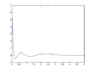
ϕ(r)=v1er+v2e12r+v3e13r+v4e2r+v5e3r+v6e4r+v7e5r.italic-ϕ𝑟subscript𝑣1superscript𝑒𝑟subscript𝑣2superscript𝑒12𝑟subscript𝑣3superscript𝑒13𝑟subscript𝑣4superscript𝑒2𝑟subscript𝑣5superscript𝑒3𝑟subscript𝑣6superscript𝑒4𝑟subscript𝑣7superscript𝑒5𝑟\phi(r)=v_{1}e^{-r}+v_{2}e^{-\frac{1}{2}r}+v_{3}e^{-\frac{1}{3}r}+v_{4}e^{-2r}+v_{5}e^{-3r}+v_{6}e^{-4r}+v_{7}e^{-5r}.

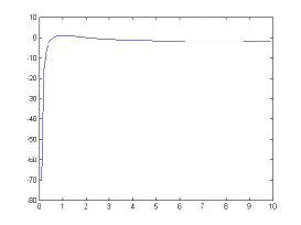
We draw a picture of this function ϕitalic-ϕ\phi in Figure 10.

Refer to caption
Figure 10. ϕ(r)italic-ϕ𝑟\phi(r)

Using (6), we obtain

(Aϕ,ϕ)=35.23148486628272059.247837621248109<0,𝐴italic-ϕitalic-ϕ35.23148486628272059.2478376212481090(A\phi,\phi)=35.231484866282720-59.247837621248109<0,

when the integration accuracy is 1013superscript101310^{-13},a1=106subscript𝑎1superscript106\ a_{1}=10^{-6},a2=107subscript𝑎2superscript107\ a_{2}=10^{-7}, and the root accuracy is 1011superscript101110^{-11}.

Step 4. Error Estimate. We obtain theoretical error estimate as in Example 1. For any test function ϕitalic-ϕ\phi, the error for L𝐿L on [0,a1]0subscript𝑎1[0,a_{1}] is

|32π3{E|μ(E)>0}μ(E)0a1r1(E,L)r2(E,L)(ϕϕ¯)22LdrdLdE2(EU0L2/2r2)|32superscript𝜋3subscriptconditional-set𝐸superscript𝜇𝐸0superscript𝜇𝐸superscriptsubscript0subscript𝑎1superscriptsubscriptsubscript𝑟1𝐸𝐿subscript𝑟2𝐸𝐿superscriptitalic-ϕ¯italic-ϕ22𝐿𝑑𝑟𝑑𝐿𝑑𝐸2𝐸subscript𝑈0superscript𝐿22superscript𝑟2\displaystyle\left|32\pi^{3}\int_{\{E|\mu^{\prime}(E)>0\}}\mu^{\prime}(E)\int_{0}^{a_{1}}\int_{r_{1}(E,L)}^{r_{2}(E,L)}(\phi-\overline{\phi})^{2}\frac{2LdrdLdE}{\sqrt{2(E-U_{0}-L^{2}/2r^{2})}}\right|
\displaystyle\leq 32π3|maxϕminϕ|2a12{E|μ(E)>0}μ(E)max{A(E),T(E,a1)}𝑑E32superscript𝜋3superscriptitalic-ϕitalic-ϕ2superscriptsubscript𝑎12subscriptconditional-set𝐸superscript𝜇𝐸0superscript𝜇𝐸𝐴𝐸𝑇𝐸subscript𝑎1differential-d𝐸\displaystyle 32\pi^{3}|\max\phi-\min\phi|^{2}a_{1}^{2}\int_{\{E|\mu^{\prime}(E)>0\}}\mu^{\prime}(E)\max\{A(E),T(E,a_{1})\}dE

Numerically compute the right hand side, and note

|maxϕminϕ|2max|ϕ|2|vi|=3.7714×10³.italic-ϕitalic-ϕ2italic-ϕ2subscript𝑣𝑖3.7714superscript103|\max\phi-\min\phi|\leq 2\max|\phi|\leq 2\sum|v_{i}|=3.7714\times 10^{3}.

Choose a1=105subscript𝑎1superscript105a_{1}=10^{-5}, the error is no more than

4.322×102×(3.7714×103)2×(105)2=6.1474×1014.322superscript102superscript3.7714superscript1032superscriptsuperscript10526.1474superscript1014.322\times 10^{2}\times(3.7714\times 10^{3})^{2}\times(10^{-5})^{2}=6.1474\times 10^{-1}

Next we estimate the error for L𝐿L on [Lmaxa2,Lmax]subscript𝐿subscript𝑎2subscript𝐿[L_{\max}-a_{2},L_{\max}]. When r[r1,r2]𝑟subscript𝑟1subscript𝑟2r\in[r_{1},r_{2}], we use |ϕϕ¯|max|ϕ|(r2r1)italic-ϕ¯italic-ϕsuperscriptitalic-ϕsubscript𝑟2subscript𝑟1|\phi-\overline{\phi}|\leq\max|\phi^{\prime}|(r_{2}-r_{1}) by the Mean Value Theorem. So the error is

32π3{E|μ(E)>0}Lmaxa2Lmaxr1(E,L)r2(E,L)μ(E)(ϕϕ¯)22LdrdLdE2(EU0L2/2r2)32superscript𝜋3subscriptconditional-set𝐸superscript𝜇𝐸0superscriptsubscriptsubscript𝐿𝑚𝑎𝑥subscript𝑎2subscript𝐿𝑚𝑎𝑥superscriptsubscriptsubscript𝑟1𝐸𝐿subscript𝑟2𝐸𝐿superscript𝜇𝐸superscriptitalic-ϕ¯italic-ϕ22𝐿𝑑𝑟𝑑𝐿𝑑𝐸2𝐸subscript𝑈0superscript𝐿22superscript𝑟2\displaystyle 32\pi^{3}\int_{\{E|\mu^{\prime}(E)>0\}}\int_{L_{max}-a_{2}}^{L_{max}}\int_{r_{1}(E,L)}^{r_{2}(E,L)}\mu^{\prime}(E)(\phi-\overline{\phi})^{2}\frac{2LdrdLdE}{\sqrt{2(E-U_{0}-L^{2}/2r^{2})}}
64π3a2|ϕ|L2{E|μ(E)>0}μ(E)Lmax(E)(r2(E,Lmaxa2)r1(E,Lmaxa2))2\displaystyle\leq 64\pi^{3}a_{2}\left|\phi^{\prime}\right|_{L^{\infty}}^{2}\int_{\left\{E|\ \mu^{\prime}\left(E\right)>0\right\}}\mu^{\prime}\left(E\right)L_{\max}\left(E\right)\left(r_{2}(E,L_{\max}-a_{2})-r_{1}(E,L_{\max}-a_{2})\right)^{2}\cdot
max{πϕeff′′(r;Lmax),T(E,Lmaxa2)}dE.𝜋superscriptsubscriptitalic-ϕeff′′superscript𝑟subscript𝐿𝑇𝐸subscript𝐿subscript𝑎2𝑑𝐸\displaystyle\max\left\{\frac{\pi}{\sqrt{\phi_{\text{eff}}^{\prime\prime}\left(r^{\ast};L_{\max}\right)}},T\left(E,L_{\max}-a_{2}\right)\right\}dE\ .

Note that

max|ϕ|5|vi|=9.4285×10³.superscriptitalic-ϕ5subscript𝑣𝑖9.4285superscript103\max\ |\phi^{\prime}|\leq 5\sum|v_{i}|=9.4285\times 10^{3}.

Numerically computation of this error with a2=107subscript𝑎2superscript107a_{2}=10^{-7} yields a bound of

1.41722×1013×(9.4285×103)2=1.3362×1061.41722superscript1013superscript9.4285superscript10321.3362superscript1061.41722\times 10^{-13}\times(9.4285\times 10^{3})^{2}=1.3362\times 10^{-6}

So the total error is at most of order 101superscript10110^{-1}, which guarantees (Aϕ,ϕ)<0.𝐴italic-ϕitalic-ϕ0(A\phi,\phi)<0.

4. Summary

We study the instability of spherical galaxy models in the Vlasov theory for collisionless stars. Based on the instability criterion of Theorem 1 and careful numerical computations, we have constructed two explicit unstable galaxy models f0(E,L)subscript𝑓0𝐸𝐿f_{0}(E,L) and f0(E)subscript𝑓0𝐸f_{0}(E) with distributions (8) and (9) respectively. In particular,f0(E)subscript𝑓0𝐸\ f_{0}(E) in Example 2 provides the first example of unstable isotropic galaxy which has not been found in literature. The instability in these examples are radial and non-oscillatory. Compared with the usual N-body codes of finding instability of galaxy models, our method only requires numerical evaluation of certain explicit integrals. Therefore, it is much more reliable and easier to implement. It is hoped that Theorem 1 can be employed to detest instability for other galaxy models in the future.

Acknowledgements 

This research is supported partly by NSF grants DMS-0603815 and DMS-0505460 (Guo) and DMS-0908175 (Lin).

References

  • [1] Antonov, V. A. Remarks on the problem of stability in stellar dynamics. Soviet Astr, AJ., 4, 859-867 (1961).
  • [2] Antonov, V. A., Solution of the problem of stability of stellar system Emden’s density law and the spherical distribution of velocities, Vestnik Leningradskogo Universiteta, Leningrad University, 1962.
  • [3] Barnes, J.; Hut, P.; Goodman, J., Dynamical instabilities in spherical stellar systems, Astrophysical Journal, vol. 300, p. 112-131, 1986.
  • [4] Bartholomew, P., On the theory of stability of galaxies, Monthly Notices of the Royal Astronomical Society, Vol. 151, p. 333 (1971).
  • [5] Bertin, Giuseppe, Dynamics of Galaxies, Cambridge University Press, 2000.
  • [6] Binney, J., Tremaine, S., Galactic Dynamics (2nd edition). Princeton University Press, 2008.
  • [7] Doremus, J. P.; Feix, M. R.; Baumann, G.; , Stability of Encounterless Spherical Stellar Systems, Phys. Rev. Letts, Vol. 26, p. 725 (1971).
  • [8] Gillon, D.; Cantus, M.; Doremus, J. P.; Baumann, G., Stability of self-gravitating spherical systems in which phase space density is a function of energy and angular momentum, for spherical perturbations, Astronomy and Astrophysics, vol. 50, no. 3, p. 467-470, 1976.
  • [9] Fridman, A., Polyachenko, V., Physics of Gravitating System Vol I and II, Springer-Verlag, 1984.
  • [10] Goodman, Jeremy, An instability test for nonrotating galaxies, Astrophysical Journal, vol. 329, p. 612-617, 1988.
  • [11] Guo, Y., Z. Lin, Unstable and stable galaxy models. Commun. Math. Phys. 279, no. 3, 789–813, 2008.
  • [12] Henon, M., Numerical Experiments on the Stability of Spherical Stellar Systems, Astronomy and Astrophysics, Vol. 24, p. 229 (1973).
  • [13] Guo, Y., Rein, G., A non-variational approach to nonlinear stability in stellar dynamics applied to the King model, Comm. Math. Phys. 271 (2007), no. 2, 489-509.
  • [14] Kandrup, H.; Signet, J. F.; A simple proof of dynamical stability for a class of spherical clusters. The Astrophys. J. 298, p. 27-33.(1985)
  • [15] Kandrup, Henry E., A stability criterion for any collisionless stellar equilibrium and some concrete applications thereof, Astrophysical Journal, vol. 370, p. 312-317, 1991.
  • [16] King, Ivan R., The structure of star clusters. III. Some simple dynamical models, Astronomical Journal, Vol. 71, p. 64 (1966).
  • [17] Merritt, David, Elliptical Galaxy Dynamics, The Publications of the Astronomical Society of the Pacific, Volume 111, Issue 756, pp. 129-168.
  • [18] Palmer, P. L., Stability of collisionless stellar systems: mechanisms for the dynamical structure of galaxies, Kluwer Academic Publishers, 1994.
  • [19] Perez, Jerome and Aly, Jean-Jacques, Stability of spherical stellar systems - I. Analytical results, Monthly Notices of the Royal Astronomical Society, Volume 280, Issue 3, pp. 689-699, 1996.
  • [20] Sygnet, J. F.; des Forets, G.; Lachieze-Rey, M.; Pellat, R., Stability of gravitational systems and gravothermal catastrophe in astrophysics, Astrophysical Journal, vol. 276, p. 737-745, 1984.
  • [21] Rein,Gerhard; Rendall,Alan D. Compact support of spherically symmetric equilibria in non-relativistic and relativistic galactic dynamics, Math. Proc. Camb. Phil. Soc. 128 (2000), 363-380.