Dynamic Credit Investment in Partially Observed Markets

Abstract

We consider the problem of maximizing expected utility for a power investor who can allocate his wealth in a stock, a defaultable security, and a money market account. The dynamics of these security prices are governed by geometric Brownian motions modulated by a hidden continuous time finite state Markov chain. We reduce the partially observed stochastic control problem to a complete observation risk sensitive control problem via the filtered regime switching probabilities. We separate the latter into pre-default and post-default dynamic optimization subproblems, and obtain two coupled Hamilton-Jacobi-Bellman (HJB) partial differential equations. We prove existence and uniqueness of a globally bounded classical solution to each HJB equation, and give the corresponding verification theorem. We provide a numerical analysis showing that the investor increases his holdings in stock as the filter probability of being in high growth regimes increases, and decreases his credit risk exposure when the filter probability of being in high default risk regimes gets larger.

Keywords and phrases: Partial information, Filtering, Risk sensitive control, Default risk, Hidden markov chain.

JEL codes:  G11, C61, C11.

MSC codes: Primary 93E20; Secondary 91B28, 49L20, 49L25.

1 Introduction

Regime switching models constitute an appealing framework, stemming from their ability to capture the relevant features of asset price dynamics, which behave differently depending on the specific phase of the business cycle in place. In the context of continuous time utility maximization, some studies have considered observable regimes, while others have accounted for the possibility that they are not directly visible. In the case of observable regimes, Zariphopoulou (1992) considers an infinite horizon investment-consumption model where the agent can invest her wealth in a stock and risk-free bond, with borrowing and stock short-selling constraints. In a similar regime switching framework, Sotomayor and Cadenillas (2009) study the infinite horizon problem of a risk averse investor maximizing regime dependent utility from terminal wealth and consumption. A different branch of literature has considered the case when regimes are hidden and need to be estimated from publicly available market information. Nagai and Runggaldier (2008) consider a finite horizon portfolio optimization problem, where a power investor allocates his wealth across money market account and stocks, whose price dynamics follow a diffusion process modulated by a hidden finite-state Markov process. Tamura and Watanabe (2011) extend the analysis to the case when the time horizon is infinite. Elliott and Siu (2011) study the optimal investment problem of an insurer when the model uncertainty is governed by a hidden Markov chain. Siu (2013) considers optimal investment problems in general non-Markovian hidden regime switching models. Sass and Haussmann (2004) consider a multi-stock market model, with stochastic interest rates and drift modulated by a hidden Markov chain. Combining appropriate Malliavin calculus and filtering results from hidden Markov models, they derive explicit representations of the optimal strategies. In a series of two papers, Fujimoto et al. (2013a) and Fujimoto et al. (2013b) consider a regime switching framework where logarithmic and power investors optimize their terminal utility by investing in stocks at random times due to liquidity constraints.

The literature surveyed above has considered markets consisting of securities carrying market, but not default, risk. In recent years, few studies have considered a portfolio optimization framework inclusive of defaultable securities. Kraft and Steffensen (2005) study optimal portfolio problems with defaultable assets within a Black-Cox framework. Kraft and Steffensen (2008) consider an investor who can allocate her wealth across multiple defaultable bonds, in a model where simultaneous defaults are allowed. In the same market model, Kraft and Steffensen (2009) define default as the beginning of financial distress, and discuss contagion effects on prices of defaultable bonds. Bielecki and Jang (2006) derive optimal investment strategies for a CRRA investor, allocating her wealth among a defaultable bond, risk-free bank account, and a stock. Bo et al. (2010) consider a portfolio optimization problem, where a logarithmic investor can choose a consumption rate, and invest her wealth across a defaultable perpetual bond, a stock, and a money market account. Jiao and Pham (2013) combine duality theory and dynamic programming to optimize the utility of a CRRA investor in a market consisting of a riskless bond and a stock subject to counterparty risk. Optimal investment under contagion risk has been considered by Bo and Capponi (2014), who construct an empirically motivated framework based on interacting intensity models, and analyze how contagion effects impact optimal allocation decisions due to abrupt changes in prices. A related study by Jiao et al. (2013) develop a portfolio framework where multiple default events can occur, and some of the securities may still be traded after default.

The first attempt at using regime switching within a portfolio optimization framework consisting of defaultable securities was done by Capponi and Figueroa-López (2014). Such a modeling choice is also empirically supported by a study of Giesecke et al. (2011), which identifies three credit regimes characterized by different levels of default intensity and recovery rates, via a historical analysis of the corporate bond market. Capponi and Figueroa-López (2014) consider an investor trading in a stock and defaultable security, whose price dynamics are modulated by an observable Markov chain. Using the HJB approach, they recover the optimal investment strategies as the unique solution to a coupled system of partial differential equations.

The present paper considers the case where regimes are hidden, so that the power investor must decide on the optimal allocation policy using only the observed market prices. This improves upon the realism of the model in Capponi and Figueroa-López (2014), given that in several circumstances market regimes such as inflation and recession, or credit regimes characterized by high or low credit spreads, are typically unobserved to investors. Moreover, the hidden regime feature requires a completely different analysis, and leads us to solving a partially observed stochastic control problem, where regime information must be inferred from an enlarged market filtration. The latter is composed both of a reference filtration generated by the observable security prices, and of a credit filtration tracking the occurrence of the default event. To the best of our knowledge, ours represents the first study in this direction.

We next describe our main contributions. First, by considering a portfolio optimization problem in a context of partial information with possibility of default, we advance earlier literature which has so far considered either one or the other aspect, but never both simultaneously. We construct an equivalent fully observed risk-sensitive control problem, where the new state is given by the regime filtered probabilities, generalizing the approach of Nagai and Runggaldier (2008) who do not deal with default event information. We use the filter probabilities to obtain the Hamilton-Jacobi-Bellman (HJB) equation for the dynamic optimization problem, which we separate it into coupled pre-default and post-default optimization subproblems. This is done using the projected filter process. We remark that the decomposition of a global optimal investment problem into sub-control problems in a progressively enlarged filtration has also been considered by Jiao et al. (2013) and Pham (2010). Their approach consists in first defining the sub-control problems in the reference market filtration exclusive of default event information, and then connecting them by assuming the existence of a conditional density on the default times, previously introduced in El Karoui et al. (2010). Despite few similarities between ours and their approach arising from the fact that both consider a pre and post-default decomposition and solve backwards, there are also significant differences between the two approaches. We consider the wealth dynamics under the enlarged market filtration inclusive of default events and do not perform any pre-post default decomposition of the control problem at the level of the stochastic differential equation. It is only after deriving the HJB partial differential equations that the decomposition into pre and post-default PDEs naturally arises. Their approach instead exploits the exponential utility preference function of the investor to reduce the optimal investment problem to solving a recursive system of backward stochastic differential equations with respect to the default-free market filtration. A detailed analysis of these BSDEs including the possibility of jump times driven by Brownian motion is provided in Kharroubi and Lim (2013).

Secondly, the presence of default risk makes the HJB-PDE satisfied by the pre-default value function non-linear. There are two sources of nonlinearity, namely quadratic growth of the gradient and exponential nonlinearity. We first perform a suitable transformation yielding a parabolic PDE whose associated operator is linear in the gradient and matrix of second derivatives, but nonlinear in the solution. We then provide a rigorous analysis of the transformed PDE and prove the existence of a classical solution via a monotone iterative method. Since the nonlinear term is only locally, but not globally, Lipschitz continuous because the derivative explodes at zero, we also need to prove that the solution is bounded away from zero. In particular, we establish both a lower and upper bound for the solution, and prove $\mathcal{C}^{2,\alpha}_{P}$ regularity. We then use this result to prove a verification theorem establishing the correspondence between the solution to the PDE and the value function of the control problem. The proof of the theorem requires the development of a number of technical results, such as the guaranteed positivity of the filtering process. By contrast, the HJB-PDE corresponding to the post-default optimization problem can be linearized using a similar transformation to the one adopted by Nagai and Runggaldier (2008), and a unique classical solution can be guaranteed as shown, for instance, in Tamura and Watanabe (2011).

Thirdly, we provide a thorough comparative statics analysis to illustrate the impact of partial information on the optimal allocation decisions. We consider a square root investor and a two-states Markov chain. We find that the fraction of wealth invested in the stock increases as the filter probability of being in the regime with the highest growth rate increases. In order to be hedged against default, the investor shorts a higher number of units of defaultable security if the filter probability of staying in the highest default risk regime increases. Vice versa, when the probability of being in the safest regime increases, the investor increases his exposure to credit risk by shorting smaller amount of units of the defaultable security. If the regime is characterized by a sufficiently low level of default intensity, the square root investor may even go long credit, and purchase units of the defaultable security. We find that lower values of price volatility induce the investor to increase the fraction of wealth invested in the risky asset. More specifically, if the stock volatility is low, the filter gain coming from received observations is higher and the investor purchases increasingly more units as the stock volatility decreases. Similarly, for a sufficiently high probability of being in the high default risk regime, the investor shorts increasingly larger number of units of defaultable security as the volatility of the latter decreases. This reflects the risk averse nature of the investor, who wants to reduce his credit risk exposure more if the filter estimate becomes more accurate due to the higher informational gain from price observations. We also find that as observations become less informative due to higher price volatilities, the investor deposits a significant fraction of his wealth in the money market account. All this suggests that partial information tends to push the investor towards strategies reducing both market and credit risk exposure.

The rest of the paper is organized as follows. Section 2 defines the market model. Section 3 sets up the utility maximization problem. Section 4 derives the HJB equations corresponding to the risk sensitive control problem. Section 5 analyzes the solutions of the HJB-PDE equations. Section 6 develops a numerical analysis. Section 7 summarizes our main conclusions. Finally, two appendices present the main proofs of the paper.

2 The Market Model

Assume $(\Omega,\mathcal{G},\mathbb{G},\mathbb{P})$ is a complete filtered probability space, where $\mathbb{P}$ is the historical probability measure, ${\mathbb{G}}:=(\mathcal{G}_{t})_{t\geq 0}$ is an enlarged filtration given by $\mathcal{G}_{t}:=\mathcal{F}_{t}\vee\mathcal{H}_{t}$, where $(\mathcal{H}_{t})_{t}$ is a filtration to be introduced below. We take the right continuous version of $\mathbb{G}$, i.e. $\mathcal{G}_{t}$ is the smallest right-continuous filtration containing $\mathbb{F}$ and $\mathbb{H}$, with $\mathcal{G}_{t}:=\bigcap_{\epsilon>0}\left(\mathcal{F}_{t+\epsilon}\vee\mathcal{H}_{t+\epsilon}\right)$ (see also Belanger et al. (2004)).

Here, $\mathbb{F}:=(\mathcal{F}_{t})_{t}$ is a suitable filtration supporting a two dimensional Brownian motion $W_{t}=(W_{t}^{(1)},W_{t}^{(2)})^{\top}$, where ^⊤ denotes the transpose. We also assume that the hidden states of the economy are modeled by a finite-state continuous-time Markov chain $X:=\{X_{t}\}_{t\geq{}0}$, which is adapted to $\mathbb{G}$ and assumed to be independent of $W:=\{W_{t}\}_{t\geq{}0}$. Without loss of generality, the state space is identified by the set of unit vectors $\{e_{1},e_{2},\ldots,e_{N}\}$, where $e_{i}=(0,...,1,...0)^{{}^{\top}}\in\mathds{R}^{N}$. The following semi-martingale representation is well-known (cf. Elliott et al. (1994)):

$$X_{t}=X_{0}+\int_{0}^{t}{A(s)^{\top}}X_{s}ds+{\varphi(t)}{,}$$ (1)

where $\varphi(t)=(\varphi_{1}(t),\dots,\varphi_{N}(t))^{\top}$ is a $\mathds{R}^{N}$-valued martingale under $\mathbb{P}$, and $A(t):=[\varpi_{i,j}(t)]_{i,j=1,\dots,N}$ is the so-called generator of the Markov process. Specifically, denoting $p_{i,j}(t,s):=\mathbb{P}(X_{s}=e_{j}|X_{t}=e_{i})$, for $s\geq t$, and $\delta_{i,j}={\bf 1}_{i=j}$, we have that

$$\varpi_{i,j}(t)=\lim_{h\rightarrow 0}\frac{p_{i,j}(t,t+h)-\delta_{i,j}}{h};$$

cf. Bielecki and Rutkowski (2001). In particular, $\varpi_{i,i}(t)=-\sum_{j\neq i}\varpi_{i,j}(t)$. The following mild condition is also imposed:

$$\sup_{t\geq{}0}\max_{i,j}\varpi_{i,j}(t)<\infty.$$ (2)

We denote by $p^{\circ}=(p^{\circ,1},\ldots,p^{\circ,N})$ the initial distribution on the Markov chain and, throughout the paper, assume that $p^{\circ,i}>0$.

We consider a frictionless financial market consisting of three instruments: a risk-free bank account, a defaultable security, and a stock.

Risk-free bank account. The instantaneous market interest rate is assumed to be constant. The dynamics of the price process $\{B_{t}\}$, which describes the risk-free bank account, is given by

$${dB_{t}=rB_{t}dt,\qquad B_{0}=1.}$$ (3)

Stock Security. We assume that the appreciation rate $\{\mu_{t}\}$ of the stock depends on the economic regime $X_{t}$ in the following way:

$${\color[rgb]{0.00,0.00,0.00}\mu_{t}:=\left<\mu,X_{t}\right>{,}}$$

where $\mu={(\mu_{1},\mu_{2},\ldots,\mu_{N})}$ is a vector with constant components denoting the values of the drift associated to the different economic regimes and where $\left<\cdot,\cdot\right>$ denotes the standard inner product in $\mathbb{R}^{N}$. Under the historical measure, the stock dynamics is given by

$$dS_{t}=\mu_{t}S_{t}dt+\sigma S_{t}dW^{(1)}_{t},\qquad S_{0}={s^{\circ}}{.}$$ (4)

Defaultable Security. Before defining the vulnerable security considered in the present paper, we need to introduce the default process. Let $\tau$ be a nonnegative random variable, defined on $(\Omega,\mathcal{G},\mathbb{P})$, representing the default time of the counterparty selling the security. Let $\mathcal{H}_{t}=\sigma({\color[rgb]{0.00,0.00,0.00}H_{u}}:u\leq t)$ be the filtration generated by the default process $H_{t}:=\mathbf{1}_{\tau\leq t}$. We use the canonical construction of the default time $\tau$ in terms of a given hazard process. The latter is defined by $\Gamma_{t}:=-\ln\left(1-\mathbb{E}^{\mathbb{P}}\left[H_{t}\big{|}\mathcal{F}_{t}\right]\right)$ (see also definition 9.2.1 in Bielecki and Rutkowski (2001)), and postulated to have absolutely continuous sample paths with respect to the Lebesgue measure on $\mathds{R}^{+}$. In other words, it is assumed to admit the integral representation

$$\Gamma_{t}=\int_{0}^{t}h_{u}du$$

for a $\mathbb{F}$ progressively measurable, nonnegative stochastic process $\{h_{t}\}_{t\geq{}0}$, with integrable sample paths. The process $h_{t}$ is referred to as the $\mathbb{F}$-hazard rate of $\tau$, and will be specified later. We next give the details of the construction of the random time $\tau$. We assume the existence of an exponential random variable $\chi$ defined on the probability space $(\Omega,\mathcal{G},\mathbb{P})$, independent of the process $(X_{t})_{t}$. We define $\tau$ by setting

$${\tau:=}\inf\left\{t\in\mathds{R}^{+}:\int_{0}^{t}{h_{u}}du\geq\chi\right\},$$ (5)

where we follow the convention $\inf\emptyset=+\infty$. It can be proven (see Bielecki and Rutkowski (2001), Section 6.5 for details) that

$$\xi_{t}:={\color[rgb]{0.00,0.00,0.00}H_{t}}-\int_{0}^{t}{\color[rgb]{0.00,0.00,0.00}{\bar{H}_{u^{-}}}}h_{u}du={{\color[rgb]{0.00,0.00,0.00}H_{t}}-\int_{0}^{t\wedge\tau}h_{u}du,}$$ (6)

is a ${\mathbb{G}}$-martingale under $\mathbb{P}$, where $\bar{H}_{u}:=1-H_{u}$ and $\bar{H}_{u^{-}}:=\lim_{s\uparrow u}\bar{H}_{s}=\mathbf{1}_{\tau\geq u}$. Intuitively, Eq. (6) says that the single jump process needs to be compensated for default, prior to the occurrence of the event. As with the appreciation rate, we assume that the process $h$ is driven by the hidden Markov chain as follows:

$$h_{t}:=\left<h,X_{t}\right>{,}$$

where $h=(h_{1},\dots,h_{N})\in(0,\infty)^{N}$ denotes the possible values that the default rate process can take depending on the economic regime in place. We model the pre-default dynamics of the defaultable security as

$${\color[rgb]{0.00,0.00,0.00}\frac{dP_{t}}{P_{t}}=a(t,X_{t})dt+\upsilon dW_{t}^{(2)},\qquad{(t<\tau)},}\qquad{P_{0}=P^{\circ},}$$ (7)

where $P^{\circ}\in\mathbb{R}_{+}$ and $a:\mathbb{R}_{+}\times\{e_{1},\dots,e_{N}\}\to\mathbb{R}_{+}$ is a deterministic function. After default the security becomes worthless, i.e. $P_{t}:=0$ for any $t\geq{}\tau$ and, thus, $\{P_{t}\}_{t\geq{}0}$ follows the dynamics:

$$dP_{t}=P_{t^{-}}\left(a(t,X_{t})dt+\upsilon dW_{t}^{(2)}-dH_{t}\right).$$ (8)

For future reference, we also impose the following mild technical assumption:

$${\int_{0}^{T}a^{2}(t,e_{i})dt<\infty,\quad\text{for any}\quad T>0\text{ and }i\in\{1,\dots,N\}.}$$ (9)

Remark 2.1.

As usual when dealing with hidden Markov models the volatility components are assumed to be constant, see for instance Nagai and Runggaldier (2008). If $\sigma$ and $\upsilon$ were not constant but consisting of distinct components depending on $X$, then the Markov chain $\{X_{t}\}_{t\geq 0}$ would become observable. This is because the quadratic variation of $X_{t}$ would converge almost surely to the integrated volatility, see McKean (1965). Consequently, by inversion, the regime in place at time $t$ would become known. Further, we notice that the choice of constant volatility might also provide a fairly good fit to market data when calibrating the hidden regime switching model to market prices. This has been empirically shown by Liechty and Roberts (2001) on data from the New York Merchantile stock exchange using Markov chain Monte-Carlo methods.

Remark 2.2.

The specification given in (7) captures several relevant market models which have been considered in the literature:

1. First, the model (7) may be specialized to capture the pre-default dynamics of a defaultable stock. The latter is a widely used instrument in hybrid models of equity and credit. For instance, Linetsky (2006) and Carr et al. (2010) model the pre-bankruptcy risk-neutral dynamics of a defaultable stock as

   $$d{S}_{t}=({r+h_{t}})S_{t}dt+{\upsilon}S_{t}dW_{t},$$

   where $\{W_{t}\}_{t\geq{}0}$ is a Brownian driver and $\{h_{t}\}_{t\geq{}0}$ is a stochastic (adapted) default intensity process. Clearly, such a specification is a special instance of (7), where we set ${\color[rgb]{0.00,0.00,0.00}a(t,X_{t})}={r+h(X_{t})}$. The addition of the hazard rate in the drift ensures that the discounted stock price process is a martingale.

2. Secondly, the dynamics in Eq. (7) may be used to model the time evolution of prices of credit sensitive securities when an additive type of “microstructure or market-friction” noise is taken into account. In general, secondary market investors only observe market quotes for traded credit derivatives, such as spreads, at discrete points in time, e.g., at times $t_{k}=k{\Delta}$, $k=0,\dots,N$, for a certain fixed time mesh $\Delta>0$. The corresponding observed yield spreads $z_{t_{k}}$ are then often modeled as $z_{t_{k}}=a_{t_{k}}(t_{k},X_{t_{k}})+\epsilon_{k}$, with an i.i.d. sequence $(\epsilon_{k})_{k}$, independent of $X$, capturing microstructure noise due to illiquidity, transaction costs, or transmission “errors”. In that case, $a(t_{k},X_{t_{k}})$ represents the underlying unobserved yield spread which follows an efficient arbitrage-free model of choice. Frey and Runggaldier (2011) argue that as the interarrival time $t_{k}-t_{k-1}$ between consecutive observations gets smaller, the cumulative log return process $z_{t}:=\log\left(P_{t}/P_{0}\right)$ of the defaultable security converges, in law, to

   $$\int_{0}^{t}a(s,X_{s})ds+\upsilon W_{t}^{(2)}.$$ (10)

   Again, the dynamics of (10) is in the form of our dynamics (7).

For future convenience, we introduce the two-dimensional observed pre-default log-price process $Y_{t}=(\log(S_{t}),{\log(P_{t})})^{\top}$, whose dynamics is given by

$$dY_{t}={\vartheta(t,X_{t})}dt+{\Sigma_{Y}}dW_{t},$$ (11)

where

$$\Sigma_{Y}:=\left(\begin{array}[]{ccc}\sigma&0\\ 0&\upsilon\\ \end{array}\right),\qquad\vartheta(t,X_{t}):=\left[\mu_{t}-\frac{\sigma^{2}}{2},a(t,X_{t})-\frac{\upsilon^{2}}{2}\right]^{\top}=\left[\left<\mu,X_{t}\right>-\frac{\sigma^{2}}{2},a(t,X_{t})-\frac{\upsilon^{2}}{2}\right]^{\top}.$$ (12)

We also define two subfiltrations of $\mathbb{G}$, namely, the market filtration $\mathbb{G}^{I}:=(\mathcal{G}_{t}^{I})_{t\geq 0}$ where

$$\mathcal{G}_{t}^{I}:=\mathcal{F}_{t}^{I}\vee\mathcal{H}_{t},\qquad\mathcal{F}_{t}^{I}:=\sigma(S_{u},P_{u};u\leq t),$$

and the subfiltration $\mathbb{F}^{X}:=(\mathcal{F}_{t}^{X})_{t\geq 0}$, generated by the Markov chain $(X_{t})_{t}$:

$$\mathcal{F}_{t}^{{X}}=\sigma(X_{u};u\leq t).$$

Therefore, we may also write $\mathcal{G}_{t}=\mathcal{F}_{t}^{{X}}\vee\mathcal{G}_{t}^{I}$. From this, it is evident that while $(X_{t})_{t\geq 0}$ is $(\mathcal{G}_{t})_{t\geq 0}$ adapted, it is not $(\mathcal{G}_{t}^{I})_{t\geq 0}$ adapted.

3 The Utility Maximization Problem

We consider an investor who wants to maximize her expected final utility during a trading period $[0,T]$, by dynamically allocating her financial wealth into (1) the risk-free bank account, (2) the stock, and (3) the defaultable security, as defined in the previous section. Let us denote by $\nu_{t}^{B}$ the number of shares of the risk-free bank account that the investor buys (${\nu}_{t}^{B}>0$) or sells (${\nu}_{t}^{B}<0$) at time $t$. Similarly, ${\nu}_{t}^{S}$ and ${\nu}_{t}^{P}$ denote the investor’s portfolio positions in the stock and defaultable security at time $t$, respectively. The process $\nu:=\{({\nu}_{t}^{B},{\nu}_{t}^{S},{\nu}_{t}^{P})\}_{t\geq 0}$ is called a portfolio process. We denote $V_{t}({\nu})$ the wealth of the portfolio process ${\nu}=({\nu}^{B},{\nu}^{S},{\nu}^{P})$ at time $t$, i.e.

$$V_{t}({\nu})={\nu}_{t}^{B}B_{t}+{\nu}_{t}^{S}S_{t}+{\nu}_{t}^{P}{\color[rgb]{0.00,0.00,0.00}\mathbf{1}_{\tau>t}}{P_{t}}.$$

We require the processes ${\nu}_{t}^{B},{\nu}_{t}^{S}$, and ${\nu}_{t}^{P}$ to be $\mathcal{G}^{I}$-predictable. The investor does not have intermediate consumption nor capital income to support her trading of financial assets and, hence, we also assume the following self-financing condition:

$$dV_{t}={\nu}_{t}^{B}dB_{t}+{\nu}^{S}_{t}dS_{t}+{\nu}_{t}^{P}{\color[rgb]{0.00,0.00,0.00}\mathbf{1}_{\tau>t}}d{P_{t}}.$$

Let

$$\pi_{t}^{B}:=\frac{{\nu}_{t}^{B}B_{t}}{V_{t-}({\nu})},\quad\pi_{t}^{S}:=\frac{{\nu}_{t}^{S}S_{t}}{V_{t-}({\nu})},\quad\pi_{t}^{P}=\frac{{\nu}_{t}^{{\color[rgb]{0.00,0.00,0.00}P}}{P_{t}}}{V_{t-}({\nu})}{\mathbf{1}_{\tau>t}},$$ (13)

if $V_{t-}({\nu})>0$, while $\pi_{t}^{B}=\pi_{t}^{P}=\pi_{t}^{S}=0$ when $V_{t-}({\nu})=0$. The vector $\bar{\pi}_{t}:=(\pi_{t}^{B},\pi_{t}^{S},\pi_{t}^{P})$, called a trading strategy, represents the corresponding fractions of wealth invested in each asset at time $t$. Note that if ${\bar{\pi}}:=({\bar{\pi}}_{t})_{t}$ is admissible (the precise definition will be given later), then the dynamics of the resulting wealth process in terms of ${\bar{\pi}}$ can be written as

$${dV_{t}=V_{t^{-}}\left\{\pi_{t}^{B}\,\frac{dB_{t}}{B_{t}}+\pi^{S}_{t}\,\frac{dS_{t}}{S_{t}}+{\pi_{t}^{P}}\,{\frac{d{P}_{t}}{P_{t}}}\right\}},$$ (14)

under the convention that $0/0=0$. The latter convention is needed to deal with the case when default has occurred ($t\geq{}\tau$), so that $P_{t}$=0 and we have $\pi^{P}_{t}=0$. Using that $\pi^{B}+\pi^{P}+\pi^{S}=1$, and the corresponding dynamics of $B_{t}$, $S_{t}$ and $P_{t}$, we can further rewrite the dynamics (14) as

$${\frac{dV^{\pi}_{t}}{{V^{\pi}_{t^{-}}}}=rdt+\pi_{t}^{S}\left(\mu_{t}-r\right)dt+\pi_{t}^{S}\sigma dW_{t}^{(1)}+\pi_{t}^{P}\left(a(t,X_{t})-r\right)dt+\pi_{t}^{P}\upsilon dW_{t}^{(2)},\qquad V^{\pi}_{0}=v},$$ (15)

for a given initial budget $v\in(0,\infty)$. Above, we use $\pi_{t}:=(\pi_{t}^{S},\pi_{t}^{P})^{\top}$ to denote the time-$t$ investment strategy only consisting of positions on the stock and defaultable security, and write $V^{\pi}$ to emphasize the dependence of the wealth process on the strategy $\pi$. The objective of the power investor is then to choose $\pi=(\pi^{S},\pi^{P})^{\top}$ so to maximize the expected utility from terminal wealth

$$J(v,\pi,T):=\frac{1}{\gamma}\mathbb{E}^{\mathbb{P}}\left[\left(V_{T}^{\pi}\right)^{\gamma}\right],$$ (16)

for a given fixed value of $\gamma\in(0,1)$. By Itô’s formula and Eq. (15), we readily obtain that $V_{t}^{\gamma}:=\left(V^{\pi}_{t}\right)^{\gamma}$ follows the dynamics

$$dV^{\gamma}_{t} = \gamma V_{t}^{\gamma}\left[rdt+{\pi_{t}^{S}}\left(\mu_{t}-r\right)dt+\pi_{t}^{S}\sigma dW_{t}^{(1)}+\pi_{t}^{P}\left({a(t,X_{t})-r}\right)dt+\pi_{t}^{P}\upsilon dW_{t}^{(2)}\right]$$

$$+\frac{1}{2}\gamma(\gamma-1)V_{t}^{\gamma}\left[(\pi_{t}^{S})^{2}\sigma^{2}dt+(\pi_{t}^{P})^{2}\upsilon^{2}dt\right].$$

Next, recalling that $W_{t}:=(W^{(1)}_{t},W^{(2)}_{t})^{\top}$, $\pi_{t}=(\pi_{t}^{S},\pi_{t}^{P})^{\top}$, and the definition of $\Sigma_{Y}$ given in (12), we may rewrite the above SDE as

$$dV^{\gamma}_{t}=V_{t}^{\gamma}\left[-\gamma{\eta(t,X_{t},\pi_{t})}dt+\gamma\pi_{t}^{\top}{\Sigma_{Y}}dW_{t}\right],$$ (17)

where

$${\eta(t,X_{t},\pi_{t})}=-r+\pi_{t}^{S}(r-{\left<\mu,X_{t}\right>})+\pi_{t}^{P}\left({\color[rgb]{0.00,0.00,0.00}r-{a(t,X_{t})}}\right)+\frac{1-\gamma}{2}\pi_{t}^{\top}{\Sigma^{\top}_{Y}}{\Sigma_{Y}}\pi_{t}.$$ (18)

It is then clear that the solution to the stochastic differential equation (17) with initial condition $V_{0}=v$ is given by

$$V_{t}^{\gamma}=v^{\gamma}{\exp\left(\gamma\int_{0}^{t}\pi_{s}^{\top}{\Sigma_{Y}}dW_{s}-\gamma\int_{0}^{t}{\eta(s,X_{s},\pi_{s})}ds-\frac{\gamma^{2}}{2}\int_{0}^{T}\pi_{s}^{\top}{\Sigma_{Y}}{\Sigma^{\top}_{Y}}\pi_{s}ds\right)}.$$ (19)

From Eq. (16) and (19), we can see that we need to solve a maximization problem with partial information since the regime $X_{t}$ is not directly observable and investment strategies can only be based on past information of security prices. Our approach is to transform it into a fully observed risk sensitive control problem. Such a reduction is accomplished through two main steps. First, in Section 3.1 we show equivalence to a complete observation control problem with finite dimensional Markovian state. Then, in Section 3.2 we transform the complete observation control problem into a risk-sensitive stochastic control problem.

3.1 An Equivalent Formulation as a Complete Observation Control Problem

The objective of this section is to show how the partially observed control problem in (16) may be reduced to a complete observation control problem. This is accomplished by showing that the criterion  (16) may be equivalently rewritten as an expectation, taken with respect to a suitably chosen probability measure, of an exponential function of the (observable) regime filtered probabilities. Next, we start developing the change to the new measure, chosen so that the underlying chain $(X_{t})_{t}$ becomes independent of the investor filtration $\mathbb{G}^{I}$ under such a measure. First, we introduce some needed notation and terminology. Given two semimartingales $L$ and $M$, we denote by $[L]$ and $[L,M]$ the quadratic variation of $L$ and the quadratic covariation of $L$ and $M$, respectively. We also denote the stochastic exponential of $L$ by $\mathcal{E}(L)$. If $L$ is of the form $L_{t}=\int_{0}^{t}\theta^{\top}_{s}dY_{s}$, where $Y_{s}$ is a $\mathbb{R}^{d}$-valued continuous Itô process, and $\{\theta_{s}\}_{s\geq 0}$ is $\mathbb{G}$ predictable, then

$$\mathcal{E}_{t}(L)={\exp\left(\int_{0}^{t}\theta^{\top}_{u}dY_{u}-\frac{1}{2}\int_{0}^{t}\theta^{\top}_{u}{\theta_{u}d[Y]_{u}}\right).}$$ (20)

If $Z$ is of the form $Z_{t}=\int_{0}^{t}\iota_{s}d\xi_{s}$, where $\xi_{s}$ has been defined in (6), and $\{\iota_{s}\}_{s\geq 0}$ is $\mathbb{G}$-predictable, with $\iota>-1$, then

$$\mathcal{E}_{t}(Z)={\exp\left(\int_{0}^{t}\log(1+\iota_{s})dH_{s}-\int_{0}^{t\wedge\tau}\iota_{s}h_{s}ds\right).}$$ (21)

It is well known (see Bielecki and Rutkowski (2001), Section 4.3) that $R_{t}:=\mathcal{E}_{t}({L})\mathcal{E}_{t}(Z)$ follows the SDE

$$R_{t}=1+\int_{{(0,t]}}R_{s-}\left(\theta^{\top}_{s}dY_{s}+\iota_{s}d\xi_{s}\right).$$ (22)

We now proceed to introduce the new measure $\hat{\mathbb{P}}$ on ($\Omega,\mathbb{G})$. Such a measure is defined in terms of its density process as follows:

$${\frac{d\hat{\mathbb{P}}}{d\mathbb{P}}\bigg{|}_{\mathcal{G}_{t}}:={\mathcal{E}_{t}\left(\int_{0}^{\cdot}-{\vartheta(s,X_{s})^{\top}}{\Sigma_{Y}^{-1}}d{W_{s}}\right)\mathcal{E}_{t}\left(\int_{0}^{\cdot}{\frac{1-h_{s^{-}}}{h_{s^{-}}}}d\xi_{s}\right)=:\rho^{(1)}_{t}\rho^{(2)}_{t}}}.$$ (23)

In particular, using Eqs. (20) and (21), $\rho^{(1)}_{t}$ and $\rho^{(2)}_{t}$ above are given by

$$\rho^{(1)}_{t} =\exp\left(-\int_{0}^{t}{\vartheta(s,X_{s})}^{\top}{\Sigma_{Y}^{-1}}dW_{s}-\frac{1}{2}\int_{0}^{T}\vartheta^{\top}({\Sigma_{Y}}{\Sigma^{\top}_{Y}})^{-1}{\vartheta(s,X_{s})}ds\right),$$

$$\rho^{(2)}_{t} =\exp\left(-\int_{0}^{t}\log(h_{u^{-}})dH_{u}-\int_{0}^{t\wedge\tau}(1-h_{u})du\right)=h_{\tau^{-}}^{-\mathbf{1}_{\{\tau\leq t\}}}\exp\left(-\int_{0}^{t\wedge\tau}(1-h_{u})du\right).$$

Moreover, from Eq. (22), the density process $\rho_{t}=\rho^{(1)}_{t}\rho^{(2)}_{t}$ admits the following representation

$$\rho_{t}=1+{\int_{0}^{t}}\rho_{s-}\left({-}{\vartheta(s,X_{s})}^{\top}{\Sigma_{Y}^{-1}}dW_{s}+{\frac{1-h_{s^{-}}}{h_{s^{-}}}}d\xi_{s}\right).$$ (24)

In order to show that $\hat{\mathbb{P}}$ is well-defined, one must verify that $\mathbb{E}^{\mathbb{P}}\left(\rho_{T}\right)=1$. To this end, we use a general version of Novikov’s condition, as proved in Protter and Shimbo (2008) (see Theorem 9 therein), which states that the stochastic exponential $\mathcal{E}(M)$ of a locally square integrable martingale $M$ is a martingale on $[0,T]$ if

$${\mathbb{E}^{\mathbb{P}}\left[e^{\frac{1}{2}\left<M^{c},M^{c}\right>_{T}+\left<M^{d},M^{d}\right>_{T}}\right]<\infty},$$ (25)

where $M^{c}$ and $M^{d}$ are the continuous and purely discontinuous martingale parts of $M$. Here, $\left<M^{c},M^{c}\right>_{T}$ and $\left<M^{d},M^{d}\right>_{T}$ denote the compensators of the quadratic variations of $M^{c}$ and $M^{d}$ at time $T$, respectively (see Protter (2004), Page 70). From (24), $\rho_{t}=\mathcal{E}_{t}(M)$ with

$$M_{t}=-\int_{0}^{t}\vartheta(s,X_{s})^{\top}\Sigma_{Y}^{-1}dW_{s}+\int_{0}^{t}\frac{1-h_{s^{-}}}{h_{s^{-}}}d\xi_{s}.$$

Therefore, we have

$$\left<M^{c},M^{c}\right>_{T} =\int_{0}^{T}{\vartheta^{\top}(s,X_{s})(\Sigma_{Y}\Sigma_{Y})^{-1}\vartheta(s,X_{s})}ds,$$

$$\left<M^{d},M^{d}\right>_{T} =\int_{0}^{T}\left[\frac{(1-h_{s})^{2}}{h_{s}}\right]\bar{H}_{s}ds.$$

Clearly, $\left<M^{c},M^{c}\right>_{T}$ is bounded in view of the condition (9). It remains to prove that $\left<M^{d},M^{d}\right>_{T}$ is also bounded. We have

$$\left<M^{d},M^{d}\right>_{T}=\int_{0}^{T}\left(\frac{1}{h_{s}}+h_{s}-2\right)\bar{H}_{s}ds\leq\int_{0}^{T}\left(\frac{1}{h_{s}}+h_{s}\right)ds.$$

Since $h_{i}>0$ for all $i\in\{1,\ldots,N\}$ and $h_{s}=\left<h,X_{s}\right>$, we obtain that

$$\max_{i\in\{1,\ldots,N\}}\left(\frac{1}{h_{i}}+h_{i}\right)<C,$$

for some constant $C>0$. Thus, we conclude that $\left<M^{d},M^{d}\right>_{T}$ is also bounded.

Under the probability measure $\hat{\mathbb{P}}$, by Girsanov’s theorem (see, e.g., Bielecki and Rutkowski (2001), Section 5.3), we have that

$$\hat{W}_{t}=W_{t}+\int_{0}^{t}{\Sigma_{Y}^{-1}}{\vartheta(s,X_{s})}ds$$

is a Brownian motion, and

$$\hat{\xi}_{t}=\xi_{t}-\int_{0}^{t\wedge\tau}(1-h_{u})du=H_{t}-\int_{0}^{t\wedge\tau}du={H_{t}-\int_{0}^{t}{\color[rgb]{0.00,0.00,0.00}\bar{H}_{u^{-}}}du}$$ (26)

is a $\mathbb{G}^{I}$-martingale. Note also that, from Eq. (11), the observed pre-default log-price process $Y_{t}=(\log(S_{t}),{\log(P_{t})})^{\top}$ possesses the dynamics $dY_{t}={\Sigma_{Y}}d\hat{W}_{t}$ under $\hat{\mathbb{P}}$. Furthermore, the inverse density process,

$$U_{t}:=\frac{d\mathbb{P}}{d\hat{\mathbb{P}}}\bigg{|}_{{\mathcal{G}_{t}}},$$

can be written as $U_{t}=U_{t}^{(1)}U_{t}^{(2)}$, where

$$U_{t}^{(1)} :={\exp\left(\int_{0}^{t}{\vartheta(s,X_{s})}^{\top}{\Sigma_{Y}^{-1}}dW_{s}+\frac{1}{2}\int_{0}^{t}\vartheta^{\top}\left({\Sigma_{Y}}{\Sigma^{\top}_{Y}}\right)^{-1}{\vartheta(s,X_{s})}ds\right)}$$

$$U_{t}^{(2)} :={h_{\tau^{-}}^{\mathbf{1}_{\{\tau\leq t\}}}}\exp\left(\int_{0}^{t\wedge\tau}(1-h_{u})du\right)={\mathcal{E}_{t}\left(\int_{0}^{\cdot}({h_{s^{-}}}-1)d\hat{\xi}_{s}\right).}$$

Using the previous probability measure $\hat{\mathbb{P}}$ together with the representation (19), Eq. (16) may be rewritten as

$$\frac{1}{\gamma}{\mathbb{E}^{\mathbb{P}}}\left[V_{T}^{\gamma}\right] = \frac{v^{\gamma}}{\gamma}\mathbb{E}^{{\hat{\mathbb{P}}}}\left[e^{-\gamma\int_{0}^{T}{\eta(s,X_{s},\pi_{s})}ds+\gamma\int_{0}^{T}\pi_{s}^{\top}{\Sigma_{Y}}dW_{s}-\frac{\gamma^{2}}{2}\int_{0}^{T}\pi_{s}^{\top}{\Sigma_{Y}}{\Sigma^{\top}_{Y}}\pi_{s}ds}U_{T}\right]$$ (27)

$$= \frac{v^{\gamma}}{\gamma}\mathbb{E}^{{\hat{\mathbb{P}}}}\left[L_{T}\right],$$

where

$$L_{t}:={\mathcal{E}_{t}\left(\int_{0}^{\cdot}{Q(s,X_{s},\pi_{s})^{\top}}{\color[rgb]{0.00,0.00,0.00}\Sigma_{Y}d\hat{W}_{s}}\right)U_{t}^{(2)}\exp\left(-\gamma\int_{0}^{t}{\eta(s,X_{s},\pi_{s})}ds\right)},$$ (28)

$${Q(s,{e_{i}},\pi_{s})}:=({\Sigma_{Y}}{\Sigma^{\top}_{Y}})^{-1}{\vartheta(s,{e_{i}})}+\gamma\pi_{s}={\left(\frac{1}{\sigma^{2}}\left(\mu_{i}-\frac{\sigma^{2}}{2}\right)+\gamma\pi^{S}_{s},\frac{1}{\upsilon^{2}}\left(a(t,e_{i})-\frac{\upsilon^{2}}{2}\right)+\gamma\pi^{P}_{s}\right)^{\top}.}$$ (29)

Next, we proceed to give the filter probabilities and some useful related relationships, for which we first need to introduce some notation. Throughout, the unit $N$-simplex in $\mathbb{R}^{N}$ is denoted by

$$\Delta_{N-1}=\left\{{(d^{1},d^{2},\ldots,d^{N})}:\;d^{1}+d^{2}+\ldots d^{N}=1,\;d^{i}\geq 0,\;i=1,\ldots,N\right\}.$$

Let $g:D\to\mathbb{R}$, where $D=D_{1}\times\{e_{1},\dots,e_{N}\}\times D_{2}$, with $D_{1}$ and $D_{2}$ arbitrary, possibly empty, domains. The mapping $\hat{g}:D_{1}\times{\Delta}_{N-1}\times D_{2}\to\mathbb{R}$ is defined as

$${\color[rgb]{0.00,0.00,0.00}\hat{g}(y,d,z)=\sum_{i=1}^{N}g(y,e_{i},z){d^{i}},}$$ (30)

for each $y\in D_{1}$, $d\in{\Delta}_{N-1}$, and $z\in D_{2}$. Similarly, given a vector $l=(l_{1},\dots,l_{N})\in\mathbb{R}^{N}$, we define the associated mapping $\hat{l}:\Delta_{N-1}\to\mathbb{R}$ as

$${\hat{l}(d):=\sum_{i=1}^{N}l_{i}d^{i}}.$$ (31)

Throughout, the filter probability that the regime $X_{t}$ is $e_{i}$ at time $t$, conditional on the filtration $\mathcal{G}_{t}^{I}$, is denoted by

$$p_{t}^{i}:=\mathbb{P}\left(X_{t}=e_{i}\big{|}\mathcal{G}_{t}^{I}\right),\qquad{i=1,\dots,N}.$$ (32)

In particular, note the following useful relationships in terms of the transformations introduced in Eqs. (30)-(31):

$${\mathbb{E}^{\mathbb{P}}\left[g(y,X_{t},z)\big{|}\mathcal{G}_{t}^{I}\right]=\hat{g}(y,{p_{t}},z),\qquad\mathbb{E}^{\mathbb{P}}\left[\left<l,X_{t}\right>\big{|}\mathcal{G}_{t}^{I}\right]=\hat{l}(p_{t}),}$$ (33)

where hereafter $p_{t}:=(p_{t}^{1},\dots,p_{t}^{N})^{\top}$. We then have the following fundamental result, proven in Frey and Schmidt (2012):

Proposition 3.1 (Proposition 3.6 in Frey and Schmidt (2012)).

The normalized filter probabilities $p_{t}:=(p_{t}^{1},\dots,p_{t}^{N})^{\top}$ are governed by the SDE

$$dp_{t}^{i} =\sum_{\ell=1}^{N}\varpi_{\ell,i}(t)p^{\ell}_{t}dt+p_{t}^{i}({\vartheta(t,e_{i})^{\top}}-{\hat{\vartheta}}(t,p_{t})^{\top})(\Sigma_{Y}\Sigma_{Y}^{\top})^{-1}{\color[rgb]{0.00,0.00,0.00}(dY_{t}-{\hat{\vartheta}(t,p_{t})}dt)}$$

$$\quad+{p_{t^{-}}^{i}\frac{h_{i}-{\hat{h}(p_{t^{-}})}}{{\hat{h}(p_{t^{-}})}}\left({dH_{t}}-{\hat{h}(p_{t^{-}})}{\color[rgb]{0.00,0.00,0.00}\bar{H}_{t^{-}}}dt\right)},$$ (34)

with initial condition $p_{0}^{i}=p^{\circ,i}$.

Note that since $\hat{h}(p_{t})\geq\min_{i}\{h_{i}\}>0$, there is no singularity arising in the filtering equation (34). We remark that Frey and Runggaldier (2010), Section 4.1, also consider filter equations for finite-state Markov chains in the presence of multiple default events. However, they provide the dynamics of the unnormalized filter probabilities using a Zakai-type SDE, and then construct an algorithm to compute the filter probabilities.

Remark 3.2.

Uniqueness of a strong solution to the system (34) was also established in Frey and Schmidt (2012) (see the discussion following Eqs. (A2)-(A-3) therein), building on results of Kliemann et al. (1990).

We are now ready to give the main result of this section. Define

$${\hat{L}_{t}=\mathcal{E}_{t}\left(\int_{0}^{\cdot}{\hat{Q}(s,p_{s},\pi_{s})^{\top}}{\color[rgb]{0.00,0.00,0.00}\Sigma_{Y}d\hat{W}_{s}}\right)\mathcal{E}_{t}\left(\int_{0}^{\cdot}({\hat{h}(p_{s^{-}})}-1)d\hat{\xi}_{s}\right)e^{-\gamma\int_{0}^{t}{\hat{\eta}(s,p_{s},\pi_{s})}ds}},$$ (35)

where, using the notation (30) and recalling the definitions of $\eta$ and $Q$ given in Eqs. (18) and (29), respectively,

$$\hat{\eta}(t,p_{t},\pi_{t}) =\sum_{i=1}^{N}\eta(t,e_{i},\pi_{t})p_{t}^{i}=-r+\pi_{t}^{S}(r-{\hat{\mu}(p_{t})})+\pi_{t}^{P}\left(r-{\hat{a}(t,p_{t})}\right)+\frac{1-\gamma}{2}\left(\sigma^{2}(\pi^{S}_{t})^{2}+\upsilon^{2}(\pi^{P}_{t})^{2}\right)$$

$$\hat{Q}(t,p_{t},\pi_{t}) =\sum_{i=1}^{N}Q(t,e_{i},\pi_{t})p_{t}^{i}=\left(\frac{1}{\sigma^{2}}\left({\hat{\mu}(p_{t})}-\frac{\sigma^{2}}{2}\right)+\gamma\pi^{S}_{t},\frac{1}{\upsilon^{2}}\left({\hat{a}(t,p_{t})}-\frac{\upsilon^{2}}{2}\right)+\gamma\pi^{P}_{t}\right)^{\top}.$$

Using the definitions of the stochastic exponentials given in (20) and (21), it follows from a direct application of Itô’s formula that

$$d\hat{L}_{t}=\hat{L}_{{t^{-}}}\left({\hat{Q}(t,p_{t},\pi_{t})^{\top}}dY_{t}+({\hat{h}(p_{{t^{-}}})}-1)d\hat{\xi}_{t}\right)-\gamma{\hat{\eta}(t,p_{t},\pi_{t})}\hat{L}_{t}dt.$$ (36)

Then, we have the following crucial result, whose proof is reported in Appendix A.

Proposition 3.3.

It holds that

$$J(v,\pi,T)=\frac{v^{\gamma}}{\gamma}\mathbb{E}^{\hat{\mathbb{P}}}\left[\hat{L}_{T}\right].$$ (37)

The representation in (37) establishes the correspondence between the original partially observed control problem (criterion (16) depending on the hidden state $X_{t}$) and a complete observation control problem (criterion (37) depending on the observed (filter) probabilities $p_{t}$).

3.2 The Risk-Sensitive Control Problem

The objective of this section is to show how the complete observation control problem (37) may be reduced to a risk-sensitive stochastic control problem. Such a representation proves to be useful for analyzing the control problem via the HJB approach in the next section. The reduction is obtained building on the approach of Nagai and Runggaldier (2008) who do not consider the defaultable security. Next, we develop the change to the new measure $\widetilde{\mathbb{P}}$, so to write the criterion (37) in the risk sensitive form. The measure change from $\hat{\mathbb{P}}$ to $\widetilde{\mathbb{P}}$ is defined via its Radon-Nikodym density as follows:

$$\frac{d\widetilde{\mathbb{P}}}{d\hat{\mathbb{P}}}\bigg{|}_{{\mathcal{G}_{t}^{I}}}:=\zeta_{t}:=\mathcal{E}_{t}\left(\int_{0}^{\cdot}{\hat{Q}(s,p_{s},\pi_{s})^{\top}}{\color[rgb]{0.00,0.00,0.00}\Sigma_{Y}d\hat{W}_{s}}\right)\mathcal{E}_{t}\left(\int_{0}^{\cdot}({\hat{h}(p_{s^{-}})}-1)d\hat{\xi}_{s}\right).$$ (38)

Note that the probability measure $\widetilde{\mathbb{P}}$ depends, through $\zeta_{t}$, on the strategy $\pi_{t}$. Hence, in order for $\widetilde{\mathbb{P}}$ to be a probability measure, we need to require that the set of admissible strategies satisfies the condition

$${\color[rgb]{0.00,0.00,0.00}\mathbb{E}^{\hat{\mathbb{P}}}\left[\zeta_{T}\right]=\mathbb{E}^{\mathbb{P}}\left[\rho_{T}\zeta_{T}\right]=1.}$$ (39)

In order to impose (39), we again use the general Novikov’s condition (25). In this case, it is easy to check $\rho_{t}\zeta_{t}=\mathcal{E}_{t}(M)$ with

$$M_{t}=\int_{0}^{t}\left(\hat{Q}(s,p_{s},\pi_{s})^{\top}\Sigma_{Y}-\vartheta(s,X_{s})^{\top}{\Sigma_{Y}^{-1}}\right)d{W}_{s}+\int_{0}^{t}\frac{\hat{h}(p_{s^{-}})-h_{s^{-}}}{h_{s^{-}}}d{\xi}_{s},$$

and, thus,

$$\left<M^{c},M^{c}\right>_{T} \leq 2\int_{0}^{T}\hat{Q}^{\top}\Sigma_{Y}\Sigma^{\top}_{Y}\hat{Q}(s,p_{s},\pi_{s})ds+2\int_{0}^{T}\vartheta^{\top}(\Sigma_{Y}\Sigma_{Y})^{-1}\vartheta(s,X_{s})ds$$

$$\left<M^{d},M^{d}\right>_{T} =\int_{0}^{\tau\wedge{}T}\left(\frac{\hat{h}(p_{s})-h_{s}}{h_{s}}\right)^{2}h_{s}ds.$$

The second term in the expression of $\left<M^{c},M^{c}\right>_{T}$ is uniformly bounded in view of the condition (9), while $\left<M^{d},M^{d}\right>_{T}$ is also bounded since the integrand therein is bounded by $2\max_{i}\{h^{2}_{i}\}/\min_{i}\{h_{i}\}$. Therefore, we only need to require that $\mathbb{E}^{\mathbb{P}}\left[e^{\frac{1}{2}\int_{0}^{T}\hat{Q}^{\top}\Sigma_{Y}\Sigma_{Y}^{\top}\hat{Q}(s,p_{s},\pi_{s})ds}\right]<\infty$, for which it suffices that $\pi=(\pi^{S},\pi^{P})^{\top}$ meets the integrability condition:

$$\mathbb{E}^{\mathbb{P}}\left[e^{\frac{\sigma^{2}\gamma^{2}}{2}\int_{0}^{T}\left(\pi_{s}^{S}\right)^{2}ds+\frac{\upsilon^{2}\gamma^{2}}{2}\int_{0}^{T}\left(\pi_{s}^{P}\right)^{2}ds}\right]<\infty.$$ (40)

Once we have established conditions for the validity of the probability transformation (38), we can then apply Girsanov’s theorem (cf. Bielecki and Rutkowski (2001)) to conclude that

$$\widetilde{W}_{t}=\hat{W}_{t}-\int_{0}^{t}\Sigma_{Y}^{\top}{\hat{Q}(s,p_{s},\pi_{s})}ds$$

is a $\mathcal{\mathbb{G}}^{I}$-Brownian motion under $\widetilde{\mathbb{P}}$, while

$$\widetilde{\xi}_{t}=\hat{\xi}_{t}-\int_{0}^{t\wedge\tau}({\hat{h}(p_{s})}-1)ds=H_{t}-\int_{0}^{t\wedge\tau}{\hat{h}(p_{s})}ds={H_{t}-\int_{0}^{t}{\hat{h}(p_{s})}{\color[rgb]{0.00,0.00,0.00}\bar{H}_{s^{-}}}ds,}$$ (41)

is a $\mathcal{\mathbb{G}}^{I}$ martingale under $\widetilde{\mathbb{P}}$. It then follows immediately that

$$J(v,\pi,T)=\frac{v^{\gamma}}{\gamma}\mathbb{E}^{\widetilde{\mathbb{P}}}\left[\hat{L}_{T}\zeta_{T}^{-1}\right]=\frac{v^{\gamma}}{\gamma}\mathbb{E}^{\widetilde{\mathbb{P}}}\left[e^{-\gamma\int_{0}^{T}{\hat{\eta}(s,p_{s},\pi_{s})}ds}\right],$$ (42)

where the dynamics of $p_{t}^{i}$ in Eq. (34) may be rewritten under the measure $\widetilde{\mathbb{P}}$ as

$$dp_{t}^{i} =p_{t}^{i}\left(\vartheta(t,e_{i})^{\top}-\hat{\vartheta}(t,p_{t})^{\top}\right){\Sigma_{Y}^{-1}}d\widetilde{W}_{t}$$

$$\quad+\left(\sum_{\ell=1}^{N}\varpi_{\ell,i}(t)p^{\ell}_{t}+\gamma p_{t}^{i}\left(\vartheta(t,e_{i})^{\top}-\hat{\vartheta}(t,p_{t})^{\top}\right)\pi_{t}\right)dt+{p_{t^{-}}^{i}\frac{{h}_{i}-\hat{h}(p_{t^{-}})}{{\hat{h}(p_{t^{-}})}}{d\widetilde{\xi}_{t}}},\quad t\geq{}0.$$ (43)

Hence, the overall conclusion is that the original problem is reduced to a risk sensitive control problem of the form:

$$\sup_{\pi}J(v;\pi;T)=\frac{v^{\gamma}}{\gamma}\sup_{\pi}\mathbb{E}^{\widetilde{\mathbb{P}}}\left[e^{-\gamma\int_{0}^{T}{\hat{\eta}(s,p_{s},\pi_{s})}ds}\right],$$ (44)

where the maximization is done across suitable strategies $(\pi_{t})_{t}$. We shall specify later on the precise class of trading strategies $\pi$ on which the portfolio optimization problem is defined.

Remark 3.4.

As customary with Markovian optimal control problems, we will solve the risk-sensitive control problem starting at time $t=0$ by embedding it into a dynamical control problem starting at any time $t\in[0,T]$. Roughly speaking, the latter problem can be seen as the original problem (44) but starting at time $t\in(0,T]$ instead of $0$. In order to formally define the dynamical problem, we consider a family of SDEs indexed by $t$ of the form:

$$d{p}_{s}^{t,i} ={p}_{s}^{t,i}\left(\vartheta(s,e_{i})^{\top}-\hat{\vartheta}(s,{p}_{s}^{t})^{\top}\right){\Sigma_{Y}^{-1}}d\widetilde{W}^{t}_{s}$$

$$\quad+\left(\sum_{\ell=1}^{N}\varpi_{\ell,i}(s){p}_{s}^{t,\ell}+\gamma{p}_{s}^{t,i}\left(\vartheta(s,e_{i})^{\top}-\hat{\vartheta}(s,{p}_{s}^{t})^{\top}\right){\pi^{t}_{s}}\right)ds+{{p}^{t,i}_{s^{-}}\frac{{h}_{i}-\hat{h}({p}_{s^{-}}^{t})}{{\hat{h}({p}_{s^{-}}^{t})}}{d\widetilde{\xi}^{t}_{s}}},\quad{s\in(t,T]},$$ (45)

with initial condition ${p}^{t,i}_{t}=p^{\circ,i}$, defined on a suitable space $(\Omega^{t},\mathcal{G}^{t},\mathbb{G}^{t},\widetilde{\mathbb{P}}^{t})$, equipped with a Wiener process $\{\widetilde{W}^{t}_{s}\}_{s\geq{}t}$ starting at $t$ and, an independent, one-point counting process $\{H^{t}_{s}\}_{s\geq{}t}$ such that $H^{t}_{t}=z^{\circ}\in\{0,1\}$ and

$$\widetilde{\xi}^{t}_{s}:=H^{t}_{s}-\int_{t}^{s}{\hat{h}({p}^{t}_{u})}{\color[rgb]{0.00,0.00,0.00}\bar{H}^{t}_{u^{-}}}du,\quad s\geq{}t,$$ (46)

is a $\widetilde{\mathbb{P}}^{t}$-martingale. Hereafter, the construction of the process $\{p^{t}_{s}\}_{s\in[t,T]}:=\{(p^{t,1}_{s},\dots,p^{t,N}_{s})^{\top}\}_{s\in[t,T]}$ is carried out in a similar way as the construction of the solution to (43). Concretely, start defining the process $\{{p}^{t}_{s}\}_{s\geq{}0}:=\{({p}^{t,1}_{s},\dots,{p}^{t,N}_{s})^{\top}\}_{s\geq{}0}$ via the representation (32), which, analogously to $\{p_{s}\}_{s\geq{}0}$ follows the SDE (34), is the solution of a system of SDE’s of the form:

$$d{p}_{s}^{t,i} =\sum_{\ell=1}^{N}{\varpi}_{\ell,i}(s){p}^{t,\ell}_{s}ds+{p}_{s}^{t,i}(\vartheta(s,e_{i})^{\top}-\hat{\vartheta}(s,{p}^{t}_{s})^{\top})(\Sigma_{Y}\Sigma_{Y}^{\top})^{-1}{\left(d{Y}^{t}_{s}-\hat{{\vartheta}}(s,{p}^{t}_{s})ds\right)}$$

$$\quad+p_{s^{-}}^{t,i}\,\frac{h_{i}-{\hat{h}({p}^{t}_{s^{-}})}}{{\hat{h}({p}^{t}_{s^{-}})}}\left(d{H}^{t}_{s}-\hat{h}(p^{t}_{s^{-}})\bar{H}_{s^{-}}^{t}ds\right),\qquad s\geq{}t,$$ (47)

on a probability space $(\Omega^{t},\mathcal{G}^{t},\mathbb{G}^{t},\mathbb{P}^{t})$. Here, ${Y}^{t}_{s}:=(\log({S}^{t}_{s}),\log({P}^{t}_{s}))^{\top}$, $s\geq{}t$, with $\{{S}^{t}_{s}\}_{s\geq{}t}$ and $\{P^{t}_{s}\}_{s\geq{}t}$ defined analogously to (4) and (8):

$$dS^{t}_{s} =\left<\mu,X_{s}^{t}\right>S_{s}^{t}ds+\sigma S^{t}_{s}dW^{(1,t)}_{s},\quad s>{}t,\quad S^{t}_{t}=s^{\circ},$$

$$dP_{s}^{t} =P_{s^{-}}^{t}\left(a(s,X^{t}_{s})ds+\upsilon dW_{s}^{(2,t)}-dH^{t}_{s}\right),\quad s>{}t,\quad P_{t}^{t}=P^{\circ}.$$

The hidden Markov chain $\{X^{t}_{s}\}_{s\geq{}t}$ has initial distribution ${p_{t}^{t,i}}=\mathbb{P}^{t}\left(X^{t}_{t}=e_{i}\right)=p^{\circ,i}$ and generator $A(s):=[\varpi_{i,j}(s)]_{i,j=1,\dots,N}$, $s\geq{}t$. Once we have defined the process $\{p_{s}^{t}\}_{s\geq{}t}$, we proceed to define $\widetilde{\mathbb{P}}^{t}$ in terms of a suitable trading strategy $\{\pi^{t}_{s}\}_{s\in[t,T]}:=\{(\pi^{t,S}_{s},\pi^{t,P}_{s})^{\top}\}_{s\in[t,T]}$ analogously to $\widetilde{\mathbb{P}}$, and processes $\{\widetilde{W}^{t}\}_{s\geq{}t}$ and $\{\widetilde{\xi}^{t}_{s}\}_{s\geq{}t}$ analogously to $\widetilde{W}$ and $\widetilde{\xi}$ so that, under $\widetilde{\mathbb{P}}^{t}$, the process ${p}^{t}=({p}^{t,1},\dots,{p}^{t,N})^{\top}$ satisfies (45). Note that the existence of the measure transformation $\widetilde{\mathbb{P}}^{t}$ and, hence, of the solution to the SDE (45) is guaranteed provided that $\pi^{t}$ satisfies the analogous of (40):

$$\mathbb{E}^{\mathbb{P}^{t}}\left[e^{\frac{\sigma^{2}\gamma^{2}}{2}\int_{t}^{T}\left(\pi_{s}^{t,S}\right)^{2}ds+\frac{\upsilon^{2}\gamma^{2}}{2}\int_{t}^{T}\left(\pi_{s}^{t,P}\right)^{2}ds}\right]<\infty.$$ (48)

4 HJB formulation

This section is devoted to formulating the HJB equation. Given that the filter probability process $p_{s}=(p_{s}^{1},\dots,p_{s}^{N})$ is degenerate in $\mathds{R}^{N}$, we consider the projected $N-1$ dimensional process

$$\widetilde{p}_{s}:=(\widetilde{p}^{1}_{s},\dots,\widetilde{p}^{N-1}_{s})^{\top}:=(p^{1}_{s},\dots,p^{N-1}_{s})^{\top},$$

as opposed to the actual filtering process. Next, we rewrite the problem (42) in terms of the above process, which now lies in the space

$${\widetilde{\Delta}_{N-1}=\left\{(d^{1},\dots,d^{N-1}):\;{d^{1}+\cdots+d^{N-1}<1},\;{d^{i}>0}\right\}},$$

in view of the Lemma B.1 below. Let us start with some notation needed to write the SDE of $\widetilde{p}$ in matrix form. First, similarly to (30) and (31), given a vector $l=(l_{1},\dots,l_{N})\in\mathbb{R}^{N}$ and a function $g:D\to\mathbb{R}$, where $D=D_{1}\times\{e_{1},\dots,e_{N}\}\times D_{2}$, with $D_{1}$ and $D_{2}$ arbitrary, possibly empty domains, define the mappings $\widetilde{g}:D_{1}\times\widetilde{\Delta}_{N-1}\times D_{2}\to\mathbb{R}$ and $\widetilde{l}:\widetilde{\Delta}_{N-1}\to\mathbb{R}$ as follows:

$$\widetilde{g}(y,d,z)=g(y,e_{N},z)+\sum_{i=1}^{N-1}[g(y,e_{i},z)-g(y,e_{N},z)]d^{i},\qquad\widetilde{l}(d):=l_{N}+\sum_{i=1}^{N-1}[l_{i}-l_{N}]d^{i},$$ (49)

for $d=(d^{1},\dots,d^{N-1})\in\widetilde{\Delta}_{N-1}$ and $y\in D_{1},z\in D_{2}$. The following relationships are useful in what follows. For $y\in D_{1},z\in D_{2}$,

$${\hat{g}(y,p_{t},z)=\widetilde{g}(y,\widetilde{p}_{t},z),\qquad\hat{l}(p_{t})=\widetilde{l}(\widetilde{p}_{t}).}$$ (50)

Throughout, the projection of a vector $l=(l_{1},\dots,l_{N})$ on the first $N-1$ coordinates is denoted by $l^{{}^{\prime}}:=(l_{1},\dots,l^{N-1})$. Similarly, for a given matrix $B$, we use $B^{{}^{\prime}}$ to denote the projection on the submatrix consisting of the first $N-1$ columns. Hence,

$${\vartheta(t)^{{}^{\prime}}} :=(\vartheta(t,e_{1}),\ldots,\vartheta(t,e_{N-1}))={\left(\begin{array}[]{ccc}\mu_{1}-\frac{\sigma^{2}}{2},&\dots&,\mu_{N-1}-\frac{\sigma^{2}}{2}\\ a(t,e_{1})-\frac{\upsilon^{2}}{2},&\dots&,a(t,e_{N-1})-\frac{\upsilon^{2}}{2}\end{array}\right)}.$$

We use ${{\rm Diag}}({\bf b})$ to denote the diagonal matrix, whose $i^{th}$ diagonal element is the $i^{th}$ component of the vector ${\bf b}$. Further, let $\beta_{\varpi}(t,\widetilde{p}_{t})$ be the $(N-1)\times 1$ vector defined by

$$\beta_{\varpi}(t,\widetilde{p}_{t}) =\left(\varpi_{N,1}(t)+\sum_{\ell=1}^{N-1}[\varpi_{\ell,1}(t)-\varpi_{N,1}(t)]\widetilde{p}^{\ell}_{t},\dots,\varpi_{N,N-1}(t)+\sum_{\ell=1}^{N-1}[\varpi_{\ell,N-1}(t)-\varpi_{N,N-1}(t)]\widetilde{p}^{\ell}_{t}\right)^{\top}.$$ (51)

Finally, we also use $\mathbf{1}$ to denote the $N-1$ dimensional column vector whose entries are all ones.

In what follows, we work with the collection of processes $\{p^{t}_{s}\}_{t\leq{}s\leq{}T}=\{(p^{t,1}_{s},\dots,p^{t,N}_{s})^{\top}\}_{t\leq{}s\leq{}T}$ constructed on a suitable probability space $(\Omega^{t},\mathcal{G}^{t},\mathbb{G}^{t},\mathbb{P}^{t})$ as described in Remark 3.4. Using Eq. (45), the dynamics of the vector process $\widetilde{p}^{t}_{s}:=(\widetilde{p}^{t,1}_{s},\dots,\widetilde{p}^{t,N-1}_{s}):=({p}^{t,1}_{s},\dots,{p}^{t,N-1}_{s})$ under $\widetilde{\mathbb{P}}^{t}$ may be rewritten as

$$d\widetilde{p}^{t}_{s} ={\rm Diag}(\widetilde{p}^{t}_{s})\left({\vartheta(s)^{{}^{\prime}}}-\mathbf{1}\widetilde{\vartheta}(s,\widetilde{p}^{t}_{s})\right)^{\top}{\Sigma_{Y}^{-1}}d\widetilde{W}^{t}_{s}+{{\color[rgb]{0.00,0.00,0.00}\beta_{\varpi}}(s,\widetilde{p}^{t}_{s})ds}$$

$$\quad+\gamma{\rm Diag}(\widetilde{p}^{t}_{s})\left(\vartheta(s)^{{}^{\prime}}-{\mathbf{1}}\widetilde{\vartheta}(s,\widetilde{p}^{t}_{s})\right)^{\top}{\pi_{s}^{t}}ds+{{\rm Diag}}(\widetilde{p}^{t}_{s^{-}})\frac{1}{\widetilde{h}(\widetilde{p}^{t}_{s^{-}})}\left(h^{{}^{\prime}}-{\mathbf{1}}\widetilde{h}(\widetilde{p}^{t}_{s^{-}})\right){d\widetilde{\xi}^{t}_{s}},\quad t<s\leq{}T,$$

$$\widetilde{p}^{t}_{t} =\widetilde{p}^{\circ},$$

where the initial value of the process is $\widetilde{p}^{\circ}:=(\widetilde{p}^{\circ,1},\dots,\widetilde{p}^{\circ,N-1})^{\top}=({p}^{\circ,1},\dots,{p}^{\circ,N-1})^{\top}$. Next, let us define

$${\kappa}(s,\widetilde{p}^{t}_{s}) :={{\rm Diag}}(\widetilde{p}^{t}_{s})\left({\vartheta(s)^{{}^{\prime}}}-\mathbf{1}\widetilde{\vartheta}(s,\widetilde{p}^{t}_{s})\right)^{\top}\Sigma_{Y}^{-1}$$

$${\beta}_{\gamma}(s,\widetilde{p}^{t}_{s},\pi_{s}^{t}) :={\beta_{\varpi}}(s,\widetilde{p}^{t}_{s})+\gamma{\kappa}(s,\widetilde{p}^{t}_{s})\Sigma_{Y}^{\top}\pi_{s}^{t},$$

$${\varrho}(\widetilde{p}^{t}_{s^{-}}) :={{\rm Diag}}(\widetilde{p}^{t}_{s^{-}})\frac{1}{\widetilde{h}(\widetilde{p}^{t}_{s^{-}})}\left(h^{{}^{\prime}}-{\mathbf{1}}\widetilde{h}(\widetilde{p}^{t}_{s^{-}})\right).$$

Then, the dynamics of $\widetilde{p}^{t}_{s}=(\widetilde{p}^{t,1}_{s},\dots,\widetilde{p}^{t,N-1}_{s})^{\top}$ for $s\in[t,T]$, under the probability measure $\widetilde{\mathbb{P}}^{t}$, is given by

$${d\widetilde{p}^{t}_{s}={\beta}_{\gamma}(s,\widetilde{p}^{t}_{s},\pi^{t}_{s})ds+{\kappa}(s,\widetilde{p}^{t}_{s})d\widetilde{W}^{t}_{s}+{\varrho}(\widetilde{p}^{t}_{s^{-}}){d\widetilde{\xi}^{t}_{s}}}\quad(t<s\leq T),\qquad\widetilde{p}^{t}_{t}=\widetilde{p}^{\circ}\in\widetilde{\Delta}_{N-1}.$$ (52)

A similar expression may be written for the vector $\widetilde{p}_{s}:=(\widetilde{p}^{1}_{s},\dots,\widetilde{p}^{N-1}_{s})^{\top}:=({p}^{1}_{s},\dots,{p}^{N-1}_{s})^{\top}$ solving Eq. (43), which lives in the “real world” space $(\Omega,\mathcal{G},\mathbb{G},\mathbb{P})$ and starts at time $0$.

Note that $\pi^{t}$ affects the evolution of $\{\widetilde{p}^{t}_{s}\}_{t\leq{}s\leq{}T}$ through the drift ${\beta}_{\gamma}$, and also through the measure $\widetilde{\mathbb{P}}^{t}$ due to an admissibility constraint analogous to (39). As explained in Remark 3.4, the condition (39) is satisfied provided that (48) holds true. In light of these observations, the following class of admissible controls is natural.

Definition 4.1.

The class of admissible strategies $\mathcal{A}(t,T;\widetilde{p}^{\circ},z^{\circ})$ consists of locally bounded feedback trading strategies

$$\pi_{s}^{t}:=\left(\pi_{s}^{t,S},\pi_{s}^{t,P}\right)=\left(\pi^{t,S}(s,\widetilde{p}^{t}_{s^{-}},H^{t}_{s^{-}}),\pi^{t,P}(s,\widetilde{p}^{t}_{s^{-}},H^{t}_{s^{-}})\right)$$

for $t<s\leq T$ and $\pi_{t}^{t}:=\left(\pi_{t}^{t,S},\pi_{t}^{t,P}\right)=\left(\pi^{t,S}(t,\widetilde{p}^{t}_{t},H^{t}_{t}),\pi^{t,P}(t,\widetilde{p}^{t}_{t},H^{t}_{t})\right)=\left(\pi^{S}(t,\widetilde{p}^{\circ},z^{\circ}),\pi^{P}(t,\widetilde{p}^{\circ},z^{\circ})\right)$, satisfying

$${\mathbb{E}^{\mathbb{P}^{t}}\left[\exp\left(\frac{\sigma^{2}\gamma^{2}}{2}\int_{t}^{T}\left(\pi^{t,S}\left(s,\widetilde{p}^{t}_{s-},H^{t}_{s-}\right)\right)^{2}ds+\frac{\upsilon^{2}\gamma^{2}}{2}\int_{t}^{T}\left(\pi^{t,P}\left(s,\widetilde{p}^{t}_{s-},H^{t}_{s-}\right)\right)^{2}ds\right)\right]<\infty}.$$ (53)

so to guarantee that the measure change defined by (38) is well defined.

Let us now define the dynamic programming problem associated with our original utility maximization problem. For each $t\in[0,T)$, $\widetilde{p}^{\circ}\in\widetilde{\Delta}_{N-1}$, $z^{\circ}\in\{0,1\}$, and Markov strategy $\pi^{t}\in\mathcal{A}(t,T;\widetilde{p}^{\circ},z^{\circ})$, we set

$$G(t,\widetilde{p}^{\circ},z^{\circ},\pi^{t}):=\mathbb{E}^{{\widetilde{\mathbb{P}}^{t}}}\left[e^{-\gamma\int_{t}^{T}\widetilde{\eta}\left(s,\widetilde{p}^{t}_{s},\pi^{t}_{s}\right)ds}\right],$$ (54)

where we recall that by construction $H^{t}_{t}=z^{\circ}$, $\widetilde{p}^{t}$ is given as in (52), and $\widetilde{\eta}$ is defined from $\eta$ in accordance to (49) as

$${\widetilde{\eta}(s,\widetilde{p}_{s}^{t},\pi_{s}^{t})=\eta(s,{e_{N},\pi_{s}^{t}})+\sum_{i=1}^{N-1}(\eta(s,{e_{i},\pi_{s}^{t}})-\eta(s,{e_{N},\pi_{s}^{t}}))\widetilde{p}_{s}^{t,i}.}$$

Next, we define the value function

$${w(t,{\widetilde{p}^{\circ},z^{\circ}}):=\sup_{{\pi^{t}\in\mathcal{A}(t,T;{\widetilde{p}^{\circ},z^{\circ}})}}\log\left(G\left(t,{\widetilde{p}^{\circ},z^{\circ}},\pi^{t}\right)\right)}.$$ (55)

The crucial step to link the above dynamic programming problem with our original problem is outlined next:

$$\sup_{{\pi\in\mathcal{A}(0,T;\widetilde{p}^{\circ},z^{\circ})}}J(v;\pi;T) =\frac{v^{\gamma}}{\gamma}\sup_{\pi\in\mathcal{A}(0,T;\widetilde{p}^{\circ},z^{\circ})}\mathbb{E}^{\widetilde{\mathbb{P}}}\left[e^{-\gamma\int_{0}^{T}{\hat{\eta}(s,p_{s},\pi_{s})}ds}\right]$$

$$=\frac{v^{\gamma}}{\gamma}\sup_{\pi\in\mathcal{A}(0,T;\widetilde{p}^{\circ},z^{\circ})}\mathbb{E}^{\widetilde{\mathbb{P}}}\left[e^{-\gamma\int_{0}^{T}{\widetilde{\eta}(s,\widetilde{p}_{s},\pi_{s})}ds}\right]$$

$$=\frac{v^{\gamma}}{\gamma}\sup_{\pi^{0}\in\mathcal{A}(0,T;\widetilde{p}^{\circ},z^{\circ})}\mathbb{E}^{{\widetilde{\mathbb{P}}^{0}}}\left[e^{-\gamma\int_{0}^{T}\widetilde{\eta}(s,\widetilde{p}^{0}_{s},\pi_{s}^{0})ds}\right]$$

$$=\frac{v^{\gamma}}{\gamma}e^{w(0,\widetilde{p}^{\circ,1},\dots,\widetilde{p}^{\circ,N-1},z^{\circ})},$$

where the first and second equalities follow from Eqs. (42) and (50), while the third equality follows from the uniqueness of the strong solution to the system (47), which can be established as noticed in Remark 3.2.

We now proceed to derive the HJB equation corresponding to the value function in Eq. (55). Before doing so, we need to compute the generator $\mathcal{L}$ of the Markov process $s\in[t,T]\to{(s,\widetilde{p}^{t}_{s},H^{t}_{s})}$. This is done in the following lemma. Below and hereafter, we use ${\bf y}\cdot{\bf h}$ to denote componentwise multiplication of two vectors ${\bf y}$ and ${\bf h}$.

Lemma 4.1.

Let $({\widetilde{p}^{t}_{s}})_{s\in[t,T]}$ be the process in (52) with $\pi^{t}$ of the form

$${\pi^{t}_{s}:=\pi(s,\widetilde{p}^{t}_{s^{-}},H^{t}_{s^{-}})\quad(t<s\leq{}T),\qquad{\pi_{t}^{t}}:=\pi(t,\widetilde{p}^{\circ},z^{\circ}),}$$

for a suitable function $\pi(s,\widetilde{p},z)$ such that (52) admits a unique strong solution. Then, for any $f(t,\widetilde{p},z)$ such that $f(t,\widetilde{p},1)$ and $f(t,\widetilde{p},0)$ are both $C^{1,2}$-functions, we have

$${f(s,\widetilde{p}^{t}_{s},H^{t}_{s})=f(t,\widetilde{p}^{\circ},z^{\circ})+\int_{t}^{s}\widetilde{\mathcal{L}}f(u,\widetilde{p}^{t}_{u},H^{t}_{u})du+\widetilde{M}_{s}(f),\qquad s\in(t,T],}$$ (56)

where, denoting $\nabla_{\widetilde{p}}f(t,\widetilde{p},z):=(\frac{\partial f}{\partial\widetilde{p}^{1}},\dots,\frac{\partial f}{\partial\widetilde{p}^{N-1}})$, $f_{t}(t,\widetilde{p},z):=\frac{\partial f}{\partial t}$, and $D^{2}f:=\left[\frac{\partial^{2}f}{\partial\widetilde{p}^{i}\partial\widetilde{p}^{j}}\right]_{i,j=1}^{N-1}$ and recalling the notation $\widetilde{h}(\widetilde{p}):={h^{N}}+\sum_{i=1}^{N-1}(h_{i}-h_{N})\widetilde{p}^{i}$ and $h^{{}^{\prime}}:=(h_{1},\dots,h_{N-1})^{\top}$,

$$\widetilde{\mathcal{L}}f(t,\widetilde{p},z) :=f_{t}(t,\widetilde{p},z)+\nabla_{\widetilde{p}}f\,{\beta}_{\gamma}(t,\widetilde{p},\pi(t,\widetilde{p},z))+\frac{1}{2}\text{tr}({\kappa}{\kappa}^{\top}D^{2}f(t,\widetilde{p},z))$$

$$\quad+(1-z)\left(f\left({t},\frac{1}{\widetilde{h}(\widetilde{p})}(\widetilde{p}\cdot h^{{}^{\prime}}),1\right)-f\left({t},\widetilde{p},0\right)\right)\widetilde{h}(\widetilde{p}).$$

Moreover, the $\widetilde{\mathbb{P}}^{t}$-local martingale component is

$${\widetilde{M}_{s}(f)=\int_{t}^{s}\nabla_{\widetilde{p}}f\,{\kappa}(u,\widetilde{p}^{t}_{u})d\widetilde{W}^{t}_{u}+{\int_{t}^{s}}\left(f\left(u,\frac{1}{\widetilde{h}(\widetilde{p}^{t}_{u-})}(\widetilde{p}^{t}_{u^{-}}\cdot h^{{}^{\prime}}),1\right)-f\left(u,\widetilde{p}^{t}_{u-},0\right)\right){d\widetilde{\xi}^{t}_{u}}.}$$ (57)

Proof.

For simplicity, throughout the proof we drop the superscript $t$ in the processes $\widetilde{p}^{t}$, $\pi^{t}$, $\widetilde{W}^{t}$, $\widetilde{\xi}^{t}$, and $H^{t}$. Let $\widetilde{p}^{c,i}$ denote the continuous component of $\widetilde{p}^{i}$, determined by the first two terms on the right-hand side of Eq. (52). Using Itô’s formula, we have

$$f(s,\widetilde{p}_{s},H_{s}) =f(t,\widetilde{p}_{t},H_{t})+\int_{t}^{s}f_{\color[rgb]{0.00,0.00,0.00}u}(u,\widetilde{p}_{u},H_{u})du+\sum_{i=1}^{N-1}\int_{t}^{s}\frac{\partial f}{\partial\widetilde{p}^{i}}d\widetilde{p}_{u}^{c,i}+\frac{1}{2}\sum_{i,j=1}^{N-1}\int_{t}^{s}\frac{\partial^{2}f}{\partial\widetilde{p}^{i}\widetilde{p}^{j}}d\left<\widetilde{p}^{c,i},\widetilde{p}^{c,j}\right>_{u}$$

$$\quad+\sum_{t<u\leq s}\left(f(u,\widetilde{p}_{u},H_{u})-f(u,\widetilde{p}_{u-},H_{u-})\right).$$ (58)

Note that the size of the jump of ${\color[rgb]{0.00,0.00,0.00}\widetilde{p}_{t}^{i}}$ at the default time $\tau$ is given by

$$\widetilde{p}_{\tau}^{i}-\widetilde{p}_{\tau-}^{i}=\widetilde{p}_{\tau-}^{i}\frac{h_{i}-\widetilde{h}(\widetilde{p}_{\tau-})}{\widetilde{h}(\widetilde{p}_{\tau-})},$$ (59)

thus implying that $\widetilde{p}_{\tau}^{i}=\widetilde{p}_{\tau-}^{i}h_{i}/\widetilde{h}(\widetilde{p}_{\tau-})$ and $\widetilde{p}_{\tau}=(1/\widetilde{h}(\widetilde{p}_{\tau-}))(\widetilde{p}_{\tau^{-}}\cdot h^{{}^{\prime}})$. For $t<\tau\leq s$, this leads to

$$\sum_{t<u\leq s}\left(f(u,\widetilde{p}_{u},H_{u})-f(u,\widetilde{p}_{u-},H_{u-})\right) =\left[f\left(\tau,\frac{1}{\widetilde{h}(\widetilde{p}_{\tau-})}(\widetilde{p}_{\tau^{-}}\cdot h^{{}^{\prime}}),1\right)-f\left(\tau,\widetilde{p}_{\tau-},0\right)\right](H_{s}-H_{t})$$

$$=\int_{t}^{s}\left(f\left(u,\frac{1}{\widetilde{h}(\widetilde{p}_{u-})}(\widetilde{p}_{u^{-}}\cdot h^{{}^{\prime}}),1\right)-f\left(u,\widetilde{p}_{u-},0\right)\right)dH_{u}$$

$$=\int_{t}^{s}\left(f\left(u,\frac{1}{\widetilde{h}(\widetilde{p}_{u-})}(\widetilde{p}_{u^{-}}\cdot h^{{}^{\prime}}),1\right)-f\left(u,\widetilde{p}_{u-},0\right)\right)\left({d\widetilde{\xi}_{u}}+{\color[rgb]{0.00,0.00,0.00}\bar{H}_{u^{-}}}\widetilde{h}(\widetilde{p}_{u^{-}})du\right),$$

where in the last equality we have used Eq. (41) and the fact that $\hat{h}_{u}=\sum_{i=1}^{N}h_{i}p_{u}^{i}=h_{N}+\sum_{i=1}^{N-1}(h_{i}-h_{N})p_{u}^{i}=\widetilde{h}(\widetilde{p}_{u})$. From this, we deduce that Eq. (58) may be rewritten as

$$f(s,\widetilde{p}_{s},H_{s}) =f(t,\widetilde{p}_{t},H_{t})+\int_{t}^{s}f_{u}(u,\widetilde{p}_{u},H_{u})du+\int_{t}^{s}\nabla_{\widetilde{p}}f\,{{\beta}_{\gamma}(u,\widetilde{p}_{u},\pi_{u})}du+\frac{1}{2}\sum_{i,j=1}^{N-1}\int_{t}^{s}({\kappa}{\kappa}^{\top})_{ij}\frac{\partial^{2}f}{\partial\widetilde{p}^{i}\widetilde{p}^{j}}(u,\widetilde{p}_{u},H_{u})du$$

$$\quad+\int_{t}^{s}\nabla_{\widetilde{p}}f\,{{\kappa}(u,\widetilde{p}_{u})}d\widetilde{W}_{u}+\int_{s}^{t}\left(f\left(u,\frac{1}{\widetilde{h}(\widetilde{p}_{u-})}(\widetilde{p}_{u^{-}}\cdot h^{{}^{\prime}}),1\right)-f\left(u,\widetilde{p}_{u-},0\right)\right){d\widetilde{\xi}_{u}}$$

$$\quad+\int_{t}^{s}\left(f\left(u,\frac{1}{\widetilde{h}(\widetilde{p}_{u})}(\widetilde{p}_{u}\cdot h^{{}^{\prime}}),1\right)-f\left(u,\widetilde{p}_{u},0\right)\right)(1-H_{u})\widetilde{h}(\widetilde{p}_{u})du,$$ (60)

which proves the lemma. ∎

We are now ready to derive the HJB equation associated to the control problem. We first obtain it based on standard heuristic arguments, and then in the subsequent section we provide rigorous verification theorems for the solution. In light of the dynamic programming principle, we expect that, for any $s\in(t,T]$,

$${w(t,\widetilde{p}^{\circ},z^{\circ})=\sup_{\pi^{t}\in\mathcal{A}(t,T;\widetilde{p}^{\circ},z^{\circ})}\log\mathbb{E}^{{\widetilde{\mathbb{P}}^{t}}}\left[e^{w(s,\widetilde{p}^{t}_{s},H^{t}_{s})-\gamma\int_{t}^{s}\widetilde{\eta}(u,\widetilde{p}^{t}_{u},\pi^{t}_{u})du}\right]}.$$ (61)

with $\widetilde{p}^{t}_{t}=\widetilde{p}^{\circ}$, and $H^{t}_{t}=z^{\circ}$. Next, define $\varepsilon({s},\widetilde{p},z)=e^{w({s},\widetilde{p},z)}$ and note that, in light of Lemma 4.1,

$${\varepsilon(s,\widetilde{p}^{t}_{s},H^{t}_{s})=\varepsilon(t,\widetilde{p}^{\circ},z^{\circ})+\int_{t}^{s}\widetilde{\mathcal{L}}\varepsilon(u,\widetilde{p}^{t}_{u},H^{t}_{u})du+\widetilde{M}_{s}(\varepsilon)},$$

where the last term $\widetilde{M}_{s}(\varepsilon)$ represents the local martingale component of $\varepsilon(s,\widetilde{p}^{t}_{s},H^{t}_{s})$. Plugging the previous equation into (61), we expect the following relation to hold:

$${0=\sup_{\pi^{t}\in\mathcal{A}(t,T;\widetilde{p}^{\circ},z^{\circ})}\mathbb{E}^{{\widetilde{\mathbb{P}}^{t}}}\bigg{[}\varepsilon(t,\widetilde{p}^{\circ},H^{\circ})\left(e^{-\gamma\int_{t}^{s}\widetilde{\eta}(u,\widetilde{p}^{t}_{u},\pi^{t}_{u})du}-1\right)+e^{-\gamma\int_{t}^{s}\widetilde{\eta}(u,\widetilde{p}^{t}_{u},\pi^{t}_{u})du}\int_{t}^{s}\widetilde{\mathcal{L}}\varepsilon(u,\widetilde{p}^{t}_{u},H^{t}_{u})du\bigg{]}},$$

assuming that the local martingale component is a true martingale. Dividing by $s-t$ and taking the limit of the above expression as $s\rightarrow t$ leads us to the HJB equation:

$${0=\sup_{\pi}\left[\left(\widetilde{\mathcal{L}}-\gamma\widetilde{\eta}(t,\widetilde{p}^{\circ},\pi)\right)\varepsilon(t,\widetilde{p}^{\circ},z^{\circ})\right]}.$$ (62)

Let us write (62) in terms of $w$. To this end, let us denote the differential component of $\widetilde{\mathcal{L}}$ as $\widetilde{\mathcal{D}}$; i.e.,

$$\widetilde{\mathcal{D}}f(t,\widetilde{p},z):=f_{t}(t,\widetilde{p},z)+\nabla_{\widetilde{p}}f(t,\widetilde{p},z)\,{{\beta}_{\gamma}(t,\widetilde{p},\pi(t,\widetilde{p},z))}+\frac{1}{2}\text{tr}({\kappa}{\kappa}^{\top}D^{2}f(t,\widetilde{p},z)).$$

Then, we note that

$$\widetilde{\mathcal{L}}\varepsilon(t,\widetilde{p},z) =\widetilde{\mathcal{D}}\varepsilon(t,\widetilde{p},z)+(1-z)\widetilde{h}(\widetilde{p})\left(e^{w\left(t,\frac{1}{\widetilde{h}(\widetilde{p})}\widetilde{p}\cdot h^{{}^{\prime}},1\right)}-e^{w\left(t,\widetilde{p},0\right)}\right)$$

$$=e^{w(t,\widetilde{p},z)}\left(\widetilde{\mathcal{D}}w+\frac{1}{2}\|{\nabla_{\widetilde{p}}w\,\kappa}\|^{2}+(1-z)\widetilde{h}(\widetilde{p})\left[e^{w\left(t,\frac{1}{\widetilde{h}(\widetilde{p})}\widetilde{p}\cdot h^{{}^{\prime}},1\right)-w\left(t,\widetilde{p},0\right)}-1\right]\right).$$ (63)

Thus, Eq. (62) takes the form:

$${0=\sup_{\pi}\left[\varepsilon(t,\widetilde{p}^{\circ},z^{\circ})\left(\widetilde{\mathcal{D}}w+\frac{1}{2}\|{\nabla_{\widetilde{p}}w\,\kappa}\|^{2}+(1-z^{\circ})\widetilde{h}(\widetilde{p}^{\circ})\left[e^{w\left(t,\frac{1}{\widetilde{h}(\widetilde{p}^{\circ})}\widetilde{p}^{\circ}\cdot h^{{}^{\prime}},1\right)-w\left(t,\widetilde{p}^{\circ},0\right)}-1\right]-\gamma\widetilde{\eta}(t,\widetilde{p}^{\circ},z^{\circ},\pi)\right)\right]}.$$ (64)

In order to get a more explicit form, let us recall that

$${\eta(t,e_{i},\pi)}=-r+\pi^{S}(r-\left<\mu,e_{i}\right>)+\pi^{P}\left({r-a(t,e_{i})}\right)+\frac{1-\gamma}{2}\pi^{\top}{\Sigma^{\top}_{Y}}{\Sigma_{Y}}\pi{,}$$

and note that

$${\widetilde{\eta}(t,\widetilde{p},\pi)} =\eta(t,e_{N},\pi(t,\widetilde{p},z))+\sum_{i=1}^{N-1}\left(\eta(t,e_{i},\pi(t,\widetilde{p},z))-\eta(t,e_{N},\pi(t,\widetilde{p},z))\right)\widetilde{p}^{i}$$

$$=-r+\pi^{S}(r-\widetilde{\mu}(\widetilde{p}))+{\pi^{P}\left({r-\widetilde{a}(t,\widetilde{p})}\right)}+\frac{1-\gamma}{2}\pi^{\top}{\Sigma^{\top}_{Y}}{\Sigma_{Y}}\pi.$$ (65)

We can now rewrite Eq. (64) as

$$\frac{\partial w}{\partial t}+\frac{1}{2}\text{tr}({\kappa}{\kappa}^{\top}D^{2}w)+\frac{1}{2}{(\nabla_{\widetilde{p}}w){\kappa}{\kappa}^{\top}({\nabla_{\widetilde{p}}}w)^{\top}}+\gamma r+(1-z^{\circ})\widetilde{h}(\widetilde{p}^{\circ})\left[e^{w\left(t,\frac{1}{\widetilde{h}(\widetilde{p}^{\circ})}\widetilde{p}^{\circ}\cdot h^{{}^{\prime}},1\right)-w\left(t,\widetilde{p}^{\circ},0\right)}-1\right]$$

$$+\sup_{\pi}\bigg{\{}{(\nabla_{\widetilde{p}}w){\beta}_{\gamma}}-\gamma\pi^{S}(r-\widetilde{\mu}(\widetilde{p}^{\circ}))-(1-z^{\circ})\gamma\pi^{P}{\color[rgb]{0.00,0.00,0.00}(r-\widetilde{a}(t,\widetilde{p}^{\circ}))}-\frac{1}{2}\gamma(1-\gamma)\pi^{\top}\Sigma_{Y}^{\top}\Sigma_{Y}\pi\bigg{\}}=0,$$ (66)

with terminal condition $w(T,\widetilde{p}^{\circ},z^{\circ})=0$ and where all the derivatives of $w$ are evaluated at $(t,\widetilde{p}^{\circ},z^{\circ})$.

Depending on whether or not default has occurred, we will have two separate optimization problems to solve. Indeed, after default has occurred, the investor cannot invest in the defaultable security and only allocates his wealth in the stock and risk-free asset. The next section analyzes in detail the two cases.

5 Solution to the Optimal Control Problem

We analyze the control problems developed in the previous section. We first decompose it into two related optimization subproblems: the post and the pre-default problems. As we will demonstrate, in order to solve the pre-default optimization subproblem, we need the solution of the post-default one. Before proceeding further, we recall some functional spaces which will be needed for the following proofs. We set $\mathcal{C}_{P}^{2,\alpha}$ as the set of functions locally in $C_{P}^{2,{\alpha}}\left((0,T)\times\widetilde{\Delta}_{N-1}\right)\cap{C\left([0,T]\times\widetilde{\Delta}_{N-1}\right)}$, where we recall that for a given domain $D$ of ${\mathbb{R}}^{N-1}$ and ${\alpha}\in(0,1)$, the parabolic Hölder space $C_{P}^{2,{\alpha}}(D)$ is defined by the following norms

$$\|\psi\|_{C_{P}^{2,{\alpha}}(D)}=\|\psi\|_{C_{P}^{{\alpha}}(D)}+{\|\partial_{t}\psi\|_{C_{P}^{{\alpha}}(D)}}+\sum_{i=1}^{N-1}\|\partial_{\widetilde{p}_{i}}\psi\|_{C_{P}^{{\alpha}}(D)}+\sum_{i,j=1}^{N-1}\|\partial_{\widetilde{p}_{i}\widetilde{p}_{j}}\psi\|_{C_{P}^{{\alpha}}(D)}$$ (67)

with

$${\|\psi\|_{C_{P}^{{\alpha}}(D)}:=\sup_{(t,\widetilde{p})\in D}|\psi(t,\widetilde{p})|+\sup_{\stackrel{{\scriptstyle(t,\widetilde{p}),(t^{\prime},\widetilde{p}^{\prime})\in D}}{{(t,\widetilde{p})\neq(t^{\prime},\widetilde{p}^{\prime})}}}\frac{|\psi(t,\widetilde{p})-\psi(t^{\prime},\widetilde{p}^{\prime})|}{\left(|\widetilde{p}-\widetilde{p}^{\prime}|^{2}+|t-t^{\prime}|\right)^{\frac{{\alpha}}{2}}}}.$$

Further, we denote

$$\|\psi\|_{C_{P}^{1,{\alpha}}(D)}=\|\psi\|_{C_{P}^{{\alpha}}(D)}+\sum_{i=1}^{N-1}\|\partial_{\widetilde{p}_{i}}\psi\|_{C_{P}^{{\alpha}}(D)}{\color[rgb]{0,0,0}.}$$ (68)

5.1 Post Default Optimization Problem

Assume that default has already occurred; i.e., we are at a time $t$ so that $\tau<t$. In particular, this means that $\pi_{t}^{P}=0$. Let us denote by $\underline{w}(t,\widetilde{p}):=w(t,\widetilde{p},1)$ the value function in the post-default optimization problem. Then, we may rewrite Eq. (66) as follows:

$$0 = {\underline{w}_{t}}+\frac{1}{2}\text{tr}(\underline{\kappa}\underline{\kappa}^{\top}D^{2}\underline{w})+\frac{1}{2}{(\nabla_{\widetilde{p}}\underline{w})\underline{\kappa}\underline{\kappa}^{\top}(\nabla_{\widetilde{p}}\underline{w})^{\top}}+\gamma r$$ (69)

$$+\sup_{{\pi^{S}}}\left[{(\nabla_{\widetilde{p}}w)\underline{\beta}_{\gamma}}-\gamma{\pi^{S}}(r-{\widetilde{\mu}(\widetilde{p})})-\frac{{\sigma^{2}}}{2}\gamma(1-\gamma)({\pi^{S}})^{2}\right],$$

$$\underline{w}(T,{\widetilde{p}}) = 0.$$ (70)

Here, $\underline{\kappa}(\widetilde{p})$ is a $(N-1)\times 1$ vector determined by the first column of ${\kappa}(t,\widetilde{p})$ (the second column of ${\kappa}(t,\widetilde{p})$ consists of all zeros). Concretely,

$$\underline{\kappa}(\widetilde{p}):=\left[{{\rm Diag(\widetilde{p})}}\left({\underline{\vartheta}^{\top}}-{\mathbf{1}}\underline{\vartheta}(\widetilde{p})\right)\right]\frac{1}{\sigma},$$ (71)

where $\underline{\vartheta}=(\mu_{1}-\frac{1}{2}\sigma^{2},\ldots,\mu_{N-1}-\frac{1}{2}\sigma^{2})$ is the first row of $\vartheta(t)^{{}^{\prime}}$ (the second row consists of all zeros) and, correspondingly, $\underline{\vartheta}(\widetilde{p})=\widetilde{\mu}(\widetilde{p})-\frac{1}{2}\sigma^{2}$ is a scalar with $\widetilde{\mu}(\widetilde{p})=\mu_{N}+\sum_{i=1}^{N-1}(\mu_{i}-\mu_{N})\widetilde{p}^{i}$. Similarly, $\underline{\beta}_{\gamma}(t,\widetilde{p},\pi)$ in (69) is defined as

$$\underline{\beta}_{\gamma}(t,\widetilde{p},\pi):={\beta_{\varpi}}(t,\widetilde{p})+\gamma\sigma\pi^{S}{\underline{\kappa}(\widetilde{p})},$$

where we recall that $\beta_{\varpi}(t,\widetilde{p})$ has been defined in Eq. (51). It can easily be checked that the maximizer of Eq. (69) is given by

$${{\pi^{S}}(t,\widetilde{p})=\frac{1}{\sigma^{2}(1-\gamma)}\left\{\widetilde{\mu}(\widetilde{p})-r+\sigma{(\nabla_{\widetilde{p}}\underline{w}{\color[rgb]{0.00,0.00,0.00}(t,\widetilde{p})}){\color[rgb]{0.00,0.00,0.00}\underline{\kappa}(\widetilde{p})}}\right\}}.$$ (72)

Plugging the maximizer (72) in (69), we obtain

$${\underline{w}_{t}}+\frac{1}{2}\text{tr}(\underline{\kappa}\underline{\kappa}^{\top}D^{2}\underline{w})+\frac{1}{2(1-\gamma)}{(\nabla_{\widetilde{p}}\underline{w})\underline{\kappa}\,\underline{\kappa}^{\top}(\nabla_{\widetilde{p}}\underline{w})^{\top}}+{(\nabla_{\widetilde{p}}\underline{w})\underline{\Phi}}+\underline{\Psi} = 0,$$ (73)

$${\underline{w}(T,\widetilde{p})} = 0,$$ (74)

where

$$\underline{\Phi}(t,\widetilde{p}) ={\color[rgb]{0.00,0.00,0.00}\beta_{\varpi}}(t,\widetilde{p})+\frac{\gamma}{1-\gamma}\frac{\widetilde{\mu}(\widetilde{p})-r}{\sigma}\,{\underline{\kappa}(\widetilde{p})},$$

$${\color[rgb]{0.00,0.00,0.00}\underline{\Psi}}(\widetilde{p}) =\gamma r+\frac{\gamma}{2(1-\gamma)}\left(\frac{\widetilde{\mu}(\widetilde{p})-r}{\sigma}\right)^{2}.$$

Next we state, without proof, a useful result as a lemma.

Lemma 5.1.

[Theorem 3.1 in Tamura and Watanabe (2011)] For any ${\color[rgb]{0.00,0.00,0.00}T\geq 0}$, there exists a classical solution $\underline{w}$ that solves the Cauchy problem (73)-(74).

Remark 5.2.

Tamura and Watanabe (2011) show the existence of a classical solution on the extension of the simplex to ${\mathbb{R}}^{N-1}$. Then, they prove that that if $\widetilde{p}\in\widetilde{\Delta}_{N-1}$, the solution coincides with the solution to the Cauchy problem (73)-(74). It is well known from standard results, see Friedman (1964), Theorem 1, pag.92, that such a solution is $\mathcal{C}_{P}^{2,\alpha}$. We will use this fact in our subsequent proofs.

We then have

Theorem 5.3.

The following assertions hold true:

1. The solution ${\underline{w}}(t,\widetilde{p})$ coincides with the value function $w(t,\widetilde{p},1)$ introduced in (55).

2. The optimal feedback control $\{\pi_{s}^{S}\}_{s\in[t,T)}$, denoted by $\widetilde{\pi}_{s}^{S}$, can be written as $\widetilde{\pi}_{s}^{S}={\widetilde{\pi}^{S}(s,{\widetilde{p}^{t}_{s}})}$ with

   $$\widetilde{\pi}^{S}(s,\widetilde{p}):=\frac{1}{\sigma^{2}(1-\gamma)}\left(\widetilde{\mu}(\widetilde{p})-r+\sigma{\nabla_{\widetilde{p}}\underline{w}(s,\widetilde{p}){\underline{\kappa}(\widetilde{p})}}\right).$$ (75)

   Moreover, the feedback trading strategy $\widetilde{\pi}_{s}:=(\widetilde{\pi}^{S}_{s},\widetilde{\pi}^{P}_{s})^{\top}$, $\widetilde{\pi}^{P}_{s}:=0$, is admissible; i.e., it satisfies the conditions of Definition 4.1.

The proof of Theorem 5.3 is reported in Appendix B. For now, let us mention a few useful remarks about the solution $\underline{w}$ of (73)-(74). The existence of the solution $\underline{w}$ follows from the Feynman-Kac formula as outlined in, e.g., the proof of Theorem 3.1 in Tamura and Watanabe (2011) (see also Nagai and Runggaldier (2008)). More specifically, the idea therein is to transform the problem into a linear PDE via the Cole-Hopf transformation:

$$\underline{\psi}(t,\widetilde{p})=e^{\frac{1}{1-\gamma}\underline{w}(t,\widetilde{p})}.$$ (76)

Then, it follows that $\underline{w}(t,\widetilde{p})$ solves Eq. (73)-(74) if and only if $\underline{\psi}(t,\widetilde{p})$ solves the linear PDE

$$\frac{\partial{\underline{\psi}}}{\partial t}+\frac{1}{2}\text{tr}(\underline{\kappa}\underline{\kappa}^{\top}D^{2}\underline{\psi})+\underline{\Phi}^{\top}\nabla_{\widetilde{p}}{\underline{\psi}}+\frac{\underline{\Psi}}{1-\gamma}\underline{\psi} = 0,$$

$$\underline{\psi}(T,\widetilde{p}) = 1.$$ (77)

5.2 Pre Default Optimization Problem

Assume that $\tau>t$, i.e. default has not occurred by time $t$. Let us denote by $\bar{w}(t,\widetilde{p}):=w(t,\widetilde{p},0)$ the value function corresponding to the pre-default optimization problem. Then, we may rewrite Eq. (66) as

$$\bar{w}_{t}+\frac{1}{2}\text{tr}(\bar{\kappa}\bar{\kappa}^{\top}D^{2}\bar{w})+\frac{1}{2}{(\nabla_{\widetilde{p}}\bar{w}){\bar{\kappa}}{\bar{\kappa}}^{\top}({\nabla_{\widetilde{p}}}\bar{w})^{\top}}+$$

$$\sup_{\pi=(\pi^{S},\pi^{P})}\bigg{\{}{(\nabla_{\widetilde{p}}\bar{w}){\color[rgb]{0.00,0.00,0.00}\bar{\beta}_{\gamma}}}-\gamma{\pi^{S}}(r-\widetilde{\mu}(\widetilde{p}))-\gamma{\pi^{P}}\left({\color[rgb]{0.00,0.00,0.00}r-\widetilde{a}(t,\widetilde{p})}\right)-\frac{1}{2}\gamma(1-\gamma){\pi^{\top}}\Sigma^{\top}_{Y}\Sigma_{Y}{\pi}\bigg{\}}$$

$$+{\widetilde{h}(\widetilde{p})}{\left[e^{\underline{w}\left(t,\frac{1}{\widetilde{h}(\widetilde{p})}\widetilde{p}\cdot h^{{}^{\prime}}\right)-\bar{w}\left(t,\widetilde{p}\right)}-1\right]}+\gamma r=0,$$ (78)

$$\bar{w}(T,\widetilde{p})=0.$$

Above, $\bar{\kappa}(t,\widetilde{p})$ is a $(N-1)\times 2$ matrix given by

$$\bar{\kappa}(t,\widetilde{p}):={\kappa(t,\widetilde{p})}=\left[{\rm Diag}(\widetilde{p})\left(\bar{\vartheta}(t)^{\top}-{\mathbf{1}}\bar{\vartheta}(t,\widetilde{p})^{\top}\right)\right]\left(\Sigma_{Y}\Sigma_{Y}^{\top}\right)^{-1}\Sigma_{Y},$$

with $\bar{\vartheta}(t)=\vartheta(t)^{{}^{\prime}}$ being a $2\times(N-1)$ matrix and $\bar{\vartheta}(t,\widetilde{p}):=\widetilde{\vartheta}(t,\widetilde{p})$. Further,

$${\color[rgb]{0.00,0.00,0.00}\bar{\beta}_{\gamma}(t,\widetilde{p},\pi):=\beta_{\gamma}(t,\widetilde{p},\pi)}={\color[rgb]{0.00,0.00,0.00}\beta_{\varpi}}(t,\widetilde{p})+\gamma\bar{\kappa}(t,\widetilde{p})\Sigma_{Y}^{\top}\pi.$$

It is important to point out the explicit appearance of the solution $\underline{w}$ to the HJB post default equation in the PDE (78) satisfied by the pre-default HJB equation $\bar{w}$. This establishes the required relationship between pre and post-default optimization subproblems.

Next, define

$$\Upsilon(t,\widetilde{p})={\left(r-\widetilde{\mu}(\widetilde{p}),{\color[rgb]{0.00,0.00,0.00}r-\widetilde{a}(t,\widetilde{p})}\right)^{\top}}.$$

Then, we can rewrite Eq. (78) as

$$\bar{w}_{t}+\frac{1}{2}\text{tr}(\bar{\kappa}\bar{\kappa}^{\top}D^{2}\bar{w})+\frac{1}{2}{(\nabla_{\widetilde{p}}\bar{w})\bar{\kappa}\bar{\kappa}^{\top}(\nabla_{\widetilde{p}}\bar{w})^{\top}}+$$

$$\sup_{\pi}\bigg{\{}{(\nabla_{\widetilde{p}}\bar{w}){\color[rgb]{0.00,0.00,0.00}\bar{\beta}_{\gamma}}}-\gamma\pi^{\top}\Upsilon-\frac{1}{2}\gamma(1-\gamma)\pi^{\top}\Sigma^{\top}_{Y}\Sigma_{Y}\pi\bigg{\}}+{\widetilde{h}({\color[rgb]{0.00,0.00,0.00}\widetilde{p}})}{\left[e^{\underline{w}\left(t,\frac{1}{\widetilde{h}({\color[rgb]{0.00,0.00,0.00}\widetilde{p}})}{\color[rgb]{0.00,0.00,0.00}\widetilde{p}}\cdot h^{{}^{\prime}}\right)-\bar{w}\left(t,{\color[rgb]{0.00,0.00,0.00}\widetilde{p}}\right)}-1\right]}+\gamma r=0$$ (79)

$$\bar{w}(T,\widetilde{p})=0.$$

Using the first order condition, we obtain that the maximal point $\pi^{*}$ is the solution of the following equation:

$$\gamma{\Sigma_{Y}}\bar{\kappa}^{\top}{(\nabla_{\widetilde{p}}\bar{w})^{\top}}-\gamma\Upsilon-\gamma(1-\gamma)\Sigma_{Y}^{\top}\Sigma_{Y}{\pi^{*}}=0{.}$$

Solving the previous equation for $\pi^{*}$ yields:

$${\pi^{*}}=\frac{1}{1-\gamma}(\Sigma_{Y}^{\top}\Sigma_{Y})^{-1}\left({-\Upsilon}+\Sigma_{Y}\bar{\kappa}^{\top}{(\nabla_{\widetilde{p}}\bar{w})^{\top}}\right){.}$$ (80)

After plugging $\pi^{*}$ into (79), and performing algebraic simplifications (see Appendix B for details), we obtain

$$\bar{w}_{t}+\frac{1}{2}\text{tr}(\bar{\kappa}\bar{\kappa}^{\top}D^{2}\bar{w})+\frac{1}{2(1-\gamma)}{(\nabla_{\widetilde{p}}\bar{w})\bar{\kappa}\bar{\kappa}^{\top}(\nabla_{\widetilde{p}}\bar{w})^{\top}}+{(\nabla_{\widetilde{p}}\bar{w})\bar{\Phi}}+{\widetilde{h}({\color[rgb]{0.00,0.00,0.00}\widetilde{p}})e^{\underline{w}\left(t,\frac{{\color[rgb]{0.00,0.00,0.00}\widetilde{p}}\cdot h^{{}^{\prime}}}{\widetilde{h}({\color[rgb]{0.00,0.00,0.00}\widetilde{p}})}\right)}e^{-\bar{w}(t,{\color[rgb]{0.00,0.00,0.00}\widetilde{p}})}}+\bar{\Psi}=0,$$ (81)

$$\bar{w}(T,{\color[rgb]{0.00,0.00,0.00}\widetilde{p}})=0,$$ (82)

where

$$\bar{\Phi}(t,\widetilde{p}) = {\color[rgb]{0.00,0.00,0.00}\beta_{\varpi}}(t,\widetilde{p})-\frac{\gamma}{1-\gamma}\bar{\kappa}\Sigma_{Y}^{-1}{\color[rgb]{0.00,0.00,0.00}\Upsilon(t,\widetilde{p})},$$

$$\bar{\Psi}(t,\widetilde{p}) = {\frac{1}{2}}\frac{\gamma}{1-\gamma}\Upsilon^{\top}(\Sigma_{Y}^{\top}\Sigma_{Y})^{-1}{\color[rgb]{0.00,0.00,0.00}\Upsilon(t,\widetilde{p})}+\gamma r-\widetilde{h}(\widetilde{p}).$$

Next, we prove the existence of a classical solution to the above Cauchy problem. We first perform a similar transformation as in the post-default case, and obtain that the function $\bar{w}(t,\widetilde{p})$ solves the problem (81) if and only if the function

$${\bar{\psi}}(t,\widetilde{p})=e^{\frac{1}{1-\gamma}\bar{w}(t,\widetilde{p})},$$ (83)

solves the Cauchy problem

$$\bar{\psi}_{t}(t,{\widetilde{p}})+\frac{1}{2}\text{tr}(\bar{\kappa}\bar{\kappa}^{\top}D^{2}\bar{\psi}(t,{\widetilde{p}}))+\bar{\Phi}(t,{\widetilde{p}})\nabla_{\widetilde{p}}\bar{\psi}(t,{\widetilde{p}})+\bar{\Psi}(t,{\widetilde{p}})\frac{\bar{\psi}(t,{\widetilde{p}})}{1-\gamma}+\widetilde{h}({\widetilde{p}})e^{\underline{w}\left(t,\frac{{\widetilde{p}}\cdot h^{{}^{\prime}}}{\widetilde{h}({\widetilde{p}})}\right)}\frac{\bar{\psi}^{\gamma}(t,{\widetilde{p}})}{1-\gamma}=0$$

$$\bar{\psi}(T,{\widetilde{p}})=1.$$ (84)

Notice that problem (5.2) is non-linear. Hence, proving the existence of a classical solution is not as direct as in the post-default case where the transformed HJB-PDE given by Eq. (77) turned out to be linear. We establish this result by applying a monotone iterative method used in Di Francesco et al. (2007) for the study of obstacle problems for American options. There are, however, significant differences between the two problems, mainly arising from the appearance of the non-linear term $\bar{\psi}^{\gamma}$ in our PDE (5.2). This term is not globally Lipschitz continuous, while all PDE coefficients in Di Francesco et al. (2007) satisfy this condition. For this reason, it is crucial for us to prove that $\bar{\psi}$ is bounded away from zero, while for their obstacle problem Di Francesco et al. (2007) only need to show that the solution is bounded, i.e. $|\bar{\psi}(t,\widetilde{p})|\leq ce^{ct}$ for some positive constant $c$. Below, we make use of the parabolic Hölder space $C^{2,\alpha}_{P}$ defined by the norm (67). We then have

Theorem 5.4.

Problem (5.2) admits a classical solution $\bar{\psi}\in{\mathcal{C}_{P}^{2,{\alpha}}}$ for any ${\alpha}\in(0,1)$. Moreover, there exists a constant $C\geq 1$, only depending on the $L^{\infty}$-norms of the coefficients of the PDE, such that, for each $(t,\widetilde{p})$,

$$\frac{1}{C}\leq\bar{\psi}(t,\widetilde{p})\leq e^{CT}.$$ (85)

The proof of Theorem 5.4 is reported in Appendix B. Let us remark that also

$$\bar{w}(t,\widetilde{p})\in{\color[rgb]{0.00,0.00,0.00}{\mathcal{C}_{P}^{2,{\alpha}}}}$$ (86)

in view of the relation (83) and the estimate (85), yielding that $\bar{w}$ has the same properties of $\bar{\psi}$ in the previous theorem. The following result shows a verification theorem for the pre default optimization problem.

Theorem 5.5.

Suppose that the conditions of Theorem 5.3 are satisfied and, in particular, let $\underline{w}\in{\mathcal{C}_{P}^{2,\alpha}}$ be the solution of (73) with terminal condition (74). Additionally, let $\bar{w}\in\mathcal{C}_{P}^{2,\alpha}$ be the solution to the Cauchy problem (81)-(82) established in Theorem 5.4. Then, the following assertions hold true:

1. The solution ${\bar{w}}(t,\widetilde{p})$ coincides with the optimal value function $w(t,\widetilde{p},0)$ introduced in (55).

2. The optimal feedback controls $\{\pi^{t}_{s}\}_{s\in[t,T)}:=\{(\pi_{s}^{S},\pi^{P}_{s})^{\top}\}_{s\in[t,T)}$, denoted by $\widetilde{\pi}:=(\widetilde{\pi}^{S},\widetilde{\pi}^{P})^{\top}$, can be written as $\widetilde{\pi}_{s}^{S}={\widetilde{\pi}^{S}(s,\widetilde{p}^{t}_{s^{-}},H^{t}_{s^{-}})}$ and $\widetilde{\pi}_{s}^{P}={\widetilde{\pi}^{P}(s,\widetilde{p}^{t}_{s^{-}},H^{t}_{s^{-}})}$ with

   $$(\widetilde{\pi}^{S}(s,\widetilde{p},0),\widetilde{\pi}^{P}(s,\widetilde{p},0))^{\top}:=\frac{1}{1-\gamma}(\Sigma_{Y}^{\top}\Sigma_{Y})^{-1}\left({\color[rgb]{0.00,0.00,0.00}-\Upsilon(s,\widetilde{p})}+\Sigma_{Y}\bar{\kappa}^{\top}{\nabla_{\widetilde{p}}\bar{w}(s,\widetilde{p})^{\top}}\right),$$ (87)

   $$(\widetilde{\pi}^{S}(s,\widetilde{p},1),\widetilde{\pi}^{P}(s,\widetilde{p},1))^{\top}:=\left(\frac{1}{\sigma^{2}(1-\gamma)}\left(\widetilde{\mu}(\widetilde{p})-r+\sigma{\underline{\kappa}^{\top}\nabla_{\widetilde{p}}\underline{w}(s,\widetilde{p})^{\top}}\right),0\right)^{\top}.$$ (88)

The proof of Theorem 5.5 is reported in Appendix B.

6 Numerical Analysis

We provide a numerical analysis of the optimal strategies and value functions derived in the previous sections. We set $N=2$, i.e. we consider two regimes, thus the vector $\widetilde{p}:=p$ becomes one dimensional with $p$ denoting the filter probability that the Markov chain is in regime “1”. Unless otherwise specified, throughout the section we use the following benchmark parameters: $\sigma=0.4$, $\upsilon=0.5$, $r=0.03$, $\mu_{1}=0.5$, $\mu_{2}=0.2$, $h_{1}=1$, $h_{2}=0.2$, $\varpi_{11}=-0.5$, and $\varpi_{22}=-1$. We fix the time horizon to $T=10$. We set $\gamma=0.5$, i.e. we consider a square root investor. We describe the numerical setup in Section 6.1, and give an economic analysis of the strategies in Section 6.2.

6.1 Setup

Since the solution to the pre-default HJB-PDE depends on the solution to the post-default HJB PDE, we first need to solve Eq. (77). In case of two regimes, the PDE (77) becomes two dimensional with $t\in\mathds{R}^{+}$ and $0\leq p\leq 1$. More specifically, Eq. (77) reduces to

$$\frac{\partial\underline{\psi}(t,p)}{\partial t}+\frac{1}{2}\underline{\kappa}(t,p)^{2}{\frac{\partial^{2}\underline{\psi}(t,p)}{\partial p^{2}}}+\underline{\Phi}(t,p){\frac{\partial\underline{\psi}(t,p)}{\partial p}}+\underline{\Psi}(t,p)\frac{\underline{\psi}(t,p)}{1-\gamma} = 0,$$

$$\underline{\psi}(T,p) = 1,$$

where

$$\underline{\kappa}(t,p) = \sigma^{-1}p\left(\mu_{1}-\left(\mu_{1}p+\mu_{2}(1-p)\right)\right)$$

$$\beta_{\varpi}(t,p) = \varpi_{11}p+\varpi_{21}(1-p)=\varpi_{11}p-\varpi_{22}(1-p)$$

$$\underline{\Phi}(t,p) = {\color[rgb]{0.00,0.00,0.00}\beta_{\varpi}(t,p)}+\frac{\gamma}{1-\gamma}\frac{\mu_{1}p+(1-p)\mu_{2}-r}{\sigma}\underline{\kappa}(t,p)$$

$$\underline{\Psi}(t,p) = \gamma r+\frac{\gamma}{2(1-\gamma)}\left(\frac{\mu_{1}p+(1-p)\mu_{2}-r}{\sigma}\right)^{2}$$ (89)

We numerically solve the above derived PDE using a standard Crank-Nicolson method. From the transformation (76), we obtain that the post-default value function is given by $\underline{w}(t,{p})=(1-\gamma)\log(\underline{\psi}(t,{p}))$. The latter is then used into the pre-default PDE, computed as described next. On $(t,p)$, with $t\in\mathds{R}^{+}$, and $0\leq p\leq{}1$, the PDE (5.2) satisfied by ${\bar{\psi}}(t,{p})$ reduces to

$$\frac{\partial{\bar{\psi}(t,p)}}{\partial t}+\frac{1}{2}\bar{\kappa}(t,p)\bar{\kappa}(t,p)^{\top}\frac{\partial^{2}{\bar{\psi}}(t,p)}{\partial{p}^{2}}+\bar{\Phi}(t,p)\frac{\partial{\bar{\psi}}}{\partial{p}}+\bar{\Psi}(t,p)\frac{{\bar{\psi}}(t,p)}{1-\gamma}+(h_{2}+(h_{1}-h_{2})p)e^{{\underline{w}\left(t,\frac{ph_{1}}{h_{2}+(h_{1}-h_{2})p}\right)}}\frac{{\bar{\psi}}(t,p)^{\gamma}}{1-\gamma} =0,$$

$${\bar{\psi}}(T,p) =1,$$

where

$${\bar{\kappa}}(t,p) = p(1-p)\left[\frac{\mu_{1}-\mu_{2}}{\sigma},\;\frac{{\color[rgb]{0.00,0.00,0.00}a}(t,e_{1})-{\color[rgb]{0.00,0.00,0.00}a}(t,e_{2})}{\upsilon}\right]=:[\bar{\kappa}_{11}(t,p),\ \bar{\kappa}_{12}(t,p)]$$

$$\bar{\Phi}(t,p) = \varpi_{21}+(\varpi_{11}-\varpi_{21})p+\frac{\gamma}{1-\gamma}\left(\frac{\bar{\kappa}_{11}(t,p)}{\sigma}(\widetilde{\mu}(p)-r)+\frac{\bar{\kappa}_{12}(t,p)}{{\upsilon}}\left({\color[rgb]{0.00,0.00,0.00}{\color[rgb]{0.00,0.00,0.00}\widetilde{a}}(t,p)-r}\right)\right)$$

$$\bar{\Psi}(t,p) = \frac{1}{2}\frac{\gamma}{1-\gamma}\left({\color[rgb]{0.00,0.00,0.00}\frac{\left(\widetilde{\mu}(p)-r\right)^{2}}{\sigma^{2}}}+{\color[rgb]{0.00,0.00,0.00}\frac{\left(\widetilde{a}(t,p)-r\right)^{2}}{{\upsilon}^{2}}}\right)+\gamma r-h_{2}+\left(h_{1}-h_{2}\right)p.$$

In the following analysis, we set $a(t,e_{1})=-(r+h_{1})$, and $a(t,e_{2})=-(r+h_{2})$. In agreement with the notation in Section 2, $a(t,e_{1})$ and $a(t,e_{2})$ denote the risk adjusted returns of the defaultable security when the current regime is “1”, respectively “2”. Similarly to the post-default case, we employ a standard Crank-Nicolson method to solve the above derived nonlinear PDE. The solution to the pre-default PDE is then obtained as $\underline{w}(t,p)=(1-\gamma)\log(\underline{\psi}(t,p))$.

6.2 Analysis of Strategies

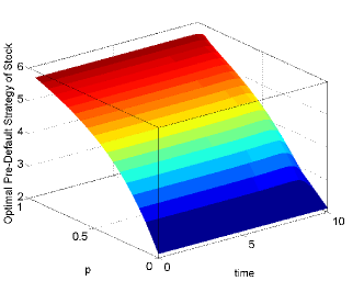
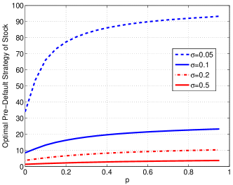
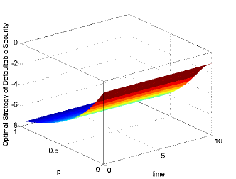
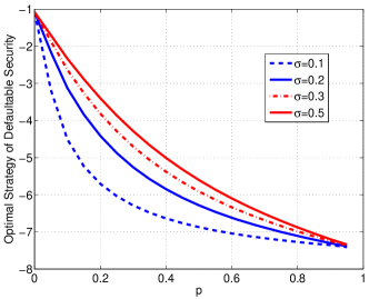
Figure 1 shows that the stock investment strategy is increasing in the filter probability of the hidden chain being in the first regime. This happens because under our parameter choices, the growth rate of the stock is higher in regime “1”, while the volatility stays unchanged. Consequently, if the filter estimate of being in the most profitable regime gets higher, the risk averse investor would prefer to shift a larger amount of wealth in the stock. On the other hand, as the probability of being in regime “1” increases, the risk averse investor shorts a higher amount of the defaultable security. This happens because the default intensity in regime “1” is the highest, and thus the risk averse investor wishing to decrease his exposure to default risk goes short in the vulnerable security. Notice also the key role played by the stock volatility $\sigma$. As the volatility gets lower, the investor shorts more units of the vulnerable security and invest the resulting proceeds in the stock security. Indeed, since the stock volatility is low while the default risk unchanged, the risk averse investor prefers to invest larger fraction of wealth in the stock security, and does so by raising cash via short-selling of the vulnerable security. The latter action also results in him having reduced exposure to credit risk. Since all model parameters depend on time only through the underlying hidden regime, investment strategies are not very sensitive to passage of time.

Figure 1: The top panels report the stock investment strategy. The bottom panels report the investment strategy in the vulnerable security. In the right panels, we set $t=0$.

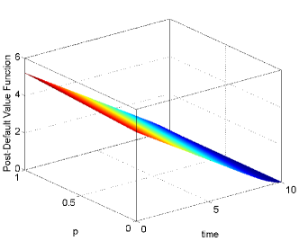
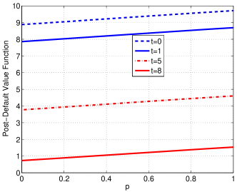
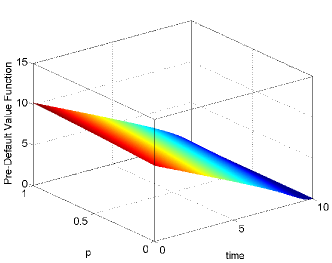
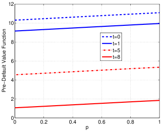
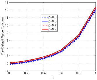
From figure 2, we can also see that both the pre-default and post-default value functions are decreasing in time, and increasing in the filter probability $p$. Moreover, as the filter probability of being in regime “1” increases, the investor extracts more utility given that he realizes higher gains by simultaneously shorting the vulnerable security and purchasing the stock security.

Figure 2: The pre-default and post-default value functions plotted versus time $t$ and filter probability $p$.

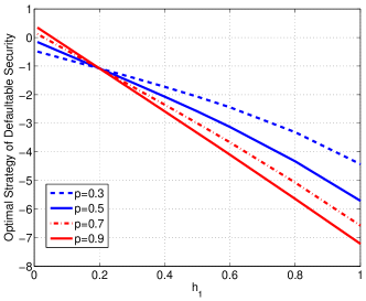
The investor increases the amount of shorted units of the vulnerable security if the filter probability of staying in the regime characterized by high default intensity gets larger. By contrast, if the filter probability of staying in the regime with low default intensity increases he takes higher credit risk exposure by purchasing more bond units. This is clearly illustrated in the left panel of figure 3. Moreover, when $h_{1}<h_{2}$ smaller amount of units of the vulnerable security are shorted if the probability $p$ of staying in the low risk regime gets higher. However, when the default intensity $h_{1}$ in regime “1” exceeds the default intensity $h_{2}$ in regime “2” ($h_{2}=0.2$), the opposite effect is observed. As $h_{1}$ gets higher, a larger amount of units of the vulnerable security are shorted if the filter probability of staying in regime “1” increases. We also notice that, ceteris paribus, the pre-default value function is increasing in $h_{1}$ for a fixed $p$ value, and also, for a given value of $h_{1}$ the pre-default value function increases in $p$.

Figure 3: The left panel reports the optimal investment strategy in the defaultable security. The right panel reports the pre-default value function. We set $t=0$.

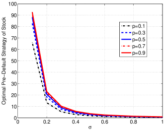
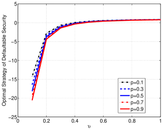
We next analyze the dependence of the optimal stock and vulnerable security investment strategies on the volatilities $\sigma$ and $\upsilon$. Figure 4 shows that when the stock volatility is low, the investor puts a large fraction of wealth in the stock security. This happens because the filter gain coming from receiving stock observations is the highest. Since observations are more informative, the risk averse investor deposits a larger fraction of wealth in the stock, especially if the filter probability of being in the high growth regime (regime “1” with $\mu_{1}=0.5$) is high. As the volatility gets larger, stock price observations become less informative leading the investor to decrease the wealth fraction invested in stock. When the volatility exceeds a certain threshold, regardless of the filter probability the investor always puts a small amount of wealth in the stock. We also notice that a similar role is played by the volatility $\upsilon$ of the defaultable security. From the right panel of figure 4, we notice that when $\upsilon$ is low, i.e. price observations of the vulnerable security are very informative, the investor wants to reduce more his exposure to default risk. Hence, he shorts more units of the vulnerable security especially if the filter probability of being in the highest credit risk regime (regime “1” with $h_{1}=0.05$) is large. This reflects the risk averse nature of the investor who dislikes default risk and uncertainty. As for the stock, when $\upsilon$ gets larger the investment strategy in the defaultable security becomes less sensitive to the filter probability and for large values of $\upsilon$ the investor may even find it optimal to purchase the defaultable security. This happens when the potential loss incurred by the investor when he is long credit and default occurs (hence making the vulnerable security worthless) is outweighed by the risk adjusted return resulting from holding the defaultable security.

We conclude by relating partial to full information settings. As price volatilities become smaller, the regime switching model becomes more observable. This is because price observations become more informative and allow the investor to build more accurate estimates of the regime in place. Consequently, the above analysis outlines the important role played by regime uncertainty in determining the optimal strategies of risk averse investors. Compared to the case of fully observed regimes studied in Capponi and Figueroa-López (2014), the presence of incomplete information induces the risk averse investor to decrease the wealth amount invested in the risky securities. As clearly illustrated in figure 4, when the price volatilities are sufficiently high ($\sigma\approx 0.8$ for the stock and $\upsilon\approx 0.6$ for the defaultable security), the investor deposits almost entire amount of wealth in the money market account.

Figure 4: The left panel reports the dependence of the optimal stock investment strategy on $\sigma$. The right panel reports the dependence of the optimal investment strategy in the vulnerable security on $\upsilon$. We set $t=0$. In the right panel, we set $h_{1}=0.05$ and $h_{2}=0.01$.

7 Conclusions

We have studied the optimal investment problem of a power investor in an economy consisting of a defaultable security, a stock, and a money market account. The price processes of these securities are assumed to have drift coefficients and default intensities modulated by a hidden Markov chain. We have reduced the partially observed stochastic control problem to a risk sensitive one, where the state is given by the filtered regime probabilities. The conditioning filtration, generated by the prices of the stock and of the defaultable security, and by the indicator of default occurrence, is driven both by a Brownian component and by a pure jump martingale. The filter has been used to derive the HJB partial differential equation corresponding to the risk sensitive control problem. We have split the latter into a pre-default and a post-default dynamic programming subproblem. The HJB PDE corresponding to the post-default value function can be transformed to a linear parabolic PDE, for which existence and uniqueness of a classical solution can be guaranteed. By contrast, the HJB PDE corresponding to the pre-default value function has exponential nonlinearity and quadratic gradient growth. We have provided a detailed mathematical analysis of such PDE and established the existence of a classical solution with $\mathcal{C}^{2,\alpha}_{P}$ regularity. We have then proven verification theorems establishing the correspondence between the PDE solutions and the value functions of the control problem. Our study has been complemented with a thorough numerical analysis illustrating the role of regime uncertainty, default risk, and price volatilities on the optimal allocation decisions and value functions.

Acknowledgments

The authors gratefully acknowledge two anonymous reviewers and Wolfgang Runggaldier for providing constructive and insightful comments which improved significantly the quality of the manuscript. Agostino Capponi would also like to thank Ramon Van Handel for very useful discussions and insights provided in the original model setup.

Appendix A Proofs related to Section 3

Lemma A.1.

Let

$$q_{t}^{i}=\mathbb{E}^{\hat{\mathbb{P}}}\left[L_{t}{\mathbf{1}_{\{X_{t}=e_{i}\}}}\bigg{|}\mathcal{G}_{t}^{I}\right].$$ (90)

Then, the dynamics of $(q_{t}^{i})_{t\geq{}0}$, $i=1,\dots,N$, under the measure $\hat{\mathbb{P}}$, is given by the following system of stochastic differential equations (SDE):

$$dq_{t}^{i} ={\sum_{\ell=1}^{N}\varpi_{\ell,i}(t)q^{\ell}_{t}}dt+q_{t}^{i}{\color[rgb]{0.00,0.00,0.00}Q^{\top}(t,e_{i},\pi_{t})}{\Sigma_{Y}}d\hat{W}_{t}+{q_{t^{-}}^{i}}(h_{i}-1)d\hat{\xi}_{t}-\gamma{\color[rgb]{0.00,0.00,0.00}\eta(t,e_{i},\pi_{t})}q_{t}^{i}dt{,}$$ (91)

$$q_{0}^{i} =p_{0}^{i}.$$

Proof.

Let us introduce the following notation

$$H_{t}^{i}:={\bf 1}_{\{X_{t}=e_{i}\}}.$$

Note that $X_{t}=(H^{1}_{t},\dots,H^{N}_{t})^{\top}$ and, from (1),

$$H^{i}_{t}=H_{0}^{i}+\int_{0}^{t}\sum_{\ell=1}^{N}\varpi_{\ell,i}(s)H^{\ell}_{s}ds+\color[rgb]{0.00,0.00,0.00}{\varphi_{i}(t)}.$$ (92)

From Eq. (28) and (22), we deduce that, under ${\hat{\mathbb{P}}}$,

$$dL_{t}=L_{t-}(h_{t}-1)d\hat{\xi}_{t}+L_{t}{\color[rgb]{0.00,0.00,0.00}Q^{\top}(t,X_{t},\pi_{t})}dY_{t}-L_{t}\gamma{\eta(t,X_{t},\pi_{t})}dt$$

which yields that

$$[L,{H^{i}}]_{t}=\int_{0}^{t}L_{s-}{\color[rgb]{0.00,0.00,0.00}Q^{\top}(s,X_{s},\pi_{s})}d[Y,{H^{i}}]_{s}+\int_{0}^{t}L_{s-}(h_{s}-1)d[\hat{\xi},{H^{i}}]_{s}.$$

As $(Y_{t})_{t\geq 0}$ and $(H_{t})_{t\geq 0}$ are independent of $(X_{t})_{t\geq 0}$ (and, hence, of $H^{i}$), under ${\hat{\mathbb{P}}}$ it holds (see also Wong and Hajek (1985)) that, ${\hat{\mathbb{P}}}$ almost surely,

$$[Y,{H^{i}}]_{s}=[\hat{\xi},{H^{i}}]_{s}=0,{\text{ for all }s\geq{}0.}$$

Thus, applying Itô’s formula, we obtain

$$L_{t}{H^{i}_{t}} = {H^{i}_{0}}+\int_{0}^{t}{H^{i}_{s^{-}}}dL_{s}+\int_{0}^{t}L_{s-}d{H_{s}^{i}}$$ (93)

$$= {H^{i}_{0}}+\int_{0}^{t}{H^{i}_{s}}L_{s}{\color[rgb]{0.00,0.00,0.00}Q^{\top}(s,X_{s},\pi_{s})}dY_{s}+\int_{0}^{t}{H^{i}_{s^{-}}L_{s^{-}}(h_{s^{-}}-1)}d\hat{\xi}_{s}$$

$$-\int_{0}^{t}{H^{i}_{s}}L_{s}\gamma{\color[rgb]{0.00,0.00,0.00}\eta(s,X_{s},\pi_{s})}ds+\int_{0}^{t}L_{s}{\sum_{\ell=1}^{N}\varpi_{\ell,i}(s)H^{\ell}_{s}}ds+\int_{0}^{t}L_{s-}d{{\color[rgb]{0.00,0.00,0.00}\varphi_{i}}(s)}$$

Since $({\color[rgb]{0.00,0.00,0.00}\varphi_{i}(t)})_{t\geq{}0}$ is a $((\mathcal{F}_{t}^{{X}})_{t\geq{}0},{\hat{\mathbb{P}}})$-martingale, and $\mathcal{G}_{T}^{I}$ is independent of $\mathcal{F}_{T}^{X}$ under ${\hat{\mathbb{P}}}$, we have that $\mathbb{E}^{{\hat{\mathbb{P}}}}\left[\int_{0}^{t}L_{s-}d{{\color[rgb]{0.00,0.00,0.00}\varphi_{i}(s)}}|{\mathcal{G}_{t}^{I}}\right]=0$. Therefore, taking $\mathcal{G}_{t}^{I}$ conditional expectations in Eq. (93), we obtain

$$\mathbb{E}^{{\hat{\mathbb{P}}}}\left[L_{t}{H^{i}_{t}|\mathcal{G}_{t}^{I}}\right] = 1+\int_{0}^{t}\mathbb{E}^{{\hat{\mathbb{P}}}}\left[L_{s}{H^{i}_{s}}{\color[rgb]{0.00,0.00,0.00}Q^{\top}(s,{e_{i}},\pi_{s})}|\mathcal{G}_{s}^{I}\right]dY_{s}+\int_{0}^{t}\mathbb{E}^{{\hat{\mathbb{P}}}}\left[L_{s^{-}}{H^{i}_{s^{-}}}({h_{s^{-}}}-1)|\mathcal{G}_{s}^{I}\right]d{\hat{\xi}_{s}}$$ (94)

$$-\int_{0}^{t}\mathbb{E}^{{\hat{\mathbb{P}}}}\left[{H^{i}_{s}}L_{s}\gamma{\color[rgb]{0.00,0.00,0.00}\eta(s,e_{i},\pi_{s})}|\mathcal{G}_{s}^{I}\right]ds+\int_{0}^{t}\mathbb{E}^{{\hat{\mathbb{P}}}}\left[{\sum_{\ell=1}^{N}\varpi_{\ell,i}(s)L_{s}H^{\ell}_{s}}|\mathcal{G}_{s}^{I}\right]ds,$$

where we have used that, if ${\varphi}_{t}$ is $\mathbb{G}$-predictable then (see, for instance, Wong and Hajek (1985), Ch. 7, Lemma 3.2)

$$\mathbb{E}^{{\hat{\mathbb{P}}}}\left[\int_{0}^{t}{\varphi}_{s}L_{s-}dY_{s}|\mathcal{G}_{t}^{I}\right] = \int_{0}^{t}\mathbb{E}^{{\hat{\mathbb{P}}}}\left[{\varphi}_{s}L_{s-}|\mathcal{G}_{s}^{I}\right]dY_{s}$$

$$\mathbb{E}^{{\hat{\mathbb{P}}}}\left[\int_{0}^{t}{\varphi}_{s}L_{s-}d\hat{\xi}_{s}|\mathcal{G}_{t}^{I}\right] = \int_{0}^{t}\mathbb{E}^{{\hat{\mathbb{P}}}}\left[{\varphi}_{s}L_{s-}|\mathcal{G}_{s}^{I}\right]d\hat{\xi}_{s}$$

$$\mathbb{E}^{{\hat{\mathbb{P}}}}\left[\int_{0}^{t}{\varphi}_{s}L_{s-}ds|\mathcal{G}_{t}^{I}\right] = \int_{0}^{t}\mathbb{E}^{{\hat{\mathbb{P}}}}\left[{\varphi}_{s}L_{s-}|\mathcal{G}_{s}^{I}\right]ds$$

Observing that under ${\hat{\mathbb{P}}}$ $dY_{t}={\Sigma_{Y}}d\hat{W}_{t}$, using that $Q(t,{e_{i}},\pi_{t})$ and $\eta(t,e_{i},\pi_{t})$ are $(\mathcal{G}_{t}^{I})_{t\geq{}0}$ adapted, and that the Markov-chain generator $A(t)$ is deterministic, we obtain Eq. (A.1) upon taking the differential of Eq. (94). ∎

Lemma A.2.

The following identities hold

$$q_{t}^{i} = \hat{L}_{t}p_{t}^{i}$$ (95)

$$p_{t}^{i} = \frac{q_{t}^{i}}{\sum_{j=1}^{N}q_{t}^{j}}$$ (96)

where $q_{t}^{i}$, $\hat{L}_{t}$, and $p_{t}^{i}$ are defined, respectively, by (90), (35), and (32).

Proof.

We start establishing the relation (95) by comparing the dynamics of $q_{t}^{i}$ and of ${\hat{L}_{t}p_{t}^{i}}$. The dynamics of $q_{t}^{i}$ is known from Lemma A.1 and given in Eq. (A.1). Next, we derive the dynamics of $\hat{L}_{t}p_{t}^{i}$. We have

$$d(\hat{L}_{t}p_{t}^{i})=\hat{L}_{{t^{-}}}dp_{t}^{i}+p_{{t^{-}}}^{i}d\hat{L}_{t}+d\left[\hat{L},p^{i}\right]_{t}.$$

From Eq. (36) and (34), we obtain

$$d\left[\hat{L},p^{i}\right]_{t} =p_{t}^{i}\hat{L}_{t}{\color[rgb]{0.00,0.00,0.00}\hat{\vartheta}^{\top}(t,p_{t})}\Sigma_{Y}\Sigma_{Y}^{-1}\left({\color[rgb]{0.00,0.00,0.00}\vartheta(t,e_{i})-{\color[rgb]{0.00,0.00,0.00}\hat{\vartheta}}(t,p_{t})}\right)dt+p_{t}^{i}\hat{L}_{t}\gamma\pi_{t}^{\top}\left({\color[rgb]{0.00,0.00,0.00}\vartheta(t,e_{i})-{\color[rgb]{0.00,0.00,0.00}\hat{\vartheta}}(t,p_{t})}\right)dt$$

$$\quad+\left(\hat{h}_{{t^{-}}}-1\right)\frac{h_{i}-\hat{h}_{{t^{-}}}}{\hat{h}_{{t^{-}}}}\hat{L}_{{t^{-}}}p_{{t^{-}}}^{i}dH_{t}.$$ (97)

Using the above equations, along with (34), we obtain

$$d\left(\hat{L}_{t}p_{t}^{i}\right) = \hat{L}_{t}\left(\sum_{\ell=1}^{N}\varpi_{\ell,i}(t)p^{\ell}_{t}dt\right)+\hat{L}_{t}p_{t}^{i}\left({\color[rgb]{0.00,0.00,0.00}\vartheta^{\top}(t,e_{i})-{\color[rgb]{0.00,0.00,0.00}\hat{\vartheta}}^{\top}(t,p_{t})}\right)\left(\Sigma_{Y}\Sigma^{\top}_{Y}\right)^{-1}\left(dY_{t}-{\color[rgb]{0.00,0.00,0.00}{\color[rgb]{0.00,0.00,0.00}\hat{\vartheta}(t,p_{t})}}dt\right)$$

$$+ \hat{L}_{{t^{-}}}p_{{t^{-}}}^{i}\frac{h_{i}-\hat{h}_{{t^{-}}}}{\hat{h}_{{t^{-}}}}\left(dH_{t}-\hat{h}_{{t^{-}}}{\bar{H}_{t^{-}}}dt\right)+p_{t}^{i}\hat{L}_{t}{\color[rgb]{0.00,0.00,0.00}\hat{Q}^{\top}(t,p_{t},\pi_{t})}dY_{t}-p_{t}^{i}{\hat{L}_{t}\gamma{\color[rgb]{0.00,0.00,0.00}\hat{\eta}(t,p_{t},\pi_{t})}}dt$$

$$+ p_{{t^{-}}}^{i}\hat{L}_{{t^{-}}}(\hat{h}_{{t^{-}}}-1)(dH_{t}-{\color[rgb]{0.00,0.00,0.00}\bar{H}_{t^{-}}}dt)+(\hat{h}_{{t^{-}}}-1)\frac{h_{i}-\hat{h}_{{t^{-}}}}{\hat{h}_{{t^{-}}}}\hat{L}_{{t^{-}}}p_{{t^{-}}}^{i}dH_{t}$$

$$+ p_{t}^{i}\hat{L}_{t}{\color[rgb]{0.00,0.00,0.00}\hat{\vartheta}^{\top}(t,p_{t})}\left(\Sigma_{Y}\Sigma_{Y}^{\top}\right)^{-1}{\left(\vartheta(t,e_{i})-\color[rgb]{0.00,0.00,0.00}{\hat{\vartheta}}(t,p_{t})\right)dt}+\gamma p_{t}^{i}\hat{L}_{t}\pi_{t}^{\top}\left({\color[rgb]{0.00,0.00,0.00}\vartheta(t,e_{i})-{\color[rgb]{0.00,0.00,0.00}\hat{\vartheta}}(t,p_{t})}\right)dt.$$

Next, observe that

$$\hat{L}_{t}p_{t}^{i}\left({\color[rgb]{0.00,0.00,0.00}\vartheta^{\top}(t,e_{i})-{\color[rgb]{0.00,0.00,0.00}\hat{\vartheta}}^{\top}(t,p_{t})}\right)(\Sigma_{Y}\Sigma_{Y}^{\top})^{-1}(dY_{t}-{\color[rgb]{0.00,0.00,0.00}\hat{\vartheta}}(t,p_{t})dt)+p_{t}^{i}\hat{L}_{t}{\color[rgb]{0.00,0.00,0.00}\hat{Q}}^{\top}(t,p_{t},\pi_{t})dY_{t} =$$

$$\hat{L}_{t}p_{t}^{i}{\color[rgb]{0.00,0.00,0.00}Q^{\top}(t,e_{i},\pi_{t})}dY_{t}-\hat{L}_{t}p_{t}^{i}\left({\color[rgb]{0.00,0.00,0.00}\vartheta^{\top}(t,e_{i})-{\color[rgb]{0.00,0.00,0.00}\hat{\vartheta}}^{\top}(t,p_{t})}\right)(\Sigma_{Y}\Sigma_{Y}^{\top})^{-1}{\color[rgb]{0.00,0.00,0.00}\hat{\vartheta}}(t,p_{t})dt$$ (99)

Moreover,

$$\eta(t,e_{i},\pi_{t})-{\color[rgb]{0.00,0.00,0.00}\hat{\eta}}(t,p_{t},\pi_{t})=\pi_{t}^{\top}\left({\color[rgb]{0.00,0.00,0.00}\hat{\vartheta}(t,p_{t})}-\vartheta(t,e_{i})\right).$$ (100)

Using relations (99), and (100), along with straightforward simplifications, we may simplify Eq. (A) to

$$d(\hat{L}_{t}p_{t}^{i})=\left(\sum_{\ell=1}^{N}\varpi_{\ell,i}(t)\hat{L}_{t}p^{\ell}_{t}dt\right)+\hat{L}_{t}p_{t}^{i}{\color[rgb]{0.00,0.00,0.00}Q^{\top}(t,e_{i},\pi_{t})}dY_{t}-\gamma\hat{L}_{t}p_{t}^{i}{\color[rgb]{0.00,0.00,0.00}\eta(t,e_{i},\pi_{t})}dt+\hat{L}_{{t^{-}}}p_{{t^{-}}}^{i}(h_{i}-1)d\hat{\xi}_{t}.$$ (101)

Using that $dY_{t}=\Sigma_{Y}d\hat{W}_{t}$, we have that the equality (95) holds via a direct comparison of equations (101) and (A.1).

Next, we establish (96). Using Eq. (95) and that $\sum_{i=1}^{N}p_{t}^{i}=1$, we deduce that

$$d\left(\sum_{i=1}^{N}q_{t}^{i}\right)=d\left(\sum_{i=1}^{N}\hat{L}_{t}p_{t}^{i}\right)=d\hat{L}_{t}$$

hence obtaining that $\sum_{i=1}^{N}q_{t}^{i}=\hat{L}_{t}$. Using again (95), this gives

$$p_{t}^{i}=\frac{q_{t}^{i}}{\hat{L}_{t}}=\frac{q_{t}^{i}}{\sum_{j=1}^{N}q_{t}^{j}}$$

This completes the proof. ∎

Proof of Proposition 3.3.

Proof.

Using Eq. (27), (90), and the relation (95) established in Lemma A.2 , we have that

$$J(v,\pi,T) = \frac{1}{\gamma}\mathbb{E}^{\mathbb{P}}\left[V_{T}^{\gamma}\right]=\frac{v^{\gamma}}{\gamma}\mathbb{E}^{\hat{\mathbb{P}}}\left[L_{T}\right]=\frac{v^{\gamma}}{\gamma}\mathbb{E}^{\hat{\mathbb{P}}}\left[\mathbb{E}^{\hat{\mathbb{P}}}\left[L_{T}\big{|}\mathcal{G}_{T}^{I}\right]\right]$$

$$= \frac{v^{\gamma}}{\gamma}\sum_{i=1}^{N}\mathbb{E}^{\hat{\mathbb{P}}}\left[\mathbb{E}^{\hat{\mathbb{P}}}\left[L_{T}\mathbf{1}_{{\{X_{T}=e_{i}\}}}\big{|}\mathcal{G}_{T}^{I}\right]\right]=\frac{v^{\gamma}}{\gamma}{\sum_{i=1}^{N}\mathbb{E}^{\hat{\mathbb{P}}}\left[q_{T}^{i}\right]}$$

$$= \frac{v^{\gamma}}{\gamma}\sum_{i=1}^{N}\mathbb{E}^{\hat{\mathbb{P}}}\left[\hat{L}_{T}p_{T}^{i}\right]=\frac{v^{\gamma}}{\gamma}\mathbb{E}^{\hat{\mathbb{P}}}\left[\hat{L}_{T}\right],$$

thus proving the statement. ∎

Appendix B Proofs related to Section 5

We start with a Lemma, which will be needed in the section where the verification theorem is proven.

Lemma B.1.

For any $T>0$ and $i\in\{1,\dots,N\}$, it holds that

1. ${\mathbb{P}}\left(p^{i}_{t}>0,\,\textrm{for\ all }\ t\in[0,T)\right)=1$.

2. ${\mathbb{P}}\left(p^{i}_{t}<1,\,\textrm{for\ all }\ t\in[0,T)\right)=1$.

Proof.

Define $\varsigma=\inf\{t:p^{i}_{t}=0\}\wedge T$. If $p^{i}_{t}$ can hit zero, then $\mathbb{P}(p^{i}_{\varsigma}=0)>0$. Recall that $p_{t}^{i}=\frac{q_{t}^{i}}{\sum_{j}q_{t}^{j}}$ from Eq. (96), hence $p_{\varsigma}^{i}=\frac{q_{\varsigma}^{i}}{\sum_{j}q_{\varsigma}^{j}}$, where the equality

$$q_{\varsigma}^{i}=\mathbb{E}^{\hat{\mathbb{P}}}\left[L_{\varsigma}\mathbf{1}_{X_{\varsigma}=e_{i}}\big{|}\mathcal{G}_{\varsigma}^{I}\right]$$

is true by the optional projection property, see Rogers and Williams (2006). Define the two dimensional (observed) log-price process $Y_{t}=(\log(S_{t}),{\log(P_{t})})^{\top}$. As $q_{\varsigma}^{i}=\mathbb{E}^{\hat{\mathbb{P}}}\left[L_{\varsigma}1_{X_{\varsigma}=e_{i}}|\mathcal{G}_{\varsigma}^{I}\right]$, and using that $L_{\varsigma}>0$, we can choose a modification $g(Y,H,X_{\varsigma})$ of $\mathbb{E}^{{\hat{\mathbb{P}}}}\left[L_{\varsigma}|\mathcal{G}_{\varsigma}^{I},X_{\varsigma}\right]$ such that $g>0$, and, for each $e_{i}$, $g(Y,H,{e_{i}})$ is $G_{\varsigma}^{I}$-measurable. By the tower property

$$q_{\varsigma}^{i}=\mathbb{E}^{\hat{\mathbb{P}}}[g(Y,H,X_{\varsigma})\mathbf{1}_{X_{\varsigma}=e_{i}}|\mathcal{G}_{\varsigma}^{I}]=g(Y,H,e_{i})\hat{\mathbb{P}}(X_{\varsigma}=e_{i}|\mathcal{G}_{\varsigma}^{I})=g(Y,H,e_{i})\mathbb{P}(X_{t}=e_{i})\big{|}_{t=\varsigma},$$

where the first equality follows because $\varsigma$ is $\mathcal{G}^{I}_{\varsigma}$-measurable and the last two equalities because $X$ is independent of $\mathcal{G}^{I}$ under $\hat{\mathbb{P}}$. As $\mathbb{P}(X_{t}=e_{i})>0$ and $g>0$, we get that $q_{\varsigma}^{i}>0$ a.s, which contradicts that $\mathbb{P}(p_{\varsigma}^{i}=0)>0$. This proves the first statement in the Lemma. Next, we notice that

$$\mathbb{P}\left(p^{i}_{t}=0,\,\textrm{for\ some }\ t\in[0,T)\right)=1-\mathbb{P}\left(p^{i}_{t}>0,\,\textrm{for\ all }\ t\in[0,T)\right)=0,$$

where the last equality follows from the first statement. This immediately yields the second statement.∎

Proof of Eq. (81)

Proof.

Let us first analyze the first term in the sup of Eq. (79), i.e. ${\color[rgb]{0.00,0.00,0.00}\beta_{\gamma}^{\top}}\nabla_{\widetilde{p}}w$. For brevity, we use $\beta_{\varpi}:=\beta_{\varpi}(t,\widetilde{p},0)$. By definition of ${\color[rgb]{0.00,0.00,0.00}\beta_{\gamma}}$, and using the maximizer $\pi_{t}:=\pi^{*}_{t}$ in (80), we have

$${{\color[rgb]{0.00,0.00,0.00}\beta^{\top}_{\gamma}}={\color[rgb]{0.00,0.00,0.00}\beta_{\varpi}^{\top}}+\gamma{\pi^{\top}}\Sigma_{Y}\bar{\kappa}^{\top}} = {\color[rgb]{0.00,0.00,0.00}\beta_{\varpi}}^{\top}+\frac{\gamma}{1-\gamma}\left(\Sigma_{Y}\bar{\kappa}^{\top}(\nabla_{\widetilde{p}}\bar{w})^{\top}-\Upsilon\right)^{\top}(\Sigma_{Y}^{\top}\Sigma_{Y})^{-1}\Sigma_{Y}\bar{\kappa}^{\top}$$ (102)

$$= {\color[rgb]{0.00,0.00,0.00}\beta_{\varpi}^{\top}}+\frac{\gamma}{1-\gamma}(\nabla_{\widetilde{p}}\bar{w})\bar{\kappa}\Sigma_{Y}^{\top}(\Sigma_{Y}^{\top}\Sigma_{Y})^{-1}\Sigma_{Y}\bar{\kappa}^{\top}-\frac{\gamma}{1-\gamma}\Upsilon^{\top}(\Sigma_{Y}^{\top}\Sigma_{Y})^{-1}\Sigma_{Y}\bar{\kappa}^{\top}$$

Further, again using the expression for $\pi=\pi^{*}$, the second term in the sup is equal to

$${-}\gamma\pi^{\top}\Upsilon = {-}\frac{\gamma}{1-\gamma}\left(-\Upsilon+\Sigma_{Y}\bar{\kappa}^{\top}{(\nabla_{\widetilde{p}}\bar{w})^{\top}}\right)^{\top}(\Sigma_{Y}^{\top}\Sigma_{Y})^{-1}\Upsilon$$ (103)

$$= \frac{\gamma}{1-\gamma}\Upsilon^{\top}(\Sigma_{Y}^{\top}\Sigma_{Y})^{-1}\Upsilon\,{-}\,\frac{\gamma}{1-\gamma}{(\nabla_{\widetilde{p}}\bar{w})}\bar{\kappa}\Sigma_{Y}^{\top}(\Sigma_{Y}^{\top}\Sigma_{Y})^{-1}{\Upsilon.}$$

The third term in the sup may be simplified as

$$-\frac{1}{2}\frac{\gamma}{1-\gamma}\left(-\Upsilon+\Sigma_{Y}\bar{\kappa}^{\top}{(\nabla_{\widetilde{p}}\bar{w})^{\top}}\right)^{\top}(\Sigma_{Y}^{\top}\Sigma_{Y})^{-1}(-\Upsilon+\Sigma_{Y}\bar{\kappa}^{\top}{(\nabla_{\widetilde{p}}\bar{w})^{\top}})=$$

$$\quad-\frac{1}{2}\frac{\gamma}{1-\gamma}\Upsilon^{\top}(\Sigma_{Y}^{\top}\Sigma_{Y})^{-1}\Upsilon+\frac{1}{2}\frac{\gamma}{1-\gamma}\Upsilon^{\top}(\Sigma_{Y}^{\top}\Sigma_{Y})^{-1}\Sigma_{Y}\bar{\kappa}^{\top}{(\nabla_{\widetilde{p}}\bar{w})^{\top}}$$

$$\quad+\frac{1}{2}\frac{\gamma}{1-\gamma}{(\nabla_{\widetilde{p}}\bar{w})}\bar{\kappa}\Sigma_{Y}^{\top}(\Sigma_{Y}^{\top}\Sigma_{Y})^{-1}\Upsilon-\frac{1}{2}\frac{\gamma}{1-\gamma}{(\nabla_{\widetilde{p}}\bar{w})}\bar{\kappa}\Sigma_{Y}^{\top}(\Sigma_{Y}^{\top}\Sigma_{Y})^{-1}\Sigma_{Y}\bar{\kappa}^{\top}{(\nabla_{\widetilde{p}}\bar{w})^{\top}.}$$ (104)

Using Eq. (102), (103), and (104), we obtain that

$$\sup_{\pi}\bigg{\{}{\color[rgb]{0.00,0.00,0.00}\beta_{\gamma}^{\top}}{(\nabla_{\widetilde{p}}\bar{w})^{\top}}-\gamma\pi_{t}^{\top}\Upsilon-\frac{1}{2}\gamma(1-\gamma)\pi_{t}^{\top}\Sigma^{\top}_{Y}\Sigma_{Y}\pi_{t}\bigg{\}}=$$

$${\color[rgb]{0.00,0.00,0.00}\beta_{\varpi}^{\top}}(\nabla_{\widetilde{p}}\bar{w})^{\top}+\frac{1}{2}\frac{\gamma}{1-\gamma}{(\nabla_{\widetilde{p}}\bar{w})}\bar{\kappa}\Sigma_{Y}^{\top}(\Sigma_{Y}^{\top}\Sigma_{Y})^{-1}\Sigma_{Y}\bar{\kappa}^{\top}{(\nabla_{\widetilde{p}}\bar{w})^{\top}}+\frac{1}{2}\frac{\gamma}{1-\gamma}\Upsilon^{\top}(\Sigma_{Y}^{\top}\Sigma_{Y})^{-1}\Upsilon{-\frac{\gamma}{1-\gamma}(\nabla_{\widetilde{p}}\bar{w})}\bar{\kappa}\Sigma_{Y}^{-1}\Upsilon,$$

and therefore, after re-arrangement, we obtain Eq. (81). ∎

Proof of Theorem 5.3.

Proof.

In order to ease the notational burden, throughout the proof we will write $\widetilde{p}$ for $\widetilde{p}^{\circ}$, $\widetilde{p}_{s}$ for $\widetilde{p}^{t}_{s}$, $\pi$ for $\pi^{t}$, $\widetilde{\mathbb{P}}$ for ${\widetilde{\mathbb{P}}^{t}}$, $\mathbb{P}$ for ${\mathbb{P}^{t}}$, $\widetilde{W}$ for $\widetilde{W}^{t}$, $X$ for $X^{t}$, and $\mathcal{G}_{s}^{I}$ for $\mathcal{G}_{s}^{t,I}$. Let us first remark that

$${\mathbb{P}}\left(\widetilde{p}_{s}\in\widetilde{\Delta}_{N-1},\,t\leq s\leq T\right)=1.$$ (105)

Indeed, set $\widetilde{p}^{N}_{s}=1-\sum_{j=1}^{N-1}\widetilde{p}^{j}_{s}$ and recall from Remark 3.4 that the process $\widetilde{p}_{s}^{i}$ is given by

$${\widetilde{p}_{s}^{i}:={{\mathbb{P}}}\left(X_{s}=e_{i}\big{|}\mathcal{G}_{s}^{I}\right),\qquad(t\leq{}s\leq{}T,\;i=1,\dots,N).}$$ (106)

Therefore, using Lemma B.1, we deduce that all the $\widetilde{p}^{i}$, with $i=1,\dots,N$, remain positive in $[t,T]$, a.s., and, hence, (105) is satisfied.

Next, we prove that the feedback trading strategy $\widetilde{\pi}_{s}:=(\widetilde{\pi}^{S}_{s},\widetilde{\pi}^{P}_{s})^{\top}$, $\widetilde{\pi}^{P}_{s}:=0$, is admissible; i.e.,

$$\mathbb{E}^{\mathbb{P}}\left[\exp\left(\frac{\sigma^{2}\gamma^{2}}{2}\int_{t}^{T}\left(\widetilde{\pi}^{S}\left(s,\widetilde{p}_{s}\right)\right)^{2}ds\right)\right]<\infty.$$ (107)

We have that (107) follows from Eq. (105) and the fact that $(\widetilde{\pi}^{S}(s,\widetilde{p}))^{2}$ is uniformly bounded on $[0,T]\times\widetilde{\Delta}_{N-1}$. To see the latter property, note that

$$\sup_{(s,\widetilde{p})\in[0,T]\times\widetilde{\Delta}_{N-1}}\left(\widetilde{\pi}^{S}(s,\widetilde{p})\right)^{2}\leq\frac{2}{\sigma^{4}(1-\gamma)^{2}}\sup_{(s,\widetilde{p})\in[0,T]\times\widetilde{\Delta}_{N-1}}\left(\widetilde{\mu}(\widetilde{p})-r\right)^{2}+\frac{2}{\sigma^{{\color[rgb]{0.00,0.00,0.00}2}}(1-\gamma)^{2}}\sup_{(s,\widetilde{p})\in[0,T]\times\widetilde{\Delta}_{N-1}}\left({\nabla_{\widetilde{p}}\underline{w}(s,\widetilde{p})\underline{\kappa}(\widetilde{p})}\right)^{2}.$$

The first term on the right hand side is clearly bounded since $|\widetilde{\mu}(\widetilde{p})|\leq\max_{i}|\mu_{i}|$ for any $\widetilde{p}\in\widetilde{\Delta}_{N-1}$. For the second term, using the definition of $\underline{\kappa}$ given in Eq. (71), we have

$$\sup_{(s,\widetilde{p})\in[0,T]\times\widetilde{\Delta}_{N-1}}\left({\nabla_{\widetilde{p}}\underline{w}(s,\widetilde{p})\underline{\kappa}(\widetilde{p})}\right)^{2}=\frac{1}{\sigma^{2}}\sup_{(s,\widetilde{p})\in[0,T]\times\widetilde{\Delta}_{N-1}}\left(\sum_{j=1}^{N-1}\partial_{\widetilde{p}^{j}}\underline{w}(s,\widetilde{p})\widetilde{p}^{j}\left(\mu_{j}-\sum_{i=1}^{N}\mu_{i}\widetilde{p}^{i}\right)\right)^{2},$$ (108)

where $\widetilde{p}^{N}:=1-\sum_{i=1}^{N-1}\widetilde{p}^{i}$. The last expression is bounded since each $\partial_{\widetilde{p}^{j}}\underline{w}(s,\widetilde{p})$ is bounded on $[0,T]\times\widetilde{\Delta}_{N-1}$ in view of Lemma 5.1 and Remark 5.2, where it is shown $\mathcal{C}_{P}^{2,\alpha}$ regularity for $\underline{w}(s,\widetilde{p})$, hence bounded first and second order space derivatives on $\widetilde{\Delta}_{N-1}$.

Now, fix an arbitrary feedback control $\pi_{s}^{S}:=\pi^{S}(s,\widetilde{p}_{s})$ such that $(\pi^{S},\pi^{P})\in{\mathcal{A}}(t,T;\widetilde{p},1)$, where $\pi^{P}_{s}\equiv 0$ and ${\mathcal{A}}(t,T;\widetilde{p},1)$ is defined as in Definition 4.1, and define the process

$$M_{s}^{\pi^{S}}:=e^{-\gamma\int_{t}^{s}\underline{\eta}(u,\widetilde{p}_{u},\pi^{S}_{u})du}e^{\underline{w}(s,\widetilde{p}_{s})},\qquad(t\leq{}s\leq{}T),$$

where

$$\underline{\eta}(u,\widetilde{p},\pi^{S})={\eta}(u,\widetilde{p},(\pi^{S},0)^{\top})=-r+{\pi^{S}}(r-\widetilde{\mu}(\widetilde{p}))+\frac{1-\gamma}{2}\sigma^{2}\left(\pi^{S}\right)^{2}.$$ (109)

In what follows, we write for simplicity $M^{\pi}$ for $M^{\pi^{S}}$ and $\pi$ for $\pi^{S}$. Note that the process $\{M^{\pi}_{s}\}_{t\leq{}s\leq{}T}$ is uniformly bounded. Indeed, (109) is convex in $\pi^{S}$ and by minimizing it over $\pi^{S}$, it follows that, for any $\widetilde{p}\in\widetilde{\Delta}_{N-1}$,

$$-\underline{\eta}(t,\widetilde{p},\pi)\leq r+\frac{(\widetilde{\mu}(\widetilde{p})-r)^{2}}{2(1-\gamma)\sigma^{2}}\leq r+\frac{(\max_{i}\mu_{i}^{2}+r^{2})}{(1-\gamma)\sigma^{2}}<{\infty}.$$

Therefore, since $\underline{w}\in C([0,T]\times\widetilde{\Delta}_{N-1})$, there exists a constant $K<\infty$ for which

$$M_{s}^{\pi}=e^{-\gamma\int_{t}^{s}\underline{\eta}(u,\widetilde{p}_{u},\pi_{u})du}e^{\underline{w}(s,\widetilde{p}_{s})}\leq Ke^{\gamma\|\underline{\eta}\|_{\infty}(T-t)}=:A<\infty.$$ (110)

We prove the result through the following steps:

(i) Define the process $\mathcal{Y}_{s}=e^{\underline{w}(s,\widetilde{p}_{s})}$. By Itô’s formula and the generator formula (56) with $f(s,\widetilde{p})=e^{\underline{w}(s,\widetilde{p})}$,

$$M_{s}^{\pi} =M_{t}^{\pi}+\int_{t}^{s}e^{-\gamma\int_{t}^{u}\underline{\eta}(r,\widetilde{p}_{r},\pi_{r})dr}d\mathcal{Y}_{u}-\gamma\int_{t}^{s}\underline{\eta}(u,\widetilde{p}_{u},\pi_{u})e^{-\gamma\int_{t}^{u}\underline{\eta}(r,\widetilde{p}_{r},\pi_{r})dr}\mathcal{Y}_{u}du$$

$$=M_{t}^{\pi}+\int_{t}^{s}M_{u}^{\pi}\left({\frac{\partial\underline{w}}{\partial u}}+\frac{1}{2}\text{tr}(\underline{\kappa}\underline{\kappa}^{\top}D^{2}\underline{w})+\frac{1}{2}{(\nabla_{\widetilde{p}}\underline{w})\underline{\kappa}\underline{\kappa}^{\top}(\nabla_{\widetilde{p}}\underline{w})^{\top}}+{(\nabla_{\widetilde{p}}\underline{w})\underline{\beta}_{\gamma}}-\gamma\underline{\eta}\right)du+\int_{t}^{s}M_{u}^{\pi}\nabla_{\widetilde{p}}\underline{w}\,\underline{\kappa}\,d{\widetilde{W}}^{(1)}_{u}.$$

Using the expression of $\underline{\eta}$ in (109) and some rearrangement, we may write $M^{\pi}$ as

$$M_{s}^{\pi}=M_{t}^{\pi}+\int_{t}^{s}M_{u}^{\pi}R(u,\widetilde{p}_{u},\pi_{u})du+\int_{t}^{s}M_{u}^{\pi}\nabla_{\widetilde{p}}\underline{w}\,\underline{\kappa}\,d{\widetilde{W}}^{(1)}_{u}$$

with

$$R(u,\widetilde{p},\pi)={\underline{w}}_{u}+\frac{1}{2}\text{tr}(\underline{\kappa}\underline{\kappa}^{\top}D^{2}\underline{w})+\frac{1}{2}{(\nabla_{\widetilde{p}}\underline{w})\underline{\kappa}\underline{\kappa}^{\top}(\nabla_{\widetilde{p}}\underline{w})^{\top}}+\gamma r+{(\nabla_{\widetilde{p}}w)\underline{\beta}_{\gamma}}-\gamma\pi(r-\widetilde{\mu}(\widetilde{p}))-\frac{{\sigma^{2}}}{2}\gamma(1-\gamma)\pi^{2}.$$ (111)

Clearly, $R(u,\widetilde{p},\pi)$ is a concave function in $\pi$ since $R_{\pi\pi}=-\sigma^{2}\gamma(1-\gamma)<0$. If we maximize $R(u,\widetilde{p},\pi)$ as a function of $\pi$ for each $(u,\widetilde{p})$, we find that the optimum is given by (75). Upon substituting (75) into (111), we get that

$$R(u,\widetilde{p},\pi) \leq R(u,\widetilde{p},{\widetilde{\pi}^{S}(u,\widetilde{p})})=\underline{w}_{u}+\frac{1}{2}\text{tr}(\underline{\kappa}\underline{\kappa}^{\top}D^{2}\underline{w})+\frac{1}{2(1-\gamma)}{(\nabla_{\widetilde{p}}\underline{w})\underline{\kappa}\,\underline{\kappa}^{\top}(\nabla_{\widetilde{p}}\underline{w})^{\top}}+{(\nabla_{\widetilde{p}}\underline{w})\underline{\Phi}}+\underline{\Psi}=0,$$

where the last equality follows from Eq. (73). Therefore, we get the inequality

$${\mathbb{E}^{\widetilde{\mathbb{P}}}}\left[M^{\pi}_{T}\right] \leq M_{t}^{\pi}+{\mathbb{E}^{\widetilde{\mathbb{P}}}}\left[\int_{t}^{T}M_{u}^{\pi}\nabla_{\widetilde{p}}\underline{w}\,\underline{\kappa}\,d{\widetilde{W}}^{(1)}_{u}\right],$$

with equality if $\pi=\widetilde{\pi}^{S}$. From (71), it is easy to check that $\sup_{\widetilde{p}\in\widetilde{\Delta}_{N-1}}\|\underline{\kappa}(\widetilde{p})\|^{2}\leq 2\max_{i}\{\mu_{i}\}/\sigma$. Then, since the partial derivatives $\partial_{\widetilde{p}^{j}}\underline{w}(s,\widetilde{p})$ are uniformly bounded on $[0,T]\times\widetilde{\Delta}_{N-1}$ (see also the argument after Eq. (108)), (110) implies that

$${\sup_{t\leq u\leq T}\left|M_{u}^{\pi}\nabla_{\widetilde{p}}\underline{w}\,\underline{\kappa}\right|^{2}\leq A\sup_{t\leq u\leq T}\|\underline{\kappa}(\widetilde{p}_{u})\|^{2}\sup_{t\leq u\leq T}\|\nabla_{\widetilde{p}}\underline{w}(u,\widetilde{p}_{u})\|^{2}\leq B},$$

for some non-random constant $B<\infty$. We conclude that

$$\mathbb{E}^{\widetilde{\mathbb{P}}}\left[M^{\pi}_{T}\right]\leq M_{t}^{\pi}=e^{\underline{w}(t,\widetilde{p}_{t})}=e^{\underline{w}(t,\widetilde{p})},$$ (112)

with equality if $\pi=\widetilde{\pi}^{S}$.

(ii) For simplicity, let us write $\widetilde{\pi}_{s}:=\widetilde{\pi}^{S}(s,\widetilde{p}_{s})$. First, note that from the fact that we have equality in (112) when $\pi=\widetilde{\pi}$,

$${e^{\underline{w}(t,\widetilde{p})}=\mathbb{E}^{\widetilde{\mathbb{P}}}\left[M^{\widetilde{\pi}}_{T}\right]=\mathbb{E}^{\widetilde{\mathbb{P}}}\left[e^{-\gamma\int_{t}^{T}\underline{\eta}(u,\widetilde{p}_{u},\widetilde{\pi}_{u})du}e^{\underline{w}(T,\widetilde{p}_{T})}\right]=\mathbb{E}^{\widetilde{\mathbb{P}}}\left[e^{-\gamma\int_{t}^{T}\underline{\eta}(u,\widetilde{p}_{u},\widetilde{\pi}_{u})du}\right]}.$$ (113)

Similarly, for every feedback control $\pi_{s}=\pi(s,\widetilde{p}_{s})$ such that $(\pi,0)\in\mathcal{A}(t,T;\widetilde{p},1)$,

$${{\mathbb{E}^{\widetilde{\mathbb{P}}}\left[e^{-\gamma\int_{t}^{T}\underline{\eta}(u,\widetilde{p}_{u},\pi_{u})du}\right]=\mathbb{E}^{\widetilde{\mathbb{P}}}\left[M^{\pi}_{T}\right]\leq e^{\underline{w}(t,\widetilde{p})}=\mathbb{E}^{{\widetilde{\mathbb{P}}}}\left[e^{-\gamma\int_{t}^{T}\underline{\eta}(u,\widetilde{p}_{u},\widetilde{\pi}_{u})du}\right],}}$$

where the inequality in the previous equation comes from (112) and the last equality therein follows from (113). The previous relationships show the optimality of $\widetilde{\pi}$ and prove the assertions (1) and (2). ∎

Proof of Theorem 5.4.

Proof.

For brevity, define the operator

$$\mathcal{B}=\partial_{t}+\frac{1}{2}\text{tr}\left(\bar{\kappa}\bar{\kappa}^{\top}D^{2}\right)+\nabla_{\widetilde{p}}\bar{\Phi}$$

and denote by

$$H(t,\widetilde{p},u)=-\widetilde{h}({\widetilde{p}})e^{\underline{w}\left(t,\frac{1}{\widetilde{h}({\widetilde{p}})}{\widetilde{p}}\cdot h^{{}^{\prime}}\right)}\frac{u^{\gamma}}{1-\gamma},\qquad u\in{\mathbb{R}}_{+},$$

the non-linear term of the PDE (5.2). Notice that since $\widetilde{h}>0$ by construction, then $H\leq 0$. Moreover, $u\mapsto H(t,{\widetilde{p}},u)$ is smooth and Lipschitz continuous on $[\bar{c},+\infty[$ for any $\bar{c}>0$, uniformly w.r.t. $(t,{\widetilde{p}})$. We set

$$\bar{\psi}_{0}(t,{\widetilde{p}})=e^{c(T-t)},\qquad t\in[0,T],$$

where $c$ is a suitably large positive constant such that

$$cu+H(t,\widetilde{p},u)-\frac{{\bar{\Psi}(t,\widetilde{p})}}{1-\gamma}u\geq 0,\qquad\text{ for any }(t,\widetilde{p})\in(0,T)\times\widetilde{\Delta}_{N-1}\text{ and }u\geq 1.$$ (114)

Then we define recursively the sequence $(\bar{\psi}_{j})_{j\in{\mathbb{N}}}$ by

$$\begin{cases}\left(\mathcal{B}+\frac{\bar{\Psi}}{1-\gamma}\right)\bar{\psi}_{j}-{\lambda}\bar{\psi}_{j}=H(\cdot,\cdot,\bar{\psi}_{j-1})-{\lambda}\,\bar{\psi}_{j-1},\\ \bar{\psi}_{j}(T,\cdot)=1,\end{cases}$$ (115)

where ${\lambda}$ is the Lipschitz constant of $u\mapsto H(\cdot,\cdot,u)$ on $[\bar{c},+\infty[$ and $\bar{c}$ is the strictly positive constant defined as

$$\bar{c}=e^{-\frac{T}{1-\gamma}\left\|\bar{\Psi}\right\|_{\infty}}.$$ (116)

Let us recall that the linear problem (115) has a classical solution in $C^{2,{\alpha}}_{P}$ whose existence can be proven as in Lemma 5.1, see also the following Remark 5.2. Next we prove by induction that

• $(\bar{\psi}_{j})$ is a decreasing sequence, that is

  $$\bar{\psi}_{j+1}\leq\bar{\psi}_{j},\qquad j\geq 0;$$ (117)

• $(\bar{\psi}_{j})$ is uniformly strictly positive and in particular

  $$\bar{\psi}_{j+1}\geq\bar{c},\qquad j\geq 0,$$ (118)

  with $\bar{c}$ as in (116).

First, we observe that

$$\bar{\psi}_{0}\geq 1,\qquad\text{and}\qquad\left(\mathcal{B}+\frac{\bar{\Psi}}{1-\gamma}\right)\bar{\psi}_{0}=\left(-c+\frac{\bar{\Psi}}{1-\gamma}\right)\bar{\psi}_{0}.$$ (119)

Next we prove (117)-(118) for $j=0$: by (119) and (114) we have

$$\begin{cases}\left(\mathcal{B}+\frac{\bar{\Psi}}{1-\gamma}-{\lambda}\right)\left(\bar{\psi}_{1}-\bar{\psi}_{0}\right)=H(\cdot,\cdot,\bar{\psi}_{0})+c\bar{\psi}_{0}-\frac{\bar{\Psi}}{1-\gamma}\bar{\psi}_{0}\geq 0,\\ \left(\bar{\psi}_{1}-\bar{\psi}_{0}\right)(T,{\widetilde{p}})=0.\end{cases}$$ (120)

where the inequality above follows from the fact that $c$ is chosen as in (114), and $\bar{\psi}_{0}\geq 1$ as observed in Eq. (119). Since the process $\widetilde{p}_{t}$ never reaches the boundary of the simplex by Lemma B.1, it follows from the Feynman-Kac representation theorem (or, equivalently, the maximum principle) that $\bar{\psi}_{1}\leq\bar{\psi}_{0}$: indeed we have

$$(\bar{\psi}_{1}-\bar{\psi}_{0})(t,\widetilde{p})={\color[rgb]{0.00,0.00,0.00}\mathbb{E}^{\widetilde{\mathbb{P}}}}\left[-\int_{t}^{T}e^{-\int_{t}^{s}\left(\frac{1}{1-\gamma}\bar{\Psi}(r,\widetilde{p}_{r})-\lambda\right)dr}\left(H(s,\widetilde{p}_{s},\bar{\psi}_{0})+c\bar{\psi}_{0}(s,\widetilde{p}_{s})-\frac{1}{1-\gamma}\bar{\Psi}(s,\widetilde{p}_{s})\bar{\psi}_{0}(s,\widetilde{p}_{s})\right)\bigg{|}\widetilde{p}_{t}=\widetilde{p}\right]\leq 0$$

(121)

where the last inequality follows directly from the inequality in (120). This proves (117) when $j=0$. Using the recursive definition (115), along with the fact that $H\leq 0$, ${\lambda}>0$ and inequality (121), we obtain

$$\left(\mathcal{B}+\frac{\bar{\Psi}}{1-\gamma}\right)\bar{\psi}_{1}=H(\cdot,\cdot,\bar{\psi}_{0})+{\lambda}\left(\bar{\psi}_{1}-\bar{\psi}_{0}\right)\leq 0.$$ (122)

Then (118) with $j=0$ follows again from the Feynman-Kac theorem: indeed by (122) we have

$$\bar{\psi}_{1}(t,{\widetilde{p}}) = {\mathbb{E}^{\widetilde{\mathbb{P}}}}\left[-\int_{t}^{T}e^{-\int_{t}^{s}\frac{1}{1-\gamma}\bar{\Psi}(r,\widetilde{p}_{r})dr}\left(H(s,\widetilde{p}_{s},\bar{\psi}_{0})+{\lambda}\left(\bar{\psi}_{1}-\bar{\psi}_{0}\right)(s,\widetilde{p}_{s})\right)\bigg{|}\widetilde{p}_{t}=\widetilde{p}\right]+{\color[rgb]{0.00,0.00,0.00}\mathbb{E}^{\widetilde{\mathbb{P}}}}\left[e^{\frac{1}{1-\gamma}\int_{t}^{T}\bar{\Psi}(s,\widetilde{p}_{s})ds}\bigg{|}\widetilde{p}_{t}=\widetilde{p}\right]$$ (123)

$$\geq e^{-\frac{T}{1-\gamma}\left\|\bar{\Psi}\right\|_{\infty}},$$

where the last inequality follows from the positivity of the first expectation above guaranteed by (122).

Next we assume the inductive hypothesis to hold,

$$\bar{c}\leq\bar{\psi}_{j}\leq\bar{\psi}_{j-1}$$ (124)

and prove (117)-(118). Recalling that ${\lambda}$ is the Lipschitz constant of $u\mapsto H(\cdot,\cdot,u)$ on $[\bar{c},+\infty[$, by (124) we have

$$\begin{cases}\left(\mathcal{B}+\frac{\bar{\Psi}}{1-\gamma}-{\lambda}\right)\left(\bar{\psi}_{j+1}-\bar{\psi}_{j}\right)=H(\cdot,\cdot,\bar{\psi}_{j})-H(\cdot,\cdot,\bar{\psi}_{j-1})-{\lambda}\left(\bar{\psi}_{j}-\bar{\psi}_{j-1}\right)\geq 0,\\ \left(\bar{\psi}_{j+1}-\bar{\psi}_{j}\right)(T,{\widetilde{p}})=0.\end{cases}$$

Thus (117) follows from the Feynman-Kac theorem using the same procedure as in (120) and (121). Moreover we have

$$\left(\mathcal{B}+\frac{\bar{\Psi}}{1-\gamma}\right)\bar{\psi}_{j+1}=H(\cdot,\cdot,\bar{\psi}_{j})+{\lambda}\left(\bar{\psi}_{j+1}-\bar{\psi}_{j}\right)\leq 0,$$ (125)

where the inequality above follows by (117) and using that $H\leq 0$ and ${\lambda}>0$. Then, as in (123), we have that (118) follows from the Feynman-Kac theorem.

In conclusion, for $j\in{\mathbb{N}}$, we have

$$\bar{c}\leq\bar{\psi}_{j+1}\leq\bar{\psi}_{j}\leq\bar{\psi}_{0}.$$ (126)

Now the thesis follows by proceeding as in the proof of Theorem 3.3 in Di Francesco et al. (2007). Indeed let us denote by $\bar{\psi}$ the pointwise limit of $(\bar{\psi}_{j})$ as $j\to+\infty$: since $\bar{\psi}_{j}$ is a solution of (115) and by the uniform estimate (126), we can apply standard a priori Morrey-Sobolev-type estimates (see, Theorems 2.1 and 2.2 in Di Francesco et al. (2007)) to conclude that, for any ${\alpha}\in\,]0,1[$, $\|\bar{\psi}_{j}\|_{C_{P}^{1,{\alpha}}((0,T)\times\widetilde{\Delta}_{N-1})}$ is bounded by a constant only dependent on $\mathcal{B}$, ${\alpha}$ and ${\lambda}$. Hence by the classical Schauder interior estimate (see, for instance, Theorem 2.3 in Di Francesco et al. (2007)), we deduce that $\|\bar{\psi}_{j}\|_{C_{P}^{2,{\alpha}}((0,T)\times\widetilde{\Delta}_{N-1}))}$ is bounded uniformly in $j\in{\mathbb{N}}$. It follows that $(\bar{\psi}_{j})_{j\in{\mathbb{N}}}$ admits a subsequence (denoted by itself) that converges in $C^{2,{\alpha}}$. Thus passing at limit in (115) as $j\to\infty$, we have

$$\left(\mathcal{B}+\frac{\bar{\Psi}}{1-\gamma}\right)\bar{\psi}=H(\cdot,\cdot,\bar{\psi}),\qquad\text{ in }(0,T)\times\widetilde{\Delta}_{N-1},$$

and $\bar{\psi}(T,\cdot)=1$.

Finally, in order to prove that $\bar{\psi}\in C\left((0,T]\times\widetilde{\Delta}_{N-1}\right)$, we use the standard argument of barrier functions. We recall that $w$ is a barrier function for the operator $\left(\mathcal{B}+\frac{\bar{\Psi}}{1-\gamma}\right)$, on the domain $(0,T]\times\widetilde{\Delta}_{N-1}$, at the point $(T,\bar{p})$ if $w\in C^{2}\left(V\cap\left((0,T]\times\widetilde{\Delta}_{N-1}\right)\right)$ where $V$ is a neighborhood of $(T,\bar{p})$ and we have

• $\left(\mathcal{B}+\frac{\bar{\Psi}}{1-\gamma}\right)w\leq-1$ in $V\cap\left((0,T)\times\widetilde{\Delta}_{N-1}\right)$;

• $w>0$ in $V\cap\left((0,T)\times\widetilde{\Delta}_{N-1}\right)\setminus\{(T,\bar{p})\}$ and $w(T,\bar{p})=0$.

Next we fix $\bar{p}\in\widetilde{\Delta}_{N-1}$: following Friedman (1964) Chap.3 Sec.4, it is not difficult to check that

$$w(t,\widetilde{p})=\left(|\widetilde{p}-\bar{x}|^{2}+c_{1}(T-t)\right)e^{c_{2}(T-t)},$$

is a barrier at $(T,\bar{p})$ provided that $c_{1},c_{2}$ are sufficiently large. Then we set

$$v^{\pm}(t,\widetilde{p})=1\pm kw(t,\widetilde{p})$$

where $k$ is a suitably large positive constant, independent of $j$, such that

$$\left(\mathcal{B}+\frac{\bar{\Psi}}{1-\gamma}\right)(\bar{\psi}_{j}-v^{+})\geq H(\cdot,\cdot,\bar{\psi}_{j-1})-{\lambda}\,(\bar{\psi}_{j-1}-\bar{\psi}_{j})-\frac{\bar{\Psi}}{1-\gamma}-k\left(\mathcal{B}+\frac{\bar{\Psi}}{1-\gamma}\right)w\geq 0,$$

and $\bar{\psi}_{j}\leq v^{+}$ on $\partial\left(V\cap\left((0,T)\times\widetilde{\Delta}_{N-1}\right)\right)$. The maximum principle yields $\bar{\psi}_{j}\leq v^{+}$ on $V\cap\left((0,T)\times\widetilde{\Delta}_{N-1}\right)$; analogously we have $\bar{\psi}_{j}\geq v^{-}$ on $V\cap\left((0,T)\times\widetilde{\Delta}_{N-1}\right)$, and letting $j\to\infty$ we get

$$1-kw(t,\widetilde{p})\leq\bar{\psi}(t,\widetilde{p})\leq 1+kw(t,\widetilde{p}),\qquad(t,\widetilde{p})\in V\cap\left((0,T)\times\widetilde{\Delta}_{N-1}\right).$$

Therefore we deduce that

$$\lim_{(t,\widetilde{p})\to(T,\bar{p})}\bar{\psi}(t,\widetilde{p})=1$$

which concludes the proof. ∎

Proof of Theorem 5.5

Proof.

As in the proof of Theorem 5.3, to ease the notational burden we will write $\widetilde{p}$ for $\widetilde{p}^{\circ}$, $\widetilde{p}_{s}$ for $\widetilde{p}^{t}_{s}$, $\pi$ for $\pi^{t}$, $\widetilde{W}$ for $\widetilde{W}^{t}$, $\widetilde{\mathbb{P}}$ for $\widetilde{\mathbb{P}}^{t}$, $\mathbb{P}$ for $\mathbb{P}^{t}$, and $\mathcal{G}_{s}^{I}$ for $\mathcal{G}_{s}^{t,I}$. Similarly to the proof of the post default verification theorem, it is easy to see that the trading strategy ${\widetilde{\pi}_{s}:=(\widetilde{\pi}^{S}_{s},\widetilde{\pi}^{P}_{s})^{\top}}=\left(\widetilde{\pi}^{S}(s,{\widetilde{p}_{s^{-}},H^{t}_{s^{-}}}),{\widetilde{\pi}^{P}(s,{\widetilde{p}_{s^{-}},H_{s^{-}}})}\right)^{\top}$, as defined from equations (87)-(88), is admissible; i.e., satisfies (53). This essentially follows from the condition (9) and the fact that both $\underline{w}(s,\widetilde{p})$ and $\bar{w}(s,\widetilde{p})$ belong to $\mathcal{C}_{P}^{2\alpha}$, hence their first and second order space derivatives are bounded on $[0,T]\times\widetilde{\Delta}_{N-1}$. Here, it is also useful to recall that ${\mathbb{P}}\left(\widetilde{p}_{s}\in\widetilde{\Delta}_{N-1},\,t\leq s\leq T\right)=1$ as shown in the proof of Theorem 5.3.

Next, for a fixed feedback control $\pi_{s}:=(\pi_{s}^{S},\pi^{P}_{s}):=(\pi^{S}(s,\widetilde{p}_{s^{-}},H_{s^{-}}),\pi^{P}(s,\widetilde{p}_{s^{-}},H_{s^{-}}))$ such that $(\pi^{S},\pi^{P})\in\bar{\mathcal{A}}(t,T;\widetilde{p},0)$, define the process

$$M_{s}^{\pi}:=e^{-\gamma\int_{t}^{s}{\widetilde{\eta}(u,\widetilde{p}_{u},\pi_{u})}du}e^{w(s,\widetilde{p}_{s},H_{s})},\qquad(t\leq{}s\leq{}T),$$ (127)

where $w(s,\widetilde{p},z):=(1-z)\bar{w}(s,\widetilde{p})+z\underline{w}(s,\widetilde{p})$ and $\widetilde{\eta}$ is defined as in Eq. (65). Note that $\widetilde{\eta}$ can be written as

$${\widetilde{\eta}(t,\widetilde{p},\pi)} =-r+\pi^{S}(r-\widetilde{\mu}(\widetilde{p}))+\frac{1-\gamma}{2}\sigma^{2}(\pi^{S})^{2}+\pi^{P}\left({\color[rgb]{0.00,0.00,0.00}r-{\widetilde{a}(t,\widetilde{p})}}\right)+\frac{1-\gamma}{2}\upsilon^{2}(\pi^{P})^{2},$$

and, thus, $-\widetilde{\eta}$ is concave in $\pi$. This in turn implies that there exists a nonrandom constant $A<\infty$ such that

$$0<M_{s}^{\pi}\leq A<\infty,\qquad{t\leq{}s\leq{}T},$$ (128)

since $\underline{w},\bar{w}\in C\left([0,T]\times\widetilde{\Delta}_{N-1}\right)$. We prove the result through the following two steps:

(i) Define the processes $\mathcal{Y}_{s}=e^{w(s,\widetilde{p},H_{s})}$ and $\mathcal{U}_{s}=e^{-\gamma\int_{t}^{s}{\widetilde{\eta}(u,\widetilde{p}_{u},\pi_{u})}du}$. By Itô’s formula, the generator formula (56) with $f(s,\widetilde{p},z)=e^{w(s,\widetilde{p},z)}$, and the same arguments as those used to derive (63),

$$M_{s}^{\pi} =M_{t}^{\pi}+\int_{t}^{s}{\mathcal{U}_{u^{-}}}d\mathcal{Y}_{u}-\gamma\int_{t}^{s}{\widetilde{\eta}(u,\widetilde{p}_{u},\pi_{u})}\,{\mathcal{U}_{u}}\,\mathcal{Y}_{u}du$$

$$=M_{t}^{\pi}+\int_{t}^{s}M_{u}^{\pi}\bigg{[}\frac{\partial w}{\partial u}+\frac{1}{2}\text{tr}({\kappa}{\kappa}^{\top}D^{2}w)+\frac{1}{2}{(\nabla_{\widetilde{p}}w){\kappa}{\kappa}^{\top}(\nabla_{\widetilde{p}}w)^{\top}}+(\nabla_{\widetilde{p}}w){\beta}_{\gamma}$$

$$\qquad\qquad\qquad\qquad+(1-H_{u})\widetilde{h}(\widetilde{p}_{u})\left(e^{\underline{w}\left(u,\frac{1}{\widetilde{h}(\widetilde{p}_{u})}\widetilde{p}_{u}\cdot h^{{}^{\prime}}\right)-\bar{w}\left(u,\widetilde{p}_{u}\right)}-1\right)-\gamma\widetilde{\eta}\bigg{]}du+\mathcal{M}^{c}_{s}+\mathcal{M}^{d}_{s},$$

where

$$\mathcal{M}^{c}_{s}:=\int_{t}^{s}M_{u}^{\pi}\nabla_{\widetilde{p}}w\,{{\kappa}(u,\widetilde{p}_{u})}d\widetilde{W}_{u},\quad\mathcal{M}^{d}_{s}:=\int_{t}^{s}\mathcal{U}_{u^{-}}\left(e^{\underline{w}(u,\frac{1}{\widetilde{h}(\widetilde{p}_{u^{-}})}\widetilde{p}_{u^{-}}\cdot h^{{}^{\prime}})}-e^{\bar{w}(u,\widetilde{p}_{u^{-}})}\right){d\widetilde{\xi}_{u}}.$$ (129)

Using the expression of ${\eta}$ in Eq. (65), and similar arguments to those used to derive (65), we may write $M^{\pi}$ as

$$M_{s}^{\pi} =M_{t}^{\pi}+\int_{t}^{s}M_{u}^{\pi}R(u,\widetilde{p}_{u},\pi_{u},H_{u})du+\mathcal{M}^{c}_{s}+\mathcal{M}^{d}_{s}$$

with

$$R(u,\widetilde{p},\pi,z) =\frac{\partial w}{\partial u}+\frac{1}{2}\text{tr}({\kappa}{\kappa}^{\top}D^{2}w)+\frac{1}{2}{(\nabla_{\widetilde{p}}w){\kappa}{\kappa}^{\top}({\nabla_{\widetilde{p}}}w)^{\top}}+\gamma r+(1-z)\widetilde{h}(\widetilde{p})\left[e^{\underline{w}\left(u,\frac{1}{\widetilde{h}(\widetilde{p})}\widetilde{p}\cdot h^{{}^{\prime}}\right)-\bar{w}\left(u,\widetilde{p}\right)}-1\right]$$

$$\quad+z\left((\nabla_{\widetilde{p}}\underline{w}){\beta}_{\gamma}-\gamma\pi^{S}(r-\widetilde{\mu}(\widetilde{p}))-\frac{\gamma(1-\gamma)}{2}\sigma^{2}(\pi^{S})^{2}\right)$$ (130)

$$\quad+(1-z)\left((\nabla_{\widetilde{p}}\bar{w}){\beta}_{\gamma}-\gamma\pi^{P}({\color[rgb]{0.00,0.00,0.00}r-{\color[rgb]{0.00,0.00,0.00}\widetilde{a}(t,\widetilde{p})}})-\frac{\gamma(1-\gamma)}{2}\upsilon^{2}(\pi^{P})^{2}\right)$$

Clearly, $R(u,\widetilde{p},\pi,z)$ is a concave function in $\pi$ for each $(u,\widetilde{p},z)$. Furthermore, this function reaches its maximum at $\widetilde{\pi}(u,\widetilde{p},z)=(\widetilde{\pi}^{S}(u,\widetilde{p},z),\widetilde{\pi}^{P}(u,\widetilde{p},z))$ as defined in the statement of the theorem. Upon substituting this maximum into (130) and rearrangements similar to those leading to (73) and (81) (depending on whether $z=1$ or $z=0$), we get

$$R(u,\widetilde{p},\pi,z) \leq R(u,\widetilde{p},{\widetilde{\pi}(u,\widetilde{p},z)},z)=0,$$

in light of the corresponding equations (73) and (81). Therefore, we get the inequality

$$\mathbb{E}^{{\widetilde{\mathbb{P}}}}\left[M^{\pi}_{T}\right] \leq M_{t}^{\pi}+\mathbb{E}^{{\widetilde{\mathbb{P}}}}\left[\mathcal{M}^{c}_{T}+\mathcal{M}^{d}_{T}\right],$$

with equality if $\pi=\widetilde{\pi}$. Note that $\mathbb{E}^{{\widetilde{\mathbb{P}}}}\left[\mathcal{M}^{c}_{T}\right]=0$ since it is possible to find a nonrandom constant $B$ such that

$$\sup_{t\leq u\leq T}\left|M_{u}^{\pi}\nabla_{\widetilde{p}}w\,\kappa(u,\widetilde{p}_{u})\right|^{2}\leq A\sup_{t\leq u\leq T}\|{\kappa}(u,\widetilde{p}_{u})\|^{2}\sup_{t\leq u\leq T}\|\nabla_{\widetilde{p}}w(u,\widetilde{p}_{u})\|^{2}\leq B,$$

in view of (128) and the fact that the partial derivatives of $\underline{w}$ and $\bar{w}$ are uniformly bounded on $[0,T]\times\widetilde{\Delta}_{N-1}$. The latter statement follows from the fact that both $\underline{w}$ and $\bar{w}$ are $\mathcal{C}_{P}^{2,\alpha}$ on $\widetilde{\Delta}_{N-1}$ in light of Lemma 5.1 and Theorem 5.4. To deal with $\mathcal{M}^{d}$, note that since $\underline{w},\bar{w}\in C(([0,T]\times\widetilde{\Delta}_{N-1})$ and $\{\mathcal{U}_{s}\}_{t\leq{}s\leq{}T}$ is uniformly bounded (due to the fact that $-\widetilde{\eta}$ is concave), we have that the integrand of the second integral in (129) is uniformly bounded and, thus, $\mathbb{E}^{\widetilde{\mathbb{P}}}\left[\mathcal{M}^{d}_{T}\right]=0$ as well. The two previous facts, together with the initial conditions $H_{t}=0$ and $\widetilde{p}_{t}=\widetilde{p}$, lead to

$${{\mathbb{E}^{\color[rgb]{0.00,0.00,0.00}\widetilde{\mathbb{P}}}\left[M^{\pi}_{T}\right]\leq M_{t}^{\pi}=e^{{w}(t,\widetilde{p}_{t},H_{t})}=e^{{w}(t,\widetilde{p},0)}}=e^{\bar{w}(t,\widetilde{p})}},$$ (131)

with equality if $\pi=\widetilde{\pi}$.

(ii) The rest of the proof is similar to the post default case. Concretely, using the fact that we have equality in (131) when $\pi=\widetilde{\pi}$,

$$e^{\bar{w}(t,\widetilde{p})}=\mathbb{E}^{\widetilde{\mathbb{P}}}\left[M^{\widetilde{\pi}}_{T}\right]=\mathbb{E}^{\widetilde{\mathbb{P}}}\left[e^{-\gamma\int_{t}^{T}{\widetilde{\eta}(u,\widetilde{p}_{u},\widetilde{\pi}_{u})}du}e^{w(T,\widetilde{p}_{T},H_{T})}\right]=\mathbb{E}^{\widetilde{\mathbb{P}}}\left[e^{-\gamma\int_{t}^{T}{\widetilde{\eta}(u,\widetilde{p}_{u},\widetilde{\pi}_{u})}du}\right],$$ (132)

since $w(T,\widetilde{p}_{T},H_{T}):=(1-H_{T})\bar{w}(T,\widetilde{p}_{T})+H_{T}\underline{w}(T,\widetilde{p}_{T})\equiv 0$. Also, from (131), for every feedback control $\pi_{s}=\pi(s,\widetilde{p}_{s},H_{s})\in\mathcal{A}(t,T;\widetilde{p},0)$,

$${\mathbb{E}^{\widetilde{\mathbb{P}}}\left[e^{-\gamma\int_{t}^{T}{\widetilde{\eta}(u,\widetilde{p}_{u},\pi_{u})}du}\right]=\mathbb{E}^{\color[rgb]{0.00,0.00,0.00}\widetilde{\mathbb{P}}}\left[M^{\pi}_{T}\right]\leq{}M_{t}^{\pi}=e^{\bar{w}(t,\widetilde{p})}=\mathbb{E}^{\widetilde{\mathbb{P}}}\left[e^{-\gamma\int_{t}^{T}{\widetilde{\eta}(u,\widetilde{p}_{u},\widetilde{\pi}_{u})}du}\right],}$$

where the last equality above follows from (132). This proves the assertions (1) and (2). ∎

References

- Belanger et al. (2004) Belanger, A., Shreve, S. and Wong, D. A general framework for pricing credit risk. Mathematical Finance 14(3), 317–350, 2004.
- Bielecki and Jang (2006) Bielecki, T., and Jang, I., Portfolio optimization with a defaultable security. Asia-Pacific Financial Markets 13(2), 113-127, 2006.
- Bielecki and Rutkowski (2001) Bielecki, T., and Rutkowski, M. Credit Risk: Modelling, Valuation and Hedging, Springer, New York, NY, 2001.
- Bo and Capponi (2014) Bo, L., A. Capponi. Optimal investment in credit derivatives portfolio under contagion risk. Mathematical Finance. Forthcoming, 2014.
- Bo et al. (2010) Bo, L., Wang, Y., and Yang, X., An optimal portfolio problem in a defaultable market. Advances in Applied Probability 42(3), 689-705, 2010.
- Capponi and Figueroa-López (2014) Capponi, A., and Figueroa-López. Dynamic Portfolio Optimization with a Defaultable Security and Regime-Switching Markets. Mathematical Finance 24(2), 207–249, 2014.
- Carr et al. (2010) Carr, P., Linetsky, V., and Mendoza-Arriaga, R. Time-Changed Markov Processes in Unified Credit-Equity Modeling. Mathematical Finance 20(4), 527–569, 2010.
- Di Francesco et al. (2007) Di Francesco, M., Pascucci, A., and Polidoro, S. The obstacle problem for a class of hypoelliptic ultraparabolic equations. Proceedings of The Royal Society of London. Series A. Mathematical, Physical and Engineering Sciences, 464, 2089, 155-176, 2008.
- El Karoui et al. (2010) El Karoui, N., Jeanblanc, M. and Jiao, Y. What happens after a default: the conditional density approach. Stochastics Processes and their Applications 120(7), 1011-1032, 2010.
- Elliott et al. (1994) Elliott, R. J., Aggoun, L., and Moore, J. B. Hidden Markov models: estimation and control. Berlin Heidelberg NewYork: Springer, 1994.
- Elliott and Siu (2011) Elliott, R.J. and Siu, T.K. A Hidden Markov Model for Optimal Investment of An Insurer with Model Uncertainty. International Journal of Robust and Nonlinear Control 22(7), 778–807, 2012.
- Frey and Runggaldier (2010) Frey, R., and Runggaldier, W.J. Credit Risk and Incomplete Information: a Nonlinear-Filtering Approach. Finance and Stochastics 14 ,495-526, 2010.
- Frey and Runggaldier (2011) Frey, R., and Runggaldier, W.J. Nonlinear Filtering in Models for Interest-Rate and Credit Risk. In: The Oxford Handbook on Nonlinear Filtering (D.Crisan, B.Rozovski, eds.), Oxford University Press, 923-959, 2011.
- Frey and Schmidt (2012) Frey, R., and Schmidt, T. Pricing and Hedging of Credit Derivatives via the Innovations Approach to Nonlinear Filtering. Finance and Stochastics 16(1), 105-133,2012.
- Friedman (1964) Friedman, A. Partial differential equations of parabolic type. Prentice-Hall Inc., Englewood Cliffs, N.J., 1964.
- Fujimoto et al. (2013a) Fujimoto, K., Nagai, H., and Runggaldier, W.J. Expected log-utility maximization under incomplete information and with Cox-process observations. Asia-Pacific Financial Markets 21(1), 35-66, 2014.
- Fujimoto et al. (2013b) Fujimoto, K., Nagai, H., and Runggaldier, W.J. Expected power-utility maximization under incomplete information and with Cox-process observations. Applied Mathematics and Optimization 67, 33-72, 2013.
- Giesecke et al. (2011) Giesecke, K., Longstaff, F., Schaefer, S., and Strebulaev, I. Corporate Bond Default Risk: A 150-Year Perspective. Journal of Financial Economics 102(2), 233-250, 2011.
- Jiao et al. (2013) Jiao, Y., Kharroubi, I., and Pham, H. Optimal investment under multiple defaults risk: a BSDE-decomposition approach. Annals of Applied Probability 23(2), 455-491, 2013.
- Jiao and Pham (2013) Jiao, Y., and Pham, H. Optimal investment with counterparty risk: a default density approach, Finance and Stochastics 15(4), 725-753, 2011.
- Karatzas and Shreve (1988) Karatzas, I., and Shreve, S.Brownian Motion and Stochastic Calculus. Springer-Verlag, New York, 1988.
- Kharroubi and Lim (2013) Kharroubi, I., and Lim, T. Progressive enlargement of filtrations and Backward SDEs with jumps. Journal of Theoretical Probability, http://dx.doi.org/10.1007/s10959-012.0428-1, 2012.
- Kliemann et al. (1990) Kliemann, W., Koch, G., and Marchetti, F. On the unnormalized solution of the filtering problem with counting process observations. IEEE Trans. Inf. Theory 36, 1415-1425, 1990.
- Kraft and Steffensen (2005) Kraft, H., and Steffensen, M., Portfolio problems stopping at first hitting time with application to defaut risk. Mathematical Methods of Operations Research 63, 123-150, 2005.
- Kraft and Steffensen (2009) Kraft, H., and Steffensen, M., Asset allocation with contagion and explicit bankruptcy procedures. Journal of Mathematical Economics 45, 147-167, 2009.
- Kraft and Steffensen (2008) Kraft, H., and Steffensen, M., How to invest optimally in corporate bonds. Journal of Economic Dynamics and Control 32, 348-385, 2008.
- Liechty and Roberts (2001) Liechty, J., and Roberts, G. Markov Chains Monte-Carlo Methods for Switching Diffusion Models. Biometrika, 88(2), 299–315, 2001.
- Linetsky (2006) Linetsky, V. Pricing Equity Derivatives subject to Bankruptcy. Mathematical Finance 16(2), 255–282, 2006.
- McKean (1965) McKean, H. P. A free boundary problem for the heat equation arising from a problem in mathematical economics, Ind. Management Rev., 6 (1965), pp. 32–39.
- Nagai and Runggaldier (2008) Nagai, H., and Runggaldier, W. PDE Approach to Utility Maximization for Market Models with Hidden Markov Factors. In Seminars on Stochastics Analysis, Random Fields, and Applications V, Progress in Probability 59, 493-506, 2008.
- Pham (2010) Pham, H. Stochastic control under progressive enlargment of filtrations and applications to multiple defaults risk management. Stochastic Processes and their applications 120, 1795-1820, 2010.
- Protter (2004) Protter, P., Stochastic Integrations and Differential Equations, 2nd Edition. Springer-Verlag, New York, 2004.
- Protter and Shimbo (2008) Protter, P., and Shimbo, K. No Arbitrage and General Semimartingales. In Markov Processes and Related Topics: A Festschrift for Thomas G. Kurtz. IMS Collections, 4, 267-283, 2008.
- Rogers and Williams (2006) Rogers, C., and Williams, D. Diffusions, Markov Proesses, and Martingales: Itô calculus, Wiley, 1987.
- Sass and Haussmann (2004) Sass, J., and Haussmann, U. Optimizing the terminal wealth under partial information: The drift process as a continuous time Markov chain. Finance and Stochastics 8(4), 553-577, 2004.
- Siu (2013) Siu, T.K. A BSDE approach to optimal investment of an insurer with hidden regime switching. Stochastic Analysis and Applications 31(1), 1-18, 2013.
- Sotomayor and Cadenillas (2009) Sotomayor, L., and Cadenillas, A. Explicit Solutions of consumption investment problems in financial markets with regime switching. Mathematical Finance 19(2), 251–279,2009.
- Tamura and Watanabe (2011) Tamura, T., and Watanabe, Y. Risk-Sensitive portfolio optimization problems for hidden Markov factors on infinite time horizon. Asymptotic Analysis 75, 169–209,2011.
- Wonham (1965) Wonham, W. M. Some Applications of Stochastic Differential Equations to Optimal Nonlinear Filtering, J. Soc. Indust. Appl. Math. Ser. A Control 2, 347-369 1965.
- Wong and Hajek (1985) Wong, E., and Hajek, B. Stochastic Processes in Engineering Systems, Springer Verlag, 1985.
- Zariphopoulou (1992) Zariphopoulou, T. Investment-Consumption Models with Transaction Fees and Markov-Chain Parameters. Siam Journal on Control and Optimization 30(3), 613-636.