A Stochastic Grammar for Natural Shapes

Abstract

We consider object detection using a generic model for natural shapes. A common approach for object recognition involves matching object models directly to images. Another approach involves building intermediate representations via a generic grouping processes. We argue that these two processes (model-based recognition and grouping) may use similar computational mechanisms. By defining a generic model for shapes we can use model-based techniques to implement a mid-level vision grouping process.

1 Introduction

In this chapter we consider the problem of detecting objects using a generic model for natural shapes. A common approach for object recognition involves matching object models directly to images. Another approach involves building intermediate representations via a generic grouping processes. One of the ideas behind the work described here is that these two processes (model-based recognition and grouping) are not necessarily different. By using a generic object model we can use model-based techniques to perform category-independent object detection. This leads to a grouping mechanism that is guided by a generic model for objects.

It is generally accepted that the shapes of natural objects have certain regularities and that these regularities can be used to guide visual perception. For example, the Gestalt grouping laws explain how the human visual system favors the perception of some objects over others. Intuitively, the tokens in an image should be grouped into regular shapes because these groupings are more likely to correspond to the actual objects in the scene. This idea has been studied in computer vision over several decades (see Ullman , Nitzberg , Mumford2 , Jacobs , Lee , Jermyn ).

We propose a method in which a generic process searches the image for regular shapes to generate object hypotheses. These hypotheses should then be processed further in a way that depends on the perceptual task at hand. For example, each hypothesis could be matched against a database of known objects to establish their identities. Our algorithm works by sampling shapes from a conditional distribution defined by an input image. The distribution is constructed so that shapes with high probability look natural, and their boundaries align with areas of the image that have high gradient magnitude.

Our method simply generates a number of potential object hypothesis. Two hypothesis might overlap in the image, and some image areas might not be in any hypothesis. A consequence of this approach is that the low-level processing doesn’t commit to any particular interpretation of the scene.

We start by defining a stochastic grammar that generates random triangulated polygons. This grammar can be tuned to capture regularities of natural shapes. For example, with certain choice of parameters the random shapes generated tend to have piecewise smooth boundaries and a natural decomposition into elongated parts. We combine this prior model with a likelihood model that defines the probability of observing an image given the presence of a particular shape in the scene. This leads to a posterior distribution over shapes in a scene. Samples from the posterior provide hypotheses for the objects in an image.

Our approach is related to Zhu4 who also build a stochastic model for natural shapes. One important difference is that our approach leads to polynomial time inference algorithms, while Zhu4 relied on MCMC methods.

The ideas described here are based on the author’s PhD thesis thesis .

2 Shape Grammar

We represent objects using triangulated polygons. Intuitively, a polygonal curve is used to approximate the object boundary, and a triangulation provides a decomposition of the objects into parts. Some examples are shown in Figure 1.

Figure 1: Rabbit, pear, and hand represented by triangulated polygons. The polygonal boundaries represent the outlines, while the triangulations decompose the objects into parts.

There is a natural graph structure associated with a triangulated polygon, where the nodes of the graph are the polygon vertices and the edges include the polygon boundary and the diagonals in the triangulation. Figure 2 shows a triangulated polygon $T$ and its dual graph $G_{T}$.

Figure 2: A triangulated polygon $T$ and its dual graph $G_{T}$. If the polygon is simple the dual graph is a tree where each node has degree 1, 2 or 3.

Here we consider only objects that are represented by simple polygons (polygons without holes). If $T$ is a triangulated simple polygon, then its dual graph $G_{T}$ is a tree CG . There are three possible types of triangles in $T$, corresponding to nodes of different degrees in $G_{T}$. The three triangle types are shown in Figure 3, where solid edges are part of the polygon boundary, and dashed edges are diagonals in the triangulation. Sequences of triangles of type 1 form branches, or necks of a shape. Triangles of the type 0 correspond to ends of branches, and triangles of the type 2 form junctions connecting multiple branches together. For the rest of this chapter we will use a particular labeling of the triangle vertices shown in Figure 3. A triangle will be defined by its type (0,1 or 2) and the location of its vertices $x_{0}$, $x_{1}$ and $x_{2}$.

Figure 3: Different triangle types in a triangulated polygon. The types corresponds to nodes of different degrees in the dual graph. Solid edges correspond to the polygon boundary while dashed edges are diagonals in the triangulation.

A procedure to generate triangulated polygons is given by the following growth process. Initially a seed triangle is selected from one of the three possible types. Then each dashed edge “grows” into a new triangle. Growth continues along newly created dashed edges until all branches end by growing a triangle of the first type. Figure 4 illustrates the growth of a polygon. A similar process for growing combinatorial structures known as $n$-clusters is described in Harary . The growth process can be made stochastic as follows. Let a triangle of type $i$ be selected initially or during growth with probability $t_{i}$. As an example, imagine picking $t_{i}$ such that $t_{1}$ is large relative to $t_{0}$ and $t_{2}$. This would encourage growth of shapes with long branches. Similarly, $t_{2}$ will control the number of branches in the shape.

Figure 4: Growth of a triangulated polygon. The label in each triangle indicates the stage at which it was created. Initially we select a triangle (stage 1) from one of three possible types. Then each dashed edge grows into a new triangle (stage 2) and growth continues along newly created dashed edges (stages 3, 4, 5). New branches appear whenever a triangle of type 2 is created. All branches end by growing a triangle of type 0.

The three parameters $t_{0},t_{1},t_{2}$ control the structure of the object generated by the stochastic process. The shape of the object is determined by its structure and distributions that control the shape of each triangle. Let $X=(x_{0},x_{1},x_{2})$ be the locations of the vertices in a triangle. We use $[X]$ to denote the equivalence class of configurations that are equal up to translations, scales and rotations. The probability that a shape $[X]$ is selected for a triangle of type $i$ is given by $s_{i}([X])$. We assume the triangle shapes are independent.

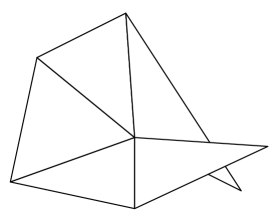
The growth process described above can be characterized by a stochastic grammar. We note however that this grammar will not only generate triangulated polygons, but will also generate objects with overlapping parts as illustrated in Figure 5.

There are two types of symbols in the grammar, corresponding to triangles created during growth ${\cal T}$ and dashed edges that still need to grow ${\cal E}$. Triangles created during growth are elements of ${\cal T}=\{0,1,2\}\times\mathbb{R}^{2}\times\mathbb{R}^{2}\times\mathbb{R}^{2}$. The element $(i,a,b,c)\in{\cal T}$ specifies a triangle of type $i$ with vertices $x_{0}=a$, $x_{1}=b$, $x_{3}=c$ following the labeling in Figure 3. Edges that still need to grow are elements of ${\cal E}=\mathbb{R}^{2}\times\mathbb{R}^{2}$. The element $(a,b)\in{\cal E}$ specifies an internal edge of the triangulated polygon from point $a$ to point $b$, The edges are oriented from $a$ to $b$ so the system can “remember” the direction of growth. Figure 6 illustrates the production rules for the grammar. Note that there are two different rules to grow a triangle of type 1, corresponding to a choice of how the new triangle is glued to the edge that is growing. We simply let both choices have equal probability, $t_{1}/2$.

Figure 5: In principle our growth process can generate objects with overlapping parts.

Figure 6: Production rules for the shape grammar. The grammar generates triangles and oriented edges. The variables $a$, $b$ and $c$ correspond to locations in the plane. The three variables are selected in a production from the start symbol, but only $c$ is selected in a production from an edge. Note that edges are oriented carefully so that growth continues along a particular direction.

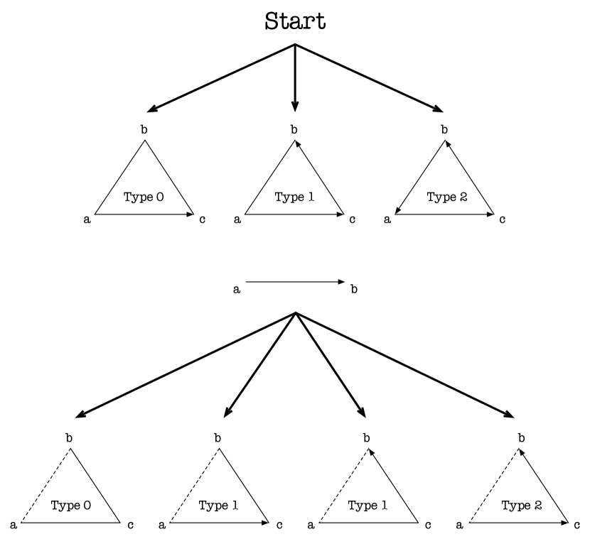
To understand the effect of the parameters $t_{0},t_{1},t_{2}$, consider the dual graph of a triangulated polygon generated by our stochastic process. The growth of the dual graph starts in a root node that has one, two or three children with probability $t_{0}$, $t_{1}$ and $t_{2}$ respectively. Now each child of the root grows according to a Galton-Watson process Habib , where each node has $i$ children with probability $t_{i}$.

An important parameter of a Galton-Watson process is the expected number of children for each node, or Malthusian parameter, that we denote by $m$. In our process, $m=t_{1}+2t_{2}$. When $m<1$ the probability that the growth process eventually terminates is one. From now on we will always assume that $m<1$, which is equivalent to requiring that $t_{2}<t_{0}$ (here we use that $t_{0}+t_{1}+t_{2}=1$).

Let $e$, $b$ and $j$ be random variables corresponding to the number of end, branch and junction triangles in a random shape. Let $n=e+b+j$ be the total number of triangles in a shape. For our Galton-Watson process (corresponding to growth from each child of the root of the dual graph) we can compute the expected number of nodes generated, which we denote by $x$,

$$x=1+(x)t_{1}+(2x)t_{2}\;\Rightarrow\;x=1/(t_{0}-t_{2}).$$

The total number of triangles in a shape is obtained as one node for the root of the dual graph plus the number of nodes in the subtrees rooted at each child of the root. So the expected value of $n$ is,

$$E(n)=1+(x)t_{0}+(2x)t_{1}+(3x)t_{2}.$$

Substituting for $x$ we get,

$$E(n)=\frac{2}{t_{0}-t_{2}}.$$ (1)

Similarly we can compute the expected value of $j$, the number of junction triangles in a shape. This quantity is interesting because it gives a measure of the complexity of the shape. In particular it is a measure of the number of parts (limbs, necks, etc). For the Galton-Watson process, let $y$ be the expected number of nodes with degree 3 (two children),

$$y=(y)t_{1}+(1+2y)t_{2}\;\Rightarrow\;y=t_{2}/(t_{0}-t_{2}).$$

The number of junction triangles in a shape equals the number of such triangles in each subtree of the root plus one if the root itself is a junction triangle,

$$E(j)=(y)t_{0}+(2y)t_{1}+(1+3y)t_{2}.$$

Substituting for $y$ we get,

$$E(j)=\frac{2t_{2}}{t_{0}-t_{2}}.$$ (2)

Equations (1) and (2) provide intuition to the effect of the parameters $t_{0},t_{1},t_{2}$. The equations also show that the parameters are uniquely defined by the expected number of triangles and the expected number of junction triangles in a random shape. We can compute the $t_{i}$ corresponding to any pair $E(n)$ and $E(j)$ such that $E(n)\geq 2$ and $E(n)\geq 2E(j)+2$. These requirements are necessary since the growth process always creates at least two triangles and the number of triangles is always at least twice the number of junction triangles plus two.

$$t_{0} = (2+E(j))/E(n),$$

$$t_{1} = 1-(2E(j)+2)/E(n),$$

$$t_{2} = E(j)/E(n).$$

While the $t_{i}$ control the combinatorial structure of the random shapes we generate, their geometry is highly dependent on the choice of shape for each triangle. The triangle shapes are chosen according to distributions that depend on the triangle type. As an example we can define,

$$s_{i}([X])\propto e^{-k_{i}\operatorname{def}(X_{i},X)^{2}},$$

where $X_{i}$ is an ideal triangle of type $i$ and $\operatorname{def}(X_{i},X)$ is the log-anisotropy of the affine map taking $X_{i}$ to $X$ (see Dryden ; thesis ). The constant $k_{i}$ controls how much the individual traingle shapes are allowed to vary. For the experiments in this chapter we chose both $X_{0}$ and $X_{2}$ to be equilateral triangles and $X_{1}$ to be isosceles, with a smaller side corresponding to the polygon boundary edge. This choice for $X_{1}$ generates shapes that tend to have smooth boundaries. Figure 7 shows what happens when we connect multiple triangles of this type with alternating or similar orientations.

Figure 7: Connecting multiple type 1 triangles in alternating orientations to form an elongated branch, and with the same orientation to form a bend. If the neck triangles tend to be isosceles and thin than the shape boundary tends to be smooth.

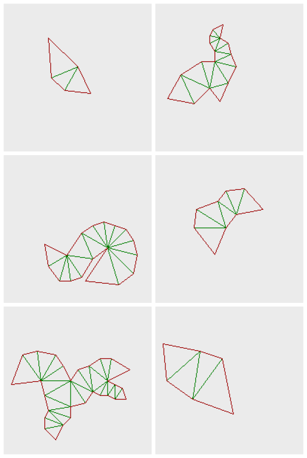
Figure 8 shows some random shapes generated by the random process with $E(n)=20$, $E(j)=1$, and the choice for $s_{i}([X])$ described above. Note how the shapes have natural decompositions into parts, and each part has an elongated structure, with smooth boundaries almost everywhere. These examples illustrate some of the regularties captured by our stochastic shape grammar. In the next section we will show how the grammar can be used for object detection.

Figure 8: Examples of random shapes generated by the stochastic grammar.

3 Sampling Shapes From Images

Now we describe how our model for random shapes can be combined with a likelihood function to yield a posterior distribution $p(T|I)$ over triangulated polygons in an image. We then show how to sample from the posterior using a dynamic programming procedure. The approach is similar to sampling from the posterior distribution of a hidden Markov model using weights computed by the forward-backward algorithm Rabiner . Our experiments in the next Section illustrate how samples from $p(T|I)$ provide hypotheses for the objects in an image.

Recall that each triangle created during growth is an element of ${\cal T}$, specifying a triangle type and the location of its vertices. We assume that the likelihood $p(I|T)$ factors into a product of terms, with one term for each triangle,

$$p(I|T)\propto\prod_{(i,x_{0},x_{1},x_{2})\in T}\pi_{i}(x_{0},x_{1},x_{2},I).$$ (3)

This factorization allows for an efficient inference algorithm to be developed to generate samples from the posterior $p(T|I)\propto p(I|T)p(T)$.

We expect the image to have high gradient at the boundary of objects, with orientation perpendicular to the boundary. In practice we have used a likelyhood function of the form,

$$P(I|T)\propto\exp\left(\lambda\int\|(\nabla I\circ f)(s)\times f^{\prime}(s)\|\;ds\right).$$

Here $f(s)$ is a parametrization of the boundary of $T$ by arclength. The term $\|(\nabla I\circ f)(s)\times f^{\prime}(s)\|$ is the component of the image gradient that is perpendicular to the object boundary at $f(s)$. The integral above can be broken up into a sum of terms, with one term for each boundary edge in the triangulated polygon. This allows us to write the likelihood in the form of equation (3) where $\pi_{i}(x_{0},x_{1},x_{2},I)$ evaluates the contribution to the integral due to the boundary terms (solid edges) of a triangle of type $i$ with vertices $(x_{0},x_{1},x_{2})$.

Let $T_{r}$ denote a triangulated polygon rooted at a triangle $r$. Using Bayes’ law we can write the posterior distribution for rooted shapes given an observed image as,

$$p(T_{r}|I)\propto p(T_{r})p(I|T).$$

There are two approximations we make to sample from this posterior efficiently. We consider only shapes where the depth of the dual graph is bounded by a constant $d$ (the depth of a rooted graph is the maximum distance from a leaf to the root). This should not be a significant problem since shapes with too many triangles have low prior probability anyway. Moreover, the running time of our sampling algorithm is linear in $d$, so we can let this constant be relatively large. We also only consider shapes where the location of each vertex is constrained to lie on a finite grid ${\cal G}$, as opposed to an arbitrary location in the plane. The running time of our algorithm for sampling from $p(T|I)$ is $O(d|{\cal G}|^{3})$.

To sample from the posterior we first pick a root triangle, then pick the triangles connected to the root and so on. The root triangle $r$ should be selected according to its marginal conditional distribution,

$$p(r|I)=\sum_{T_{r}}p(T_{r}|I).$$ (4)

Note that the sum is over all shapes rooted at $r$, and with the depth of the dual graph bounded by $d$. We can compute this marginal distribution in polynomial time because the triangles in a shape are connected together in a tree structure.

Figure 9: A partial shape generated from the edge $(a,b)$.

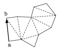
Let $T_{(a,b)}$ denote a partial shape generated from an edge $(a,b)$. Figure 9 shows an example of a partial shape. We denote the probability that the grammar would generate $T_{(a,b)}$ starting from the edge $(a,b)$ by $p(T_{(a,b)})$. The posterior probability of a partial shape $T_{(a,b)}$ given an image $I$ is given by,

$$p(T_{(a,b)}|I)\propto p(T_{(a,b)})\prod_{(i,x_{0},x_{1},x_{2})\in T_{(a,b)}}\pi_{i}(x_{0},x_{1},x_{2},I).$$

We define the following quantities in analogy to the backward weights of a hidden Markov nodel (see Rabiner ),

$$V_{j}(a,b)=\sum_{T_{(a,b)}}p(T_{(a,b)}|I),$$

where the sum is taken over all partial shapes with depth at most $j$. Here we measure depth by imagining the root to be a triangle that would be immediately before the edge $(a,b)$. The quantities $V_{j}(a,b)$ can be computed recursively using a dynamic programming procedure,

$$V_{0}(a,b) = 0,$$

$$V_{j}(a,b) = t_{0}\sum_{c}\,s_{0}([b,c,a])\,\pi_{0}(b,c,a,I)+$$

$$(t_{1}/2)\sum_{c}\,s_{1}([b,c,a])\,\pi_{1}(b,c,a,I)\,V_{j-1}(a,c)+$$

$$(t_{1}/2)\sum_{c}\,s_{1}([c,a,b])\,\pi_{1}(c,a,b,I)\,V_{j-1}(c,b)+$$

$$t_{2}\sum_{c}\,s_{2}([b,c,a])\,\pi_{2}(b,c,a,I)\,V_{j-1}(a,c)\,V_{i-1}(c,b).$$

Now, depending on the type of the root triangle we can rewrite the marginal distribution in equation (4) as,

$$p((0,a,b,c)|I) \propto t_{0}\,s_{0}([a,b,c])\,V_{d}(a,c),$$

$$p((1,a,b,c)|I) \propto t_{1}\,s_{1}([a,b,c])\,V_{d}(a,c)\,V_{d}(c,b),$$

$$p((2,a,b,c)|I) \propto t_{2}\,s_{2}([a,b,c])\,V_{d}(a,c)\,V_{d}(c,b)\,V_{d}(b,a).$$

The equations above provide a way to sample the root triangle from its marginal distribution. The running time for computing all the $V_{j}(a,b)$ and the marginal distribution for the root triangle is $O(d|{\cal G}|^{3})$. Once we compute these quantities we can obtain samples for the root by sampling from a discrete distribution. After choosing $r=(i,x_{0},x_{1},x_{2})$ we need to sample the triangles connected to the root. We then sample the triangles that are at distance two from the root, and so on. When sampling a triangle at distance $j$ from the root, we have an edge $(a,b)$ that is growing. We need to sample a triangle by selecting the location ${\bf c}$ of a new vertex and a triangle type according to

$$p((0,b,{\bf c},a)|I,(a,b)) \propto t_{0}\,s_{0}([b,{\bf c},a]),$$

$$p((1,b,{\bf c},a)|I,(a,b)) \propto (t_{1}/2)\,s_{1}([b,{\bf c},a])\,V_{d-j}(a,{\bf c}),$$

$$p((1,{\bf c},a,b)|I,(a,b)) \propto (t_{1}/2)\,s_{1}([{\bf c},a,b])\,V_{d-j}({\bf c},b),$$

$$p((2,b,{\bf c},a)|I,(a,b)) \propto t_{2}\,s_{2}([b,{\bf c},a])\,V_{d-j}(a,{\bf c})\,V_{d-j}({\bf c},b).$$

We evaluate these probabilities using the precomputed $V_{j}$ quantities and then sample a triangle type and location $c$ from the corresponding discrete distribution. Note that for a triangle at depth $d$ the only choices with non-zero probability will have type zero, as $V_{0}(a,b)=0$.

4 Experimental Results

For the experiments in this section we used a grid ${\cal G}$ of $40\times 40$ locations for the vertices of the shapes. We used the likelihood model defined in the last section, and the same grammar parameters used to generate the random shapes in Figure 8.

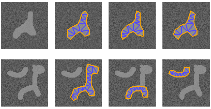
Figure 10 shows some of the samples generated from the posterior distribution $p(T|I)$ for two different synthetic images. The first image has a single object and each sample from $p(T|I)$ gives a slightly different representation for that object. The second image has two objects and the samples from $p(T|I)$ are split between the two objects. Note that we obtain samples that correspond to each object and also to a part of one object that can be naturally interpreted as a single object. Overall the samples in both cases give resonable interpretations of the objects in the images.

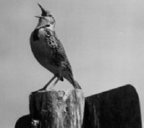
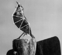
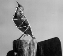
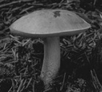
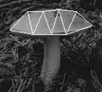
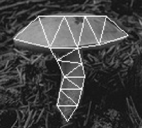
Figures 11 and 12 show samples from the posterior distributon $p(T|I)$ for two natural images. In practice we obtain groups of samples that are only slightly different from each other, and here we show representatives from each group. For the mushroom image, we obtained different samples corresponding to competing interpretations. In one case the whole mushroom is considered as an object, while in another case the stem comes out on its own.

Figure 10: Samples from $p(T|I)$ for two synthetic images $I$. Note how in the second image we get multiple potential objects among the samples.

Figure 11: Sample from $p(T|I)$ for an image with a bird.

Figure 12: Samples from $p(T|I)$ for an image with a mushroom.

References

- [1] Mark De Berg, Otfried Cheong, Marc Van Kreveld, and Mark Overmars. Computational geometry: algorithms and applications. Springer, 2008.
- [2] I.L. Dryden and K.V. Mardia. Statistical Shape Analysis. John Wiley & Sons, 1998.
- [3] P. F. Felzenszwalb. Representation and Detection of Shapes in Images. PhD thesis, MIT, September 2003.
- [4] M. Habib, C. McDiarmid, J. Ramirez-Alfonsin, and B. Reed. Probabilistic Methods for Algorithmic Discrete Mathematics. Springer-Verlag, 1998.
- [5] F. Harary, Palmer E.M., and R.C. Read. On the cell-growth problem for arbitrary polygons. Discrete Mathematics, 11:371–389, 1975.
- [6] D.W. Jacobs. Robust and efficient detection of salient convex groups. IEEE Transactions on Pattern Analysis and Machine Intelligence, 18(1):23–37, 1996.
- [7] I.H. Jermyn and H. Ishikawa. Globally optimal regions and boundaries as minimum ratio weight cycles. IEEE Transactions on Pattern Analysis and Machine Intelligence, 23(10):1075–1088, October 2001.
- [8] M.S. Lee and G. Medioni. Grouping ., -, –¿, 0, into regions, curves, and junctions. Computer Vision and Image Understanding, 76(1):54–69, 1999.
- [9] D. Mumford. Elastica and computer vision. In Algebraic Geometry and Its applications, pages 491–506. Springer-Verlag, 1994.
- [10] M. Nitzberg and D. Mumford. The 2.1-d sketch. In ICCV, pages 138–144, 1990.
- [11] L. R. Rabiner. A tutorial on hidden markov models and selected applications in speech recognition. Proceedings of the IEEE, 77(2), February 1989.
- [12] A. Shashua and S. Ullman. Structural saliency: The detection of globally salient structures using a locally connected network. In ICCV, pages 321–327, 1988.
- [13] S.C. Zhu. Embedding gestalt laws in markov random fields. IEEE Transactions on Pattern Analysis and Machine Intelligence, 21(11):1170–1187, 1999.