The Balancing Act Of Template Bank Construction:
Inspiral Waveform Template Banks For Gravitational-Wave Detectors
And Optimizations At Fixed Computational Cost

Abstract

Gravitational-wave searches for signals from inspiralling compact binaries have relied on matched filtering banks of waveforms (called template banks) to try to extract the signal waveforms from the detector data. These template banks have been constructed using four main considerations, the region of parameter space of interest, the sensitivity of the detector, the matched filtering bandwidth, and the sensitivity one is willing to lose due to the granularity of template placement, the latter of which is governed by the minimal match. In this work we describe how the choice of the lower frequency cutoff, the lower end of the matched filter frequency band, can be optimized for detection. We also show how the minimal match can be optimally chosen in the case of limited computational resources. These techniques are applied to searches for binary neutron star signals that have been previously performed when analyzing Initial LIGO and Virgo data and will be performed analyzing Advanced LIGO and Advanced Virgo data using the expected detector sensitivity. By following the algorithms put forward here, the volume sensitivity of these searches is predicted to improve without increasing the computational cost of performing the search.

I Introduction

For the past decade, large scale interferometric gravitational-wave (GW) detectors have operated, allowing searches for signals from inspiralling compact binaries to be performed Tagoshi et al. (2001); Takahashi et al. (2004); Abbott et al. (2004, 2005a, 2005b, 2006a, 2006b, 2008a, 2008b, 2009a, 2009b); Abadie et al. (2010a, 2011, 2012, b); The LIGO Scientific Collaboration and Hurley (2008); The LIGO Scientific Collaboration et al. (2012); Briggs et al. (2012). These searches have thus far detected no GW signals, however once the detectors are upgraded to their advanced configurations, multiple events are expected to be detected each year The LIGO Scientific Collaboration (2010).

Searches for inspiral signals in detector data depend on matched filtering the data with template waveforms to produce signal-to-noise ratio (SNR) time-series, the maxima of which are used to produce GW “triggers”. Important criteria in constructing banks of template waveforms (i.e., template banks) for these searches are the region of parameter space to be searched, the sensitivity of the detector, the lower and upper frequency cutoffs associated with matched filtering the data, and the maximum fractional loss of SNR (the complement of which is more commonly know as the minimal match) that one is willing to tolerate due to granularity of the template placement. Of these criteria, one is free to tune the lower frequency cutoff and the minimal match due to sensitivity and computational cost considerations.

In Babak et al. (2006), the authors discuss the issue of balancing computational cost versus SNR gain while decreasing the lower frequency cutoff. However, they do not venture so far as to derive the optimal choices. Instead, they choose to set the lower frequency cutoff at a level such that one would lose less than 1% of the SNR by the cutoff being different from 0. In addition, they choose the minimal match of the template bank to be $MM=95\%$; large enough that the metric estimate of the fractional SNR loss is still valid but small enough for computational cost considerations. Recent searches for GW from inspiralling compact binaries have chosen a larger value for the minimal match, $MM=97\%$, so that less than 10% of the signals at the worst mismatch locations of the template bank would be lost.

In this paper, we further investigate the effects of different lower frequency cutoff and minimal match choices. In Sec. III we look at how decreasing the lower frequency cutoff both increases the amount of raw SNR one is able to extract from a signal and increases the trials factor by increasing the number of templates required to search for the waveforms. Sec. IV goes on to describe how to choose the optimal combination of lower frequency cutoff and minimal match for a fixed computational cost. Examples of both these choices are given in Sec. V where the methods are applied to previous and future searches of GW detector data.

II Preliminaries

In searching for signals from inspiralling compact objects in GW data, a commonly used event identification algorithm relies on matched filtering, where the data is “whitened” and filtered with the template waveform being searched for. Specifically, the square SNR is given by

$$\rho^{2}=\frac{(s|h_{c})^{2}+(s|h_{s})^{2}}{\sigma^{2}},$$ (1)

where $s$ is the data from a detector that may contain a GW signal of unknown strength, $h_{c}$ and $h_{s}$ are the target waveforms associated with the same source and differ in phase by $\pi/4$, $\sigma^{2}:=(h_{c}|h_{c})$ is the sensitivity of our detector to a waveform at a reference distance, typically chosen to be 1 Mpc, and the inner product $(x|y)$ is defined as

$$(x|y):=4\Re\int_{f_{\rm low}}^{f_{\rm high}}\frac{\tilde{x}\tilde{y}^{*}}{S_{n}(f)}df.$$ (2)

Here $\tilde{x}$ is the Fourier transform of $x$, $()^{*}$ denotes the complex conjugate operator, and $S_{n}(f)$ is the one-sided power spectral density (PSD) of the detector’s noise.

As can be seen from (2), the SNR recovered when there is a signal present in the data will depend on the limits of the integration. The upper frequency cutoff $f_{\rm high}$ is set by the lower of either the Nyquist frequency of the data or the maximum frequency of the template waveform. In contrast, the lower frequency cutoff $f_{\rm low}$ is a parameter that can be tuned in optimizing the search algorithm.

To search a region of parameter space, many template waveforms from points spread throughout the region need to be matched filtered. The locations of these points are chosen by constructing a metric on the parameter space $g_{ij}$ Owen (1996); Owen and Sathyaprakash (1999); Brown et al. (2012); Keppel et al. (2012). This metric describes the distance between points based on the fractional loss of SNR associated with matched filtering a signal waveform from one point in parameter space with a template waveform from another point. To second order in the parameter differences $\Delta\lambda^{i}$, the fractional loss of SNR, or mismatch $m$, is given by

$$m=\frac{1}{2}g_{ij}\Delta\lambda^{i}\Delta\lambda^{j},$$ (3)

where the metric is given by projecting out dimensions of the parameter space from normalized Fisher matrix,

$$g_{\mu\nu}:=\frac{(\partial_{\mu}h|\partial_{\nu}h)}{(h|h)},$$ (4)

that are associated with extrinsic parameters, which can be maximized either analytically or efficiently. Here $\partial_{\mu}$ is the partial derivative with respect to parameter $\lambda^{\mu}$. The density of templates is then governed by the maximum amount of mismatch one is willing to tolerate, or the complement of this, referred to as the minimal match $MM=1-m$.

III Signal Power versus Trials Factor: Optimizing The Lower Frequency Cutoff For Maximum Sensitivity

The goal of designing a search is to maximize the volume at which we are sensitive to signals for a fixed false alarm probability (FAP). The first parameter we tune with this in mind is the lower frequency cutoff. We start with the distance out to which we can see an inspiral signal with a fixed SNR $\rho$,

$$D=\frac{\sigma}{\rho}.$$ (5)

Changing the lower frequency cutoff changes the power of the signal that we could possibly recover. If one were to recover a signal with the same SNR, the distance to which one could see a signal would vary when the lower frequency cutoff was changed from $f_{\rm ref}$ to $f_{\rm low}$,

$$\frac{D(f_{\rm low})}{D(f_{\rm ref})}=\frac{\sigma(f_{\rm low})}{\sigma(f_{\rm ref})}.$$ (6)

Let us now look at how the observable distance of a signal is affected when the signal is recovered with a mismatched template. The observed SNR $\rho$ will be reduced from the SNR obtained by a template that matches the signal $\rho_{\rm ref}$ by

$$\rho=\rho_{\rm ref}(1-m),$$ (7)

where $m$ is the mismatch between the template that recovers the signal and the actual signal. Eq. 5 implies that the distance to which such a signal will be observable is reduced by the same factor

$$\frac{D(f_{\rm ref},m)}{D(f_{\rm ref},0)}=(1-m).$$ (8)

So far we have focused on the obserable distance of a signal at fixed SNR. However it is actually the obserable distance of a signal at fixed FAP that we are interested in. The FAP associated with a single observation of SNR $\rho$ is given by

$$\mathrm{FAP}\propto\exp[-\rho^{2}].$$ (9)

The recovered FAP is subject to a trials factor related to the number of independent trials $N$ we use in looking for a signal,

$$\mathrm{FAP}^{\prime}=1-(1-\mathrm{FAP})^{N}\approx N\mathrm{FAP}.$$ (10)

We can translate a single observation of $\rho_{\rm observed}$ among $N$ independent trials to a reference SNR $\rho_{\rm ref}$ among a different number of trials $N_{\rm ref}$ at the same FAP by combining (9) and (10).

$$\rho_{\rm observed}^{2}=\rho_{\rm ref}^{2}+\ln\frac{N}{N_{\rm ref}}.$$ (11)

When searching a non-zero measure region of parameter space, additional trials are accrued proportional to the volume of the parameter space. The volume of parameter space is in turn given by the number of templates needed to cover the parameter space $M_{\rm templates}$ Prix (2007),

$$N_{\rm trials}\propto\int\sqrt{\left|g\right|}d\lambda^{d}=\frac{M_{\rm templates}m^{d/2}}{\theta}$$ (12)

where $\sqrt{\left|g\right|}$ is the square root of the determinant of the metric on the space, $\theta$ is a geometrical quantity associated with how the template bank tiles the parameter space, $m=1-MM$ is maximum mismatch allowed in the template bank covering the parameter space, and $d$ is the dimensionality of the parameter space being tiled (i.e., two for templates associated with waveforms from non-spinning objects that are laid out in the two dimensional mass space).

Since the metric (4) is defined in terms of the inner products from (2), the full metric itself is a function of the lower frequency cutoff, which in turn implies that the metric density of the mass subspace is also a function of $f_{\rm low}$,

$$\sqrt{|g|}=\sqrt{|g(f_{\rm low})|}.$$ (13)

The total volume we can observe is proportional to the cube of the distance, thus the ratio of the volume we can observe for a mismatched signal at a given value of $f_{\rm low}$ to the volume we could observe a matched signal with a reference lower frequency cutoff $f_{\rm ref}$ is found by combining (6), (8), (11), (12), and (13),

$$\frac{V(f_{\rm low},m)}{V(f_{\rm ref},0)}=\frac{\sigma^{3}(f_{\rm low})}{\sigma^{3}(f_{\rm ref})}\\ \times\frac{(1-m)^{3}}{\left(1+\frac{1}{\rho^{2}(f_{\rm ref})}\ln\left[\frac{\int\sqrt{\left|g(f_{\rm low})\right|}d\lambda^{d}}{\int\sqrt{\left|g(f_{\rm ref})\right|}d\lambda^{d}}\right]\right)^{3/2}}.$$ (14)

We call this the relative volume. For two-dimensional template banks, a hexagonal covering of templates following the $A_{2}^{*}$ lattice will result in a distribution of mismatches that is essentially flat between 0 and the maximum mismatch Prix (2007). Using this fact, the average relative volume is found to be

$$\frac{\left\langle V(f_{\rm low},m)\right\rangle}{\left\langle V(f_{\rm ref},0)\right\rangle}=\frac{\sigma^{3}(f_{\rm low})}{\sigma^{3}(f_{\rm ref})}\\ \times\frac{\left\langle\left(1-m\right)^{3}\right\rangle}{\left(1+\frac{1}{\rho^{2}(f_{\rm ref})}\ln\left[\frac{\int\sqrt{\left|g(f_{\rm low})\right|}d\lambda^{d}}{\int\sqrt{\left|g(f_{\rm ref})\right|}d\lambda^{d}}\right]\right)^{3/2}},$$ (15)

where the average of the mismatch term in the numerator is given by

$$\left\langle\left(1-m\right)^{3}\right\rangle=1-\frac{3}{2}m+m^{2}-\frac{1}{4}m^{3}.$$ (16)

The average relative volume can be maximized with the proper choice of $f_{\rm low}$ for a fixed value of the template bank maximum mismatch.

IV Wider or Denser?: Maximizing Sensitivity At Fixed Computational Cost

In the face of limited computational resources, we must consider not only how to maximize the sensitivity of a search through the choice of the lower frequency cutoff, but we must also ensure that our choices of the lower frequency cutoff and the minimal match satisfy the constraint on the total computational cost $C_{\rm total}$. This constraint can be viewed as a combination of two effects: the computational cost of filtering the data with a single template waveform $C_{\rm filter}$ multiplied by the computational cost associated with $N_{\rm templates}$ such filters

$$C_{\rm total}(f_{\rm low})= N_{\rm templates}(f_{\rm low})C_{\rm filter}(f_{\rm low})$$

$$= C_{\rm filter}(f_{\rm low})\theta m^{-d/2}\int\sqrt{\left|g(f_{\rm low})\right|}d\lambda^{d}.$$ (17)

Using this constraint, we seek to maximize the constrained average relative volume

$$\frac{\left\langle V(f_{\rm low})\right\rangle}{\left\langle V(f_{\rm ref})\right\rangle}= \frac{\sigma^{3}(f_{\rm low})}{\sigma^{3}(f_{\rm ref})}\frac{\left\langle\left(1-m(f_{\rm low})\right)^{3}\right\rangle}{\left\langle\left(1-m(f_{\rm ref})\right)^{3}\right\rangle}$$

$$\times\frac{1}{\left(1+\frac{1}{\rho^{2}(f_{\rm ref})}\ln\left[\frac{\int\sqrt{\left|g(f_{\rm low})\right|}d\lambda^{d}}{\int\sqrt{\left|g(f_{\rm ref})\right|}d\lambda^{d}}\right]\right)^{3/2}},$$ (18)

with the proper choice of $f_{\rm low}$ and $m(f_{\rm low})$.

Assuming one is able to computationally preform the search for a given combination of lower frequency cutoff $f_{\rm ref}$ and maximum mismatch $m(f_{\rm ref})$, the maximum mismatch at any other choice of lower frequency cutoff $f_{\rm low}$ satisfying the constraint on the computational cost can be solved for easily,

$$m(f_{\rm low})=m(f_{\rm ref})\left(\frac{C_{\rm filter}(f_{\rm low})\int\sqrt{\left|g(f_{\rm low})\right|}d\lambda^{d}}{C_{\rm filter}(f_{\rm ref})\int\sqrt{\left|g(f_{\rm ref})\right|}d\lambda^{d}}\right)^{2/d}$$ (19)

The computational cost of filtering data with a single template will depend intrinsically on the implementation of a search. As a first example, it could be independent of the choice of $f_{\rm low}$, as is the case in the FINDCHIRP algorithm Allen et al. (2005) where data is processed with fast Fourier transforms using fixed length chunks.

In a different algorithm where data is analyzed in the time domain using finite impulse response (FIR) filters, the computational cost would be set by the number of taps in the FIR filter. This is proportional to the length of the waveform $T$, given to Newtonian order by

$$T(f_{\rm low})=\frac{5}{256\mathcal{M}^{5/3}}\left[(4\pi f_{\rm low})^{-8/3}-(4\pi f_{\rm high})^{-8/3}\right],$$ (20)

where $\mathcal{M}=(m_{1}m_{2})^{3/5}(m_{1}+m_{2})^{1/5}$ is the chirp mass of the binary system.

Alternatively, if one were able to change the sampling rate associated with the template filter continuously, one could reduce the computational cost by filtering the data with a changing local sampling rate such that the frequency of the signal at any time was always equal to the local Nyquist frequency of the filter. In this approach, the computational cost would be proportional to the number of cycles in the signal waveform,

$$N_{\rm cycles}(f_{\rm low})=\frac{1}{64\pi^{8/3}\mathcal{M}^{5/3}}\left(f_{\rm low}^{-5/3}-f_{\rm high}^{-5/3}\right).$$ (21)

Finally, as an application of this method to a pipeline proposed to search for binary neutron star (BNS) signals with low latency in the Advanced LIGO (aLIGO) sensitive band, we consider the computational cost of the LLOID algorithm Cannon et al. (2012). The LLOID algorithm partitions the waveforms into $S$ time-slices and filters the waveform portions of slice $s$ at a power of two sampling rate $f^{s}$ such that the Nyquist frequency of the slice is just greater than the largest frequency of any of the portions of the waveform in that slice. In addition, for each slice, the LLOID algorithm decomposes the $N_{\rm templates}$ template waveform portions into $L_{\rm bases}^{s}$ basis vectors using singular value decomposition (SVD) Cannon et al. (2010). These basis vectors are used as FIR filters of $N^{s}_{\rm taps}$ taps for slice $s$. The computational cost of filtering a bank of waveforms with this algorithm is dominated by the filtering costs of the basis vectors and the reconstruction costs of turning the basis filter outputs into outputs of template filters,

$$N_{\rm FLOPS}=2\sum_{s=0}^{S-1}f^{s}L^{s}_{\rm bases}(N_{\rm taps}^{s}+N_{\rm templates}).$$ (22)

Let us look at how the different pieces of LLOID’s computational cost will change with varying $f_{\rm low}$. For a particular slice, as $f_{\rm low}$ is reduced, the template waveforms that go into the SVD matrix will more densely cover the region of parameter space, resulting in a larger number of waveforms that will need to be reconstructed (i.e., $N_{\rm templates}$ will increase). However, the number of bases $N^{s}_{\rm bases}$ needed reconstruct the template waveforms to a specific accuracy is invariant for the minimal matches we are interested in Cannon et al. (2011). Finally, the number of slices kept will depend on $f_{\rm low}$ as each slice covers a different frequency range of the waveforms. Thus, the total computational cost of the LLOID algorithm can be written as

$$N_{\rm FLOPS}=A(f_{\rm low})N_{\rm templates}+B(f_{\rm low}),$$ (23)

where $A(f_{\rm low})$ and $B^{s}(f_{\rm low})$ are defined appropriately with respect to (22). For this algorithm, (19) takes a different form,

$$m(f_{\rm low})=m(f_{\rm ref})\left(\frac{A(f_{\rm low})N_{\rm ref}\frac{\int\sqrt{\left|g(f_{\rm low})\right|}d\lambda^{d}}{\int\sqrt{\left|g(f_{\rm ref})\right|}d\lambda^{d}}}{A(f_{\rm ref})N_{\rm ref}+B(f_{\rm ref})-B(f_{\rm low})}\right)^{2/d},$$ (24)

where $N_{\rm ref}:=N_{\rm templates}(f_{\rm low})$.

V Examples

(a) H1 PSDs

(b) V1 PSDs

(c) Harmonic Sum PSDs

Figure 1: LABEL:sub@fig:H1psds shows different PSDs associated with different eras of the H1 LIGO detector. LABEL:sub@fig:V1psds shows different PSDs associated with different eras of the Virgo detector. LABEL:sub@fig:harmonicpsds shows different PSDs associated with detector networks from different eras. The H1H2L1V1 network PSD associated with the S5/VSR1 era is given by the harmonic sum of individual detectors’ PSDs. For the S6/VSR2-3 and aLIGO/AdV eras, an H1L1V1 network is used.

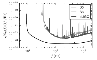
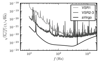
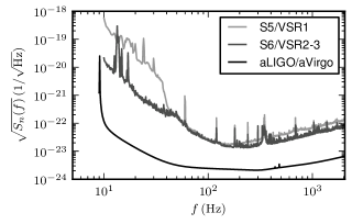
In this section we apply the methods from Secs. III and IV to the (expected) sensitivities of several past and future detectors. In particular, we investigate the LIGO and Virgo PSDs from S5/VSR1 Abadie et al. (2010c), S6/VSR2-3 LIGO:2012aa (1093632); Accadia et al. (2011), and the expected advanced detector PSDs for aLIGO The LIGO Scientific Collaboration (2009) and AdV The Virgo Scientific Collaboration (2010). We also consider joint detector analyses where the individual detectors PSDs are combined by taking the harmonic sum, which yields the same combined SNR as either the coherent network SNR or the sum-of-squares SNR associated with a coincident search Harry and Fairhurst (2011); Keppel (2012). These PSDs can be seen in Fig. 1. The parameter space we focus on for these comparisons is that associated with searches for BNS signals from non-spinning objects. Using the stationary phase approximation, we expand the template waveforms to Newtonian order in the amplitude and 3.5  post-Newtonian (PN) order in the phase. The metric for these waveforms is given in Keppel et al. (2012). With this focus, we approximate the ratio of the integrated metric density by a point estimate such that the mass of each object is 1.4 $M_{\odot}$,

$$\frac{\int\sqrt{\left|g(f_{\rm low})\right|}d\lambda^{d}}{\int\sqrt{\left|g(f_{\rm ref})\right|}d\lambda^{d}}\approx\sqrt{\frac{\left|g_{\rm BNS}(f_{\rm low})\right|}{\left|g_{\rm BNS}(f_{\rm ref})\right|}}.$$ (25)

It should also be noted that, in this approximation, we assume that the effects from the bulk of parameter space dominate over effects from the boundaries. For parameter spaces where the effects of the boundaries are non-negligible, more care will be needed in computing the ratio of the integrated metric densities and how they relate to the trials factor and computational cost.

V.1 Choice of $f_{\rm low}$

Era	Detector	$f^{\textrm{standard}}_{\rm low}$	$f^{\textrm{optimal}}_{\rm low}$	Volume Gain
S5	H1	40Hz	37.3Hz	$6.4\times 10^{-5}$
VSR1	V1	60Hz	38.1Hz	$1.9\times 10^{-2}$
S5/VSR1	H1H2L1V1	40Hz	37.8Hz	$4.9\times 10^{-5}$
S6	H1	40Hz	43.7Hz	$2.5\times 10^{-5}$
VSR2-3	V1	50Hz	16.8Hz	$1.5\times 10^{-1}$
S6/VSR2-3	H1L1V1	40Hz	34.0Hz	$7.0\times 10^{-4}$
aLIGO	H1	10Hz	9.6Hz	$1.3\times 10^{-5}$
AdV	V1	10Hz	17.6Hz	$1.7\times 10^{-3}$
aLIGO/AdV	H1L1V1	10Hz	10.1Hz	$8.6\times 10^{-7}$

Table 1: We show the increase in the average relative volume (15) that can be achieved by switching from the standard lower frequency cutoff to the optimal lower frequency cutoff. The minimal match in either case is set to be 3%. The volume increase compared to the standard choice is very small, except for the V1 VSR1 PSD, where a higher than normal lower frequency cutoff was employed.

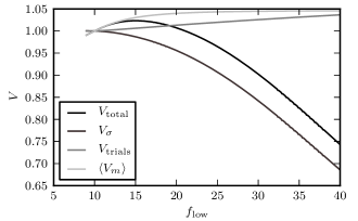
First we optimize the choice of the lower frequency cutoff of an inspiral search for different detectors without regard to the computational cost. Table 1 summarizes the results for all of the detector combinations mentioned, compared to the “standard” choice of the lower frequency cutoff. For the most part, this is a very small effect, as can be anticipated through the logarithmic dependence of the effect of the trials factor in (15). The largest differences between the standard choice and the optimal choice occur for the Virgo detector during VSR1, which increases the sensitivity of the search by $15\%$. This seems to be attributed to a rapid decrease in the recoverable SNR that is seen between about 55Hz and 60Hz.

Era	Detector	$f^{\textrm{minimum}}_{\rm low}$	$f^{\textrm{optimal}}_{\rm low}$	Volume Gain
S5	H1	30Hz	37.3Hz	$2.0\times 10^{-6}$
VSR1	V1	10Hz	38.1Hz	$3.5\times 10^{-5}$
S5/VSR1	H1H2L1V1	10Hz	37.8Hz	$1.7\times 10^{-4}$
S6	H1	40Hz	43.7Hz	$2.5\times 10^{-5}$
VSR2-3	V1	10Hz	16.8Hz	$1.1\times 10^{-3}$
S6/VSR2-3	H1L1V1	10Hz	34.2Hz	$5.5\times 10^{-3}$
aLIGO	H1	9Hz	9.6Hz	$2.5\times 10^{-6}$
AdV	V1	10Hz	17.6Hz	$1.7\times 10^{-3}$
aLIGO/AdV	H1L1V1	9Hz	10.1Hz	$2.2\times 10^{-5}$

Table 2: Similar to Table 1, we show the increase in the average relative volume (15) that can be achieved by switching to the optimal lower frequency cutoff. However, here the reference lower frequency cutoff is set to the minimum frequency at which a detector’s PSD is reported.

(a) H1 S5 PSD

(b) V1 VSR1 PSD

(c) H1H2L1V1 S5/VSR1 Harmonic Sum PSD

Figure 2: LABEL:sub@fig:H1S5mm shows the average relative volume $V_{\rm total}$ as a function of lower frequency cutoff for the H1 LIGO detector during the S5 era. LABEL:sub@fig:V1VSR1mm and LABEL:sub@fig:H1H2L1V1S5VSR1mm show the same for the Virgo detector and H1H2L1V1 detector network for the VSR1 and S5/VSR1 eras, respectively. Each panel also contains traces for the contributions to the average relative volume from the recoverable SNR $V_{\sigma}$ and the trials factor $V_{\rm trials}$.

(a) H1 S6 PSD

(b) V1 VSR2-3 PSD

(c) H1L1V1 S6/VSR2-3 Harmonic Sum PSD

Figure 3: LABEL:sub@fig:H1S6mm shows the average relative volume as a function of lower frequency cutoff for the H1 LIGO detector during the S6 era. LABEL:sub@fig:V1VSR23mm and LABEL:sub@fig:H1L1V1S6VSR23mm show the same for the Virgo detector and H1L1V1 detector network for the VSR2-3 and S6/VSR2-3 eras, respectively. Each panel also contains traces for the contributions to the average relative volume from the recoverable SNR $V_{\sigma}$ and the trials factor $V_{\rm trials}$.

(a) H1 aLIGO PSD

(b) V1 AdV PSD

(c) H1L1V1 aLIGO/AdV Harmonic Sum PSD

Figure 4: LABEL:sub@fig:H1aLIGOmm shows the average relative volume as a function of lower frequency cutoff for the proposed H1 LIGO detector during the aLIGO era. LABEL:sub@fig:V1aVirgomm and LABEL:sub@fig:H1L1V2aLIGOaVirgomm show the same for the proposed Virgo detector and H1L1V1 detector network for the AdV and aLIGO/AdV eras, respectively. Each panel also contains traces for the contributions to the average relative volume from the recoverable SNR $V_{\sigma}$ and the trials factor $V_{\rm trials}$.

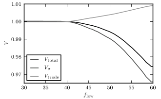
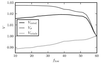
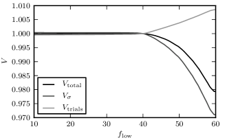
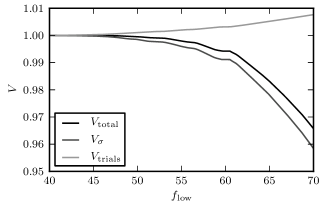
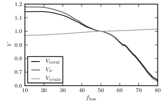
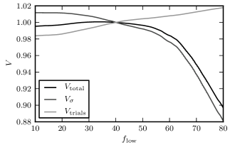
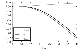
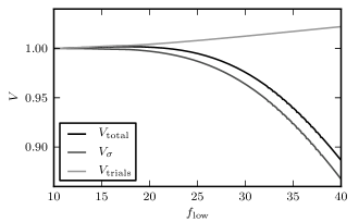
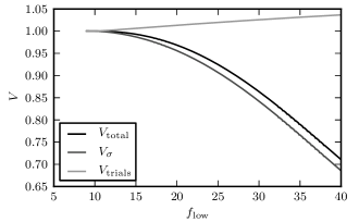
Table 2 makes a similar comparison, although here the standard lower frequency cutoff choice is replaced by the minimum reported frequency associated with a particular PSD. It is particularly interesting to see the trials factor effect associated with the Virgo detector during VSR1. In that case, the difference between the minimum choice of 10Hz and the optimal choice of 38.1Hz is a few parts in $10^{5}$. What is interesting about this comparison is the large difference in the lower frequency cutoff choices. As Virgo detector’s PSD from VSR1 had a very shallow slope at the low frequency end, it provides a good example of how the effect of the trials factor can grow more quickly than the SNR gain as the lower frequency cutoff is lowered. More detailed sensitivity comparisons can be found in Figs. 2-4, which separately show the effect of varying lower frequency cutoff on the recovered SNR and on the trials factor effect as a function of the lower frequency cutoff. The example described above associated with the Virgo VSR1 PSD can be seen in Fig. 2b.

V.2 Fixed Computational Cost

Detector	Era	Cost	$f^{\textrm{standard}}_{\rm low}$, $m^{\textrm{standard}}_{\rm max}$	$f^{\textrm{optimal}}_{\rm low}$, $m^{\textrm{optimal}}_{\rm max}$	Volume Gain
S5	H1	Fixed	40Hz, 3%	49.1Hz, 2.4%	$4.5\times 10^{-3}$
VSR1	V1	Fixed	60Hz, 3%	50.1Hz, 2.8%	$6.2\times 10^{-3}$
S5/VSR1	H1H2L1V1	Fixed	40Hz, 3%	50.2Hz, 2.3%	$5.3\times 10^{-3}$
S6	H1	Fixed	40Hz, 3%	55.7Hz, 2.6%	$3.5\times 10^{-3}$
VSR2-3	V1	Fixed	50Hz, 3%	37.8, 6.2%	$1.8\times 10^{-2}$
S6/VSR2-3	H1L1V1	Fixed	40Hz, 3%	51.2Hz, 2.2%	$7.9\times 10^{-3}$
aLIGO	H1	Cycles	10Hz, 3%	14.4Hz, 1.1%	$2.1\times 10^{-2}$
AdV	V1	Cycles	10Hz, 3%	22.0Hz, 0.56%	$3.7\times 10^{-2}$
aLIGO/AdV	H1L1V1	Cycles	10Hz, 3%	15.0Hz, 1.0%	$2.3\times 10^{-2}$
aLIGO/AdV	H1L1V1	LLOID	9.7Hz, 3%	14.2Hz, 0.84%	$2.8\times 10^{-2}$

Table 3: We show the gain in the constrained average relative volume (IV) that can be obtained by changing from the standard choice of lower frequency cutoff and maximum mismatch to the optimal choice. The computational cost for each of these calculations is set using the algorithm listed under “Cost”. Most of these searches are optimized by increasing the lower frequency cutoff and decreasing the maximum mismatch (i.e., increasing the density) of the template bank.

Era	Detector	Cost	$f^{\textrm{previous}}_{\rm low}$, $m^{\textrm{previous}}_{\rm max}$	$f^{\textrm{optimal}}_{\rm low}$, $m^{\textrm{optimal}}_{\rm max}$	Volume Gain
S5	H1	Fixed	57.8Hz, 5%	58.4Hz, 4.9%	$5.3\times 10^{-5}$
VSR1	V1	Fixed	60.0Hz, 5%	50.1Hz, 5.4%	$6.8\times 10^{-4}$
S5/VSR1	H1H2L1V1	Fixed	60.0Hz, 5%	59.7Hz, 5.0%	$3.2\times 10^{-7}$
S6	H1	Fixed	67.1Hz, 5%	63.2Hz, 5.7%	$2.0\times 10^{-3}$
VSR2-3	V1	Fixed	44.7Hz, 5%	43.4Hz, 5.2%	$3.0\times 10^{-4}$
S6/VSR2-3	H1L1V1	Fixed	62.8Hz, 5%	60.3Hz, 5.3%	$6.7\times 10^{-4}$
aLIGO	H1	Cycles	17.0Hz, 5%	19.5Hz, 3.1%	$9.7\times 10^{-3}$
AdV	V1	Cycles	28.8Hz, 5%	31.3Hz, 3.7%	$5.1\times 10^{-3}$
aLIGO/AdV	H1L1V1	Cycles	18.0Hz, 5%	20.8Hz, 3.1%	$1.1\times 10^{-2}$

Table 4: We show the gain in the constrained average relative volume (IV) that can be obtained by changing from the choice of lower frequency cutoff and maximum mismatch proposed in Babak et al. (2006) to the optimal choice. Again, the computational cost for each of these calculations is set using the algorithm listed under “Cost”. The choices of Babak et al. (2006) are close to optimal, although the advanced detector network search can be improved by of order one percent when switching to the optimal choices.

We now consider the task of choosing optimal values for both the lower frequency cutoff and the minimal match of the template bank subject to the constraint of fixed computational cost. Table 3 shows a comparison between the standard values and the optimal values chosen using the algorithm proposed in this paper. In addition to the detector/era associated with a particular PSD and the standard and optimal choices for the minimal match and lower frequency cutoff, this table also lists the computational cost algorithm that is appropriate for a given search.

We see that including the constraint on the computational cost produces a larger effect than optimizing the lower frequency cutoff alone without the constraint. It is interesting to note that for the majority of the cases investigated, the optimal choice involves reducing the computational cost through raising the lower frequency cutoff and then reinvesting the computational savings into increasing the density of the template bank.

(a) H1 S5 PSD

(b) V1 VSR1 PSD

(c) H1H2L1V1 S5/VSR1 Harmonic Sum PSD

Figure 5: LABEL:sub@fig:H1S5cost shows the constrained average relative volume as a function of lower frequency cutoff for the H1 LIGO detector during the S5 era. LABEL:sub@fig:V1VSR1cost and LABEL:sub@fig:H1H2L1V1S5VSR1cost show the same for the Virgo detector and H1H2L1V1 detector network for the VSR1 and S5/VSR1 eras, respectively. The computational cost of the searches associated with these eras is given by the fixed cost algorithm. Each panel also contains traces for the contributions to the constrained average relative volume from the recoverable SNR $V_{\sigma}$, the trials factor $V_{\rm trials}$, and the average template bank mismatch $\langle V_{m}\rangle$.

(a) H1 S6 PSD

(b) V1 VSR2-3 PSD

(c) H1L1V1 S6/VSR2-3 Harmonic Sum PSD

Figure 6: LABEL:sub@fig:H1S6cost shows the constrained average relative volume as a function of lower frequency cutoff for the H1 LIGO detector during the S6 era. LABEL:sub@fig:V1VSR23cost and LABEL:sub@fig:H1L1V1S6VSR23cost show the same for the Virgo detector and H1L1V1 detector network for the VSR2-3 and S6/VSR2-3 eras, respectively. The computational cost of the searches associated with these eras is given by the fixed cost algorithm. Each panel also contains traces for the contributions to the constrained average relative volume from the recoverable SNR $V_{\sigma}$, the trials factor $V_{\rm trials}$, and the average template bank mismatch $\langle V_{m}\rangle$.

(a) H1 aLIGO PSD

(b) V1 AdV PSD

(c) H1L1V1 aLIGO/AdV Harmonic Sum PSD

Figure 7: LABEL:sub@fig:H1aLIGOcost shows the constrained average relative volume as a function of lower frequency cutoff for the proposed H1 LIGO detector during the aLIGO era. LABEL:sub@fig:V1aVirgocost and LABEL:sub@fig:H1L1V2aLIGOaVirgocost show the same for the proposed Virgo detector and H1L1V1 detector network for the AdV and aLIGO/AdV eras, respectively. The computational cost of the searches associated with these eras is given by the cycles cost algorithm, (21). Each panel also contains traces for the contributions to the constrained relative average volume from the recoverable SNR $V_{\sigma}$, the trials factor $V_{\rm trials}$, and the average template bank mismatch $\langle V_{m}\rangle$.

Figure 8: We show the constrained average relative volume as a function of low frequency cutoff for the proposed H1L1V1 detector network during the aLIGO/AdV era. The computational cost of this search is given by the LLOID algorithm. The contributions to the constrained average relative volume from the recoverable SNR $V_{\sigma}$, the trials factor $V_{\rm trials}$, and the average template bank mismatch $\langle V_{m}\rangle$ are also shown. It is interesting to see that the optimal choices for this search are similar to that of a search where the computational cost is given by the number of cycles in the template waveform.

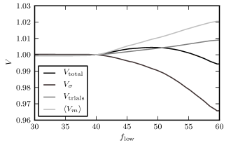
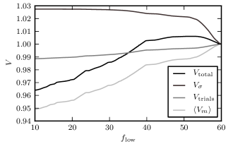
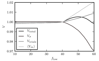
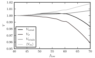
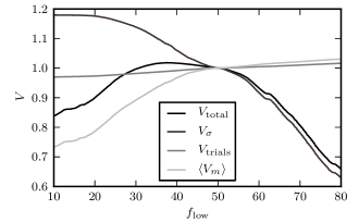
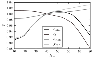
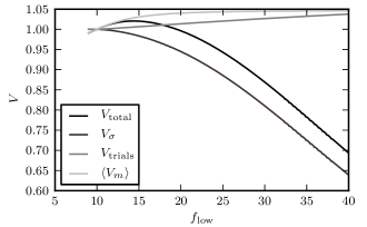
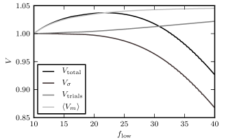
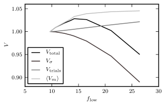
As before, we also show a more detailed comparison of the constrained optimization of the lower frequency cutoff and minimal match as a function of the lower frequency cutoff. This can be found in Figs. 5-8. In this situation, the largest increase in sensitivity is a few percent, coming from the proposed AdV detector’s PSD. Figure 7b shows that the majority of the effect here is coming from decreasing the maximum mismatch (i.e., increasing the minimal match) of the template bank from 3% maximum mismatch to 0.56% maximum mismatch. In this situation, the drive toward larger lower frequency cutoffs seems to come from the reduction in the computational cost per template associated with the total number of cycles contained in the waveform, as opposed to reducing the trials factor effect.

Finally, we also compare the previous choice of lower frequency cutoff and minimal match suggested in Babak et al. (2006) (i.e., $m_{\rm max}=5\%$ and lower frequency cutoff such that fractional SNR loss is 1%) to the optimal choice at the same computational cost. This comparison can be found in Table 4. This choice is closer to the optimal choice, although the optimal choice still provides sensitivity gains as large as one percent for the aLIGO/AdV detector network.

VI Conclusion

We have presented an analysis of the two tunable variables that affect searches for inspiral signals in GW data. We find that with the minimal match of the template bank held fixed, there is an optimal choice for the lower frequency cutoff below which reducing this parameter reduces the sensitivity of a search that employs a maximum likelihood ratio estimate of the SNR. This could be seen as the following inverse result. Even though decreasing the lower frequency cutoff does not gain significant amounts of SNR, it still provides discriminating power in determining the parameters, thus increasing the trials factor associated with a fixed region of parameter space.

In addition, through careful balancing of the computational cost associated with the lower frequency cutoff and the minimal match of the template bank, we show that improved performance can be achieved at fixed computational cost. This is the first work that has laid out a procedure for determining the optimal choice of these parameters for searches for BNS GW signals from non-spinning objects. As searches for inspiral GW signals from other systems can involve additional waveform parameters, and thus larger computational cost, it will be important to apply this method to other parameter spaces (e.g., the parameter space of waveforms from binary systems that including effects from the objects’ spins) in order to maximize the sensitivity of those searches.