FERMILAB-PUB-13-059-E

The D0 Collaboration¹¹1with visitors from ^aAugustana College, Sioux Falls, SD, USA, ^bThe University of Liverpool, Liverpool, UK, ^cUPIITA-IPN, Mexico City, Mexico, ^dDESY, Hamburg, Germany, ^eSLAC, Menlo Park, CA, USA, ^fUniversity College London, London, UK, ^gCentro de Investigacion en Computacion - IPN, Mexico City, Mexico, ^hECFM, Universidad Autonoma de Sinaloa, Culiacán, Mexico, ⁱUniversidade Estadual Paulista, São Paulo, Brazil, ^jKarlsruher Institut für Technologie (KIT) - Steinbuch Centre for Computing (SCC) and ^kOffice of Science, U.S. Department of Energy, Washington, D.C. 20585, USA.

Combined search for the Higgs boson with the D0 experiment

V.M. Abazov Joint Institute for Nuclear Research, Dubna, Russia B. Abbott University of Oklahoma, Norman, Oklahoma 73019, USA B.S. Acharya Tata Institute of Fundamental Research, Mumbai, India M. Adams University of Illinois at Chicago, Chicago, Illinois 60607, USA T. Adams Florida State University, Tallahassee, Florida 32306, USA G.D. Alexeev Joint Institute for Nuclear Research, Dubna, Russia G. Alkhazov Petersburg Nuclear Physics Institute, St. Petersburg, Russia A. Alton^a University of Michigan, Ann Arbor, Michigan 48109, USA A. Askew Florida State University, Tallahassee, Florida 32306, USA S. Atkins Louisiana Tech University, Ruston, Louisiana 71272, USA K. Augsten Czech Technical University in Prague, Prague, Czech Republic C. Avila Universidad de los Andes, Bogotá, Colombia F. Badaud LPC, Université Blaise Pascal, CNRS/IN2P3, Clermont, France L. Bagby Fermi National Accelerator Laboratory, Batavia, Illinois 60510, USA B. Baldin Fermi National Accelerator Laboratory, Batavia, Illinois 60510, USA D.V. Bandurin Florida State University, Tallahassee, Florida 32306, USA S. Banerjee Tata Institute of Fundamental Research, Mumbai, India E. Barberis Northeastern University, Boston, Massachusetts 02115, USA P. Baringer University of Kansas, Lawrence, Kansas 66045, USA J.F. Bartlett Fermi National Accelerator Laboratory, Batavia, Illinois 60510, USA U. Bassler CEA, Irfu, SPP, Saclay, France V. Bazterra University of Illinois at Chicago, Chicago, Illinois 60607, USA A. Bean University of Kansas, Lawrence, Kansas 66045, USA M. Begalli Universidade do Estado do Rio de Janeiro, Rio de Janeiro, Brazil L. Bellantoni Fermi National Accelerator Laboratory, Batavia, Illinois 60510, USA S.B. Beri Panjab University, Chandigarh, India G. Bernardi LPNHE, Universités Paris VI and VII, CNRS/IN2P3, Paris, France R. Bernhard Physikalisches Institut, Universität Freiburg, Freiburg, Germany I. Bertram Lancaster University, Lancaster LA1 4YB, United Kingdom M. Besançon CEA, Irfu, SPP, Saclay, France R. Beuselinck Imperial College London, London SW7 2AZ, United Kingdom P.C. Bhat Fermi National Accelerator Laboratory, Batavia, Illinois 60510, USA S. Bhatia University of Mississippi, University, Mississippi 38677, USA V. Bhatnagar Panjab University, Chandigarh, India G. Blazey Northern Illinois University, DeKalb, Illinois 60115, USA S. Blessing Florida State University, Tallahassee, Florida 32306, USA K. Bloom University of Nebraska, Lincoln, Nebraska 68588, USA A. Boehnlein Fermi National Accelerator Laboratory, Batavia, Illinois 60510, USA D. Boline State University of New York, Stony Brook, New York 11794, USA E.E. Boos Moscow State University, Moscow, Russia G. Borissov Lancaster University, Lancaster LA1 4YB, United Kingdom A. Brandt University of Texas, Arlington, Texas 76019, USA O. Brandt II. Physikalisches Institut, Georg-August-Universität Göttingen, Göttingen, Germany R. Brock Michigan State University, East Lansing, Michigan 48824, USA A. Bross Fermi National Accelerator Laboratory, Batavia, Illinois 60510, USA D. Brown LPNHE, Universités Paris VI and VII, CNRS/IN2P3, Paris, France X.B. Bu Fermi National Accelerator Laboratory, Batavia, Illinois 60510, USA M. Buehler Fermi National Accelerator Laboratory, Batavia, Illinois 60510, USA V. Buescher Institut für Physik, Universität Mainz, Mainz, Germany V. Bunichev Moscow State University, Moscow, Russia S. Burdin^b Lancaster University, Lancaster LA1 4YB, United Kingdom C.P. Buszello Uppsala University, Uppsala, Sweden E. Camacho-Pérez CINVESTAV, Mexico City, Mexico B.C.K. Casey Fermi National Accelerator Laboratory, Batavia, Illinois 60510, USA H. Castilla-Valdez CINVESTAV, Mexico City, Mexico S. Caughron Michigan State University, East Lansing, Michigan 48824, USA S. Chakrabarti State University of New York, Stony Brook, New York 11794, USA D. Chakraborty Northern Illinois University, DeKalb, Illinois 60115, USA K.M. Chan University of Notre Dame, Notre Dame, Indiana 46556, USA A. Chandra Rice University, Houston, Texas 77005, USA E. Chapon CEA, Irfu, SPP, Saclay, France G. Chen University of Kansas, Lawrence, Kansas 66045, USA S.W. Cho Korea Detector Laboratory, Korea University, Seoul, Korea S. Choi Korea Detector Laboratory, Korea University, Seoul, Korea B. Choudhary Delhi University, Delhi, India S. Cihangir Fermi National Accelerator Laboratory, Batavia, Illinois 60510, USA D. Claes University of Nebraska, Lincoln, Nebraska 68588, USA J. Clutter University of Kansas, Lawrence, Kansas 66045, USA M. Cooke Fermi National Accelerator Laboratory, Batavia, Illinois 60510, USA W.E. Cooper Fermi National Accelerator Laboratory, Batavia, Illinois 60510, USA M. Corcoran Rice University, Houston, Texas 77005, USA F. Couderc CEA, Irfu, SPP, Saclay, France M.-C. Cousinou CPPM, Aix-Marseille Université, CNRS/IN2P3, Marseille, France D. Cutts Brown University, Providence, Rhode Island 02912, USA A. Das University of Arizona, Tucson, Arizona 85721, USA G. Davies Imperial College London, London SW7 2AZ, United Kingdom S.J. de Jong Nikhef, Science Park, Amsterdam, the Netherlands Radboud University Nijmegen, Nijmegen, the Netherlands E. De La Cruz-Burelo CINVESTAV, Mexico City, Mexico F. Déliot CEA, Irfu, SPP, Saclay, France R. Demina University of Rochester, Rochester, New York 14627, USA D. Denisov Fermi National Accelerator Laboratory, Batavia, Illinois 60510, USA S.P. Denisov Institute for High Energy Physics, Protvino, Russia S. Desai Fermi National Accelerator Laboratory, Batavia, Illinois 60510, USA C. Deterre^d II. Physikalisches Institut, Georg-August-Universität Göttingen, Göttingen, Germany K. DeVaughan University of Nebraska, Lincoln, Nebraska 68588, USA H.T. Diehl Fermi National Accelerator Laboratory, Batavia, Illinois 60510, USA M. Diesburg Fermi National Accelerator Laboratory, Batavia, Illinois 60510, USA P.F. Ding The University of Manchester, Manchester M13 9PL, United Kingdom A. Dominguez University of Nebraska, Lincoln, Nebraska 68588, USA A. Dubey Delhi University, Delhi, India L.V. Dudko Moscow State University, Moscow, Russia A. Duperrin CPPM, Aix-Marseille Université, CNRS/IN2P3, Marseille, France S. Dutt Panjab University, Chandigarh, India A. Dyshkant Northern Illinois University, DeKalb, Illinois 60115, USA M. Eads Northern Illinois University, DeKalb, Illinois 60115, USA D. Edmunds Michigan State University, East Lansing, Michigan 48824, USA J. Ellison University of California Riverside, Riverside, California 92521, USA V.D. Elvira Fermi National Accelerator Laboratory, Batavia, Illinois 60510, USA Y. Enari LPNHE, Universités Paris VI and VII, CNRS/IN2P3, Paris, France H. Evans Indiana University, Bloomington, Indiana 47405, USA V.N. Evdokimov Institute for High Energy Physics, Protvino, Russia G. Facini Northeastern University, Boston, Massachusetts 02115, USA A. Fauré CEA, Irfu, SPP, Saclay, France L. Feng Northern Illinois University, DeKalb, Illinois 60115, USA T. Ferbel University of Rochester, Rochester, New York 14627, USA F. Fiedler Institut für Physik, Universität Mainz, Mainz, Germany F. Filthaut Nikhef, Science Park, Amsterdam, the Netherlands Radboud University Nijmegen, Nijmegen, the Netherlands W. Fisher Michigan State University, East Lansing, Michigan 48824, USA H.E. Fisk Fermi National Accelerator Laboratory, Batavia, Illinois 60510, USA M. Fortner Northern Illinois University, DeKalb, Illinois 60115, USA H. Fox Lancaster University, Lancaster LA1 4YB, United Kingdom S. Fuess Fermi National Accelerator Laboratory, Batavia, Illinois 60510, USA A. Garcia-Bellido University of Rochester, Rochester, New York 14627, USA J.A. García-González CINVESTAV, Mexico City, Mexico G.A. García-Guerra^c CINVESTAV, Mexico City, Mexico V. Gavrilov Institute for Theoretical and Experimental Physics, Moscow, Russia W. Geng CPPM, Aix-Marseille Université, CNRS/IN2P3, Marseille, France Michigan State University, East Lansing, Michigan 48824, USA C.E. Gerber University of Illinois at Chicago, Chicago, Illinois 60607, USA Y. Gershtein Rutgers University, Piscataway, New Jersey 08855, USA G. Ginther Fermi National Accelerator Laboratory, Batavia, Illinois 60510, USA University of Rochester, Rochester, New York 14627, USA G. Golovanov Joint Institute for Nuclear Research, Dubna, Russia P.D. Grannis State University of New York, Stony Brook, New York 11794, USA S. Greder IPHC, Université de Strasbourg, CNRS/IN2P3, Strasbourg, France H. Greenlee Fermi National Accelerator Laboratory, Batavia, Illinois 60510, USA G. Grenier IPNL, Université Lyon 1, CNRS/IN2P3, Villeurbanne, France and Université de Lyon, Lyon, France Ph. Gris LPC, Université Blaise Pascal, CNRS/IN2P3, Clermont, France J.-F. Grivaz LAL, Université Paris-Sud, CNRS/IN2P3, Orsay, France A. Grohsjean^d CEA, Irfu, SPP, Saclay, France S. Grünendahl Fermi National Accelerator Laboratory, Batavia, Illinois 60510, USA M.W. Grünewald University College Dublin, Dublin, Ireland T. Guillemin LAL, Université Paris-Sud, CNRS/IN2P3, Orsay, France G. Gutierrez Fermi National Accelerator Laboratory, Batavia, Illinois 60510, USA P. Gutierrez University of Oklahoma, Norman, Oklahoma 73019, USA J. Haley Northeastern University, Boston, Massachusetts 02115, USA L. Han University of Science and Technology of China, Hefei, People’s Republic of China K. Harder The University of Manchester, Manchester M13 9PL, United Kingdom A. Harel University of Rochester, Rochester, New York 14627, USA J.M. Hauptman Iowa State University, Ames, Iowa 50011, USA J. Hays Imperial College London, London SW7 2AZ, United Kingdom T. Head The University of Manchester, Manchester M13 9PL, United Kingdom T. Hebbeker III. Physikalisches Institut A, RWTH Aachen University, Aachen, Germany D. Hedin Northern Illinois University, DeKalb, Illinois 60115, USA H. Hegab Oklahoma State University, Stillwater, Oklahoma 74078, USA A.P. Heinson University of California Riverside, Riverside, California 92521, USA U. Heintz Brown University, Providence, Rhode Island 02912, USA C. Hensel II. Physikalisches Institut, Georg-August-Universität Göttingen, Göttingen, Germany I. Heredia-De La Cruz CINVESTAV, Mexico City, Mexico K. Herner University of Michigan, Ann Arbor, Michigan 48109, USA G. Hesketh^f The University of Manchester, Manchester M13 9PL, United Kingdom M.D. Hildreth University of Notre Dame, Notre Dame, Indiana 46556, USA R. Hirosky University of Virginia, Charlottesville, Virginia 22904, USA T. Hoang Florida State University, Tallahassee, Florida 32306, USA J.D. Hobbs State University of New York, Stony Brook, New York 11794, USA B. Hoeneisen Universidad San Francisco de Quito, Quito, Ecuador J. Hogan Rice University, Houston, Texas 77005, USA M. Hohlfeld Institut für Physik, Universität Mainz, Mainz, Germany I. Howley University of Texas, Arlington, Texas 76019, USA Z. Hubacek Czech Technical University in Prague, Prague, Czech Republic CEA, Irfu, SPP, Saclay, France V. Hynek Czech Technical University in Prague, Prague, Czech Republic I. Iashvili State University of New York, Buffalo, New York 14260, USA Y. Ilchenko Southern Methodist University, Dallas, Texas 75275, USA R. Illingworth Fermi National Accelerator Laboratory, Batavia, Illinois 60510, USA A.S. Ito Fermi National Accelerator Laboratory, Batavia, Illinois 60510, USA S. Jabeen Brown University, Providence, Rhode Island 02912, USA M. Jaffré LAL, Université Paris-Sud, CNRS/IN2P3, Orsay, France A. Jayasinghe University of Oklahoma, Norman, Oklahoma 73019, USA M.S. Jeong Korea Detector Laboratory, Korea University, Seoul, Korea R. Jesik Imperial College London, London SW7 2AZ, United Kingdom P. Jiang University of Science and Technology of China, Hefei, People’s Republic of China K. Johns University of Arizona, Tucson, Arizona 85721, USA E. Johnson Michigan State University, East Lansing, Michigan 48824, USA M. Johnson Fermi National Accelerator Laboratory, Batavia, Illinois 60510, USA A. Jonckheere Fermi National Accelerator Laboratory, Batavia, Illinois 60510, USA P. Jonsson Imperial College London, London SW7 2AZ, United Kingdom J. Joshi University of California Riverside, Riverside, California 92521, USA A.W. Jung Fermi National Accelerator Laboratory, Batavia, Illinois 60510, USA A. Juste Institució Catalana de Recerca i Estudis Avançats (ICREA) and Institut de Física d’Altes Energies (IFAE), Barcelona, Spain E. Kajfasz CPPM, Aix-Marseille Université, CNRS/IN2P3, Marseille, France D. Karmanov Moscow State University, Moscow, Russia I. Katsanos University of Nebraska, Lincoln, Nebraska 68588, USA R. Kehoe Southern Methodist University, Dallas, Texas 75275, USA S. Kermiche CPPM, Aix-Marseille Université, CNRS/IN2P3, Marseille, France N. Khalatyan Fermi National Accelerator Laboratory, Batavia, Illinois 60510, USA A. Khanov Oklahoma State University, Stillwater, Oklahoma 74078, USA A. Kharchilava State University of New York, Buffalo, New York 14260, USA Y.N. Kharzheev Joint Institute for Nuclear Research, Dubna, Russia I. Kiselevich Institute for Theoretical and Experimental Physics, Moscow, Russia J.M. Kohli Panjab University, Chandigarh, India A.V. Kozelov Institute for High Energy Physics, Protvino, Russia J. Kraus University of Mississippi, University, Mississippi 38677, USA A. Kumar State University of New York, Buffalo, New York 14260, USA A. Kupco Center for Particle Physics, Institute of Physics, Academy of Sciences of the Czech Republic, Prague, Czech Republic T. Kurča IPNL, Université Lyon 1, CNRS/IN2P3, Villeurbanne, France and Université de Lyon, Lyon, France V.A. Kuzmin Moscow State University, Moscow, Russia S. Lammers Indiana University, Bloomington, Indiana 47405, USA P. Lebrun IPNL, Université Lyon 1, CNRS/IN2P3, Villeurbanne, France and Université de Lyon, Lyon, France H.S. Lee Korea Detector Laboratory, Korea University, Seoul, Korea S.W. Lee Iowa State University, Ames, Iowa 50011, USA W.M. Lee Florida State University, Tallahassee, Florida 32306, USA X. Lei University of Arizona, Tucson, Arizona 85721, USA J. Lellouch LPNHE, Universités Paris VI and VII, CNRS/IN2P3, Paris, France D. Li LPNHE, Universités Paris VI and VII, CNRS/IN2P3, Paris, France H. Li University of Virginia, Charlottesville, Virginia 22904, USA L. Li University of California Riverside, Riverside, California 92521, USA Q.Z. Li Fermi National Accelerator Laboratory, Batavia, Illinois 60510, USA J.K. Lim Korea Detector Laboratory, Korea University, Seoul, Korea D. Lincoln Fermi National Accelerator Laboratory, Batavia, Illinois 60510, USA J. Linnemann Michigan State University, East Lansing, Michigan 48824, USA V.V. Lipaev Institute for High Energy Physics, Protvino, Russia R. Lipton Fermi National Accelerator Laboratory, Batavia, Illinois 60510, USA H. Liu Southern Methodist University, Dallas, Texas 75275, USA Y. Liu University of Science and Technology of China, Hefei, People’s Republic of China A. Lobodenko Petersburg Nuclear Physics Institute, St. Petersburg, Russia M. Lokajicek Center for Particle Physics, Institute of Physics, Academy of Sciences of the Czech Republic, Prague, Czech Republic R. Lopes de Sa State University of New York, Stony Brook, New York 11794, USA R. Luna-Garcia^g CINVESTAV, Mexico City, Mexico A.L. Lyon Fermi National Accelerator Laboratory, Batavia, Illinois 60510, USA A.K.A. Maciel LAFEX, Centro Brasileiro de Pesquisas Físicas, Rio de Janeiro, Brazil R. Madar Physikalisches Institut, Universität Freiburg, Freiburg, Germany R. Magaña-Villalba CINVESTAV, Mexico City, Mexico S. Malik University of Nebraska, Lincoln, Nebraska 68588, USA V.L. Malyshev Joint Institute for Nuclear Research, Dubna, Russia J. Mansour II. Physikalisches Institut, Georg-August-Universität Göttingen, Göttingen, Germany J. Martínez-Ortega CINVESTAV, Mexico City, Mexico R. McCarthy State University of New York, Stony Brook, New York 11794, USA C.L. McGivern The University of Manchester, Manchester M13 9PL, United Kingdom M.M. Meijer Nikhef, Science Park, Amsterdam, the Netherlands Radboud University Nijmegen, Nijmegen, the Netherlands A. Melnitchouk Fermi National Accelerator Laboratory, Batavia, Illinois 60510, USA D. Menezes Northern Illinois University, DeKalb, Illinois 60115, USA P.G. Mercadante Universidade Federal do ABC, Santo André, Brazil M. Merkin Moscow State University, Moscow, Russia A. Meyer III. Physikalisches Institut A, RWTH Aachen University, Aachen, Germany J. Meyer^j II. Physikalisches Institut, Georg-August-Universität Göttingen, Göttingen, Germany F. Miconi IPHC, Université de Strasbourg, CNRS/IN2P3, Strasbourg, France N.K. Mondal Tata Institute of Fundamental Research, Mumbai, India M. Mulhearn University of Virginia, Charlottesville, Virginia 22904, USA E. Nagy CPPM, Aix-Marseille Université, CNRS/IN2P3, Marseille, France M. Naimuddin Delhi University, Delhi, India M. Narain Brown University, Providence, Rhode Island 02912, USA R. Nayyar University of Arizona, Tucson, Arizona 85721, USA H.A. Neal University of Michigan, Ann Arbor, Michigan 48109, USA J.P. Negret Universidad de los Andes, Bogotá, Colombia P. Neustroev Petersburg Nuclear Physics Institute, St. Petersburg, Russia H.T. Nguyen University of Virginia, Charlottesville, Virginia 22904, USA T. Nunnemann Ludwig-Maximilians-Universität München, München, Germany J. Orduna Rice University, Houston, Texas 77005, USA N. Osman CPPM, Aix-Marseille Université, CNRS/IN2P3, Marseille, France J. Osta University of Notre Dame, Notre Dame, Indiana 46556, USA M. Padilla University of California Riverside, Riverside, California 92521, USA A. Pal University of Texas, Arlington, Texas 76019, USA N. Parashar Purdue University Calumet, Hammond, Indiana 46323, USA V. Parihar Brown University, Providence, Rhode Island 02912, USA S.K. Park Korea Detector Laboratory, Korea University, Seoul, Korea R. Partridge^e Brown University, Providence, Rhode Island 02912, USA N. Parua Indiana University, Bloomington, Indiana 47405, USA A. Patwa^k Brookhaven National Laboratory, Upton, New York 11973, USA B. Penning Fermi National Accelerator Laboratory, Batavia, Illinois 60510, USA M. Perfilov Moscow State University, Moscow, Russia Y. Peters II. Physikalisches Institut, Georg-August-Universität Göttingen, Göttingen, Germany K. Petridis The University of Manchester, Manchester M13 9PL, United Kingdom G. Petrillo University of Rochester, Rochester, New York 14627, USA P. Pétroff LAL, Université Paris-Sud, CNRS/IN2P3, Orsay, France M.-A. Pleier Brookhaven National Laboratory, Upton, New York 11973, USA P.L.M. Podesta-Lerma^h CINVESTAV, Mexico City, Mexico V.M. Podstavkov Fermi National Accelerator Laboratory, Batavia, Illinois 60510, USA A.V. Popov Institute for High Energy Physics, Protvino, Russia M. Prewitt Rice University, Houston, Texas 77005, USA D. Price Indiana University, Bloomington, Indiana 47405, USA N. Prokopenko Institute for High Energy Physics, Protvino, Russia J. Qian University of Michigan, Ann Arbor, Michigan 48109, USA A. Quadt II. Physikalisches Institut, Georg-August-Universität Göttingen, Göttingen, Germany B. Quinn University of Mississippi, University, Mississippi 38677, USA M.S. Rangel LAFEX, Centro Brasileiro de Pesquisas Físicas, Rio de Janeiro, Brazil P.N. Ratoff Lancaster University, Lancaster LA1 4YB, United Kingdom I. Razumov Institute for High Energy Physics, Protvino, Russia I. Ripp-Baudot IPHC, Université de Strasbourg, CNRS/IN2P3, Strasbourg, France F. Rizatdinova Oklahoma State University, Stillwater, Oklahoma 74078, USA M. Rominsky Fermi National Accelerator Laboratory, Batavia, Illinois 60510, USA A. Ross Lancaster University, Lancaster LA1 4YB, United Kingdom C. Royon CEA, Irfu, SPP, Saclay, France P. Rubinov Fermi National Accelerator Laboratory, Batavia, Illinois 60510, USA R. Ruchti University of Notre Dame, Notre Dame, Indiana 46556, USA G. Sajot LPSC, Université Joseph Fourier Grenoble 1, CNRS/IN2P3, Institut National Polytechnique de Grenoble, Grenoble, France P. Salcido Northern Illinois University, DeKalb, Illinois 60115, USA A. Sánchez-Hernández CINVESTAV, Mexico City, Mexico M.P. Sanders Ludwig-Maximilians-Universität München, München, Germany A.S. Santosⁱ LAFEX, Centro Brasileiro de Pesquisas Físicas, Rio de Janeiro, Brazil G. Savage Fermi National Accelerator Laboratory, Batavia, Illinois 60510, USA L. Sawyer Louisiana Tech University, Ruston, Louisiana 71272, USA T. Scanlon Imperial College London, London SW7 2AZ, United Kingdom R.D. Schamberger State University of New York, Stony Brook, New York 11794, USA Y. Scheglov Petersburg Nuclear Physics Institute, St. Petersburg, Russia H. Schellman Northwestern University, Evanston, Illinois 60208, USA C. Schwanenberger The University of Manchester, Manchester M13 9PL, United Kingdom R. Schwienhorst Michigan State University, East Lansing, Michigan 48824, USA J. Sekaric University of Kansas, Lawrence, Kansas 66045, USA H. Severini University of Oklahoma, Norman, Oklahoma 73019, USA E. Shabalina II. Physikalisches Institut, Georg-August-Universität Göttingen, Göttingen, Germany V. Shary CEA, Irfu, SPP, Saclay, France S. Shaw Michigan State University, East Lansing, Michigan 48824, USA A.A. Shchukin Institute for High Energy Physics, Protvino, Russia R.K. Shivpuri Delhi University, Delhi, India V. Simak Czech Technical University in Prague, Prague, Czech Republic P. Skubic University of Oklahoma, Norman, Oklahoma 73019, USA P. Slattery University of Rochester, Rochester, New York 14627, USA D. Smirnov University of Notre Dame, Notre Dame, Indiana 46556, USA K.J. Smith State University of New York, Buffalo, New York 14260, USA G.R. Snow University of Nebraska, Lincoln, Nebraska 68588, USA J. Snow Langston University, Langston, Oklahoma 73050, USA S. Snyder Brookhaven National Laboratory, Upton, New York 11973, USA S. Söldner-Rembold The University of Manchester, Manchester M13 9PL, United Kingdom L. Sonnenschein III. Physikalisches Institut A, RWTH Aachen University, Aachen, Germany K. Soustruznik Charles University, Faculty of Mathematics and Physics, Center for Particle Physics, Prague, Czech Republic J. Stark LPSC, Université Joseph Fourier Grenoble 1, CNRS/IN2P3, Institut National Polytechnique de Grenoble, Grenoble, France D.A. Stoyanova Institute for High Energy Physics, Protvino, Russia M. Strauss University of Oklahoma, Norman, Oklahoma 73019, USA L. Suter The University of Manchester, Manchester M13 9PL, United Kingdom P. Svoisky University of Oklahoma, Norman, Oklahoma 73019, USA M. Titov CEA, Irfu, SPP, Saclay, France V.V. Tokmenin Joint Institute for Nuclear Research, Dubna, Russia Y.-T. Tsai University of Rochester, Rochester, New York 14627, USA D. Tsybychev State University of New York, Stony Brook, New York 11794, USA B. Tuchming CEA, Irfu, SPP, Saclay, France C. Tully Princeton University, Princeton, New Jersey 08544, USA L. Uvarov Petersburg Nuclear Physics Institute, St. Petersburg, Russia S. Uvarov Petersburg Nuclear Physics Institute, St. Petersburg, Russia S. Uzunyan Northern Illinois University, DeKalb, Illinois 60115, USA R. Van Kooten Indiana University, Bloomington, Indiana 47405, USA W.M. van Leeuwen Nikhef, Science Park, Amsterdam, the Netherlands N. Varelas University of Illinois at Chicago, Chicago, Illinois 60607, USA E.W. Varnes University of Arizona, Tucson, Arizona 85721, USA I.A. Vasilyev Institute for High Energy Physics, Protvino, Russia A.Y. Verkheev Joint Institute for Nuclear Research, Dubna, Russia L.S. Vertogradov Joint Institute for Nuclear Research, Dubna, Russia M. Verzocchi Fermi National Accelerator Laboratory, Batavia, Illinois 60510, USA M. Vesterinen The University of Manchester, Manchester M13 9PL, United Kingdom D. Vilanova CEA, Irfu, SPP, Saclay, France P. Vokac Czech Technical University in Prague, Prague, Czech Republic H.D. Wahl Florida State University, Tallahassee, Florida 32306, USA M.H.L.S. Wang Fermi National Accelerator Laboratory, Batavia, Illinois 60510, USA R.-J. Wang Northeastern University, Boston, Massachusetts 02115, USA J. Warchol University of Notre Dame, Notre Dame, Indiana 46556, USA G. Watts University of Washington, Seattle, Washington 98195, USA M. Wayne University of Notre Dame, Notre Dame, Indiana 46556, USA J. Weichert Institut für Physik, Universität Mainz, Mainz, Germany L. Welty-Rieger Northwestern University, Evanston, Illinois 60208, USA A. White University of Texas, Arlington, Texas 76019, USA D. Wicke Fachbereich Physik, Bergische Universität Wuppertal, Wuppertal, Germany M.R.J. Williams Lancaster University, Lancaster LA1 4YB, United Kingdom G.W. Wilson University of Kansas, Lawrence, Kansas 66045, USA M. Wobisch Louisiana Tech University, Ruston, Louisiana 71272, USA D.R. Wood Northeastern University, Boston, Massachusetts 02115, USA T.R. Wyatt The University of Manchester, Manchester M13 9PL, United Kingdom Y. Xie Fermi National Accelerator Laboratory, Batavia, Illinois 60510, USA R. Yamada Fermi National Accelerator Laboratory, Batavia, Illinois 60510, USA S. Yang University of Science and Technology of China, Hefei, People’s Republic of China T. Yasuda Fermi National Accelerator Laboratory, Batavia, Illinois 60510, USA Y.A. Yatsunenko Joint Institute for Nuclear Research, Dubna, Russia W. Ye State University of New York, Stony Brook, New York 11794, USA Z. Ye Fermi National Accelerator Laboratory, Batavia, Illinois 60510, USA H. Yin Fermi National Accelerator Laboratory, Batavia, Illinois 60510, USA K. Yip Brookhaven National Laboratory, Upton, New York 11973, USA S.W. Youn Fermi National Accelerator Laboratory, Batavia, Illinois 60510, USA J.M. Yu University of Michigan, Ann Arbor, Michigan 48109, USA J. Zennamo State University of New York, Buffalo, New York 14260, USA T.G. Zhao The University of Manchester, Manchester M13 9PL, United Kingdom B. Zhou University of Michigan, Ann Arbor, Michigan 48109, USA J. Zhu University of Michigan, Ann Arbor, Michigan 48109, USA M. Zielinski University of Rochester, Rochester, New York 14627, USA D. Zieminska Indiana University, Bloomington, Indiana 47405, USA L. Zivkovic LPNHE, Universités Paris VI and VII, CNRS/IN2P3, Paris, France

(4 March 2013)

Abstract

We perform a combination of searches for standard model Higgs boson production in $p\bar{p}$ collisions recorded by the D0 detector at the Fermilab Tevatron Collider at a center of mass energy of $\sqrt{s}=1.96$ TeV. The different production and decay channels have been analyzed separately, with integrated luminosities of up to $9.7$ fb^-1 and for Higgs boson masses $90\leq M_{H}\leq 200$ GeV. We combine these final states to achieve optimal sensitivity to the production of the Higgs boson. We also interpret the combination in terms of models with a fourth generation of fermions, and models with suppressed Higgs boson couplings to fermions. The result excludes a standard model Higgs boson at 95% C.L. in the ranges $90<M_{H}<101$ GeV and $157<M_{H}<178$ GeV, with an expected exclusion of $155<M_{H}<175$ GeV. In the range $120<M_{H}<145$ GeV, the data exhibit an excess over the expected background of up to two standard deviations, consistent with the presence of a standard model Higgs boson of mass 125 GeV.

pacs:

14.80Bn, 13.85Rm

I Introduction

A fundamental goal of elementary particle physics is to understand the origin of electroweak symmetry breaking. The proposed mechanism in the standard model (SM) introduces a doublet of complex scalar fields into the SM Lagrangian, the neutral component of which develops a vacuum expectation value that generates the longitudinal polarizations and masses of the $W$ and $Z$ bosons. This mechanism Higgs:1964ia ; Englert:1964et ; Higgs:1964pj ; Guralnik:1964eu gives rise to a single scalar boson, the Higgs boson ( $H$ ), but does not provide a prediction for its mass. Fermions acquire their masses via their interactions with the scalar field. Precision electroweak data, including the latest $W$ boson and top quark mass measurements at the CDF and D0 experiments at the Fermilab Tevatron Collider Aaltonen:2012bp ; Abazov:2012bv ; Aaltonen:2012ra , constrain the mass of a SM Higgs boson to $M_{H}<152$ GeV bib:LEPEWWG at 95% confidence level (C.L.). Direct searches at the ALEPH, DELPHI, L3, and OPAL experiments at the CERN $e^{+}e^{-}$ Collider (LEP) Barate:2003sz , the CDF and D0 experiments CDFandD0:2012aa ; Aaltonen:2010sv , and the ATLAS Aad:2012an and CMS Chatrchyan:2012tx experiments at the CERN Large Hadron Collider (LHC) limit the SM Higgs boson mass to 122 GeV $<M_{H}<127$ GeV at $95\%$ C.L. The ATLAS and CMS Collaborations have each observed a new boson in its bosonic decay modes with a mass near 125 GeV that is consistent with SM Higgs boson production atlas-obs ; cms-obs . The CDF and D0 Collaborations have reported combined evidence for a particle consistent with the SM Higgs boson produced in association with a $W$ or $Z$ boson that decays to a $b\bar{b}$ pair Aaltonen:2012qt .

In this Article, we combine the results of direct searches for the SM Higgs boson in $p\bar{p}$ collisions at $\sqrt{s}=1.96$ TeV recorded by the D0 experiment Abachi:1993em ; Abazov:2005pn ; Abolins:2007yz ; Angstadt:2009ie . The analyses combined here search for signals of Higgs boson production through gluon-gluon fusion (GGF) ( $gg\rightarrow H$ ), in association with vector bosons ( $q\bar{q}\rightarrow VH$ , where $V=W,Z$ ), and through virtual vector boson fusion (VBF) ( $q\bar{q}\rightarrow q^{\prime}\bar{q}^{\prime}H$ ). The analyses utilize data corresponding to integrated luminosities of up to $9.7$ fb^-1, collected during the years 2002–2011. The Higgs boson decay modes examined are $H\rightarrow b{\bar{b}}$ , $H\rightarrow W^{+}W^{-}$ , $H\rightarrow\tau^{+}\tau^{-}$ , and $H\rightarrow\gamma\gamma$ . We organize the searches into analysis subchannels comprising different production, decay, and final state particle configurations, designed to maximize the sensitivity for each particular Higgs boson production and decay mode.

We present an overview of the individual analyses in Section II. Section III discusses the common methods of background estimation and simulation, while Section IV details the signal predictions and associated uncertainties used in the analyses. In Section V we describe the statistical tehniques used in the combination, and provide an overview of the most important systematic uncertainties. We validate our analysis techniques and statistical methods in Section VI by performing mesurements of the $WZ+ZZ$ and $WW$ production cross sections. In Section VII we present our results for the SM Higgs boson as well as two interpretations beyond the SM. We summarize our results in Section VIII.

II Contributing Analyses

Table 1: List of analysis channels, with the corresponding integrated luminosities and ranges in

M_{H}

considered in the combined analysis. See Section II for details. We group the analyses in four categories, corresponding to the Higgs boson decay mode to which the analysis is most sensitive:

H\to b\bar{b}

H\to W^{+}W^{-}

H\to\tau^{+}\tau^{-}

, and

H\to\gamma\gamma

Channel ( $V=W,Z$ and $\ell=e,\mu$ )		Luminosity (fb^-1)	$M_{H}$ (GeV)	Reference
$WH\rightarrow\ell\nu b\bar{b}$		9.7	90–150	Abazov:2012wh97 ; Abazov:lvjets
$ZH\rightarrow\ell\ell b\bar{b}$	$H\to b\bar{b}$	9.7	90–150	Abazov:2012kg ; Abazov:2013mla
$ZH\rightarrow\nu\bar{\nu}b\bar{b}$		9.5	100–150	Abazov:2012hv
$H\rightarrow W^{+}W^{-}\rightarrow\ell^{+}\nu\ell^{-}\bar{\nu}$		9.7	100–200	Abazov:hWWdilep
$H+X\rightarrow W^{+}W^{-}\rightarrow\mu^{\pm}\tau^{\mp}_{h}+\leq 1~{}\text{jet}$		7.3	155–200	Abazov:2012zj
$H\rightarrow W^{+}W^{-}\rightarrow\ell\nu q^{\prime}\bar{q}$	$H\to W^{+}W^{-}$	9.7	100–200	Abazov:lvjets
$VH\rightarrow ee\mu/\mu\mu e$ + $X$	$H\to W^{+}W^{-}$	9.7	100–200	Abazov:2013eha
$VH\rightarrow e^{\pm}\mu^{\pm}$ + $X$		9.7	100–200	Abazov:2013eha
$VH\rightarrow\ell\nu q^{\prime}\bar{q}q^{\prime}\bar{q}$		9.7	100–200	Abazov:lvjets
$VH\rightarrow\tau_{h}\tau_{h}\mu+X$	$H\to\tau^{+}\tau^{-}$	8.6	100–150	Abazov:2013eha
$H+X\rightarrow\ell\tau_{h}jj$	$H\to\tau^{+}\tau^{-}$	9.7	105–150	Abazov:2012ee
$H\rightarrow\gamma\gamma$		9.7	100–150	Abazov:hgg

A list of the analyses used in this combination is given in Table 1. We summarize the analyses below, grouping them according to the Higgs boson decay mode to which the analysis is most sensitive. To facilitate their combination, the analyses are constructed to be mutually exclusive after all event selections.

II.1 $H\rightarrow b\bar{b}$ Analyses

The most sensitive analyses for masses below $M_{H}\lesssim 130$ GeV are those searching for $H\rightarrow b\bar{b}$ decays in association with a leptonically decaying $V$ boson. To enhance the $H\rightarrow b\bar{b}$ component in the data, the analyses use an algorithm ( $b$ -tagger) to identify jets that are consistent with $b$ -quark lifetime and fragmentation. Several kinematic variables sensitive to displaced vertices and to tracks with large transverse impact parameters relative to the production vertex are combined in a $b$ -tagging discriminant. This algorithm provides improvements when compared to the previously used artificial neural network (ANN) $b$ -tagger Abazov:2010ab . By adjusting the minimum requirement on the output of the $b$ -tagger, a range of signal efficiencies and purities is achieved.

The D0 collaboration previously published a combination of $H\rightarrow b\bar{b}$ analyses on the full Run II dataset Abazov:2012tf . The two searches focused on $ZH$ production described below are unchanged from the previous combination, while the $WH$ search differs slightly from the previous iteration in the multijet background estimation and a refined treatment of some systematic uncertainties.

The $WH\rightarrow\ell\nu b\bar{b}$ ( $\ell=e,\mu$ ) analysis Abazov:2012wh97 ; Abazov:lvjets requires topologies with a charged lepton, significant imbalance in the transverse energy ( $E\kern-5.70007pt\raise 0.81805pt\hbox{/}_{T}$ ), and two or three jets ( $j$ ). A boosted decision tree (BDT) discriminant narsky-0507157 ; Breiman1984 ; schapire01boostapproach ; schapireFreund ; friedman from tmva Hocker:2007ht is used to discriminate against multijet background. Using the average of the two highest outputs from the $b$ -tagger for all selected jets, six mutually exclusive $b$ -tagging categories are defined. Events with no $b$ -tagged jets, and with exactly one of the lowest purity which can originate from a $c$ quark in the hadronic decay $W\to c\bar{s}$ are used for the $H\rightarrow W^{+}W^{-}\rightarrow\ell\nu q^{\prime}\bar{q}$ analysis, while the remaining events belong to the four $b$ -tagging categories that are used in the $WH\rightarrow\ell\nu b\bar{b}$ analysis. A BDT discriminant is constructed for each lepton flavor, jet multiplicity, and $b$ -tagging category. In addition to kinematic variables, the inputs to the final discriminants include the $b$ -tagger output and the output from the multijet discriminant.

The $ZH\rightarrow\ell\ell b\bar{b}$ analysis Abazov:2012kg ; Abazov:2013mla requires two isolated charged leptons and at least two jets, at least one of which must pass a tight $b$ -tagging requirement. A kinematic fit corrects the measured jet energies to their best fit values according to the constraints that the dilepton invariant mass should be consistent with the $Z$ boson mass $M_{Z}$ and the total transverse momentum of the leptons and jets should be consistent with zero. The events are divided into “double-tag” and “single-tag” subchannels depending on whether a second jet passes a loose $b$ -tagging requirement. The analysis uses random forest (RF) Hocker:2007ht discriminants to provide distributions for the final statistical analysis, applied in a two-step process. First, the events are divided into independent $t\bar{t}$ -depleted and $t\bar{t}$ -enriched subchannels using a dedicated RF that is trained to discriminate signal from the $t\bar{t}$ backgrounds in each lepton and $b$ -tagging subchannel. Final discriminants are then constructed to separate signal from all backgrounds. The limit is calculated using the output distributions of the final discriminants for both the $t\bar{t}$ -depleted and $t\bar{t}$ -enriched samples. The $H+X\rightarrow\ell\tau_{h}jj$ analysis, where $\tau_{h}$ denotes $\tau$ -lepton decays into hadrons, discussed in Sec. II.3 includes a contribution from $ZH$ production with $Z\to\tau^{+}\tau^{-}$ and $H\to b\bar{b}$ decays.

The $ZH\rightarrow\nu\bar{\nu}b\bar{b}$ analysis Abazov:2012hv selects events with large $E\kern-5.70007pt\raise 0.81805pt\hbox{/}_{T}$ and two jets. This search is also sensitive to the $WH$ process when the charged lepton from $W\to\ell\nu$ decay is not identified. Events selected in the $WH\rightarrow\ell\nu b\bar{b}$ analysis are rejected to ensure no overlap between the two analyses. About 47% of signal in this analysis comes from $WH\rightarrow\ell\nu b\bar{b}$ events in which the charged lepton fails the $WH\rightarrow\ell\nu b\bar{b}$ analysis selection requirements. Variables such as $E\kern-5.70007pt\raise 0.81805pt\hbox{/}_{T}$ significance and a track-based missing transverse momentum are used to reject events with $E\kern-5.70007pt\raise 0.81805pt\hbox{/}_{T}$ arising from mismeasurement of jet energies. The multijet background is further reduced by employing a dedicated BDT discriminant before applying $b$ -tagging. Two $b$ -tagging subchannels are defined using the sum of the $b$ -tagging discriminant outputs of the two jets. BDT classifiers, trained separately for different $b$ -tagging categories, are used as a final discriminant.

II.2 $H\rightarrow WW^{*}$ Analyses

We search for Higgs boson decays to two $W$ bosons from the three dominant production mechanisms: gluon-gluon fusion, associated production, and vector boson fusion. In $H\rightarrow W^{+}W^{-}$ decays with $M_{H}<2M_{W}$ , at least one of the $W$ bosons will be virtual ( $W^{*}$ ).

The dominant search channels are $H\rightarrow W^{+}W^{-}\rightarrow(e^{+}e^{-},\mu^{+}\mu^{-},e^{\pm}\mu^{\mp})\nu\bar{\nu}$ Abazov:hWWdilep . The presence of neutrinos in the final state prevents precise reconstruction of the candidate $M_{H}$ . Events are characterized by large $E\kern-5.70007pt\raise 0.81805pt\hbox{/}_{T}$ and two isolated leptons of opposite electric charge. Each final state is further subdivided according to the number of jets in the event: no jets, one, and more than one jet. This division requires an evaluation of theoretical uncertainties on the signal predictions for each jet category, as will be discussed in Section IV.

The dielectron and dimuon channels use BDT discriminants to reduce the dominant Drell-Yan background, while the $e^{\pm}\mu^{\mp}$ channel uses $E\kern-5.70007pt\raise 0.81805pt\hbox{/}_{T}$ -related variables to minimize backgrounds. All channels separate events into $WW$ -enriched and $WW$ -depleted subchannels. In the dielectron and dimuon channels, dedicated BDTs are applied to events with no jets or exactly one jet. Events with no jets are split according to the lepton quality in the $e^{\pm}\mu^{\mp}$ channel. BDT response distributions, using several kinematic variables as inputs, are used as final discriminants. Inputs also include $b$ -tagging information for subchannels containing jets to reject the $t\bar{t}$ background.

We consider final states where at least one $W$ boson decays to $\tau\nu$ , and the $\tau$ lepton decays into hadrons ( $\tau_{h}$ ) and $\nu_{\tau}$ ( $H+X\rightarrow W^{+}W^{-}\rightarrow\mu^{\pm}\tau^{\mp}_{h}+\leq 1~{}\text{jet}$ ) Abazov:2012zj . Final states involving other $\tau$ decays and misidentified $\tau_{h}$ decays are included in the $H\rightarrow W^{+}W^{-}$ analyses channels. This channel uses ANN outputs Hocker:2007ht for a final discriminant.

We also include analyses that search for $H\rightarrow W^{+}W^{-}$ with one of the $W$ bosons decaying into $\bar{q}q^{\prime}$ . The $H\rightarrow W^{+}W^{-}\rightarrow\ell\nu q^{\prime}\bar{q}$ analysis Abazov:lvjets has the same initial selections as the $WH\rightarrow\ell\nu b\bar{b}$ search, except that it considers only events with no $b$ -tagged jets, and with exactly one $b$ -tagged jet of the lowest purity that can originate from a $c$ quark. The RF discriminants trained for each lepton flavor, jet multiplicity, and $b$ -tagging category serve as the final discriminant variables.

For $VH\rightarrow VWW$ production, we consider final states containing: (i) three charged leptons ( $VH\rightarrow ee\mu/\mu\mu e$ + $X$ ) Abazov:2013eha ; (ii) an electron and muon with the same charge ( $e^{\pm}\mu^{\pm}+X$ ) Abazov:2013eha ; and (iii) final states with one lepton, $E\kern-5.70007pt\raise 0.81805pt\hbox{/}_{T}$ and at least four jets ( $VH\rightarrow\ell\nu q^{\prime}\bar{q}q^{\prime}\bar{q}$ ) Abazov:lvjets .

The $VH\rightarrow ee\mu/\mu\mu e$ + $X$ analyses use BDT outputs as final discriminants. In the $\mu\mu e$ final state, events are split into three mutually exclusive regions to separate signal from $Z$ +jets and other backgrounds.

The $e^{\pm}\mu^{\pm}+X$ analysis, in which the same-sign requirement suppresses the Drell-Yan background, uses a two-step multivariate approach: (i) a BDT is used to suppress most of the dominant backgrounds from multijet, $W+\text{jets}$ , and $W+\gamma$ events, and (ii) another BDT is used to discriminate signal from the remaining backgrounds.

The $VH\rightarrow\ell\nu q^{\prime}\bar{q}q^{\prime}\bar{q}$ analysis Abazov:lvjets has selections similar to the $H\rightarrow W^{+}W^{-}\rightarrow\ell\nu q^{\prime}\bar{q}$ analysis, but requires at least four jets. Separate BDTs are trained for different backgrounds, and then they are used as input variables to the final RF discriminant.

II.3 $H\rightarrow\tau^{+}\tau^{-}$ and $H\rightarrow\gamma\gamma$ analyses

Higgs boson decays involving $\tau$ leptons are included in different ways. The $VH\rightarrow\tau_{h}\tau_{h}\mu+X$ analysis Abazov:2013eha uses a two-stage BDT approach, in which the first BDT discriminates between signal and backgrounds other than diboson ( $VV$ ) production, and the second BDT, trained to distinguish between signal and all backgrounds, is implemented after selecting events that pass the first BDT requirement.

The $H+X\rightarrow\ell\tau_{h}jj$ analysis Abazov:2012ee selects events with one electron or muon, a $\tau_{h}$ , and two or more jets. It is sensitive to associated $VH$ , VBF, and $gg\to H+X$ production, and to both $H\rightarrow\tau\tau$ and $H\rightarrow WW$ decays. A BDT, trained to distinguish between signal with $H\to\tau\tau$ and $H\to WW$ decays, is used to create $\tau\tau$ - and $WW$ -dominated subchannels within the electron and muon channels. Each of the four resulting subchannels has a BDT as the final discriminant.

We also include in the combination an analysis that searches for Higgs boson decaying to two photons Abazov:hgg . The Higgs boson is assumed to be produced via GGF, VBF, and associated $VH$ production. The contribution of jets misidentified as photons is reduced by combining information sensitive to differences in the energy deposition in the tracker, calorimeter and central preshower in an ANN for each photon candidate. The ANN output defines photon-dominated and jet-dominated regions, each of which is split into signal-rich and signal-depleted contributions based on the diphoton invariant mass. A BDT built with ten variables, including the diphoton mass, serves as the final discriminant in the signal rich region, while the diphoton mass only is the final discriminant in signal-depleted regions.

III Background Estimation

All analyses estimate backgrounds from multijet production through special data control samples. The other backgrounds are determined from Monte Carlo (MC) simulation. MC samples are generated using the pythia Sjostrand:2006za , alpgen Mangano:2002ea , sherpa Gleisberg:2008ta , or singletop Boos:2004kh ; Boos:2006af event generators, with pythia also providing parton showering and hadronization for alpgen and singletop. All generators use the CTEQ6L1 Lai:1996mg ; Nadolsky:2008zw leading order (LO) parton distribution functions (PDF). Drell-Yan and $W$ +jets yields are normalized to next-to-next-to-LO (NNLO) calculations Hamberg:1990np , or, in some analyses, to data control samples Abazov:2012kg ; Abazov:2013mla ; Abazov:hWWdilep ; Abazov:2013eha . For the $V+b\bar{b}/c\bar{c}$ MC samples, generated separately from the $V$ +light-flavor events, we apply additional normalization factors calculated at next-to-LO (NLO) from mcfm Campbell:1999ah ; mcfm_code to account for the heavy-flavor to light-flavor production ratio. Diboson background cross sections are normalized to NLO calculations from mcfm. Top quark pair and single top quark production are normalized to approximate NNLO Langenfeld:2009wd and next-to-NNLO (NNNLO) Kidonakis:2006bu calculations, respectively. We correct the transverse momentum ( $p_{T}$ ) spectrum of the $Z$ boson in the MC to match that observed in data Abazov:2007nt . We correct the $W$ boson $p_{T}$ using the same dependence, taking into account differences between the $p_{T}$ spectra of $Z$ and $W$ bosons predicted in NNLO QCD Melnikov:2006kv . We account for $W\gamma^{*}$ production and its interference with $WZ$ production using powheg powheg in analyses where this effect is significant: $H\rightarrow W^{+}W^{-}\rightarrow e\nu e\nu/\mu\nu\mu\nu$ , $VH\rightarrow e^{\pm}\mu^{\pm}$ + $X$ , and $VH\rightarrow ee\mu/\mu\mu e$ + $X$ .

IV Signal Predictions and Uncertainties

An outline of the procedures for the signal predictions and associated uncertainties is given below. Reference CDFandD0:2012aa contains a more complete discussion.

We simulate signal with pythia using the CTEQ6L1 PDFs to model the parton shower, fragmentation, and hadronization. We reweight the Higgs boson $p_{T}$ spectra for GGF production to the prediction obtained from hqt Bozzi:2003jy ; Bozzi:2005wk ; deFlorian:2011xf . To evaluate the impact of the scale uncertainty on the differential spectra, we use the resbos Balazs:2000sz ; Cao:2009md generator and apply the scale-dependent differences in the Higgs boson $p_{T}$ spectrum to the hqt prediction. We propagate these changes to the final discriminants as a systematic uncertainty on the differential distribution which is included in the calculation of the limits.

We normalize the Higgs boson signal predictions to the most recent higher-order calculations (see Table 2). The $gg\rightarrow H$ production cross section ( $\sigma_{gg\to H}$ ) is calculated at NNLO in QCD with a next-to-next-to-leading-log resummation of soft gluons. The calculation also includes two-loop electroweak effects and the running $b$ -quark mass Anastasiou:2008tj ; deFlorian:2009hc . The values in Table 2 are updates grazziniprivate of these predictions, with the top quark mass set to 173.1 GeV Group:2009ad , and includes an exact treatment of the massive top quark and bottom quark loop corrections up to NLO and next-to-leading-log (NLL) accuracy. The factorization scale $\mu_{F}$ and renormalization scale $\mu_{R}$ choices for this calculation are $\mu_{F}=\mu_{R}=M_{H}$ . These calculations are improvements over the previous NNLO calculations of $\sigma_{gg\to H}$ Harlander:2002wh ; Anastasiou:2002yz ; Ravindran:2003um . We apply the electroweak corrections computed in Refs. Actis200812 ; Aglietti:2006yd . The soft gluon resummation uses the calculations of Ref. Catani:2003zt . The gluon PDF and the accompanying value of $\alpha_{s}(q^{2})$ strongly influence $\sigma_{gg\to H}$ . The cross sections we use are calculated with the MSTW 2008 NNLO PDFs Martin:2009bu , as recommended by the PDF4LHC working group Alekhin:2011sk ; Botje:2011sn .

Table 2: The production cross sections (in fb) and decay branching fractions (in %) for each SM Higgs boson mass considered in the combined analysis.

$M_{H}$ (GeV)	$\sigma_{gg\rightarrow H}$	$\sigma_{WH}$	$\sigma_{ZH}$	$\sigma_{VBF}$	$\mathcal{B}(H\rightarrow b{\bar{b}})$	$\mathcal{B}(H\rightarrow c{\bar{c}})$	$\mathcal{B}(H\rightarrow\tau^{+}{\tau^{-}})$	$\mathcal{B}(H\rightarrow W^{+}W^{-})$	$\mathcal{B}(H\rightarrow ZZ)$	$\mathcal{B}(H\rightarrow\gamma\gamma)$
90	2442	394.7	224.0	118.2	81.2	3.78	8.41	0.21	0.042	0.123
95	2101	332.1	190.3	108.8	80.4	3.73	8.41	0.47	0.067	0.140
100	1821	281.1	162.7	100.2	79.1	3.68	8.36	1.11	0.113	0.159
105	1584	238.7	139.5	92.3	77.3	3.59	8.25	2.43	0.215	0.178
110	1385	203.7	120.2	85.2	74.5	3.46	8.03	4.82	0.439	0.197
115	1215	174.5	103.9	78.7	70.5	3.27	7.65	8.67	0.873	0.213
120	1072	150.1	90.2	72.7	64.9	3.01	7.11	14.3	1.60	0.225
125	949	129.5	78.5	67.1	57.8	2.68	6.37	21.6	2.67	0.230
130	842	112.0	68.5	62.1	49.4	2.29	5.49	30.5	4.02	0.226
135	750	97.2	60.0	57.5	40.4	1.87	4.52	40.3	5.51	0.214
140	670	84.6	52.7	53.2	31.4	1.46	3.54	50.4	6.92	0.194
145	600	73.7	46.3	49.4	23.1	1.07	2.62	60.3	7.96	0.168
150	539	64.4	40.8	45.8	15.7	0.725	1.79	69.9	8.28	0.137
155	484	56.2	35.9	42.4	9.18	0.425	1.06	79.6	7.36	0.100
160	432	48.5	31.4	39.4	3.44	0.159	0.397	90.9	4.16	0.0533
165	383	43.6	28.4	36.6	1.19	0.0549	0.138	96.0	2.22	0.0230
170	344	38.5	25.3	34.0	0.787	0.0364	0.0920	96.5	2.36	0.0158
175	309	34.0	22.5	31.6	0.612	0.0283	0.0719	95.8	3.23	0.0123
180	279	30.1	20.0	29.4	0.497	0.0230	0.0587	93.2	6.02	0.0102
185	252	26.9	17.9	27.3	0.385	0.0178	0.0457	84.4	15.0	0.00809
190	228	24.0	16.1	25.4	0.315	0.0146	0.0376	78.6	20.9	0.00674
195	207	21.4	14.4	23.7	0.270	0.0125	0.0324	75.7	23.9	0.00589
200	189	19.1	13.0	22.0	0.238	0.0110	0.0287	74.1	25.6	0.00526

For analyses that consider inclusive $gg\rightarrow H$ production, but do not split the signal into separate channels based on the number of reconstructed jets, we use the uncertainties on inclusive production from the simultaneous variation of the factorization and renormalization scale up and down by a factor of two. We use the prescription of the PDF4LHC working group for evaluating PDF uncertainties on the inclusive production cross section. QCD scale uncertainties that affect the cross section via their impact on the PDFs are included as a correlated part of the total scale uncertainty. The remainder of the PDF uncertainty is treated as uncorrelated with the uncertainty on the QCD scale.

For analyses of $gg\rightarrow H$ production that divide events into separate channels based on the number of reconstructed jets, we evaluate the impact of the scale uncertainties following the procedure of Ref. Stewart:2011cf . We treat as uncorrelated the QCD scale uncertainties obtained from the NNLL inclusive deFlorian:2009hc ; Anastasiou:2008tj , NLO with one or more jets Anastasiou:2009bt , and NLO with two or more jets Campbell:2010cz cross section calculations. We then obtain QCD scale uncertainties for the exclusive $gg\rightarrow H+n$ jets ( $n=0,1,\geq 2$ ) categories by propagating the uncertainties on the inclusive cross section predictions through the subtractions needed for the exclusive rates. For example, we obtain the $H+0$ jet cross section by subtracting the NLO $H+\geq 1$ jets cross section from the inclusive NNLL+NNLO cross section. We therefore assign three separate, uncorrelated QCD scale uncertainties that lead to correlated and anticorrelated contributions between exclusive jet categories. The procedure in Ref. Anastasiou:2009bt is used to determine the uncertainties from the choice of PDF. These are obtained separately for each jet bin and treated as fully correlated between jet bins.

Another source of uncertainty in the prediction of $\sigma_{gg\to H}$ is the extrapolation of QCD corrections computed for heavy top-quark loops to the light-quark loops included as part of the electroweak corrections. Uncertainties at the level of 1–2% are already included in the cross section values we use deFlorian:2009hc ; Anastasiou:2008tj . The factorization of QCD corrections is expected to be reliable for $M_{H}$ values much larger than the masses of the particles contributing to the loop Anastasiou:2008tj . There is a 4% change in the predicted cross section when removing all QCD corrections from the diagrams containing light-flavored quark loops. For the $b$ -quark loop Anastasiou:2008tj , the QCD corrections are much smaller than for top-quark loops, confirming that the procedure does not introduce significant uncertainties. We therefore do not consider any additional uncertainties from this source.

For $WH$ and $ZH$ production we use cross sections computed at NNLO Baglio:2010um . This calculation starts with the NLO calculation of v2hv spira_prog and includes NNLO QCD contributions Brein:2003wg , as well as one-loop electroweak corrections Ciccolini:2003jy . For VBF production, we use the VBF cross section computed at NNLO in QCD Bolzoni:2011cu . Electroweak corrections to the VBF production cross section, computed with the hawk program Ciccolini:2003jy are included although they are very small ( $\leq 0.03$ fb) for the $M_{H}$ range that we consider.

The predictions of Higgs boson decay branching fractions, ${\cal B}$ , are taken from hdecay Djouadi:1997yw ; Butterworth:2010ym , and are also listed in Table 2. Uncertainties on the branching fractions are taken from Ref. Baglio:2010ae .

V Limit Calculations

We combine results using the $CL_{s}$ method with a negative log-likelihood ratio (LLR) test statistic Junk:1999kv ; Read:2002hq for the signal-plus-background ( $s+b$ ) and background-only ( $b$ ) hypotheses, where ${\rm LLR}=-2\ln(L_{s+b}/L_{b})$ , and $L_{hy}$ is the likelihood function for the hypothesis $hy$ . The value of $CL_{s}$ is defined as $CL_{s}=CL_{s+b}/CL_{b}$ where $CL_{s+b}$ and $CL_{b}$ are the confidence levels for the $s+b$ and the $b$ hypotheses, respectively. These confidence levels are evaluated by integrating the corresponding LLR distributions populated by simulating outcomes assuming Poisson statistics. Separate channels and bins are combined by summing LLR values over all bins and channels. This method provides a robust means of combining channels while maintaining each individual channel’s sensitivity and different systematic uncertainties. Systematic uncertainties are treated as nuisance parameters with Gaussian probability distributions constrained by their priors. This approach ensures that the uncertainties and their correlations are propagated to the outcome with their appropriate weights.

To minimize the degrading effects of systematic uncertainties on the search sensitivity, we fit the individual background contributions to the observed data by maximizing a likelihood function wade_tm . The likelihood is a joint Poisson probability over the number of bins in the calculation and is a function of the nuisance parameters and their uncertainties. The maximization of the likelihood function is performed over the nuisance parameters, with separate fits performed to both the $b$ and $s+b$ hypotheses for each Poisson MC trial. We have verified that all fit parameters and pulls on the systematic uncertainties are well-behaved.

The $CL_{s}$ approach used in this combination utilizes binned final variable distributions rather than a single fully integrated value for each contributing analysis. The signal exclusion criteria are determined by increasing the signal cross section until $CL_{s}<0.05$ , which defines a signal cross section excluded at the 95% C.L.

V.1 Final Variable Distributions

All analyses are performed for the $M_{H}$ range listed in Table 1 at 5 GeV intervals. Each analysis provides binned distributions of its final discriminants for each value of $M_{H}$ and subchannel. The input distributions for individual channels can be found in the corresponding references in Table 1.

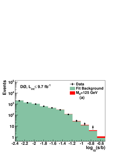
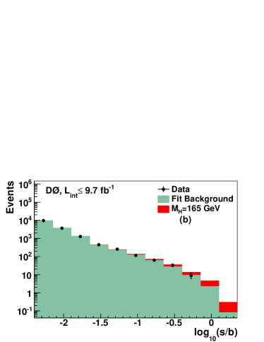
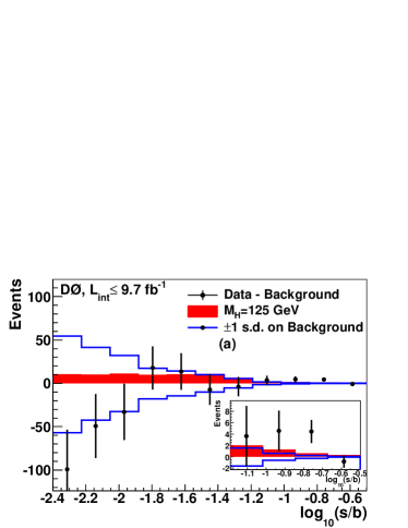
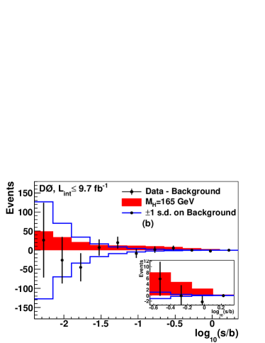
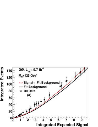
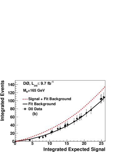
The limit calculation uses the full information available in the individual discriminants. However, for visualization purposes it can be useful to collect all of the inputs into a single distribution. To preserve sensitivity from the bins with high signal-to-background ( $s/b$ ) ratios, where $s$ is the number of signal and $b$ the number of background events, only bins with similar $s/b$ ratio are combined. The aggregate distribution is formed by reordering all of the bins from the input distributions according to $s/b$ ratio. The range of $s/b$ ratio is large, so $\log_{10}(s/b)$ is used. Figure 1 shows the aggregate distributions for $M_{H}=125$ GeV and $M_{H}=165$ GeV, indicating good agreement between data and predictions over several orders of magnitude. Figure 2 shows the same distributions after subtracting the expected background from the data, where solid lines represent the $\pm 1$ standard deviations (s.d.) in systematic uncertainty after a fit to the background-only hypothesis. Integrating the distributions in Fig. 1 from the highest to the lowest $s/b$ events illustrates how the data compare to the $b$ and $s+b$ hypotheses as the events in the highest $s/b$ bins accumulate. Figure 3 shows these cumulative distributions for approximately 150 of the most significant events as a function of the integrated number of signal events. For $M_{H}=125$ GeV, the highest $s/b$ bins contain an excess of signal-like events, while for $M_{H}=165$ GeV, the data follow the background-only expectation.

Refer to caption — Figure 1: (color online) Distributions of $\log_{10}(s/b)$ for data from all contributing channels for (a) $M_{H}=125$ GeV, and (b) $M_{H}=165$ GeV after a fit to data assuming the background-only hypothesis. The data (points with Poisson statistical errors on the expected number of signal+background events) are compared to the expectation from background (light shaded) and signal (dark shaded).

V.2 Systematic Uncertainties

Systematic uncertainties on signal and backgrounds vary among the analyses and they are described in detail in Refs. Abazov:2012wh97 ; Abazov:lvjets ; Abazov:2012kg ; Abazov:2012hv ; Abazov:hWWdilep ; Abazov:2012zj ; Abazov:2013eha ; Abazov:2012ee ; Abazov:hgg . We summarize below only the major components. Most analyses have an uncertainty of 6.1% from the integrated luminosity Andeen:2007zc , while the overall normalizations in the $ZH\rightarrow\ell\ell b\bar{b}$ , $H\rightarrow W^{+}W^{-}\rightarrow\ell^{+}\nu\ell^{-}\bar{\nu}$ , and $VH\rightarrow e^{\pm}\mu^{\pm}$ + $X$ analyses are determined from the mass peak of $Z\rightarrow\ell\ell$ and $Z\rightarrow\tau^{+}\tau^{-}$ decays in data assuming the NNLO $Z/\gamma^{*}$ cross section, reducing the uncertainty to about 1%. The $H\rightarrow b\bar{b}$ analyses have an uncertainty of 1–10% due to the uncertainty on the $b$ -tagging rate, depending on the number and quality of tagged jets. All analyses take into account uncertainties on jet-energy scale, resolution, and jet identification efficiency, for a combined uncertainty of $\approx 7\%$ . All analyses include uncertainties associated with measurement and acceptances of leptons, which range from 1% to 9% depending on the final state. The largest contribution to all analyses is from the uncertainty on the simulated background cross sections which are 4–30% depending on the specific background process. These values include both the uncertainty on the theoretical cross section calculations and the uncertainties on the higher-order correction factors. The uncertainty on the expected multijet background in each channel is dominated by the statistics of the data sample from which it is estimated. It is considered separately from the uncertainties on the simulated backgrounds’ cross sections, and ranges from 10% to 30%. All analyses take into account the uncertainties on the differential cross sections arising from the choice of PDF set and QCD scale. The $H\rightarrow W^{+}W^{-}\rightarrow\ell^{+}\nu\ell^{-}\bar{\nu}$ ( $\ell=e,\mu$ ) analyses divide the data according to jet multiplicity, and consider uncertainties on the contribution from GGF that are a function of jet multiplicity. In addition, several analyses incorporate uncertainties that alter differential distributions and kinematics of the dominant backgrounds in the analyses. These uncertainties are estimated from the variation of the final discriminant distribution due to generator and background modeling uncertainties. Correlations between systematic sources are also carried through in the calculations. For example, the uncertainty on the integrated luminosity is taken to be fully correlated between all signals and backgrounds obtained from simulation. Hence any fluctuation in luminosity is common to all channels for a single pseudoexperiment. All systematic uncertainties originating from a common source are assumed to be fully correlated.

VI Analysis technique validation with diboson production

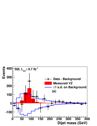
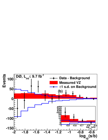
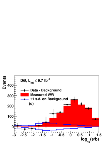
To validate our analyses techniques, we measure diboson production cross sections in the $V+b\bar{b}$ and $\ell\nu\ell\nu$ final states. The analyses use multivariate discriminants that utilize the same input variables as the discriminants used for the Higgs boson search, but with one or more diboson processes acting as the signal. The modified $WH\rightarrow\ell\nu b\bar{b}$ , $ZH\rightarrow\ell\ell b\bar{b}$ , and $ZH\rightarrow\nu\bar{\nu}b\bar{b}$ analyses (collectively called the $VZ$ analyses) treat the $WZ$ and $ZZ$ processes as signal, and the $WW$ process as a background. The Higgs boson processes are not taken into account in this validation procedure. Figure 4(a) shows the background-subtracted data for the dijet invariant mass in the $VZ$ analyses, and Fig. 4(b) for the combined output of the $VZ$ discriminant. Similarly, the modified $H\rightarrow W^{+}W^{-}\rightarrow\ell^{+}\nu\ell^{-}\bar{\nu}$ analysis uses the $WW$ process as the signal with the $WZ$ and $ZZ$ processes as backgrounds. Figure 4(c) shows the background-subtracted data for the output of the $WW$ discriminant. The $VZ$ analyses measure a $WZ+ZZ$ production cross section of $0.73\pm 0.32$ times the SM prediction of 4.4 pb obtained with mcfm. The significance for this measurement to be non-zero is 2.4 s.d. with an expected significance of 3.4 s.d. The $WW$ production cross section is measured to be $1.01\pm 0.06$ times the SM prediction of 11.3 pb, also based on mcfm. Both measurements confirm our ability to extract a small signal from a large background in the same final states, using the same analysis techniques as the search for the Higgs boson, providing validation of the background modeling.

VII Higgs boson results

VII.1 Limits on standard model Higgs boson production

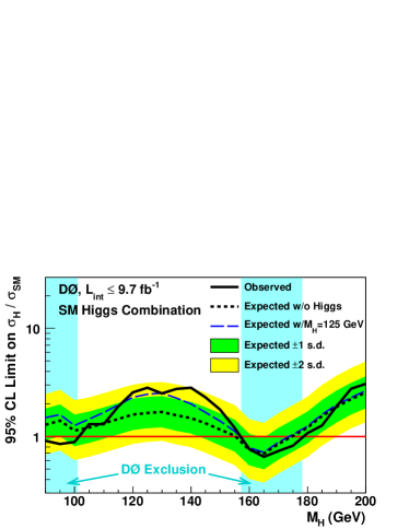
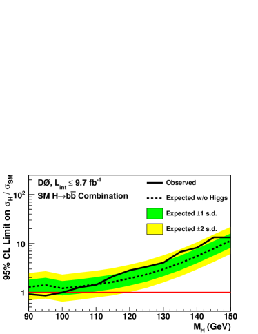
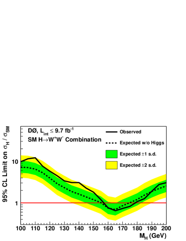
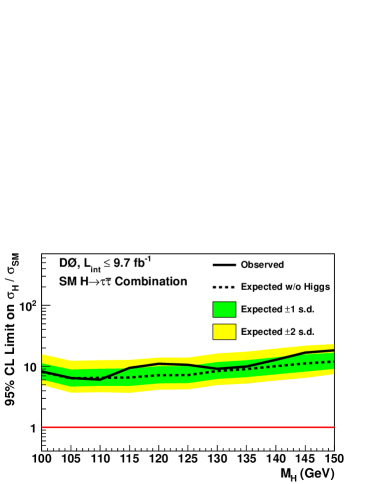
We obtain limits on the product of the Higgs boson production cross section, $\sigma_{H}$ , and branching fractions $\mathcal{B}(H\rightarrow b\bar{b}/W^{+}W^{-}/\tau^{+}\tau^{-}/\gamma\gamma$ ) using individual channels Abazov:2012wh97 ; Abazov:lvjets ; Abazov:2012kg ; Abazov:2012hv ; Abazov:hWWdilep ; Abazov:2012zj ; Abazov:2013eha ; Abazov:2012ee ; Abazov:hgg . We present results in terms of the ratio of the upper limit on $\sigma_{H}$ at 95% C.L. relative to the SM predicted values as a function of $M_{H}$ , where the relative cross sections and branching fractions are kept as predicted by the SM. The SM prediction is therefore excluded at the 95% C.L. for the $M_{H}$ values at which the ratio falls below unity.

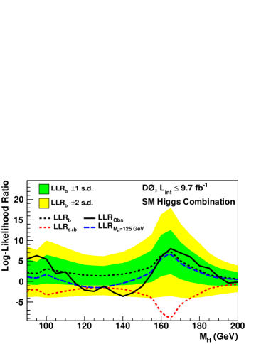
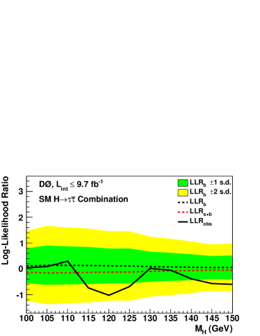
The LLR distributions for the full combination are shown in Fig. 5. Included in these figures are the median LLR values expected for the $s+b$ hypothesis ( $\text{LLR}_{s+b}$ ), $b$ hypothesis ( $\text{LLR}_{b}$ ), and the results observed in data ( $\text{LLR}_{\text{obs}}$ ). The shaded bands represent the $\pm 1$ and $\pm 2~{}\text{s.d}.$ departures for $\text{LLR}_{b}$ . These distributions can be interpreted as follows:

(i)

The separation between $\text{LLR}_{b}$ and $\text{LLR}_{s+b}$ provides a measure of the discriminating power of the search, and illustrates the effectiveness of the analysis to separate the $s+b$ and $b$ hypotheses.
(ii)

The width of the $\text{LLR}_{b}$ distribution (shown here as $\pm 1$ and $\pm 2$ s.d. bands) provides an estimate of the sensitivity of the analysis to a signal-like background fluctuation in the data, taking the systematic uncertainties into account. For example, the sensitivity is limited when a 1 s.d. background fluctuation is large compared to the difference between the $s+b$ and $b$ expectations.
(iii)

The value of $\text{LLR}_{\text{obs}}$ relative to $\text{LLR}_{s+b}$ and $\text{LLR}_{b}$ indicates whether the data distribution appears to be more $s+b$ -like or $b$ -like. The significance of any departures of $\text{LLR}_{\text{obs}}$ from $\text{LLR}_{b}$ can be evaluated through the width of the $\text{LLR}_{b}$ distribution.

As shown in Table 1, only the $WH\rightarrow\ell\nu b\bar{b}$ and $ZH\rightarrow\ell\ell b\bar{b}$ channels contribute to the combination below $M_{H}=100$ GeV. Figure 5 shows that the observed LLR is compatible with the $s+b$ hypothesisfor $120<M_{H}<145$ GeV.

Figure 6 shows the expected and observed upper limits on $\sigma_{H}$ at 95% C.L. relative to the SM, for the mass region $90\leq M_{H}\leq 200$ GeV, for all analyses combined. These results are also summarized in Table 3. We exclude the SM Higgs boson at 95% C.L. in the mass ranges $90<M_{H}<101$ GeV and $157<M_{H}<178$ GeV. Our expected exclusion range is $155<M_{H}<175$ GeV.

Table 3: Expected (median) and observed upper limits on the cross sections relative to the SM at 95% C.L. for the combined analyses for the range

90\leq M_{H}\leq 200

GeV.

$\!M_{H}\!$ (GeV)	90	95	100	105	110	115	120	125	130	135	140	145	150	155	160	165	170	175	180	185	190	195	200
Expected	1.29	1.40	1.13	1.21	1.32	1.45	1.59	1.66	1.69	1.58	1.49	1.33	1.17	1.02	0.75	0.70	0.86	1.02	1.21	1.55	1.89	2.22	2.55
Observed	0.96	0.89	0.95	1.39	1.39	1.99	2.66	2.92	2.56	2.79	2.88	2.36	1.84	1.23	0.78	0.66	0.75	0.85	1.11	1.31	1.96	2.85	3.12

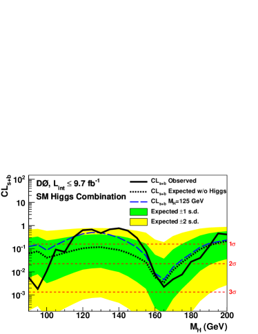
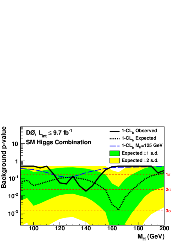
Figure 7 shows the values for the observed $CL_{s+b}$ and its expected behavior as a function of $M_{H}$ . The quantity $CL_{s+b}$ corresponds to the $p$ -value for the $s+b$ hypothesis. Figure 8 shows the quantity $1-CL_{b}$ , which is the $p$ -value for the $b$ hypothesis. These probabilities are local $p$ -values, corresponding to searches for each value of $M_{H}$ separately. These two $p$ -values ( $CL_{s+b}$ and $1-CL_{b}$ ) provide information about the consistency of their respective hypotheses with the observed data at each value of $M_{H}$ . Small values indicate rejection of the hypothesis and values above 50% indicate general agreement between the hypothesis in question and the data. As can be seen in Fig. 7, the observed value of $CL_{s+b}$ drops to $\approx 1\%$ for $M_{H}=160$ GeV, indicating limited consistency with the $s+b$ hypothesis around this mass. In contrast, the observed value of $CL_{s+b}$ is close to unity for $120\leq M_{H}\leq 145$ GeV, whereas $1-CL_{b}$ is small. At $M_{H}=125~{}(140)$ GeV, the value of $1-CL_{b}$ is $4.1\%$ ( $1.8\%$ ), corresponding to $1.7$ ( $2.1$ ) s.d. above the background prediction.

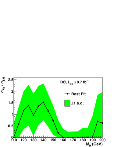
As a further investigation of this excess, we present in Fig. 9 the best fit of the data to the ratio of $\sigma_{H}$ to the SM prediction ( $\sigma_{\text{Fit}}/\sigma_{\text{SM}}$ ). The result of this fit, shown along with its band of $\pm 1~{}$ s.d., yields a signal rate of approximately a factor of 1.4 larger than the SM cross section for $M_{H}$ between 120 GeV and 145 GeV. For $M_{H}=125$ GeV, we obtain a ratio of $1.4\pm 0.9$ . The associated production analyses with $H\to b\bar{b}$ decay and the $H\rightarrow W^{+}W^{-}\rightarrow\ell^{+}\nu\ell^{-}\bar{\nu}$ analyses dominate our sensitivity. The dijet invariant mass resolution is approximately 15% for associated production with $H\to b\bar{b}$ decay. The mass resolution for the analyses with $H\to W^{+}W^{-}$ decay is poor due to the undetected neutrinos in the final state. We therefore expect a Higgs boson signal to appear as a broad excess over background, rather than a narrow resonance such as that expected at the LHC in the $H\to\gamma\gamma$ or $H\to ZZ\to 4\ell$ final states.

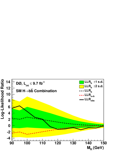
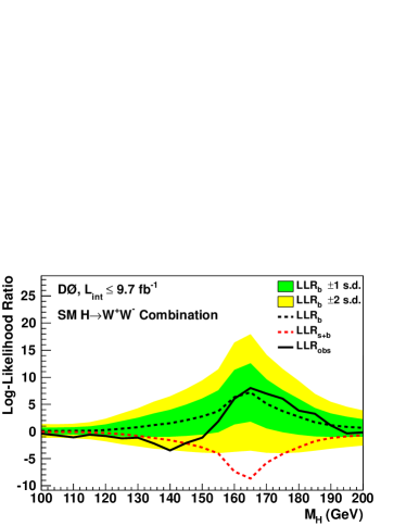
We study the excess at low mass by separating the major contributing sources according to the Higgs boson decay: $H\rightarrow b\bar{b}$ , $H\rightarrow W^{+}W^{-}$ , $H\rightarrow\tau^{+}\tau^{-}$ and $H\rightarrow\gamma\gamma$ final states. Figure 10 shows the LLR values from the combination of the results from the $ZH\rightarrow\ell\ell b\bar{b}$ , $ZH\rightarrow\nu\nu b\bar{b}$ and $WH\rightarrow\ell\nu b\bar{b}$ searches, and illustrates a small excess that is compatible with the SM Higgs boson expected rate for $120\leq M_{H}\leq 145$ GeV. Figure 11 shows the LLR values from the combination of the results from searches for $H\rightarrow W^{+}W^{-}\rightarrow\ell\nu\ell\nu$ , $H\rightarrow W^{+}W^{-}\rightarrow\ell\nu jj$ , and $VH\rightarrow VWW$ , together with the $WW$ -dominated subchannels from the $H+X\rightarrow\ell\tau_{h}jj$ analysis, and shows a similar excess of data over the background for $110\leq M_{H}\leq 150$ GeV. At higher masses, where the Tevatron sensitivity to Higgs boson production is the largest, the LLR favors the $b$ hypothesis. Figure 12 shows the LLR values from the combination of the $\tau\tau$ -dominated $H+X\rightarrow\ell\tau_{h}jj$ subchannels and the $VH\rightarrow\tau_{h}\tau_{h}\mu+X$ analysis, in which a significant fraction of the Higgs boson decays are to $\tau^{+}\tau^{-}$ pairs. Figures 13–15, as well as Tables 4–6, show the expected and observed 95% C.L. cross section limits in terms of ratio to the SM predictions

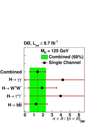
for $H\rightarrow b\bar{b}$ , $H\rightarrow W^{+}W^{-}$ , and $H\rightarrow\tau^{+}\tau^{-}$ final states, respectively. The corresponding figures for the $H\rightarrow\gamma\gamma$ analysis can be found in Ref. Abazov:hgg . Figure 16 shows the best fit of the ratio $\sigma_{H}\cdot\mathcal{B}/(\sigma_{H}\cdot\mathcal{B})_{SM}$ for $M_{H}=125$ GeV in each of the Higgs boson decay channels considered, as well as the central value for all analyses combined. These values are also given in Table 7.

Table 4: Expected (median) and observed upper limits for

\sigma\times\mathcal{B}(H\rightarrow b\bar{b})

relative to the SM at 95% C.L. for the combined

WH/ZH,H\rightarrow b\bar{b}

analyses for the range

90\leq M_{H}\leq 150

GeV.

$M_{H}$ (GeV)	90	95	100	105	110	115	120	125	130	135	140	145	150
Expected	1.29	1.40	1.21	1.31	1.45	1.63	1.92	2.33	2.99	3.96	5.52	7.91	11.35
Observed	0.96	0.89	1.05	1.33	1.51	2.25	2.96	3.49	4.29	6.92	8.65	13.85	13.90

Table 5: Expected (median) and observed upper limits for

\sigma\times\mathcal{B}(H\rightarrow W^{+}W^{-})

relative to the SM at 95% C.L. for the combined

WH/ZH/H,H\rightarrow W^{+}W^{-}

analyses for the range

100\leq M_{H}\leq 200

GeV.

$M_{H}$ (GeV)	100	105	110	115	120	125	130	135	140	145	150	155	160	165	170	175	180	185	190	195	200
Expected	7.25	7.09	6.49	5.34	3.97	2.92	2.33	1.88	1.64	1.40	1.20	1.02	0.75	0.70	0.86	1.02	1.21	1.55	1.89	2.22	2.55
Observed	9.98	11.69	12.38	7.70	5.84	4.55	3.42	3.15	3.14	2.30	1.86	1.23	0.78	0.66	0.75	0.85	1.11	1.31	1.96	2.85	3.12

Table 6: Expected (median) and observed upper limits for

\sigma\times\mathcal{B}(H\rightarrow\tau^{+}\tau^{-})

relative to the SM at 95% C.L. for the combined

VH\rightarrow\tau_{h}\tau_{h}\mu+X

and

H+X\rightarrow\ell\tau_{h}jj

analyses for the range

100\leq M_{H}\leq 150

GeV.

$M_{H}$ (GeV)	100	105	110	115	120	125	130	135	140	145	150
Expected	8.22	6.39	6.54	6.59	7.21	7.25	8.46	9.05	10.11	11.28	12.11
Observed	8.42	6.64	6.20	9.70	11.29	10.84	9.35	10.17	13.07	17.16	18.59

Table 7: The best fit Higgs boson cross section times branching fraction as a ratio to the SM cross section times branching fraction for

M_{H}=125

GeV for the individual combinations according to Higgs boson decay mode, as well as the full combination.

Combined	$1.40^{+0.92}_{-0.88}$
$H\rightarrow\gamma\gamma$	$4.20^{+4.60}_{-4.20}$
$H\rightarrow W^{+}W^{-}$	$1.90^{+1.63}_{-1.52}$
$H\rightarrow\tau^{+}\tau^{-}$	$3.96^{+4.11}_{-3.38}$
$H\rightarrow b\bar{b}$	$1.23^{+1.24}_{-1.17}$

VII.2 Interpretation in fourth generation and Fermiophobic Higgs boson models

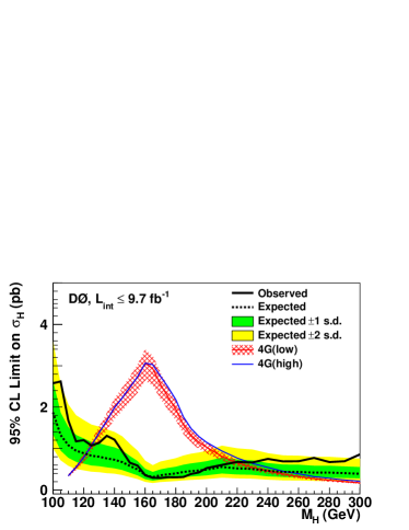
We also interpret our Higgs boson searches in models containing a fourth generation of fermions, and models with a fermiophobic Higgs boson. The fourth generation models Holdom:2009rf feature a modified $Hgg$ coupling, leading to a nearly order of magnitude enhancement in the GGF cross section relative to the SM Arik:2005ed ; Kribs:2007nz ; Anastasiou:2010bt . Previous interpretations of SM Higgs boson searches within the context of a fourth generation of fermions at the Fermilab Tevatron Collider exclude $131<M_{H}<207$ GeV Aaltonen:2010sv . Both ATLAS Aad:2011qi and CMS CMS-SM4 have performed similar searches, which exclude, respectively, $140<M_{H}<185$ GeV and $110<M_{H}<600$ GeV. Although the larger coupling increases the decay width to $gg$ , the $WW^{*}$ decay mode remains dominant for $M_{H}>135$ GeV. There is also a small contribution from $H\rightarrow ZZ^{*}\rightarrow\ell\ell\nu\nu$ production that increases with $M_{H}$ . We consider two fourth generation scenarios: (i) a “low mass” scenario in which the mass of the fourth generation neutrino is set to $m_{\nu 4}=80$ GeV, and the mass of the fourth generation charged lepton $m_{\ell 4}$ is set to 100 GeV, and (ii) a “high mass” scenario in which $m_{\nu 4}=m_{\ell 4}=1$ TeV, so that the fourth generation leptons do not affect the decay branching fractions of the Higgs boson. In both scenarios the fourth generation quark masses are set to be those of the high mass scenario in Ref. Anastasiou:2010bt .

We consider only $gg\rightarrow H$ production and the $H\rightarrow W^{+}W^{-}\rightarrow\ell^{+}\nu\ell^{-}\bar{\nu}$ and $H\rightarrow W^{+}W^{-}\rightarrow\ell\nu q^{\prime}\bar{q}$ $(qq)$ channels to set limits on the fourth generation models, and also set a limit on $\sigma(gg\to H)\times\mathcal{B}(H\to W^{+}W^{-})$ . We scale the product of the cross sections and branching fractions to the results from hdecay, modified to include the fourth generation. We retrain our multivariate discriminants to take only the above signals into account, and do not include events with two or more jets in the $H\rightarrow W^{+}W^{-}\rightarrow e\nu e\nu/\mu\nu\mu\nu$ analyses. We also do not include the theoretical uncertainty on $\sigma(gg\to H)\times\mathcal{B}(H\to W^{+}W^{-})$ since the absolute cross section limits do not depend on the prediction. We include the theoretical uncertainties for limits on ratios to cross sections.

Figure 17 shows the combined limits on $\sigma(gg\to H)\times\mathcal{B}(H\to W^{+}W^{-})$ , along with the fourth generation theory predictions for the high mass and low mass scenarios. We exclude a SM-like Higgs boson in the range $125<M_{H}<218$ GeV at 95% C.L., with an expected exclusion range of $122<M_{H}<232$ GeV in the low mass scenario. In the high mass scenario, the observed (expected) exclusion range is $125<M_{H}<228$ ( $122<M_{H}<251$ ) GeV.

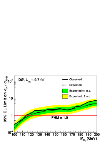
In the fermiophobic model (FHM), the lightest Higgs boson $H_{f}$ couplings to fermions vanish at leading order, but otherwise $H_{f}$ is like the SM Higgs boson. Hence, $gg\to H_{f}$ production is negligible, and $H_{f}$ decays to fermions are forbidden, but $V+H_{f}$ and vector boson fusion $q\bar{q}\rightarrow q^{\prime}\bar{q}^{\prime}H_{f}$ production remain nearly unchanged relative to the SM. The $WW$ , $ZZ$ , $\gamma\gamma$ , and $Z\gamma$ decays comprise nearly the entire decay width. For all $M_{H_{f}}$ the $H_{f}\to W^{+}W^{-}$ decay has the largest branching fraction. The $H_{f}\to\gamma\gamma$ branching fraction is greatly enhanced over the SM for all $M_{H_{f}}$ , and it provides most of the search sensitivity for $M_{H_{f}}<120$ GeV.

The CDF and D0 Collaborations have previously published results in the $H_{f}\to\gamma\gamma$ decay channel Collaboration:2012pa ; Abazov:2011ix . The analyses described here supersede previous FHM searches at D0. The ATLAS and CMS Collaborations have performed fermiophobic searches, and exclude $110<M_{H_{f}}<118.0$ GeV, $119.5<M_{H_{f}}<121.0$ GeV Aad:2012yq , and $110<M_{H_{f}}<147$ GeV CMS-SM4 using $\gamma\gamma$ final states, and $110<M_{H_{f}}<194$ GeV when other final states are included CMS:2012bd .

We combine the $H\to\gamma\gamma$ and $H\to W^{+}W^{-}$ decay channels, produced either in association with a $V$ boson, or in VBF, for the FHM interpretation. We reoptimize the SM $H\rightarrow\gamma\gamma$ analysis to take into account the different kinematics in the FHM, e.g., the presence of an associated vector boson in the FHM, or recoiling quark jets in VBF, which shift the transverse momentum spectrum of the Higgs boson to higher values than in the SM. Likewise, we retrain the multivariate discriminants for the $H\rightarrow W^{+}W^{-}\rightarrow(e^{+}e^{-},\mu^{+}\mu^{-},e^{\pm}\mu^{\mp})\nu\bar{\nu}$ analyses to account for the suppressed GGF process in the FHM. We retain the existing subdivision into categories that are based on the number of reconstructed jets in the event. The other SM $H\to WW$ analyses can be interpreted directly in the FHM without reoptimization, after separating the relative contributions from GGF, $WH$ , $ZH$ , and VBF in each contributing channel, removing the GGF component, and scaling the remaining signal contributions by the ratio of the branching fraction in the FHM and SM, $\mathcal{B}(H_{f}\to WW)/\mathcal{B}(H_{SM}\to WW)$ . Figure 18 shows the combined FHM limits. The observed (expected) 95% C.L. exclusion range is $100<M_{H_{f}}<114$ ( $100<M_{H_{f}}<117$ ) GeV.

VIII Conclusions

We have presented a combination of searches for SM Higgs boson production with the D0 experiment using data corresponding to up to $9.7$ fb^-1 of $p\bar{p}$ collisions at $\sqrt{s}=1.96$ TeV. We set upper limits on the production cross section at 95% C.L. for Higgs boson masses of $90<M_{H}<200$ GeV. We also interpret the searches in terms of models containing a fourth generation of fermions, as well as models with a fermiophobic Higgs boson ( $H_{f}$ ) having suppressed couplings to fermions. We exclude a Higgs boson in the mass range $125<M_{H}<218$ ( $125<M_{H}<228$ ) GeV, in the low mass (high mass) fourth generation scenario, and a fermiophobic Higgs boson with a mass $100<M_{H_{f}}<114$ GeV. The observed upper limits on SM Higgs boson production are $2.86~{}(0.66)\times\sigma_{\text{SM}}$ at $M_{H}=125~{}(165)$ GeV, with an expected limit of $1.68~{}(0.70)\times\sigma_{\text{SM}}$ . We exclude the regions of $90<M_{H}<101$ GeV and $157<M_{H}<178$ GeV with an a priori expected exclusion of $155<M_{H}<175$ GeV. In the range of $M_{H}\approx 120-145$ GeV, the data exhibit an excess above the background prediction of up to two standard deviations consistent with the presence of a 125 GeV SM Higgs boson. Each of the four main Higgs boson decay mode combinations contributes to this excess. The analyses combined here also provide inputs to the overall Tevatron combination Aaltonen:2013kxa , which reports an excess in data at the level of 3 standard deviations, consistent with the production of a 125 GeV SM Higgs boson in final states corresponding to its expected decay modes.

Acknowledgements.

We thank the staffs at Fermilab and collaborating institutions, and acknowledge support from the DOE and NSF (USA); CEA and CNRS/IN2P3 (France); MON, NRC KI and RFBR (Russia); CNPq, FAPERJ, FAPESP and FUNDUNESP (Brazil); DAE and DST (India); Colciencias (Colombia); CONACyT (Mexico); NRF (Korea); FOM (The Netherlands); STFC and the Royal Society (United Kingdom); MSMT and GACR (Czech Republic); BMBF and DFG (Germany); SFI (Ireland); The Swedish Research Council (Sweden); and CAS and CNSF (China).

References

(1) P. W. Higgs, Phys. Lett. 12, 132 (1964).
(2) F. Englert and R. Brout, Phys. Rev. Lett. 13, 321 (1964).
(3) P. W. Higgs, Phys. Rev. Lett. 13, 508 (1964).
(4) G. S. Guralnik, C. R. Hagen, and T. W. B. Kibble, Phys. Rev. Lett. 13, 585 (1964).
(5) T. Aaltonen et al., [CDF Collaboration], Phys. Rev. Lett. 108, 151803 (2012).
(6) V. M. Abazov et al., [D0 Collaboration], Phys. Rev. Lett. 108, 151804 (2012).
(7) T. Aaltonen et al., [CDF and D0 Collaboration], Phys. Rev. D 86, 092003 (2012).
(8) LEP Electroweak Working Group, Status as of March 2012, http://lepewwg.web.cern.ch/LEPEWWG/.
(9) R. Barate et al., (LEP Working Group for Higgs boson searches), Phys. Lett. B 565, 61 (2003).
(10) TEVNPH (Tevatron New Phenomena and Higgs Working Group), arXiv:1203.3774, (2012).
(11) T. Aaltonen et al., [CDF and D0 Collaboration], Phys. Rev. D 82, 011102 (2010).
(12) G. Aad et al., [ATLAS Collaboration], Phys. Rev. D 86, 032003 (2012).
(13) S. Chatrchyan et al., [CMS Collaboration], Phys. Lett. B 710, 26 (2012).
(14) G. Aad et al., [ATLAS Collaboration], Phys. Lett. B 716, 1 (2012).
(15) S. Chatrchyan et al., [CMS Collaboration], Phys. Lett. B 716, 30 (2012).
(16) T. Aaltonen et al., [CDF and D0 Collaboration], Phys. Rev. Lett. 109, 071804 (2012).
(17) S. Abachi et al., [D0 Collaboration], Nucl. Instrum. Methods Phys. Res. A 338, 185 (1994).
(18) V. M. Abazov et al., [D0 Collaboration], Nucl. Instrum. Methods Phys. Res. A 565, 463 (2006).
(19) M. Abolins et al., Nucl. Instrum. Methods Phys. Res. A 584, 75 (2008).
(20) R. Angstadt et al., Nucl. Instrum. Methods Phys. Res. A 622, 298 (2010).
(21) V. M. Abazov et al., [D0 Collaboration], Phys. Rev. Lett. 109, 121804 (2012).
(22) V. M. Abazov et al., [D0 Collaboration], Phys. Rev. D 88, 052008 (2013).
(23) V. M. Abazov et al., [D0 Collaboration], Phys. Rev. Lett. 109, 121803 (2012).
(24) V. M. Abazov et al., [D0 Collaboration], Phys. Rev. D 88, 052010 (2013).
(25) V. M. Abazov et al., [D0 Collaboration], Phys. Lett. B 716, 285 (2012).
(26) V. M. Abazov et al., [D0 Collaboration].
(27) V. M. Abazov et al., [D0 Collaboration], Phys. Lett. B 714, 237 (2012).
(28) V. M. Abazov et al., [D0 Collaboration], Phys. Rev. D 88, 052009 (2013).
(29) V. M. Abazov et al., [D0 Collaboration], Phys. Rev. D 88, 052005 (2013).
(30) V. M. Abazov et al., [D0 Collaboration], Phys. Rev. D 88, 052007 (2013).
(31) V. M. Abazov et al., [D0 Collaboration], Nucl. Instrum. Methods Phys. Res. A 620, 490 (2010).
(32) V. M. Abazov et al., [D0 Collaboration], Phys. Rev. Lett. 109, 121802 (2012).
(33) I. Narsky, arXiv:physics/0507157, (2005).
(34) L. Breiman, J. H. Friedman, R. A. Olshen, and C. J. Stone, Classification and Regression Trees (Wadsworth & Brooks/Cole Advanced Books and Software, Pacific Grove, CA, 1984).
(35) R. E. Schapire, The Boosting Approach to Machine Learning: An Overview, MSRI Workshop on Nonlinear Estimation and Classification, Berkeley, CA, USA, 2001.
(36) Y. Freund and R. E. Schapire, J. Japanese Society for Artificial Intelligence 14, 771 (1999).
(37) J. H. Friedman, eConf C030908, WEAT003 (2003).
(38) A. Hoecker et al., PoS ACAT, 040 (2007), we use version 4.1.0.
(39) T. Sjöstrand, S. Mrenna, and P. Z. Skands, J. High Energy Phys. 05, 026 (2006).
(40) M. L. Mangano, M. Moretti, F. Piccinini, R. Pittau, and A. D. Polosa, J. High Energy Phys. 07, 001 (2003).
(41) T. Gleisberg et al., J. High Energy Phys. 02, 007 (2009).
(42) E. Boos et al., Nucl. Instrum. Methods Phys. Res. A 534, 250 (2004).
(43) E. E. Boos, V. E. Bunichev, L. V. Dudko, V. I. Savrin, and V. V. Sherstnev, Phys. Atom. Nucl. 69, 1317 (2006).
(44) H. L. Lai et al., Phys. Rev. D 55, 1280 (1997).
(45) P. M. Nadolsky et al., Phys. Rev. D 78, 013004 (2008).
(46) R. Hamberg, W. L. van Neerven, and T. Matsuura, Nucl. Phys. B 359, 343 (1991), ibid, B 644, 403 (2002).
(47) J. M. Campbell and R. K. Ellis, Phys. Rev. D 60, 113006 (1999).
(48) J. M. Campbell, R. K. Ellis, and C. Williams, MCFM - Monte Carlo for FeMtobarn processes, http://mcfm.fnal.gov/.
(49) U. Langenfeld, S. Moch, and P. Uwer, Phys. Rev. D 80, 054009 (2009).
(50) N. Kidonakis, Phys. Rev. D 74, 114012 (2006).
(51) V. M. Abazov et al., [D0 Collaboration], Phys. Rev. Lett. 100, 102002 (2008).
(52) K. Melnikov and F. Petriello, Phys. Rev. D 74, 114017 (2006).
(53) T. Melia, P. Nason, R. Rontsch, and G. Zanderighi, J. High Energy Phys. 1111, 078 (2011).
(54) G. Bozzi, S. Catani, D. de Florian, and M. Grazzini, Phys. Lett. B 564, 65 (2003).
(55) G. Bozzi, S. Catani, D. de Florian, and M. Grazzini, Nucl. Phys. B 737, 73 (2006).
(56) D. de Florian, G. Ferrera, M. Grazzini, and D. Tommasini, J. High Energy Phys. 11, 064 (2011).
(57) C. Balazs, J. Huston, and I. Puljak, Phys. Rev. D 63, 014021 (2001).
(58) Q.-H. Cao, C.-R. Chen, C. Schmidt, and C.-P. Yuan, arXiv:0909.2305, (2009).
(59) C. Anastasiou, R. Boughezal, and F. Petriello, J. High Energy Phys. 04, 003 (2009).
(60) D. de Florian and M. Grazzini, Phys. Lett. B 674, 291 (2009).
(61) M. Grazzini, 2010, private communication.
(62) TEVEWG (Tevatron Electroweak Working Group), arXiv:0903.2503, (2009).
(63) R. V. Harlander and W. B. Kilgore, Phys. Rev. Lett. 88, 201801 (2002).
(64) C. Anastasiou and K. Melnikov, Nucl. Phys. B 646, 220 (2002).
(65) V. Ravindran, J. Smith, and W. L. van Neerven, Nucl. Phys. B 665, 325 (2003).
(66) S. Actis, G. Passarino, C. Sturm, and S. Uccirati, Phys. Lett. B 670, 12 (2008).
(67) U. Aglietti, R. Bonciani, G. Degrassi, and A. Vicini, arXiv:hep-ph/0610033, (2006).
(68) S. Catani, D. de Florian, M. Grazzini, and P. Nason, J. High Energy Phys. 07, 028 (2003).
(69) A. D. Martin, W. J. Stirling, R. S. Thorne, and G. Watt, Eur. Phys. J. C 64, 653 (2009).
(70) S. Alekhin et al., arXiv:1101.0536, (2011).
(71) M. Botje et al., arXiv:1101.0538, (2011).
(72) I. W. Stewart and F. J. Tackmann, Phys. Rev. D 85, 034011 (2012).
(73) C. Anastasiou, G. Dissertori, M. Grazzini, F. Stockli, and B. R. Webber, J. High Energy Phys. 08, 099 (2009).
(74) J. M. Campbell, R. K. Ellis, and C. Williams, Phys. Rev. D 81, 074023 (2010).
(75) J. Baglio and A. Djouadi, J. High Energy Phys. 10, 064 (2010).
(76) M. Spira, Fortran codes, http://people.web.psi.ch/spira/proglist.html.
(77) O. Brein, A. Djouadi, and R. Harlander, Phys. Lett. B 579, 149 (2004).
(78) M. L. Ciccolini, S. Dittmaier, and M. Kramer, Phys. Rev. D 68, 073003 (2003).
(79) P. Bolzoni, F. Maltoni, S.-O. Moch, and M. Zaro, Phys. Rev. D 85, 035002 (2012).
(80) A. Djouadi, J. Kalinowski, and M. Spira, Comput. Phys. Commun. 108, 56 (1998), We use hdecay Version 3.53.
(81) J. M. Butterworth et al., arXiv:1003.1643, (2010).
(82) J. Baglio and A. Djouadi, J. High Energy Phys. 03, 055 (2011).
(83) T. Junk, Nucl. Instrum. Methods Phys. Res. A 434, 435 (1999).
(84) A. L. Read, J. Phys. G 28, 2693 (2002).
(85) W. Fisher, FERMILAB-TM-2386-E (2007).
(86) T. Andeen et al., FERMILAB-TM-2365 (2007).
(87) B. Holdom et al., PMC Phys. A3, 4 (2009), 0904.4698.
(88) E. Arik, O. Cakir, S. A. Cetin, and S. Sultansoy, Acta Phys. Polon. B 37, 2839 (2006).
(89) G. D. Kribs, T. Plehn, M. Spannowsky, and T. M. P. Tait, Phys. Rev. D 76, 075016 (2007).
(90) C. Anastasiou, R. Boughezal, and E. Furlan, J. High Energy Phys. 06, 101 (2010).
(91) G. Aad et al., [ATLAS Collaboration], Eur. Phys. J. C 71, 1728 (2011).
(92) S. Chatrchyan et al., [CMS Collaboration], arXiv:1302.1764, (2013), submitted to Phys. Lett. B.
(93) T. Aaltonen et al., [CDF Collaboration], Phys. Lett. B 717, 173 (2012).
(94) V. M. Abazov et al., [D0 Collaboration], Phys. Rev. Lett. 107, 151801 (2011).
(95) G. Aad et al., [ATLAS Collaboration], Eur. Phys. J. C 72, 2157 (2012).
(96) S. Chatrchyan et al., [CMS Collaboration], J. High Energy Phys. 09, 111 (2012).
(97) T. Aaltonen et al., [CDF and D0 Collaboration], Phys. Rev. D 88, 052014 (2013).

Combined search for the Higgs boson with the D0 experiment

Abstract

pacs:

I Introduction

II Contributing Analyses

II.1 H→b​b¯→𝐻𝑏¯𝑏H\rightarrow b\bar{b} Analyses

II.2 H→W​W∗→𝐻𝑊superscript𝑊H\rightarrow WW^{*} Analyses

II.3 H→τ+​τ−→𝐻superscript𝜏superscript𝜏H\rightarrow\tau^{+}\tau^{-} and H→γ​γ→𝐻𝛾𝛾H\rightarrow\gamma\gamma analyses

III Background Estimation

IV Signal Predictions and Uncertainties

V Limit Calculations

V.1 Final Variable Distributions

V.2 Systematic Uncertainties

VI Analysis technique validation with diboson production

VII Higgs boson results

VII.1 Limits on standard model Higgs boson production

VII.2 Interpretation in fourth generation and Fermiophobic Higgs boson models

VIII Conclusions

Acknowledgements.

References

II.1 $H\rightarrow b\bar{b}$ Analyses

II.2 $H\rightarrow WW^{*}$ Analyses

II.3 $H\rightarrow\tau^{+}\tau^{-}$ and $H\rightarrow\gamma\gamma$ analyses