Spatial partitioning improves the reliability of biochemical signaling
Abstract
Spatial heterogeneity is a hallmark of living systems, even at the molecular scale in individual cells. A key example is the partitioning of membrane-bound proteins via lipid domain formation or cytoskeleton-induced corralling. Yet the impact of this spatial heterogeneity on biochemical signaling processes is poorly understood. Here we demonstrate that partitioning improves the reliability of biochemical signaling. We exactly solve a stochastic model describing a ubiquitous motif in membrane signaling. The solution reveals that partitioning improves signaling reliability via two effects: it moderates the non-linearity of the switching response, and it reduces noise in the response by suppressing correlations between molecules. An optimal partition size arises from a trade-off between minimizing the number of proteins per partition to improve signaling reliability and ensuring sufficient proteins per partition to maintain signal propagation. The predicted optimal partition size agrees quantitatively with experimentally observed systems. These results persist in spatial simulations with explicit diffusion barriers. Our findings suggest that molecular partitioning is not merely a consequence of the complexity of cellular substructures, but also plays an important functional role in cell signaling.
The cell membrane is a nexus of information processing. Once regarded as a simple barrier between a cell and its surroundings, it is now clear that the membrane is a hotspot of molecular activity, where signals are integrated and modulated even before being relayed to the inside of the cell [1]. Moreover, the membrane itself is structurally complex. Regions enriched in glycosphingolipids, cholesterol, and other membrane components, often called lipid rafts, transiently assemble and float within the surrounding bilayer [2], providing platforms for molecular interaction [3]. Additionally, interaction of the membrane with the underlying actin cytoskeleton forms compartments in which molecules are transiently trapped [4, 5]. These membrane sub-domains create a highly heterogeneous environment in which molecules are far from well mixed, and it is currently unclear what effect this heterogeneity has on cell signaling.
Membrane sub-domains are thought to play a dominant role in the observed aggregation of signaling molecules into clusters [6]. Interestingly, these clusters have a characteristic size of only a few molecules. For example, the GPI-anchored receptor CD59 is observed to form clusters of three to nine molecules upon interaction with the cytoskeleton and lipid rafts [7, 8]. Similarly, the well-studied membrane-bound GTPase Ras forms clusters of six to eight molecules which also depend on interactions with the cytoskeleton and rafts [9, 10]. Despite the important findings that aggregation of proteins induced by sub-domains can affect reaction kinetics [11], enhance oligomerization [1], modulate downstream responses [12, 13] and enhance signal fidelity [13, 14], the origin of this characteristic size remains unknown. While it is quite possible that these domains owe their size to a thermodynamic or structural origin, we here address the question of whether this size can be optimized for signaling performance. We find that the partitioning imposed by sub-domains gives rise to a trade-off in cell signaling, from which an optimal size of a few molecules emerges naturally, suggesting that reliable signaling is intimately tied to the spatial structure of the membrane.
We study via stochastic analysis and spatial simulation a model that is directly motivated by both CD59 and Ras signaling at the membrane. Stimulated CD59 receptors induce the switching of several Src-family kinases from an unphosphorylated to a phosphorylated state [7, 8]. Similarly, stimulated EGF receptors induce the switching of Ras proteins from an inactive GDP-loaded state to an active GTP-loaded state [13]. We therefore study the simple and ubiquitous motif of coupled switching reactions, in which the activation of one species (the receptor) triggers the activation of a second species (the downstream effector).
We exactly solve this stochastic model of coupled switching reactions, and we use the solution to compare signaling reliability in a spatially-partitioned system to that in a well-mixed system. We demonstrate that partitioning can improve signaling performance by generating a more graded input-output relation and by reducing the noise in the signaling response. This latter effect comes about because partitioning reduces the correlations between the states of the different output molecules. On the other hand, the stochastic exchange of proteins between partitions can generate configurations which isolate molecules and exclude them from the signaling process, thereby reducing the dynamic range of the response and increasing the output noise. The trade-off between these two effects results in an optimal partition size that agrees well with cluster sizes of signaling proteins that are observed experimentally [7, 8, 9, 10], suggesting that cluster sizes are tuned so as to maximize information transmission.
1 Results
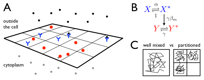
We model two coupled molecular species at the membrane, as depicted in Fig. 1A. A membrane-bound receptor (e.g. CD59 or EGF receptor) is activated via ligand stimulation, and the active receptor in turn activates a membrane-bound effector (e.g. a Src-family kinase or Ras). A reaction scheme representing these processes is shown in Fig. 1B, and consists of two protein species: the receptor and the downstream effector . The switching of molecules from the to the state is driven by an external signal of strength . Active molecules act on inactive molecules and promote switching to the state. Deactivation of both active protein species occurs spontaneously and independently.
We will be concerned with how the network response, the number of active molecules as a function of the input signal , is affected by the spatial structure of the system. In particular we ask how partitioning of the reaction system into non-interacting sub-domains affects the reliability of signal transmission, which is determined by two principal factors: the input-output response and the output noise; together these properties determine to what extent different input signals can be reliably resolved from the network response. We focus on two system configurations, shown in Fig. 1C. In the first case we assume that all molecules are present in a single well-mixed reaction compartment. In the second case, we consider a system partitioned into compartments between which no interactions are permitted; here we take the output of the system to be the total number of active molecules in all compartments. This choice of output corresponds to a readout of the signal by, e.g., a cytosolic component whose diffusion is much faster than the diffusion and signaling of and on the membrane. In the partitioned system, we will for simplicity first assume that the molecules are uniformly and statically distributed among compartments. However, recognizing that this scenario will not generally be realized inside cells, we will later relax this assumption and consider exchange of molecules among partitions.
We model the dynamics of the well-mixed system, as well as each compartment within the partitioned system, using a stochastic equation of the same form. We denote the total numbers of and molecules by and , respectively, and the numbers of active and molecules by and , respectively. To parameterize the system, we scale units of time by the deactivation rate of , such that the effective deactivation rate is . Then denotes the rescaled activation rate of ; is the rate of deactivation of relative to that of ; and is the activation rate of a given molecule for a particular concentration of molecules. The parameter incorporates the effective strength of the input signal and determines the mean activity via the occupancy . The precise -dependence of the coupling function will depend on the exact nature of the interactions between and molecules. We take , with the volume of the compartment in which the reactions are taking place. However, our conclusions are unaffected if we instead take a Michaelis-Menten form (Appendix C: Fig. 7). The total system volume is assumed to scale with the total number of molecules, such that is constant. The coupling function in partition is then determined by , the number of molecules in partition , according to for constant .
The probability of having proteins in the state and proteins in the state evolves according to the chemical master equation (CME),
| (1) |
subject to suitable boundary conditions. The nature of the particular set of reactions in our model (Fig. 1B) means that the operators and have the same form,
| (2) |
where defines the step operator. Despite the appearance of terms containing the product in the operator , which make the direct calculation of moments of from the CME impossible, an exact solution to (1) can be found for arbitrary using the method of spectral expansion [15, 16] as described in Appendix A.1.
1.1 Partitioning leads to a more graded response
We begin by analyzing the behavior of a minimal system with . In the well-mixed system, all molecules are contained within domain of volume . In the partitioned system, subdomains with volume each contain one and one molecule.
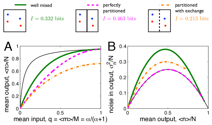
We first focus on the mean response . In the limits of small or large the mean response is the same in both the partitioned and mixed systems, and respectively. However, at all intermediate values of , the mean response of the well-mixed system is larger than that of the partitioned system; equivalently, the partitioned system exhibits a more graded response than the well-mixed system to changes in the input signal (see Fig. 2A, thick solid and dashed curves). The more graded response is due to higher fluctuations in activity. When or , all molecules are inactive or active, respectively; however at intermediate values of , the number of active molecules fluctuates. Partitioning reduces the number of molecules per reaction compartment, increasing the relative size of these fluctuations according to . These fluctuations are passed through the concave dependence of on , resulting in a smaller mean (via Jensen’s inequality [17]), and therefore a more linear response curve (see also Appendix C: Fig. 8A).
A more graded input-output relation can potentially enhance signaling by expanding the range of input signals which the network is able to transmit without saturating the response. However, in order to determine whether this larger input range can be resolved in the network it is crucial to examine how the noise in the response is affected.
1.2 Partitioning reduces noise
Figure 2B shows the variance of the output as a function of the mean response for the system with , as the input signal strength is varied. We see that the output noise is reduced in the partitioned system relative to the well-mixed system across the full range of response levels. The noise reduction is surprising: one might expect that the increased fluctuations in activity that come with partitioning would propagate to fluctuations in activity. Indeed, this is the case: in a single compartment, as the number of molecules is reduced, the noise in the output increases (Appendix C: Fig. 8B). However, this effect is overcome by a second effect: partitioning reduces correlations among output molecules.
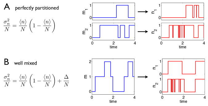
To see the effect of partitioning on correlations, we consider the expressions for the variance. In the partitioned case, since the two molecules switch independently, the variance of is simply that of a pair of independent binomial switches with activation probability ,
| (3) |
In contrast, in the well-mixed case the two molecules are not independent. Since both are driven by the same set of molecules, fluctuations in lead to correlations between the states of the two molecules as their switching becomes more synchronized (see Fig. 3). This in turn leads to an increase in the variance, which can be written as
| (4) |
where is a correction term accounting for the correlation between molecules, which are due to “extrinsic” fluctuations in the input . The functional form of for any and follows directly from the spectral solution of the CME (Appendix B: Eqn. 74); for one finds by inspection that is manifestly positive, meaning that correlations increase the noise across all values of the mean. Importantly, this effect is independent of the parameters of the switching reactions.
The reduction of noise upon partitioning extends beyond the case of one molecule per partition. Indeed the same phenomenon is observed if we consider larger molecule numbers and , and compare the well-mixed system to a system with uniform partitioning of the and molecules into the compartments. In the well-mixed case all molecules respond to the same signal , and hence are correlated with all other molecules in the system. By contrast, in the partitioned case the molecules within each partition are correlated, and indeed since the fluctuations in will be larger than for the mixed system, such correlations will be stronger; yet, the molecules in different partitions are uncorrelated. This latter effect is sufficient to overcome the increase in correlations within each partition, such that the total noise is reduced.
To see the noise reduction explicitly, we again consider the expression for the variance. Since the dynamics of different partitions is independent, assuming that both and are multiples of , the variance can be written as
| (5) |
where and are the numbers of and molecules per compartment, respectively. Here, as before, represents the additional fluctuations due to correlations between the states of molecules within each compartment. The -dependence of , which reflects the number of correlated pairs of molecules, can be straightforwardly factored out as , where describes how strongly correlated are molecules within each compartment. The exact form for , while straightforward to calculate for a given , is difficult to generalize for all ; nonetheless, inspection of numerical and analytic results for specific combinations of and reveals in all cases that increasing leads to an overall reduction in . Additionally, if the switching of molecules is much slower than that of molecules, , then takes the form
| (6) |
Inserting this expression into (5) with and , one can straightforwardly see that the variance is a decreasing function of for , indicating that the noise is reduced as the system is more finely partitioned.
1.3 Partitioning increases information transmission
We have seen that partitioning has two beneficial effects on signal propagation: the input-output response becomes more graded, and the output noise at a given response level is reduced. Together, these effects mean that a larger number of distinct input signals can be encoded in the network response. To quantify the ability of the network to transmit signals we calculate the mutual information [18] between the input and the number of active molecules, as described in Appendix A.2. We find that indeed, in the case of (Fig. 2), is significantly larger for the partitioned system ( bits) than for the well-mixed system ( bits), confirming that signal transmission is dramatically improved by partitioning.
1.4 Exchange between partitions compromises signaling reliability
Thus far we have considered only the perfectly uniform and stationary partitioning of molecules. In reality, physical transport processes such as diffusion will also give rise to a variety of configurations with different numbers of proteins in each compartment, as depicted in Fig. 4. Each of these configurations will have different properties for the transmission of the signal from to . It is therefore important to consider whether the benefits of partitioning described above persist once these additional configurations are taken into account.
Single-molecule tracking experiments have revealed that the timescale of diffusive mixing within a compartment ( s) is two orders of magnitude faster than the timescale of molecular exchange between compartments ( ms) [19]. This observation allows us to treat each configuration as static on the timescale of mixing, then compute the total response by averaging over all configurations. Inherent in this treatment is the assumption that the timescale of signaling is also faster than that of exchange between compartments. We later relax this assumption using spatially resolved simulations and nonetheless find similar results.
The total response is computed by first enumerating the possible configurations of molecules and molecules distributed amongst partitions. For each such configuration we then solve for the output distribution and combine these distributions, weighted by the probability of each configuration occurring if molecules are randomly assigned to different partitions with uniform and independent probability, to give the overall response distribution .
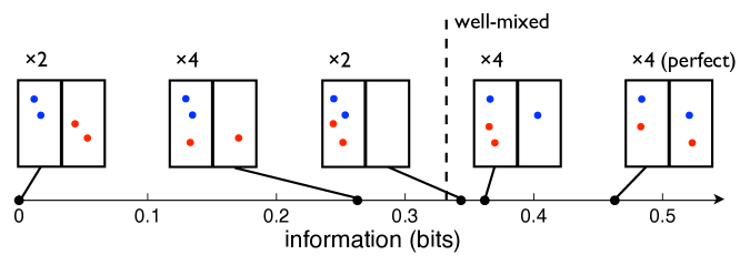
Figure 2B (dot-dashed curve) shows that the exchange of molecules between compartments increases the noise relative to the perfectly partitioned system considered previously when . This is because many of the alternative configurations generated by exchange lead to significant correlations between the states of the different molecules. Nevertheless, we see that the noise remains lower than that of the well-mixed system, because of the existence of some configurations in which the molecules are independent. However, the appearance of alternate configurations also affects the mean response (Fig. 2A); in particular, the appearance of configurations in which and molecules do not occupy the same partitions, and hence no signal can be propagated, means that the maximal output level is reduced. Given this simultaneous change in both the input-output function and the noise, it is not immediately clear whether signaling reliability is improved relative to the well-mixed system. Computing the mutual information, we see that the information transmitted by the system with exchange ( bits) is significantly lower than that for the well-mixed system ( bits), showing that the reduction of the output range compromises signal transmission to an extent which cannot be overcome by the corresponding reduction in noise.
The decrease in information transmission upon incorporating molecule exchange in the system with is the result of the appearance of suboptimal protein configurations, for which signal propagation is compromised (or even impossible). However, the number and performance of such configurations will in general depend on the relative values of , and (which need not equal or ). While molecule exchange may make partitioning unfavorable in the extreme case of , for systems with higher protein numbers it can be beneficial to partition the system into compartments, as we will see next.
1.5 An optimal partition size
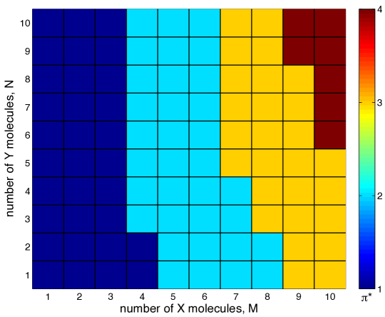
To study the performance of systems with higher protein numbers and different partition sizes, we compare the information transmission, including molecule exchange, for different partition numbers as the number of proteins in the system is varied while holding . Figure 5A shows that for protein copies, systems with partition do indeed outperform the well-mixed system. Furthermore, as is increased the optimal partition number also increases such that the optimal number of proteins per partition is roughly constant (Fig. 5B). This result is robust to variations in and : changing each over several orders of magnitude results in optimal partition sizes in the range (Appendix C: Fig. 9A and B). The assumption of is also not crucial for this result. In fact, we find that the value of has only a weak dependence on (Appendix C: Fig. 10).
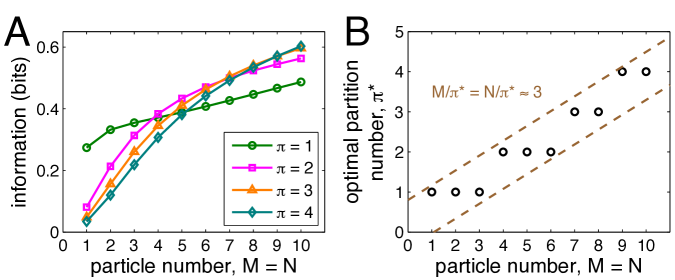
The optimal partition size arises from a trade-off between the reliability and efficiency of signaling. Increasing the number of partitions decreases the typical number of proteins per partition, which leads to the beneficial effects of a more graded response and reduced noise, increasing signaling reliability. On the other hand, due to molecule exchange, reducing the number of molecules per partition also increases the probability that any partition contains proteins of only one species that are therefore excluded from the signaling process, which leads to a reduced maximal response, reducing signaling efficiency.
The optimal size revealed by our study of molecules per species per partition shows good quantitative agreement with the observed aggregation of CD59 receptors ( molecules [7, 8]) and Ras proteins ( molecules [9, 10]), which each signal via the present motif and are known to interact with rafts and the cytoskelton. It is of further interest that a recent experiment in which T cell receptors were artificially partitioned on supported membranes found that the minimum number of agonist-bound receptors per partition necessary for downstream signaling is approximately four [20].
1.6 An explicitly spatial model
Lastly, we confirm that the effects observed in these minimal model systems, where the contents of each compartment are well-mixed and exchange can occur between any pair of compartments, persist in a more realistic model in which the diffusion of molecules in space is included explicitly. We simulate the diffusion and reaction of and molecules on a two-dimensional lattice, as described in Appendix A.3. The system is partitioned into a number of subdomains by the introduction of diffusion barriers, which are crossed with a reduced probability relative to regular diffusion steps on the lattice. Results of such simulations are shown in Fig. 6.
Figure 6A and B reveal that as the strength of the diffusion barriers is increased, the mean response becomes more graded, and the variance of activity is reduced, analogous to the two effects observed in the minimal model system (Fig. 2). When , one molecule of each species is permanently confined to a compartment, producing the graded response predicted for the perfectly partitioned system (Fig. 6A) and the associated minimal, binomial noise (Fig. 6B). Low but finite allows exchange of molecules between neighboring compartments but preserves a separation of timescales between intra- and inter-compartment mixing. This results in a graded mean response whose maximal level is reduced (Fig. 6A) and reduced noise (Fig. 6B), precisely the features observed in the minimal model of partitioning with exchange (Fig. 2). When , there are no barriers, and the system approaches the well-mixed limit (CME). Interestingly, however, the response remains more graded and the noise remains lower than the predictions of the CME due to the finite speed of diffusion (Fig. 6A and B), with agreement only reached when the ratio of diffusion to reaction propensities is much greater than one. This observation reveals that finite diffusion imposes an effective partitioning even when no actual partitions exist: molecules remain correlated with reaction partners within a typical distance set by diffusion, but uncorrelated with partners beyond this distance. As such, in the context of coupled reversible modification, we find that slower diffusion can linearize the response and reduce the noise, thereby improving information transmission.111Interestingly, this result is in marked contrast to the case of boundary establishment in embryonic development, where faster diffusion reduces noise within each nucleus by washing out bursts of gene expression in the input signal [21]. While in the present system faster diffusion will similarly reduce any super-Poissonian component of the noise within each partition individually, this averaging does not reduce the noise in the total output across all partitions. In fact, the latter noise is enhanced with faster diffusion by virtue of increased correlations between partitions. It is important to emphasize, however, that the extent of this effect is much smaller than for actual partitioning: Fig. 6B shows that finite diffusion reduces the maximal noise by , while strong partitioning () reduces the maximal noise by . Therefore, partitioning, which introduces not only a slower effective “hop” diffusion but also a separation of timescales between intra- and inter-compartmental mixing, is far more effective at conveying an information enhancement.
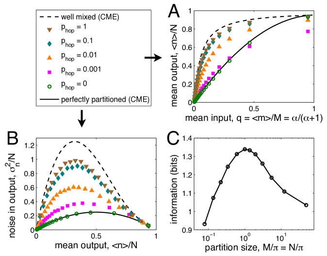
Fig. 6C confirms that the transmitted information varies non-monotonically with the number of barriers in a fixed area, indicating that an optimal partition size also appears in systems where space is modeled explicitly. Like in the minimal model, this optimum persists with changes in and , spanning the range of molecules per partition (Appendix C: Fig. 9C and D). Fig. 6C also provides a measure of the scale of information transmitted by this motif. In absolute terms, the optimal information ( bits) is consistent with values recently measured for signaling via the TNF-NF-B pathway ( bits) [22] and for patterning in the Drosophila embryo ( bits) [23]. In relative terms, we see that partitioning increases information over the unpartitioned system by (Fig. 6C) and decreases the maximal noise by (Fig. 6B). Thus, in both absolute and relative terms, we see that partitioning plays a critical role in producing informative and reliable membrane signaling.
As a final test, we use simulation to confirm that the effects of partitioning persist in the presence of features that are more realistic for signaling systems at the membrane, including extrinsic noise in the input (Appendix C: Fig. 11) and receptor dimerization (Appendix C: Fig. 12). The fact that the effects of partitioning, including the emergence of an optimal partition size, are robust to these details further underscores the generality of our findings.
2 Discussion
We have seen that the partitioning of a biochemical signaling system into a number of non-interacting subsystems improves the reliability of signaling via two effects. First, the non-linear response of the network means that a reduction in the number of input molecules translates into a more graded input-output response. Second, partitioning significantly reduces the noise in the response by eliminating correlations between the states of the different output molecules, an effect which, remarkably, overcomes the increase in noise associated with fewer input molecules in each subsystem. On the other hand, we have seen that the introduction of diffusion or exchange of molecules between partitions enhances the variance and reduces the range of the response, thereby reducing signaling performance. This result is due to the presence of configurations in which the two species are isolated from one another, compromising or even arresting signal transmission in certain partitions. The interplay between these two effects leads to a partition size that optimizes information transmission, corresponding to a few molecules per partition on average, in quantitative agreement with experiments. These effects are generic, and hence the emergence of an optimal partition size is robust to the specific parameters of the model. Notably, the underlying mechanism revealed here, namely the removal of correlations, differs fundamentally from that based on cooperativity in protein activation, which has been argued to underlie optimal cluster size in sensory systems [24, 25].
Reversible modification reactions are ubiquitous in cell signaling, and interactions with the cytoskeleton and lipids provide general mechanisms for the formation of subdomains. We therefore expect the results revealed by our study to be applicable to a wide class of signaling systems at the membrane. We have focused in this paper on coupled single-site modification reactions because this motif governs pathways specifically known to be affected by the formation of membrane sub-domains. However, the effects we uncover also pertain to multi-site modification reactions, which are very common in cell signaling [26, 27, 28, 29]. Moreover, we have focused on systems where the reactant species are confined by a boundary which limits diffusion. However, similar effects could be observed in systems where proteins are localized to raft domains, or even scaffolds or large macromolecular complexes. In the latter case, each complex would effectively provide an independent reaction “compartment,” and the exchange between compartments would be the result of rare dissociation events, after which proteins could diffuse rapidly through the cytoplasm to a different complex. Even if the signal within each complex was not mediated via diffusive encounters, but rather via cooperative or allosteric interactions, the fundamental mechanism that we reveal here – that partitioning into subsystems removes correlations between subsystems – remains at play. The presence of scaffolds and macromolecular complexes at early stages of signaling pathways is extremely common [30], suggesting that the effects discussed here are of wide biological relevance.
3 Methods
The CME (1) is solved using the method of spectral expansion [15, 16]. Details of this method, the computation of mutual information, and the spatial simulations are described in Appendix A. Source code, written in MATLAB, C++, and Mathematica, used to generate all results and figures in the main text and the SI Appendix is freely available at http://partitioning.sourceforge.net.
4 Acknowledgments
This work is part of the research program of the “Stichting voor Fundamenteel Onderzoek der Materie (FOM)”, which is financially supported by the “Nederlandse organisatie voor Wetenschappelijk Onderzoek (NWO)”. We thank Philippe Nghe for a critical reading of the manuscript.
Appendix A Detailed methods
A.1 Spectral solution of the master equation
The chemical master equation (CME) is solved using the method of spectral expansion [15, 16], described in detail in Appendix B. Briefly, the structure of of the CME, in which the dynamics can be separated into two operators that act only on or but not both, allows for its solution to be written in the form , where is the eigenvector of the operator and similarly for , and is an expansion parameter on which does not ultimately depend. The expansion coefficients can be calculated straightforwardly, as shown in Appendix B. Importantly, this spectral expansion dramatically decreases the computational complexity of calculating : rather than solving the system of the original CME, it is only necessary to solve linear systems of size for the vectors of coefficients . We emphasize that since the system has a finite state-space, no approximations are made in using the spectral expansion, and the solution remains exact. Furthermore, the moments of the steady-state distribution can be conveniently expressed in terms of the expansion coefficients ; in particular, and .
A.2 Mutual information
The mutual information between network input and response is given by the standard expression [18] , where the average is taken over the joint distribution , and is given by the steady state of the CME. The calculation of the mutual information requires specification of the distribution of input signals . We choose values of such that is uniformly-spaced over the range ; then and . However, our conclusions are unaffected if we instead take a input distribution that is unimodal or bimodal (Fig. 13). We take , for which converges to within of its large- limit (Fig. 14).
A.3 Spatial simulations
The diffusion and reactions of molecules and molecules are simulated on a two-dimensional square lattice of side length using a fixed-time-step integration scheme. During each step of duration , each particle is moved to a random neighboring lattice site with probability , where is the diffusion constant, and is the lattice spacing. Molecules have steric interactions on the lattice, such that only one molecule can be present at each lattice site at any time. Attempted moves to an occupied site are rejected, with the particle remaining at its original position. If a molecule in the state is adjacent to a molecule in the state, the latter is converted to the state with probability . To make partitions, linear diffusion barriers are placed at in each direction, where . A diffusion step which crosses such a barrier is accepted with probability reduced by a factor . The time step is chosen sufficiently small that no probability exceeds one.
Appendix B Solution of the master equation by spectral expansion
This section describes the solution via the method of spectral expansion, or the ‘spectral method’, of the CME introduced in the main text. The spectral method has been used fruitfully in the context of gene regulation to solve CMEs describing cascades [15], bursts [16], and oscillations [31], and a pedagogical treatment is available in [32]. Here we apply the spectral method to coupled reversible switching.
From Eqns. 1-2 of the main text, the stochastic dynamics of the system under study are given by the CME
| (7) |
where both operators and have the form
| (8) |
with defining the step operator. The CME describes the evolution of the probability of having proteins in the active state and proteins in the active state, with the coupling function by which drives the activation of .
B.1 The moments do not close
We first demonstrate that direct computation of the moments from the CME is not possible because the moments do not close. The reason is that a nonlinearity is present in the first term of Eqn. 8 in the form of the factor . As a result, the first moment depends on a higher moment, which in turn depends on an even higher moment, and so on.
To see explicitly that the moments do not close, we consider computing the dynamics of the first moment of the driven species, the mean , by summing the CME over and against . We obtain
| (9) |
where averages are taken over . We see that indeed the final term carries the nonlinearity. Even for the simplest coupling function, i.e. linear coupling , one finds a hierarchy of moment dependencies that does not close:
| (10) | |||||
| (11) | |||||
| (12) |
That is, the dynamics of depend on , whose dynamics depend on , and so on.
The fact that the moments cannot be computed—indeed, not even the mean output —makes it particularly important to actually solve the CME in order to learn about the statistical properties of this system.
B.2 The spectrum of the switch operator
The CME is a linear equation. Even when the rates are nonlinear functions of the molecule numbers, the CME is still linear in its degree of freedom, the joint probability. The most straightforward way to solve a linear equation is to write its solution as an expansion in the eigenfunctions of the linear operator. Although it is difficult to derive the eigenfunctions of the coupled operator , it is straightforward to derive the eigenfunctions of the uncoupled operator , which we call the switch operator. Indeed, we will see that expanding the joint probability in eigenfunctions of the uncoupled operator greatly simplifies the form of the CME, yielding an exact solution in terms of matrix algebra.
The switch operator governs the CME for the first species ; explicitly,
| (13) |
where for notational simplicity we have taken . Its eigenvalue relation is written
| (14) |
for eigenvalues and eigenvectors .
B.2.1 Eigenvalues
The matrix form of the operator can be read directly from Eqn. 13:
| (15) |
The tridiagonal structure follows from the fact that molecule numbers only increase or decrease by one at a time. Practically speaking, the eigenvalues can be obtained using the fact that the determinant of a tridiagonal matrix can be computed recursively. Performing the computation for reveals the pattern
| (16) |
However, Eqn. 16 can be derived more rigorously by making use of a generating function. We present this derivation next, since the generating function formalism will also prove quite useful in deriving the eigenvectors and solving the CME.
The generating function is an expansion in any complete basis for which the probability distribution provides the expansion coefficients [33]. Choosing as our basis the set of polynomials in some continuous variable , the generating function is defined
| (17) |
The probability distribution is recovered via the inverse transform
| (18) |
A key utility of the generating function is turning the CME, which is a set of ordinary differential equations (ODEs), into a single partial differential equation. Indeed, summing Eqn. 13 against yields
| (19) |
where the appearances of and arise from the shifts and , respectively. Eqn. 19 directly gives the form of the operator in space: . The eigenfunctions are then obtained from the relation by separating variables and integrating:
| (20) |
Here, the constant factor is determined by application of the normalization condition to the steady state solution, which is obtained by setting :
| (21) |
We will solve Eqn. 19 in two ways: by the method of characteristics and by expansion in the eigenfunctions; together these solutions will reveal the eigenvalues.
First, the method of characteristics [34] posits that the dependence of on and occurs via some parametric variable , i.e. . The chain rule then gives , which when compared term by term with Eqn. 19 yields three ordinary differential equations:
| (22) |
The first identifies , with which the second is solved by
| (23) |
where is a constant of integration. The crux of the method is that Eqn. 23 defines a characteristic curve on which must depend, i.e. , where and are unknown functions, and has been promoted to a characteristic function of and . The function is identified by realizing that steady state is reached as , for which no longer depends on or . Therefore, must be the steady state function given in Eqn. 21:
| (24) |
Although we still do not know , we may Taylor expand it around the point , yielding
| (25) |
where .
Second, because Eqn. 19 is linear, we may also write down its solution as an expansion in the eigenfunctions of its linear operator:
| (26) |
Under the assumption that the eigenfunctions are orthogonal (which will be shown in the next section), inserting Eqn. 26 into Eqn. 19 yields an independent ODE for each , , which is solved by for initial conditions . Inserting this functional form and that for (Eqn. 20) into Eqn. 26 yields
| (27) |
Comparison of Eqns. 25 and 27 reveals both the expression for the eigenvalues, , and a limit on their domain, the nonnegative integers . Of course, the domain can be a subset of the nonnegative integers; then some in Eqn. 27 would be zero. Indeed, since is a finite matrix of size by (Eqn. 15), it is spanned by linearly independent eigenvectors, meaning we expect only eigenvalues. In fact, the only set of nonnegative integers that satisfies the requirement that the trace of , , equals the sum of the eigenvalues, , is . Thus, we arrive at the result
| (28) |
as proposed by inspection in Eqn. 16.
B.2.2 State space notation
The linear algebraic manipulations we have done thus far can be cast in the more abstract notation of state spaces, commonly used in quantum mechanics [35]. We will find this notation useful in later sections, for example in transforming between the molecule number basis and the eigenbasis. Specifically, we introduce a state that can be projected into space to give the probability distribution, or into space to give the generating function:
| (29) |
In the same way, the th eigenstate is projected into space to give the th eigenvector, or into space to give the th eigenfunction:
| (30) |
This notation offers new insight into our definition of the generating function. For example, Eqn. 17 can now be written
| (31) |
where we have recognized
| (32) |
as the projection of the state into space. Eqn. 31 has a clear interpretation: we have inserted a complete set of states. Similarly, Eqn. 18 can now be written
| (33) |
In the first step, we have rewritten Eqn. 18 using Cauchy’s theorem, where , and the contour surrounds the pole at . In the second step, we have recognized
| (34) |
as the conjugate to . Eqn. 33 has the clear interpretation of inserting a complete set of states, under an inner product defined by the complex integration. The choice of inner product and of conjugate state are made such that orthonormality is preserved, a fact which we may confirm by again employing Cauchy’s theorem:
| (35) |
Finally, the dynamics in Eqn. 19 can be written in state space as
| (36) |
where we have defined the operators and whose projections in space are and . These are analogous to the raising and lowering operators in the well known treatment of the quantum harmonic oscillator. This operator formalism for the generating function was first developed in the 1970s; for a review see [36].
B.2.3 Eigenvectors
The state space notation facilitates a derivation of the functional form of the eigenvectors:
| (37) |
Here we have inserted the eigenfunctions
| (38) |
from Eqn. 20, with eigenvalues given by Eqn. 28. We use Cauchy’s theorem to perform the integration and recognize that derivatives of a product follow a binomial expansion:
| (39) | |||||
| (40) | |||||
| (41) | |||||
| (42) |
Here the domain results from the derivatives and is defined by . Eqn. 42 gives the expression for the eigenvectors. For the expression reduces to the binomial distribution in terms of the occupancy , as it must, since this is the steady state of the uncoupled process:
| (43) |
This function has one maximum, and in general the th eigenvector has extrema, making the eigenvectors qualitatively similar to Fourier modes or eigenfunctions of the quantum harmonic oscillator.
The switch operator is not Hermitian. A consequence is that its conjugate eigenvectors (row vectors) are not complex conjugates of its eigenvectors (column vectors). Rather, they are distinct functions that must be constructed to obey an orthonormality relation in order to constitute a complete basis. The orthonormality relation can be used to derive their form in space, :
| (44) |
Here we have defined and in order to draw an equivalence between Eqn. 44 and Eqn. 35, which then implies , or
| (45) |
Eqn. 45 gives the form of the conjugate eigenfunctions in space, which can be used to derive the expression for the conjugate eigenvectors as in Eqns. 37-42:
| (46) | |||||
| (47) |
Here is defined by . Eqn. 47 gives the expression for the conjugate eigenvectors. They are th order polynomials in .
B.3 Expanding the coupled problem in uncoupled eigenfunctions
We now solve the CME by expanding the solution in the eigenfunctions of the uncoupled operator. This procedure is most easily done in state space, in which the CME reads
| (48) |
where
| (49) | |||||
| (50) |
as in Eqn. 36, and we have introduced the operator whose action on the state yields the coupling function, . The first step is to write the full operator as two uncoupled operators plus a correction term. Introducing the constant to parameterize the second uncoupled operator, the CME becomes
| (51) |
where we have explicitly denoted the fact that the correction term factorizes into two operators that act on each of the and sectors alone:
| (52) | |||||
| (53) |
The second step is to expand the solution in the eigenfunctions of the two uncoupled operators. Introducing as the mode index for the eigenstates of , we write
| (54) |
Inserting this form into the CME, projecting with the conjugate state , and summing over and yields the dynamics for the expansion coefficients :
| (55) |
Here the first term is diagonal and reflects the actions of the uncoupled operators on their eigenstates. The second term contains the corrections and . The first correction is directly evaluated by inserting a complete set of states:
| (56) | |||||
| (57) |
We see that is the simply the difference between the coupling function and the constant parameter, rotated into eigenspace. Notably, for linear coupling, is tridiagonal (see Sec. B.5). The second correction is most easily evaluated by inserting a complete set of states; the result, derived in Sec. B.5, is
| (58) |
We see that is subdiagonal in , which simplifies the dynamics of to
| (59) |
where we define the matrix acting on the diagonal part as
| (60) |
The subdiagonality allows one to write the steady state of Eqn. 59 as an iterative scheme, by which the th column of is computed from the th column:
| (61) |
The scheme is initialized with
| (62) |
(see Sec. B.5), and the joint distribution is recovered via
| (63) |
which is the projection of Eqn. 54 into space.
Eqn. 63 constitutes an exact steady state solution to the CME, with computed iteratively via Eqns. 61 and 62, auxiliary matrices defined in Eqns. 57 and 60, and the eigenvectors given by Eqns. 42 and 47. Importantly, the computational complexity of the solution has been dramatically reduced: rather than solving the original CME (Eqn. 7), which requires inverting its operator of size , Eqn. 61 makes clear that it is only necessary to invert smaller matrices of size , i.e. the matrices for .
B.4 Exact expressions for moments
Now that we have an exact solution to the CME in terms of a spectral expansion, moments take an exact form in terms of the expansion coefficients. We thus circumvent the problem of moment closure, instead arriving at compact expressions that require only the inversion and multiplication of finite matrices via Eqn. 61.
Moments are most easily computed from the generating function, . For example, the th moment of the output is
| (64) |
In terms of the expansion, the generating function is , and using the fact that (Eqn. 38), we have
| (65) |
Inserting the expression for (Eqn. 38) and defining , we obtain
| (66) |
At this point we recall that is a constant we introduce to parameterize the expansion. The expression for the moments therefore cannot depend on : if we change , the expression in brackets changes, but the expansion coefficients also change, such that Eqn. 66 evaluates to the same -independent form. We are therefore free to set to any value, and the choice makes the derivative easiest to evaluate. Thus we have
| (67) |
where it is now understood that is computed with . Evaluating the derivative yields
| (68) | |||||
| (69) | |||||
| (70) |
in terms of the Stirling numbers of the second kind,
| (71) |
For example, the first moment, second moment, and variance are
| (72) | |||||
| (73) | |||||
| (74) |
These are exact expressions for the moments in terms of the expansion coefficients , which are obtained by matrix inversion and multiplication via Eqn. 61, e.g. in Mathematica.
An informative special case is immediately revealed when , for which does not exist, i.e. and , or
| (75) |
Here there is only one output molecule. The relationship between its mean activation and the associated noise must therefore obey the known result for a single binary switch, Eqn. 75.
B.5 Auxiliary calculations
Here we show that is tridiagonal for linear :
| (76) | |||||
| (77) | |||||
| (78) | |||||
| (79) | |||||
| (81) | |||||
| (84) | |||||
| (85) | |||||
| (86) | |||||
| (87) |
Eqn. 77 recognizes that is the operator representation of (since is the number operator, i.e. ), and Eqn. 84 uses the algebraic fact that , which is straightforward to verify.
Here we derive Eqn. 58:
| (88) | |||||
| (89) | |||||
| (90) | |||||
| (91) | |||||
| (94) | |||||
| (95) | |||||
| (96) | |||||
| (97) | |||||
| (98) | |||||
| (99) | |||||
| (100) |
Appendix C Supplementary figures
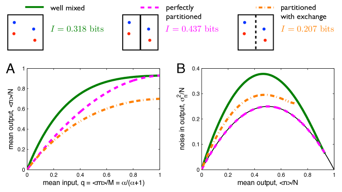
A, B As in Fig. 2 of the main text, with , perfect partitioning linearizes the input-output relation and reduces the noise, transmitting more information than the well-mixed system; further, allowing exchange among partitions compresses the response and increases the noise compared to the perfectly partitioned system, transmitting less information than the well-mixed system.
C, D As in Fig. 5 of the main text, an information-optimal partition size, here , emerges due to the trade-off between optimizing signaling reliability and avoiding unfavorable configurations.
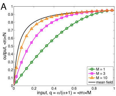
A The output (the mean activity of molecules) vs. the input (the mean activity of molecules) for several values of . As is reduced the response becomes more linear, deviating more strongly from the mean-field response . Symbols show uniformly spaced values of to highlight the effect of saturation on the state space.
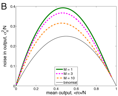
B The noise vs. the mean for the output, shown for the same values of . As is reduced the noise increases for all values of the mean.
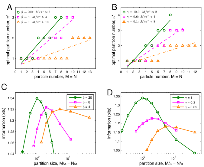
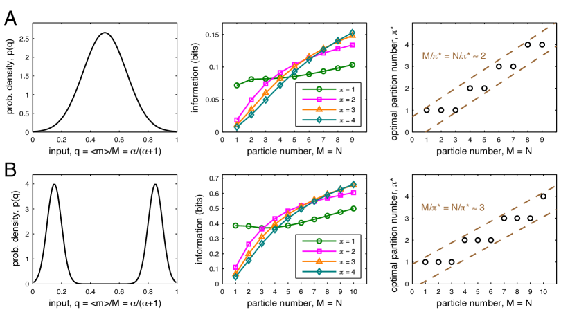
A, B Results from the minimal system, described by the chemical master equation, as in Fig. 5B of the main text. The information-optimal partition number is plotted as a function of molecule number for various values of (A) and (B). Linear fits provide estimates of the optimal partition size , as indicated in the legends. In A, ; in B, .
C, D Results from the lattice simulation, in which space is accounted for explicitly, as in Fig. 6C of the main text. The information is plotted as a function of the partition size, directly revealing an optimum, for various values of (C) and (D). Parameters are as in Fig. 6C: , , , and . In C, ; in D, .
As discussed in the main text, the optimum arises due to a tradeoff between two key effects of partitioning: on the one hand, partitioning removes correlations in the states of molecules, reducing noise; on the other hand, partitioning isolates molecules, reducing the maximal response. The first effect favors few molecules per partition, while the second effect favors many molecules per partition.
As seen here in both the minimal system (A, B) and the simulated system (C, D), lowering or increases the optimal number of molecules per partition. This result has an intuitive explanation in terms of the above tradeoff: lowering either or slows the rate of switching from the to the state, with respect to the timescale of switching. As a result, molecules are less sensitive to individual fluctuations in the state of molecules. The states of the molecules therefore exhibit weaker correlations, which in turn weakens the benefit that partitioning imparts in terms of the removal of these correlations. The opposing effect of molecular isolation thus begins to dominate, pushing the optimum toward a larger number of molecules per partition.
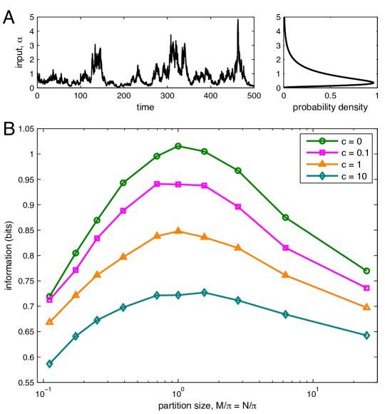
A Simulations are performed with extrinsic noise introduced to the input parameter . To keep , the quantity is described by the simple mean-reverting Ornstein-Uhlenbeck process , where is a Gaussian random variable with mean and variance ; this results in a log-normal distribution for . The quantity is the autocorrelation time, and the choices and ensure that the mean of is and that the variance of scales with the mean via .
B As the magnitude of the extrinsic noise (set by ) increases, the information decreases for all partition sizes, while the presence of an information-optimal partition size persists.
Here , , , , the system is lattice spacings squared, the ratio of diffusion to reaction propensities is , and in units of the reaction rate (which sets the timescale of switching). In A, and time is scaled by . In B, when , the information transmission is lower than that in Fig. 6C of the main text because is lower.
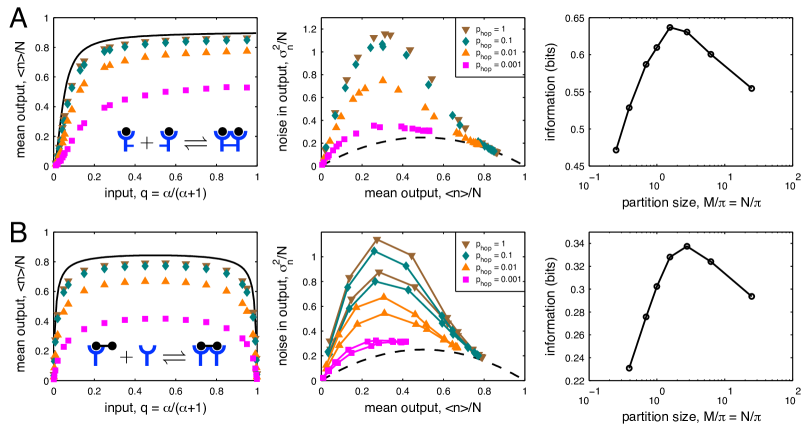
Left As in Fig. 6A of the main text, as the probability of crossing a diffusion barrier is decreased, the maximal value of the mean response decreases. In A, the response also becomes more linear, but to less of a degree than in Fig. 6A of the main text. Note that due to both finite diffusion and finite molecule number, even the unpartitioned response () deviates from the mean-field response (black solid line), which is given by , where is the fraction of molecules in the dimer state; in A, with , while in B, with . Here . Legends in middle panels apply to left panels as well.
Middle As in Fig. 6B of the main text, as the probability of crossing a diffusion barrier is decreased, the output noise decreases. Black dashed line shows the binomial noise limit . In B, lines connecting data points are provided to reveal that, as there are two values of that give the same mean (left), the noise is higher for the smaller value of . Here .
Right As in Fig. 6C of the main text, the tradeoff between reliable signaling (reduced noise) and efficient signaling (maintaining a high maximal response) leads to an information-optimal partition size. Here . Here, the information transmission is lower than that in Fig. 6C of the main text because is lower and additionally, in B, because of the non-monotonic mean response.
References
- [1] Hernán E Grecco, Malte Schmick, and Philippe I H Bastiaens. Signaling from the living plasma membrane. Cell, 144(6):897–909, Mar 2011.
- [2] Christian Eggeling, Christian Ringemann, Rebecca Medda, Günter Schwarzmann, Konrad Sandhoff, Svetlana Polyakova, Vladimir N Belov, Birka Hein, Claas von Middendorff, Andreas Schönle, and Stefan W Hell. Direct observation of the nanoscale dynamics of membrane lipids in a living cell. Nature, 457(7233):1159–62, Feb 2009.
- [3] Daniel Lingwood and Kai Simons. Lipid rafts as a membrane-organizing principle. Science, 327(5961):46–50, Jan 2010.
- [4] A Kusumi and Y Sako. Cell surface organization by the membrane skeleton. Current Opinion in Cell Biology, 8(4):566–74, Aug 1996.
- [5] Akihiro Kusumi, Yuki M Shirai, Ikuko Koyama-Honda, Kenichi G N Suzuki, and Takahiro K Fujiwara. Hierarchical organization of the plasma membrane: investigations by single-molecule tracking vs. fluorescence correlation spectroscopy. FEBS Letters, 584(9):1814–23, May 2010.
- [6] Boris N Kholodenko, John F Hancock, and Walter Kolch. Signalling ballet in space and time. Nat Rev Mol Cell Biol, 11(6):414–26, Jun 2010.
- [7] Kenichi G N Suzuki, Takahiro K Fujiwara, Fumiyuki Sanematsu, Ryota Iino, Michael Edidin, and Akihiro Kusumi. GPI-anchored receptor clusters transiently recruit Lyn and G alpha for temporary cluster immobilization and Lyn activation: single-molecule tracking study 1. The Journal of Cell Biology, 177(4):717–30, May 2007.
- [8] Kenichi G N Suzuki, Takahiro K Fujiwara, Michael Edidin, and Akihiro Kusumi. Dynamic recruitment of phospholipase C gamma at transiently immobilized GPI-anchored receptor clusters induces IP3-Ca2+ signaling: single-molecule tracking study 2. The Journal of Cell Biology, 177(4):731–42, May 2007.
- [9] Ian A Prior, Cornelia Muncke, Robert G Parton, and John F Hancock. Direct visualization of Ras proteins in spatially distinct cell surface microdomains. The Journal of Cell Biology, 160(2):165–70, Jan 2003.
- [10] S. Plowman, C. Muncke, R. G. Parton, and J. F. Hancock. H-ras, K-ras, and inner plasma membrane raft proteins operate in nanoclusters with differential dependence on the actin cytoskeleton. Proc. Natl Acad. Sci. USA, 102:15500–15005, 2005.
- [11] Ziya Kalay, Takahiro K Fujiwara, and Akihiro Kusumi. Confining domains lead to reaction bursts: reaction kinetics in the plasma membrane. PLoS ONE, 7(3):e32948, Jan 2012.
- [12] Andrew Mugler, Aimee Gotway Bailey, Koichi Takahashi, and Pieter Rein ten Wolde. Membrane clustering and the role of rebinding in biochemical signaling. Biophysical Journal, 102(5):1069–78, Mar 2012.
- [13] T. Tian, A. Harding, K. Inder, S. Plowman, R. G. Parton, and J. F. Hancock. Plasma membrane nanoswitches generate high-fidelity Ras signal transduction. Nat. Cell Biol., 9:905–914, 2007.
- [14] Thomas Gurry, Ozan Kahramanoğullari, and Robert G Endres. Biophysical mechanism for Ras-nanocluster formation and signaling in plasma membrane. PLoS ONE, 4(7):e6148, Jan 2009.
- [15] A M Walczak, A Mugler, and C H Wiggins. A stochastic spectral analysis of transcriptional regulatory cascades. Proc Natl Acad Sci USA, 106:6529–6534, 2009.
- [16] A Mugler, A M Walczak, and C H Wiggins. Spectral solutions to stochastic models of gene expression with bursts and regulation. Phys Rev E, 80:041921, 2009.
- [17] J. L. W. V. Jensen. Sur les fonctions convexes et les inégalités entre les valeurs moyennes. Acta Mathematica, 30(1):175–193, 1906.
- [18] C. E. Shannon. A Mathematical Theory of Communication. Bell Syst Tech J, 27:379–423, 623–656, 1948.
- [19] Kotono Murase, Takahiro Fujiwara, Yasuhiro Umemura, Kenichi Suzuki, Ryota Iino, Hidetoshi Yamashita, Mihoko Saito, Hideji Murakoshi, Ken Ritchie, and Akihiro Kusumi. Ultrafine membrane compartments for molecular diffusion as revealed by single molecule techniques. Biophysical Journal, 86(6):4075–93, Jun 2004.
- [20] Boryana N Manz, Bryan L Jackson, Rebecca S Petit, Michael L Dustin, and Jay Groves. T-cell triggering thresholds are modulated by the number of antigen within individual T-cell receptor clusters. Proc Natl Acad Sci USA, 108(22):9089–94, May 2011.
- [21] Thorsten Erdmann, Martin Howard, and Pieter Rein ten Wolde. Role of spatial averaging in the precision of gene expression patterns. Phys. Rev. Lett., 103:258101, Dec 2009.
- [22] Raymond Cheong, Alex Rhee, Chiaochun Joanne Wang, Ilya Nemenman, and Andre Levchenko. Information transduction capacity of noisy biochemical signaling networks. Science, 334(6054):354–8, Oct 2011.
- [23] Gasper Tkacik, Curtis G Callan, and William Bialek. Information flow and optimization in transcriptional regulation. Proceedings of the National Academy of Sciences, 105(34):12265–70, Aug 2008.
- [24] Gerardo Aquino, Diana Clausznitzer, Sylvain Tollis, and Robert G Endres. Optimal receptor-cluster size determined by intrinsic and extrinsic noise. Physical Review E, 83:21914, Feb 2011.
- [25] Monica Skoge, Yigal Meir, and Ned S Wingreen. Dynamics of cooperativity in chemical sensing among cell-surface receptors. Physical Review Letters, 107:178101, Oct 2011.
- [26] Koichi Takahashi, Sorin Tanase-Nicola, and Pieter Rein ten Wolde. Spatio-temporal correlations can drastically change the response of a MAPK pathway. Proc Natl Acad Sci USA, 107(6):2473–8, Feb 2010.
- [27] Jeroen S van Zon, David K Lubensky, Pim R H Altena, and Pieter Rein ten Wolde. An allosteric model of circadian KaiC phosphorylation. Proc Natl Acad Sci USA, 104(18):7420–5, May 2007.
- [28] Paul Miller, Anatol M Zhabotinsky, John E Lisman, and Xiao-Jing Wang. The stability of a stochastic CaMKII switch: dependence on the number of enzyme molecules and protein turnover. Plos Biol, 3(4):e107, Apr 2005.
- [29] P Nash, X Tang, S Orlicky, Q Chen, F B Gertler, M D Mendenhall, F Sicheri, T Pawson, and M Tyers. Multisite phosphorylation of a CDK inhibitor sets a threshold for the onset of DNA replication. Nature, 414(6863):514–21, Nov 2001.
- [30] A. Zeke, M. Lukács, W. A. Lim, and A. Reményi. Scaffolds: interaction platforms for cellular signalling circuits. Trends Cell Biol., 19:364–374, 2009.
- [31] A Mugler, A M Walczak, and C H Wiggins. Information-optimal transcriptional response to oscillatory driving. Phys Rev Lett, 105:058101, 2010.
- [32] A M Walczak, A Mugler, and C H Wiggins. Analytic methods for modeling stochastic regulatory networks. In X Liu and M Betterton, editors, Methods in Molecular Biology, Vol. 880: Computational Modeling of Signaling Networks. Humana Press, 2012.
- [33] N G van Kampen. Stochastic processes in physics and chemistry. Elsevier Science, 2nd edition, 1992.
- [34] S J Farlow. Partial differential equations for scientists and engineers. Dover Publications, 1993.
- [35] J S Townsend. A modern approach to quantum mechanics. University Science Books, 2000.
- [36] D C Mattis and M L Glasser. The uses of quantum field theory in diffusion-limited reactions. Rev Mod Phys, 70:979–1001, 1998.
- [37] M A Lemmon and J Schlessinger. Cell signaling by receptor tyrosine kinases. Cell, 141:1117–34, 2010.
- [38] S Schlee, P Carmillo, and A Whitty. Quantitative analysis of the activation mechanism of the multicomponent growth-factor receptor Ret. Nat Chem Biol, 2:636–44, 2006.