Why multi-tracer surveys beat cosmic variance

Abstract

Galaxy surveys that map multiple species of tracers of large-scale structure can improve the constraints on some cosmological parameters far beyond the limits imposed by a simplistic interpretation of cosmic variance. This enhancement derives from comparing the relative clustering between different tracers of large-scale structure. We present a simple but fully generic expression for the Fisher information matrix of surveys with any (discrete) number of tracers, and show that the enhancement of the constraints on bias-sensitive parameters are a straightforward consequence of this multi-tracer Fisher matrix. In fact, the relative clustering amplitudes between tracers are eigenvectors of this multi-tracer Fisher matrix. The diagonalized multi-tracer Fisher matrix clearly shows that while the effective volume is bounded by the physical volume of the survey, the relational information between species is unbounded. As an application, we study the expected enhancements in the constraints of realistic surveys that aim at mapping several different types of tracers of large-scale structure. The gain obtained by combining multiple tracers is highest at low redshifts, and in one particular scenario we analyzed, the enhancement can be as large as a factor of $\gtrsim 3$ for the accuracy in the determination of the redshift distortion parameter, and a factor $\gtrsim 5$ for the local non-Gaussianity parameter $f_{NL}$. Radial and angular distance determinations from the baryonic features in the power spectrum may also benefit from the multi-tracer approach.

1 Introduction

Recent advances in Cosmology, in particular those related to the present epoch of accelerated expansion, have been overwhelmingly driven by astrophysical surveys (York et al., 2000; Cole et al., 2005; Abbott et al., 2005; Scoville et al., 2007; Adelman-McCarthy et al., 2008a, b; PAN-STARRS, ; BOSS, ; Blake et al., 2011). The legacies of these surveys are a set of increasingly tight constraints on cosmological parameters and powerful tests of the robustness of the standard cosmological model, but also an alarming confirmation that there are gaping holes in that model.

The landscape of available instruments and observations is rapidly evolving. Besides general-purpose efforts that push the limits of what was achieved by the Sloan Digital Sky Survey (York et al., 2000) both in wavelength and in redshift (BigBOSS, ; SUMIRE, ; Ellis et al., 2012), now cosmologists can also count on surveys with a cadence aimed at discovering variable objects (Rau, 2009; Abell et al., 2009), and mapping large volumes of the universe with high completeness. The latter is achieved by imaging large areas of the sky with narrow-band filters (Benítez et al., 2009) or resorting to low-resolution (spectral as well as spatial) integral-field spectroscopy (Hill, 2008).

Galaxy redshift surveys are now expected to perform high-accuracy measurements of the equation of state of dark energy, test for models of modified gravity through lensing or redshift-space distortions (Linder, 2005), impose constraints on the amplitude of non-Gaussian features in the power spectrum (Verde et al., 2000; Bartolo et al., 2004), measure neutrino masses, etc. – see, e.g. (Benítez et al., 2009; SUMIRE, ; Ellis et al., 2012). Since many surveys are already reaching large fractions of the sky with high completeness, the variance due to the survey’s finite volume (i.e. cosmic variance) is perhaps the most formidable obstacle to further progress.

Interestingly, it has been pointed out by Seljak (2009); McDonald & Seljak (2008) that cosmic variance can be somehow circumvented for some cosmological parameters – see also Gil-Marín et al. (2010); Cai & Bernstein (2011a); Hamaus et al. (2011, 2012) . This is true, in particular, for the redshift-space distortion (RSD) parameter, $\beta(z)=f(z)/b(z)$, and for the amplitude of local non-Gaussianities, $f_{NL}$. The reason behind this “miracle” is that bias-sensitive parameters such as $\beta$ and $f_{NL}$ are not subject to the same random processes that lead to different realizations of the density field for some matter power spectrum $P(k)$. Therefore, given a fixed density field, by comparing the clusterings between different types of tracers of large-scale structure (i.e. objects which correspond to halos of different masses) we should be able to measure these parameters with a precision that is not limited by cosmic variance. We should point out that the source of this extra information is not some sub-Poissonian shot noise that can be achieved by, for example, mass-weighting instead of bias-weighting (Seljak et al., 2009; Cai et al., 2011), but is rather a direct consequence of the different relative amplitudes of the clustering among the tracers.

Using these ideas, Hamaus et al. (2011, 2012), constructed a covariance matrix for the ratios of the clusterings of any two types of tracers, and used N-body simulations to obtain enhanced constraints for $\beta$ and $f_{NL}$. Conversely, Slosar (2009) constructed the Fisher information for $f_{NL}$ directly from the covariance matrix for counts in cells under simplifying assumptions similar to ours. Gil-Marín et al. (2010), on the other hand, studied how non-linear bias and bias stochasticity can degrade the two-tracer constraints, and found that the actual improvements in the constraints may be up to $\sim$ 50% smaller, compared with the ideal case of linear and deterministic bias. Cai & Bernstein (2011a) pointed out that bias modulations between dark matter halos imply correlations between the biases of the tracers, which limits the potential gains of the multi-tracer approach. Cai & Bernstein (2011b) then analyzed how weak gravitational lensing tomography surveys can be combined with redshift surveys in order to mitigate those correlations, and to break the degeneracies between the biases and the other cosmological parameters of interest.

In this paper we show that the enhanced constraints of bias-sensitive parameters in multi-tracer surveys are a direct consequence of the Fisher matrix for multiple tracers of large-scale structure. The analysis is an extension of the single-tracer Fisher matrix of Feldman et al. (1994) (henceforth FKP) to multiple tracers of large-scale structure. What emerges from the multi-tracer Fisher matrix is, besides the usual cosmic variance-limited “effective volume” (Tegmark, 1997; Tegmark et al., 1998), simple expressions which quantify the amount of information that lies in the “relational" degrees of freedom, which are completely independent of the effective volume.

We show that there is a simple choice of variables which diagonalizes the multi-tracer Fisher matrix. The total effective volume of the survey then appears naturally as one of the terms of this diagonal matrix, while the remaining terms correspond to the information in the relative clusterings between the different species of tracers. The key aspect is that the Fisher matrix elements corresponding to the relational degrees of freedom are unbounded, and can in fact carry much more information about some parameters than the effective volume – which is, of course, bounded by the physical volume of the survey.

This paper is organized as follows: in Sec. 2 we review the statistics of galaxy surveys, and present the generalization of the FKP method to multiple tracers; in Sec. 3 we show how a certain choice of relative clusterings between the tracers leads to the diagonalization of the multi-tracer Fisher matrix; in Sec. 4 we show an application to a hypothetical survey of three types of tracers, and how the relational information improves the constraints; our conclusions comprise Sec. 5.

2 The statistics of galaxy surveys

The main observables galaxy surveys try to measure are the redshift-space matter power spectrum and its sub-products, such as the baryon acoustic oscillations (Eisenstein et al., 1999; Blake & Glazebrook, 2003; Seo & Eisenstein, 2003) and redshift-space distortions (Hamilton, 2005a, b). In terms of the matter density contrast $\delta(\vec{x})$, the position-space power spectrum is given by the expectation value $\langle\delta(\vec{k},z)\delta^{*}(\vec{k}^{\prime},z)\rangle=(2\pi)^{3}P(k,z)\delta_{D}(\vec{k}-\vec{k}^{\prime})$, where $\delta_{D}$ is the Dirac delta function.

The problem with this program is that we cannot directly measure the fluctuations of the matter field in position space. Instead, what we observe are counts of tracers of the large-scale structure in redshift space. In the simplest approximation, bias and redshift distortions can be regarded as operators acting on the density contrast, such that the fluctuation field of some tracer $\alpha$ (where $\alpha$ stands for galaxies of a certain type) in redshift space is related to the underlying mass fluctuation field in position space by some relation $\delta_{\alpha}(\vec{k},z)\sim[b_{\alpha}+f\,\mu_{k}^{2}]\delta(\vec{k},z)\;$. Here $\delta_{\alpha}=(n_{\alpha}-\bar{n}_{\alpha})/\bar{n}_{\alpha}$ is the fluctuation in the number density of the tracer species $\alpha$ over the average ($\bar{n}_{\alpha}$) in redshift space, $b_{\alpha}$ is the bias of that tracer, $f=d\log G/d\log a$ is the RSD parameter ($G$ is the matter growth function, and $a$ the scale factor), and $\mu_{k}=\hat{k}\cdot\hat{r}$ is the cosine of the angle of the Fourier mode with the line of sight.

As a first approximation, we can assume the bias to be linear, deterministic, and scale-independent (Bardeen et al., 1986). However, it is known that structure formation leads to scale-dependent, non-linear and stochastic bias (Benson et al., 2000; Dekel & Lahav, 1999; Weinberg, 2002; Smith, Scoccimarro & Sheth, 2009). Moreover, even the primordial spectrum of cosmological fluctuations may effectively introduce a scale-dependent bias through non-Gaussian features (Bartolo et al., 2004; Sefusatti & Komatsu, 2007; Dalal et al., 2008). Hence, we can regard the bias as being not only a function of redshift, but a function of scale, having at least some stochastic component. The RSD parameter and the angular dependence can also inherit scale-dependent non-linear corrections (Raccanelli et al., 2012). Since the power spectrum, bias, RSDs, and even the selection functions are estimated from the same data, it is important to understand how accurately one can measure these quantities and how their covariances carry over to the uncertainties in the parameters of interest. In the absence of data, the best tool for studying these issues is the Fisher information matrix.

2.1 The Fisher matrix

The main sources of uncertainty in galaxy surveys are cosmic variance, which is due to the finite volume of the survey, and shot noise, which arises from the statistics of the counts of tracers. In the case of surveys with a single species of tracer, the optimal weighting function for galaxy counts, which minimizes the joint contributions of cosmic variance and shot noise to the variance of the power spectrum estimates, was first obtained by Feldman et al. (1994). The corresponding Fisher information matrix was derived by Tegmark (1997); Tegmark et al. (1998), who also showed that this Fisher matrix follows from the covariance of counts of galaxies (Tegmark et al., 1998). The FKP Fisher matrix for the survey of the tracer species $\alpha$ can be written as:

$$F_{\alpha;\,ij}=\int\frac{d^{3}k\,d^{3}x}{(2\pi)^{3}}\,\frac{d\log{\cal{P}}_{\alpha}}{d\theta^{i}}\,\frac{1}{2}\left(\frac{{\cal{P}}_{\alpha}}{1+{\cal{P}}_{\alpha}}\right)^{2}\,\frac{d\log{\cal{P}}_{\alpha}}{d\theta^{j}}\;,$$ (1)

where we define:

$${\cal{P}}_{\alpha}(\vec{k};\vec{x}):=\bar{n}_{\alpha}(\vec{x})P_{\alpha}(\vec{k};\vec{x})\;.$$ (2)

The dimensionless quantity ${\cal{P}}_{\alpha}$, which we will call the effective power, expresses the power spectrum of the tracer $\alpha$ in units of its shot noise (which we take to follow the standard Poisson distribution, $1/\bar{n}_{\alpha}$). Under the usual assumptions about bias and the nature of RSDs, the effective power can be expressed as:

$${\cal{P}}_{\alpha}(\vec{k};\vec{x})\rightarrow\bar{n}_{\alpha}(\vec{x})\left[b_{\alpha}+f(z)\mu^{2}_{k}\right]^{2}P(k,z)\;.$$ (3)

Equation (1) shows that we can regard the quantity:

$$F_{\alpha}(\vec{k};\vec{x})=\frac{1}{2}\left(\frac{{\cal{P}}_{\alpha}}{1+{\cal{P}}_{\alpha}}\right)^{2}\;,$$ (4)

as the Fisher information density in phase space. In fact, the $F_{\alpha}(\vec{k};\vec{x})$ defined above is the Fisher information matrix for the parameter $\log{\cal{P}}_{\alpha}(\vec{k};\vec{x})$, and Eq. (4) shows that the Fisher information density per unit of phase space volume is limited by $F_{\alpha}<\frac{1}{2}$. Therefore, for a survey of a single species of tracer there is an absolute limit on the amount of information that can be extracted from a finite volume and a finite range of scales. That upper limit is precisely $\frac{1}{2}$ for each volume element of phase space $d^{3}k\,d^{3}x/(2\pi)^{3}$. Cosmic variance is just the position-space manifestation of this upper limit.

The Fisher matrix of Eq. (1) can be used to estimate all sorts of parameters, including the underlying matter power spectrum. For estimations of the power spectrum, we typically assume that the spectrum of the tracer is proportional to that of matter, and take the parameters $\theta^{i}\rightarrow p^{i}=\log P(k_{i})$, where the $k_{i}$ are bins in Fourier space. In that case, it is trivial to see that Eq. (1) reduces to:

$$F_{\alpha;\,ij}\rightarrow\delta_{ij}\times\,\frac{1}{2}\,\frac{4\pi k_{i}^{2}\Delta k_{i}}{(2\pi)^{3}}\int d^{3}x\,\left(\frac{{\cal{P}}_{\alpha}}{1+{\cal{P}}_{\alpha}}\right)^{2}\;,$$ (5)

where the integral over position space defines the usual effective volume (Tegmark, 1997; Tegmark et al., 1998). Hence, the uncertainty in the amplitude of the power spectrum at the scale $k_{i}$ is given by $\sigma^{2}(p^{i})=\sigma^{2}_{P_{i}}/P_{i}^{2}=\frac{1}{2}V_{k_{i}}\,V_{eff}(k_{i})$.

2.2 Multi-species Fisher matrix

When several types of tracers are observed over the same volume cosmic variance should remain unaffected, but the nature of shot noise means that counts of one type of galaxy affect the counts of the other types in a Fisher information matrix. The optimal (minimal-variance) estimator in the case of multiple tracers was first obtained by Percival et al. (2003), who considered a continuous distribution of galaxies with luminosity-dependent bias. Those results were later used to write a Fisher matrix for surveys of multiple species (White et al., 2008; McDonald & Seljak, 2008).

In Abramo (2012), it was shown that the multi-tracer Fisher matrix also follows from the covariance of counts of galaxies, under the usual assumptions and approximations – e.g., that shot noise does not apply to the cross-correlations, see Smith (2009). The results of that paper are summarized below.

Let’s define the total effective power as the sum of the effective powers of all $N_{t}$ species of tracers in a survey:

$${\cal{P}}(\vec{k};\vec{x}):=\sum_{\alpha=1}^{N_{t}}{\cal{P}}_{\alpha}\;.$$ (6)

The Fisher matrix for the parameters $\log{\cal{P}}_{\alpha}(\vec{k};\vec{x})$ and $\log{\cal{P}}_{\beta}(\vec{k};\vec{x})$ is then given by (Abramo, 2012)

$$F_{\alpha\beta}(\vec{k};\vec{x})=\frac{1}{4}\left[\delta_{\alpha\beta}\,\frac{{\cal{P}}_{\alpha}\,{\cal{P}}}{1+{\cal{P}}}+\frac{{\cal{P}}_{\alpha}\,{\cal{P}}_{\beta}\,(1-{\cal{P}})}{(1+{\cal{P}})^{2}}\right]\;.$$ (7)

The Fisher matrix defined in Eq. (7) can be obtained from that of White et al. (2008) by a simple projection. White et al. (2008) do not assume any relationship between the cross-power spectra of two species, $P_{\alpha\beta}$, and their auto-power spectra. We, on the other hand, work under the assumption that bias stochasticity vanishes for the relevant scales, so that the cross-power spectra are implicitly given in terms of the auto-power spectra through relations such as $P_{\alpha\beta}^{2}=P_{\alpha\alpha}P_{\beta\beta}$. – see, however, Swanson et al. (2008) and Bonoli & Pen (2008) for the limitations of this approach. By applying this restriction to the Fisher matrix for pairs of tracers in White et al. (2008), we obtain the Fisher matrix of Eq. (7).

In terms of a more usual set of parameters, $\theta^{i}$, we have:

$$F_{ij} = \sum_{\alpha\beta}\int\frac{d^{3}k\,d^{3}x}{(2\pi)^{3}}\frac{d\log{\cal{P}}_{\alpha}}{d\theta^{i}}F_{\alpha\beta}\frac{d\log{\cal{P}}_{\beta}}{d\theta^{j}}$$

$$:= \sum_{\alpha\beta}F_{\alpha\beta;\,ij}\;.$$

Notice that the Fisher information density is symmetric on the tracer species indices, $F_{\alpha\beta}(\vec{k};\vec{x})=F_{\beta\alpha}(\vec{k};\vec{x})$, but, from the definition above, $F_{\alpha\beta;ij}=F_{\beta\alpha;ji}\neq F_{\beta\alpha;ij}$.

Eq. (2.2) shows, as was already the case for Eq. (4), that we ought to call $F_{\alpha\beta}$ the multi-tracer Fisher information density per unit of phase space volume. In the case of a single species of tracer Eq. (4) tells us that the information density in phase space has an upper bound of $\frac{1}{2}$; for multiple tracers Eqs. (7) and (2.2) reveal that the information density is unbounded.

In the case of two tracers, the Fisher matrix for the parameters $\log{\cal{P}}_{1}(\vec{k};\vec{x})$ and $\log{\cal{P}}_{2}(\vec{k};\vec{x})$ is given by

$$F_{\alpha\beta}=\frac{1}{4}\left(\begin{array}[]{lll}\frac{{\cal{P}}_{1}\,{\cal{P}}}{1+{\cal{P}}}+\frac{{\cal{P}}_{1}^{2}(1-{\cal{P}})}{(1+{\cal{P}})^{2}}&{}&\frac{{\cal{P}}_{1}{\cal{P}}_{2}(1-{\cal{P}})}{(1+{\cal{P}})^{2}}\\ {}&{}\\ \frac{{\cal{P}}_{1}{\cal{P}}_{2}(1-{\cal{P}})}{(1+{\cal{P}})^{2}}&{}&\frac{{\cal{P}}_{2}\,{\cal{P}}}{1+{\cal{P}}}+\frac{{\cal{P}}_{2}^{2}(1-{\cal{P}})}{(1+{\cal{P}})^{2}}\end{array}\right)\;.$$ (9)

Either from Eq. (7) or from Eq. (9) it can be seen that the individual elements of the multi-tracer Fisher matrix are unbounded, in contrast to the single-species Fisher matrix of Eq. (4). Nevertheless, as we will see next, cosmic variance is still manifested in the multi-tracer Fisher matrix.

We can readily obtain the FKP Fisher matrix for the power spectrum from Eq. (2.2) by noting that, if the $\theta^{i}$ are limited to parameters of the power spectrum, $p^{i}$, which are shared equally by all tracers, then $d\log{\cal{P}}_{\alpha}/d\theta^{i}\rightarrow d\log P/dp^{i}$. In that case, the sum over tracers in Eq. (2.2) can be brought inside the integral, resulting in:

$$F_{T}:=\sum_{\alpha\beta}F_{\alpha\beta}=\frac{1}{2}\left(\frac{{\cal{P}}}{1+{\cal{P}}}\right)^{2}<\frac{1}{2}\;.$$ (10)

This then leads to the familiar expression for the Fisher matrix, shown in Eq. (5), provided we make the natural identification ${\cal{P}}_{\alpha}\rightarrow{\cal{P}}=\sum_{\alpha}{\cal{P}}_{\alpha}$. This result means that, when measuring $P(k,z)$, we are always limited by cosmic variance (through the effective volume), and shot noise is determined by the sum of the effective powers. Under the usual assumptions, this total effective power reduces to ${\cal{P}}\rightarrow\left[\sum_{\alpha}\bar{n}_{\alpha}(b_{\alpha}+f\,\mu_{k}^{2})^{2}\right]P(k,z)$.

However, even though the Fisher information density for the power spectrum has an upper limit, $F_{T}<\frac{1}{2}$, the individual components of the Fisher matrix density, $F_{\alpha\beta}$, are not bounded. In fact, this upper limit is only relevant in the case of parameters for which the derivatives $d\log{\cal{P}}_{\alpha}/d\theta^{i}$ are independent of the tracer species $\alpha$. This is the case, e.g., for the power spectrum and for the matter growth function $G(z)$, but is not the case for the biases of the tracers, for the RSD parameter, or for any other bias-sensitive parameter such as $f_{NL}$.

In particular, this means that the Fisher information density for some parameters can be much larger than the naïve $\frac{1}{2}$ bound. Indeed, inspection of Eq. (7) shows that the diagonal components of $F_{\alpha\beta}$ can be arbitrarily large when some of the effective powers ${\cal{P}}_{\alpha}\gg 1$. The cross-terms ($\alpha\neq\beta$), on the other hand, can be very large and negative, but this is precisely what is necessary in order to preserve the constraint of Eq. (10).

3 Diagonalized multi-species Fisher matrix

Even if some individual components of the multi-tracer Fisher matrix $F_{\alpha\beta}$ are arbitrarily large, this does not necessarily mean that the Fisher matrix for the parameters, shown in Eq. (2.2), will inherit these enhancements after summing over all the tracers and accounting for the cross-correlations. We will now show that this is in fact the case, by diagonalizing the multi-tracer Fisher matrix.

The parameters of the multi-tracer Fisher matrix in Eq. (7) are the variables $\log{\cal{P}}_{\alpha}(\vec{k};\vec{x})$ ($\alpha=1,\ldots,N_{t}$). Let’s define, in a manner similar to Eq. (6), the partial sums:

$${\cal{S}}_{a}=\sum_{\alpha=a}^{N_{t}}{\cal{P}}_{\alpha}\;,$$ (11)

where $a=1,\ldots,N_{t}$, and by this definition ${\cal{S}}_{1}={\cal{P}}$ and ${\cal{S}}_{N_{t}}={\cal{P}}_{N_{t}}$. The variables ${\cal{S}}_{a}$ can be regarded as the aggregate effective powers. The order in which the effective powers ${\cal{P}}_{\alpha}$ are organized in these sums is irrelevant.

The set of variables which diagonalizes the multi-tracer Fisher matrix are defined as follows:

$${\cal{Y}}_{1} = {\cal{S}}_{1}={\cal{P}}\;,$$ (12)

$${\cal{Y}}_{2} = \frac{{\cal{P}}_{1}}{{\cal{S}}_{2}}\;,$$

$$\vdots$$

$${\cal{Y}}_{a} = \frac{{\cal{P}}_{a-1}}{{\cal{S}}_{a}}\quad(a\neq 1)\;,$$

$$\vdots$$

$${\cal{Y}}_{N_{t}} = \frac{{\cal{P}}_{N_{t}-1}}{{\cal{S}}_{N_{t}}}=\frac{{\cal{P}}_{N_{t}-1}}{{\cal{P}}_{N_{t}}}\;.$$ (14)

Hence, the new variable ${\cal{Y}}_{1}$ is simply the total effective power of the survey, while the other variables ${\cal{Y}}_{a}$ ($a\neq 1$) are relative effective powers. These relative powers are ratios of the individual effective powers to the aggregate effective powers ${\cal{S}}_{a}$. While any ordering of the effective powers can be used for defining the variables ${\cal{S}}_{a}$ and ${\cal{Y}}_{a}$, it may be more intuitive to organize the tracers in order of the volume that they cover in the survey, so that the tracer with the least volume would correspond to ${\cal{P}}_{1}$ and the tracer covering the most volume would correspond to ${\cal{P}}_{N_{t}}$. However, one may also organize the effective powers as a function of bias (or halo mass). In either case, the Fisher matrix always remains well-behaved, even if some of the ${\cal{P}}_{\alpha}$ happen to vanish.

Changing variables from $\log{\cal{P}}_{\alpha}(\vec{k};\vec{x})$ to $\log{\cal{Y}}_{a}(\vec{k};\vec{x})$ leads to a completely diagonal Fisher matrix:

$$F_{ab} = \sum_{\alpha\beta}\frac{d\log{\cal{P}}_{\alpha}}{d\log{\cal{Y}}_{a}}F_{\alpha\beta}\frac{d\log{\cal{P}}_{\beta}}{d\log{\cal{Y}}_{b}}$$ (15)

$$= \delta_{ab}\,{\cal{F}}_{a}\;.$$

The elements of this diagonal Fisher matrix are:

$${\cal{F}}_{1} = \frac{1}{2}\left(\frac{{\cal{P}}}{1+{\cal{P}}}\right)^{2}=F_{T}$$ (16)

$${\cal{F}}_{a} = \frac{1}{4}\frac{{\cal{P}}}{1+{\cal{P}}}\frac{{\cal{S}}_{a}\,{\cal{P}}_{a-1}}{{\cal{S}}_{a-1}}\quad(a\neq 1)\;.$$ (17)

Therefore, the variables $\log{\cal{Y}}_{a}$, with the definitions of Eqs. (12)-(3), are the eigenvectors of the multi-tracer Fisher matrix, and its eigenvalues are the ${\cal{F}}_{a}$ of Eqs. (16)-(17).

It follows that the variable ${\cal{Y}}_{1}={\cal{P}}$ (the total effective power of the survey) is completely independent from the relational variables ${\cal{Y}}_{a}$ ($a\neq 1$), and, by Eq. (16), its information density is strictly limited by the constraint $0\leq{\cal{F}}_{1}<\frac{1}{2}$. The variables ${\cal{Y}}_{a}$ ($a\neq 1$) are also independent of each other, but from Eq. (17) the information densities associated with them can assume any (positive) value. Since the multi-tracer Fisher matrix is diagonal, the uncertainties in $\log{\cal{Y}}_{a}$ are given by the square roots of the inverses of Eqs. (16)-(17).

Any linear combination of the variables $\log{\cal{Y}}_{a}$ constructed through the action of an $N_{t}$-dimensional orthogonal transformation would still lead to a diagonal Fisher matrix. It can be verified that permutations of the effective powers ${\cal{P}}_{\alpha}$ generate ${\rm O}(N_{t}-1)$ orthogonal transformations between the variables $\log{\cal{Y}}_{a}$ ($a\neq 1$) which are equivalent to the corresponding redefinitions according to Eqs. (12)-(3).

As a concrete example, take a survey of two species of tracers. In that case, we have ${\cal{Y}}_{1}={\cal{P}}_{1}+{\cal{P}}_{2}={\cal{P}}$, and ${\cal{Y}}_{2}={\cal{P}}_{1}/{\cal{P}}_{2}$. The Fisher matrix element associated with $\log{\cal{Y}}_{1}$ is ${\cal{F}}_{1}=\frac{1}{2}\,{\cal{P}}^{2}/(1+{\cal{P}})^{2}$, and the Fisher matrix for $\log{\cal{Y}}_{2}$ is ${\cal{F}}_{2}=\frac{1}{4}\,{\cal{P}}_{1}{\cal{P}}_{2}/(1+{\cal{P}})$. Exchanging ${\cal{P}}_{1}$ and ${\cal{P}}_{2}$ leaves $\log{\cal{Y}}_{1}$ invariant, introduces an irrelevant change in the sign of $\log{\cal{Y}}_{2}\rightarrow-\log{\cal{Y}}_{2}$, and leaves both ${\cal{F}}_{1}$ and ${\cal{F}}_{2}$ invariant.

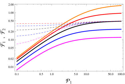
The behavior of the two independent components of the Fisher information density for the two-tracer case are plotted in Fig. 1. For small values of the effective powers ${\cal{P}}_{1}$ and ${\cal{P}}_{2}$, it is ${\cal{F}}_{1}$ which has the largest information density. However, for large values of the effective power (that is, for large enough densities of the tracers), it is ${\cal{F}}_{2}$ which carries the most information density. In the limit ${\cal{P}}_{1}\gg 1$ we see that ${\cal{F}}_{1}\rightarrow\frac{1}{2}$, while ${\cal{F}}_{2}\rightarrow\frac{1}{4}{\cal{P}}_{2}$; hence, when both ${\cal{P}}_{1}\gg 1$ and ${\cal{P}}_{2}\gg 1$, we have ${\cal{F}}_{1}\approx\frac{1}{2}$, but ${\cal{F}}_{2}\gg 1$. If ${\cal{P}}_{1}$ or ${\cal{P}}_{2}$ vanishes in some region of space, this region will not contribute with any information about their ratio (${\cal{Y}}_{2}$), although it does contribute to the usual Fisher matrix density (the one associated with ${\cal{Y}}_{1}={\cal{P}}$). When both tracers vanish in some region of space, then the whole Fisher matrix also vanishes identically.

Figure 1: Fisher matrix elements in the case of two species of tracers. The Fisher information density ${\cal{F}}_{1}$ of Eq. (16), which is associated with the total effective spectrum ${\cal{Y}}_{1}={\cal{P}}={\cal{P}}_{1}+{\cal{P}}_{2}$, is shown by the dashed lines for various values of ${\cal{P}}_{2}$ (0.5, 1, 2, 4, and 8, from the bottom up). The Fisher information density ${\cal{F}}_{2}=\frac{1}{4}{\cal{P}}_{1}{\cal{P}}_{2}/(1+{\cal{P}}_{1}+{\cal{P}}_{2})$, associated with the relative power ${\cal{Y}}_{2}={\cal{P}}_{1}/{\cal{P}}_{2}$, is shown by the solid lines.

This diagonal form of the Fisher matrix has an additional advantage: it reduces the amount of computations needed for practical applications. Instead of the $N_{t}(N_{t}-1)/2$ sums and integrations in Eq. (2.2), we only need to compute $N_{t}$ terms:

$$F_{ij}=\sum_{a=1}^{N_{t}}\int\frac{d^{3}k\,d^{3}x}{(2\pi)^{3}}\,\frac{d\log{\cal{Y}}_{a}}{d\theta^{i}}\,{\cal{F}}_{a}\,\frac{d\log{\cal{Y}}_{a}}{d\theta^{j}}\;.$$ (18)

This means if it ever becomes possible (and desirable) to divide the tracers in a survey into $100$ different types, we only need to compute the 100 terms in Eq. (18), instead of the $\sim 5.\times 10^{3}$ terms needed for the non-diagonal form of the Fisher matrix.

4 Applications to future surveys

As an application of these results, we study how the relative clusterings improve cosmological constraints for a hypothetical redshift survey that can detect three types of tracers of large-scale structure. These tracers were chosen to reproduce, as much as possible, the properties of luminous red galaxies (LRGs), emission-line galaxies (ELGs) and quasars or AGNs (QSOs). The LRG-like tracers are relatively rare, have a somewhat high bias, and are shallow ($z\lesssim 1.5$). The ELG-like tracers are more abundant, have a relatively low bias, and can be detected to higher redshifts compared to LRGs ($z\lesssim 2$). The QSO-like tracers are very rare, have a very high bias, and can be detected to very high redshifts ($z\lesssim 4$) – see, e.g., Abramo et al. (2012).

Fig. 2 shows the effective powers for each species of tracer, computed at the typical scale of $k=0.1$ $h$ Mpc^-1, for modes perpendicular to the line-of-sight ($\mu_{k}=0$). Since the effective power is a measure of shot noise (a high value of ${\cal{P}}_{\alpha}$ indicates very low shot noise), the effective powers chosen for Fig. 2 cover several different scenarios that one may encounter in real surveys.

Figure 2: Effective powers ${\cal{P}}_{R}$ (LRG-like, red in color version), ${\cal{P}}_{E}$ (ELG-like, yellow), and ${\cal{P}}_{Q}$ (QSO-like, blue), evaluated at $k=0.1\,h\,{\rm Mpc}^{-1}$, and across the line-of-sight ($\mu_{k}=0$).

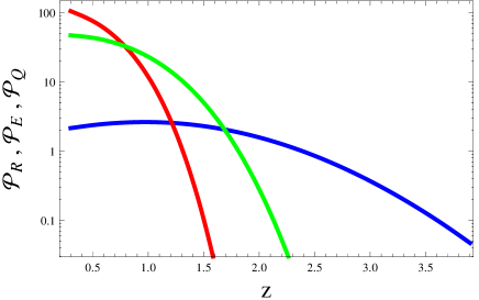
We have assumed that the survey covers $10^{4}$ deg², which, for the number densities we have considered, imply total numbers of $2\times 10^{7}$ for the LRG-like tracers, $5\times 10^{7}$ for the ELG-like tracers, and $3\times 10^{6}$ for the QSO-like tracers. We also assumed that the redshifts are accurate to $\sigma_{z}=0.001(1+z)$, and these uncertainties were factored into the Fisher matrix in the usual way, through a factor $\exp[-k^{2}\,\mu_{k}^{2}\,\sigma_{z}^{2}\,c^{2}\,H^{-2}]$ which multiplies the Fisher information density. We have also cut-off the Fourier-space integrations at $k=0.1$ $h$ Mpc^-1, in order to avoid contributions from scales where non-linear effects become essential.

We employ the same method that has been extensively used to make forecasts using the power spectrum and baryonic acoustic oscillations (BAOs) (Seo & Eisenstein, 2003; Wang, 2006). We assume that the observed power spectrum for a given tracer can be expressed in terms of a “reference” model as:

$$P_{obs}(z;k^{ref},\mu_{k}^{ref})=\left[\frac{D_{A}^{ref}(z)}{D_{A}(z)}\right]^{2}\frac{H(z)}{H^{ref}(z)}\,P_{l}(z;k^{ref},\mu_{k}^{ref})\;,$$ (19)

where:

$$P_{l}(z;k,\mu)=G^{2}(z)\left[b(z)+f(z)\,\mu^{2}_{k}\right]^{2}\,P_{l}(0;k)\;.$$ (20)

In this last equation, $P_{l}(0,k)$ denotes the linear theory, position space power spectrum at $z=0$. In Eq. (19) the wavenumbers in the fiducial model are related to those in another, arbitrary cosmology, by:

$$k^{ref}_{||}=k_{||}\frac{H^{ref}(z)}{H(z)}\quad,\quad k^{ref}_{\perp}=k_{\perp}\frac{D_{A}(z)}{D_{A}^{ref}(z)}\;.$$ (21)

Changes in the properties of $k$ and $\mu_{k}$ due to changes in the cosmological model follow from their definitions, $k=\sqrt{k_{||}^{2}+k_{\perp}^{2}}$, and $\mu^{2}_{k}=k_{||}^{2}/k^{2}$. For simplicity, we will follow Wang (2006) and absorb the normalization of the power spectrum, as well as the matter growth function, inside the prefactor of Eq. (20). This leads to the following spectrum for the species $\alpha$:

$$P_{\alpha}(z;k,\mu_{k})=\left[s_{\alpha}(z)+f_{s}(z)\,\mu^{2}_{k}\right]^{2}\,\frac{P_{l}(0;k)}{\sigma_{8}^{2}}\;,$$ (22)

where the effective bias for the tracer $\alpha$ is defined as:

$$s_{\alpha}=b_{\alpha}\times\sigma_{8}\,G(z)\;,$$ (23)

and the effective RSD parameter is given by:

$$f_{s}=f\times\sigma_{8}\,G(z)\;.$$ (24)

We will employ the subscripts $R$, $E$ and $Q$ to refer to the LRG-like tracer, the ELG-like tracer, and the QSO-like tracer respectively.

Our fiducial model is a standard, flat $\Lambda$CDM model with $\Omega_{m}=0.27$, $h=0.7$, $n_{s}=0.96$, $\Omega_{\nu}=0$ and $f_{NL}=0$. In this model, the RSD parameter is very well approximated by $f(z)=-d\log G(z)/dz\simeq\Omega_{m}^{0.55}(z)$.

Our set of parameters is the following:

$$\theta^{i}=\{\log H(z),\log D_{A}(z),s_{R}(z),s_{E}(z),s_{Q}(z),f_{s}(z),f_{NL}(z)\}\;.$$ (25)

In this paper we will discuss only the conditional errors (i.e. the reciprocals of the Fisher matrix elements), hence we have not included any global cosmological parameters such as $\Omega_{m}$, $h$, or $n_{s}$ in our analysis. It only makes sense to include global parameters, and their covariance with the parameters on each redshift slice, when we also consider priors. However, this would obfuscate the contribution that arises from the relative clusterings between the tracers, so we leave this important issue to a future paper.

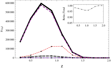
In Figs. 3 and 4 we show the Fisher information for $\log H(z)$ and $\log D_{A}(z)$ on each redshift slice. These Fisher matrix elements are related to the conditional errors by $F(\log H,\log H)=H^{2}/\sigma_{c}^{2}(H)$, and similarly for $\log D_{A}$ ($\sigma_{c}$ are the uncertainties assuming that all other parameters are kept fixed). The information in the first few redshift slices is smaller simply because the volume of the survey grows very fast with redshift.

Figure 3: Fisher matrix element $F(\log H,\log H)=H^{2}/\sigma_{c}^{2}(H)$, where $\sigma_{c}(H)$ are the conditional errors on $H$. The thick solid (black) line corresponds to the total Fisher matrix, including information from all of the tracers as well as their cross-correlations. The thin short-dashed lines correspond to the Fisher information obtained by considering only the individual tracers (in the color version, red, green and blue correspond to LRGs, ELGs and QSOs, respectively). The thick long-dashed line (gray in color version) corresponds to the Fisher information associated with the total effective volume of Eq. (16), and is subjected to the limitations imposed by cosmic variance. The long-dashed lines (dark and light purple in color version) correspond to the the contributions to the Fisher matrix which come from the relative clusterings between the different tracers, shown in Eq. (17). The inset shows the contribution of the relational information to the total information on each redshift slice.

Figure 4: Fisher matrix element $F(\log D_{A},\log D_{A})=D_{A}^{2}/\sigma_{c}^{2}(D_{A})$. The lines and the inset follow the same prescription as described in the caption for Fig. 3.

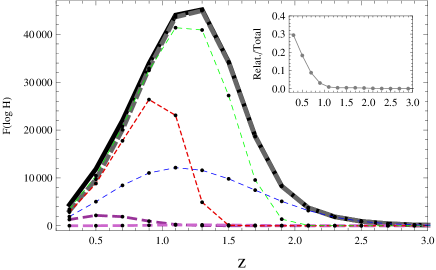
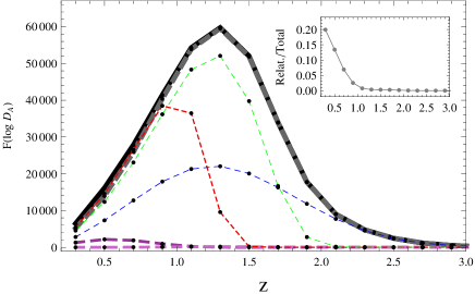
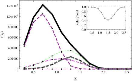
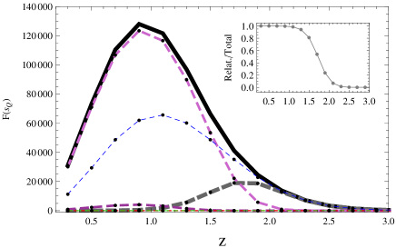
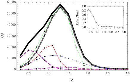
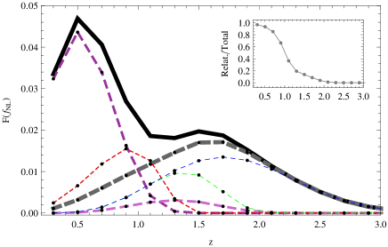
In Figs. 3-9, the thin short-dashed lines correspond to the Fisher information obtained by using only the LRG-like tracer (red in the color version), only the ELG-like tracer (green), or only the QSO-like tracer (blue). The thick solid line shows the Fisher information obtained by using all the tracers, as well as their cross-correlations; it is always above the Fisher information from the individual tracers. The thick long-dashed line (grey in color version) corresponds to the Fisher information which comes from the total effective volume of Eq. (16), and is therefore the quantity which is subject to cosmic variance. The long-dashed lines (dark and light purple in color version) correspond to the information in the relative clusterings between the three species of tracers, and are not subject to the same bounds as the effective volume – see Eq. (17). The sum of those three contributions (the thick long-dashed lines) is exactly equal to the total Fisher information (denoted by the thick solid line).

The insets (upper right corners) in Figs. 3-9 show the fraction of the Fisher information contributed by the relative clusterings between the tracers. As one can see, there is a $\sim 30\%$ enhancement in the information of $H(z)$, and a $\sim 20\%$ enhancement in the information of $D_{A}(z)$, which comes from the information in the relative amplitudes of the clusterings. These enhancementes can be understood as follows: although the prefactor of Eq. (19) contains most of the information about $H(z)$ and $D_{A}(z)$, that coefficient cancels out from the ratios between the effective powers, and therefore does not contribute anything to the Fisher information of the relative clusterings. However, the observed spectra also depend on $H(z)$ and $D_{A}(z)$ through the radial and angular components of the Fourier modes [see Eq. (21)], and that leads to some amount of information about BAOs in the relative clusterings. In fact, by increasing the redshift errors to $\sigma_{z}>0.01(1+z)$ we lose the ability to measure anisotropies in the clustering, and as a consequence the Fisher information from the relative clusterings to $H(z)$ and $D_{A}(z)$ becomes negligible.

In the case of the biases of the tracers, there is a dramatic improvement coming from the relative clusterings. In Figs. 5, 6 and 7 we show the Fisher information for the effective biases of the LRG-, ELG-, and QSO-like tracers, respectively. For the biases, the information arising from the relative clusterings is almost always dominant with respect to the information which comes from the effective volume. Moreover, including other species of tracers with different biases improves the information in the original bias by an order of magnitude, compared with the single-tracer analysis. There is a caveat, though: including other species of tracers also introduces cross-correlations between the measurements of the biases; so the conditional errors implied by the information shown in Figs. 5-7 are substantially underestimated with respect to the actual, marginalized uncertainties in those biases.

Figure 5: Fisher matrix element $F(s_{R},s_{R})=s_{R}^{2}/\sigma_{c}^{2}(s_{R})$ for the effective bias of the LRG-like tracer, $s_{R}=b_{R}\times\sigma_{8}G(z)$.

Figure 6: Fisher matrix element $F(s_{E},s_{E})=s_{E}^{2}/\sigma_{c}^{2}(s_{E})$ for the effective bias of the ELG-like tracer, $s_{E}=b_{E}\times\sigma_{8}G(z)$.

Figure 7: Fisher matrix element $F(s_{Q},s_{Q})=s_{Q}^{2}/\sigma_{c}^{2}(s_{Q})$ for the effective bias of the QSO-like tracer, $s_{Q}=b_{Q}\times\sigma_{8}G(z)$.

The most significant results are those for the effective RSD parameter, $f_{s}(z)=f(z)\,\sigma_{8}\,G(z)$, and for the local non-Gaussian parameter, $f_{NL}$. We model the non-Gaussianities in the usual way (Dalal et al., 2008), through a bias correction:

$$\Delta b_{NL}=f_{NL}(b-1)\times\frac{3\,\delta_{c}\,\Omega_{m}\,H_{0}^{2}}{c^{2}\,k^{2}\,T(k)\,G(z)}\;,$$ (26)

where $\delta_{c}=1.68$ is the critical linear density for spherical collapse, and $T(k)$ is the matter transfer function normalized to unity at large scales ($k=0$). This may not be a good approximation for quasars (Slosar et al., 2008), for which the factor $(b-1)$ in Eq. (26) should perhaps be substituted by $(b-1.6)$, but we have kept the original definition for the sake of comparison between tracers of different biases.

In Fig. 8 we show the Fisher information for $f_{s}$ on each redshift slice, and it is clear that the information from relative clusterings can enhance the information in the effective volume by up to a factor of $\sim$ 10. The largest improvement is precisely at the lowest redshift slices, which are also the ones which are most sensitive to dark energy and modified gravity models. This figure shows that, in order to measure the RSD parameter with high accuracy (both as a function and as a function of scale), we need to observe many more tracers at redshifts $z\lesssim 1$ than a simple argument based on shot noise would indicate. These results confirm and extend those of Hamaus et al. (2012).

Figure 8: Fisher matrix element for the effective redshift distortion parameter, $f_{s}(z)=f(z)\,\sigma_{8}\,G(z)$.

The Fisher information for $f_{NL}$ is shown in Fig. 9. There is a dramatic enhancement in the information at low redshifts, with respect to what we expect solely from the effective volume. In fact, the improvement is so large that it may seem at odds with the fact that non-Gaussianities are manifested through bias-dependent modifications to the transfer function on large scales. However, for the scenario that we considered in this Section, there is so much more information density in the low redshift slices (where there is a high density of tracers), which come from comparing the clusterings between the different tracers, that this more than compensates for the relatively small scales spanned by those low-$z$ slices. The bottom line is that it is possible to enhance the constraints on $f_{NL}$ by large factors. This is also consistent with the findings of Hamaus et al. (2011).

Figure 9: Fisher matrix element for local non-Gaussianity parameter $f_{NL}$.

5 Conclusions

We have shown how galaxy surveys can constrain bias-sensitive parameters to an accuracy which is not limited by cosmic variance. This emerges naturally from the multi-tracer Fisher information matrix, whose eigenvalues include both the effective volume (which is limited by cosmic variance) and the information from comparing the relative amplitudes of clustering between tracers. It is trivial to employ the methods described in this paper to forecast the power of any survey, and to any number of tracers of large-scale structure. The task of producing forecasts is further simplified due to the diagonalized form of the multi-tracer Fisher matrix.

In order to promote clarity we made several simplifying, but probably over-optimistic assumptions: e.g., we took the shot noise of auto-correlations to be Poissonian, but assumed that there is no shot noise for the cross-correlations between different tracers. We also assumed that the different tracers of large-scale structure correspond to non-overlapping halo masses, so that the biases are not correlated – and, as shown by Gil-Marín et al. (2010); Cai & Bernstein (2011a), these correlations limit the benefits of the multi-tracer approach. In the context of the formalism presented in this paper, we can go beyond these simple assumptions by considering a more realistic covariance for the counts in cells, and then computing the corresponding multi-tracer Fisher information matrix, as was carried out in Abramo (2012). A particularly useful extension would be to compute the optimal binning for the bias in terms of the distributions of halo masses, including the cross-correlations between the biases of the different tracers.

Moreover, because priors and marginalizations tend to obfuscate the different contributions that determine each constraint, we have decided to focus on the Fisher information itself, which is related to the conditional errors by $\sigma_{c}(\theta^{i})=1/\sqrt{F_{ii}}$. However, it is clear that considering several different types of tracers also brings additional covariances, so the actual constraints (after all the marginalizations and priors) will not be enhanced by the same factor. A crucial next step to our analysis would be to consider the marginalized constraints subject to some suitable sets of priors. In particular, as already shown by Cai & Bernstein (2011b), the role of lensing as a means to determine priors on the biases of different tracers of large-scale structure seems a promising way to mitigate some of the covariances inherent to multi-tracer surveys.

Our analysis shows that the parameters whose constraints have the most to gain from a multi-tracer survey are the RSD parameter, $f(z)$, and the local non-Gaussianity parameter, $f_{NL}$. For the example employed in Section 4, the Fisher information of the effective RSD parameter increases by a factor of up to $\sim 10$ when the information from relative clustering is included, which means a factor up to $\sim 3$ reduction in the conditional errors for that parameter. For $f_{NL}$, the Fisher information is boosted by an even more dramatic factor, of $\sim 20$. For the hypothetical survey and tracers that we considered, the largest gains would occur at low redshifts, because of the higher number densities of objects in the low-$z$ slices.

Our analysis also shows that it is possible to obtain enhancements in the determination of radial and angular BAOs from the relative clusterings: in the scenario we considered, these enhancements were up to $\sim 20\%$ for the Fisher information of the angular distance $D_{A}(z)$, and up to $\sim 30\%$ for the Fisher information of $H(z)$. The explanation for these enhancements comes from the fact that radial and angular BAOs are also manifested in the anisotropies of the clustering, through $\mu_{k}$ – see Eq. (21). This is in fact a multi-tracer Alcock-Paczynski test (Alcock & Paczynski, 1979), hence it depends on whether or not the redshift accuracy of the survey allows the measurement of anisotropies in the redshift-space clustering. Indeed, we have checked that for redshift errors $\sigma_{z}\gtrsim 0.01(1+z)$ there is basically no additional contribution from the relative clusterings to the Fisher informations of $D_{A}(z)$ and $H(z)$.

The key point in this paper is that whenever a redshift survey detects tracers of large-scale structure whose clustering amplitudes are different, comparisons between the clusterings tap into additional sources of information about the parameters that describe them. It may be useful to think of a “generalized bias” for each tracer, of the form $B_{\alpha}(z;k,\mu_{k})=b_{\alpha}(z;k)+f_{2}(z;k)\mu_{k}^{2}+\ldots$ , which includes as many parameters and dependencies as one may wish to consider. As long as there are sufficiently high densities of tracers with distinct (i.e., non-degenerate) biases, we can measure $B_{\alpha}(z;k,\mu_{k})$ in bins of $z$, $k$ and $\mu_{k}$ to an accuracy which is, in principle, not limited by the volume of the survey.

Acknowledgements – R.A. would like to thank FAPESP and CNPq, and K. L. would like to acknowledge the support of the Sociedade Brasileira de Física (SBF) and the American Physical Society (APS).

References

- Abbott et al. (2005) Abbott, T. et al., 2005, astro-ph/0510346
- Abell et al. (2009) Abell, P., et al., 2009, 0912.0201
- Abramo et al. (2012) Abramo, L. R., et al., 2012, MNRAS, 423, 335
- Abramo (2012) Abramo, L. R., 2012, MNRAS, 420, 3
- Adelman-McCarthy et al. (2008a) Adelman-McCarthy, J. K., et al., 2008a, VizieR Online Data Catalog, 2282, 0
- Adelman-McCarthy et al. (2008b) Adelman-McCarthy, J. K., et al., 2008b, ApJS, 175, 297
- Alcock & Paczynski (1979) Alcock, C., Paczynski, B., 1979, Nature, 281, 358
- Bardeen et al. (1986) Bardeen, J. M., Bond, J. R., Kaiser, N., Szalay, A. S., 1986, ApJ, 304, 15
- Bartolo et al. (2004) Bartolo, N., Komatsu, E., Matarrese, S., & Riotto, A., 2004, Phys. Rept., 402, 103
- Benson et al. (2000) Benson, A. J., Cole, S., Frenk, C. S, Baugh, C. M., Lacey, C. G., MNRAS, 311, 793-808
- Benítez et al. (2009) Benítez, N., et al., 2009, ApJ, 691, 241
- (12) BigBOSS: http://bigboss.lbl.gov/ .
- Blake & Glazebrook (2003) Blake, C., Glazebrook, K., 2003 ApJ, 594, 665
- Blake et al. (2011) Blake, C., et al., 2011, MNRAS, 415, 2876
- Bonoli & Pen (2008) Bonoli, S., Pen, U.-L., 2008, MNRAS, 396, 1610
- (16) BOSS: http://cosmology.lbl.gov/boss/ .
- Cai & Bernstein (2011a) Cai, Y.-C., Bernstein, G. M., MNRAS, 416, 3009
- Cai & Bernstein (2011b) Cai, Y.-C., Bernstein, G. M., MNRAS, 422, 1045
- Cai et al. (2011) Cai, Y.-C., Bernstein, G. M., Sheth, R. K., 2011, MNRAS, 412, 995
- Cole et al. (2005) Cole, S., et al., 2005, MNRAS, 362, 505
- Dalal et al. (2008) Dalal, N., Doré, O., Huterer, D., Shirokov, A., 2008, Phys. Rev., D77, 123514
- Dekel & Lahav (1999) Dekel, A., Lahav, O., 1999, ApJ, 520, 24
- Eisenstein et al. (1999) Eisenstein, D. J., Hu, W., Tegmark, M., 1999, ApJ, 518, 2
- Ellis et al. (2012) Ellis, R., Takada, M., et al., The PFS Team, 1206.0737
- Feldman et al. (1994) Feldman, H. A., Kaiser, N., Peacock, J. A., 1994, ApJ, 426, 23
- Gil-Marín et al. (2010) Gil-Marín, H., Wagner, C., Verde, L., Jimenez, R., Heavens, A., 2011, MNRAS, 407, 772
- Hamaus et al. (2011) Hamaus, N., Seljak, U., Desjacques, V., 2011, Phys. Rev., D84, 083509
- Hamaus et al. (2012) Hamaus, N., Seljak, U., Desjacques, V., 2012, Phys. Rev., D86, 103513
- Hamilton (2005a) Hamilton, A. J. S., 2005a, Lect. Notes Phys., 665, 415, astro-ph/0503603.
- Hamilton (2005b) Hamilton, A. J. S., 2005b, Lect. Notes Phys., 665, 433, astro-ph/0503604.
- Hill (2008) Hill, G. J., et al., 2008, in “Panoramic Views of the Universe”, ASP Conf. Series, 399, 115
- Linder (2005) Linder, E., 2005, Phys. Rev., D72, 043529
- McDonald & Seljak (2008) McDonald, P., Seljak, U., 2009, JCAP, 0910, 007
- (34) PAN-STARRS: http://pan-starrs.ifa.hawaii.edu/public/
- Percival et al. (2003) Percival, W. J., Verde, L., Peacock, J. A., 2004, MNRAS, 347, 645
- Raccanelli et al. (2012) Raccanelli, A., et al., 2012, 1207.0500
- Rau (2009) Rau, A., et al., 2009, Publ. Astron. Soc. Pac., 121, 1334
- Scoville et al. (2007) Scoville, N., et al., 2007, ApJS, 172, 1
- Sefusatti & Komatsu (2007) Sefusatti, E., & Komatsu, E., 2007, Phys. Rev., D76, 083004
- Seljak (2009) Seljak, U., 2009, Phys. Rev. Lett., 102, 021302
- Seljak et al. (2009) Seljak, U., Hamaus, N., Desjacques, V., 2009, Phys. Rev. Lett., 103, 091303
- Seo & Eisenstein (2003) Seo, H.-J., Eisenstein, D. J., 2003, ApJ, 598, 720
- Slosar et al. (2008) Slosar, A., Hirata, C., Seljak, U., Ho, S., Pabmanabhan, N., 2008, JCAP, 09, 31
- Slosar (2009) Slosar, A., 2009, JCAP, 03, 004
- Smith (2009) Smith, R. E., 2009, MNRAS, 400, 851
- Smith, Scoccimarro & Sheth (2009) Smith, R. E., Scoccimarro, R., Sheth, R. K., 2007, Phys. Rev., D75, 063512
- (47) SUMIRE: http://sumire.ipmu.jp/en/
- Swanson et al. (2008) Swanson, M., Tegmark, M., Blanton, M., Zehavi, I., 2008, MNRAS, 385, 1635
- Tegmark (1997) Tegmark, M., 1997, Phys. Rev. Lett., 79, 3806
- Tegmark et al. (1998) Tegmark, M., Hamilton, A. J. S., Strauss, M. A., Vogeley, M. S. , Szalay, A. S., 1998, ApJ, 499, 555
- Verde et al. (2000) Verde, L., Wang, L., Heavens, A. F., Kamionkowski, M., 2000, MNRAS, 313, 141
- Wang (2006) Wang, Y. 2006, ApJ, 647, 1
- Weinberg (2002) Berlind, A. A., Weinberg, D. H., 2002, ApJ, 575, 587
- White et al. (2008) White, M., Song, Y.-S., Percival, W. J., 2008, MNRAS, 397, 1348
- York et al. (2000) York, D. G., et al., 2000, AJ, 120, 1579