Imaginary geometry IV:\\ interior rays, whole-plane reversibility, and space-filling trees \authorJason Miller and Scott Sheffield
Abstract
We establish existence and uniqueness for Gaussian free field flow lines started at interior points of a planar domain. We interpret these as rays of a random geometry with imaginary curvature and describe the way distinct rays intersect each other and the boundary.
Previous works in this series treat rays started at boundary points and use Gaussian free field machinery to determine which chordal processes are time-reversible when . Here we extend these results to whole-plane and establish continuity and transience of these paths. In particular, we extend ordinary whole-plane SLE reversibility (established by Zhan for ) to all .
We also show that the rays of a given angle (with variable starting point) form a space-filling planar tree. Each branch is a form of for some , and the curve that traces the tree in the natural order (hitting before if the branch from is left of the branch from ) is a space-filling form of where . By varying the boundary data we obtain, for each , a family of space-filling variants of whose time reversals belong to the same family. When , ordinary belongs to this family, and our result shows that its time-reversal is .
As applications of this theory, we obtain the local finiteness of , for , and describe the laws of the boundaries of processes stopped at stopping times.
Acknowledgments. We thank Bertrand Duplantier, Oded Schramm, Wendelin Werner, David Wilson, and Dapeng Zhan for helpful discussions. We also thank several anonymous referees for many helpful comments on an earlier version of this article.
1 Introduction
1.1 Overview
This is the fourth in a series of papers that also includes [MS16d, MS16e, MS16f]. Given a real-valued function defined on a subdomain of the complex plane , constants with , and an initial point , one may construct a flow line of the complex vector field , i.e., a solution to the ODE
| (1.1) |
In [MS16d, MS16e, MS16f] (following earlier works such as [Dub09b, She, SS13, She16a]) we fixed and interpreted these flow lines as the rays of a so-called imaginary geometry, where is the starting point of the ray and is the angle. The ODE (1.1) has a unique solution when is smooth and . However [MS16d, MS16e, MS16f] deal with the case that is an instance of the Gaussian free field (GFF) on , in which case is a random generalized function (or distribution) and (1.1) cannot be solved in the usual sense. These works assume that the initial point lies on the boundary of and use tools from theory to show that, in some generality, the solutions to (1.1) can be defined in a canonical way and exist almost surely. By considering different initial points and different values for (which corresponds to the “angle” of the geodesic ray) one obtains an entire family of geodesic rays that interact with each other in interesting but comprehensible ways.
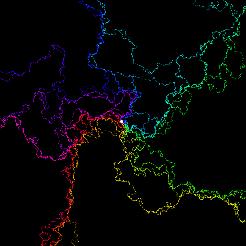
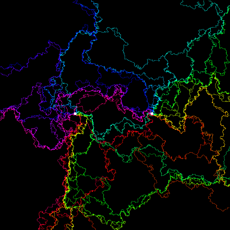
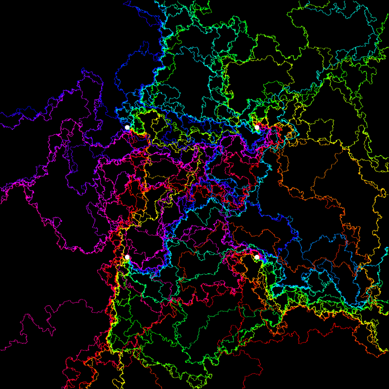
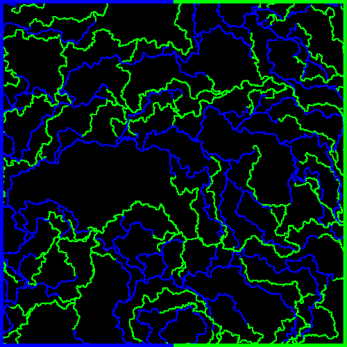
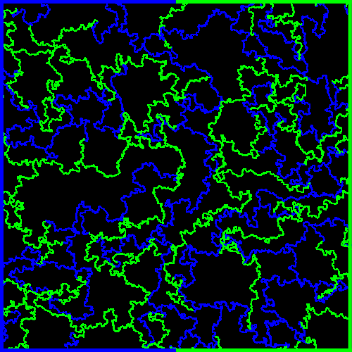
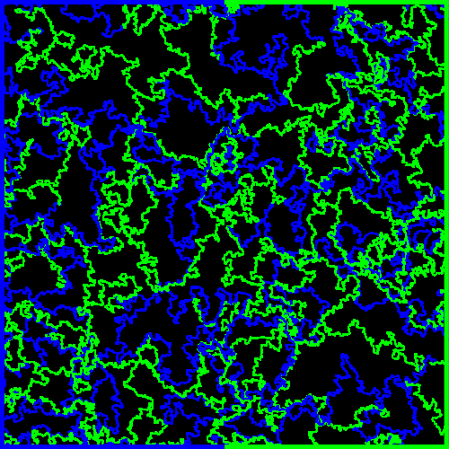
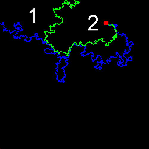
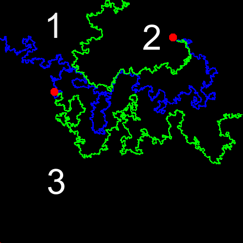
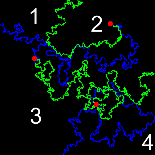
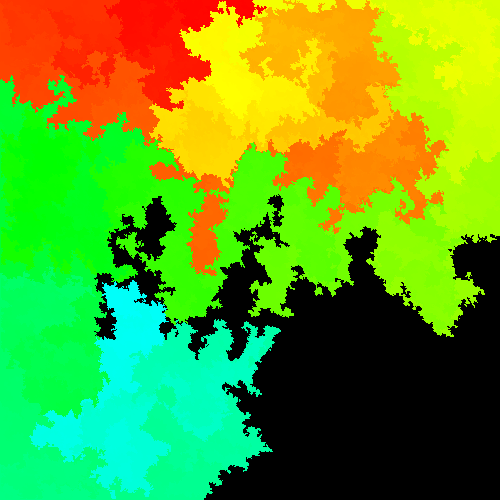
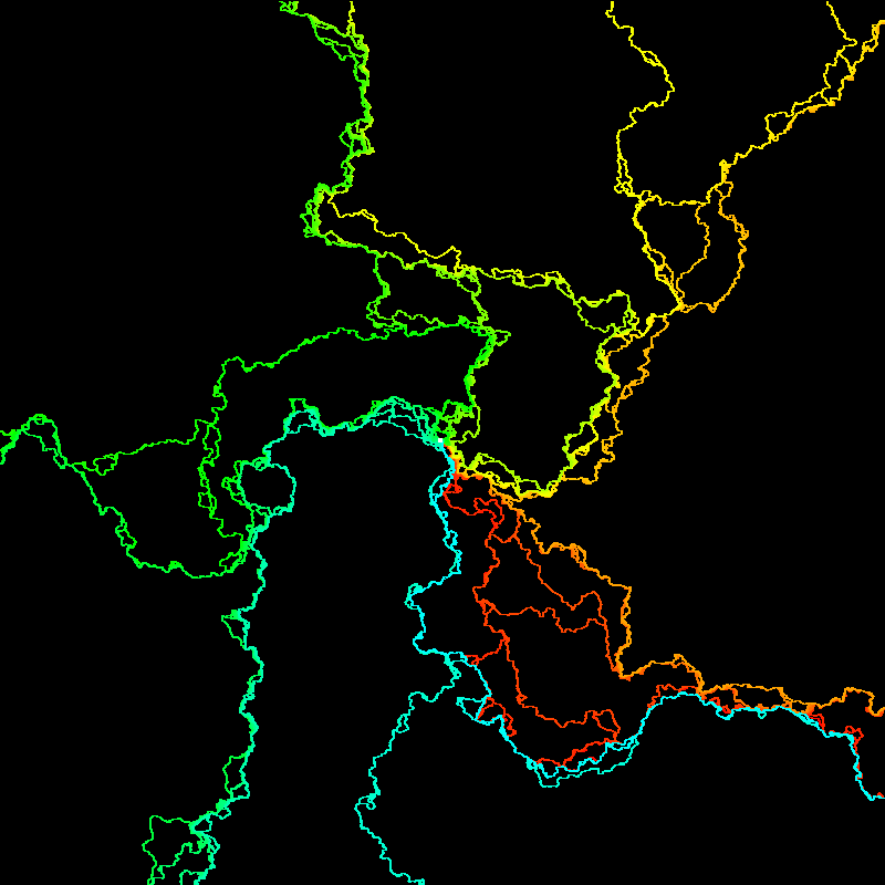
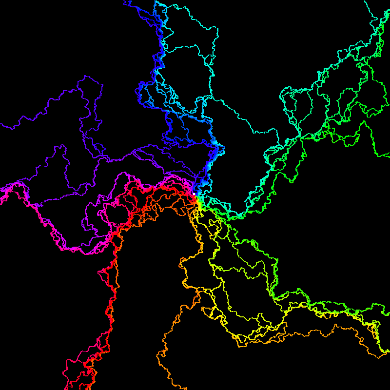
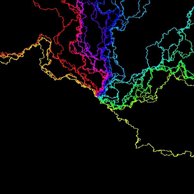
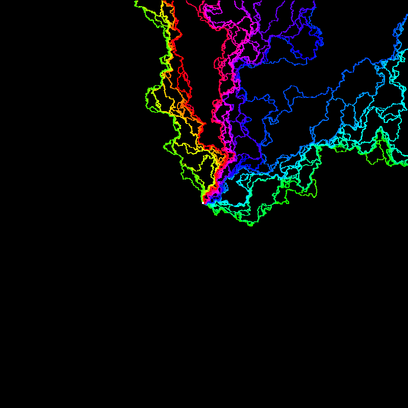
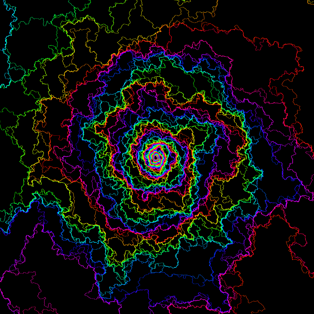
In this paper, we extend the constructions of [MS16d, MS16e, MS16f] to rays that start at points in the interior of . This provides a much more complete picture of the imaginary geometry. Figure 1.1 illustrates the rays (of different angles) that start at a single interior point when is a discrete approximation of the GFF. Figure 1.2 illustrates the rays (of different angles) that start from each of two different interior points, and Figure 1.3 illustrates the rays (of different angles) starting at each of four different interior points. We will prove several results which describe the way that rays of different angles interact with one another. We will show in a precise sense that while rays of different angles can sometimes intersect and bounce off each other at multiple points (depending on and the angle difference), they can only “cross” each other at most once before they exit the domain. (When is smooth, it is also the case that rays of different angles cross at most once; but if is smooth the rays cannot bounce off each other without crossing.) Similar results were obtained in [MS16d] for paths started at boundary points of the domain.
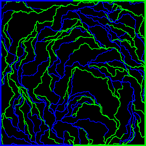
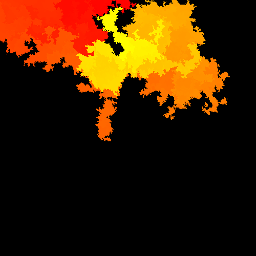
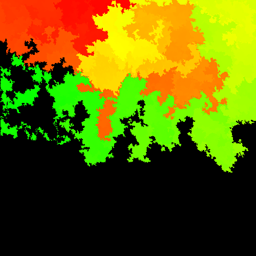
It was also shown in [MS16d] that two paths with the same angle but different initial points can “merge” with one another. Here we will describe the entire family of flow lines with a given angle (started at all points in some countable dense set). This collection of merging paths can be understood as a kind of rooted space-filling tree; each branch of the tree is a variant of , for , that starts at an interior point of the domain. These trees are illustrated for a range of values in Figure 1.4. It turns out that there is an a.s. continuous space-filling curve111We will in general write to denote an process (or variant) with and an process (or variant) with , except when making statements which apply to all values. that traces the entire tree and is a space-filling form of where (see Figure 1.5 and Figure 1.6 for an illustration of this construction for as well as Figure 1.15 and Figure 1.17 for simulations when ). In a certain sense, traces the boundary of the tree in counterclockwise order. The left boundary of is the branch of the tree started at , and the right boundary is the branch of the dual tree started at . This construction generalizes the now well-known relationship between the GFF and uniform spanning tree scaling limits (whose branches are forms of starting at interior domain points, and whose outer boundaries are forms of ) [Ken01, LSW04]. Based on this idea, we define a new family of space-filling curves called space-filling processes, defined for .
Finally, we will obtain new time-reversal symmetries, both for the new space-filling curves we introduce here and for a three-parameter family of whole-plane variants of (which are random curves in from to ) that generalizes the whole-plane processes.
In summary, this is a long paper, but it contains a number of fundamental results about and that have not appeared elsewhere. These results include the following:
-
1.
The first complete description of the collection of GFF flow lines. In particular, the first construction of the flow line rays emanating from interior points (including points with logarithmic singularities).
-
2.
The first proof that, when , the time reversal of an process is a process that belongs to the same family. It has been known for some time [RS] that itself should not have time-reversal symmetry when . However the fact that its time reversal can be described by an process was not known, or even conjectured, before the current work.
-
3.
The first proof that when the space-filling processes are well-defined, are continuous, and have time-reversal symmetry. (The reversibility of chordal was proved for in [Zha08b], for the non-boundary intersecting processes with in [Dub09a, Zha10b], for the entire class of processes in [MS16e], and for the processes with in [MS16f].)
-
4.
The first proof of the time-reversal symmetry of whole-plane processes that applies for general and . This extends the main result of [Zha15] (using very different techniques), which gives the reversibility of whole-plane for , to the entire class of whole-plane processes which have time-reversal symmetry.
- 5.
-
6.
The first proof that the conformal loop ensembles , for , are actually well-defined as random collections of loops. We also give the first proof that these random loop ensembles are locally finite and invariant under all conformal automorphisms of the domains on which they are defined. (Similar results were proved in [SW12] in the case that using Brownian loop soups.)
This paper is cited very heavily in works by the authors concerning Liouville quantum gravity, scaling limits of FK-decorated planar maps, the peanosphere, the Brownian map, and so forth. Basically, this is because there are many instances in which understanding what happens when Liouville quantum gravity surfaces are welded together turns out to be equivalent to understanding how GFF flow lines interact with each other. Moreover, the space-filling paths constructed and studied here for are the foundation of several other constructions.
To elaborate on some of these points in more detail, let us first consider the program for relating FK weighted random planar maps to -decorated Liouville quantum gravity (LQG) [DS11, She16a, She16b]. It is shown in [She16b] that it is possible to encode such a random planar map in terms of a discrete tree/dual-tree pair which are glued together along a space-filling path and that these trees converge jointly to a pair of correlated continuum random trees (CRTs) [Ald91a, Ald91b, Ald93] as the size of the map tends to . It is then shown in [DMS14] that a certain type of LQG surface decorated with a space-filling of the sort introduced in this paper (which describes the interface between a tree/dual-tree pair constructed using GFF flow lines as described above) can be interpreted as a gluing of a pair of correlated CRTs. This gives that LQG decorated with a space-filling is the scaling limit of FK weighted random planar maps where two spaces are close when the contour functions of the associated tree/dual-tree pair are close. The duality between flow line trees and space-filling curves developed here is the basis for the proofs of the main results about mating trees in [DMS14], and the results from this paper are extensively cited there. The results in this article (including results about reversibility and duality) also feature prominently in a program announced in [MS16g] and carried out in [MS15c, MS15a, MS15b, MS16b, MS16c] to construct the metric space structure of -LQG and relate it to the Brownian map.
The results here will also be an important part of the proofs of several results in joint work by the authors and with Wendelin Werner [MSW16, MS16a] about continuum analogs of FK models, conformal loop ensembles, and processes with . For example, the first proof that the processes with are continuous will be derived as a consequence of the continuity of the space-filling processes introduced here.




1.2 Statements of main results
1.2.1 Constructing rays started at interior points
A brief overview of imaginary geometry (as defined for general functions ) appears in [She16a], where the rays are interpreted as geodesics of an “imaginary” variant of the Levi-Civita connection associated with Liouville quantum gravity. One can interpret the direction as “north” and the direction as “west”, etc. Then determines a way of assigning a set of compass directions to every point in the domain, and a ray is determined by an initial point and a direction. When is constant, the rays correspond to rays in ordinary Euclidean geometry. For more general smooth functions , one can still show that when three rays form a triangle, the sum of the angles is always [She16a].

If is a smooth function, a flow line of , and a conformal transformation, then by the chain rule, is a flow line of , as in Figure 1.7. With this in mind, we define an imaginary surface222We remark that, for readers familiar with this terminology, an imaginary surface can also be understood as a simply connected domain together with a section of its orthonormal frame bundle. to be an equivalence class of pairs under the equivalence relation
| (1.2) |
We interpret as a (conformal) coordinate change of the imaginary surface. In what follows, we will generally take to be the upper half-plane, but one can map the flow lines defined there to other domains using (1.2).
Although (1.1) does not make sense as written (since is an instance of the GFF, not a function), one can construct these rays precisely by solving (1.1) in a rather indirect way: one begins by constructing explicit couplings of with variants of and showing that these couplings have certain properties. Namely, if one conditions on part of the curve, then the conditional law of is that of a GFF in the complement of the curve with certain boundary conditions. Examples of these couplings appear in [She, SS13, Dub09b, She16a] as well as variants in [MS10, HBB10, IK13]. This step is carried out in some generality in [Dub09b, She16a, MS16d]. The next step is to show that in these couplings the path is almost surely determined by the field so that we really can interpret the ray as a path-valued function of the field. This step is carried out for certain boundary conditions in [Dub09b] and in more generality in [MS16d]. Theorem 1.1 and Theorem 1.2 describe analogs of these steps that apply in the setting of this paper.
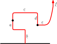
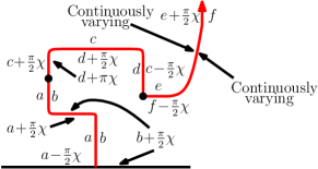
Before we state these theorems, we recall the notion of boundary data that tracks the “winding” of a curve, as illustrated in Figure 1.8. For fixed, we let
| (1.3) |
Note that for this range of values. Given a path starting in the interior of the domain, we use the term flow line boundary conditions to describe the boundary conditions that would be given by (resp. ) on the left (resp. right) side of a north-going vertical segment of the curve and then changes according to times the winding of the path, up to an additive constant in . We will indicate this using the notation of Figure 1.8. See the caption of Figure 1.9 for further explanation.
Note that if solves (1.1) when is smooth, then this will remain the case if we replace by . This will turn out to be true for the flow lines defined from the GFF as well, and this idea becomes important when we let be an instance of the whole-plane GFF on . Typically, an instance of the whole-plane GFF is defined modulo a global additive constant in , but it turns out that it is also easy and natural to define modulo a global additive multiple of (see Section 2.2 for a precise construction). When we know modulo an additive multiple of , we will be able to define its flow lines. Before we show that is a path-valued function of , we will establish a preliminary theorem that shows that there is a unique coupling between and with certain properties. Throughout, we say that a domain has harmonically non-trivial boundary if a Brownian motion started at a point in hits almost surely.
Theorem 1.1.
Fix a connected domain with harmonically non-trivial boundary and let be a GFF on with some boundary data. Fix a point . There exists a unique coupling between and a random path (defined up to monotone parameterization) started at (and stopped when it first hits ) such that the following is true. For any -stopping time , the conditional law of given is given by that of the sum of a GFF on with zero boundary conditions and a random333We recall that flow line boundary conditions are only defined up to a global additive constant in . We thus emphasize that saying that the boundary data along itself is given by flow line boundary conditions only specifies the boundary data along up to a global additive constant in . In the case that , flow line boundary conditions specify the boundary data up to a global additive constant in . In the case that has harmonically non-trivial boundary, flow line boundary conditions along specify the boundary data up to a harmonic function which is on and a multiple of on . harmonic function on whose boundary data agrees with the boundary data of on and is given by flow line boundary conditions on itself. Moreover, and are conditionally independent given . The path is simple when and is self-touching for . Similarly, if and is a whole-plane GFF (defined modulo a global additive multiple of ) there is also a unique coupling of a random path and satisfying the property described in the case above. In this case, the law of is that of a whole-plane started at . Finally, in all cases the set is local for in the sense of [SS13].
We emphasize that the harmonic function in the statement of Theorem 1.1 is not determined by in the case that and occurs before first hits . However, is determined by and the -algebra which is given by . The uniform spanning tree (UST) height function provides a discrete analogy of this statement. Namely, if one picks a lattice point and starts to explore a branch of the UST starting from back to the boundary, then the UST height function along the path is not determined by the path before the path has hit the boundary. However, if one conditions on both the path and the height function at one point along the path, then the heights are determined along the entire path even before it has hit the boundary.
In this article, we will often use the term “self-touching” to describe a curve which is both self-intersecting and non-crossing.
We will give an overview of the whole-plane and related processes in Section 2.1 and, in particular, show that these processes are almost surely generated by continuous curves. This extends the corresponding result for chordal processes established in [MS16d]. In Section 2.2, we will explain how to make sense of the GFF modulo a global additive multiple of a constant . The construction of the coupling in Theorem 1.1 is first to sample the path according to its marginal distribution and then, given , to pick as a GFF with the boundary data as described in the statement. Theorem 1.1 implies that when one integrates over the randomness of the path, the marginal law of on the whole domain is a GFF with the given boundary data. Our next result is that is in fact determined by the resulting field, which is not obvious from the construction. Similar results for “boundary emanating” GFF flow lines (i.e., flow lines started at points on the boundary of ) appear in [Dub09b, MS16d, SS13].
Theorem 1.2.
In the coupling of a GFF and a random path as in Theorem 1.1, the path is almost surely determined by viewed as a distribution modulo a global multiple of . (In particular, the path does not change if one adds a global additive multiple of to .)
Theorem 1.1 describes a coupling between a whole-plane process for and the whole-plane GFF. In our next result, we will describe a coupling between a whole-plane process for general (this is the full range of values for which ordinary makes sense) and the whole-plane GFF plus an appropriate multiple of the argument function. We motivate this construction with the following. Suppose that is a smooth function on the cone obtained by identifying the two boundary rays of the wedge . (When defining this wedge, we consider to belong to the universal cover of , on which is continuous and single-valued; thus the cone is defined even when .) Note that there is a range of angles of flow lines of in starting from and a range of angles of flow lines starting from any point . We can map to with the conformal transformation . Applying the change of variables formula (1.2), we see that is a flow line of if and only if is a flow line of . Therefore we should think of (where is a GFF) as the conformal coordinate change of a GFF with a conical singularity. The value of determines the range of angles for flow lines started at : indeed, by solving , we obtain
| (1.4) |
which exceeds zero as long as . See Figure 1.11 for numerical simulations.
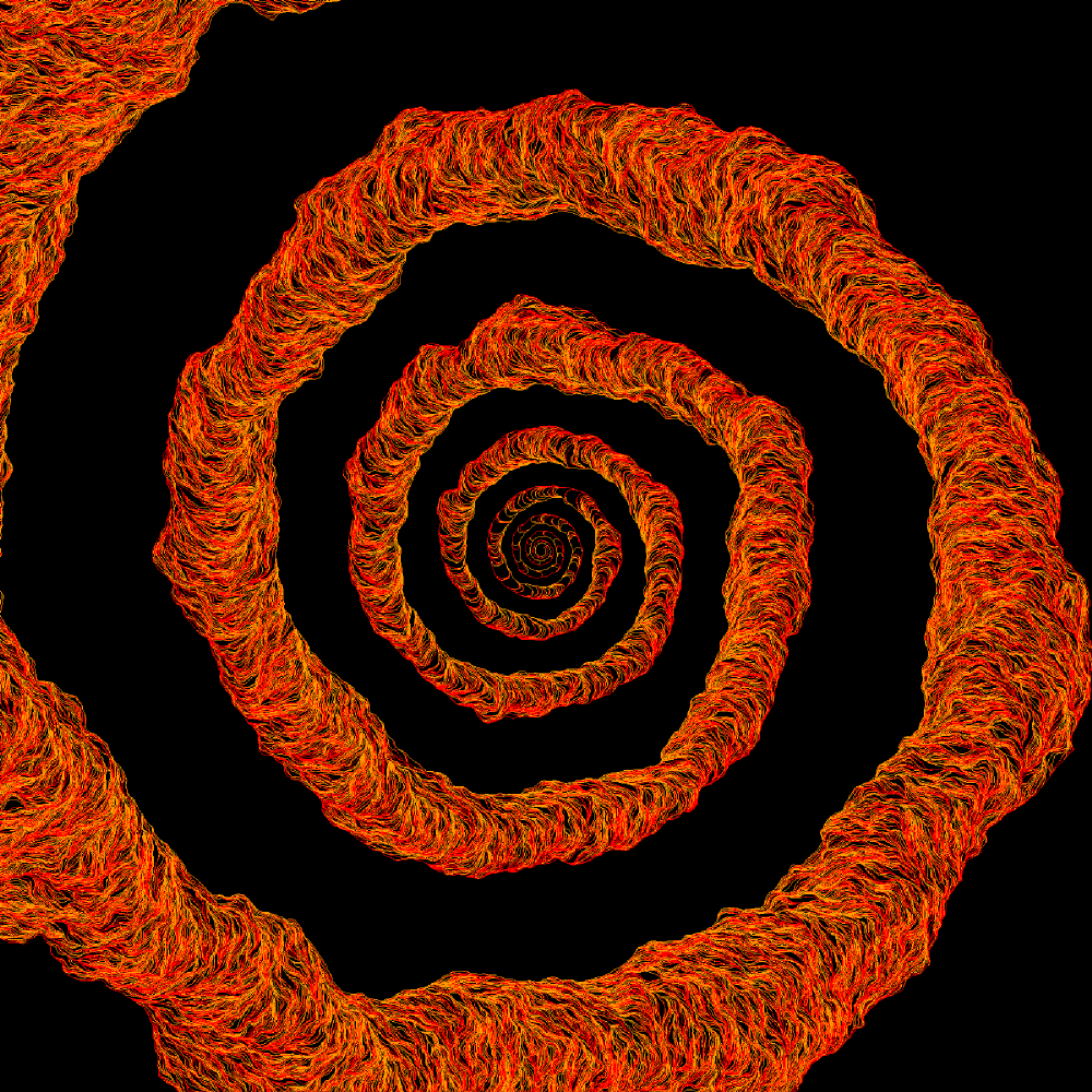
Theorem 1.4, stated just below, implies that analogs of Theorem 1.1 and Theorem 1.2 apply in the even more general setting in which we replace with , (where is as in (1.3)), , and is fixed. When and is a whole-plane GFF, the flow line of starting from is a whole-plane process where the value of depends on . Non-zero values of cause the flow lines to spiral either in the clockwise or counterclockwise () direction; see Figure 1.12. In this case, the flow line is a variant of whole-plane in which one adds a constant drift whose speed depends on . As will be shown in Section 5, the case that will arise in our proof of the reversibility of whole-plane .
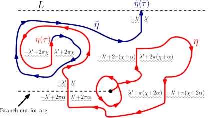
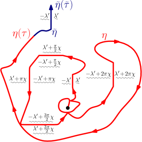
Before stating Theorem 1.4, we will first need to generalize the notion of flow line boundary conditions; see Figure 1.10. We will assume without loss of generality that the starting point for is given by for simplicity; the definition that we will give easily extends to the case . We will define a function that describes the boundary behavior of the conditional expectation of along where is a flow line and is a stopping time for . To avoid ambiguity, we will focus throughout on the branch of given by taking and we place the branch cut on . In the case that , the we defined (recall Figure 1.9) was only determined modulo a global additive multiple of since in this setting, each time the path winds around , the height of changes by . For general values of , each time the path winds around , the height of changes by , for the defined in (1.4). Therefore it is natural to describe the values of modulo global multiple of . As we will explain in more detail later, adding a global additive constant that changes the values of modulo amounts to changing the “angle” of . Since has a size “jump” along (coming from the discontinuity in ), the boundary data for will have an analogous jump.
In order to describe the boundary data for , we fix a horizontal line which lies above , we let , and be a non-self-crossing path contained in the half-space which lies below with and . We moreover assume that the final segment of is a north-going vertical line. We set the value of to be (resp. ) on the left (resp. right) side of the terminal part of and then extend to the rest of as in Figure 1.8 except with discontinuities each time the path crosses . Namely, if crosses from above (resp. below), the height increases (resp. decreases) by . Note that these discontinuities are added in such a way that the boundary data of changes continuously across the branch discontinuity. We say that a GFF on has -flow line boundary conditions (modulo ) along if the boundary data of agrees with along , up to a global additive constant in . We emphasize that this definition does not depend on the particular choice of . The reason is that although two different choices may wind around a different number of times before hitting , the difference only changes the boundary data of along by an integer multiple of .
Remark 1.3.
The boundary data for the that we have defined jumps by when passes through due to the branch cut of the argument function. If we treated and as multi-valued (generalized) functions on the universal cover of , then we could define in a continuous way on the universal cover of . However, we find that this approach causes some confusion in our later arguments (as it is easy to lose track of which branch one is working in when one considers various paths that wind around the origin in different ways). We will therefore consider to be a single-valued generalized function with a discontinuity along , and we accept that the boundary data for has discontinuities.
Theorem 1.4.
Suppose that , with as in (1.3), and . Let be a GFF on a domain . If , we assume that some fixed boundary data for on is given. If , then we let be a GFF on defined modulo a global additive multiple of . Let . Then there exists a unique coupling between and a random path starting from so that for every -stopping time the following is true. The conditional law of given is given by that of the sum of a GFF on with zero boundary conditions and a harmonic function on with -flow line boundary conditions444We recall that -flow line boundary conditions are only defined up to a global additive constant in . So, saying that the boundary data along itself is given by -flow line boundary conditions only specifies the boundary data along up to a global additive constant in . In the case that , -flow line boundary conditions specify the boundary data up to a global additive constant in . In the case that has harmonically non-trivial boundary, -flow line boundary conditions along specify the boundary data up to a harmonic function which is on and a multiple of on . along , the same boundary conditions as on , and a discontinuity along , as described in Figure 1.10. Given , and are conditionally independent. Moreover, if , , and , then the corresponding path is a whole-plane process with . Regardless of the values of and , is a.s. locally self-avoiding in the sense that its lifting to the universal cover of is self-avoiding. Finally, the random path is almost surely determined by the distribution modulo a global additive multiple of . (In particular, even when , the path does not change if one adds a global additive multiple of to .) In all cases the set is local for in the sense of [SS13].
As explained just after the statement of Theorem 1.1, the harmonic function is not determined by if occurs before has hit for the first time. However, it is determined if one conditions on both and the -algebra which is given by .
In the statement of Theorem 1.4, in the case that we interpret the statement that the conditional law of given has the same boundary conditions as on as saying that the behavior of the two fields at is the same. By this, we mean that the total variation distance of the laws of the two fields (as distributions modulo a global additive multiple of ) restricted to the complement of tends to as .
Using Theorem 1.4, for each we can generate the ray of starting from by taking to be the flow line of . The boundary data for the conditional law of given up to some stopping time is given by -flow line boundary conditions along with angle (i.e., has -flow line boundary conditions, as described in Figure 1.10). Note that we can determine the angle from these boundary conditions along since the boundary data along a north-going vertical segment of takes the form , up to an additive constant in . This is the fact that we need in order to prove that the path is determined by the field in Theorem 1.4. If we had taken the field modulo a (global) constant other than , then the boundary values along the path would not determine its angle since the path winds around its starting point an infinite number of times (see Remark 1.5 below). The range of possible angles starting from is determined by . If , then the range of angles is larger than and if , then the range of angles is less than ; see Figure 1.11. If then we can draw a ray from to instead of from to . (This follows from Theorem 1.4 itself and a coordinate change using the rule of Figure 1.7.) If then a ray started away from can wrap around and merge with itself. In this case, one can construct loops around in a natural way, but not flow lines connecting and . A non-zero value for causes the flow lines starting at to spiral in the counterclockwise (if ) or clockwise (if ) direction, as illustrated in Figure 1.12 and Figure 1.14.
Remark 1.5.
(This remark contains a technical point which should be skipped on a first reading.) In the context of Figure 1.10, Theorem 1.4 implies that it is possible to specify a particular flow line starting from (something like a “north-going flow line”) provided that the values of the field are known up to a global multiple of . What happens if we try to start a flow line from a different point ? In this case, in order to specify a “north-going” flow line starting from , we need to know the values of the field modulo a global multiple of , not modulo . If and and we know the field modulo a global multiple of , then there is no problem in defining a north-going line started at .
But what happens if and we only know the field modulo a global multiple of ? In this case, we do not have a way to single out a specific flow line started from (since changing the multiple of changes the angle of the north-going flow line started at ). On the other hand, suppose we let be a random variable (independent of ) in , chosen uniformly from the set of multiples of taken modulo (or chosen uniformly on all of if this set is dense, which happens if is irrational). Then we consider the law of a flow line, started at , of the field . The conditional law of such a flow line (given but not ) does not change when we add a multiple of to . So this random flow line from can be defined canonically even if is only known modulo an integer multiple of .
Similarly, if we only know modulo , then the collection of all possible flow lines of (where ranges over all the values in its support) starting from is a.s. well-defined.
It is also possible to extend Theorem 1.4 to the setting that .
Theorem 1.6.
Suppose that , , and . Let be a GFF on a domain and let . If , we view as a distribution defined up to a global multiple of . There exists a unique coupling between and a random path starting from so that for every -stopping time the following is true. The conditional law of given is a GFF on with -flow line boundary conditions with angle (resp. ) on the left (resp. right) side of , the same boundary conditions as on , and a discontinuity along , as described in Figure 1.10. Moreover, if , , and is a whole-plane GFF viewed as a distribution defined up to a global multiple of , then the corresponding path is a whole-plane process with . Finally, the random path is almost surely determined by provided and we know its values up to a global multiple of if .
The value is the critical threshold at or above which almost surely fills its own outer boundary. While we believe that is still almost surely determined by for , establishing this falls out of our general framework so we will not treat this case here. (See also Remark 1.21 below.) By making a coordinate change, we can grow a path from rather than from . For this to make sense, we need — this makes the coupling compatible with the setup of Theorem 1.4. In this case, is a whole-plane process from to provided . Moreover, the critical threshold at or below which the process fills its own outer boundary is . That is, the process almost surely fills its own outer boundary if and does not if .
1.2.2 Flow line interaction
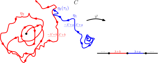
While proving Theorem 1.1, Theorem 1.2, and Theorem 1.4, we also obtain information regarding the interaction between distinct paths with each other as well as with the boundary. In [MS16d, Theorem 1.5], we described the interaction of boundary emanating flow lines in terms of their relative angle (this result is restated in Section 2.3). When flow lines start from a point in the interior of a domain, their relative angle at a point where they intersect depends on how many times the two paths have wound around their initial point before reaching the point of intersection. (This is an informal statement since paths started from interior points a.s. wind around their starting point an infinite number of times.) Thus before we state our flow line interaction result in this setting, we need to describe what it means for two paths to intersect each other at a given height or angle; this is made precise in terms of conformal mapping in Figure 1.13.
Theorem 1.7.
Assume that we have the same setup as described in the caption of Figure 1.13. On the event that hits on its right side at the stopping time for given we have that the height difference between the paths upon intersecting is a constant in . Moreover,
-
(i)
If , then crosses upon intersecting but does not subsequently cross back,
-
(ii)
If , then merges with at time and does not subsequently separate from , and
-
(iii)
If , then bounces off at time but does not cross .
The conditional law of given and is that of a GFF on with flow line boundary conditions with angle , for , on and , respectively. If, instead, hits on its left side then the same statement holds but with in place of (in particular, the range of height differences in which paths can hit is ). If the for are instead flow lines of then the same result holds except the conditional field given the paths has -flow line boundary conditions and a jump on . Finally, the same result applies if we replace with a segment of the domain boundary except that in the case that either (i) or (ii) occurs, we have that terminates upon hitting the boundary.
By dividing by , it is possible to rephrase Theorem 1.7 in terms of angle rather than height differences. The angle is called the critical angle, and the set of allowed angle gaps described in the first part Theorem 1.7 is then , with the intervals , and corresponding to flow line pairs that respectively bounce off each other, merge with each other, and cross each other at their first intersection point. We will discuss the critical angle further in Section 3.6.
We emphasize that Theorem 1.7 describes the interaction of both flow lines starting from interior points and flow lines starting from the boundary, or even one of each type. It also describes the types of boundary data that a flow line can hit. We also emphasize that it is not important in Theorem 1.7 to condition on the entire realization of before drawing . Indeed, a similar result holds if first draw an initial segment of , and then draw until it hits that segment. This also generalizes further to the setting in which we have many paths. One example of a statement of this form is the following.
Theorem 1.8.
Suppose that is a GFF on a domain , where is defined up to a global multiple of if . Fix points and angles . For each , let be the flow line of with angle starting from . Fix . For each , suppose that are non-random and that is a stopping time for the filtration
Then the conditional law of given is that of a GFF on with flow line boundary conditions with angle on each of for and the same boundary conditions as on . For each , let . On the event that is disjoint from , the continuation of stopped upon hitting is almost surely equal to the flow line of the conditional GFF given starting at with angle stopped upon hitting .
In the context of the final part of Theorem 1.8, the manner in which interacts with the other paths or domain boundary after hitting is as described in Theorem 1.7. Theorem 1.8 (combined with Theorem 1.7) says that it is possible to draw the flow lines of starting from in any order and the resulting path configuration is almost surely the same. After drawing each of the paths as described in the statement, the conditional law of the continuation of any of the paths can be computed using conformal mapping and (1.2). One version of this that will be important for us is stated as Theorem 1.11 below.
In [MS16d, Theorem 1.5], we showed that boundary emanating GFF flow lines can cross each other at most once. The following result extends this to the setting of flow lines starting from interior points. If we subtract a multiple of the argument, then depending on its value, Theorem 1.9 will imply that the GFF flow lines can cross each other and themselves more than once, but at most a finite, non-random constant number of times; the constant depends only on and . Moreover, a flow line starting from the location of the conical singularity cannot cross itself. The maximal number of crossings does not change if we subtract a multiple of the .
Theorem 1.9.
Suppose that is a domain, , and . Let be a GFF on , which is defined up to a global multiple of if . For , let be the flow line of with angle , i.e. the flow line of , starting from . Then and cross at most once (but may bounce off each other after crossing). If and , then and almost surely merge. More generally, suppose that , , is a GFF on , and , viewed as a distribution defined up to a global multiple of if , and that are flow lines of starting from with . There exists a constant such that and cross each other at most times and can cross itself at most times ( does not cross itself).
Flow lines emanating from an interior point are also able to intersect themselves even in the case that we do not subtract a multiple of the argument. In (3.17), (3.18) of Proposition 3.31 we compute the maximal number of times that such a path can hit any given point.
Theorem 1.9 implies that if we pick a countable dense subset of then the collection of flow lines starting at these points with the same angle has the property that a.s. each pair of flow lines eventually merges (if ) and no two flow lines ever cross each other. We can view this collection of flow lines as a type of planar space filling tree (if ) or a forest (if ). See Figure 1.4 for simulations which show parts of the trees associated with flow lines of angle and . By Theorem 1.2, we know that that this forest or tree is almost surely determined by the GFF. Theorem 1.10 states that the reverse is also true: the underlying GFF is a deterministic function of the realization of its flow lines started at a countable dense set. When , this can be thought of as a continuum analog of the Temperley bijection that takes spanning trees to dimer configurations which in turn come with height functions (a similar observation was made in [Dub09b]) and this construction generalizes this to other values. We note that the basic idea of using a continuum analog of Wilson’s algorithm [Wil96] to construct a planar tree of radial SLE curves (to be a scaling limit of the uniform spanning tree) appeared in Schramm’s original paper on SLE [Sch00].
Theorem 1.10.
Suppose that is a GFF on a domain , viewed as a distribution defined up to a global multiple of if . Fix . Suppose that is any countable dense set and, for each , let be the flow line of starting at with angle . If , then almost surely forms a “planar tree” in the sense that a.s. each pair of paths merges eventually, and no two paths ever cross each other. In both the case that and , the collection almost surely determines and almost surely determines .
In our next result, we give the conditional law of one flow line given another if they are started at the same point. In Section 5, we will show that this resampling property essentially characterizes the joint law of the paths (which extends a similar result for boundary emanating flow lines established in [MS16e]).
Theorem 1.11.
Suppose that is a whole-plane GFF, , , and , viewed as a distribution defined up to a global multiple of . Fix angles with and, for , let be the flow line of starting from with angle . Then the conditional law of given is that of a chordal process with
independently in each of the connected components of starting from and with force points located immediately to the left and right of the first point on the boundary of such a component visited by and targeted at last.
A similar result also holds when one considers more than two paths starting from the same point; see Proposition 3.28 as well as Figure 3.25. A version of Theorem 1.11 also holds in the case that is a GFF on a domain with harmonically non-trivial boundary. In this case, the conditional law of given is an process with the same weights independently in each of the connected components of whose boundary consists entirely of arcs of . In the connected components whose boundary consists of part of , the conditional law of is a chordal process where the weights depend on the boundary data of on (but are nevertheless straightforward to read off from the boundary data).
A whole-plane process for and is almost surely unbounded by its construction (its capacity is unbounded), however it is not immediate from the definition of that it is transient: that is, almost surely. This was first proved by Lawler for ordinary whole-plane processes, i.e. , in [Law11]. Using Theorem 1.7, we are able to extend Lawler’s result to the entire class of whole-plane processes.
Theorem 1.12.
Suppose that is a whole-plane process for and . Then almost surely. Likewise, if is a radial process for and in targeted at then, almost surely, .
1.2.3 Branching and space-filling curves
As mentioned in Section 1.1 (and illustrated in Figures 1.5, 1.6, 1.15, and 1.17) there is a natural space-filling path that traces the flow line tree in a natural order (so that a generic point is hit before a generic point when the flow line with angle from merges into the right side of the flow from with angle ). The full details of this construction (including rules for dealing with various boundary conditions, and the possibility of flow lines that merge into the boundary before hitting each other) appear in Section 4. The result is a space-filling path that traces through a “tree” of flow lines, each of which is a form of .
We will show that there is another way to construct the space-filling path and interpret it as a variant of , where . Indeed, this is true even when , in which case ordinary is not space-filling.


Before we explain this, let us recall the principle of duality (sometimes called Duplantier duality) which states that the outer boundary of an process is a certain form of . This was first proved in various forms by Zhan [Zha08a, Zha10a] and Dubédat [Dub09a]. This duality naturally arises in the context of the GFF/ coupling and is explored in [Dub09b] and [MS16d]. The simplest statement of this type is the following. Suppose that is a simply-connected domain with harmonically non-trivial boundary and fix distinct. Let be an process coupled with a GFF on as a counterflow line from to (as defined just after the statement of [MS16d, Theorem 1.1]). Then the left (resp. right) side of the outer boundary of is equal to the flow line of starting at with angle (resp. ). In the case that is boundary filling, the flow lines starting from with these angles are taken to be equal to the segments of the domain boundary which connect to in the counterclockwise and clockwise directions. More generally, the left (resp. right) side of the outer boundary of stopped upon hitting any given boundary point is equal to the flow line of starting from with angle (resp. ). In [MS16d], it is shown that it is possible to realize the entire trajectory of stopped upon hitting as the closure of the union of a countable collection of angle varying flow lines starting from whose angle is restricted to be in and is allowed to change direction a finite number of times. This path decomposition is the so-called light cone.
Our next theorem extends these results to describe the outer boundary and range of when it is targeted at a given interior point in terms of flow lines of starting from . A more explicit statement of the theorem hypotheses appears in Section 4, where the result is stated as Theorem 4.1.
Theorem 1.13.
Suppose that is a GFF on a simply-connected domain which is homeomorphic to . Assume that the boundary data is such that it is possible to draw a counterflow line from a fixed to a fixed point . (See Section 4, Theorem 4.1, for precise conditions.) If we lift to the universal cover of , then its left (resp. right) boundary is a.s. equivalent (when projected back to ) to the flow line (resp. ) of starting from with angle (resp. ). More generally, the range of stopped upon hitting is almost surely equal to the closure of the union of the countable collection of all angle varying flow lines of starting at and targeted at which change angles at most a finite number of rational times and with rational angles contained in .
As in the boundary emanating setting, we can describe the conditional law of a counterflow line given its outer boundary:
Theorem 1.14.
Suppose that we are in the setting of Theorem 1.13. If we are given and , then the conditional law of restricted to the interior connected components of that it passes through (i.e., those components whose boundaries include the right side of a directed segment, the left side of a directed segment segment, and no arc of ) is given by independent chordal processes (one process in each component, starting at the terminal point of the component’s directed and boundary segments, ending at the initial point of these directed segments).
Various statements similar to Theorem 1.13 and Theorem 1.14 hold if we start the counterflow line from an interior point as in the setting of Theorem 1.6. One statement of this form which will be important for us is the following.
Theorem 1.15.
Suppose that where , , is a whole-plane GFF, and is viewed as a distribution defined up to a global multiple of . Let be the counterflow line of starting from and targeted at . Then the left (resp. right) boundary of is given by the flow line (resp. ) starting from with angle (resp. ). The conditional law of given is independently that of a chordal process in each of the components of which are visited by . The range of is almost surely equal to the closure of the union of the set of points accessible by traveling along angle varying flow lines starting from which change direction a finite number of times and with rational angles contained in .
Recall from after the statement of Theorem 1.6 that is the critical value of at or below which fills its own outer boundary. At the critical value , the left and right boundaries of are the same.
We will now explain briefly how one constructs the so-called space-filling or processes as extensions of ordinary and processes. (A more detailed explanation appears in Section 4.) First of all, if and is such that ordinary is space-filling (i.e., ), then the space-filling is the same as ordinary . More interestingly, we will also define space-filling when and are in the range for which an ordinary path is not space-filling and the complement a.s. consists of a countable set of components , each of which is swallowed by at a finite time .
The space-filling extension of hits the points in the range of in the same order that does; however, it is “extended” by splicing into , at each time , a certain -filling loop that starts and ends at .
In other words, the difference between the ordinary and the space-filling path is that while the former “swallows” entire regions at once, the latter fills up gradually (immediately after it is swallowed) with a continuous loop, starting and ending at . We parameterize the extended path so that the time represents the area it has traversed thus far (and the path traverses a unit of area in a unit of time). Then can be obtained from the extended path by restricting the extended path to the set of times when its tip lies on the outer boundary of the region traversed thus far. In some sense, the difference between the two paths is that is parameterized by capacity viewed from the target point (which means that entire regions are absorbed in zero time and never subsequently revisited) and the space-filling extension is parameterized by area (which means that these regions are filled in gradually).
It remains to explain how the continuous -filling loops are constructed. More details about this will appear in Section 4, but we can give some explanation here. Consider a countable dense set of points in . For each we can define a counterflow line , starting at the same position as but targeted at . For , the paths and agree (up to monotone reparameterization) until the first time they separate from (i.e., the first time at which and lie in different components of the complement of the path traversed thus far). The space-filling curve will turn out to be an extension of each curve in the sense that is obtained by restricting the space-filling curve to the set of times at which the tip is harmonically exposed to .
To construct the curve, suppose that is a simply-connected domain with harmonically non-trivial boundary and fix distinct. Assume that the boundary data for a GFF on has been chosen so that its counterflow line from to is an process with ; this is the range of values in which almost surely hits both sides of . Explicitly, in the case that , , and , this corresponds to taking to be a GFF whose boundary data is given by (resp. ) on (resp. ). Suppose that is any countable, dense set of points in . For each , let (resp. ) be the flow line of starting from with angle (resp. ). As explained in Theorem 1.13, these paths can be interpreted as the left and right boundaries of . For some boundary data choices, it is possible for these paths to hit the same boundary point many times; they wind around (adding a multiple of to their heights) between subsequent hits. As explained in Section 4, we will assume that and are stopped at the first time they hit the appropriate left or right arcs of at the “correct” angles (i.e., with heights described by the multiple of that corresponds to the outer boundary of itself).
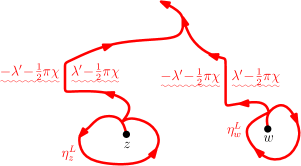
For each , divides into two parts:
-
(i)
those points in complementary components whose boundary consists of a segment of either the right side of or the left side of (and possibly also an arc of ) and
-
(ii)
those points in complementary components whose boundary consists of a segment of either the left side of or the right side of (and possibly also an arc of ).
This in turn induces a total ordering on the where we say that comes before for if is on the side described by (i). A space-filling is an almost surely non-self-crossing space-filling curve from to that visits the points according to this order and, when parameterized by conformal radius (resp. capacity), as seen from any point (resp. ) is almost surely equal to the counterflow line of starting from and targeted at .
Theorem 1.16.
Suppose that is a GFF on a Jordan domain and are distinct. Fix . If the boundary data for is as described in the preceding paragraph, then space-filling from to exists and is well-defined: its law does not depend on the choice of countable dense set . Moreover, almost surely determines the path and the path almost surely determines .
The final statement of Theorem 1.16 is really a corollary of Theorem 1.10 because determines the tree of flow lines with angle and with angle starting from the points and vice-versa. The ordering of the points in the definition of space-filling can be equivalently constructed as follows (see Figure 1.16). From points and for , we send the flow lines of with the same angle , say . If hits on its right side, then comes before and vice-versa otherwise. The ordering can similarly be constructed with the angle replaced by and the roles of left and right swapped. The time change used to get an ordinary process targeted at a given point, parameterized either by conformal radius or capacity depending on whether the target point is in the interior or boundary, from a space-filling , parameterized by area, is a monotone function which changes values at a set of times which almost surely has Lebesgue measure zero. When so that , the final statement of Theorem 1.16 can be thought of as describing the limit of the coupling of the uniform spanning tree with its corresponding Peano curve [LSW04].
The conformal loop ensembles for are the loop version of [She09, SW12]. As a consequence of Theorem 1.16, we obtain the local finiteness of the processes for . (The corresponding result for is proved in [SW12] using the relationship between s and loop-soups.)
Theorem 1.17.
Fix and let be a (bounded) Jordan domain. Let be a process in . Then is almost surely locally finite. That is, for every , the number of loops of which have diameter at least is finite almost surely.
1.2.4 Time-reversals of ordinary/space-filling
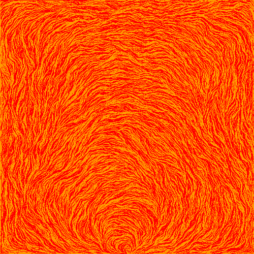
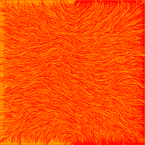
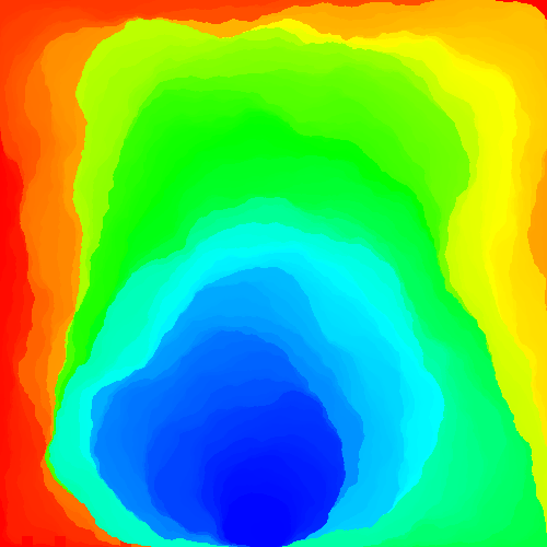

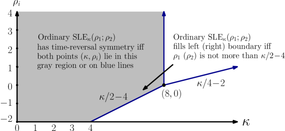
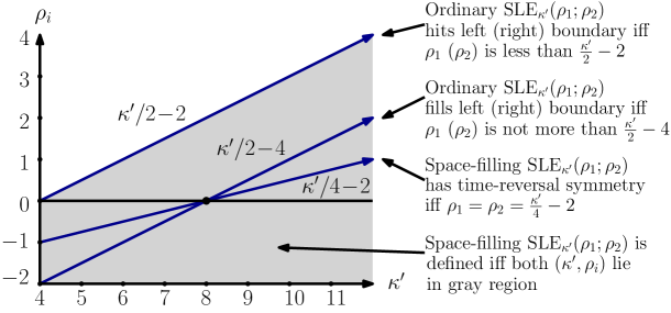
We say that a random path in a simply-connected Jordan domain from to for distinct has time-reversal symmetry if its image under any anti-conformal map which swaps and and run in the reverse direction has the same law as itself, up to reparameterization. In this article, we complete the characterization of the chordal processes that have time-reversal symmetry, as we explain in the caption of Figure 1.18. As explained earlier, throughout we generally use the symbol for values less than and for values greater than . We violate this convention in a few places (such as Figure 1.18) when we want to make a statement that applies to all . The portion of Figure 1.18 that is new to this article is the following:
Theorem 1.18.
When , ordinary has time-reversal symmetry if and only if .
The values from Theorem 1.18 are significant because for any fixed boundary point , the law of the outer boundary of an stopped upon hitting is invariant under the anti-conformal map which swaps the initial and terminal points of the path and fixes if and only if . This is a necessary condition for time-reversal symmetry and Theorem 1.18 implies that it is also sufficient. The time-reversal of an ordinary process for is not itself an process, though the time-reversal is a certain process. In particular, the result stated just below implies that it is an process. The value is significant because it is the critical threshold at or below which an process is boundary filling. It was shown in [MS16f] that if and at least one of the is strictly below , then the time-reversal of ordinary is not an process for any values of . The story is quite different if one considers space-filling , as illustrated in Figure 1.19, and formally stated as Theorem 1.19 below. (The other thresholds mentioned in the figure caption are standard Bessel process observations; see e.g. [MS16f] for more discussion.) Theorem 1.18 is a special case of Theorem 1.19.
Theorem 1.19.
The time reversal of a space-filling for is a space-filling where is the reflection of about .
1.2.5 Whole-plane time-reversal symmetry
The final result we state concerns the time-reversal symmetry of whole-plane processes for .
Theorem 1.20.
Suppose that is a whole-plane process from to for and . Then the time-reversal of is a whole-plane process from to . If is a whole-plane process for and , then the time-reversal of is a whole-plane process from to .
Our proof of Theorem 1.20 also implies the time-reversal symmetry of a flow line of as in Theorem 1.4 with for any choice of . These processes are variants of whole-plane for and in which one adds a constant drift to the driving function, which leads to spiraling, as illustrated in Figure 1.12. The proof also implies the reversibility of similar variants of whole-plane for as in Theorem 1.6 and illustrated in Figure 1.14. See Remark 5.10 in Section 5.
Remark 1.21.
When , the time-reversal of a whole-plane process for is not an process for any value of (what follows will explain why this is the case). We can nevertheless describe its time-reversal in terms of whole-plane GFF flow lines and chordal processes. Indeed, by Theorem 1.13, the left and right boundaries of are given by a pair of GFF flow lines with angles and , respectively. By Theorem 1.20, we know that has time-reversal symmetry. Moreover, by Theorem 1.11, we know that the law of given is a chordal process independently in the connected components of . Consequently, we know that the time-reversal of given the time-reversal of is independently an process in each of the connected components of by the main result of [MS16e]. Conditionally on , Theorem 1.13 gives us that the law of is that of a chordal in each of the components of part of whose boundary is traced by the right side of and the left side of . By Theorem 1.19, we thus know that the time-reversal of given the time-reversals of and is independently that of an ordinary chordal process in each of the components of ). This last statement proves our claim that the time-reversal is not a whole-plane process for any value of because the conditional law of the time-reversal of given its outer boundary is not that of an .
Remark 1.22.
We will not treat the case that is a whole-plane with and , because it does not fit into the framework of this paper as naturally. It is not hard to show that in this case the lifting of to the universal cover of has left and right boundaries that (when projected back to ) actually coincide with each other, so that . However (in contrast to the case described above) the path is not an ordinary flow line in from to . Rather, it is an angle-varying flow line, alternating between two different angles. (Using the notation of (2.4), the points on are the points hit at times when . Those hit when collides with from the right lie on flow lines of one angle. Those hit when is collides with from the left lie on flow lines of a different angle.) This angle-varying flow line is not a local set, and the conditional law of given is somewhat complicated.
2 Preliminaries
This section has three parts. First, in Section 2.1, we will give an overview of the different variants of and (chordal, radial, and whole-plane) that will be important throughout this article. We will in particular show how the continuity of whole-plane and radial processes for all and can be extracted from the results of [MS16d]. Next, in Section 2.2, we will give a brief overview of the whole-plane GFF. Finally, in Section 2.3, we will review the aspects of the theory of boundary emanating GFF flow lines developed in [MS16d] which will be relevant for this article.
2.1 processes
is a one-parameter family of conformally invariant random growth processes introduced by Oded Schramm in [Sch00] (which were proved to be generated by random curves by Rohde and Schramm in [RS05]). In this subsection, we will give a brief overview of three types of : chordal, radial, and whole-plane. More detailed introductions to can be found in many excellent surveys of the subject, e.g., [Wer04, Law05].
2.1.1 Chordal
Chordal in targeted at is the growth process associated with the random family of conformal maps obtained by solving the Loewner ODE
| (2.1) |
where is taken to be the solution to the SDE
| (2.2) |
The compact set is given by the closure of the complement of the domain of in and is the unique conformal transformation satisfying as . The points are the force points of and the are the weights. When (resp. ), is said to be a boundary (resp. interior) force point. It is often convenient to organize the into groups where the superscripts indicate whether the point is to the left or right of in or in , respectively, and we take the (resp. ) to be given in decreasing (resp. increasing) order. We also group the weights and time evolution of the force points under the Loewner flow accordingly. The existence and uniqueness of solutions to (2.2) with only boundary force points is discussed in [MS16d, Section 2]. It is shown that there is a unique solution to (2.2) until the first time that where for either or . We call this time the continuation threshold. In particular, if for all for (where we use the notation for the number of elements in the vector ), then (2.2) has a unique solution for all times . This even holds when one or both of or hold. The almost sure continuity of the trace with only boundary force points is proved in [MS16d, Theorem 1.3]. It thus follows from the Girsanov theorem [KS91] that (2.2) has a unique solution and the growth process associated with the Loewner evolution in (2.1) is almost surely generated by a continuous path, even in the presence of interior force points, up until either the continuation threshold or when an interior force point is swallowed.
2.1.2 Radial
A radial in targeted at is the random growth process in starting from a point on growing towards which is described by the random family of conformal maps which solve the radial Loewner equation:
| (2.3) |
Here, where is a standard Brownian motion; is referred to as the driving function for the radial Loewner evolution. The set is the complement of the domain of in and is the unique conformal transformation fixing with . Time is parameterized by the logarithmic conformal radius as viewed from so that for all . As in the chordal setting, radial is a generalization of radial in which one keeps track of one extra marked point. To describe it, following [SW05] we let
and
We say that a pair of processes , each of which takes values in , solves the radial equation for with a single boundary force point of weight provided that
| (2.4) |
A radial is the growth process corresponding to the solution of (2.3) when is taken to be as in (2.4). We will refer to a radial process simply a radial process. In this section, we are going to collect several facts about radial processes which will be useful for us in Section 3.1 when we prove the existence of the flow lines of the GFF emanating from an interior point.
Throughout, it will often be useful to consider the SDE
| (2.5) |
where is a standard Brownian motion. This SDE can be derived by taking a solution to (2.4) and then setting (see [She09, Equation (4.1)] for the case and ). One can easily see that (2.5) has a unique solution which takes values in if . Indeed, we first suppose that . A straightforward expansion implies that is bounded for in a neighborhood of zero (and in fact tends to zero as ). When is close to zero, this fact and the Girsanov theorem [KS91] imply that its evolution is absolutely continuous with respect to times a Bessel process of dimension and, similarly, when is close to , the evolution of is absolutely continuous with respect to times a Bessel process, also of dimension . The existence for follows by noting that, by the Girsanov theorem [KS91], its law is equal to that of with reweighted by where is the Brownian motion driving .
The existence and uniqueness of solutions to (2.4) can be derived from the existence and uniqueness of solutions to (2.5). Another approach to this for is to use [SW05, Theorem 3] to relate (2.4) to a chordal driving process with a single interior force point and then to invoke the results of [MS16d, Section 2] and the Girsanov theorem [KS91]. Pathwise uniqueness can easily be seen by considering two solutions coupled together to be driven by the same Brownian motion and then analyzing the process . In particular, if , then moves (deterministically) upwards and if then moves (deterministically) downwards. So, it must be the case that and eventually meet and do not subsequently separate. We remark that one can consider radial processes with many boundary force points as in [SW05], though we will not consider the more general case in this article. We now turn to prove the existence of a unique stationary solution to (2.4).
Proposition 2.1.
Proof.
Suppose that for are two solutions to (2.4) starting from and let . Fix . We will show that there exists and a coupling of the laws of for so that the probability that
is at most . The result will follow upon showing that this is the case. In order to prove this, it suffices to show that there is a coupling of the laws of for and so that the probability of the event that
is at most . Indeed, on the complement of this event we can couple so that for all by the uniqueness of solutions to (2.5) established just above and we have that for all .
To show that this is true, we take for to be independent and fix large. Then in each time interval of the form for there is a positive chance that stays in and stays in for the entire interval uniformly in the realization of the in the previous intervals. If is chosen sufficiently large relative to and this event occurs, then it follows from the evolution equation for that and will meet in such an interval and, at this time, and will differ by at most . Conditional on this happening, it is then a positive probability event that and will coalesce in a time which goes to zero in law as and, by this time, the distance between and will be bounded by a quantity that tends to zero in law as . It therefore follows that if is the first time that and , then decays exponentially fast in at a rate which depends only on . From this, the result follows. ∎
The following conformal Markov property is immediate from the definition of radial :
Proposition 2.2.
Suppose that is a radial process, let be the corresponding family of conformal maps, and let be the driving process. Let be any almost surely finite stopping time for . Then is a radial process whose driving function has initial condition .
We will next show that radial processes are almost surely generated by continuous curves by using [MS16d, Theorem 1.3], which gives the continuity of chordal processes.
Proposition 2.3.
Suppose that is a radial process with and . For each , we have that is almost surely generated by a continuous curve.
Proof.
It suffices to prove the result for since, as we remarked just after (2.5), the law of the process for up to any fixed and finite time is absolutely continuous with respect to the case when . Let be the driving function of a radial process with and let . We assume without loss of generality that . Let . By the conformal Markov property of radial (Proposition 2.2) and the symmetry of the setup, it suffices to prove that is generated by a continuous curve.
For each , we let . Observe from the form of (2.5) that almost surely (when , its evolution is absolutely continuous with respect to that of a positive multiple of a Bessel process of dimension larger than ). It follows from [SW05, Theorem 3] that the law of a radial process in is equal to that of a chordal process on where the weight corresponds to an interior force point located at , stopped at time . Assume that is parameterized by logarithmic conformal radius as viewed from . The Girsanov theorem implies that the law of , any fixed , is mutually absolutely continuous with respect to that of a chordal process (without an interior force point). We know from [MS16d, Theorem 1.3] that such processes are almost surely continuous, which gives us the continuity up to time . This completes the proof in the case that since does not hit at positive times because as . For the rest of the proof, we shall assume that . By sending and using that , we get the continuity up to time .
To get the continuity in the time interval , we fix and assume that is so small so the event that hits before hitting satisfies . By applying the conformal transformation , the symmetry of the setup (using that , recall (2.5)) and the argument we have described just above implies that is generated by a continuous path on . Sending implies the desired result. ∎
We will prove in Section 3.5 and Section 4 that if is a radial process with and then almost surely. This is the so-called “endpoint” continuity of radial (first established by Lawler for ordinary radial in [Law11]). We finish by recording the following fact, which follows from the discussion after (2.5).
Lemma 2.4.
Suppose that is a radial process with and . Then almost surely does not intersect and is a simple path.
Proof.
Let where is the driving pair for . By the discussion after (2.5), we know that the evolution of (resp. ) is absolutely continuous with respect to that of times a Bessel process of dimension when it is near the singularity at (resp. ). Consequently, almost surely does not hit or except possibly at time . From this, the result follows. ∎
2.1.3 Whole-plane
Whole-plane is a variant of which describes a random growth process where, for each , is compact with simply connected (viewed as a subset of the Riemann sphere). For each , we let be the unique conformal transformation with and . Then solves the whole-plane Loewner equation
| (2.6) |
Here, where is a two-sided standard Brownian motion. Equivalently, is given by the time-stationary solution to (2.4) with . Note that (2.6) is the same as (2.3). In fact, for any , the growth process for from to is a radial process in . Thus, whole-plane can be thought of as a bi-infinite time version of radial . Whole-plane is the growth process associated with (2.6) where is taken to be the time-stationary solution of (2.3) described in Proposition 2.1. As before, we will refer to a whole-plane process as simply a whole-plane process.
We are now going to prove the continuity of whole-plane processes. The idea is to deduce the result from the continuity of radial proved in Proposition 2.3 and the relationship between radial and whole-plane described just above. This gives us that for any fixed , a whole-plane restricted to is generated by the conformal image of a continuous curve. The technical issue that one has to worry about is whether pathological behavior in the way that the process gets started causes this conformal map to be discontinuous at the boundary.
Proposition 2.5.
Suppose that is a whole-plane process with and . Then is almost surely generated by a continuous curve .
Lemma 2.6.
Suppose that is a radial process with and . For each , let . Let
Then .
Proof.
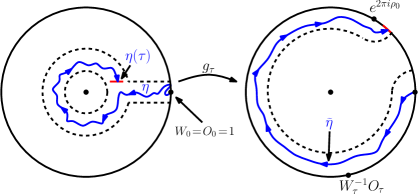
We first suppose that so that almost surely does not fill the boundary. By Proposition 2.2, the conformal Markov property for radial , it suffices to show that for each , with positive probability, the first loop that makes about does not intersect and contains . By the absolute continuity of radial and radial processes up to any fixed time , as explained in Section 2.1.2, it in turn suffices to show that this holds for ordinary radial processes. The proof of this is explained the caption of Figure 2.1. The proof for is similar. The difference is that, in this range of values, the path is almost surely boundary filling. In particular, it is not possible for the first loop that makes around the origin to be disjoint from the boundary. Nevertheless, a small modification of the argument described in Figure 2.1 implies that the inner boundary of the second loop made by around has a positive chance of being disjoint from and contain . ∎
Proof of Proposition 2.5.
We first suppose that . Fix . By the discussion in the beginning of this subsection, we know that we can express as the conformal image of a radial process. By Proposition 2.3, we know that the latter is generated by a continuous curve which, since , is almost surely non-boundary intersecting by Lemma 2.4. This implies that is generated by the conformal image of a continuous non-boundary-intersecting curve. This implies that for any , the restriction of this image to is a continuous path. The result follows since can be taken arbitrarily small.
We now suppose that and again fix . As before, we know that we can express as the image under the conformal map of a radial process . More precisely, is the complement of the unbounded connected component of . Let be the first time that . Lemma 2.6 implies that . By the almost sure continuity of the radial processes, it follows that is locally connected which implies that extends continuously to the boundary, which implies that applied to is almost surely a continuous curve. The result follows since the distribution of does not depend on since the driving function of a whole-plane process is time-stationary and we can take to be as small as we like. ∎
We finish this section by recording the following simple fact, that the trace of a whole-plane process is almost surely unbounded.
Lemma 2.7.
Suppose that is a whole-plane process with . Then almost surely.
Proof.
This follows since whole-plane is parameterized by capacity, exists for all time, and [Law05, Proposition 3.27]. ∎
2.2 Gaussian free fields
In this section, we will give an overview of the basic properties and construction of the whole-plane GFF. For a domain , we let denote the space of functions with compact support contained in . We will simply write for . We let consist of those with and write for .
Any distribution (a.k.a. generalized function) describes a linear map from to . The whole-plane GFF can be understood as a random distribution defined modulo a global additive constant in . One way to make this precise is to define an equivalence relation: two generalized functions and are equivalent modulo global additive constant if for some (i.e., for all test functions ). The whole-plane GFF modulo global additive constant is then a random equivalence class, which can be described by specifying a representative of the equivalence class. Another way to say that is defined only modulo a global additive constant is to say that the quantities are defined only for test functions . It is not hard to see that this point of view is equivalent: the restriction of the map to determines the equivalence class, and vice-versa.
If one fixes a constant , it is also possible to understand the whole-plane GFF as a random distribution defined modulo a global additive constant in . This can also be understood as a random equivalence class of distributions (with and equivalent when ). Another way to say that is defined only modulo a global additive constant in is to say that
-
1.
is well-defined for but
-
2.
for test functions , the value is defined only modulo an additive multiple of .
We can specify modulo by describing the map on and also specifying the value modulo for some fixed test function with . (A general test function is a linear combination of and an element of .)
In this subsection, we will explain how one can construct the whole-plane GFF (either modulo or modulo ) as an infinite volume limit of zero-boundary GFFs defined on an increasing sequence of bounded domains. Finally, we will review the theory of local sets in the context of the whole-plane GFF. We will assume that the reader is familiar with the ordinary GFF and the theory of local sets in this context [She07, SS13, MS16d]. Since the whole-plane theory is parallel (statements and proofs are essentially the same), our treatment will be brief.
2.2.1 Whole-plane GFF
We begin by giving the definition of the whole-plane GFF defined modulo additive constant; see also [She16a] for a similar (though somewhat more detailed) exposition. We let denote the Hilbert space closure of modulo a global additive constant in , equipped with the Dirichlet inner product
(The normalization in the definition of the Dirichlet inner product is convenient because then, for example, the dominant term in the covariance function for the GFF is given by rather than a multiple of .) Let be an orthonormal basis of and let be a sequence of i.i.d. random variables. The whole-plane GFF (modulo an additive constant in ) is an equivalence class of distributions, a representative of which is given by the series expansion
That is, for each , we can write
| (2.7) |
where is the inner product. As in the case of the GFF on a compact domain, the convergence almost surely holds for all such , and the law of turns out not to depend on the choice of [She07]. It is also possible to view as the standard Gaussian on , i.e. a collection of random variables indexed by which respect linear combinations and have covariance
Formally integrating by parts, we have that (where is, formally, the inner product of and ). Thus, for any fixed function (or generalized function) with the property that , the limit defining in (2.7) a.s. exists. (Although the limit almost surely exists for any fixed with this property, it is a.s. not the case that the limit exists for all functions with this property. However, the limit does exist a.s. for all simultaneously.) We think of as being defined only up to an additive constant in because
We can fix the additive constant, for example, by setting for some fixed with .
Suppose that are distinct with for . Then we can use either or to fix the additive constant for by setting either or . Regardless of which choice we make, as has mean zero, we have that has the Gaussian distribution with mean zero. Moreover, the variance of does not depend on the choice of for fixing the additive constant. Extending the definition of to all compactly supported test functions (not just those of mean zero) by requiring is not exactly the same as extending the definition by requiring . Each of these two extension procedures can be understood as a different mapping from a space of equivalence classes (the space of distributions modulo additive constant) to the space of distributions (where this mapping sends an equivalence class to a representative element of itself). However, note that for any fixed choice of , these two extension procedures yield distributions and that differ from one another by an additive “constant,” namely the quantity . This quantity is of course random (in the sense that it depends on ) but it is a constant in the sense that it does not depend on the spatial variable; that is, , where the quantity does not depend on .
In other words, while it is perfectly correct to say that is a random element of the space of “distributions modulo additive constant,” this does not mean that if you come up with any two different ways of fixing that additive constant (thereby producing two random distributions), the difference between the two distributions you produce will be deterministic.
Fix and with . The whole-plane GFF modulo is a random equivalence class of distributions (where two distributions are equivalent when their difference is a constant in ). An instance can be generated by
-
1.
sampling a whole-plane GFF modulo a global additive constant in , as described above, and then
-
2.
choosing independently a uniform random variable and fixing a global additive constant (modulo ) for by requiring that .
One reason that this object will be important for us is that if is a smooth function, then replacing with for does not change the north-going flow lines of the vector field . On the other hand, adding a constant in rotates all of the arrows by some non-trivial amount (so that the north-going flow lines become flow lines of angle ). Thus, while it is not possible to determine the “values” of the whole-plane GFF in an absolute sense, we can construct the whole-plane GFF modulo an additive constant in , and this is enough to determine its flow lines. These constructions will be further motivated in the next subsection in which we will show that they arise as various limits of the ordinary GFF subject to different normalizations. Before proceeding to this, we will state the analog of the Markov property for the whole-plane GFF defined either modulo an additive constant in or modulo an additive constant in .
Proposition 2.8.
Suppose that is a whole-plane GFF viewed as a distribution defined up to a global additive constant in and that is open and bounded. The conditional law of given is that of a zero-boundary GFF on plus the harmonic extension of its boundary values from to (which is only defined up to a global additive constant in ). If is defined up to a global additive constant in , then the statement holds except the harmonic function is defined modulo a global additive constant in .
We note that it is somewhat informal to refer to the “harmonic extension” of the boundary values of from to because is a distribution and not a function, so does not have “boundary values” on in a traditional sense. This “harmonic extension” is made sense of rigorously by orthogonal projection, as explained just below. The proof of Proposition 2.8 is analogous to the proof of [MS16d, Proposition 3.1], however we include it here for completeness.
Proof of Proposition 2.8.
Let be the closure of those functions in with respect to , considered modulo additive constant. Let consist of those functions in which are harmonic in (we note that whether a function is harmonic in only depends on the values of modulo a global additive constant). Then it is not difficult to see that gives an orthogonal decomposition of . Let (resp. ) be a orthonormal basis of (resp. ) and let , be i.i.d. sequences. Then we can write
The first summand has the law of a zero-boundary GFF on , modulo additive constant, and the second summand is harmonic in . We note that we can view the first summand as a zero-boundary GFF on (i.e., with the additive constant fixed) because there is a unique distribution which represents the first summand which has the property that any test function whose support is disjoint from integrates to zero against it.
The second statement in the proposition is proved similarly. ∎
The following is immediate from the definitions:
Proposition 2.9.
Suppose that is a whole-plane GFF defined up to a global additive constant in and fix . Then the laws of and are mutually absolutely continuous. The Radon-Nikodym derivative of the law of the former with respect to that of the latter is given by
| (2.8) |
where is a normalization constant. The same statement holds if is instead a whole-plane GFF defined up to a global additive constant in for . (Note: we can normalize so that for some fixed whose support is disjoint from that of .)
Proof.
Recall that if then weighting the law of by a normalizing constant times yields the law of a . We will deduce the result from this fact. We write where the are i.i.d. and is an orthonormal basis for . Fix . Then we can write . Consequently, we have that
which implies the result. ∎
2.2.2 The whole-plane GFF as a limit
We are now going to show that infinite volume limits of the ordinary GFF converge to the whole-plane GFF modulo a global additive constant either in or in for fixed, subject to appropriate normalization. Suppose that is a zero-boundary GFF on a proper domain with harmonically non-trivial boundary. Then we can consider modulo additive constant in by restricting to functions in . Fix with . We can also consider the law of modulo additive constant in for fixed by replacing with where is chosen so that .
Let (resp. ) denote the law of the whole-plane GFF modulo additive constant in (resp. for fixed; the choice of will be clear from the context).
Proposition 2.10.
Suppose that is any sequence of domains with harmonically non-trivial boundary containing such that as and, for each , let be an instance of the GFF on with boundary conditions which are uniformly bounded in . Fix . We have the following:
-
(i)
As , the laws of the distributions given by restricting the maps to (interpreted as distributions on modulo additive constant) converge in total variation to the law of the distribution (modulo additive constant) obtained by restricting the whole-plane GFF to the same set of test functions.
-
(ii)
Fix with which is constant and positive on . As , the laws of the distributions given by restricting the maps to (interpreted as distributions modulo a global additive constant in ) converge in total variation to the law of the analogous distribution (modulo ) obtained from the whole-plane GFF (as defined modulo ).
Proof.
Suppose that is a whole-plane GFF defined modulo additive constant in . By Proposition 2.8, the law of minus the harmonic extension to of its boundary values on (this difference does not depend on the arbitrary additive constant) is that of a zero-boundary GFF on .
If is large, is likely to be nearly constant on . Indeed, this can be seen as follows. Let be the density with respect to Lebesgue measure of harmonic measure in as seen from . We also let denote Lebesgue measure on . Using in the second inequality that there exists a constant such that for all and , we have that
The claim follows because it is not difficult to see that for each and there exists such that implies that for so that . We arrive at the first statement by combining this with (2.8).
Now suppose that we are in the setting of part (ii). Note that is a Gaussian random variable whose variance tends to with . Hence, modulo becomes uniform in in the limit. The second statement thus follows because, for each fixed, is independent of the family of random variables where ranges over . ∎
Proposition 2.11.
Suppose that is a domain with harmonically non-trivial boundary and is a GFF on with given boundary conditions. Fix bounded and open with . The law of considered modulo a global additive constant restricted to is mutually absolutely continuous with respect to the law of the whole-plane GFF modulo a global additive constant restricted to . Likewise, the law of considered modulo additive constant in restricted to is mutually absolutely continuous with respect to the whole-plane GFF modulo additive constant in restricted to .
Proof.
The first statement just follows from the Markov properties of the ordinary and whole-plane GFFs and the fact that adding a smooth function affects the law of the field away from the boundary in an absolutely continuous manner (Proposition 2.9). For a fixed choice of normalizing function , the laws of the whole-plane GFF modulo an additive constant in and the ordinary GFF modulo an additive constant in each integrated against are mutually absolutely continuous since the former is uniform on and the latter has the law of a Gaussian with positive variance taken modulo . The second statement thus follows from the first by taking with and which is constant and positive on and using that, with such a choice of , is independent of the family of random variables where ranges over . ∎
2.2.3 Local sets
The notion of a local set, first introduced in [SS13] for ordinary GFFs, serves to generalize the Markov property to the setting in which we condition the GFF on its values on a random (rather than deterministic) closed set. If is a planar domain and is a GFF on with some boundary conditions, then we say that a random closed set coupled with is a local set if there exists a law on pairs , where is a distribution with the property that is a.s. a harmonic function, such that a sample with the law can be produced by
-
1.
choosing the pair ,
-
2.
then sampling an instance of the zero boundary GFF on and setting .
There are several equivalent definitions of local sets given in [SS13, Lemma 3.9].
There is a completely analogous theory of local sets for the whole-plane GFF which we summarize here. Suppose that is a whole-plane GFF defined modulo a global additive constant either in or in for fixed, and suppose that is a random closed subset which is coupled with such that has harmonically non-trivial boundary. Then we say that is a local set of if there exists a law on pairs , where is a distribution with the property that is a.s. a harmonic function, such that a sample with the law can be produced by
-
1.
choosing the pair ,
-
2.
then sampling an instance of the zero boundary GFF on and setting ,
-
3.
then considering the equivalence class of distributions modulo additive constant (in or ) represented by .
The definition is equivalent if we consider as being defined only up to additive constant in or .
Using this definition, Theorem 1.1 implies that the flow line of a whole-plane GFF drawn to any positive stopping time is a local set for the field modulo . We will write for the described above (which is a harmonic function in the complement of ). In this case, the set (the flow line) a.s. has Lebesgue measure zero, so can be interpreted as a random harmonic function a.s. defined a.e. in plane (and since this is a.s. locally a function in , see the proof of [She16a, Theorem 1.1], defined modulo additive constant, writing allows us to interpret as a distribution modulo additive constant). Here we consider to be defined only up to an additive constant in (resp. ) if is a whole-plane GFF modulo additive constant in (resp. ). This function should be interpreted as the conditional mean of given and .
There is another way to think about what it means to be a local set. Given a coupling of and , we can let denote the conditional law of given . A local set determines the measurable map , which is a regular version of the conditional probability of given [SS13]. (The map is uniquely defined up to re-definition on a set of measure zero.) Let be a deterministic open subset of , and let be the measure for which . (In other words, is obtained by restricting to the event .) Using this notation, the following is a restatement of part of [SS13, Lemma 3.9]:
Proposition 2.12.
Suppose is a GFF on a domain with harmonically non-trivial boundary and is a random closed subset of coupled with . Then is local for if and only if for each open set the map is (up to a set of measure zero) a measurable function of the restriction of to .
A similar statement holds in the whole-plane setting:
Proposition 2.13.
Suppose is a whole-plane GFF defined modulo additive constant (in or ) coupled with a random closed subset of . Then is local for if and only if the map is a measurable function of the restriction of to (a function that is invariant under the addition of a global additive constant in or ).
Suppose that are local sets coupled with a GFF . Then we will write for the random, closed set which is coupled with by first sampling conditionally independently given and then taking their union. We refer to as the conditionally independent union of and . The following is a restatement of [SS13, Lemma 3.10] for the whole-plane GFF.
Proposition 2.14.
Suppose that and are local sets coupled with a whole-plane GFF , defined either modulo additive constant in or in for fixed. Then the conditionally independent union of and given is a local set for .
Proof.
In [SS13, Lemma 3.10], this statement was proved in the case that is a GFF on a domain with boundary, and the same proof works identically here. ∎
We note that in the case that and in Proposition 2.14 are -measurable, the conditionally independent union of and is almost surely equal to the usual union. By Theorem 1.2, we know that GFF flow lines are a.s. determined by the field. Therefore, we will have a posteriori that the conditionally independent union of flow lines is a.s. equal to the usual union, hence finite unions of flow lines are local. The following is a restatement of [SS13, Lemma 3.11]; see also [MS16d, Proposition 3.8].
Proposition 2.15.
Let and be connected local sets of a whole-plane GFF , defined either modulo additive constant in or in for fixed. Then is almost surely a harmonic function in that tends to zero along all sequences of points in that tend to a limit in a connected component of which consists of more than a single point. The same is also true along all sequences of points that tend to a limit in a connected component of which both consists of more than a single point and is at positive distance from either or .
Proof.
In [SS13, Lemma 3.11], this statement was proved in the case that is a GFF on a domain with boundary, and the same proof works here. ∎
We emphasize that does not depend on the additive constant and hence is defined as a function on . We will prove our results regarding the existence, uniqueness, and interaction of GFF flow lines first in the context of whole-plane GFFs since the proofs are cleaner in this setting. The following proposition provides the mechanism for converting these results into statements for the ordinary GFF.
Proposition 2.16.
Suppose that is a local set for a whole-plane GFF defined up to a global additive constant in or in for fixed. Fix open and bounded and assume that almost surely. Let be a domain in with harmonically non-trivial boundary such that with and let be a GFF on . There exists a law on random closed sets which is mutually absolutely continuous with respect to the law of such that is a local set for . Let be the function which is harmonic in which has the same boundary behavior as on . Then, moreover, the law of , up to the additive constant (taken in or in , as above), and that of are mutually absolutely continuous. Finally, if is almost surely determined by then is almost surely determined by .
Proof.
This follows from Proposition 2.11. ∎
2.3 Boundary emanating flow lines
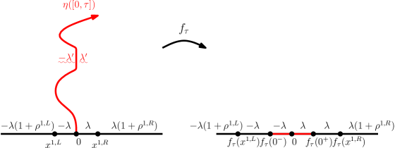
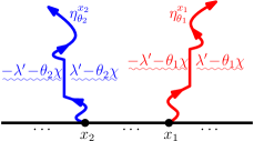
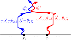
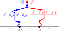
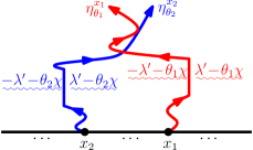
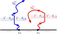
We will now give a brief overview of the theory of boundary emanating GFF flow lines developed in [MS16d]. We will explain just enough so that this article may be read and understood independently of [MS16d], though we refer the reader to [MS16d] for proofs. We assume throughout that so that . We will often make use of the following definitions and identities:
| (2.9) | ||||
| (2.10) | ||||
| (2.11) |
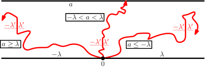
The boundary data one associates with the GFF on so that its flow line from to is an process with force points located at for and and with weights for and is
| (2.12) | ||||
| (2.13) |
This is depicted in Figure 2.2 in the special case that . For any -stopping time , the law of conditional on is a GFF in . The boundary data of the conditional field agrees with that of on . On the right side of , it is , where the terminology “winding” is explained in Figure 1.8, and to the left it is . This is also depicted in Figure 2.2.
A complete description of the manner in which GFF flow lines interact with each other is given in [MS16d, Theorem 1.5]. In particular, we suppose that is a GFF on with piecewise constant boundary data with a finite number of changes and , with . Fix angles and let be the flow line of with angle starting at , i.e. a flow line of the field , for . If , then almost surely stays to the right of . If, moreover, then almost surely does not hit and if then bounces off upon intersecting. If , then merges with upon intersecting and the flow lines never separate thereafter. If , then crosses from the right to the left of upon intersecting. After crossing, the flow lines may bounce off each other but can never cross back from the left to the right of . Finally, if , then cannot hit the right side of except in . Each of these possible behaviors is depicted in either Figure 2.3 or Figure 2.4.
It is also possible to determine which segments of the boundary that a GFF flow line can hit and this is explained in the caption of Figure 2.5. Using the transformation rule (1.2), we can extract from Figure 2.5 the values of the boundary data for the boundary segments that can hit with other orientations. We can also rephrase this in terms of the weights : a chordal process almost surely does not hit a boundary interval (resp. ) if (resp. ). See [MS16d, Lemma 5.2 and Remark 5.3]. These facts hold for all .
3 Interior flow lines
In this section, we will construct and develop the general theory of the flow lines of the GFF emanating from interior points. We begin in Section 3.1 by proving Theorem 1.1, the existence of a unique coupling between a whole-plane process for and a whole-plane GFF so that may be thought of as the flow line of starting from and then use absolute continuity to extend this result to the case that is a GFF on a proper subdomain of . Next, in Section 3.2, we will give a description of the manner in which flow lines interact with each other and the domain boundary, thus proving Theorem 1.7 and Theorem 1.9 for ordinary GFF flow lines. In Section 3.3, we will explain how the proof of Theorem 1.1 can be extended in order to establish the existence component of Theorem 1.4, i.e. the existence of flow lines for the GFF plus a multiple of one or both of and . We will also complete the proof of Theorem 1.7 and Theorem 1.9 in their full generality. Next, in Section 3.4, we will prove that the flow lines are almost surely determined by the GFF, thus proving Theorem 1.2 as well as completing the proof of Theorem 1.4. This, in turn, will allow us to establish Theorem 1.8, Theorem 1.10, and Theorem 1.11. In Section 3.5 we will use the results of Section 3.2 and Section 3.3 to prove the transience (resp. endpoint continuity) of whole-plane (resp. radial) processes for , , and . We finish in Section 3.6 with a discussion of the so-called critical angle as well as the self-intersections of GFF flow lines. Throughout, we will make frequent use of the identities (2.9)–(2.11).
3.1 Generating the coupling
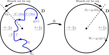
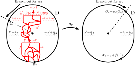
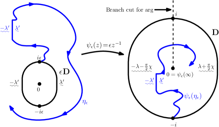
In this section, we will establish the existence of a unique coupling between a whole-plane GFF , defined modulo a global additive integer multiple of , and a whole-plane process for emanating from which satisfies a certain Markov property. Using absolute continuity (Proposition 2.16), we will then deduce Theorem 1.1. The strategy of the proof is to consider, for each , the plane minus a small disk and then take to be a GFF on with certain boundary conditions. By the theory developed in [MS16d], we know that there exists a flow line of emanating from satisfying a certain Markov property. Proposition 3.1, stated and proved just below, will allow us to identify the law of this flow line as that of a radial process. The results of Section 2.2 imply that viewed as a distribution defined up to a global multiple of converges to a whole-plane GFF defined up to a global multiple of as . To complete the proof of the existence for the whole-plane coupling, we just need to show that converges to a whole-plane process as and that the pair satisfies the desired Markov property. For proper subdomains in , the existence follows from the absolute continuity properties of the GFF (Proposition 2.16). We begin by recording the following proposition, which explains how to construct a coupling between radial with a single boundary force point with the GFF.
Proposition 3.1.
Fix and . Suppose that is a GFF on whose boundary conditions are chosen so that has the boundary data depicted in the left side of Figure 3.1 if and in the left side of Figure 3.2 if . We take the branch cut for to be on the half-infinite line from through . That is, if and (resp. ) then the boundary data for the field is equal to (resp. ) plus times the winding of on the clockwise segment of from to and (resp. ) plus times the winding of on the counterclockwise segment of from to . The boundary data is the same for other values of except it is shifted by the constant where here takes values in .
There exists a unique coupling between and a radial process in starting at , targeted at , and with a single boundary force point of weight (resp. ) if (resp. ) located at satisfying the following Markov property. For every -stopping time , the conditional law of given is that of where is a GFF on such that has the same boundary conditions as on . If , then has -flow line boundary conditions on . If , then has -flow line boundary conditions with angle (resp. ) on the left (resp. right) side of .
In this coupling, is a local set for .
In the -flow line boundary conditions in the statement of Proposition 3.1, the location of the branch cut in the argument function is the half-infinite line starting from through . This is in slight contrast to the flow line boundary conditions we introduced in Figure 1.10 in which the branch cut started from the initial point of the relevant path. The reason that we take rather than -flow line boundary conditions along the path in Proposition 3.1 in contrast to Theorem 1.4 is because in Proposition 3.1 we added to the GFF rather than subtracting it. This sign difference arises because one transforms from the whole-plane setting to the radial setting by the inversion .
As in the case of [MS16d, Theorem 1.1], we note that Proposition 3.1 can be extracted from [Dub09b]. See, in particular, [Dub09b, Theorem 5.3 and Theorem 6.4]. In order to have a proof which is independent of [Dub09b], in what follows we will indicate the modifications that need to be made to the proof of [MS16d, Theorem 1.1] in order to establish the result.
Proof of Proposition 3.1.
Following the argument of the proof of [MS16d, Theorem 1.1], in order to prove the existence of the coupling it suffices to show that the analog of [MS16d, Lemma 3.11] holds in the present setting. By [SW05, Theorem 3], it suffices to prove that the analog of [MS16d, Theorem 1.1] holds in the setting of chordal with both boundary and interior force points. Indeed, this follows because [SW05, Theorem 3] implies that a radial process has the same law as a chordal process with two force points: a boundary force point of weight with the same location as the force point of the radial process and an interior force point of weight located at the target point of the radial process. (We remark that it is possible to give a proof working purely in the radial setting, though the computations are simpler in the chordal setting with interior force points. See [MS16g, Section 5] for a proof of the so-called reverse /GFF coupling in the radial setting, which contains similar computations.)
Recall from (2.2) that the driving function for a chordal process with force points starting from with weights is given by the solution to the SDE
where is a standard Brownian motion. We let be the chordal Loewner flow driven by and let be the associated centered chordal Loewner flow. Let be the sum of the weights of the force points contained in . For each , we let
and we let
We note that if all of the are in so that all of the are in (i.e., we only have boundary force points) then and respectively agree with the corresponding definitions given in [MS16d, Equation (2.12)] and in the statement of [MS16d, Theorem 1.1].
If some of the are in , then is a multi-valued function. In order to make it single-valued (to justify our applications of Itô’s formula), we introduce branch cuts which start from each such given by a straight line to . We are now going to show that for each stopping time for which almost surely occurs before the continuation threshold is hit or one of the branch cuts is hit (in particular, before one of the interior force points is mapped to ) we have that
| (3.1) |
This is the analog of [MS16d, Theorem 1.1] in the setting of with interior force points. We will prove the result using Itô calculus.
Suppose that (so that none of the branch cuts have been hit). Applying Itô’s formula, we have that
Inserting these expressions into the explicit form of and , we thus see that
| (3.2) |
We recall that the Green’s function for on with Dirichlet boundary conditions is given by
and that gives the covariance function for the GFF on with Dirichlet boundary conditions. We let . Then an elementary calculation implies that (see, e.g., [She16a, Section 4.1])
| (3.3) |
Combining (3.2) and (3.3), we thus see that
| (3.4) |
We recall from the proof of [MS16d, Lemma 3.11] that (3.4) is the necessary equality to construct the coupling of with the GFF as its flow or counterflow line. The remainder of the existence of the coupling of with the GFF thus follows from the same argument used to prove [MS16d, Theorem 1.1].
At this point, we proved the existence of the coupling of chordal with the GFF with interior force points up until the first time that one of the branch cuts is hit or the continuation threshold is hit. We note that, given the path up to a stopping time which occurs before this happens, the boundary conditions for the conditional law of the field along the path are (resp. ) on the left (resp. right) side of the path plus times the winding. That is, they are the same as in the usual chordal coupling [MS16d, Theorem 1.1]. Note that if we move one of the branch cuts so that it passes through the path, then there will be a discontinuity in the boundary data arising because of the discontinuity of the argument function along the branch cut.
We will now explain how to extend the coupling up until the first time that one of the interior force points is separated from or the continuation threshold is hit. To this end, we let be the first time that one of the branch cuts is hit or the continuation threshold is hit. Then we know that (3.1) holds up to time .
We iterate this construction as follows. We inductively define stopping times by taking . For each , we take the branch cuts for the singularities in for to be given by vertical lines starting from each of the interior force points and through to . We then take to be the first time after that one of the branch cuts or the continuation threshold has been hit. Iteratively applying (3.1) with these new branch cuts, we thus see that (3.1) holds for . We claim that is equal to the minimum of the first time that one of the force points is cut off from (equivalently, is mapped into ) and when the continuation threshold is first hit. To see this, we suppose that is strictly less than this time. (In particular, .) It then follows that for each corresponding to an interior force point is bounded from below up to time . By the pigeon hole principle, there exists an index such that the number of times that the branch cut associated with is hit by time is infinite. Elementary considerations for conformal mapping imply that there exists such that for each such that the path hits the branch cut associated with at time . This implies that decreases to as , which is a contradiction.
We have now proved the existence of the coupling of chordal with the GFF, at least up until the first time that the process separates one of the interior force points from or the continuation threshold is hit. Note that the path may pass through the branch cuts many times before this happens. Due to the discontinuity of the argument function along each branch cut, the boundary data for the conditional law of the field given the path whenever it passes through such a branch cut jumps either up or down an amount which is equal to the corresponding jump discontinuity in the argument.
We will now explain how this implies the existence of the coupling of radial with the GFF as in the statement of the proposition, at least up until the first time that the process separates its target point from a given marked boundary point. By [SW05, Theorem 3], we know that a radial on with target point and force point located at has the same law as a chordal process with a boundary force point of weight located at and an interior force point of weight located at . Suppose that . Then by the above argument, the latter is coupled with the field given by a GFF on with boundary conditions on , on , and on ), plus the function
(Note that this function vanishes on and that and are related as in the proposition statement.) The boundary conditions are analogous in the case that . Let be the conformal map with and . Consider the field on . Note that it has boundary conditions given by plus times the winding of the boundary on , plus times the winding of the boundary on , and plus times the winding of the boundary on . More generally, if we take so that and , then the boundary data of the field is the same as in the case that except it is shifted by the constant , where here the argument takes values in . As
we find that moving the branch cut so that it passes through yields the boundary data as indicated in the statement of the proposition. (Note that the sign difference in the case that is because counterflow lines are coupled with .)
This proves the existence of the coupling of radial with the GFF as stated in the proposition, at least up until the first time that the process separates its target point from a given marked boundary point. At this time, one can then “continue” the coupling by picking a new marked boundary point inside of the complementary component containing the target point and then repeating the above with this point as the target point. Repeating this completes the proof of existence.
We now have the ingredients to complete the proof of Theorem 1.1.
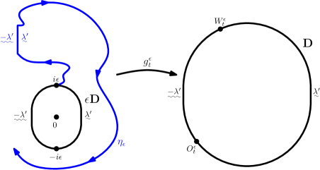
Proof of Theorem 1.1, whole-plane case.
We will first prove the existence of the coupling in the case that . For each , let be a GFF on whose boundary data is as depicted in the left side of Figure 3.3. By [MS16d, Theorem 1.1 and Proposition 3.4], it follows that we can uniquely generate the flow line of starting at . In other words, is an almost surely continuous path coupled with such that for every -stopping time , the conditional law of given is that of a GFF on whose boundary conditions agree with those of on and are given by flow line boundary conditions on . Moreover, as explained in the caption of Figure 3.3, we can read off the law of the path : it is given by that of a radial process starting at and targeted at . Let be the capacity of and assume that is defined on the time interval ; note that as . For each , we let be the unique conformal map which takes the unbounded connected component of to with and . We assume that is parameterized by capacity, i.e for every . Let be the image of the tip of in . This is the whole-plane Loewner driving function of . As explained in the caption of Figure 3.3, we know that solves the radial SDE (2.4) with ; let denote the time evolution of the corresponding force point. Proposition 2.1 states that this SDE has a unique stationary solution for and that converges weakly to as with respect to the topology of local uniform convergence. This implies that the family of conformal maps converge weakly to , the whole-plane Loewner evolution driven by , also with respect to the topology of local uniform convergence [Law05, Section 4.7]. The corresponding GFFs viewed as distributions defined up to a global multiple of converge to a whole-plane GFF which is also defined up to a global multiple of as by Proposition 2.10.
For each and each stopping time for , we can write
| (3.5) |
where is a zero boundary GFF independent of on and is the function which is harmonic on whose boundary values are on the counterclockwise segment of from to and on the clockwise segment; see Figure 3.4 for an illustration. Fix an open set and assume that is a stopping time for which almost surely occurs before the first time that hits . Then (3.5) implies that
| (3.6) |
where the right hand side is viewed as distribution on with values modulo .
The convergence of to implies that the functions converge locally uniformly to , the harmonic function on defined analogously to but with replaced by . Taking a limit as of both sides of (3.6), we see that if is any stopping time which almost surely occurs before hits then the law of
viewed as a distribution on with values modulo , is equal to that of a whole-plane GFF restricted to . The existence of the coupling then follows by applying the argument used to deduce [MS16d, Theorem 1.1] from [MS16d, Lemma 3.11].
We will now prove the uniqueness of the coupling. Suppose that is a coupling of a whole-plane GFF with values modulo and a path such that for each -stopping time we have that the conditional law of given is that of a GFF on with flow line boundary conditions on . We will prove the uniqueness by showing that necessarily has the law of a whole-plane process from to . This then determines the joint law of the pair because the Markov property determines the conditional law of given . Fix and let be the unique conformal map which takes the unbounded component of to with sent to and with positive derivative at . Then we know that can be written as the sum of a GFF on minus with boundary conditions on as in the statement of Proposition 3.1. Moreover, with , the Markov property for the pair implies that the pair satisfies the analogous Markov property (i.e., as described in the statement of Proposition 3.1). The uniqueness component of Proposition 3.1 then implies that has the law of a radial process in hence has the law of a radial process in the unbounded component of . Sending implies that has the law of a whole-plane process from to . ∎
Proof of Theorem 1.1, existence for general domains.
We will now extend the existence of the coupling to general domains ; we will defer the proof of uniqueness of the coupling until we prove Theorem 1.2 later on. The key observation is that the law of (modulo a global multiple of ) in a small neighborhood of zero changes in an absolutely continuous way when we replace with . Hence, we can couple the path with the field as if the domain were , at least up until the first time the path exits this small neighborhood (see also the discussion just after [MS16d, Lemma 3.6] regarding the Markov property for GFF flow lines when performing this type of change of measure in the context of boundary emanating flow lines). The actual value of the field on the boundary of (as opposed to just the value modulo a global multiple of ) is then a Gaussian random variable restricted to a discrete set of possible values. See Proposition 2.16. Once the path has been drawn to a stopping time (where the path is parameterized by capacity), the usual coupling rules [MS16d, Theorem 1.1 and Theorem 1.2] allow us to extend it uniquely. ∎
So far we have shown that there is a unique coupling between a path and a whole-plane GFF with values modulo such that the conditional law of given up to any -stopping time is that of GFF in with flow line boundary conditions on and is local for . We proved the existence of the coupling in the case of general domains by starting with the construction in the whole-plane case and then using absolute continuity. One could worry that there are other possible laws. This will be ruled out as a byproduct of our proof of Theorem 1.2 below. Unless explicitly stated otherwise, we shall assume throughout in what follows that a flow line on a bounded domain has the law as constructed just above (i.e., induced from the whole-plane coupling).
Suppose that is a GFF on with values modulo , are distinct, and that are flow lines of starting from , respectively, taken to be conditionally independent given . Suppose that is a stopping time for . Then we know that is a flow line for the GFF on given by given . Indeed, this follows because we know that for each -stopping that the conditional law of given both and is that of a GFF on with flow line boundary conditions on and . We claim that the coupling of with the GFF on given is the same as the one constructed in the proof of the existence component of Theorem 1.1 given just above. (This will be important in some of our conditioning arguments in the proof of Theorem 1.7, before we complete the proof of the uniqueness component of Theorem 1.1 for bounded domains given below.) Suppose that is an open set which contains but not . The locality of implies that the conditional law of up until exiting given is a function of the restriction of to . Moreover, our construction in the proof of the existence component of Theorem 1.1 given just above yields that the conditional law of the flow line given up until exiting a subdomain with boundary disjoint from is given by the same function of the values of the restriction of to . This, in turn, implies the claim.
Remark 3.2.
The proof of Theorem 1.1 implies that in the special case that is a proper domain in with harmonically non-trivial boundary, the law of stopped before hitting is absolutely continuous with respect to that of a whole-plane process. If , then is in fact a whole-plane . In particular, intersects itself if and only if by Lemma 2.4.
Remark 3.3.
In the case that , if we replace the whole-plane GFF in the proof of Theorem 1.1 given just above with , viewed as a distribution defined modulo a global multiple of , the same argument yields the existence of a coupling where is a whole-plane for starting from with
satisfying the analogous Markov property (the conditional law of the field given a segment of the path is a GFF off the path with -flow line boundary conditions; recall Figure 1.10). In order for this to make sense, we need to assume that so that . The same proof also yields the existence of a coupling where is a whole-plane for starting from with
satisfying the analogous Markov property provided .
3.2 Interaction
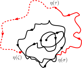
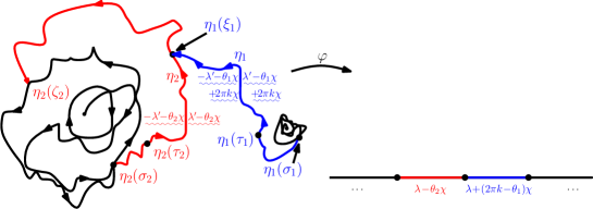
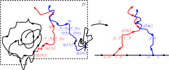
In this subsection, we will study the manner in which flow lines interact with each other and the domain boundary in order to prove Theorem 1.7 and Theorem 1.9 for ordinary GFF flow lines. The strategy to establish the first result is to reduce it to the setting of boundary emanating flow lines, as described in Section 2.3 (see Figure 2.3 and Figure 2.4 as well as [MS16d, Theorem 1.5]). This will require three steps.
-
1.
In Section 3.2.1, we will show that the so-called tails of flow lines — path segments in between self-intersection times — behave in the same manner as in the boundary emanating regime. This is made precise in Proposition 3.5; see Figure 3.6 and Figure 3.7 for an illustration of the setup and proof of this result.
- 2.
-
3.
In Section 3.2.3, we will explain how this completes the proof of our description of the manner in which flow lines interact. At a high level, the result follows in the case of flow lines starting from interior points because in this case the interaction of any two flow lines reduces to the interaction of flow line tails. The proof for the case in which a flow line starting from an interior point interacts with a flow line starting from the boundary follows from the same argument because, as it will not be hard to see from what follows, it is also possible to decompose a flow line starting from the boundary into a union of overlapping tails of flow lines starting from interior points. This result is stated precisely as Proposition 3.7.
Remark 3.4.
At this point in the article we have not proved Theorem 1.2, that flow lines of the GFF emanating from interior points are almost surely determined by the field, yet throughout this section we will work with more than one path coupled with the GFF. We shall tacitly assume that the paths are conditionally independent given the field. That is, when we refer to the flow line of a given angle and starting point, and the flow line of another angle and starting point, we at this point assume only that the laws of these paths are conditionally independent given the field (since we have not yet shown that the flow line is a deterministic function of the field). We also emphasize that, by the uniqueness theory for boundary emanating flow lines [MS16d, Theorem 1.2] and absolute continuity [MS16d, Proposition 3.4], once we have drawn an infinitesimal segment of each path, the remainder of each of the paths is almost surely determined by the field. The only possible source of randomness is in how the path gets started.
3.2.1 Tail interaction
Suppose that is a domain and let be a GFF on with given boundary conditions; if then we take to be a whole-plane GFF defined up to a global multiple of . Fix , , and let be the flow line of starting at with angle . This means that is the flow line of starting at . Let be a stopping time for at which almost surely does not intersect its past, i.e. is not contained in . We let be the largest time before at which intersects its past and . By Proposition 2.5, we know that is almost surely continuous, hence . We call the path segment the tail of associated with the stopping time and will denote it by (see Figure 3.5). The next proposition, which is illustrated in Figure 3.6, describes the manner in which the tails of flow lines interact with each other up until is disconnected from the initial point of one of the tails.
Proposition 3.5.
Let be a GFF on defined up to a global multiple of . Suppose that and . For , we let be the flow line of starting at with angle and let be a stopping time for such that almost surely. Let be the starting and ending times for the tail for as described above. Let and let be the event that , , and that hits on its right side at time . Let be the height difference of the tails upon intersecting, as defined in Figure 1.13. Then .
Let be a stopping time for for and let be the event that for is not disconnected from by . Let for . On , we have that:
-
(i)
If , then crosses upon intersecting and does not subsequently cross back,
-
(ii)
If , then merges with and does not subsequently separate from upon intersecting, and
-
(iii)
If , then bounces off but does not cross .
Finally, the conditional law of given for on is that of a GFF on whose boundary data on for is given by flow line boundary conditions with angle . If hits on its left rather than right side, the same result holds but with in place of (so the range of values for where can hit is ).
Proof.
The proof is contained in the captions of Figure 3.6 and Figure 3.7, except for the following two points. First, the reason that we know that is a local set for is that, if we draw each of the paths up until any fixed stopping time, then their union is local by Proposition 2.14 (recall that we took the paths to be conditionally independent given ). Their continuations are local for and, moreover, almost surely determined by the conditional field given these initial segments (recall Remark 3.4). Hence the claim follows from [MS16d, Lemma 6.2]. Second, the reason that the boundary data for given and is given by flow line boundary conditions is that we were working on the event that . Consequently, we can get the boundary data for given and by using Proposition 2.15 to compare to the conditional law of given and given separately. The reason that the boundary data for the conditional law of given and has flow line boundary conditions (without singularities at intersection points) is that we can apply the boundary emanating theory from [MS16d]. ∎
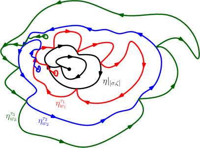
The reason that the statement of Proposition 3.5 is more complicated than the statement which describes the interaction of boundary emanating flow lines [MS16d, Theorem 1.5] is that we needed a way to encode the height difference between and upon intersecting since the paths have the possibility of winding around their initial points many times after the stopping times and .
3.2.2 Decomposing flow lines into tails
Now that we have described the interaction of tails of flow lines, we turn to show that it is possible to decompose a flow line into a union of overlapping tails. This combined with Proposition 3.5 will lead to the proof of Theorem 1.7. Suppose that is a non-crossing path starting at . Then we say that has made a clean loop at time around if the following is true. With , we have that is a simple loop which surrounds and does not intersect . Note that Lemma 2.6 implies that GFF flow lines for , which we recall are given by whole-plane processes for for (and if , their law is absolutely continuous with respect to that of whole-plane up until hitting ), almost surely contain arbitrarily small clean loops.
Proposition 3.6 (Tail Decomposition: Interior Regime).
Assume that . Suppose that is a whole-plane GFF defined up to a global multiple of . Fix , , and let be the flow line of starting from with angle . Let be any stopping time for such that has made a clean loop around at time , as described just above. Then we can decompose into a union of overlapping tails of flow lines where starts from and has angle with the following properties:
-
(i)
For every , the starting point of the flow line of with angle has rational coordinates and is contained in a bounded complementary component of (we take ),
-
(ii)
There exists stopping times for such that, for each , the outer boundary of is almost surely equal to the outer boundary of , and
-
(iii)
For each , conditional on , is independent of restricted to the unbounded complementary connected component of .
We emphasize that in the statement of Proposition 3.6, the flow lines are taken to be conditionally independent of given . The starting points of the flow lines are rational, as stated in the proposition statement, but are random and depend on , , and the collection of flow lines starting at with rational coordinates (as in the statement, all flow lines are taken to be conditionally independent given ). We note that the tail of a flow line can either be a simple curve or a simple loop (i.e., homeomorphic to ) depending on when the first intersection time of the path with itself occurs. It is implicit in the second condition of Proposition 3.6 that the tails are of the latter type.
The reason that we assume in the statement of Proposition 3.6 is that if then is non-self-intersecting hence its entire trace is itself a tail. Fix and let be the first time after that makes a clean loop around . It is a consequence of Lemma 2.6 that almost surely and it follows from Proposition 2.1, which gives the stationarity of the driving function of , that the distribution of does not depend on . Consequently, for every and we can choose our stopping time in Proposition 3.6 such that . The techniques we use to prove Proposition 3.6 will also allow us to show that boundary emanating flow lines similarly admit a decomposition into a union of overlapping tails. This will also us to describe the manner in which boundary emanating flow lines interact with flow lines starting from interior points using Proposition 3.5.
Proposition 3.7 (Tail Decomposition: Boundary Regime).
Suppose that is a GFF on a domain with harmonically non-trivial boundary and let be a flow line of starting from with angle . Then we can decompose into a union of overlapping tails with the following properties:
-
(i)
For every , the starting point of has rational coordinates and
-
(ii)
The range of is contained in almost surely.
If, in addition, is self-intersecting then properties (ii) and (iii) as described in Proposition 3.6 hold with .
In order to establish Proposition 3.6 and Proposition 3.7, we need to collect first the following three lemmas. The third, illustrated in Figure 3.10, implies that if we start a flow line close to the tail of another flow line with the same angle, then with positive probability the former merges into the latter at their first intersection time and, moreover, this occurs without the path leaving a ball of fixed radius.
Lemma 3.8.
Suppose that is a whole-plane GFF defined up to a global multiple of . Let be the flow line of starting from and any almost surely finite stopping time for such that almost surely. Given , let be any simple path starting from such that is contained in the unbounded connected component of . Fix and let be the -neighborhood of . Finally, let
Then .
Proof.
Given , we let be a simply connected domain which contains , is contained in , and such that there exists with and .
We can construct explicitly as follows. Let be the unique conformal map from the unbounded component of to with as . As is almost surely continuous, it follows that extends to be a homeomorphism from the boundary of its domain (viewed as prime ends) to . Therefore is a continuous path in and is a relatively open neighborhood of . Moreover, as is almost surely a non-intersection time for , we have that has positive distance from the image under of an intersection point of . Therefore we can find which is relatively open which is contained in , contains , and which contains a neighborhood in of which is disjoint from images of self-intersection points of . By choosing appropriately, we may further assume that for some small. We can also take to be the intersection with of a domain with polygonal boundary with vertices with rational coordinates. We then take and note that satisfies the desired properties.
Fix with . Let be a GFF on whose boundary data along agrees with that of (up to an additive constant in ) and whose boundary data on is such that the flow line of starting from is an ordinary chordal process in targeted at . Let and note that almost surely since terminates at . Since almost surely, it follows that we can pick sufficiently small so that . The result follows since by [MS16d, Proposition 3.4] the law of restricted to is absolutely continuous with respect to the law of given restricted to the same set, up to an additive constant in , and that almost surely. ∎
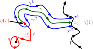
Lemma 3.9.
Suppose that is a GFF on a proper subdomain whose boundary consists of a finite, disjoint union of continuous paths, each with flow line boundary conditions of a given angle (which can change from path to path), , and is the flow line of starting from . Fix any almost surely positive and finite stopping time for such that and almost surely. Given , let be any simple path in starting from such that is contained in the unbounded connected component of , , and . Moreover, assume that if we extended the boundary data of the conditional law of given along as if it were a flow line then the height difference of and upon intersecting at time is in the admissible range for hitting. Fix , let be the -neighborhood of in , and let
Then .
We recall that the admissible range of height differences for hitting is if is hitting on the right side and is on the left side. See Figure 3.9 for an illustration of the proof.
Proof of Lemma 3.9.
Let be the connected component of which contains . Let (resp. ) be a simple path in which connects a point on the left (resp. right) side of to a point on the same side of hit by at time , say (resp. ), and does not intersect . Assume that . Let be the region of which is surrounded by and . Let be a GFF on whose boundary data agrees with that of on and on and is otherwise given by flow line boundary conditions. We choose the angles of the boundary data on so that the flow line of starting from is an process targeted at and the force points are located at and . Moreover, since we assumed that if we continued the boundary data for given along as if it were a flow line then it is in the admissible range for hitting (and by our construction, the same is true for both and ). Let . Since almost surely, it follows that we can pick sufficiently small so that . The result follows since the law of restricted to is absolutely continuous with respect to the law of given restricted to the same set and almost surely. ∎
Our first application of Lemma 3.9 is the following, which is an important ingredient in the proof of Proposition 3.6.
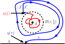
Lemma 3.10.
Suppose that is a GFF on with constant boundary data as depicted in Figure 3.10. Let be the flow line of starting at and let . Let be the event that hits with a height difference of and let . There exists such that
| (3.7) |
The same likewise holds when is replaced with .
Proof.
See Figure 3.10 for an illustration of the setup. We let be the first time that hits . We let be a simple path in starting from which winds around precisely times until hitting . We choose so that if we continued the boundary data of along , the height difference of upon intersecting is zero. The lemma then follows from Lemma 3.9. ∎
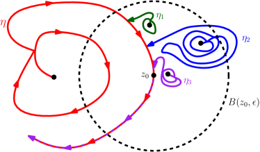
By repeated applications of Lemma 3.10, we are now going to prove that the restriction of the tail of a flow line associated with the stopping time and ending at to the time interval almost surely is represented as the tail of a flow line whose initial point is close to and which merges into without leaving a small ball centered at . See Figure 3.11 for an illustration of the setup of this result.
Lemma 3.11.
Suppose that is a GFF on defined up to a global multiple of , let be the flow line of starting from , and let be a stopping time for such that almost surely. Let (resp. ) be the start (resp. end) time of the tail . Fix and, given , a point which is not a self-intersection point of . Given , let be a sequence of points with rational coordinates and which converges to . For each , let be the flow line of starting from . Finally, let be the first index such that cleanly merges, in the sense of Figure 3.10, into before leaving . Then .
Proof.
Let be the start and end times of the tail . By passing to a subsequence, we may assume without loss of generality that all of the elements of the sequence are contained in the same complementary connected component of . Let be the conformal transformation which takes to and to . Let where we have chosen the additive constant for in so that the boundary data for in a neighborhood of is equal to either or if near is traced by the right or left, respectively, side of . In particular, the additive constant does not depend on and whether the boundary data of near zero is or also does not depend on ; we shall assume without loss of generality that we are in the former situation.
For each , we let be the first time that exits . We also let
We claim that is a local set for . We will prove this using the first characterization of local sets from [MS16d, Lemma 3.6]. Fix open. Then the event that is determined by the collection of all flow lines of starting from points with rational coordinates stopped upon hitting . Since the conditional law of the projection of onto those functions which are supported in given this collection and the projection of onto those functions which are harmonic in is a measurable function of the latter, we conclude that is in fact local. Let be the -algebra generated by the values of in an infinitesimal neighborhood of and let be the -algebra generated by , , and for .
We claim that the conditional law of given is that of a GFF on . We will explain this in the case that . The proof of this for general values of follows from the same argument. For each , we let be the -algebra generated by , , and the values of in an infinitesimal neighborhood of . For each with rational coordinates, we also let be the -algebra generated by , , and the values of in an infinitesimal neighborhood of . For any event we have that
[MS16d, Proposition 3.7] implies that the conditional law of given is that of a GFF on . Therefore the conditional law of given is that of a GFF on . Note that is a stopping time for the filtration . Consequently, the martingale convergence theorem implies that the conditional law of given is a GFF on , as desired.
We also observe that if is an almost surely finite stopping time for , then the conditional law of given is that of a GFF in .
We will now construct a further subsequence where, for each , is measurable with respect to and is a stopping time for . We take and inductively define for as follows. First, we note that the probability that hits at a particular, fixed point near is zero for any [MS16d, Lemma 7.16]. Consequently, it follows from the Beurling estimate [Law05, Theorem 3.69] that for every , there exists such that the probability that a Brownian motion starting from hits before hitting is at least given almost surely. By taking sufficiently small, the conformal invariance of Brownian motion then implies that we can arrange so that
-
1.
for every ,
-
2.
, and
- 3.
Consequently, it follows from Lemma 3.10 that the probability that makes a clean merge into given without leaving is almost surely at least . Combining this with Proposition 3.5 implies the assertion of the lemma. ∎
Recall that Proposition 3.5 only describes the interaction of tails of flow lines up until the base of one of the tails is disconnected from . Lemma 3.11 allows us to strengthen this statement to give a complete description of the manner in which tails of flow lines interact. We will not give a precise statement of this here since it will be part of our proof of Theorem 1.7 which we will give shortly. Informally, this is the case because Lemma 3.11 implies that if the tails of flow lines are interacting after one of their base points has been disconnected from , we can represent each of the flow line tails in a neighborhood of where they are interacting by tails of another pair of flow lines whose base points have not yet been disconnected from . Proposition 3.5 then applies to this second set of tails which, in turn, tells us how the first set of tails are interacting with each other.
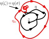
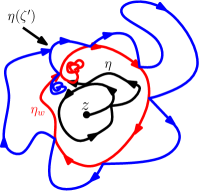
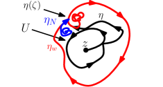

Suppose that is a GFF flow line and that is an almost surely finite stopping time for such that . We say that the outer boundary of can be represented as the tail of a flow line if the following is true. Let be the largest time before that (note ). Then there exists with rational coordinates which is contained in a bounded complementary component of such that is contained in a tail of the flow line starting at . See Figure 3.12 for an illustration. The main ingredient in our proof of the existence of a decomposition of a flow line into overlapping tails is the following lemma, which says that if the outer boundary of is represented as a tail, then the outer boundary of is almost surely represented by a tail where is the first time after that wraps around its starting point and intersects itself. One example of such a stopping time is the first time after a fixed time that makes a clean loop about . We will establish this through repeated applications of Lemma 3.11.
Lemma 3.12.
Let be a whole-plane GFF defined up to a global multiple of and let be the flow line of starting at . Let be any almost surely finite stopping time for such that the outer boundary of can be represented as a tail of a flow line, as described just above. Let be the first time that . Then the outer boundary of is almost surely represented as a tail of a flow line.
Proof.
Let be as described just before the statement of the lemma and let be the flow line of starting at whose tail covers the outer boundary of (see Figure 3.12). Let be a bounded connected component of whose boundary contains and is traced by for some small with (see Figure 3.13 for an illustration). Let be a sequence in with rational coordinates which converges to and, for each , let be the flow line of starting from . Let be first integer such that cleanly merges into . Then Lemma 3.11 implies that almost surely. It follows from Proposition 3.5 that merges into and does not separate from , at least up until both paths reach (this is when the starting point of at least one of the two tails is separated from ). Consequently, also merges with and the two paths agree with each other, at least up until they both hit .
Let be the first time that hits and let be the first time after that wraps around and hits itself. We are now going to argue that agrees with up to reparameterization (see Figure 3.14 for an illustration of the argument). To see this, we will first argue that is almost surely contained in the unbounded connected component of . Let be the start and end times of the tail of which represents the outer boundary of . Since cleanly merges into , we know that the height difference of at and , as made precise in Figure 1.13, is either (if is a clockwise loop, as in Figure 3.14, heights go down by ) or (if is a counterclockwise loop, heights go up by ). Consequently, it follows by applying Proposition 3.5 to and stopped at a time before merges into that does not cross (see Remark 3.13 below). This proves our claim. The proof that is equal to follows since boundary emanating flow lines are almost surely determined by the field [MS16d, Theorem 1.2] and absolute continuity [MS16d, Proposition 3.4]. This is explained in more detail in the caption of Figure 3.14. ∎
Remark 3.13.
Although the starting point of is random and depends on the realization of (or ) in the proof of Lemma 3.12 above, we can still apply Proposition 3.5. The reason is that the starting points of and were assumed to be rational and Proposition 3.5 describes almost surely the interaction of all tails of flow lines started at rational points simultaneously. Consequently, we do not have to worry about the dependencies in the definitions of the flow lines in order to determine the manner in which their tails interact upon hitting.
Proof of Proposition 3.6.
The result follows by repeatedly applying the previous lemma to get that each time wraps around and hits itself, it can be represented by a tail. ∎
Proof of Proposition 3.7.
It is easy to see from the proof of Proposition 3.5 that it generalizes to describe the interaction of a tail of a flow line of starting from an interior point of and a tail of (which we recall starts from ). (Depending on the boundary data of , it may be can intersect itself. This, for example, is the case in the setting of Figure 3.3.) Let be the first time that intersects itself. Consequently, it is easy to see from Lemma 3.9 as well as the argument used to prove Lemma 3.11 that can be decomposed into a union of overlapping tails starting at points with rational coordinates. That the same holds for follows from the argument used to prove Proposition 3.6. ∎
3.2.3 Flow line interaction
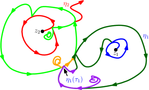
Proposition 3.6 allows us to extend the observations from Proposition 3.5 from tails to entire flow lines, since wherever two flow lines intersect (or one flow line intersects its past), locally it can be described by two flow line tails starting from points with rational coordinates intersecting.
Proof of Theorem 1.7 for ordinary GFF flow lines.
In the case that , we know from Section 2.1.3 and Lemma 2.4 that flow lines of the GFF are non-self intersecting hence are themselves tails. Consequently, in this case the result follows from Proposition 3.5 as well as absolute continuity if is a proper subdomain in (Proposition 2.16). This leaves us to handle the case that which is in turn explained in the caption of Figure 3.15. We emphasize that it is important that all of the tails considered in the proof have initial points with rational coordinates so that we can use Proposition 3.5 to describe the interaction of all of these tails simultaneously almost surely. The result for boundary emanating flow lines follows by a similar argument and Proposition 3.7. ∎
We will explain in Section 3.3 after completing the proof of the existence component of Theorem 1.4 how using absolute continuity, the version of Theorem 1.7 for ordinary GFF flow lines implies Theorem 1.7 as stated, in particular in the presence of a conical singularity.
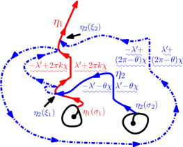
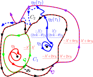
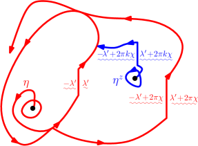
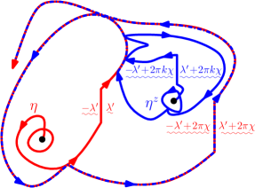
Now that we have proved Theorem 1.7 for ordinary GFF flow lines, we turn to prove Theorem 1.9 for ordinary GFF flow lines ().
Proposition 3.14.
Suppose that is a domain, is a GFF on defined up to a global multiple of if , , and . For , let be the flow line of with angle , i.e. the flow line of , starting from . Then and almost surely cross each other at most once. If , then almost surely do not cross.
Proof.
We first suppose that are distinct. The first step in the proof is to show that tails of ordinary GFF flow lines can cross each other at most once. This is explained in the caption of Figure 3.16. Since ordinary GFF flow lines are themselves tails when , to complete the proof we just need to handle the case that . The proof of this is explained in the caption of Figure 3.17. This completes the proof in the case that are distinct. Now suppose that . We can run, say , up until an almost surely positive stopping time so that . Then the same arguments imply that almost surely crosses at most once. Since the stopping time was arbitrary, it follows that and almost surely cross at most once. In the case that , a trivial scaling argument implies that and almost surely do not cross. That almost surely do not cross in the case that follows from the case and absolute continuity. ∎
Proposition 3.15.
Suppose that is a whole-plane GFF defined up to a global multiple of and that are flow lines of starting at distinct with the same angle. Then and almost surely merge.
Proof.
We first consider the case that . Since whole-plane processes are almost surely unbounded, it follows from Lemma 2.6 that almost surely surrounds and separates from . Let be the (necessarily bounded) connected component of which contains . Theorem 1.7 implies that cannot cross , hence can exit only upon merging with (see also Figure 3.19 and Figure 3.20). Since is also almost surely unbounded, exits almost surely, from which the result in this case follows. When , does not intersect itself so the argument we gave for does not apply directly. The appropriate modification is explained in the caption of Figure 3.18. One aspect of the proof which is not explained in the caption is why the connected components of are almost surely bounded. The reason is that the conditional law of given and for and indices taken mod is that of an process with and such processes almost surely swallow any fixed point in finite time. ∎
Remark 3.16.
Suppose that we are in the setting of Proposition 3.15 with replaced by a GFF on a proper subdomain in . Then it is not necessarily true that and merge with probability one. The reason is that, depending on the boundary data, there is the possibility that and get stuck in the boundary (i.e., intersect the boundary with a height difference which does not allow the curve to bounce off the boundary) before intersecting each other with the appropriate height difference.
Remark 3.17.
Assume that we are in the setting of Proposition 3.15 with so that almost surely surrounds , except that has angle for and . By Theorem 1.7, once hits , it either crosses immediately or bounces off . Just as in the case that , as in Figure 3.19 and Figure 3.20, it might be that has to wind around several times before ultimately leaving the complementary connected component (“pocket”) of which contains . Note that the pockets of are ordered according to the order in which traces their boundary and, after leaving the pocket which contains , passes through the pockets of according to this ordering.
3.3 Conical singularities
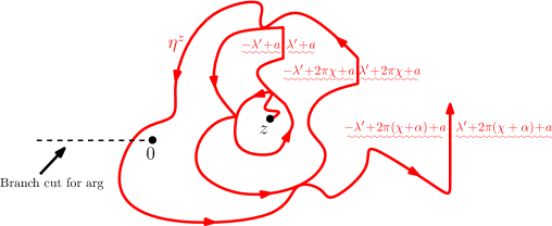
Let be a whole-plane GFF. In this section, we are going to construct a coupling between , viewed as a distribution up to a global multiple of , and a whole-plane process where , provided (so that ). This will complete the proof of the existence part of Theorem 1.4. In Section 3.4, we will establish the uniqueness component of Theorem 1.4. Recall from Remark 3.3 that the proof of Theorem 1.1 goes through without modification in order to prove the existence of the coupling when and . Thus we just need to extend the proof of Theorem 1.1 in order to get the result for , which is stated and proved just below.
Proposition 3.18.
Fix constants , , and suppose that viewed as a distribution defined up to a global multiple of where is a whole-plane GFF. There exists a unique coupling where is an process with
| (3.8) |
such that the following is true. For every -stopping time , the conditional law of given is given by a GFF on with -flow line boundary conditions (as in Figure 1.10) on , a gap along viewed as a distribution defined up to a global multiple of , and the same boundary behavior at as .
Proof.
We are going to give the proof when for simplicity since, just as in the proof of Theorem 1.1 as explained in Remark 3.3, the case for general follows from the same argument. We consider the same setup used to prove Theorem 1.1 described in Section 3.1: we let , be a GFF on such that has the boundary data as indicated in the left side of Figure 3.3. More concretely, this means that the boundary data for is near on the left side of , near on the right side of , and changes by times the winding of the boundary otherwise.
By [MS16d, Theorem 1.1, Theorem 1.2, and Proposition 3.4], we know that there exists a well-defined flow line of starting from (i.e., a coupling which satisfies the desired Markov property). Let where, as in the proof of Theorem 1.1, . Then is equal in law to where is a GFF on with the boundary data as indicated in the right side of Figure 3.3 and is equal to the harmonic extension of from to . As before, the branch cut of is on the half-infinite line from through . It follows from [MS16d, Proposition 3.4] and Proposition 3.1 that there exists a unique coupling of with a continuous process (equal in law to ) whose law is mutually absolutely continuous with respect to that of a radial process in targeted at with a single boundary force point at , up until any finite time when parameterized by -conformal radius as viewed from , such that the coupling satisfies the Markov property described in the statement of Proposition 3.1. To complete the proof of the proposition, we just need to determine the law of . We are going to accomplish this by computing the Radon-Nikodym derivative of the law of with respect to the law of where for each . Note that is a radial process in targeted at with a single force point located at .
We begin by computing the Radon-Nikodym derivative of the law of with respect to the law of away from . For each and such that , we let denote the average of about (see [DS11, Section 3] for a discussion of the construction and properties of the circle average process). Let
and be the annulus centered at with in-radius and out-radius . Note that . The Radon-Nikodym derivative of the law of with respect to is proportional to
| (3.9) |
This is in turn proportional to since (see the end of the proof of [DS11, Proposition 3.1]; the reason for the difference in sign is that the function in [DS11] is times the function used here).
Let . Since is parameterized by -conformal radius as viewed from , by the Koebe- theorem [Law05, Corollary 3.18] we know that for all . By [DS11, Proposition 3.2] and the Markov property for the GFF, we know that the law of given for is equal to the sum of and a mean-zero Gaussian random variable with variance . Moreover, and are independent. By combining this with (3.9), it thus follows that
| (3.10) |
(note that this makes sense as a Radon-Nikodym derivative between laws on paths because is determined by ). The reason that we know that we have the correct normalization constant is that it follows from [MS16d, Proposition 6.5] that evolves as a standard Brownian motion in .
Let be the driving pair for . In this case, . By the Girsanov theorem [KS91, RY99], to complete the proof we just need to calculate the cross-variation of and the Brownian motion which drives . By conformally mapping and applying (1.2) (see Figure 3.1), we see that we can represent explicitly in terms of and . Let . Note that (resp. ) is equal to the harmonic measure of the counterclockwise segment of from to (resp. to ). We have that
The integral in the first equality represents the contribution to the conditional mean from the winding terms in the boundary data. This corresponds to integrating times the harmonic extension of the winding of to . Since we are evaluating the harmonic extension at , this is the same as computing the mean of times the winding of . Finally, the reason that the term appears is due to the coordinate change formula (1.2). (Note that if then the boundary data is immediately to the left of and immediately to the right. Here, when we write we are taking the branch of with values in where the branch cut is on . In particular, .)
Recall the form (2.5) of the SDE for . We thus see that the cross-variation of and is given by . Since the Brownian motion which drives is the same as that which drives , we therefore have that the driving pair of solves the SDE (2.4) with where the driving Brownian motion is replaced with . In other words, solves (2.4) with , as desired. ∎
Now that we have established the existence component of Theorem 1.4, we can complete the proof of Theorem 1.7.
Proof of Theorem 1.7.
In Section 3.2, we established Theorem 1.7 for ordinary GFF flow lines. Since the law of away from is mutually absolutely continuous with respect to the law of the ordinary field on the same domain and GFF flow lines are local (i.e., a flow line started at a point in an open set stopped upon exiting depends only on the field in ), the interaction result for flow lines of follows from the interaction result for the ordinary GFF. ∎
Remark 3.19.
If we are given where is a GFF on a domain and we want to speak of “the flow line started at with angle ” then, in order to decide how to get the flow line started, we have to know (or at least its restriction to a neighborhood of ) modulo an additive multiple of . We also have to choose a branch of the argument function defined on a neighborhood of (or, alternatively, to define the argument on the universal cover of and to let represent a fixed element of that universal cover). However, once these two things are done, there is no problem in uniquely defining the flow line of angle beginning at .
In order to define a flow line started from the origin of a fixed angle with , it is necessary to know modulo a global additive multiple of , at least in a neighborhood of . We can simultaneously draw a flow line from both an interior point and from if we know the distribution both modulo a global additive multiple and modulo a global additive multiple of . This is possible, for example, if is a bounded domain, and we know precisely (not up to additive constant). It is also possible if and the field is known modulo a global additive multiple of some constant which is an integer multiple of both and .
Remark 3.20.
If we say that is a flow line of starting from , then we mean it is either generated in the sense of Remark 3.19 if we know the the field up to a global multiple of or in the sense of Remark 3.20 otherwise. We end this subsection with the following, which combined with Proposition 3.14 completes the proof of Theorem 1.9.
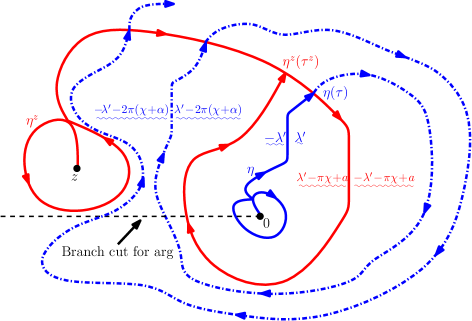
Proposition 3.21.
Fix constants , , suppose that is a domain, is a GFF on , and . When , assume that is defined modulo a global multiple of . Fix . Let be flow lines of starting from (resp. ). Assume that has zero angle. In the case that , we assume that we either know up to a global multiple of or that has a random angle; see Remark 3.19 and Remark 3.20. There exists a constant such that and almost surely cross each other at most times. Moreover, almost surely can cross itself at most the same constant times ( does not cross itself).
Lemma 3.22.
Suppose that and . Let be an process in from to with force points located at . Then the Lebesgue measure of is almost surely zero.
Lemma 3.23.
Suppose that is an process with and in from to with a single boundary force point located at . Let be the first time that hits . Then the law of has a density with respect to Lebesgue measure on .
Proof.
For each , let be the event that has not swallowed by time . On , we let be the unique conformal map which sends to and fixes both and . Fix . It is clear from the form of the driving function for chordal that, on , has a density with respect to Lebesgue measure. Consequently, the same is likewise true for (since for is smooth on ). Let be the time that first hits . Let be an independent copy of and let be the first time that it hits . For a Borel set , we have that
This implies that, on , the law of has a density with respect to Lebesgue measure. Since as , it follows that in fact has a density with respect to Lebesgue measure. ∎
Lemma 3.24.
Suppose that is a GFF on with piecewise constant boundary data. Let be the flow line of starting from and let be the first time that hits . Fix any open interval on which the boundary data for is constant. Assume that the probability of the event that exits in is positive. Conditional , the law of has a density with respect to Lebesgue measure on .
Proof.
This follows from Lemma 3.23 and absolute continuity. ∎
Lemma 3.25.
Suppose that we have the same setup as Proposition 3.21. Fix and let be the component of which contains . Then the harmonic measure of the self-intersection points of which are contained in as seen from is almost surely zero.
Proof.
Proof of Proposition 3.21.
The beginning of the proof in the case that is explained in the caption of Figure 3.22. We are left to bound the number of times that can cross (using the notation of the figure). Let and let be the times at which crosses . For each , let be the height difference of the paths when crosses at time . Assume (as is illustrated in Figure 3.22) that hits at time on its right side. We are going to show by induction that, for each for which , that
-
(i)
crosses from the right to the left of at time ,
-
(ii)
almost surely does not hit a self-intersection point of at time , and
-
(iii)
the height difference of the paths upon crossing at this time satisfies
(3.11)
Here, we take so that (iii) holds automatically for . That (ii) holds for follows from Lemma 3.24 and Lemma 3.25. Finally, (i) holds by assumption. Upon completing the proof of the induction, Theorem 1.7 implies that for each , so (3.11) implies that the largest for which is at most .
Suppose that and that (i)–(iii) hold for all . We will show that (i)–(iii) hold for . Let be the first time that hits so that forms a loop around . That (ii) holds for implies that there exists a complementary pocket of and such that . Let (resp. ) be the first (resp. second) segment of which is traced by . Theorem 1.7 implies that cannot cross (this is the side of that crossed into at time ). Therefore can exit only through or through the terminal point of , i.e., the last point on drawn by .
Note that is coupled with the conditional GFF given starting from as a flow line. (Theorem 1.7 implies that the conditional mean of given drawn up to any stopping time before exiting and has flow line boundary conditions on and the arguments of [MS16d, Section 6] imply that has a continuous Loewner driving function viewed as a path in .) In particular, the conditional law of given is that of an process. Thus, in the case that crosses out of , that (ii) holds for follows from Lemma 3.22, Lemma 3.25, and absolute continuity. In this case, it is also immediate from the setup that (i) and (iii) hold for (it is topologically impossible for the path to cross out of through from the left to the right). It is not difficult to see that if does not cross out of , i.e., exits at the last point on drawn by , then it does not subsequently cross . ∎
3.4 Flow lines are determined by the field
We are now going to prove Theorem 1.2, that in the coupling of Theorem 1.1, is almost surely determined by , as well as the corresponding statement from Theorem 1.4. (We will also complete our proof of the uniqueness of the law of the coupling in the case of flow lines started from interior points associated with a GFF on a proper subdomain of .) This is the interior flow line analog of the uniqueness statement for boundary emanating flow lines from [MS16d, Theorem 1.2]. As we will explain just below, the result is a consequence of the following proposition. We remind the reader of Remark 3.4.
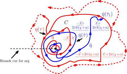
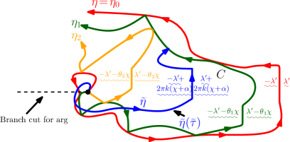
Proposition 3.26.
Fix constants , , and let , viewed as a distribution defined up to a global multiple of , where is a whole-plane GFF. Suppose that , are coupled with as flow lines starting from the origin as in the statement of Theorem 1.1 () or Theorem 1.4 () such that given , and are conditionally independent. Then almost surely.
Before we prove the proposition, we record the following simple lemma.
Lemma 3.27.
Fix constants , , and let , viewed as a distribution defined up to a global multiple of , where is a whole-plane GFF. Fix angles and let be the flow lines of with angles starting from taken to be conditionally independent given . Then and almost surely do not cross. Likewise, if and is the flow line of the conditioned field given with angle , then and almost surely do not cross.
Proof.
We know from Proposition 3.21 that and cross each other at most a finite number of times. Let be the distance to of the last crossing of and . We take if does not cross . By the scale invariance of the coupling , it follows that almost surely, which proves the first assertion of the lemma. The second assertion is proved similarly. (In particular, the argument of Proposition 3.21 implies that and can cross each other at most the same constant times.) ∎
Proof of Proposition 3.26.
Recall that if then and are distributed as whole-plane processes with . Thus the paths are self-intersecting in this case when (so that ) and are simple if (so that ). Moreover, for these are the same ranges of in which the paths are either self-intersecting or simple, respectively. Indeed, these assertions follow from Lemma 2.4. We will handle the two cases separately.
We first suppose that we are in the self-intersecting regime. Suppose that is a stopping time for the filtration such that is not contained in the range of ; on the event , we take . It is explained in Figure 3.23 that, on , almost surely merges into and does not separate from , say at time . Let be the modulus of the point where first merges into . Then what we have shown implies that is finite almost surely. The scale invariance of the coupling implies that the law of is also scale invariant, hence almost surely. Therefore .
We now suppose that we are in the regime of in which the paths are simple. We condition on and fix evenly spaced angles such that the following is true. Let be the flow line of the conditional GFF on given starting at with angle . We assume that the angles have been chosen so that almost surely intersects both and where the indices are taken mod and (by [MS16d, Theorem 1.5] we know that we can arrange this to be the case — see also Figure 3.18 as well as Section 2.3). Again by the scale invariance of the coupling , it suffices as in the case that paths are self-intersecting to show that almost surely merges with . The argument is given in the caption of Figure 3.24. We remark that the reason that we took the flow lines in Figure 3.24 to be for the conditional field given is that we have not yet shown that the rays of the field started at the same point with varying angle are monotonic. ∎
Proof of Theorem 1.2 and Theorem 1.4.
Proposition 3.26 implies Theorem 1.2 and the uniqueness statement of Theorem 1.4 in the case that the domain of the GFF is given by the whole-plane . Thus to complete the proofs of these results, we just need to handle the setting that is a proper subdomain of . This, however, follows from absolute continuity (Proposition 2.16). ∎
Proof of Theorem 1.1 and Theorem 1.4, uniqueness for general domains.
We will first give the proof in the case that and . Suppose that is a GFF on a general domain and that is a path coupled with with the property that for each -stopping time we have that is a local set for and the conditional law of given is that of a GFF on with flow line boundary conditions on . We assume without loss of generality that the starting point of is equal to . Suppose that is a flow line of starting from whose law is induced from the whole-plane measure on flow lines as in the proof of Theorem 1.1. Then we know that the law of is, by construction, absolutely continuous with respect to that of a whole-plane , at least up until the first time that it hits the ball of radius . As , it therefore follows that for each the number of components that separates from before hitting is infinite almost surely. We know that the flow line interaction result applies to , . In particular, can cross at most once and if intersects with a height difference of then the two paths merge and do not subsequently separate. If stopped upon hitting has not yet merged with then it would be forced to cross an infinite number of times before hitting . This is a contradiction and therefore must merge with before hitting . Since this holds for all , we conclude that and coincide up until hitting . The flow line interaction result implies that the two paths cannot separate after hitting and therefore agree for all time.
The case that and is proved in a similar manner except one uses a collection of flow lines starting from with equally spaced angles, all induced from the whole-plane measure, in place of as in the proof of Proposition 3.26 given above.
The case for general values of is handled similarly. ∎
The proof that the boundary emanating flow lines of the GFF are uniquely determined by the field established in [Dub09b] and extended in [MS16d] is based on duality (a flow line can be realized as the outer boundary of a certain counterflow line). There is also an duality based approach to establishing the uniqueness of flow lines started at interior points which will be a consequence of the material in Section 4.2. The duality approach to establishing these uniqueness results also gives an alternative proof of the merging phenomenon and the boundary emanating version of this is discussed in [MS16d, Section 7].
Proof of Theorem 1.8.
The statement that is a local set for is a consequence of [MS16d, Proposition 6.2] and Theorem 1.2. Consequently, the statement regarding the conditional law of given follows since we know the conditional law of given and Proposition 2.15. The final statement of the theorem follows [MS16d, Theorem 1.2]. ∎
Theorem 1.4 implies that we can simultaneously construct the entire family of rays of the GFF starting from a countable, dense set of points each with the same angle as a deterministic function of the underlying field. We will now prove Theorem 1.10, that the family of rays in fact determine the field.
Proof of Theorem 1.10.
Let be a countable, dense set of and fix . For each , let be the flow line of starting from with angle . For each , let be the -algebra generated by . Fix and recall that denotes the inner product of and . We are going to complete the proof of the theorem by showing that
| (3.12) |
By the martingale convergence theorem, the limit on the left side of (3.12) exists almost surely. Consequently, to prove (3.12), it in turn suffices to show that
| (3.13) |
For each , let denote the Green’s function of . We note that makes sense for each since almost surely has harmonically non-trivial boundary. Moreover, we have that for each fixed distinct and (this can be seen from the stochastic representation of ). Let be a compact set which contains the support of and let . Since
and is integrable on , by the dominated convergence theorem it suffices to show that for each fixed distinct. This follows from the Beurling estimate [Law05, Theorem 3.69] (by the stochastic representation of ) since there exists a subsequence of with . This proves (3.13), hence the theorem. ∎
Theorem 1.4 also implies that we can simultaneously construct the entire family of rays of the GFF starting from any single point (resp. the location of the conical singularity) if (resp. ) with varying angles as a deterministic functional of the underlying field, that is, the family of flow lines of for . We are now going to show that the rays are monotonic in their angle as well as compute the conditional law of one such path given another. This is in analogy with [MS16d, Theorem 1.5] for flow lines emanating from interior points.
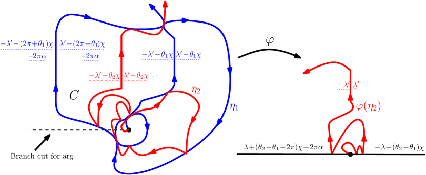
Proposition 3.28.
Fix constants , , and angles with . Let be a whole-plane GFF and , viewed as a distribution defined up to a global multiple of . For , let be the flow line of starting from with angle . Then almost surely does not cross (though may bounce off) . In particular, if is self-intersecting, then visits the components of according to their natural ordering (the order that their boundaries are drawn by ). Moreover, the conditional law of given is independently that of a chordal process in each of the components of with
If with and is the flow line of starting from with angle , then the conditional law of given and is independently that of a chordal process in each of the components of with
Proof.
The first assertion of the proposition, that and almost surely do not cross, is a consequence of Lemma 3.27. The remainder of the proof is explained in the caption of Figure 3.25, except for three points. First, we know that the conditional mean of given and up to any fixed pair of stopping times does not exhibit singularities at their intersection points by Theorem 1.7. Secondly, that viewed as a path in complementary connected component of has a continuous Loewner driving function. This follows from the arguments of [MS16d, Section 6.2]. Thirdly, the reason that intersects on its right side with a height difference of (as illustrated in Figure 3.25) rather than for some is that this would lead to the paths crossing, contradicting Lemma 3.27. The result then follows by invoking [MS16d, Theorem 2.4 and Proposition 6.5]. The proof of the final assertion follows from an analogous argument. ∎
Proposition 3.28 gives the conditional law of one GFF flow line given another, both started at a common point. We will study in Section 5 the extent to which this resampling property characterizes their joint law. We also remark that it is possible to state and prove (using the same argument) an analog of Proposition 3.28 which holds for GFF flow lines on a bounded domain, though it is slightly more complicated to describe the conditional law of one path given the other because one may have to deal with force points on the outer boundary. (Moreover, when a path hits the boundary, it is sometimes possible to “branch” the path in two different directions and the way that this is to be done has to be specified.) We recall that some additional discussion about what can happen when single path hits the boundary appears in Section 3.2.3 (which includes the proof of Theorem 1.7).
3.5 Transience and endpoint continuity
Suppose that is a whole-plane GFF, , and . Let be the flow line of , viewed as a distribution defined up to a global multiple of , starting from . In this section, we are going to prove that is transient, i.e. almost surely. This is equivalent to proving the transience of whole-plane processes for , , and . This in turn completes the proof of Theorem 1.12 for ; we will give the proof for in Section 4. Using the relationship between whole-plane and radial processes described in Section 2.1, this is equivalent to proving the so-called “endpoint continuity” of radial for , , and . This means that if is a radial process in and targeted at then almost surely. This was first proved by Lawler in [Law11] for ordinary radial processes and the result we prove here extends this to general processes, though the method of proof is different. The main ingredient in the proof of this is the following lemma.
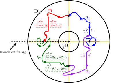
Lemma 3.29.
Let be a GFF on , , , and let , viewed as a distribution defined up to a global multiple of . Let . There exists depending only on , , and such that the following is true. Let be the event that there exists an angle varying flow line of which
-
(i)
Starts from a point with rational coordinates,
-
(ii)
Changes angles only upon hitting the straight lines with angles starting from for ,
-
(iii)
Travels with angles contained in ,
-
(iv)
Stops upon exiting the annulus , , and
-
(v)
Disconnects from .
Then .
Proof.
It is proved in the caption of Figure 3.26 that the event that there exists an angle varying flow line starting from with the properties described in the lemma statement for satisfies . Consequently, the result follows by scale invariance. We explain further a few points here. First, the reason for our choice of is that it implies that the angle changes as defined in the figure caption are contained in . This is important because there is only a range of angles at which we can draw flow lines from a given point in . Second, the reason that we have to construct an angle varying flow line is that, for some values of , it is not possible for a flow line to hit itself after wrapping around . Moreover, the reason that it is necessary to have multiple angle changes (as opposed to possibly just one), depending on the value of , is that with each angle change we can only change the boundary height adjacent to the path by at most in absolute value while the height of a single path changes by in absolute value upon winding once around . ∎
Proposition 3.30.
Suppose that is a whole-plane process for , , and starting at . Then almost surely. Moreover, if is a radial process in and targeted at for , , and , then almost surely.
Proof.
From the relationship between whole-plane and radial described in Section 2.1.3, the two assertions of the proposition are equivalent. Fix , , a whole-plane GFF, and let , viewed as a distribution defined up to a global multiple of . Let be the flow line of starting from . Then it suffices to show that almost surely. Let and let be the event as described in the statement of Lemma 3.29 for the annulus and the corresponding angle-varying flow. On , it follows that because Proposition 3.21 implies that can cross each of the angle-varying flow lines hence a finite number of times and we know that almost surely (the capacity of the hull of is unbounded as ). Thus it suffices to show that, almost surely, infinitely many of the events occur. This follows from the following two observations. First, the Markov property implies that is independent of conditional on . Moreover, the total variation distance between the law of conditional on and the law of (unconditional) converges to zero almost surely as (see Section 2.2.2). Therefore the claim follows from Lemma 3.29. ∎
3.6 Critical angle and self-intersections
The height gap divided by is called the critical angle . Recalling the identities and (see (2.9)–(2.11)), we see that the critical angle can be written
| (3.14) |
Note that , , , , and more generally
| (3.15) |
Recall from Figure 2.3 that in the boundary emanating setting, is the critical angle at which flow lines can intersect each other. In the setting of interior flow lines, has the same interpretation as a consequence of Theorem 1.7 and Theorem 1.11. Moreover, gives the maximum number of distinct ordinary GFF flow lines emanating from a single interior point that one can start which are non-intersecting. In particular, is the critical value for which an interior flow line does not intersect itself (recall also that for , we have as well as Lemma 2.4). The value of which solves is critical for being able to fit distinct non-intersecting interior GFF flow lines starting from a single point. Explicitly, this value of is given by
| (3.16) |
If we draw distinct non-intersecting interior flow lines, starting at a common point, with angles evenly spaced on the circle , then these flow lines will intersect each other if and only if . The value of which solves is critical for a single flow line being able to visit the same point times (wrapping around the starting point of the path once between each visit — so that the angle gap between the first and last visit is ). This allows us to determine whether a flow line almost surely has triple points, quadruple points, etc. We record this formally in Proposition 3.31 below.
If we consider flow lines of , viewed as a distribution defined up to a global multiple of , where is a whole-plane GFF, , and as in Theorem 1.4, the value of which is critical for a flow line starting at to be able to intersect itself is the non-negative solution to . Note that this in particular depends on but not and that as decreases to , the critical value of decreases to . Similarly, the value of which solves is critical for the intersection of flow lines whose angles differ by .
Proposition 3.31.
Suppose that where is a whole-plane GFF, , and , viewed as a distribution defined up to a global multiple of and let be the flow line of starting from . Almost surely, the maximal number of times that hits any single point is (i.e., the maximal multiplicity)
| (3.17) |
Equivalently, almost surely, the maximal number of times that a whole-plane or radial process for , , and hits any single point is given by
| (3.18) |
Finally, almost surely, the maximal number of times that a radial process for , , and can hit any point on the domain boundary (other than its starting point) is given by
| (3.19) |
Proof.
In between each successive time that hits any given point, it must wrap around its starting point. Consequently, when hits a given point for the th time, it intersects itself with a height difference of . That is, the intersection can be represented as the intersection of two flow line tails which intersect each other with the aforementioned height difference. Theorem 1.7 implies that from which (3.17) and (3.18) follow. A similar argument gives (3.19). ∎
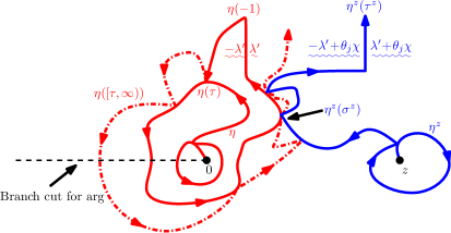
The following proposition will be used in [MW17] to compute the almost sure Hausdorff dimension of the set of points that hits exactly times. Let denote the Hausdorff dimension of a set .
Proposition 3.32.
Suppose that we have the same setup as Proposition 3.31. For each , let be the set of points that hits exactly times and
| (3.20) |
Assume that, for each , there exists a constant such that
| (3.21) |
where are flow lines of a GFF on starting from with an angle difference of such that the event conditioned on in (3.21) occurs with positive probability. Then
We emphasize that the assumption (3.21) in the statement of Proposition 3.32 applies to any choice of boundary data for the GFF on and starting points for . That is, the angle difference determines the almost sure dimension of the intersection points which are contained in (the interior of) and nothing else. (The dimension of for , however, does depend on the boundary data for .) The value of for is computed in [MW17]. The value of is the dimension of ordinary chordal : [Bef08]. Note that when , is equal to the critical angle (3.14) and exceeds the critical angle for larger values of .
Proof of Proposition 3.32.
The set of points that hits exactly times can be covered by the set of intersections of pairs of flow line tails starting from points with rational coordinates which intersect with an angle gap of . By the proofs of Proposition 3.5 and Proposition 3.6, the law of the dimension of each of these intersections is absolutely continuous with respect to the intersection of two boundary emanating GFF flow lines with an angle gap of . This proves the upper bound.
We are now going to give the proof of the lower bound. See Figure 3.27 for an illustration. Assume that is between and the (common) values in (3.17), (3.18) (for or values of which exceed (3.17), (3.18), there is nothing to prove). Assume that is parameterized by capacity. For each , let be the set of points that hits exactly times by time and which are not contained in the boundary of the unbounded connected component of . By the conformal Markov property of whole-plane , it suffices to show that there exists such that
| (3.22) |
To see that this is the case, we let be the first time after time that makes a clean loop around and condition on . Lemma 2.6 implies that occurs with positive probability. Let . By [Law05, Proposition 3.27], is contained in the unbounded component of on . On , let be the flow line of starting from with angle . (The reason we are able to set the angle for is that, after fixing an infinitesimal segment of , we know the remainder of the field up to a multiple of ; see Remark 3.19.) Let be the first time hits . Lemma 3.9 implies that the event that hits at time with an angle difference of occurs with positive conditional probability given . Let be a stopping time for given which is strictly larger than such that, on , we have that and only intersect with an angle difference of . To finish the proof of (3.22), it suffices to show that contains given with positive conditional probability. Iteratively applying Lemma 3.9 implies that, each of the first times that wraps around , it has a positive chance of hitting (hence itself) and, moreover, this occurs before (capacity) time for . After wrapping around times, by Lemma 2.6, has a positive chance of making a clean a loop before intersecting itself again or time . Theorem 1.7 then implies that, on these events, the set of points that hits in by the time it has wrapped around times contains . This implies the desired result. ∎
Proposition 3.33.
Fix , , and let where is a GFF on such that has the boundary data as illustrated in Figure 3.1. Let be the flow line of starting from and assume that either or . For each , let be the set of points in that hits exactly times. Assume that, for each , there exists a constant such that
| (3.23) |
where is the flow line of a GFF on starting from whose boundary data is such that almost surely intersects with an angle difference of . Then
provided .
Note that Proposition 3.33 gives the dimension of the set of points that radial , and , hits the boundary times.
4 Light cone duality and space-filling SLE
4.1 Defining branching processes

As usual, we fix and . Consider a GFF on with piecewise constant boundary conditions (and only finitely many pieces). Recall that if the boundary conditions are constant and equal to on the negative real axis and constant and equal to on the positive real axis, by [MS16d, Theorem 1.1] one can draw a counterflow line from to whose law is that of ordinary , as in Figure 4.1. For each , let (resp. ) be the flow line of starting from with angle (resp. ). In this section, we will argue that the left and right boundaries of an initial segment of the counterflow line are in some sense described by and where is the tip of that segment, as illustrated in Figure 4.1. When and the counterflow line is space-filling, we can describe and beginning at any point as the boundaries of a counterflow line stopped at the first time it hits . We will show in this section that when it is still possible to construct a “branching” variant of that has a branch that terminates at (and the law of this branch is the same as that of a certain radial process targeted at ). The flow lines and will then be the left and right boundaries of this branch, just as in the case . We will make sense of this construction for both boundary and interior points . (When is an interior point, we will have to lift the branch to the universal cover of in order to define its left and right boundaries.)

We begin by constructing (for a certain range of boundary conditions) a counterflow line of that “branches” at boundary points. Recall that we can draw a counterflow line from to provided that the boundary data is piecewise constant (with only finitely many pieces) and strictly greater than on the negative real axis and strictly less than on the positive real axis [MS16d, Section 7]. (This is a generalization of the construction in Figure 4.1.) Given this type of boundary data, the continuation threshold almost surely will not be reached before the path reaches . Indeed, it was shown in [MS16d, Section 7] that if these constraints are satisfied then the counterflow line is almost surely continuous and almost surely tends to as (capacity) time tends to .
Now suppose we consider a real point and try to draw a path targeted at . By conformally mapping to , we find that we avoid reaching the continuation threshold at a point on if each boundary value on that interval plus is strictly greater than (recall (1.2) and see Figure 4.2). That is, the values on are strictly greater than . We can draw a counterflow line from to every point if the boundary values on the positive real axis are in the interval . Similarly, we can draw a counterflow line from to every point if the boundary values on the negative real axis are in the interval . We can draw the counterflow line to each fixed point in if the boundary function is given by which is piecewise constant, takes on only a finite number of values, and satisfies
| (4.1) |
(In the case of an process, this corresponds to each being in the interval .) When these conditions hold, we say that the boundary data is fully branchable, and we extend this definition to general domains via the coordinate change (1.2) (see also Figure 1.7). The reason we use this term is as follows.
If we consider distinct , then the path targeted at will agree with the path targeted at (up to time parameterization) until , the first time that either one of the two points is hit or the two points are “separated,” i.e., lie on the boundaries of different components of . Indeed, this follows because both paths (up until separating and ) are coupled with the field as described in [MS16d, Theorem 1.1] and [MS16d, Theorem 1.2] implies that there is a unique such path coupled with the field, so they must agree. The two paths evolve independently after time , so as explained in Figure 4.3 we can interpret the pair of paths as a single path that “branches” at time (with one of the branches being degenerate if a point is hit at time ). We can apply the same interpretation when and are replaced by a set . In that case, a branching occurs whenever two points are separated from each other for the first time. At such a time, the number of distinct components containing at least one of the increases by one, so there will be branching times altogether. If the boundary conditions are fully branchable, then we may fix a countable dense collection of , and consider the collection of all counterflow lines targeted at all of these points. We refer to the entire collection as a boundary-branching counterflow line. Note that if we have constant boundary conditions on the left and right boundaries, so that the counterflow line targeted at is an process, then we can extend the path toward every provided that for .
Similarly, we may consider a point in the interior of , and the (fully branchable) boundary conditions ensure that we may draw a radial counterflow line from targeted at which almost surely reaches before hitting the continuation threshold. The branching construction can be extended to this setting, as explained in Figure 4.4. By considering a collection of counterflow lines targeted at a countable dense collection of such , we obtain what we call an interior-branching counterflow line. This is a sort of space-filling tree whose branches are counterflow lines. When the values of on are given by either
-
(i)
on and on or
-
(ii)
on and on ,
then this corresponds to the exploration tree rooted at the origin introduced in [She09]. The boundary conditions in (i) correspond to having the force point lie to the left of and the boundary conditions in (ii) correspond to having the force point lie to the right of .
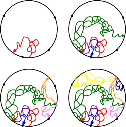
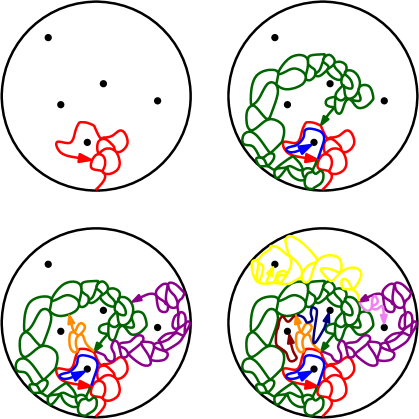
4.2 Duality and light cones
Figure 4.5 is lifted from [MS16d, Section 7], which contains a general theorem about the boundaries of chordal processes. Suppose that is a Jordan domain. The theorem states that if the boundary conditions on are such that a counterflow line can almost surely be drawn from to a point without hitting the continuation threshold, then the left and right boundaries of the counterflow line are respectively the flow lines of angle and drawn from to (with the caveat that these flow lines may trace part of the boundary of the domain toward if they reach the continuation threshold before reaching , as Figure 4.5 illustrates — this corresponds to the scenario in which the counterflow line fills an entire boundary arc, as explained in [MS16d, Section 7]). We will not repeat the full discussion of [MS16d, Section 7] here, but we will explain how it can be extended to the setting where the boundary target is replaced with an interior point. (In this setting can be understood as a branch of the interior-branching counterflow line, as discussed in the previous section.) This is the content of Theorem 4.1.
Theorem 4.1.
Suppose that is a Jordan domain, are distinct, and that is a GFF on whose boundary conditions are such that its counterflow line from to is fully branchable. Fix and let be the counterflow line of starting from and targeted at . If we lift to a path in the universal cover of , then its left and right boundaries and are the flow lines of started at and targeted at with angles and , respectively (with the same caveat as described above, and in [MS16d, Section 7], in the chordal case: that these paths may trace boundary segments toward if they hit the continuation threshold before reaching ). The conditional law of given and in each of the connected components of which are between , consist of boundary segments of that do not trace , and are hit by is independently that of a chordal process starting from the last point on the component boundary traced by and targeted at the first.
Remark 4.2.
Suppose that is a connected component of which lies between and part of whose boundary is drawn by a segment of either or which does trace part of . Then it is also possible to compute the conditional law of given and inside of . It is that of an process where the weights depend on the boundary data of on the segments of which trace .
Remark 4.3.
Since is almost surely determined by the GFF [MS16d, Theorem 1.2] (see also [Dub09b]), this gives us a different way to construct and . In fact, taking a branching counterflow line gives us a way to construct simultaneously all of the flow lines beginning at points in a fixed countable dense subset of . It follows from [MS16d, Theorem 1.2] that the branching counterflow line is almost surely determined by the GFF, so this also gives an alternative approach to proving Theorem 1.2, that GFF flow lines starting from interior points are almost surely determined by the field.
Remark 4.4.
Both and can be projected to itself (from the universal cover) and interpreted as random subsets of . Once we condition on and , the conditional law of within each component of (that does not contain an interval of on its boundary) is given by an independent (boundary-filling) chordal curve from the first to the last endpoint of within that component. This is explained in more detail in the beginning of [MS16f] and the end of [MS16d], albeit in a slightly different context. It follows from this and the arguments in [MS16d] that we can interpret the set of points in the range of as a light cone beginning at . Roughly speaking, this means that the range of is equal to the set of points reachable by starting at and following angle-varying flow lines whose angles all belong to the width- interval of angles that lie between the angles of and . The analogous statement that applies when is contained in the boundary is explained in detail in [MS16d]. We refrain from a more detailed discussion here, because the present context is only slightly different.
Remark 4.5.
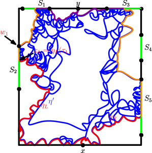
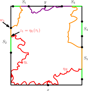
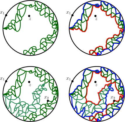
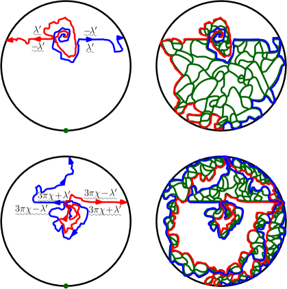
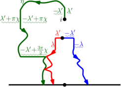
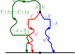
Proof of Theorem 4.1.
The result essentially follows from the chordal duality in [MS16d, Section 7.4.3] (which the reader may wish to consult before reading the argument here) together with the merging arguments of Section 3.4 (such as the proof of Proposition 3.15). The argument is sketched in Figure 4.6, which extends Figure 4.5 to the case of an interior point. It is somewhat cumbersome to repeat all of the arguments of [MS16d, Section 7.4.3] here, so we instead give a brief sketch of the necessary modifications. We inductively define points as follows. We let be the unique conformal map with and and then take . We then let be the first time for which fails to lie on the boundary of the connected component of containing . Given that the stopping time has been defined for , let be the unique conformal map which takes the connected component of which contains to with and . We then take and let be the first time that fails to lie on the boundary of the component of containing . It is easy to see that there exists constants and such that the probability that the conformal radius of (as viewed from ) is at most times the conformal radius of (as viewed from ) is at least . By basic distortion estimates (e.g., [Law05, Theorem 3.21]), one can make the analogous statement for the ordinary radius (e.g., ). This implies that the concatenated sequence of counterflow line path segments illustrated in Figure 4.6 contains as a limit point.
For each , it follows from [MS16d, Theorem 1.4] that the left and right boundaries of (where we take ) are contained in the flow lines and with angles and , respectively, of the conditional GFF given for starting from . That is, we a priori have to observe for in order to draw the aforementioned flow lines. We are going to show by induction on that the left and right boundaries of are contained in the union of all of the flow lines of itself with angles and , respectively, starting at points with rational coordinates. (In other words, it is not necessary to observe for to draw these paths.) This, in turn, will allow us to use Theorem 1.7 to determine how the left and right boundaries of interact with the flow lines of . The claim for follows from [MS16d, Theorem 1.4].
Suppose that the claim holds for some fixed . Fix , with rational coordinates, and let be the flow line starting from with angle . Theorem 1.7 determines the manner in which interacts with the flow lines of both itself as well as those of given for , at least up until the paths hit . Therefore it follows from the arguments of Lemma 3.11 that the segments of are contained in the union of flow lines of starting from rational coordinates with angle . If and merges with , then after hitting and bouncing off , both paths will continue to agree. The reason is that both paths reflect off in the same direction and satisfy the same conformal Markov property viewed as flow lines of the GFF given for as well as the segments of and drawn up until first hitting . See the proof of Lemma 3.12 for a similar argument. Consequently, the entire range of is contained in the union of flow lines of with angle starting from points with rational coordinates. The same likewise holds with and in place of and . This proves the claim.
We will now show that and give the left and right boundaries of . Suppose that . In this case, makes loops around since the path is not space-filling. Suppose that is a stopping time for at which it has made a clockwise loop around . Theorem 1.7 (recall Figure 3.19 and Figure 3.20) then implies that almost surely merges into the left boundary of before leaving the closure of the component of which contains . The same likewise holds when we replace with and is a stopping time at which has made a counterclockwise loop. The result follows because, as we mentioned earlier, almost surely tends to and, by (the argument of) Lemma 2.6, almost surely makes arbitrarily small loops around with both orientations. The argument for so that does not make loops around is explained in Figure 4.8.
It is left to prove the statement regarding the conditional law of given and . Since the left and right boundaries of are given by and , respectively, it follows that is almost surely equal to the concatenation of the counterflow lines of the conditional GFF given and in each of the components of which are visited by . Indeed, the restriction of to each of these components satisfies the same conformal Markov property as each of the corresponding counterflow lines of the conditional GFF. Thus, the claim follows from [MS16d, Theorem 1.2]. By reading off the boundary data of in each of these components, we see that if such a component does not intersect in an interval, then the conditional law of is independently that of an , as desired. ∎
We now extend Theorem 4.1 to the setting in which we add a conical singularity to the GFF.
Theorem 4.6.
The statements of Theorem 4.1 hold if we replace the GFF with and where is a GFF on such that the counterflow line of starting from is fully branchable.
Remark 4.7.
The value is significant because it is the critical value for at which fills its own outer boundary. That is, if then fills its own outer boundary and if then does not fill its own outer boundary. This corresponds to a value of (recall Figure 3.2).
Remark 4.8.
If and the boundary data of is given by (resp. ) on (resp. ), then is a radial process where (recall Figure 3.2).
Proof of Theorem 4.6.
The argument is the same as the proof of Theorem 4.6. In particular, we break the proof into the two cases where
-
1.
so that can hit its own outer boundary as it wraps around and
-
2.
so that cannot hit its own outer boundary as it wraps around .
The proof in the first case is analogous to the proof of Theorem 4.1 for and the second is analogous to Theorem 4.1 with . Note that for , almost surely. ∎
Proof of Theorem 1.6 and Theorem 1.15.
Assume that , viewed as a distribution modulo a global multiple of , is defined on all of . The construction of the coupling as described in Theorem 1.6 follows from the same argument used to construct the coupling in Theorem 1.1 and Theorem 1.4; see Remark 3.3. The statement of Theorem 1.15 follows due to the way that the coupling is generated as well as Theorem 4.1 and Theorem 4.6. Finally, that the path is almost surely determined by follows because Theorem 1.2 and Theorem 1.4 tell us that its left and right boundaries and , respectively, are almost surely determined by . Moreover, once we condition on and , we know that is coupled with independently as a chordal counterflow line in each of the components of which are visited by . This allows us to invoke the boundary emanating uniqueness theory [MS16d, Theorem 1.2]. The case that follows by absolute continuity (Proposition 2.16). The other assertions of Theorem 1.15 follow similarly. ∎
Proof of Theorem 1.12.
We finish this subsection by computing the maximal number of times that a counterflow line can hit a given point or the domain boundary and then relate the dimension of the various types of self-intersection points of counterflow lines to the dimension of the intersection of GFF flow lines starting from the boundary.
Proposition 4.9.
Fix and . Suppose that is a GFF on and , viewed as a distribution defined up to a global multiple of . Let be the counterflow line of starting from . Let
The maximal number of times that can hit any given point (i.e., maximal multiplicity) is given by
| (4.2) |
In particular, the maximal number of times that a radial or whole-plane process with and can hit any given point is given by
| (4.3) |
Finally, the maximal number of times that a radial process with and process can hit the domain boundary is given by
| (4.4) |
The value in the statement of Proposition 4.9 gives the maximal number of times that a chordal or process can hit an interior point. In particular, chordal and processes have double but not triple points or higher order self-intersections for and have triple points but not higher order self-intersections for . The other expressions in the maximum function in (4.2), (4.3) give the number of intersections which can arise from the path winding around its target point and then hitting itself. In particular, note that the first expression in the maximum in (4.3) is identically equal to for , i.e. is at least the critical value for such a process to have this type of self-intersection (Lemma 2.4). Similarly, the first expression in the maximum in (4.4) vanishes for .
Proof of Proposition 4.9.
As we explained before the proof, there are two sources of self-intersections in the interior of the domain:
-
1.
The double () and triple () points which arise from the segments of restricted to each of the complementary components of the left and right boundaries of that it visits, and
-
2.
The intersections of the left and right boundaries of .
Since chordal is a boundary-filling, continuous process, it is easy to see that the set of double or triple points of the first type mentioned above which are also contained in the left and right boundaries of is countable. (If is in the left or right boundary of , is the first time that hits and is the second, then the interval must contain a rational.) Consequently, the two-self intersection sets are almost surely disjoint as . Moreover, we note that the self-intersections which are contained in the left and right boundaries arise by the path either making a series of clockwise or counterclockwise loops. In such successive loops, the points that hits times correspond to the points where the left (resp. right) side of hits the right (resp. left) side times. Theorem 1.15 then tells us that the height difference of the aforementioned intersection set is given by . Then (4.2), (4.4) follow by solving for the value of that makes this equal to and applying Theorem 1.7.
We will now prove (4.4). For concreteness, we will assume that is a radial process in starting from with a single boundary force point of weight located at , i.e. immediately to the left of . We can think of as the counterflow line of where is a GFF on so that the sum has the boundary data illustrated in Figure 3.2. Then wraps around and hits a boundary point for the th time for with either a height difference of (if the first intersection occurs to the left of the force point) or with a height difference of otherwise (see Figure 3.2). (The reason that we now have in place of as in the previous paragraph is because here we have added rather than subtracted it.) Solving for the value of that makes this equal to and then applying Theorem 1.7 yields the first two expressions in the maximum. The final expression in the maximum comes from the multiple boundary intersections that can occur when the process interacts with the boundary before passing through the force point (as well as handles the possibility that the process can only hit the boundary one time after passing through the force point). ∎
Proposition 4.10.
Suppose that we have the same setup as in Proposition 4.9 and assume that the assumption (3.21) of Proposition 3.32 holds. For each , let be the set of interior points that hits exactly times which are contained in the left and right boundaries of and let
| (4.5) |
Then
where is the dimension of the intersection of boundary emanating GFF flow lines with an angle gap of .
Note that the angle in (4.5) is equal to the critical angle (3.14) when and and exceeds the critical angle for larger values of .
Proof of Proposition 4.10.
Proposition 4.11.
Fix and . Suppose that where is a GFF on so that has the boundary data depicted in Figure 3.2 with (i.e., is immediately to the left of ). Let be the counterflow line of starting from so that with . Assume that assumption (3.23) of Proposition 3.33 holds. Let (resp. ) be the set of points that hits on exactly times where the first intersection occurs to the left (resp. right) of the force point. For each , let
For each , we have
where is the dimension of the intersection of a boundary emanating flow line in with where the path hits with an angle gap of .
4.3 Space-filling
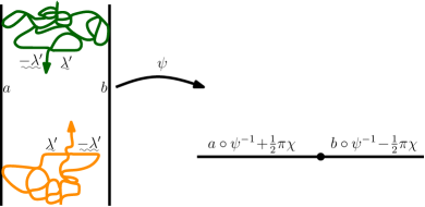
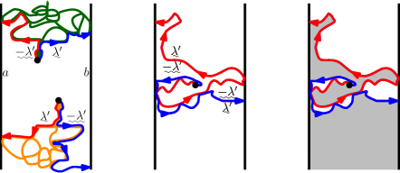
In this section, we will prove the existence and continuity of the space-filling processes for , thus proving Theorem 1.16. Recall that these processes are defined in terms of an induced ordering on a dense set as described in Section 1.2.3; see also Figure 1.16 as well as Figure 4.9 and Figure 4.10. As we will explain momentarily, Theorem 1.19 follows immediately from Theorem 1.16 since the definition of space-filling has time-reversal symmetry built in. Theorem 1.19 in turn implies Theorem 1.18. For the convenience of the reader, we restate these results in the following theorem. We remind the reader that the range of values considered in Theorem 4.12 is summarized in Figure 1.18 and Figure 1.19.
Theorem 4.12.
Let be a Jordan domain and fix distinct. Suppose that and and let be a GFF on whose counterflow line from to is an process (which is fully branchable). Then space-filling in from to exists, is well-defined, and almost surely is a continuous path when parameterized by area. The path is almost surely determined by and the path almost surely determines . When and , space-filling describes the same law as chordal . Moreover, the time-reversal of a space-filling is a space-filling in from to where is the reflection of about the line. In particular, space-filling has time-reversal symmetry.
Proof of Theorem 1.17.
Fix . Suppose that is a GFF on a Jordan domain such that its counterflow line growing from a point is an process with a single force point located at . Then the branching counterflow line of starting from targeted at a countable dense set of interior points describes the same coupling of radial processes used to generate the exploration tree in rooted at [She09]. It follows from the construction of space-filling that the branch of targeted at a given interior point agrees with the space-filling process coupled with starting from parameterized by conformal radius as seen from . Consequently, the result follows from the continuity of space-filling proved in Theorem 4.12. Indeed, if was not almost surely locally finite, then there would exist such that the probability that there are an infinite number of loops with diameter at least is positive. Since the space-filling process traces the boundary of each of these loops in a disjoint time interval, it would follow that there would be an infinite number of pairwise disjoint time intervals whose image under the space-filling have diameter at least . Since the total area of the domain was assumed to be finite and space-filling is parameterized by area, it follows that the interval of time on which it is defined is finite. Therefore there must exist a sequence in such that the length of the intervals tends to as . This contradicts the almost sure continuity of space-filling , which proves the result. ∎
Remark 4.13.
One can extend the definition of the space-filling processes to the setting of many boundary force points. These processes make sense and are defined in the same way provided the underlying GFF has fully branchable boundary data. Moreover, there are analogous continuity and reversibility results, though we will not establish these here. The former can be proved by generalizing our treatment of the two force point case given below using arguments which are very similar to those used to establish the almost sure continuity of the chordal processes in [MS16d, Section 7] and the reversibility statement is immediate from the definition once continuity has been proved. In this more general setting, the time-reversal of a space-filling process is a space-filling process where the vectors of weights are chosen so that, for each and , is the reflection of about the line where .
We remind the reader that the range of values considered in Theorem 4.12 is summarized in Figure 1.18 and Figure 1.19. We will now explain how to derive the time-reversal component of Theorem 4.12 (see also Figure 1.16 as well as Figure 4.9 and Figure 4.10). Consider a GFF on a vertical strip in and assume that the boundary value function for is piecewise constant (with finitely many discontinuities) and satisfies
| (4.6) |
These boundary conditions ensure that we can draw a counterflow line from the bottom to the top of as well as from the top to the bottom, as illustrated in Figure 4.9. In each case the counterflow line is an process where for with . When the boundary conditions are equal to a constant (resp. ) on the left (resp. right) side of , the counterflow line starting from the bottom of the strip is an process with
| (4.7) |
(see Figure 4.9). In this case, the restriction (4.6) is equivalent to . The counterflow line from the top to the bottom of is an where
| (4.8) |
That is, for is the reflection of about the line and . These boundary conditions are fully branchable and both the counterflow line of the field from the top to the bottom and for the counterflow line of the field from the bottom to the top of hit both sides of . We note that the order in which the two counterflow lines hit points is as described in Figure 1.16. Moreover, (4.7) and (4.8) together imply that Theorem 1.19 follows once we prove Theorem 1.16.
What remains to be shown is the almost sure continuity of space-filling and that the process is well-defined (i.e., the resulting curve does not depend on the choice of countable dense set). Recall that the ordering which defines space-filling was described in Section 1.2.3; see also Figure 1.16 as well as Figure 4.9 and Figure 4.10. By applying a conformal transformation, we may assume without loss of generality that we are working on a bounded Jordan domain . We then fix a countable dense set of (where we take ) and, for each , let (resp. ) be the flow line of starting from with angle (resp. ). For distinct indices , we say that comes before if lies in a connected component of part of whose boundary is traced by either the right side of or the left side of . For each , the sets divide into pockets . For each , consists of those points in connected components of part of whose boundary is traced by a non-trivial segment of either the right side of or the left side of (see Figure 4.10 for an illustration) before either path merges into some or for and consists of those points in . For each , let denote the index of the th point in in the induced order. We then take to be the piecewise linear path connecting where the amount of time it takes to travel from to is equal to the area of . Let be the diameter of . Then to prove that the approximations to space-filling are almost surely Cauchy with respect to the metric of uniform convergence of paths on the interval whose length is equal to the area of , it suffices to show that
| (4.9) |
Moreover, this implies that the limiting curve is well-defined because if is another countable dense set and is the sequence with and then it is clear from (4.9) that the limiting curve associated with is the same as the corresponding curve for both and .
For each and , we let denote the diameter of stopped at the first time that it either merges with one of for with or hits with the appropriate height difference (as described in Figure 4.10). We let (resp. ) denote the diameter of the counterclockwise (resp. clockwise) segment of starting from towards that stops the first time it hits one of the (resp. ) for at a point where the path terminates in . Finally, we define and analogously except starting from with the former segment traveling in the clockwise direction and the latter counterclockwise direction. Then it follows that
| (4.10) |
Consequently, to prove (4.9) it suffices to show that the right side of (4.10) almost surely converges to as . We are going to prove this by first showing that an analog of this statement holds in the setting of the whole-plane (Proposition 4.14 in Section 4.3.1) and then use a series of conditioning arguments to transfer our whole-plane statements to the setting of a bounded Jordan domain. This approach is similar in spirit to our proof of the almost sure continuity of chordal processes given in [MS16d, Section 7] and is carried out in Section 4.3.2. As we mentioned in Remark 4.13, this approach can be extended to establish the almost sure continuity of the many-force-point space-filling processes by reusing more ideas from [MS16d, Section 7], though we will not provide a treatment here.
4.3.1 Pocket diameter estimates in the whole-plane
Let be a whole-plane GFF viewed as a distribution defined up to a global multiple of . We will now work towards proving an analog of the statement that the right side of (4.10) converges to as which holds for the flow lines of started in a fine grid of points. Specifically, we fix and let be the grid of points in which are entirely contained in . For each , let be the flow line of starting from . Fix ; we will eventually take to be large (though not changing with ). Fix and let . For each and , let be the first time that leaves . Note that if . Let .
Proposition 4.14.
There exists constants and such that for every and with the following is true. The probability that does not merge with any of for is at most .
For each , we let be a point such that (where we break ties according to some fixed but unspecified convention). Let , i.e., half of the critical angle. By Theorem 1.7, a flow line with angle almost surely hits a flow line of zero angle started at the same point on its left side. For each , let be the flow line of starting from with angle and let be the first time that leaves . Let be the -algebra generated by as well as for . Let be the event that separates from and that the harmonic measure of the left side of as seen from in the connected component of which contains is at least . See Figure 4.11 for an illustration of the setup as well as the event . We will make use of the following lemma in order to show that it is exponentially unlikely that fewer than a linear number of the events occur for .
Lemma 4.15.
Fix and . Suppose that is a GFF on with boundary data so that its flow line starting from is an process with and force points located at . Fix such that the flow line of starting from with angle almost surely does not hit the continuation threshold and almost surely intersects . Let (resp. ) be the first time that (resp. ) leaves . Let be the event that separates from and that the harmonic measure of the left side of as seen from in is at least . There exists depending only on , , , and (but not and ) such that .
Proof.
That for a fixed choice of follows from the analogies of Lemma 3.8 and Lemma 3.9 which are applicable for boundary emanating flow lines. That is uniformly positive for all and follows since the law of an process is continuous in the location of its force points [MS16d, Section 2]. When either or , we can use absolute continuity to compare to the case that either , , or both. Indeed, suppose for example that and . Let be the function which is harmonic in and whose boundary values are given by
Then is a GFF on whose boundary values are (resp. ) on (resp. ) so that its flow line starting from is an ordinary process. Moreover, if with and then is uniformly bounded in and and the flow line of stopped upon exiting is equal to the corresponding flow line of . Therefore the claim that we get a uniform lower bound on as and vary follows from [MS16d, Remark 3.5]. The other possibilities follow from a similar argument. ∎
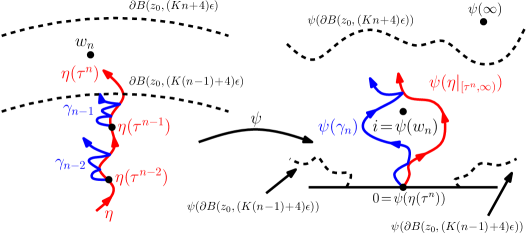
Lemma 4.16.
There exists constants and such that for every and we have
Proof.
Let be the conformal map which takes the unbounded connected component of to with and . The Beurling estimate [Law05, Theorem 3.69] and the conformal invariance of Brownian motion together imply that if we take sufficiently large then the images of and under lie outside of . Consequently, the law of restricted to is mutually absolutely continuous with respect to the law of a GFF on restricted to whose boundary data is chosen so that its flow line starting from is a chordal process with a single force point located at the image under of the most recent intersection of with itself (or just a chordal process if there is no such self-intersection point which lies in ). The result then follows from Lemma 4.15 (and the argument at the end of the proof of Lemma 4.15 implies that we get a lower bound which is uniform in the location of the images ). ∎
On , let be the event that merges with upon exiting . Let .
Lemma 4.17.
There exists and such that for every and we have
Proof.
Proof of Proposition 4.14.
Assume that has been chosen sufficiently large so that Lemma 4.16 and Lemma 4.17 both apply. Lemma 4.16 implies that it is exponentially unlikely that we have fewer than of the events occur and Lemma 4.17 implies that it is exponentially unlikely that we have fewer than a fraction of these in which occurs. ∎
4.3.2 Conditioning arguments
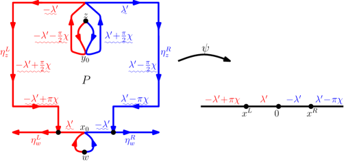
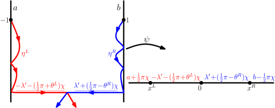
In this section, we will reduce the continuity of space-filling processes to the statement given in Proposition 4.14 thus completing the proof of Theorem 4.12. The first step is the following lemma.
Lemma 4.18.
Suppose that is a whole-plane GFF viewed as a distribution defined up to a global multiple of . Fix distinct. Let (resp. ) be the flow line of starting from with angle (resp. ) and define analogously. Then the probability that the pocket formed by these flow lines (as described in Figure 4.12) is contained in is positive.
Proof.
Proof of Theorem 4.12.
We are going to prove the almost sure continuity of space-filling in three steps. In particular, we will first establish the result for , then extend to the case that , and then finally extend to the most general case that .
Step 1. . Let be a whole-plane GFF viewed as a distribution defined up to a global multiple of . Fix distinct and let be the pocket formed by the flow lines of with angles and starting from , as described in Lemma 4.18 (the particular choice is not important). Let be a conformal map which takes to with the opening (resp. closing) point of taken to (resp. ). Note that is a GFF on whose boundary data is such that its counterflow line starting from is an process with force points located at the images of the points where and merge; see Figure 4.11. Note that (resp. ) is contained in the clockwise (resp. counterclockwise) segment of from to .
Proposition 4.14 and a union bound implies that the following is true. The maximal diameter of those flow lines started in with angles and stopped upon merging with a flow line of the same angle started in goes to zero almost surely as . Consequently, conditionally on the positive probability event that , the maximal diameter of the pockets formed by the flow lines with angles and starting from the points in tends to zero with (conditional) probability one. Indeed, this follows because we have shown that the right side of (4.10) tends to zero with (conditional) probability one. This implies that there exists (resp. ) in the clockwise (resp. counterclockwise) segment of from to and a countable, dense set of such that space-filling in from to with force points located at generated from flow lines starting at points in is almost surely continuous. Once we have shown the continuity for one fixed choice of countable dense set, it follows for all countable dense sets by the merging arguments of Section 3. (Recall, in particular, Lemma 3.11.) Moreover, we can in fact take and by further conditioning on the flow lines of starting from and with angle and , respectively, which are reflected towards and then restricting the path to the complementary component which contains ; see also Figure 4.13. (Equivalently, in the setting of Figure 4.12, we can reflect the flow lines and towards the opening point of the pocket .)
Step 2. . Suppose that is a GFF on as in Figure 4.13 where we take the boundary conditions to be and . By (4.7), is compatible with a coupling with a space-filling process from to . Let (resp. ) be the flow line of starting from (resp. ) with angle (resp. ). Note that as , converges to the half-infinite vertical line starting starting from to and that when , “merges” with the right side of . The angles and have analogous interpretations for . Let be the unbounded connected component of whose boundary contains and let be a conformal map which takes the first intersection point of and to and sends to . Then is a space-filling process in (recall Remark 4.13) where
Moreover, the force points associated with and are immediately to the left and to the right of the initial point of the path. For each , let . Fix . Since the law of restricted to converges in total variation as to the law of a GFF on whose boundary conditions are compatible with a coupling with space-filling process, also restricted to , we get the almost sure continuity of the latter process stopped the first time it exits . By adjusting the angles and , we can take to be any pair of values in . This proves the almost sure continuity of space-filling for from to in stopped upon exiting for each . To complete the proof of this step, we just need to show that if is a space-filling process with then is almost surely transient: that is, almost surely. This can be seen by observing that, almost surely, infinitely many of the flow line pairs starting from for with angles and stay inside of the annulus (the range of after hitting is almost surely contained in the closure of the unbounded connected component of ). Indeed, this follows from Lemma 3.9 and that the total variation distance between the law of given and that of (unconditionally) converges to zero when is fixed and . (See the proof of Lemma 3.29 for a similar argument.)
Step 3. . By time-reversal, Step 2 implies the almost sure continuity of space-filling where is the reflection of about the line. In particular, we have the almost sure continuity of space-filling for all . We are now going to complete the proof by repeating the argument of Step 2. Fix . Suppose that is a GFF on whose boundary conditions are chosen so that the associated space-filling process from to satisfies for . Explicitly, this means that the boundary data for is equal to some constant (resp. ) on the left (resp. right) side of with
We let (resp. ) be the flow line of starting from (resp. ) with angle (resp. ). The range of angles is such that the flow line (resp. ) is almost surely defined and terminates upon hitting the right (resp. left) side of or . In particular, neither path tends to . The conditional law of the space-filling process associated with in the unbounded connected component of with on its boundary is a space-filling process with
In particular, when (resp. ) takes on its minimal (resp. maximal) value, (resp. ). When (resp. ) takes on its maximal (resp. minimal) value, (resp. ). By adjusting and (as in Step 2), we can arrange it so that and . The proof is completed by using the scaling and transience argument at the end of Step 2. ∎
5 Whole-plane time-reversal symmetries
In this section we will prove Theorem 1.20. The proof is based on related arguments that appeared in [MS16e, Section 4]. In [MS16e, Section 4], the authors considered a pair of chordal flow lines and in a domain . The starting and ending points for the are the same but the paths have different angles. It was observed that when is given, the conditional law of is that of a certain type of process in the appropriate component of . A similar statement holds with the roles of and reversed. It is proved in [MS16e] that these conditional laws (of one given the other) actually determine the overall joint law of the pair . We will derive Theorem 1.20 as a consequence of the following analog of the result from [MS16e, Section 4]. (Note that the first half is just a restatement of Theorem 1.11 and Theorem 1.12. The uniqueness statement in the final sentence is the new part.)
Theorem 5.1.
Suppose that is a whole-plane GFF, , , and let , viewed as a distribution defined up to a global multiple of . Fix . Let (resp. ) be the flow line of with angle (resp. ) starting from . Let be the joint law of the pair defined in this way. The pair has the following properties:
-
(i)
Almost surely, and have liftings to the universal cover of that are simple curves which do not cross each other (though, depending on and , they may intersect each other). Moreover, almost surely neither curve traces the other (i.e., neither curve intersects the other for any entire open interval of time).
-
(ii)
The are transient: almost surely.
-
(iii)
Given , the conditional law of the portion of intersecting each component of is given by an independent chordal process in (starting at the first point of hit by and ending at the last point of hit by ) with
(5.1) A symmetric statement holds with the roles of and reversed.
Every probability measure on path pairs satisfying (i)–(iii) can be expressed uniquely as
| (5.2) |
where is a probability measure on .
As we will explain in Section 5.3, Theorem 1.20 is almost an immediate consequence of Theorem 5.1. The goal of the rest of this section is to prove Theorem 5.1. The most obvious approach would be as follows: imagine that we fix some given initial pair . Then “resample” from the conditional law given . Then “resample” from its conditional law given . Repeat this procedure indefinitely, and show that regardless of the initial values of , the law of the pair of paths after resamplings “mixes”, i.e., converges to some stationary distribution, as .
And indeed, the proof of the analogous result in [MS16e, Section 4] is based on this idea. Through a series of arguments, it was shown to be sufficient to consider the mixing problem in a slightly modified context in which the endpoints of were near to but distinct from the endpoints of . The crucial step in solving the modified mixing problem was to show that if we consider an arbitrary initial pair and a distinct pair , then we can always couple together the resampling procedures so that after a finite number of resamplings, there is a positive probability that the two pairs are the same.
In this section, we will extend the bi-chordal mixing arguments from [MS16e, Section 4] to a whole-plane setting. In the whole-plane setting, we consider a pair of flow lines from to in of different angles of , viewed as a distribution defined up to a global multiple of , starting from the origin with given values of and , as described in Theorem 5.1. We will show that these paths are characterized (up to the term) by the nature of the conditional law of one of the given the other (in addition to some mild technical assumptions). Since this form of the conditional law of one path given the other has time-reversal symmetry (i.e., is symmetric under a conformal inversion of that swaps and ), this characterization will imply that the joint law of has time-reversal symmetry. (The fact that this characterization implies time-reversal symmetry was already observed in [MS16e].)
The reader who has not done so will probably want to read (or at least look over) [MS16e, Section 4] before reading this section. Some of the bi-chordal mixing arguments in [MS16e, Section 4] carry through to the current setting with little modification. However, there are some topological complications arising from the fact that paths can wind around and hit themselves and each other in complicated ways. Section 5.1 will derive the topological results needed to push through the arguments in [MS16e]. Also, [MS16e, Section 4] is able to reduce the problem to a situation in which the starting and ending points of and are distinct — the reduction involves first fixing and up to some stopping time and then fixing a segment of a counterflow line starting from the terminal point, so that and exit at different places. This is a little more complicated in the current setting, because drawing a counterflow line from infinity may not be possible in the usual sense (if the angle is too small) and one has to keep track of the effect of the height changes after successive windings around the origin, due to the argument singularity. Section 5.2 will provide an alternative construction that works in this setting.
The constructions and figures in this section may seem complicated, but they should be understood as our attempt to give the simplest (or at least one reasonably simple) answer to the following question: “What modifications are necessary and natural for extending the methods of [MS16e, Section 4] to the context of Theorem 5.1?”
5.1 Untangling path ensembles in an annulus
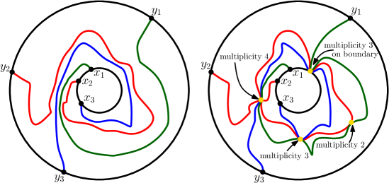
In order to get the mixing argument to work, we need to show that the relevant space of paths is in some sense connected. The difficulty which is present in the setting we consider here in contrast to that of [MS16e, Section 4] is the paths may wrap around the origin and intersect themselves and each other many times.
Fix a closed annulus with distinct points (ordered counterclockwise) in the interior annulus boundary and distinct points (ordered counterclockwise) on the exterior annulus boundary and an integer . Define an -tangle (as illustrated in Figure 5.1) to be a collection of distinct continuous curves in such that
-
1.
Each starts at and ends at .
-
2.
The lifting of each to the universal cover of is a simple curve (i.e., a continuous path that does not intersect itself).
-
3.
The (necessarily closed) set of times for which intersects another curve (or intersects its own past/future) is a set with empty interior and no crosses itself or any distinct .
-
4.
The lifting of to the universal cover of winds around the interior annulus boundary a net times (rounded down to the nearest integer). This fixes a homotopy class for (and by extension for all of the ).
-
5.
Every has multiplicity at most , where the multiplicity of is the number of pairs for which .
-
6.
Each has multiplicity at most and no path hits one of the endpoints of another path.
Let be the graph whose vertex set is the set of all -tangles and in which two -tangles and are adjacent if and only if for some we have
-
1.
(up to monotone reparameterization) for all
-
2.
There is one component of
and a pair of times (after monotone reparameterization if necessary) such that , , and and agree outside of .
Lemma 5.2.
The graph is connected. In other words, we can get from any -tangle to any other -tangle by finitely many steps in .
Proof.
We will first argue that regardless of the value of , we can get from any -tangle to some -tangle in finitely many steps. We refer to the connected components of as pockets and observe that for topological reasons the boundary of each pocket is comprised of at most two path segments (and perhaps parts of the boundary of ). The (at most two) endpoints of the pocket are those points common to these two segments. Boundary points of a pocket that are not endpoints are called interior boundary points of the pocket.
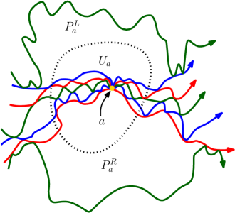
For every multiplicity point , we can find a small neighborhood of whose pre-image in consists of disjoint open intervals. The images of these segments in are simple path segments that do not cross each other, and that all come together at . The leftmost such segment is part of the right boundary of a single pocket and the rightmost such segment is part of the left boundary of a single pocket , as illustrated in Figure 5.2.
We now claim that at most finitely many pockets have a multiplicity- boundary point that is not one of the two endpoints of the pocket. If there were infinitely many such pockets, then (by compactness of ) we could find a sequence of corresponding multiplicity points (each a non-endpoint boundary of a different pocket) converging to a point . Clearly has multiplicity at least so it must be an interior point in and we can construct the neighborhood containing as described above; but the only two pockets within this neighborhood that can have interior multiplicity- boundary points are the pockets and , as illustrated in Figure 5.2. Since only two pockets intersecting have multiplicity- interior boundary points, there cannot be an infinite sequence of such pockets intersecting and converging to , so we have established a contradiction and verified the claim.
Now, within each pocket, we can move the left or right boundary away (getting rid of all multiplicity points on its boundary) in single step without introducing any new multiplicity points. Repeating this for each of the pockets with multiplicity boundary points allows us to remove all multiplicity points in finitely many steps.
A similar procedure allows us to remove any multiplicity boundary points from the boundary of . (A multiplicity boundary point on is essentially a multiplicity boundary point if we interpret a boundary arc of as one of the paths. Every such point is on the interior boundary of exactly one pocket and the same argument as above shows that there are only finitely pockets with interior.)
We have now shown that we can move from any -tangle to an -tangle in finitely many steps. Repeating this procedure allows us to get to a -tangle in finitely many steps. In a -tangle all of the paths are disjoint and they intersect only at their endpoints. For the remainder of the proof, it suffices to show that one can get from any -tangle to any other -tangle with finitely many steps in . It is easy to see that one can continuously deform to since the two are homotopically equivalent. Similarly one can continuously deform all of in such a way that gets deformed to and the other paths get mapped to continuous paths. One can then fix the first path and deform the domain to take the second path to , and so forth. Ultimately we obtain a continuous deformation of to within the space of -tangles. By compactness, the minimal distance that one path gets from another during this deformation is greater than some . We can now write the continuous deformation as a finite sequence of steps such that each path moves by at most (in Hausdorff distance) during each step. Thus we can move the paths one at a time through these steps without their interfering with each other. Repeating this for each step, we can get from to with finitely many moves in . ∎
5.2 Bi-chordal annulus mixing
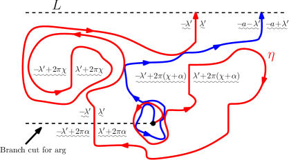
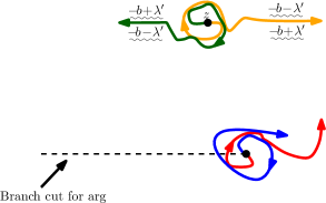
In this section, we will complete the proof of Theorem 5.1. Throughout, we shall assume that are paths satisfying (i)–(iii) of Theorem 5.1. In order to get the argument of [MS16e, Section 4] to work, we will need to condition on an initial segment of each of and as well as some additional paths which start far from . This conditioning serves to separate the initial and terminal points of and . The idea is to imagine that are coupled with an ambient GFF on . We then pick some point which is far away from zero and draw flow lines , of starting from where the angle of is chosen uniformly from (recall Remark 1.5) and points in the opposite direction of , i.e. the angle of is relative to that of (see Figure 5.4). Conditioning on and as well as initial segments of and then puts us into the setting of Section 5.1.
We cannot carry this out directly because a priori (assuming only the setup of the second part of Theorem 5.1) we do not have a coupling of with a GFF on . We circumvent this difficulty as follows. Conditioned on the pair , we let be an instance of the GFF on . We let have -flow line boundary conditions on and where the value of and the angles on each are determined so that if were flow lines of a GFF with an singularity and these angles then they would have the same resampling property, as in the statement of Theorem 5.1. (Note that as in (5.1) determine and .)
We then use the GFF to determine the law of , at least until one hits or . As in Figure 5.7, we would ultimately like to continue and all the way to . We accomplish this by following the rule that when one of the hits one of the , it either reflects off or immediately crosses , depending on what it would do if were in fact a GFF flow line hit at the same angle (as described in Theorem 1.7). To describe the construction more precisely, we will first need the following lemma which serves to rule out the possibility that hits one of the at a self-intersection point of or at a point in .
Lemma 5.3.
Suppose that is a pocket of . Then the harmonic measure of each of the sets
-
(i)
the self-intersection of points of each ,
-
(ii)
as seen from any point in is almost surely zero.
Proof.
This follows from the resampling property and Lemma 3.22. Indeed, fix and let be the pocket of which contains . Then it suffices to show that the statement of the lemma holds for since every pocket contains a point with rational coordinates. Let be pocket of which contains . Then the resampling property implies that the conditional law of the segment of which traverses is that of a chordal process with . Lemma 3.22 thus implies that the harmonic measure of the points in as described in (i) and (ii) which are contained in the segment traced by is almost surely zero as seen from any point in because these points are in particular contained in the intersection of the restriction of to with . Swapping the roles of and thus implies the lemma. ∎
We will now give a precise construction of . Recall that is a GFF on with -flow line boundary conditions with angles and the value of determined by the resampling property of . For each we inductively define path segments and stopping times as follows. We let be the flow line of starting from with uniformly chosen angle in . Let be the first time that hits with a height difference such that would cross either or at if the boundary segment were a GFF flow line (recall Theorem 1.7). If there is no such time, then we take . On the event , Lemma 5.3 and Lemma 3.24 imply that is almost surely not a self-intersection point of one of the ’s and is not in . Suppose that and have been defined. Assume that we are working on the event that the latter are all finite and is not a self-intersection point of one of the ’s and is not in . Then is almost surely contained in the boundary of precisely two pockets of , say and and the range of just before time is contained in one of the pockets, say . We then let be the flow line of in starting from with the angle determined by the intersection of with at time . We also let be the first time that intersects at a height at which it can cross. If does not intersect with such a height difference, we take . On , Lemma 5.3 and Lemma 3.24 imply that is almost surely not contained in either a self-intersection point of one of the ’s or .
Let be the first index such that and let be the connected component of whose closure contains . Let (resp. ) be the first (resp. last) point of drawn by as they trace . Then terminates in at . We then take to be the concatenation of the flow lines of with the appropriate angle in the pockets of which lie after in their natural ordering; we will show in Lemma 5.4 that this yields an almost surely continuous path. Finally, we let be the concatenation of . As in the case of flow lines defined using a GFF on all of , it is not hard to see that each almost surely crosses each at most finitely many times (recall Theorem 1.9):
Lemma 5.4.
Each as defined above is an almost surely continuous path which crosses each at most finitely many times after which it visits the connected components of according to their natural order, i.e. the order that their boundaries are drawn by and . Similarly, each crosses any given flow line of at most a finite number of times.
Proof.
The assertion regarding the number of times that the cross the or any given flow line of is immediate from the construction and the same argument used to prove Theorem 1.9. To see that is continuous, we note that we can write as a local uniform limit of curves as follows. Fix . For each , we note that there are only a finite number of bounded connected components of whose diameter is at least by the continuity of . We thus let be the concatenation of along with the segments of which traverse bounded pockets of whose diameter is at least and the segments which traverse pockets of diameter less than are replaced by the part of which traces the side of the pocket that it visits first. Then is a continuous path since it can be thought of as concatenating a finite collection of continuous paths with the path which arises by taking and then replacing a finite collection of disjoint time intervals with other continuous paths which connect to . Moreover, it is immediate from the definition that the sequence is Cauchy in the space of continuous paths defined modulo reparameterization with respect to the metric. Therefore stopped upon entering the unbounded connected component of is almost surely continuous. Since this holds for each , this completes the proof in the case that does not have an unbounded connected component. If there is an unbounded component, then we have proved the continuity of up until it first enters such a component, say . If did not cross into , then the continuity follows since its law in is given by that of an process with . The analysis is similar if crossed into , which completes the proof. ∎
Once we have fixed one of the , we can sample for by fixing a GFF on with -flow line boundary conditions on and then taking to be a flow line of starting from the origin with the value of and the angle of determined by the resampling property of . (In the case that is self-intersecting, we take to be a concatenation of flow lines of starting at the pocket opening points with the appropriate angle.) We let be the pair constructed using the same rules to construct described above using the GFF in place of . In the following lemma, we will show that almost surely. This is useful for the mixing argument because it tells us that the conditional law of given both and can be described in terms of a GFF flow line. We will keep the proof rather brief because it is similar to some of the arguments in Section 3.
Lemma 5.5.
Fix and assume that the GFFs and described above have been coupled together so that on . Then almost surely. In particular, the conditional law of given , and the heights of along is given by a flow line of a GFF on whose boundary data agrees with that of conditional on . A symmetric statement holds when the roles of and are swapped.
Proof.
That agrees with until its first crossing with one of follows from Theorem 1.2. In particular, almost surely does not cross at a self-intersection point of either of the ’s or a point in . Whenever crosses into a new pocket of , it satisfies the same coupling rules with the GFF, so that the paths continue to agree follows from the uniqueness theory for boundary emanating GFF flow lines [MS16d, Theorem 1.2]. The same is likewise true once (resp. ) starts to follow the pockets of in order, which completes the proof of the lemma. ∎
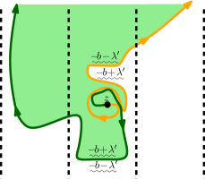
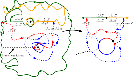
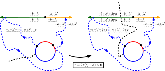
Lemma 5.6.
Let be the connected component of which contains . Then
-
(i)
can be expressed as a (possibly degenerate) disjoint union of one segment of and one segment of ; see Figure 5.7.
-
(ii)
Almost surely, as (where is the starting point of ).
Proof.
The first assertion follows from Lemma 5.4 as well as the argument described in Figure 5.5 and Figure 5.6. To see the second assertion of the lemma, we first condition on and then consider two possibilities. Either:
-
1.
The range of contains self-intersection points with arbitrarily large modulus.
-
2.
The range of does not contain self-intersection points with arbitrarily large modulus.
In the former case, the transience of implies that for every there exists such that if then the distance of the connected component of containing to is at least . By increasing if necessary the same is also true for all of the pockets of which come after in the order given by the order in which traces part of the boundary of such a pocket. Say that two pockets of are adjacent if the intersection of their boundaries contains the image under of a non-trivial interval. Fix and let denote the union of the pockets of that can be reached from by jumping to adjacent pockets at most times. By the same argument, there exists such that if then . The same likewise holds for the pockets which come after those which make up . Combining this with the first assertion of the lemma implies the second assertion in this case.
The argument for the latter case is similar to the proof of [MS16d, Proposition 7.33]. We let be the unbounded connected component of and be a conformal map which fixes and sends the final self-intersection point of to . We let where is the GFF on used to define and as in Lemma 5.4. We note that the boundary conditions of are piecewise constant, changing only once at . Let . Then it suffices to show that the diameter of the connected component of which contains becomes unbounded as tends to in . To see this, we let be flow lines of starting from with equally spaced angles such that almost surely intersects both and for each . Here, we take and . By Lemma 5.4 there exists such that can cross each of the at most times. Let .
Say that two connected components of are adjacent if the intersection of the boundaries of and contains the image of a non-trivial interval of for some . We also say that comes after if there exists such that both and lie between and and the boundary of is traced by after it traces the boundary of . Let be the connected component of which contains and let be the closure of the union of the connected components which can be reached in at most steps starting from or comes after such a component. By Lemma 5.4, , so it suffices to show that
| (5.3) |
Since each is almost surely transient as a chordal process in from to with (where the weights depend on ) and almost surely has intersections with both of its neighbors with arbitrarily large modulus, it follows that
| (5.4) |
The same is likewise true for all of the pockets which can be reached from in at most steps as well as for the pockets which come after these. This proves (5.3), hence the second assertion of the lemma. ∎
By Lemma 5.5, we know how to resample given . Similarly, we know how to resample given . Indeed, in each case is given by a flow line of a GFF on for . We will now argue that given as well as initial segments of and , the conditional law of until crossing is uniquely determined by the resampling property and can be described in terms of GFF flow lines (see Figure 5.7).
| Range of values for | Behavior of blue path in Figure 5.7 |
|---|---|
| if it hits as shown | |
| Cannot hit (without going around the disk). | |
| Can hit green only, reflects left afterward. | |
| Can hit green only, merges with green. | |
| Can hit either color, crosses afterward. | |
| Can hit orange only, merges with orange. | |
| Can hit orange only, reflects right. | |
| Cannot hit (without going around the disk). |
Lemma 5.7.
Suppose that for is an almost surely positive and finite stopping time for . Let be the event that is contained in the connected component of which contains . On , let be the connected component of whose boundary intersects . Then the conditional law of stopped upon exiting given , , (where is the GFF on used to generated ) is that of a pair of flow lines of a GFF on whose boundary behavior agrees with that of and with angles as implied by the resampling property for and .
Proof.
The proof is similar to that of [MS16e, Theorem 4.1]. Suppose that is a GFF on whose boundary conditions are as described in the statement of the lemma (given ) and let be the flow lines of starting from with the same angles as (are implied for) . Then for and , we know that the conditional law of given and for is the same as that of given and . Moreover, is homotopic to since the boundary conditions for force the net winding of around the inner boundary of to be the same as as that of (where both pairs are stopped upon exiting ).
The resampling property for implies that it is a stationary distribution for the following Markov chain. Its state space consists of pairs of continuous, non-crossing paths in where connects to for . The transition kernel is given by first picking uniformly and then resampling by:
-
1.
Picking a GFF on for distinct from with boundary data agrees with and has -flow line boundary conditions with the same angle as (is implied for) along .
-
2.
Taking the flow line starting from with the same angle as (is implied for) stopped upon first exiting .
As explained in [MS16e, Section 4], any such ergodic measure which arises in the ergodic decomposition of either the law of or must be supported on path pairs which are:
-
1.
homotopic to in
-
2.
there exists (possibly random) such that the number of times a path hits any point in is almost surely at most .
Indeed, as we mentioned earlier, almost surely satisfies the first property due to the boundary data of . The second property is satisfied for by transience and continuity. The discussion in Section 3.6 implies that also satisfies the second property. To complete the proof it suffices to show that there is only one such ergodic measure. Suppose that are such ergodic measures and that (resp. ) is distributed according to (resp. ). Then it suffices to show that we can construct a coupling such that since this implies that and are not be mutually singular, hence equal by ergodicity.
As explained in Figure 5.7 and Figure 5.8 as well as in Table 1, it might be that the strands of (resp. ) exit the same point or distinct points, depending on the boundary data along . Moreover, in the former case the strands exit at the point on which is last drawn by the strands of (the “closing point” of the pocket; in the right side of Figure 5.7 this point corresponds to in ). Thus by possibly drawing a segment of a counterflow line starting from , we may assume without loss of generality that we are in the latter setting. Indeed, this is similar to the trick used in [MS16e, Section 4].
Recall that we can describe the conditional law of given (and the boundary heights) in in terms of a flow line of a GFF on and the same is likewise true with in place of . Thus by Lemma 5.2, Lemma 3.8, and Lemma 3.9, it follows that we can couple and together such that there exists a positive probability event on which each is a -tangle in and is much closer to for than is to , . Thus by working on and first resampling given , absolute continuity for the GFF implies that we can recouple the paths together so that with positive probability (see [MS16e, Lemma 4.2]). On this event, the resampling property for (resp. ) given (resp. ) implies that we can couple the laws together so that with positive conditional probability. This proves the existence of the desired coupling, which completes the proof. ∎
We can now complete the proof of Theorem 5.1.
Proof of Theorem 5.1.
Fix and let for be the first time that hits . Fix very large and with sufficiently large so that (by Lemma 5.6) it is unlikely that the connected component of containing intersects . Let be the GFF on used to generate . Let and be as in Lemma 5.7 where we take the stopping times for as above. By Lemma 5.7, we know that the conditional law of given for , , , and is described in terms of a pair of flow lines of a GFF on . Let be a conformal transformation which takes to an annulus and let . Then we can write where is a zero-boundary GFF and is a harmonic function. The boundary conditions for are given by (resp. ) on the inner (resp. outer) boundary of the annulus, up to a bounded additive error which does not depend on or . (The error comes from times the winding of the two annulus boundaries, additive terms of depending on whether the boundary segment is the image of the left or the right side of one of the or , and finally from the angles of the different segments.) The value of is determined by the resampling property for . In particular, away from the annulus boundary it is clear that is well-approximated by an affine transformation of the function. Indeed, this follows because is well-approximated by the function which is harmonic in the annulus with boundary values on the annulus boundaries given by the corresponding average of and the functions which are harmonic in an annulus and take on a constant value on the inner and outer annulus boundaries (i.e., radially symmetric) are exactly the affine transformations of the function. Thus by sending and , we see that converges to a multiple of the function (modulo additive constant). The measure in the statement of the theorem is exactly given by the law of the multiple of the function. ∎
5.3 Proof of Theorem 1.20
Fix , , and let . By adjusting the value of , we note that can take on any value in . Let be a whole-plane GFF and , viewed as a distribution defined up to a global multiple of . By Theorem 1.4, the flow line of starting from with zero angle is a whole-plane process. Let and let be the flow line of starting from with angle . Note that this choice of lies exactly in the middle of the available range. For , let denote the time-reversal of . By Theorem 5.1 and the main result of [MS16e], we know that the conditional law of given is the same as that of given and the same also holds when the roles of and are swapped. Consequently, it follows that the joint law of the image of the pair of paths under is described (up to reparameterization) by
where is a probability measure on and is as defined in Theorem 5.1. In order to complete the proof of Theorem 1.20 for , we need to show that . This in turn is a consequence of the following proposition.
Proposition 5.8.
Suppose that , , , and that is a whole-plane process. For each , let (resp. ) be the first (resp. last) time that hits . For each with , let be the number of times that winds around (rounded down to the nearest integer). For each we almost surely have that
In particular, the value of is almost surely determined by and is invariant under time-reversal/inversion.
The statement of Proposition 5.8 is natural in view of Theorem 1.4 and Proposition 3.18. We emphasize that the winding is counted positively (resp. negatively) when travels around the origin in the counterclockwise (resp. clockwise) direction. The main step in the proof of Proposition 5.8 is the following lemma, which states that the harmonic extension of the winding of a curve upon getting close to (and evaluated at) a given point is well approximated by the winding number at this point.
Lemma 5.9.
There exists a constant such that the following is true. Suppose that is a continuous curve in connecting to with continuous radial Loewner driving function . Fix , let , and let be the number of times that winds around (rounded down to the nearest integer). We have that
The quantity in the statement of Lemma 5.9 is called the twisting of upon hitting . An estimate very similar to Lemma 5.9 was proved in an unpublished work of Schramm and Wilson [SW].
Proof of Lemma 5.9.
Let be the concatenation of with the curve that travels along the straight line segment starting at towards until hitting and then traces (all of) in the counterclockwise direction. Let be the time that finishes tracing and let be the number of times that winds around . Then
| (5.5) |
Let be the radial Loewner evolution associated with , its radial Loewner driving function, and . Note that
That is, is equal to the value of the harmonic function evaluated at . We claim that there exists a constant such that
| (5.6) |
If is a piecewise smooth curve then the boundary values of along differ from by at most a constant . Thus the claim follows in this case since is harmonic in . The claim for general continuous curves follows by approximation and [Law05, Proposition 4.43]. Observe that
| (5.7) |
Proof of Proposition 5.8.
The second assertion of the proposition is an immediate consequence of the first, so we will focus our attention on the latter.
We begin by letting be the number of times that winds around (rounded down to the nearest integer). By the scale invariance of whole-plane , the law of the number of times that winds around does not depend on . Moreover, by the transience of whole-plane (Theorem 1.12) we have that this quantity is finite almost surely. Consequently, it is not difficult to see that
almost surely. In particular, it suffices to prove the result with in place of .
Suppose that where is a GFF on such that has the same boundary values as illustrated in the left side of Figure 3.1 where we take . Let be the flow line of starting from and . As explained in the proof of Proposition 3.18, the random curve converges to a whole-plane process as . Consequently, it suffices to prove the result with in place of and the hitting times in place of . Let denote the radial Loewner driving function associated with and, for each , let . By Lemma 5.9, it suffices to show that
(the reason for the sign difference from the statement of Proposition 5.8 is that the inversion reverses the direction in which the path winds). For each let denote the average of on . The conditional law of given is that of a Gaussian random variable with mean and bounded variance (see [DS11, Proposition 3.2]). Consequently, it suffices to show that
This follows because for each , is equal in law to a Gaussian random variable with mean and variance (see [DS11, Proposition 3.2]). ∎
We will now complete the proof of Theorem 1.20 for . Suppose that is a whole-plane process for and . Theorem 1.15 implies that the outer boundary of is described by a pair of whole-plane GFF flow lines, say and with angle gap . Consequently, it follows from Theorem 1.20 applied for that we can construct a coupling of with a whole-plane process from to such that the left and right boundaries of are almost surely equal to . Theorem 1.15 implies that the conditional law of given and in each of the connected components of which lie between and is independently that of a chordal process going from the first point on the component boundary drawn by and to the last. The same is also true for but with the roles of the first and last points swapped. Consequently, it follows from the main result of [MS16f] that we can couple and together so that is almost surely the time-reversal of . This completes the proof for for . The result for follows by taking a limit , which completes the proof of Theorem 1.20. ∎
Remark 5.10.
The same proof applies if we add a multiple of . It implies that the whole-plane SLE path drawn from to with non-zero drift (and possibly non-zero ) has a law that is preserved when we reverse time (up to monotone parameterization) and map the plane to itself via .
References
- [Ald91a] D. Aldous. The continuum random tree. I. Ann. Probab., 19(1):1–28, 1991. MR1085326 (91i:60024)
- [Ald91b] D. Aldous. The continuum random tree. II. An overview. In Stochastic analysis (Durham, 1990), volume 167 of London Math. Soc. Lecture Note Ser., pages 23–70. Cambridge Univ. Press, Cambridge, 1991. MR1166406 (93f:60010)
- [Ald93] D. Aldous. The continuum random tree. III. Ann. Probab., 21(1):248–289, 1993. MR1207226 (94c:60015)
- [Bef08] V. Beffara. The dimension of the SLE curves. Ann. Probab., 36(4):1421–1452, 2008. math/0211322. MR2435854 (2009e:60026)
- [DMS14] B. Duplantier, J. Miller, and S. Sheffield. Liouville quantum gravity as a mating of trees. ArXiv e-prints, September 2014, 1409.7055.
- [DS11] B. Duplantier and S. Sheffield. Liouville quantum gravity and KPZ. Invent. Math., 185(2):333–393, 2011. 0808.1560. MR2819163 (2012f:81251)
- [Dub09a] J. Dubédat. Duality of Schramm-Loewner evolutions. Ann. Sci. Éc. Norm. Supér. (4), 42(5):697–724, 2009. 0711.1884. MR2571956 (2011g:60151)
- [Dub09b] J. Dubédat. SLE and the free field: partition functions and couplings. J. Amer. Math. Soc., 22(4):995–1054, 2009. 0712.3018. MR2525778 (2011d:60242)
- [HBB10] C. Hagendorf, D. Bernard, and M. Bauer. The Gaussian free field and on doubly connected domains. J. Stat. Phys., 140(1):1–26, 2010. 1001.4501. MR2651436 (2011d:60243)
- [IK13] K. Izyurov and K. Kytölä. Hadamard’s formula and couplings of SLEs with free field. Probab. Theory Related Fields, 155(1-2):35–69, 2013. 1006.1853. MR3010393
- [Ken01] R. Kenyon. Dominos and the Gaussian free field. Ann. Probab., 29(3):1128–1137, 2001. math-ph/0002027. MR1872739 (2002k:82039)
- [KS91] I. Karatzas and S. E. Shreve. Brownian motion and stochastic calculus, volume 113 of Graduate Texts in Mathematics. Springer-Verlag, New York, second edition, 1991. MR1121940 (92h:60127)
- [Law05] G. F. Lawler. Conformally invariant processes in the plane, volume 114 of Mathematical Surveys and Monographs. American Mathematical Society, Providence, RI, 2005. MR2129588 (2006i:60003)
- [Law11] G. F. Lawler. Continuity of radial and two-sided radial at the terminal point. ArXiv e-prints, April 2011, 1104.1620.
- [LSW04] G. F. Lawler, O. Schramm, and W. Werner. Conformal invariance of planar loop-erased random walks and uniform spanning trees. Ann. Probab., 32(1B):939–995, 2004. math/0112234. MR2044671 (2005f:82043)
- [MS10] N. Makarov and S. Smirnov. Off-critical lattice models and massive SLEs. In XVIth International Congress on Mathematical Physics, pages 362–371. World Sci. Publ., Hackensack, NJ, 2010. 0909.5377. MR2730811
- [MS15a] J. Miller and S. Sheffield. An axiomatic characterization of the Brownian map. ArXiv e-prints, June 2015, 1506.03806.
- [MS15b] J. Miller and S. Sheffield. Liouville quantum gravity and the Brownian map I: The QLE(8/3,0) metric. ArXiv e-prints, July 2015, 1507.00719.
- [MS15c] J. Miller and S. Sheffield. Liouville quantum gravity spheres as matings of finite-diameter trees. ArXiv e-prints, June 2015, 1506.03804.
- [MS16a] J. Miller and S. Sheffield. Gaussian free field light cones and SLE. ArXiv e-prints, June 2016, 1606.02260.
- [MS16b] J. Miller and S. Sheffield. Liouville quantum gravity and the Brownian map II: geodesics and continuity of the embedding. ArXiv e-prints, May 2016, 1605.03563.
- [MS16c] J. Miller and S. Sheffield. Liouville quantum gravity and the Brownian map III: the conformal structure is determined. ArXiv e-prints, August 2016, 1608.05391.
- [MS16d] J. Miller and S. Sheffield. Imaginary geometry I: interacting SLEs. Probab. Theory Related Fields, 164(3-4):553–705, 2016. 1201.1496. MR3477777
- [MS16e] J. Miller and S. Sheffield. Imaginary geometry II: reversibility of for . Ann. Probab., 44(3):1647–1722, 2016. 1201.1497. MR3502592
- [MS16f] J. Miller and S. Sheffield. Imaginary geometry III: reversibility of for . Ann. of Math. (2), 184(2):455–486, 2016. 1201.1498. MR3548530
- [MS16g] J. Miller and S. Sheffield. Quantum Loewner evolution. Duke Math. J., 165(17):3241–3378, 2016. 1312.5745. MR3572845
- [MSW16] J. Miller, S. Sheffield, and W. Werner. CLE percolations. ArXiv e-prints, February 2016, 1602.03884.
- [MW17] J. Miller and H. Wu. Intersections of SLE Paths: the double and cut point dimension of SLE. Probab. Theory Related Fields, 167(1-2):45–105, 2017. 1303.4725. MR3602842
- [RS] S. Rohde and O. Schramm. Unpublished.
- [RS05] S. Rohde and O. Schramm. Basic properties of SLE. Ann. of Math. (2), 161(2):883–924, 2005. math/0106036. MR2153402 (2006f:60093)
- [RY99] D. Revuz and M. Yor. Continuous martingales and Brownian motion, volume 293 of Grundlehren der Mathematischen Wissenschaften [Fundamental Principles of Mathematical Sciences]. Springer-Verlag, Berlin, third edition, 1999. MR1725357 (2000h:60050)
- [Sch00] O. Schramm. Scaling limits of loop-erased random walks and uniform spanning trees. Israel J. Math., 118:221–288, 2000. math/9904022. MR1776084 (2001m:60227)
- [She] S. Sheffield. Local sets of the gaussian free field: slides and audio. www.fields.utoronto.ca/0506/percolationsle/sheffield1, www.fields.utoronto.ca/audio/0506/percolationsle/sheffield2, www.fields.utoronto.ca/audio/0506/percolationsle/sheffield3.
- [She07] S. Sheffield. Gaussian free fields for mathematicians. Probab. Theory Related Fields, 139(3-4):521–541, 2007. math/0312099. MR2322706 (2008d:60120)
- [She09] S. Sheffield. Exploration trees and conformal loop ensembles. Duke Math. J., 147(1):79–129, 2009. math/0609167. MR2494457 (2010g:60184)
- [She16a] S. Sheffield. Conformal weldings of random surfaces: SLE and the quantum gravity zipper. Ann. Probab., 44(5):3474–3545, 2016. 1012.4797. MR3551203
- [She16b] S. Sheffield. Quantum gravity and inventory accumulation. Ann. Probab., 44(6):3804–3848, 2016. 1108.2241. MR3572324
- [SS13] O. Schramm and S. Sheffield. A contour line of the continuum Gaussian free field. Probab. Theory Related Fields, 157(1-2):47–80, 2013. 1008.2447. MR3101840
- [SW] O. Schramm and D. B. Wilson. Private communication.
- [SW05] O. Schramm and D. B. Wilson. SLE coordinate changes. New York J. Math., 11:659–669 (electronic), 2005. MR2188260 (2007e:82019)
- [SW12] S. Sheffield and W. Werner. Conformal loop ensembles: the Markovian characterization and the loop-soup construction. Ann. of Math. (2), 176(3):1827–1917, 2012. 1006.2374. MR2979861
- [Wer04] W. Werner. Random planar curves and Schramm-Loewner evolutions. In Lectures on probability theory and statistics, volume 1840 of Lecture Notes in Math., pages 107–195. Springer, Berlin, 2004. math/0303354. MR2079672 (2005m:60020)
- [Wil96] D. B. Wilson. Generating random spanning trees more quickly than the cover time. In Proceedings of the Twenty-eighth Annual ACM Symposium on the Theory of Computing (Philadelphia, PA, 1996), pages 296–303. ACM, New York, 1996. MR1427525
- [Zha08a] D. Zhan. Duality of chordal SLE. Invent. Math., 174(2):309–353, 2008. 0712.0332. MR2439609 (2010f:60239)
- [Zha08b] D. Zhan. Reversibility of chordal SLE. Ann. Probab., 36(4):1472–1494, 2008. 0808.3649. MR2435856 (2010a:60284)
- [Zha10a] D. Zhan. Duality of chordal SLE, II. Ann. Inst. Henri Poincaré Probab. Stat., 46(3):740–759, 2010. 0803.2223. MR2682265 (2011i:60155)
- [Zha10b] D. Zhan. Reversibility of some chordal traces. J. Stat. Phys., 139(6):1013–1032, 2010. 0807.3265. MR2646499 (2011h:60174)
- [Zha15] D. Zhan. Reversibility of whole-plane SLE. Probab. Theory Related Fields, 161(3-4):561–618, 2015. 1004.1865. MR3334276
Microsoft Research
One Microsoft Way
Redmond, WA, USA
Department of Mathematics
Massachusetts Institute of Technology
Cambridge, MA, USA