The 2013 Release of Cloudy

Abstract

This is a summary of the 2013 release of the plasma simulation code Cloudy. Cloudy models the ionization, chemical, and thermal state of material that may be exposed to an external radiation field or other source of heating, and predicts observables such as emission and absorption spectra. It works in terms of elementary processes, so is not limited to any particular temperature or density regime. This paper summarizes advances made since the last major review in 1998. Much of the recent development has emphasized dusty molecular environments, improvements to the ionization / chemistry solvers, and how atomic and molecular data are used. We present two types of simulations to demonstrate the capability of the code. We consider a molecular cloud irradiated by an X-ray source such as an Active Nucleus and show how treating EUV recombination lines and the full SED affects the observed spectrum. A second example illustrates the very wide range of particle and radiation density that can be considered.

Este es un resumen de la versión 2013 del código Cloudy para simulación de plasmas. Cloudy modela el estado térmico, químico y de ionización de la materia que puede ser expuesta a un campo de radiación externa u otras fuentes de calentamiento, y predice cantidades observables tales como los espectros de emisión y absorción. El código trabaja en términos de procesos elementales y, por lo tanto, no es limitado a un rango particular de densidad o temperatura. Este artículo resume los avances logrados desde la última reseña de mayo de 1998. Mucho del desarrollo reciente se ha enfatizado en los ambientes moleculares polvosos, en mejoras a los resolvedores de ionización/química, y en la forma de uso de los datos atómicos y moleculares. Presentamos dos tipos de simulaciones para demostrar las capacidades del código. Consideramos una nube molecular irradiada por una fuente de rayos X, por ejemplo, un Núcleo Activo, e ilustramos el efecto sobre el espectro observado de líneas de recombinación EUV y de la distribución espectral completa de la radiación. Un segundo ejemplo destaca el rango tan amplio de densidad de partículas y de radiación que se puede considerar.

atomic processes galaxies: active methods: numerical molecular processes radiation mechanisms 1 2013

1.1

0.1 Introduction

Most quantitative information we have about the cosmos comes from spectroscopy. In many astronomical environments the density is too low for equilibrium thermodynamics to apply, so the ionization, molecular state, level populations, kinetic temperature, and the resulting spectrum are the result of a host of microphysical processes. As a result the spectrum reveals much about the properties of an object, but it also means that modeling this detail is complex. Analytical results are only possible in certain limits, so numerical simulations must be used. Texts that review this field include Spitzer (1978), Dopita & Sutherland (2003), Tielens (2005), Osterbrock & Ferland (2006) (hereafter AGN3), and Draine (2011).

Cloudy is an open source plasma simulation code that is designed to simulate conditions in a non-equilibrium gas, and predict its spectrum. The code incorporates physical processes from first principles, as much as possible. The goal is to simulate the ionization, level populations, molecular state, and thermal state, over all extremes of density and temperature. Our approach, working from fundamental processes, means that Cloudy can be applied to such diverse regions as the corona of a star, the intergalactic medium, or the accretion disk near the supermassive black hole in a luminous quasar. As a result, the code is widely used, with nearly 200 papers citing its documentation each year. The diversity of problems it can address is a testimonial to the importance of treating the atomic physics at an elementary level.

Processor power has always limited our ability to simulate detailed microphysics. Improved computers and advances in atomic and molecular physics allow a better simulation. Improved numerical methods or coding techniques make the solutions more robust. These advancements to the fidelity of the simulation improve our insight into the inner workings of astronomical objects. Because of these changes, Cloudy, like most software, goes through a development / release cycle. Our goal is to make major updates every two or three years.

This paper is a progress report on the improvements to Cloudy since the last major review, Ferland et al. (1998), referred to as F98 in the following. Although the code’s download includes extensive documentation that is continuously updated, there has not been a recent major review. We rectify that need here.

Cloudy’s development leading up to the 1998 review had emphasized the UV, optical, and IR spectra of ionized gas. The simulations have been extended to fully molecular regions with predictions of the associated IR and radio emission since then. The code can handle a broad range of physical state, from predominantly molecular to fully ionized, a broad range of densities from the low density limit to roughly $10^{15}{\rm\thinspace cm^{-3}}$, and temperatures ranging from the CMB to $10^{10}{\rm\thinspace K}$.

In the present paper, we summarize the major advances in the code since F98. Most of this work has been documented in past papers, which we cite. In the interests of brevity we only give references to the relevant papers with a brief summary of the advances they document. We discuss some technical details about the code, its operation, and installation. We present several calculations that show the range of applicability of Cloudy. These include the properties of the ionized, atomic, and molecular gas produced by the radiation field of an Active Galactic Nucleus (AGN) and a demonstration of the range of particle and radiation density that can be considered. We conclude with an outline of future development directions.

0.2 The physics of ions, molecules, and grains

Cloudy was originally designed to simulate the dense gas found near the black hole and accretion disk in AGN. The so-called “Broad Line Region” (BLR) mainly emits in the UV and optical, and these spectral regimes were the original focus. Some investigations are Rees et al. (1989), Ferland et al. (1992), and Baldwin et al. (1995). Lower density gas, at larger distances from the center, produces the “Narrow Line Region” (NLR) spectrum, which includes a range of forbidden and permitted lines in the UV, optical, and IR. The study by Ferland & Netzer (1983) is an example. Such investigations drove the development of Cloudy, as summarized in the 1998 review, although Photo-dissociation Region (“PDRs”) and X-ray Dissociation Regions (“XDRs”) were also simulated (Ferland et al., 1994, 2002).

The following sections describe our improvements in the treatment of ions, molecules, and grains since F98, by citing those papers which introduced the advances. This is not meant to be a comprehensive review of the literature, rather, only a description of advances to Cloudy since the last review.

0.2.1 Structure of the H-like and He-like iso-electronic sequences

Hydrogen and helium are the most common elements in the universe and, as a result, need to be treated with the greatest precision. Their structure is different from most heavy elements, with a first excited level at (1-1/$n^{2}$) = 0.75 of the ionization energy and more highly excited levels close to the ionization limit. By contrast, the heavy elements can have many low-lying levels. This means that, for most temperatures, lines from H and He – like species will have a strong recombination component, while lines of many-electron systems will be predominantly collisionally excited. The structure of the H and He – like iso sequences also means that a significant number of excited states are needed for the model atoms to correctly go to LTE in the high particle or photon limits.

Steve Cota developed the original model of H 1, He 1, and He 2 emission in Cloudy as part of his PhD thesis (Cota, 1987). He also developed an approximate treatment of three-body recombination for the heavy elements, described in the next section. This was extended by Jason Ferguson in his PhD thesis (Ferguson, 1997; Ferguson & Ferland, 1997) to include more levels, as processor power increased. These models, which involved 15 levels with a number of higher pseudo states, were significant time sinks on the computers at that time.

Today’s unified model of the H and He iso-electronic sequences was developed as part of Ryan Porter’s thesis. Because the high charge states occur in hot gas and the line energies scale as $Z^{2}$, these iso-sequences sort themselves into two spectral regions. H 1, He 1, and He 2  produce strong lines in the optical while C 5, C 6, O 7, O 8, Fe 25, Fe 26, etc produce lines in the X-ray. Despite these differences, the physics has many similarities. These sequences are treated with a common code base, which results in greater simplicity and reliability.

Porter et al. (2005) and Bauman et al. (2005) describe the model of He 1 emission. Porter & Ferland (2007) describe ions of the He sequence, which mainly emits in the X-Ray. Luridiana et al. (2009) summarize expansions to the H-like sequence while Porter et al. (2007), Porter et al. (2009), and Porter et al. (2012) discuss uncertainties and more recent improvements in the atomic data for He 1.

A schematic representation of one of the elements of the H-sequence is shown in Figure 1. The He-sequence has similar structure except that it is resolved into singlets and triplets with twice as many levels. Principal quantum number increases upward with the continuum at the top and $nl$ terms are indicated from left to right. Lower $n$ configurations are resolved into $nl$ terms, the “resolved” levels. Above a certain quantum number $l$-changing collisions become fast enough to guarantee that $l$ terms are populated according to their statistical weight within the $n$ configuration (Pengelly & Seaton, 1964). Such higher levels are treated as “collapsed levels” which are $nl$ mixed.

Figure 1: The iso-sequence atomic level structure consists of low-lying $nl$ resolved ($nls$ for He-like) terms with $l-$mixed ($ls$ for He-like) collapsed configurations. The number of resolved and collapsed levels can be specified when the simulation parameters are established.

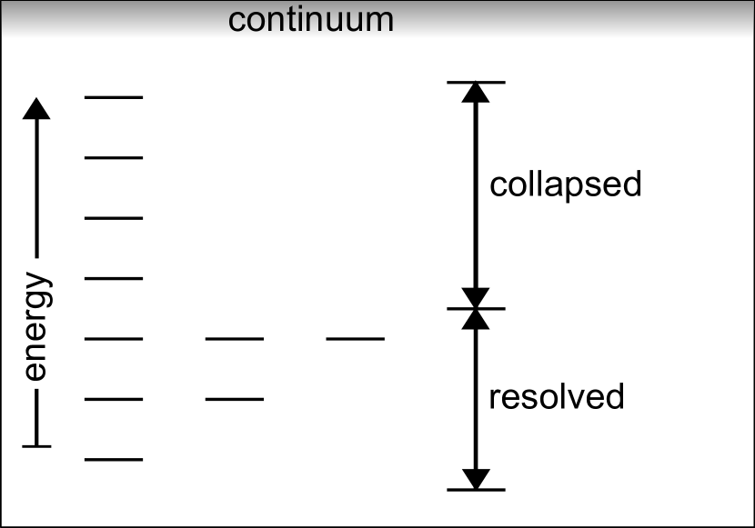
This treatment includes ions of all elements up to Zinc. The models include photoionization / recombination, collisional ionization / 3-body recombination, to all levels, and collisional and radiative processes between levels, so behave correctly in the low density limit and go to LTE at high densities or exposed to a true blackbody radiation field (Ferland & Rees, 1988). Line trapping, collisions, continuum lowering, and absorption of photons by continuous opacities, are all included as general processes (Rees et al., 1989).

The user can adjust the number of resolved and collapsed levels modeled when the simulation is specified. The spectrum is predicted with great precision, an accuracy of better than 1%, when a larger number of levels are used (Porter et al., 2012). This comes at the cost of increased execution times. Smaller models are often used for simulations of clouds with significant column densities due to the compute time required. The default treatment includes the greatest number of levels for H, and increasingly smaller numbers of levels for He, common second row elements like C and O, Fe, and the remaining low abundance elements.

0.2.2 Structure of other ions

Cloudy includes all ions of the lightest thirty elements. Lykins et al. (2013) summarize recent developments in the treatment of the ions that are not part of the H and He iso-sequences.

An equivalent two-level system is assumed in modeling the ionization balance of ions of the Li-like and multi-electron iso sequences. Photoionization and collisional ionization from the ground configuration is balanced by recombinations to all levels. This assumes that nearly all populations are in ground, an approximation which is valid for moderate densities and the low temperatures usually found in photoionization equilibrium. Photoionization cross sections are from the Verner database (Verner et al., 1996) while radiative and dielectronic recombination rates are largely from the Badnell web site as described in Badnell et al. (2003) and Badnell (2006), supplemented by data calculated as described by Verner & Ferland (1996). Charge exchange ionization and recombination rates are taken from an updated version of the Kingdon & Ferland (1996) database.

The treatment of inner-shell processes, including line emission following removal of an inner-shell electron, largely follows F98. As described below, the treatment of multiple electron ejection, which had followed Weisheit & Dalgarno (1972), is now generalized to non-adjacent stages of ionization (Henney et al., 2005). Ionization and recombination coupling non-adjacent ion states can also be important in grain surface recombination.

This treatment is approximate at high densities and for temperatures which are a significant fraction of the ionization potential of a species. The use of summed recombination rate coefficients in effect assumes that all recombinations eventually populate the ground level. Ionization processes out of excited levels are neglected. Both are no longer true if the density is large enough for excited levels to play an important role. Expanding the treatment of these species to the approach now used for the H and He iso sequences is a high priority for future development.

Bound levels of each ion are treated with a variety of models. We are enhancing the code to use external databases as much as possible. We have the ability to read the Chianti atomic database (Dere et al., 1997; Landi et al., 2012) and this release of Cloudy includes Version 7.0. Chianti is used for most ions of Fe while for other species we mainly use our internally developed atomic database. Lykins et al. (2013) shows that our original database, which is embedded in the C++ source, is in good agreement with Chianti.

Additionally we are starting to develop our own database, “Stout”. We will add new models of ions or molecules to this second database, and make it publicly available along with Cloudy.

0.2.3 Molecular chemistry

Cloudy initially included the chemistry network described by Black (1978) which was expanded to treat PDRs and XDRs as described by Ferland et al. (1994). Nick Abel carried out a massive upgrade to the heavy-element chemistry network as part of his PhD thesis, described in Abel et al. (2004). Later refinements are discussed in Abel et al. (2005), Shaw et al. (2005), and Shaw et al. (2006). Appendix A of Abel et al. (2005) gives details of the numerical methods along with differences between UMIST and Cloudy reaction rates. Cloudy had predicted column densities for about 20 heavy element molecules, consisting of C and O atoms. It could not calculate physical conditions deep in a PDR or a molecular cloud, where most gas phase C, N, and O is in the form of molecules, due to numerical instabilities in the chemistry solver then used. The upgraded chemistry solver has no restrictions, as described in sections below. Cloudy now calculates the chemical abundance of 83 molecules using a network including $\sim 10^{3}$ chemical reactions involving molecules containing H, He, C, N, O, Si, S, and Cl atoms. The network adjusts automatically when elements or species are disabled.

Most reaction rates come from the UMIST 2000 database (Le Teuff et al., 2000) as updated for the Leiden workshop and described by Röllig et al. (2007). We also predict the freeze-out of H₂O, CO, and OH on grains, using the data given in Hasegawa & Herbst (1993). Both time-steady and time-dependent chemical evolution calculations are possible.

The effects of cosmic rays and suprathermal secondary electrons can be very important in molecular regions (Spitzer & Tomasko, 1968) and are treated as described by Ferland & Mushotzky (1984) and Ferland et al. (2009). Non-thermal particles can both excite and dissociate the gas. Ferland et al. (1994) and Ferland et al. (2002) describe the treatment of chemistry in an X-ray dominated filaments in cool-core galaxy clusters. Shaw et al. (2008) describe an application to the local ISM.

The treatment of H₂ is fully self consistent with its surroundings (Shaw et al., 2005). Formation on grain surfaces is treated using the derived grain properties and the Cazaux & Tielens (2004) catalysis rates. Destruction by photoexcitation in electronic states is treated by computing the radiation field at each point. This includes line self shielding, the attenuation by continuous opacity sources such as grains, photoelectric opacity of the heavy elements, and Rayleigh scattering, and emission by the cloud itself. H i L$\alpha$, the He 1 resonance lines, and electronic lines of H₂ are especially important sources of higher-energy photons.

0.2.4 Molecular excitations and spectra

We next describe our treatment of molecular emission processes. Gargi Shaw developed our model of the H₂ molecule, the most common molecule in the Universe, as part of her PhD thesis (Shaw et al., 2005). All levels within the ground electronic state are included (Dabrowski, 1984), along with all electronic excited states on the Meudon web site and Abgrall et al. (1994). Collision rates are from Wrathmall et al. (2007). Lee et al. (2005, 2006, 2008), Shaw et al. (2009), and Gay et al. (2012) summarize more recent updates.

Grain formation pumping of H₂ can be treated using several theories. Shaw et al. (2005) provides more details. We use the Takahashi (2001) results by default.

Line emission for molecules heavier than H₂ is predicted using the level energy, collision, and radiative data in the LAMDA database (Schöier et al., 2005). The molecular excitation are solved simultaneously and self-consistently with the global environment. This includes grain properties, including emission, so molecular pumping in the infrared continuum is automatically included (if the pumping lines are present in the molecular data), along with attenuation by grains and other continuous opacity sources. Line optical depths are computed for each point in the cloud, and the full radiative transfer performed as described below.

0.2.5 Grains

Grains have been included in Cloudy since the very beginning (Martin & Ferland, 1980), and the basic physical processes are summarized in Appendix C of Baldwin et al. (1991). van Hoof et al. (2004) describe the main improvements made since Baldwin et al. (1991).

The grain model in Cloudy includes all relevant processes: absorption and scattering of light including stochastic heating effects, the photoelectric effect including Auger emissions in X-ray environments, collisional charging (electrons as well as atomic ions), thermionic emissions, collisional energy exchange between the grains and the gas, and a calculation of the grain drift velocity. We also consider molecular freeze-out on grain surfaces and grain surface reactions. These are discussed in Section 0.2.3.

The local radiation field, including the attenuated incident Spectral Eenergy Distribution (SED) and the spectrum emitted by the cloud (generally L$\alpha$ is the most important) are all treated self-consistently, with gas and grains providing the opacity affecting the light, and the light affecting the grain properties following absorption. The code fully treats stochastic heating of grains using a robust and efficient algorithm (which is a comprehensively upgraded version of a code originally written by K. Volk), implementing an improved version of the procedure described in Guhathakurta & Draine (1989). This includes an approximate treatment for stochastic heating by particle collisions. Combined with resolved size distributions, this will lead to a much more realistic modeling of the grain emission under all circumstances. The stochastic heating code needs a grain enthalpy function. Supported functions are taken from Guhathakurta & Draine (1989), Dwek et al. (1997), and Draine & Li (2001).

The grain physics includes the advances discussed by Weingartner & Draine (2001) and Weingartner et al. (2006). The latter provides a realistic model for grains in X-ray environments, including Auger emissions by the grains. The grain model has a detailed treatment of the photoelectric effect and collisional processes, and includes thermionic emissions. The charge for each grain constituent is determined self consistently with the local radiation field and gas properties, using the hybrid grain charge model described by van Hoof et al. (2001) and van Hoof et al. (2004). The grain charge is included in the overall charge balance of the system, which has a significant effect on the modeling results for molecular regions (Abel et al., 2008). Charge exchange on grain surfaces is treated following Draine & Sutin (1987) assuming that electrons will be exchanged between the grain and the colliding particle until a minimum energy state is reached. The grain drift velocity w.r.t. the gas is calculated using the theory from Draine & Salpeter (1979).

Extensive comparisons in collaboration with Joe Weingartner done in 2001 show that the photoelectric heating rates and collisional cooling rates predicted by Cloudy agree very well with the results from the Weingartner & Draine (2001) model for a wide range of grain sizes (between 5 Å and 0.1 $\mu$m), and using various choices for the incident radiation field. A detailed discussion of this comparison can be found in van Hoof et al. (2001).

We include an embedded model for Mie scattering (Mie, 1908), which uses refractive index data for each material type. It is based on the code described in Hansen & Travis (1974) and was later modified by P.G. Martin. New grain materials can be included by specifying the relevant refractive index data or by supplying opacity tables. The user specifies the size-distribution function and the number of grain size bins. A number of size-distribution functions are available as built-in functions, including the ones described in Mathis et al. (1977, hereafter MRN), Baldwin et al. (1991), and Abel et al. (2008). Cloudy will then “compile” the grain data to create scattering and absorption cross sections, the scattering asymmetry factor, and the inverse attenuation length for each material type and grain size as a function of frequency. A number of pre-compiled grain types are included in the code distribution.

In practice, it is difficult to introduce new grain materials because of the wavelength range considered by the code. Laboratory data can extend from the IR into the UV, but little data exists shortward of $\sim 0.1\mu$m. Theoretical relationships between the bulk grain properties and the photoionization cross sections of the constituent atoms can be used to create complete refractive index data for grain materials when combined with the Kramers-Kronig relations. Refractive index data for astronomical silicate, amorphous carbon, and graphite, based on Martin & Rouleau (1991), Rouleau & Martin (1991), and Laor & Draine (1993) are included in the Cloudy download. Opacity data for PAHs from Volk (private communication, based on data from Bregman et al., 1989, Desert et al., 1990, and Schutte et al., 1993), Li & Draine (2001), and Draine & Li (2007) are built into the code.

The Mie code includes the possibility to mimic mixtures of materials in grains using effective medium theory (EMT). The following EMT recipes are supported by Cloudy: Bruggeman (1935), Stognienko et al. (1995), and Voshchinnikov & Mathis (1999) (based on the theory in Farafonov, 2000). The first two are appropriate for randomly mixed grain materials, while the latter is intended for layered grains. Cloudy includes a refractive index file for vacuum which enables modeling fluffy grains when combined with other materials using an EMT.

Abel et al. (2008) discusses how our treatment, which is based on elementary processes as far as possible, affects results for PDR simulations. Conventional PDR codes use precomputed integrals of photoionization or photodissociation cross sections over an SED representative of the Galactic starlight background. This rate is assumed to be a function of the radiation field scaled to the intensity of the Galactic background, and the visual extinction A_V. In contrast we explicitly integrate stored cross sections over the local radiation field for those processes which have energy-specific data. These include photo rates for all atoms, ions, and grains, and some molecules, most notably H₂. The incident radiation field is attenuated by the computed gas and dust opacity. Our treatment can handle any grain opacity distribution or abundance, or SED shape.

The grain scattering theory predicts the scattering asymmetry factor $g$, which is the average of the cosine of the scattering angle of an incident photon (Martin, 1978). When a point source like a star is viewed through an intervening cloud at a large distance from the star, photons scattered by even a small amount are lost from the beam and cannot reach the observer. So in this case scattering attenuates the radiation field by the full opacity, $\alpha_{scat}$. We refer to this, the quantity measured by observations of stellar extinction, as the point-source extinction. On the other hand, when modeling a cloud irradiated by a star, photons that are scattered in a forward direction can still propagate into the next radial zone of the model and are therefore not lost from the radiation field (Martin, 1978; Baldwin et al., 1991; Osterbrock & Ferland, 2006). In Cloudy this is approximated using an effective opacity $\alpha_{scat}(1-g)$, which is said to discount forward scattering. We refer to this as the extended extinction. Both extended and point-source extinctions are reported by the code, but the user should be aware that the PDR literature always uses the point-source extinction.

0.2.6 Line transfer

The treatment of line transfer is largely unchanged from F98. The escape probability formalism is used, using the framework given by, among others, Irons (1978), Ferland & Elitzur (1984), Rybicki (1984), Kalkofen (1984), Netzer et al. (1985), Elitzur & Netzer (1985), Elitzur & Ferland (1986), Kalkofen, W. (1987), Ferland (1992), and Elitzur (1992).

All permitted, and many forbidden, lines are transferred using a common approach. With this, processes such as line trapping and thermalization, pumping by the local radiation field, line destruction by background opacities such as photoelectric or grain absorption, are included for the $\sim 10^{5}-10^{6}$ atomic and molecular lines considered by the code. Line processes couple into the model atoms, which can go over to the correct thermodynamic limits when exposed to a blackbody (Ferland & Rees, 1988). The simulation is done self consistently, with feedback between various constituents taken into account. For instance, thermal grain infrared emission can fluoresce atoms or molecules within the cloud, and grain opacity impedes the propagation of emission lines out of the cloud.

As part of the maintenance and improvement of the underlying atomic database we have incorporated the UTA data computed by Kisielius et al. (2003) and updated by Ferland et al. (2013, ApJ submitted). The radiative rates are very large and the corresponding radiative damping parameters can be substantially greater than 1. To improve the accuracy of predictions for such lines with high damping parameters, the Voigt function used in line transfer calculations now uses the fast and accurate implementation of Wells (1999), with some modifications to improve performance in the limit of small damping using the theory presented by Hjerting (1938).

The code includes a number of hyperfine structure lines (Goddard & Ferland, 2003). We have put a major emphasis into the physics of the H i 21 cm line (Shaw, 2005). The line is usually optically thick, and pumping by H i L$\alpha$ is treated as in Deguchi & Watson (1985). Pellegrini et al. (2007) show how feedback between the stellar SED and fluorescent excitation of H i L$\alpha$ alters the 21 cm optical depth and spin temperature in the M17 H ii region.

0.2.7 Solution of material state

Cloudy solves for self-consistent populations of electrons, ionized species, populations of excited levels of atoms, ions, and molecules, molecular chemistry, and the charge state and temperature distribution of a spectrum of grains. This population balance is then used by outer solvers for the material temperature, pressure (when required) and radiation transfer, and used to predict the resulting spectrum. As described in the previous sections, the range of physics treated has expanded significantly since the last review.

At the simplest level, the method of solution for the populations remains similar to that used previously, with the populations of different systems solved for in an iterative loop. However, the increasing level of coupling between species has required significant work to be done on improving the robustness of convergence and the self-consistency of the solutions. The broad range of physics which Cloudy solves in a self-consistent fashion means that the resulting system has a very wide range of physical timescales, a significant challenge for any numerical scheme; the status of the code as an open resource for the astrophysical community means that this challenge must be met by means which require no user intervention. Details of this work will be described in detail in Williams et al. (2013, “Hierarchical physics”, in preparation), so in the present paper we will summarize the overall approach.

The molecular chemistry is now fully consistent with the ionization balance. This is done by scaling chemical reactions including atoms and positive ions to have rates dependent on a combined species which is the sum of the ions within the chemical network solver. The resultant effects of the chemistry on the ionization balance are allowed for by having the molecular network calculate the net source and sink rates for these ions from molecular chemistry, which are then included in the ionization balance solver.

The nonlinear system for the molecular chemistry is solved using an adaptive timestep implicit solver: in typical usage, this is set up to run the chemical balance to full late time equilibrium. The molecular chemistry and ionization solvers have been adapted to allow the solution of time-dependent and steady-state advective flows, using the approach described by Henney et al. (2005). Source and sink terms are inserted in the existing equilibrium solvers to adapt them to find the solution of a backward Euler implicit system for the time advance of the state. This allows the code to take advantage of the existing equilibrium solvers with minimal change, exploiting these to provide an implicit solution for the time advance, which is necessary given the wide range of physical timescales which operate in the systems which are modeled. The steady flow model was applied by Henney et al. (2005) to treat the structure of H ii region photo-evaporation fronts, and extended by Henney et al. (2007) to the molecular knots within planetary nebulae, including the PDR ahead of the H ii region.

Work has also gone into improving the robustness of handling of processes which couple different parts of the system sufficiently strongly that a simple iterative scheme was slowly convergent. The particular cases where this has been found to be an issue is in the handling of the resonant O/H charge transfer process (Stancil et al., 1999), the rate of which can by far dominate direct ionization processes for either ion, and the handling of Rydberg levels which are more strongly coupled to the continuum than the base ion. A simple solution acceleration approach has been found to be sufficient to allow rapid convergence, details of which will be given in Williams et al (in preparation).

In addition, the solvers for the electron density and temperature have been completely rewritten and are now much more robust and reliable than the previous versions. These changes are especially important for modeling extreme environments: very cold regions on the one hand (PDRs and molecular regions) and very hot on the other (extreme X-ray environments such as disks surrounding a black hole).

0.2.8 Momentum balance and the equation of state

Cloudy allows great flexibility in specifying the spatial distribution of the gas (and grain density). In addition to constant density and various ad hoc density laws (e.g., power law), it is also possible to allow Cloudy to solve for a self-consistent density distribution based on momentum balance. In the simplest case of a static configuration with no external forces this reduces to the requirement of constant total pressure, whereas with the addition of an external force, such as continuum radiation pressure (Baldwin et al., 1991) or gravity (Ascasibar & Díaz, 2010), it becomes hydrostatic or magnetostatic equilibrium. Cloudy also allows the further generalization to the case of dynamic equilibrium in the presence of steady-state gas flow (Henney et al., 2005).

In addition to the thermal pressure of the gas, Cloudy also considers other contributions to the total pressure. These include trapped resonance line radiation (Elitzur & Ferland, 1986), ordered and disordered magnetic fields (Henney et al., 2005; Pellegrini et al., 2007), cosmic rays (Shaw et al., 2009), and the Reynolds stress due to turbulent motions.

0.3 Some computational details

0.3.1 An Open Source Project

Cloudy is openly available on the web at the site www.nublado.org. This includes the full source, the atomic and molecular data needed for Cloudy to operate, its documentation Hazy, and an extensive suite of test cases. The test suite illustrates how to use the code, its range of validity, and includes embedded monitors that confirm that the code is operating correctly. All previously released versions of Cloudy are available on the web site, with most stored in an openly accessible Subversion repository. The distribution is subject to a BSD style license.

Although this is the first major review since F98, Cloudy has been continuously developed, as witnessed by the papers cited above. New versions are released every two to three years, at the conclusion of a period of development which focused on particular aspects of the simulations. This is the seventh major release since F98. The www.nublado.org site gives the full history.

At the time of F98, the code was $\sim 9\times 10^{4}$ lines written in Fortran 77, with some portable extensions. It transitioned to C in 1999 and C++ in 2006. Today Cloudy consists of roughly $2.1\times 10^{5}$ lines of C++ source code. In recent years, the size of the code has stabilized, as work to extend its scope is balanced by the move from the inclusion of physics data within the source coding towards the use of external database files.

The code has a broad user community. As described below, we ask that users reference the current paper if the code is used in a publication. At the time of this writing there are nearly 200 citations to F98 or the code’s documentation each year. We maintain a discussion board where users can ask questions and where we post announcements of updates to the code.

Material available on www.nublado.org

www.nublado.org, the code’s web site, gives complete access to files and information about Cloudy. The site, built using trac, gives top level links to a variety of items. These include:

• Step by step instructions for downloading, building, and running the code. We provide links to a large tarball for the download, and makefiles are used to build the code.

• Stellar atmospheres. As discussed in Section 0.3.8 below, it is possible to use grids of stellar atmospheres in deriving the incident radiation field. This page gives more details and links to available grids.

• Known problems, and hot fixes. No code is perfect. Users should post questions or bug reports on the discussion board. We provide a list of known problems. These are deficiencies which we know about, but which have not been fixed in the current version. Hot fixes are small changes to the source code which will fix problems discovered since the last version of the code was released. They should be applied to the code source before building it.

• The revision history gives a list of all changes to each version of the code. The current review paper gives an overview of changes but is not meant to be complete.

• A FAQ page

• A summary of old versions of Cloudy, including links to download them.

• The developer pages give links to our notes about developing Cloudy. You are most welcome to help!

The Subversion repository

The code, its documentation, test suite, and data live in a Subversion repository. The layout in the repository is conventional. The trunk is the development version and is changed on a near-daily basis.

Branches usually originate as copies of the trunk and can be separated into development branches (to add new functionality) and release branches. There is a C13 release branch which split off from the trunk in late 2012. This branch is updated as bugs are fixed but no new code development is done here.

Tags are copies of a branch or trunk version. These do not change. Released versions are tags. For instance, the first release of C13 has the tag C13.00.

To assure the quality of the code, we run the test suite of the trunk on a nightly basis provided there are changes. We also test the active release branches and certain key development branches on a similar basis (albeit somewhat less frequently). Additionally we test for common programming errors such as array bounds violations and the use of uninitialized variables once or twice a week. This way many errors can be caught quickly, preventing them from causing problems in a release.

As an open source project, the entire repository is open to public view and download. All versions of the code after the creation of the repository in late 2005 are available. Older versions are maintained as separate tarballs on the old versions page.

0.3.2 Testing

The Cloudy team has long participated in open comparisons of model predictions. Such comparisons are a valuable way to exchange ideas and find problems, and are the only way to validate projects as complicated as a modern spectral synthesis code (Ferland, 2001).

Two meetings had been held by the time of F98 to compare predictions for ionized regions, and a third was held soon after. The first was organized by Daniel Péquignot in Paris in 1985 (Péquignot, 1986) but has no on-line proceedings available. Two meetings were held in Lexington, the first a satellite of the STScI meeting in honor of the 70^th birthdays of Don Osterbrock and Mike Seaton (Williams & Livio, 1995), and a second as part of the Conference Spectroscopic Challenges of Photoionized Plasmas (Ferland & Savin, 2001). These comparisons are presented in Ferland (1995) and Péquignot et al. (2001) respectively. Agreement at the 20% - 30% level for most important quantities was achieved by many codes that participated in the workshops.

A second form of testing is accomplished by running the code into well-posed physical limits. Correct behavior in limiting cases gives some assurance that intermediate regimes are valid. Examples include the Compton, LTE, molecular and low-density limits discussed in Section 0.4.3 below. The code distribution includes a large test suite which exercises the code over its range of validity, and includes embedded monitors that check that it obtains the expected result. The test suite is designed so that the code can be automatically validated with little effort.

The scope of the simulations has been expanded to include atomic and molecular regions in addition to ionized gas. The goal is to calculate physical conditions of adjacent H⁺, H⁰, and H₂ regions (or H 2 regions, PDRs, and molecular clouds) self-consistently. We begin a calculation at the face of a cloud illuminated by a hot O star and end in cold regions completely shielded from UV radiation (see Abel et al., 2005). Such a calculation is a better representation of what actually goes on in nature, where H⁺, H⁰, and H₂ regions are physically adjacent and the properties of each region depend on the radiative and dynamical coupling between the regions. This type of calculation is particularly advantageous in environments where the observed emission could come from more than one region.

Cloudy is well tested and in good agreement with other spectral synthesis codes that specialize in PDR modeling. The 2004 Leiden PDR meeting compared the results of several PDR codes for 8 benchmark calculations. These calculations are summarized in Röllig et al. (2007). These results show that Cloudy agrees very well with the H⁰/H₂ and C⁺/C⁰/CO transition, the dependence of other molecules with depth, temperature structure, and FIR emission-line spectrum. The Cloudy test suite includes PDR calculations with parameters used by Tielens & Hollenbach (1985), Kaufman et al. (1999), and Le Petit et al. (2004). These also agree fairly well. For more information, see the test suite input scripts that come with Cloudy along with Abel et al. (2005) and Shaw et al. (2005).

Abel et al. (2008) describe some differences between our predictions and those of the PDR codes discussed in Röllig et al. (2007). These largely are the result of our use of elementary processes rather than fitting formulae in determining the physical state. We show examples of this below.

0.3.3 Assessing the effects of uncertainties in atomic / molecular physics rates

The atomic and molecular data set needed for a full simulation of the microphysics of a non-equilibrium gas is vast, including ionization, dissociation, and recombination data for all species, along with internal energies, transition probabilities, and collision rates. Many data are the results of theoretical calculations which are at the forefront of research in computational atomic/molecular physics. There will be gaps in these data, and in many cases, basic uncertainties. Aggarwal & Keenan (2013) review sources of these uncertainties while Bautista et al. (2013) look into how they propagate through spectral simulations, both with emphasis on ions. Wakelam et al. (2010) do a similar study of molecular environments.

We have long included the ability to add a component of Monte Carlo Gaussian noise, with a specified amplitude and FWHM, in our simulations. We specify which component of the data to afflict with the noise, its amplitude, and dispersion. The data are altered when the code initializes and the disturbed data are used throughout the calculation. Each rerun of the simulation will have a different set of noise, as determined by randomly sampling the Gaussian distribution. In many cases the noise is large - uncertainties can be as large as 0.2 - 0.5 dex. The random numbers are Gaussian distributed in log space for this reason.

This capability is designed into Cloudy to make it easy to examine the effects of uncertainties. It has been applied in several studies. Shaw et al. (2005) investigated the effects of uncertainties introduced by missing collisional rates for H₂. Porter et al. (2009) and Porter et al. (2012) documented how uncertainties in the photoionization cross sections, transition probabilities, and collisional rates affect predictions of Case B He 1 recombination coefficients.

Such studies make it possible to quantify how known uncertainties propagate into the computed physical conditions or spectrum. It is important to remember that, in many cases, the dominant uncertainties are due to physical processes which are not yet included. Early simulations of H ii regions and planetary nebulae failed because the importance of charge exchange and dielectronic recombination was not understood. As with any systematic error, the magnitude of the uncertainties can often only be known once they are removed.

0.3.4 Modeling observations

Observers are often faced with the problem that they have a set of observations of a particular object and want to derive physical properties of the object from these. The observations typically comprise spectral line and continuum fluxes at various wavelengths and possibly other observables. From these they would like to derive physical properties of the irradiating source (e.g., the effective temperature) and/or the surrounding gas (e.g., the density, electron temperature, chemical abundances, etc).

One way of achieving this is to “reverse engineer” the Cloudy model by assuming values for the physical parameters, calculating the model and comparing the results to the observations. The quality of the fit is measured by a $\chi^{2}$ value. The problem then reduces to finding the set of input parameters that produce the best fit which is the lowest $\chi^{2}$ value. This is a standard mathematical problem.

Cloudy has an optimize command that makes carrying out this task easy. The heart of this command is the minimization algorithm for the $\chi^{2}$ function. There are two algorithms built in for doing this. The oldest one is the SUBPLEX algorithm (Rowan, 1990). This is a generalization of the well-known downhill simplex method AMOEBA. The second algorithm (which is the default) is PHYMIR (van Hoof, 1997) which was specifically designed for use in Cloudy. Both algorithms are robust against noisy functions which is a very important feature since Cloudy predictions are always noisy due to the use of adaptive stepsize algorithms and finite precision iterative schemes.

The PHYMIR algorithm has two additional advantages that make it the preferred method over the SUBPLEX algorithm. The first is that the PHYMIR optimization process can be parallelized. If $N$ input parameters are varied then up to $2N$ cores can be used simultaneously which can greatly speed up the calculation. This is discussed in more detail in Sect. 0.3.6.

The second advantage is that the PHYMIR algorithm periodically writes out state files which can be used to restart an optimization run that failed (e.g., due to a power failure) or ran into the maximum number of iterations before the minimum was reached.

0.3.5 Creating grids of calculations

The Cloudy grid command, initially described by Porter et al. (2006), makes it possible to vary input parameters to create large grids of calculations. Several parameters can be varied and the result of the calculation will be predictions for each of the grid points. Figure 2 shows an example where a range of gas kinetic temperature and density were computed and the [O iii] $\lambda\lambda 5007,4363$Å lines were saved. Such diagrams can be used to deduce physical conditions in a cloud.

Figure 2: The [O III] line $\lambda\lambda 5007/4363$ intensity ratio as a function of density and temperature.

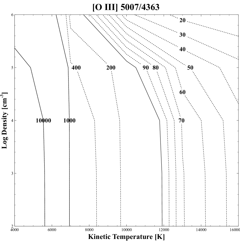
Predictions are usually saved with one of the save commands described in Hazy 1. The predictions will normally be brought together into large files which contain the output from all grid points.

0.3.6 Cloudy on parallel computers

Two Cloudy commands can take advantage of multi-core computers and high performance computing (HPC) clusters. These are the optimize and grid commands described in Sects. 0.3.4 and 0.3.5. They run Cloudy as an “embarrassingly parallel” application, putting one model on each CPU core. Run this way, the code can achieve nearly 100% efficient use of parallel computers.

The parallelization is implemented using two different techniques. The oldest technique uses the fork system call that is available under all UNIX operating systems and Apple Darwin. The great advantages of this technique are that no external libraries are needed (i.e. it works “out of the box”) and superior fault tolerance. All the work is done by the child processes, so even in the unlikely event of a crash the parent process can continue, preventing all work from being lost. The big disadvantage of this technique is that it will only work on shared-memory machines so that it cannot take advantage of modern HPC clusters. Currently only the optimize command uses this technique.

In view of the fact that HPC computing is moving away from shared-memory machines towards large HPC clusters, we decided to redesign the parallel infrastructure of the code. Since version C10.00 we support parallelization under MPI version 2 or newer. Both the optimize and grid commands can use this technique. The big advantage is that we can benefit from large HPC clusters, which is important for large grid calculations which can now be run as massively parallel applications. The disadvantage is that the user may need to install an MPI environment or at the very least needs to get familiar with MPI which unfortunately is not always as intuitive as we would like.

0.3.7 Building complex geometries

Clumping can be included and complex source geometries can be simulated. There are several general considerations.

There are powerful selection effects governing the formation of emission lines when a range of densities exist. You will tend to observe the highest-density regions because the emission per unit volume is proportional to the square density if the line is below its critical density (AGN3 Section 3.5). Only with a fine-tuned mix of densities, where the volume of material at each density exactly compensates for the change in emissivity, will an observer notice emission from a range of densities. Claims that a range of densities contribute to a single emission line should be met with some skepticism. This would require an amazing coincidence (Ferland, 2011).

But clumps do exist. If the clump size is small compared with the physical thickness of the region then they can be treated with a filling factor (see Osterbrock & Flather (1959) and AGN3 Section 5.9). In this case the gas is modeled as small clumps that are surrounded by vacuum or much lower-density gas. This is done by simply including the filling factor command to specify the fraction of the volume that is filled by clumps.

If the clumps are larger than the physical thickness of the line-forming region then each clump will have its own ionization structure. This is the “LOC” model of quasar emission-line clouds described by Baldwin et al. (1995) and Ferguson et al. (1997). The model is developed in several papers by the same team. In this case we compute grids of models and save the results. The spectra are then co-added using distribution functions to describe the range of cloud properties. The final spectrum depends on these distribution functions. Giammanco et al. (2004) show Cloudy calculations where optically thick clumps are present in the ISM.

In practice we normally use the grid command (S0.3.5) for this, but there are circumstances where complex changes in parameters may be needed. The program mpi.cpp in the programs directory in the code distribution computes a grid of models and extracts the predictions using MPI on a distributed memory machine.

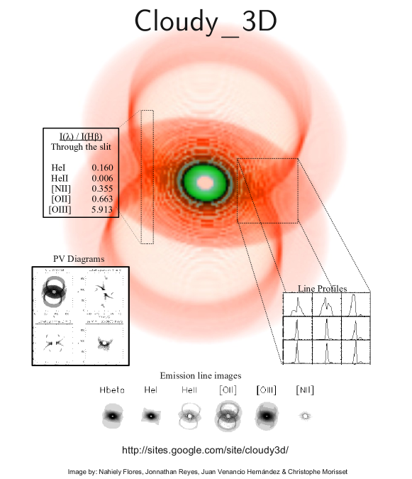
Another approach is for a driving program to use Cloudy to compute differential volume elements of a large and complex structure, and then integrate to get the next emission. An example is the Cloudy_3D code described in Morisset (2006) and Morisset & Stasinska (2008). Cloudy_3D was used to compute the image shown in Figure 3. The more recent pycloudy code by the same author is a more general tool for controlling and analyzing multiple Cloudy runs via scripts. The Rainy3D code is another example (Moraes & Diaz, 2009).

Figure 3: A 3-color image of a Hourglass-type nebula, obtained by running Cloudy_3D (Morisset, 2006). Colors are [N ii] (orange) and [O iii] (green) emission. Emission line profiles are shown for [N ii] lines. Intensities through any given slit can be obtained. Position-velocity diagrams are obtained as well as channel maps, for any line. Emission line surface brightness maps are also available for any line computed by Cloudy. Statistical tools to analyze emission-line properties are also provided.

0.3.8 Spectral energy distributions from stellar atmosphere grids

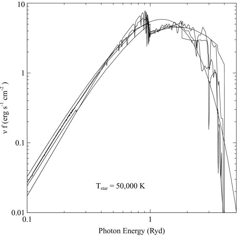
The heart of any photoionization simulation is the SED of the incident radiation field. It is this energy which is reprocessed by the cloud to produce the observed nebular emission. Several groups have created large grids of stellar SEDs using advanced stellar atmosphere codes. Other groups have used these data to create stellar population synthesis models that give the integrated spectrum of a galaxy as a function of time after a starburst. Cloudy can interpolate on SED grids having an arbitrary number of dimensions (these might include surface temperature, gravity, chemical composition, mass loss rate, age, etc) and include this in the incident radiation field.

Figure 4 compares predictions for five of the 5$\times 10^{4}$ K SEDs that are available. These include a blackbody and atmospheres computed by Mihalas (1972), Kurucz (1979), Kurucz (1991) and Rauch (2003). All were normalized to have the same total luminosity ($10^{38}$ erg s^-1) observed from a distance of $10^{18}$ cm. Note the order of magnitude dispersion among the continua for energies around 4 Ryd. This can have a major effect on the Cloudy modeling results, showing the crucial role that the stellar SED plays.

Figure 4: This figure shows the emergent radiation field predicted by five 5$\times 10^{4}$ K stars included with the code. The smoothest is the blackbody, and the Kurucz (1991) and Rauch (1997) atmospheres show the most structure.

Numerous stellar grids can be used with little additional work. In some cases the SED data are stored on the author’s web site while in others they are stored on the Cloudy web site. A convenient page providing links to all the necessary files can be found at wiki.nublado.org/wiki/StellarAtmospheres. This web page also gives more computational details and links to the papers describing the grids.

These are the most important SED grids currently supported by Cloudy:

1. The Atlas grids. There are two versions of these, the preferred one being the new-ODF grids described in Castelli & Kurucz (2004). The older generation of Atlas model atmospheres described in Kurucz (1991) is also supported. These grids can be useful if you need models for extreme metalicities not covered by the new-ODF grids. Both grids contain LTE, plane-parallel, hydrostatic model atmospheres with effective temperatures ranging between 3 500 and 50 000 K.

2. The Tlusty OSTAR2002 and BSTAR2006 grids described in Lanz & Hubeny (2003) and Lanz & Hubeny (2007). These grids contain non-LTE, line-blanketed, plane-parallel, hydrostatic O and B star SEDs. We also support merged OSTAR2002/BSTAR2006 grids covering a temperature range between 15 000 and 55 000 K.

3. The WMbasic and CoStar O and B star grids. These are two small grids of non-LTE, line-blanketed, and wind-blanketed models. The first grid is described in Pauldrach et al. (2001) and the second in Schaerer & de Koter (1997).

4. All PN central star SED grids computed by T. Rauch. These include the H-Ni, PG 1159, and C/O white dwarf grids, as well as the pure hydrogen, pure helium and H+He grids. The older H-Ca grids are also supported, though for most purposes they have been superseded by the H-Ni grids (unless you need models with T${}_{\rm eff}>$ 190 000 K). All grids contain non-LTE, line-blanketed, plane-parallel, hydrostatic model atmospheres. They are described in Rauch (1997) and Rauch (2003). The temperature range typically is between 50 000 and 190 000 K, though some grids have a different range.

5. Stellar population synthesis models from Starburst99 (Leitherer et al., 1999) and PopStar (Mollá et al., 2009). Typically the user will do their own run and generate a Cloudy grid from the output using either Cloudy commands (Starburst99) or a script supplied on the Cloudy web site (PopStar).

Many of the grids are very large and accessing them as ASCII files would be slow. They are “compiled” to create direct access binary files as part of the installation procedure. Once complete the stellar SEDs can then be accessed with the appropriate command in the simulation control deck. Logarithmic interpolation is done to create model atmospheres with any set of specified parameters using nearby models from the original grid.

The code is very flexible and allows users to create their own SED grids, e.g., from a Starburst99 run. As a result we can also add support for new grids during a release cycle when the need arises. This is possible because no code changes are needed to do this.

0.3.9 Citing Cloudy and its underlying databases

Cloudy is a research project that involves the creative efforts of many people. When used in publications it should be cited as follows: “Calculations were performed with version C13.00 of Cloudy, last described by Ferland et al. (2013)”, where this paper is the reference. The specific version of the code, written as C13.00 in this example, should be given so that, in case any future questions arise, it will be possible to reproduce the calculation using the archived versions on www.nublado.org.

We are now moving the atomic and molecular data to external databases. These are replacing our internal database, which had been embedded in the source. Many recombination coefficients are based on Badnell et al. (2003) and Badnell (2006) and posted on the web sites http://amdpp.phys.strath.ac.uk/tamoc/RR/ and http://amdpp.phys.strath.ac.uk/tamoc/DR/. Much of the molecular emission data is from LAMDA (Schöier et al., 2005) as accessed on Dec. 18, 2010, as well as the JPL (Pickett et al., 1998) and CDMS (Müller et al., 2001, 2005) databases. Much of the ionic emission data is from CHIANTI, as described by Dere et al. (1997) and Landi et al. (2012), using version 7.0. Much of the H₂ data is from Wrathmall et al. (2007), Abgrall et al. (1994), and the Meudon web site (http://molat.obspm.fr/index.php?page=pages/Molecules/H2/H2can94.php).

All of these databases play a major role in most calculations. We ask that users cite both Cloudy itself, and those underlying databases, in any publications. These databases can only thrive if their role is properly acknowledged. We provide a print citations command that will provide the correct citations in a format that can be easily copied and pasted into papers.

0.4 Applications

0.4.1 XDRs

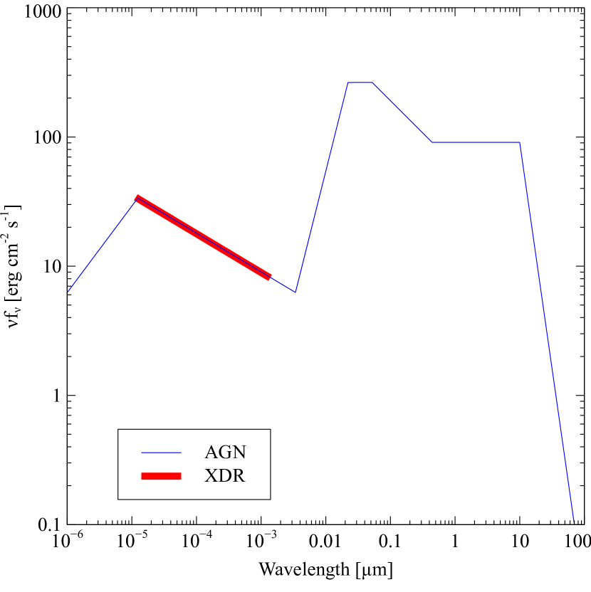
The term X-ray Dissociation Region or “XDR” was coined by Maloney et al. (1996) to describe atomic regions near X-ray sources. (A somewhat similar calculation had been presented by Ferland et al. (1994) in the context of optical filaments in cool-core clusters of galaxies.) In keeping with traditions established in the study of PDRs, a truncated SED, including only photons between 1 – 100  keV, was considered. Figure 5 shows the Maloney et al. (1996) X-ray continuum together with the mean AGN SED derived by Mathews & Ferland (1987). Both SEDs are built into Cloudy.

Figure 5: The thin line shows a mean AGN SED as deduced by Mathews & Ferland (1987). The thick line shows the truncated SED considered in XDR calculations. Both SEDs are built into Cloudy and were normalized to have the same X-ray flux.

A second Leiden meeting on radiatively excited atomic and molecular regions was held in 2012. The meeting considered five PDR and four XDR simulations. The web site gives some details along with results of the participating codes. We agreed with the PDR results, to within the considerable scatter, as had been found by Röllig et al. (2007) and Abel et al. (2008). However we systematically found less CO in the XDR simulations, as shown in the plots posted on the web site. We eventually traced this down to the cloud thickness which had not been specified for the XDR sims. Marcus Röllig kindly provided us with results submitted by other participants, and we have recomputed the XDR sims with a total hydrogen column density of $N(\textrm{H})=3\times 10^{24}\mbox{${\rm\thinspace cm}^{-2}\,$}$.

In this section we consider some details of our treatment of XDRs, since we have never directly considered such simulations before. Although our final results are within the substantial scatter of the results presented at the meeting, there are some interesting aspects of the calculation which we discuss next.

Here we consider the XDR2 test in some detail. This simulation has a hydrogen density of $n_{\rm H}=10^{3}{\rm\thinspace cm^{-3}}$, the hydrogen column density given above (corresponding to point-source A_V $\sim 10^{3}$ mag) and an X-ray flux of 270 ${\rm\thinspace erg}{\rm\thinspace cm}^{-2}{\rm\thinspace s}^{-1}\,$. The gas ionization is proportional to the dimensionless ionization parameter

$$U=\frac{\phi({\rm H})}{c\ n({\rm H})}$$ (1)

where $\phi({\rm H})$ is the flux of hydrogen ionizing photons (Osterbrock & Ferland, 2006). This simulation has the highest ionization parameter of the XDR tests, and so is one where our detailed treatment of singly and doubly charged ions makes a difference.

Photoionization by the incident radiation field, and by diffuse EUV line emission, emission lines produced by the XDR gas, produces a moderate level of ionization throughout the XDR2 cloud. Figure 6 shows the ionization fractions for H, He, and C as a function of the point-source A_V. There are significant amounts of doubly ionized species. The most important of the ions shown is He⁺, which destroys CO by charge exchange.

Figure 6: The ionization fractions for H, He, and C are shown as a function of depth, expressed as the point-source A_V.

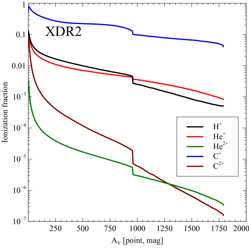
Figure 7 shows a representation of the internal radiation field at a depth corresponding to A_V = 5 mag. Although this is a shallow depth for an XDR, it is also where the warm gas that is most efficient in producing emission is found. The lower panel shows the absorption and scattering opacities, where the latter includes the factor $(1-g)$ which discounts forward scattering. Grains are the major contributor to the total scattering across the UV and optical, with Thomson scattering being dominant at the shortest and longest wavelengths. H 1 Rayleigh scattering is responsible for the feature at $\sim 0.1216\hbox{$\mu$m}$.

Grains are the dominant absorption opacity source across the UV, optical, and IR, with several resonant features visible. Below 0.0912 $\mu$m gas opacity dominates, with the strongest edge due to H⁰. Edges due to He and inner shells of the heavy elements are visible at shorter wavelengths.

The upper panel shows the local photon interaction rate, $\phi_{\nu}\alpha_{\nu}$, where $\alpha_{\nu}$ is the gas opacity [${\rm\thinspace cm}^{-2}\,$]. The local photon flux $\phi_{\nu}=4\pi\bar{J}/h\nu$ [${\rm\thinspace cm}^{-2}\,{\rm\thinspace s}^{-1}\,$] includes all components of the radiation field at that point, including the attenuated incident SED and the local diffuse line and continuous emission. The strong lines in the FUV and EUV are the result of the solution of the many-level iso-sequence atoms as described in previous sections, and have intensities that are fully self consistent with the opacities shown in the lower panel, the level of ionization, gas temperature, and optical depths. There are significant sources of ionizing radiation in addition to the attenuated incident XDR continuum. The most important are EUV recombination lines of He 1 and He 2. Direct photoionization by the incident continuum produces a trace amount of He²⁺ while the EUV emission lines, together with the incident continuum, produce a moderate amount of He⁺ and H⁺.

Figure 7: Components of the radiation field at a depth corresponding to A_V = 5 mag in the XDR2 simulation. The lower panel shows the absorption and scattering opacities while the upper panel shows the photon interaction rate.

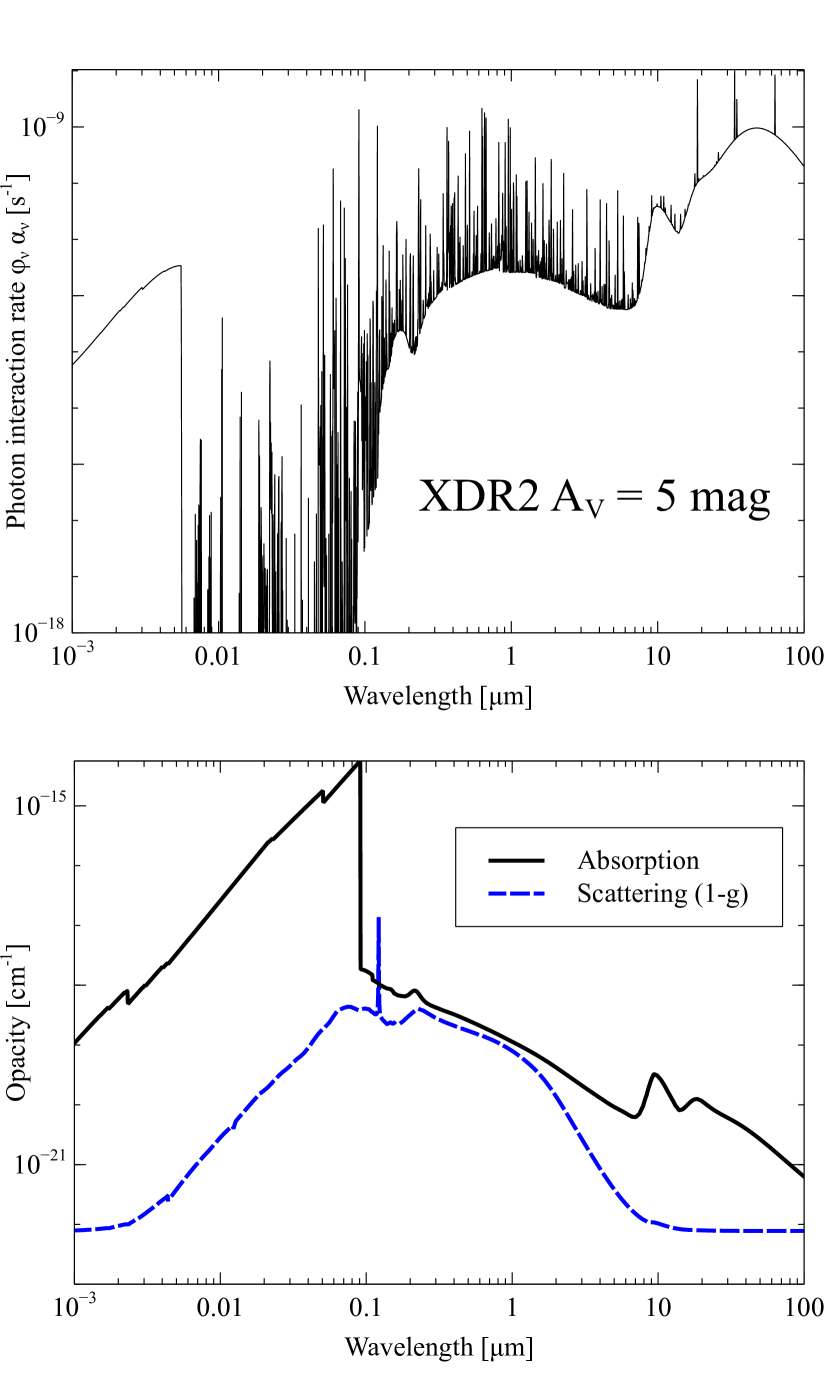
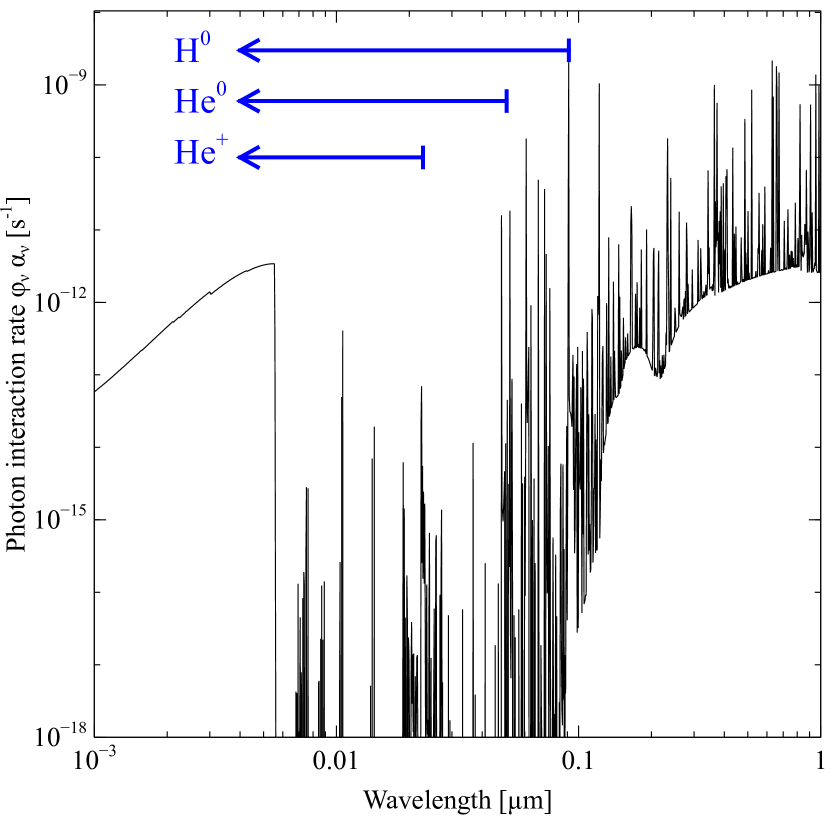
Figure 8 shows a zoom into the photon interaction rate $\phi_{\nu}\alpha_{\nu}$ within the hydrogen-ionizing radiation field. The total photoionization rate of a species is the integral of $\phi_{\nu}$ over the photoionization cross section $\sigma_{\nu}$ (AGN3), while the Figure shows the total interaction rate, evaluated using the computed total opacities. The horizontal lines indicate the range of wavelengths which can ionize H and He. For reference, photoionization cross sections fall off with decreasing wavelength as a power law ranging from $\sigma_{\nu}\sim\lambda^{-3}$ for H⁰ and He⁺ to $\sigma_{\nu}\sim\lambda^{-1}$ for He⁰. The attenuated incident XDR continuum is the dominant contributor to the He⁺ photoionization rate. Recombination lines of He 2, with a significant contribution from the XDR continuum, dominate photoionization of He⁰, and these lines, together with He I lines, ionize H⁰.

Figure 8: This shows a small portion of the radiation field around wavelengths capable of ionizing H and He. The horizontal lines indicate thresholds for photoionization of H⁰, He⁰, and He⁺.

The cumulative effect is that a significant amount of He⁺ exists across shallow parts of the cloud (Figure 6). Charge transfer between He⁺ and CO is the dominant CO destruction process in regions that are well-shielded from FUV radiation:

$${\rm He}^{+}+{\rm{CO}}\to{\rm He}+{\rm C}^{+}+{\rm O}$$ (2)

(Anicich et al., 1977; Laudenslager et al., 1974). The large amount of He⁺ results in efficient destruction of CO, and little CO exists as a result. The strong H I, He 1, and He 2 recombination lines heat the gas through both direct photoionization, and grain electron ejection.

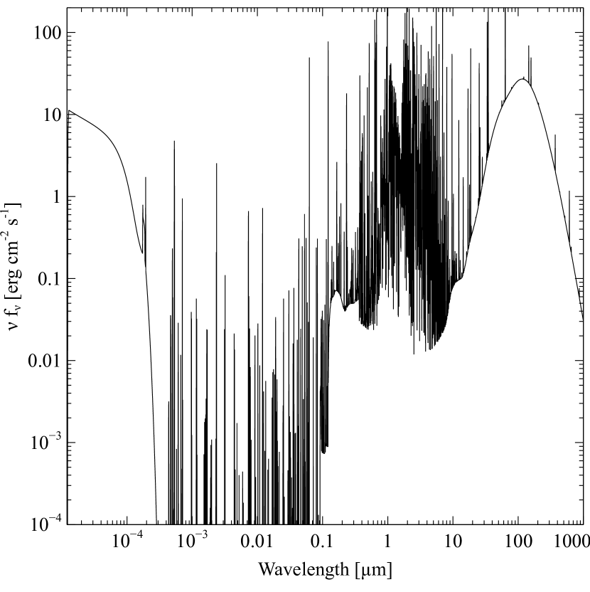
Figure 9 shows the spectrum emitted by the XDR2 cloud. The thermal infrared continuum emitted by grains, with the silicate 10 $\mu$m feature in emission, is apparent. (PAHs were not included so their features are absent.) The single strongest line is H i  L$\alpha$, produced by ionized gas present within the cloud. There is a significant amount of EUV emission at $\lambda<912$Å. The blended (at this scale) cluster of lines between $1-10\ \hbox{$\mu$m}$ is mainly produced by H₂.

Figure 9: The spectrum emergent from the XDR2 cloud. Thermal dust emission dominates in the IR while the incident XDR continuum dominates in the X-ray. A rich UV, FUX, and EUV spectrum is emitted by atoms and ions within the gas.

The goal of the 2012 Leiden workshop was to compare predictions of the CO rotation ladder. Figure 10 shows our predictions together with those of other workers, kindly provided by Marcus Röllig. Our predictions lie within range of results given by other codes, as we had previously found for PDRs Röllig et al. (2007).

Figure 10: The XDR2 CO rotation ladder predicted by codes represented at the Leiden 2012 meeting. The meeting web site gives more details.

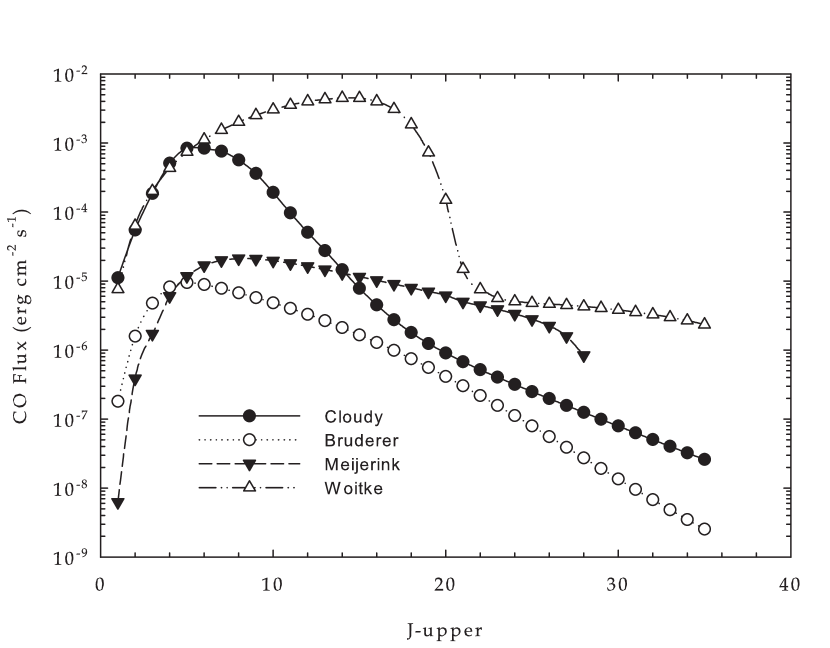
Table 1 gives the intensities of lines predicted to have emergent intensities brighter than 10% of the [C 2] $\lambda 158\hbox{$\mu$m}$ line in the format used by Cloudy. We intentionally present Table 1 in the format used by the code, as an introduction to its output. Each line is indicated by a label in the Cloudy output, given as the first column in the Table, and a wavelength, given in the second column. The line label uses the compact notation “C 2” for [C 2] so the label is intended for identification rather than spectroscopic notation. In the Cloudy output, as in Table 1, “A” and “m” indicate Å and $\mu$m respectively. A very large number of lines are predicted by Cloudy. We provide a save line labels command which will create a list of all emission lines with labels, wavelengths, and a comment indicating the line’s origin. There is a discussion of the various line entries in Part 2 of Hazy, the code’s documentation.

The third column gives the intensity, $4\pi J({\rm line})$ [${\rm\thinspace erg}{\rm\thinspace cm}^{-2}{\rm\thinspace s}^{-1}\,$] of each line. This is the total emission radiated into $4\pi{\rm\thinspace sr}$ from a unit area of cloud,

Table 1: Line intensities for XDR2 simulation

4 Spectrum Wavelength Intensitya $I/[{C\textsc{2}}]\ \lambda 158\hbox{$\mu$m}$ FeKa 1.78A $5.07\times 10^{-1}$ 5.16 H 1 1216A $1.73\times 10^{-1}$ 1.76 C 2 2326A $1.29\times 10^{-1}$ 1.32 O 2 3727A $1.34\times 10^{-2}$ 0.137 O II 3729A $1.63\times 10^{-1}$ 1.66 S 2 4074A $7.55\times 10^{-2}$ 0.768 N 1 5199A $1.66\times 10^{-2}$ 0.169 O 1 6300A $4.57\times 10^{-2}$ 0.464 O 1 6363A $1.48\times 10^{-2}$ 0.151 H 1 6563A $2.06\times 10^{-2}$ 0.209 H-CT 6563A $5.55\times 10^{-3}$ 0.056 N 2 6584A $2.16\times 10^{-2}$ 0.219 S II 6716A $1.77\times 10^{-2}$ 0.181 S II 6731A $1.43\times 10^{-2}$ 0.145 S 3 9069A $1.24\times 10^{-2}$ 0.126 S 3 9532A $3.22\times 10^{-2}$ 0.327 C 1 9850A $3.32\times 10^{-2}$ 0.338 S II 1.029m $1.34\times 10^{-2}$ 0.136 S II 1.032m $1.83\times 10^{-2}$ 0.186 S II 1.034m $1.30\times 10^{-2}$ 0.132 He 1 1.083m $2.34\times 10^{-2}$ 0.238 S 3 18.67m $9.64\times 10^{-2}$ 0.980 S 3 33.47m $3.37\times 10^{-1}$ 3.42 Si 2 34.81m $1.50\times 10^{-1}$ 1.52 O 1 63.17m $6.04\times 10^{-1}$ 6.14 O 1 145.5m $1.48\times 10^{-1}$ 1.50 C 2 157.6m $9.84\times 10^{-2}$ 1.00 C 1 369.7m $1.40\times 10^{-2}$ 0.142 TIR 1800m $1.54\times 10^{-1}$ 1.56 TALL 10000A $4.83\times 10^{+1}$ 491. aIntensity $4\pi J(\mathrm{line})$ with units ${\rm\thinspace erg}{\rm\thinspace cm}^{-2}{\rm\thinspace s}^{-1}\,$

Several lines deserve special mention. “FeKa 1.78A” is the Fe K$\alpha$ X-ray line and is mainly produced by Fe locked in silicate grains. The H$\alpha$ line is predicted to have a significant contribution by mutual neutralization excitation, indicated by the label “H-CT”. This is the process

$${\rm H}^{-}+{\rm{p}}\to{\rm H}^{*}(n=3)+{\rm H}(1s)$$ (3)

(Peart et al., 1985; Ferland & Persson, 1989). We assume that $n=3$ is statistically populated.

The last two entries represent a few of the “bands” we report. These are integrals of the emission, lines and continuum, over specified wavelength bounds. The bands can be changed by the user by editing the file continuum_bands.ini. Currently the integrated emission is reported, which is equivalent to assuming a uniform instrumental sensitivity. A number of bands, corresponding to a number of the more widely used filter or spacecraft instrumental bands, are reported. The two listed are “TIR 1800m”, the integral from 500 $\mu$m to 3100 $\mu$m, and “TALL 10000A”, the integral from 1$\times 10^{-6}$ $\mu$m to 1$\times 10^{4}$ $\mu$m.

0.4.2 XDRs and AGN

Figure 5 shows that the XDR continuum is but a small part of the total SED of an AGN. The lighter line is the mean AGN SED derived by Mathews & Ferland (1987) and built into Cloudy. The XDR SED is meant as a way to compute the conditions in the H⁰ region that lies behind (as seen from the central object) the H⁺ region where most hydrogen-ionizing radiation is absorbed. As Abel et al. (2005) stress, this may be a great oversimplification.

To check this, we computed two models of a “Narrow Lined Region” (NLR) cloud near an AGN. These are lower-density dusty regions that contribute to the optical spectrum and are likely to be ionized layers on the surface of larger molecular clouds (AGN3). Many different sets of chemical abundances are built into Cloudy. We use a standard ISM gas-phase composition and a mixture of graphite and silicate grains combined with an MRN size distribution. The clouds have a physical thickness corresponding to a column density of $N(\textrm{H})=3\times 10^{24}\mbox{${\rm\thinspace cm}^{-2}\,$}$, for a point-source A_V of $\sim 10^{3}$ mag. Galactic background cosmic rays were assumed. We now adopt the Indriolo et al. (2007) mean H⁰ cosmic ray ionization rate of $2\times 10^{-16}{\rm\thinspace s^{-1}}$ as the default Galactic background.

The AGN radiation field intensity was set with the dimensionless ionization parameter $U$, defined as the ratio of hydrogen-ionizing photon to hydrogen densities (AGN3). We adopt $\log U=-1.5$, a typical value deduced from the optical emission line spectrum (Ferguson et al., 1997). We normalized the XDR continuum to have the same 1 - 100  keV flux, 83.18 ${\rm\thinspace erg}{\rm\thinspace cm}^{-2}{\rm\thinspace s}^{-1}\,$, as the AGN continuum. The hope is that an XDR computed with this SED and flux would be similar to the H⁰ region in the AGN cloud.

The equation of state relates the gas density to other physical quantities such as the kinetic temperature or radiation pressure (see Section 0.2.8 above). We assume constant total pressure. This is very important for the AGN continuum which produces a hot ($\sim 1\times 10^{4}{\rm\thinspace K}$) layer of ionized gas on the surface of the cloud. The illuminated face of the XDR cloud is predominantly atomic and warm ($\sim 1\times 10^{3}{\rm\thinspace K}$)). As a result, for a given total hydrogen density the gas pressures will differ by about 2 dex, the difference in temperature and particle density. We want the densities in the H⁰ region to be comparable if we are to make a meaningful comparison between the two simulations. The pressure in the AGN simulation is 5.97$\times 10^{-8}$ ${\rm\thinspace g}\,{\rm\thinspace cm}^{-1}\,{\rm\thinspace s}^{-2}\,$. We use the same pressure in the XDR. The hydrogen density and temperature at the illuminated faces of the AGN and XDR clouds is then $10^{4}{\rm\thinspace cm^{-3}}$, $1.88\times 10^{4}{\rm\thinspace K}$ and $2.33\times 10^{6}{\rm\thinspace cm^{-3}}$, $2.29\times 10^{2}{\rm\thinspace K}$ respectively. Hydrogen in the AGN is fully ionized at this point while the XDR has 29% H₂.

Figure 11 shows the gas kinetic temperature and Figure 12 shows the hydrogen density as a function of depth from the illuminated face of the layer for the two scenarios. Depth is shown in terms of the point-source A_V to be consistent with other literature. Figure 13 shows the distribution of hydrogen in its various forms.

Figure 11: This compares the gas kinetic temperature for XDR and AGN clouds with the same X-ray flux, the SEDs shown in Figure 5, and the same total pressure.

Figure 12: The hydrogen density is shown for the XDR and AGN clouds.

Figure 13: The hydrogen atomic, molecular, and ion fractions are shown for the XDR and AGN clouds.

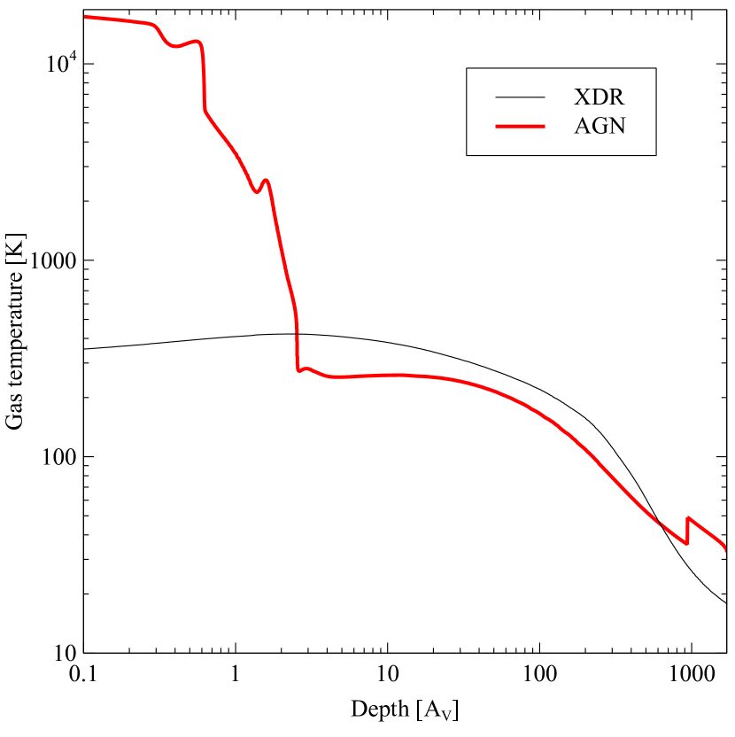
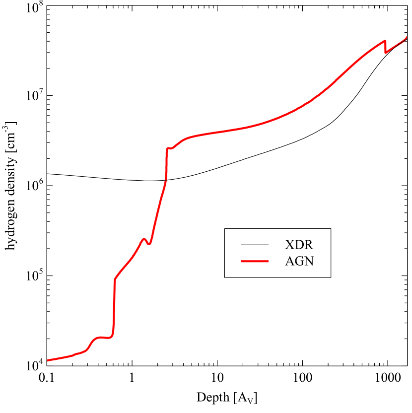
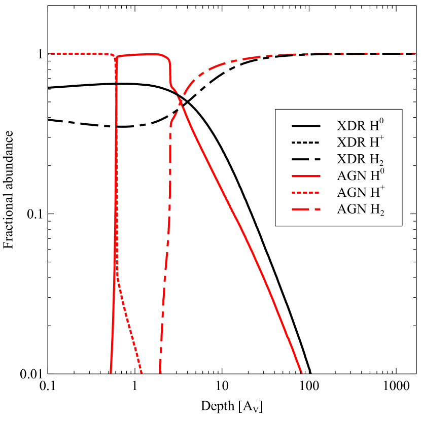
There is a very warm ionized layer in the AGN case due to the H⁺ zone where hydrogen-ionizing photons are absorbed. This layer produces most of the emission from the cloud since the AGN SED peaks in the FUV and EUV. This emission, predominantly lines in the optical and UV, may be undetectable if there is a large amount of surrounding dusty material. The UV/optical emission would then be reprocessed by other clouds into IR emission. In either case, the XDR continuum misses the majority of the continuum available for reprocessing. We shall predict the emission emergent from the cloud we model, and do not consider further reprocessing by other clouds in the system.

There are surprising large differences in the kinetic temperature in relatively shallow regions of the H⁰ region, which begins at about A_V $\sim 1$. The XDR produces a very flat temperature profile with $T\sim 300-400{\rm\thinspace K}$ being typical. The AGN produces a much warmer H⁰  layer at shallow depths with temperatures ranging from $T\sim 3000{\rm\thinspace K}$ to $T\sim 200{\rm\thinspace K}$. Soft X-rays that filter through the H⁺ layer into the H⁰ regions produce the warm gas.

Figure 14 shows the photon interaction rate at a depth of A_V$=1.5$, the region where the temperature differences between the H⁰ regions of the XDR and AGN simulations are the largest. Roughly the same amount of energy is present in the region of the spectrum where the XDR incident continuum is defined, $1-100{\rm\thinspace keV}$, although the transmitted AGN SED extends down to lower energies. This spectral region adds additional heating to the gas. The greatest differences are at $\lambda>0.1\hbox{$\mu$m}$, where $\phi_{\nu}\alpha_{\nu}$ is about 3 dex larger in the AGN simulation. This radiation heats the gas through grain electron photoejection, producing the much higher temperature.

Figure 14: The photon interaction rate at A_V$=1.5$ is shown for the XDR and AGN simulations. This is the point where the AGN has a much warmer H⁰ region, produced by the emission from the adjacent H⁺ region.

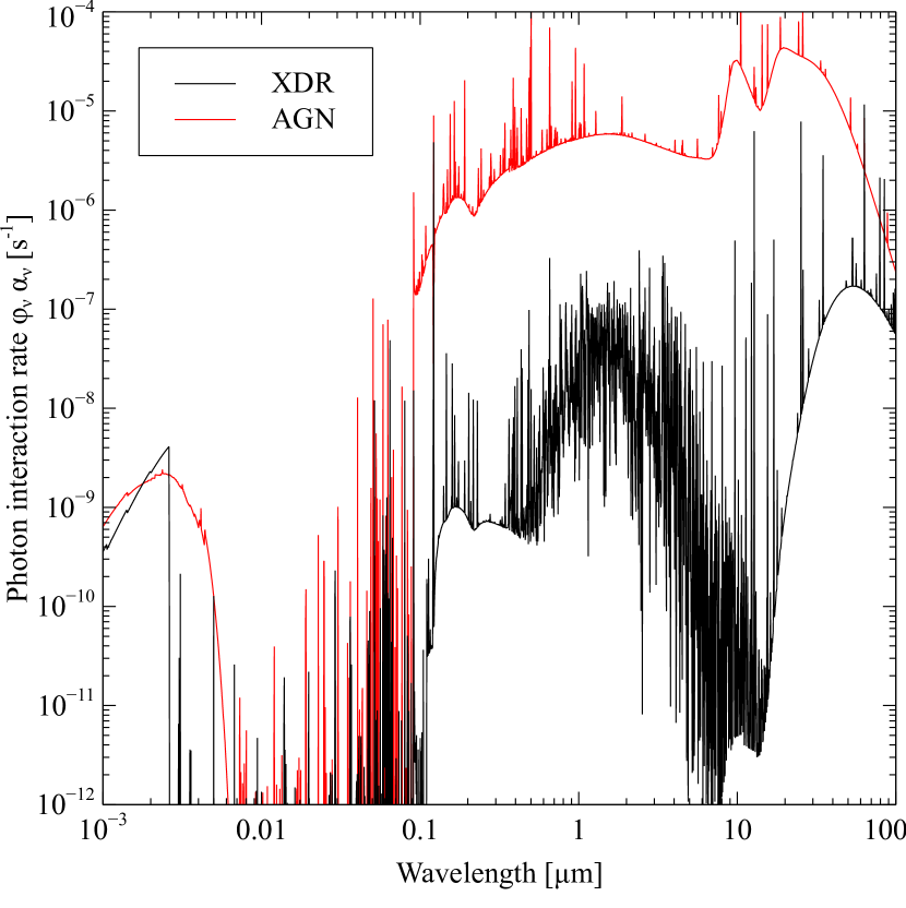
Table 2 compares predicted intensities for the XDR and AGN simulations. The XDR approximation does roughly agree with the AGN case for some MIR lines. Standard XDR emission lines such as [C ii], [O i], etc, are generally within factors of $0.3-0.5$ dex of one another. Lines from higher ionization species, such as [Ne iii] and [S iii] are bright in the AGN but missing from the XDR due to the assumed SED. The AGN produces far more total power since an AGN SED peaks at energies that are not included in a standard XDR calculation.

Table 2: Line intensities for XDR & AGN simulations

3 Line AGNa XDRa H 1 6563A $2.76$ $4.24\times 10^{-3}$ H 1 4861A $8.61\times 10^{-1}$ $1.01\times 10^{-3}$ H 1 1.875m $3.44\times 10^{-1}$ $3.85\times 10^{-4}$ O 2 3727A $1.93\times 10^{-1}$ $1.34\times 10^{-7}$ O 3 5007A $9.99$ N 2 6584A $3.67\times 10^{-1}$ S 2 6720A $5.62\times 10^{-1}$ $6.66\times 10^{-21}$ H2 2.121m $4.72\times 10^{-3}$ $4.16\times 10^{-3}$ H2 17.03m $2.20\times 10^{-2}$ $5.15\times 10^{-2}$ H2 12.28m $4.92\times 10^{-3}$ $2.40\times 10^{-2}$ H2 9.662m $2.68\times 10^{-3}$ $2.32\times 10^{-2}$ C 1 609.2m $1.03\times 10^{-4}$ $1.80\times 10^{-4}$ C 1 369.7m $5.61\times 10^{-4}$ $9.64\times 10^{-4}$ C 2 157.6m $9.48\times 10^{-3}$ $3.69\times 10^{-3}$ NE 2 12.81m $6.15\times 10^{-1}$ $2.51\times 10^{-1}$ NE 3 15.55m $1.35$ $2.99\times 10^{-3}$ SI 2 34.81m $1.34\times 10^{-1}$ $1.82\times 10^{-1}$ S 3 18.67m $6.60\times 10^{-1}$ $1.69\times 10^{-7}$ FE 2 1.644m $5.15\times 10^{-3}$ $1.53\times 10^{-13}$ C 1 609.2m $5.48\times 10^{-5}$ $8.54\times 10^{-5}$ C 1 369.7m $3.83\times 10^{-4}$ $6.26\times 10^{-4}$ C 2 157.6m $1.41\times 10^{-2}$ $3.37\times 10^{-3}$ O 1 63.17m $5.65\times 10^{-1}$ $2.51\times 10^{-1}$ O 1 145.5m $2.71\times 10^{-2}$ $1.83\times 10^{-2}$ Ne 2 12.81m $8.83\times 10^{-1}$ $3.07\times 10^{-1}$ Ne 3 15.55m $2.46$ $3.53\times 10^{-3}$ Ne 3 36.01m $1.66\times 10^{-1}$ $1.17\times 10^{-4}$ a${\rm\thinspace erg}{\rm\thinspace cm}^{-2}{\rm\thinspace s}^{-1}\,$

H₂ excitation diagrams are often used to probe physical conditions in warm molecular regions. Figure 15 shows this diagram for the two models. The overall distribution of higher populations, with $T_{exc}>4000{\rm\thinspace K}$, are similar. Lower populations indicate cooler gas for the XDR, as suggested by Figure 11. As is typical for such diagrams, lower levels, which can be excited by cooler gas, indicate lower temperatures than the high levels, which are only excited in warmer regions or by continuum pumping. The populations below 2000  K have a $\sim 250{\rm\thinspace K}$ Boltzmann distribution for the XDR, a temperature something like that of the H₂ region in Figure 13.

Figure 15: H₂ excitation diagram. The x-axis is the excitation energy of the v,J levels expressed in  K. The y-axis is the predicted column density of the v,J level divided by its statistical weight. The lines indicate thermal distributions at various temperatures.

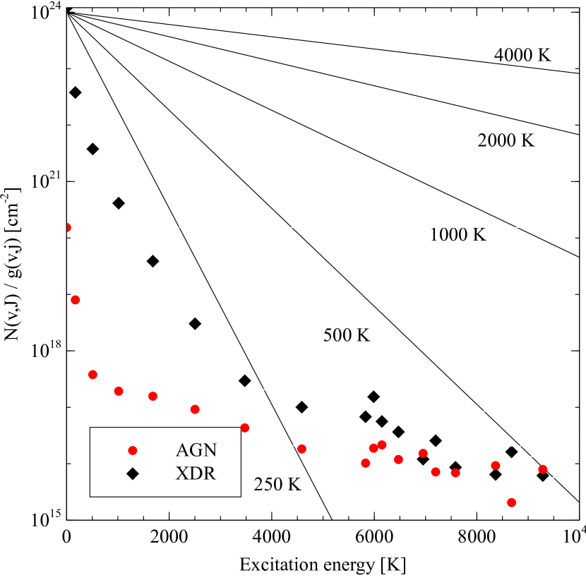
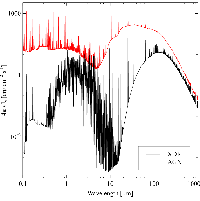
Figure 16 compares the XDR and AGN emergent spectra. The XDR is a strong source of molecular emission, filling wavelengths longward of $\sim 100\hbox{$\mu$m}$. The large “bump” of emission between $\sim 1-10\hbox{$\mu$m}$ is largely produced by H₂ lines. Molecules are prominent since little UV light is present to dissociate them, as shown in Figure 14. The AGN produces strong optical emission due to the warm H⁺ layer, and atomic and ionic emission in the IR. The dust emission is considerably warmer in the AGN case due to heating by the UV and optical radiation field.

Figure 16: The spectra emitted by the XDR and AGN simulations are shown.

0.4.3 Physical conditions over an extreme range of matter and photon density

The two previous sections highlight the types of physics that has been a particular emphasis in the code’s development since F98, dusty atomic and molecular regions. Cloudy is designed to faithfully simulate physical processes that occur in the full range of density and temperature encountered in interstellar clouds, accretion disks, or dense accretion flows. To demonstrate this range we computed (using the grid command described above) the properties of a unit cell of a photoionized cloud over a very wide range of density and intensity of the incident radiation field. Such tests are important because they show that predictions agree with analytical theory for asymptotic limiting cases.

The gas has solar composition (without grains) and is illuminated by a blackbody with a $T_{BB}=10^{6}$ K color temperature but with a variable intensity. The hydrogen density ranges from $10^{-8}{\rm\thinspace cm^{-3}}$, below that of the IGM, to $10^{18}{\rm\thinspace cm^{-3}}$, a density that is typical of the atmospheres of some stars or accretion disks. The horizontal axis is the intensity of the black body given as the energy-density temperature, $T_{u}=(u/a)^{1/4}$ K, where $u$ is the total energy density in all wavelengths [erg cm^-3] and $a$ is the Stefan radiation-density constant. This range in $T_{u}$ includes environments extending from the Intergalactic Medium (IGM) to deep layers within a star. Most clouds encountered in astrophysics have a gas and energy density that lies somewhere in Figure 17.

Figure 17: The physical properties of an irradiated cell of gas are is shown across a wide range of gas density and radiation field intensity. The upper left panel shows the log of the kinetic temperature as a function of gas density (the vertical axis) and the energy density of the radiation field (the horizontal axis). The other three panels show logs of the hydrogen molecular fraction, $2n(\mbox{{\rm H}${}_{2}$})/n({\rm H})$, and atomic and ion fraction.

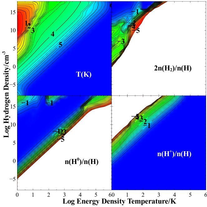
The upper left panel of Figure 17 shows the predicted gas kinetic temperature. This ranges from low values typical of cold molecular gas (the upper left-hand corner of the figure) to high values in the highly ionized right end. The gas temperature closely approaches $T_{BB}$ as $T_{u}\rightarrow T_{BB}$, as it must from thermodynamics. The right edge of the Figure corresponds to a radiation field in strict thermodynamic equilibrium (STE) since $T_{u}=T_{color}$. There is no lower bound to the gas kinetic temperature but we do see that generally $T_{kin}>T_{u}$ since the gas is not a perfect radiator. The lowest temperatures occur for the denser gas at the lowest $T_{u}$.

The remaining panels of Figure 17 show the state of hydrogen. Only fractions $n(X)/n({\rm H})>10^{-5}$ are plotted for simplicity. Bands of constant ionization parameter $U$ are the diagonals running from lower left to upper right. The gas is highly ionized in the lower right half high-$U$ region. Moving to lower $U$, going from the lower right corner towards the upper left, the gas becomes first atomic then molecular. In low-$U$ molecular regions the chemistry occurs totally in the gas phase since grains are not present.

Figure 18 is an annotated version of Figure 17 summarizing some physical limits and showing locations of some astronomical objects. This Figure is meant to illustrate the physics occurring in various combinations of density and radiation field, and is not meant to be rigorous.

Gas in the high-density region of the Figure will be in local thermodynamic equilibrium, LTE, (Mihalas, 1978; Rutten, 2003) when the density is high enough for thermal collisions to control the ionization and level populations. Levels are said to be in LTE if their level populations are given by Boltzmann statistics for the local gas kinetic temperature. The radiation field may, or may not, be a black body at this temperature. Notice that only some levels of an ion may be in LTE. In general higher electronic levels come into LTE at low densities, because of larger collision cross sections and lower transition probabilities. In C13 only ions of the H- and He-like iso-sequences have enough high levels to go to LTE. Higher densities are needed to go to LTE at larger $T_{u}$ for two reasons. Both the level of ionization and the illuminating radiation field increase with increasing $T_{u}$. Higher densities are needed if collisions are to dominate rates for level populations.

Figure 18: This panel identifies some physical and thermodynamic limits (in white) and shows where some regions in Active Galactic Nuclei are located (in yellow), for the calculations shown in Figure 17. A wide range of densities, and various energy-density temperatures of the $10^{6}{\rm\thinspace K}$ blackbody, are shown.

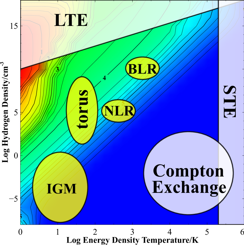
The gas is said to be in strict thermodynamic equilibrium (STE) when the ionization, level populations, and radiation field are given by the same temperature. This occurs at the right edge of Figure 18, where $T_{u}\rightarrow T_{BB}$. Our test suite includes many cases confirming that predictions go to the LTE and STE limits where expected.

The temperature in the lower-right quadrant is determined by Compton energy exchange (Ferland & Rees, 1988), which drives $T_{kin}\rightarrow T_{BB}$. Here photon - electron collisions dominate the energy exchange and the gas temperature approaches a value determined by the SED of the radiation field. Compton exchange dominates when there is little absorption opacity, which is true for the highest-$U$ regions in the lower right of the diagram.

Classical Strömgren photoionization (AGN3) operates in the mid-$T_{u}$, low to mid density, regions of the Figure. Here the approximation that most atoms are in the ground state and that all recombinations eventually reach ground (the equivalent two-level atom) is valid.

Grains tend to equilibrate at temperatures near $T_{u}$ and have sublimation temperatures around $1-1.5\times 10^{3}{\rm\thinspace K}$. They can only exist in the left third of the diagram.

Figure 18 shows where some of the emission-line regions of Active Galactic Nuclei (AGN) are located. The narrow-lined region (NLR) may be molecular clouds irradiated by the radiation field of the AGN. The BLR, likely the skin of an accretion disk near the supermassive black hole, lies between the LTE and Strömgren regimes. This environment is dense enough for there to be significant populations of excited states. Photoionization and collisional ionization from these states, and the radiative transfer effects produced by their large populations, all make this a computationally challenging environment. The molecular torus, the dusty warm molecular gas that exists outside the accretion disk and creates the AGN 1 / AGN 2 distinction (AGN3), lies along the left. The intergalactic medium (IGM) has lower gas density and is illuminated by a weak radiation field.

Figures 17 and 18 show that such diverse phenomena as the IGM, AGN molecular torus, the NLR, and the BLR are simply manifestations of different regimes of atomic and molecular physics. This is the approach we take. If the microphysics is done at an elementary level the macrophysics will follow.

0.5 A look forward

The development of Cloudy continues. The goal is a true simulation of the microphysics and spectrum of gas and dust over the range of conditions shown in Figure 18. Our calculations have always been limited by processor power, and many important physical processes are at the forefront of research in atomic, molecular, or grain physics. New simulations, which will offer better insight into what happens in front of our telescopes, will be possible with faster computers, improved numerical methods, and better physical data.

The code infrastructure is being improved. We had developed our own database for physical processes, on an ad hoc basis, and embedded it within the C++ source code. This makes it very difficult to update the database as improvements or extensions occur. We are now well into moving physical data into external databases which are parsed when the code is initialized. This effort should be complete by the next release. This external database will be public, along with the rest of Cloudy.

As described in Section 0.3.6, two commands make it possible to perform a large number of simulations in parallel using MPI. This type of “embarrassingly parallel” calculation is ideal for distributed memory systems.

Shared memory systems should be easier to program and might be used to make single models faster. As described throughout this paper, a calculation simultaneously and self-consistently solves a large number of relatively modest problems. There is no “long pole in the tent” to go after in searching for tasks to make parallel. There are many cross-dependencies between the physical parameters we calculate. Just one example: to calculate the ionization structure you need to know the radiation field, but to calculate the radiation field you need to know the ionization structure. There are many more dependencies like this one, forcing us to use iterative schemes in many places. These make parallellizing the code a lot harder. Worse, the data layout in memory is often less than optimal, resulting in poor cache utilization. Some changes have been made to improve cache locality and the potential for vectorization, but more work remains to be done. The speed of calculations on modern CPU architectures is often limited by memory bandwidth rather than compute speed. We are still considering how to take better advantage of today’s multi-core processors.

To put all this in perspective, our pn_paris test case, one of the simulations from the 1985 Paris meeting, took about a minute to compute on large mainframes at the time. Today the simulation still requires about a minute, despite the astonishing increase in computer power in the past 28 years. Today’s simulation includes many more physical processes, far better emission models, and is a much more robust model of the real nebula.

The grain physics will be improved, driven by the remarkable advances from recent infrared space missions. We will include more grain surface reactions, thought to be important in forming complex molecules. Grain opacities, especially for PAHs, depend on charge and temperature and are not a constant for a particular material and size. Finally, radio emission from spinning grains can be important and is being developed.

Filaments in cool-core clusters of galaxies are thought to be excited by penetrating energetic particles from the surrounding hot intracluster medium (Ferland et al., 2009; Fabian et al., 2011). Our treatment of cosmic ray or energetic particles does not now include attenuation (Ferland & Mushotzky, 1984), which will depend on an uncertain magnetic field geometry. Theories for cosmic ray transport do exist (Padovani et al., 2009) and may be incorporated.

Tests shown in previous papers, and demonstrated in our test suite, show that species treated with our iso-sequence model go to LTE in the high radiation or particle density limits. These include all one and two-electron species. Other ions are treated assuming equivalent two-level systems, as described above, and cannot to go LTE. This is the greatest weakness in our simulations at high densities. We intend to extend the iso-sequence approach to more species, using accurate atomic databases to model lower levels. We can now use both Chianti and Stout, our new external database. Chianti does not include subordinate collisions and so cannot go to LTE. It was intended for relatively low densities. Our Stout database includes all collisions. Neither extends to high enough energy levels for collisional coupling to the continuum and LTE to occur. These models will have to be supplemented with higher Rydberg levels to allow the appropriate high-density behavior to occur.

Much work remains to be done. A true simulation of the physical state of matter over the extremes of conditions found in astrophysics is the first step in understanding the messages in the light we observe. This goal is within sight.

DEDICATION

We dedicate this paper to Manuel Peimbert. Through his leadership the traditions established by Menzel, Baker, Aller, Strömgren, Osterbrock & Seaton are being carried on, in Mexico.