Homotopic Group ICA for Multi-Subject Brain Imaging Data

Abstract

Independent Component Analysis (ICA) is a computational technique for revealing latent factors that underlie sets of measurements or signals. It has become a standard technique in functional neuroimaging. In functional neuroimaging, so called group ICA (gICA) seeks to identify and quantify networks of correlated regions across subjects. This paper reports on the development of a new group ICA approach, Homotopic Group ICA (H-gICA), for blind source separation of resting state functional magnetic resonance imaging (fMRI) data. Resting state brain functional homotopy is the similarity of spontaneous fluctuations between bilaterally symmetrically opposing regions (i.e. those symmetric with respect to the mid-sagittal plane) (Zuo et al., 2010). The approach we proposed improves network estimates by leveraging this known brain functional homotopy. H-gICA increases the potential for network discovery, effectively by averaging information across hemispheres. It is theoretically proven to be identical to standard group ICA when the true sources are both perfectly homotopic and noise-free, while simulation studies and data explorations demonstrate its benefits in the presence of noise. Moreover, compared to commonly applied group ICA algorithms, the structure of the H-gICA input data leads to significant improvement in computational efficiency. A simulation study comfirms its effectiveness in homotopic, non-homotopic and mixed settings, as well as on the landmark ADHD-200 dataset. From a relatively small subset of data, several brain networks were found including: the visual, the default mode and auditory networks, as well as others. These were shown to be more contiguous and clearly delineated than the corresponding ordinary group ICA. Finally, in addition to improving network estimation, H-gICA facilitates the investigation of functional homotopy via ICA-based networks.

Keywords: Brain Functional Homotopy, Functional MRI, Independent Component Analysis

1 Introduction

The function of the human brain during rest can be investigated using various functional measurement techniques (Biswal et al., 1995; Gusnard et al., 2001; Gao et al., 2009). Patterns of resting-state brain functional across individuals provide insights into baseline activity of the human brain in the absence of experimental stimuli.

Resting state functional magnetic resonance imaging (rs-fMRI), obtained using blood oxygen level dependent (BOLD) signals, is a key driving force for investigating baseline fluctuations in brain activity. Much recent attention has been focused on identifying the possible origins and clinical manifestations of variation in the BOLD signals from rs-fMRI data. Neuroimaging studies have identified associations between resting state brain networks estimated via fMRI data with aging, cognitive function and neurological and psychiatric disorders (Damoiseaux et al., 2008; Rombouts et al., 2005). One popular approach for locating putative networks is blind source separation, which decomposes neuroimaging data into an outer product of spatial maps multiplied by their respective time courses. Notably, blind source separation does not require a specific fMRI paradigm, so is applicable to resting state data. Two popular exploratory data analysis techniques for blind source separation are Principal Component Analysis (PCA) and Independent Component Analysis (ICA). ICA can be distinguished from PCA by its focus on model-level independence and non-Gaussianity. Moreover, ICA as a matrix decomposition does not yield decomposition vectors that are orthonormal. Finally, ICA is usually applied after PCA-based dimensional reduction, and thus can be thought of as a non-orthonormal reorganization of PCA.

ICA has become popular for analyzing neuroimaging data, having been successfully applied to single-subject analysis (Guo and Pagnoni, 2008; Beckmann and Smith, 2004; McKeown et al., 1997). The extension of ICA to group inferences provides common independent components across subjects and enables identification of putative underlying brain networks for the group. Several multi-subject ICA approaches have been proposed: Calhoun et al. (2001b) presented (and named) group ICA (gICA) and created the Matlab toolbox (GIFT), which provides estimation. GIFT consists of a first-dimension reduction using PCA for each subject, followed by a temporal concatenation of the reduced data, after which ICA is then applied to the aggregated data. More recently, Beckmann and Smith (2005) proposed a tensor ICA (TICA) by extending the single-session probabilistic ICA (PICA) (Beckmann and Smith, 2004). TICA factors the multi-subject data as a tri-linear combination of three outer products, which represents the different signals and artifacts present in the data in terms of their temporal, spatial, and subject-dependent variations. Other grouping methods proposed perform ICA on each subject and combine the output into a group by using self-organizing clustering (Esposito et al., 2005) or spatial correlation (Calhoun et al., 2001a).

Among existing methods, GIFT is perhaps the most commonly used for performing group ICA analysis of multi-subject fMRI data. The spatial independence assumed by GIFT, and any other spatial ICA algorithms, is well suited to the spatial patterns seen in fMRI (McKeown et al., 1997). Moreover, its empirical performance has been consistently validated (Sorg et al., 2007; Garrity et al., 2007; Sambataro et al., 2010).

This paper describes a novel modified group ICA method - homotopic group ICA (H-gICA) - to identify the underlying patterns of brain activity for functionally homotopic putative networks. Left to right bilaterally symmetric patterns of interhemispheric synchrony and co-activation are among the most frequent findings in neuroimaging studies (Toro et al., 2008). Functional homotopy, the similarity of spontaneous fluctuations between bilaterally symmetrically opposing regions with respect to the mid-sagittal plane is a “fundamental characteristic of the brain’s intrinsic functional architecture” (Zuo et al., 2010). Via H-gICA, the information of homotopic brain function is utilized to improve the identification of underlying brain networks. A spatial independence assumption is made relating to all voxels in each hemisphere. In a simulation study, H-gICA is shown to be preferable to (our implementation of) GIFT when the actual signals are homotopic and is competitive with GIFT under non-homotopic signal conditions. The efficacy of H-gICA methodology is demonstrated by an application to the ADHD-200 dataset (Milham, 2012; Eloyan et al., 2012). From the fifteen components produced by H-gICA, several common brain networks were found, being clearly represented in smoother, more clearly delineated and contiguous volumes than ordinary gICA. The main networks found include the visual, default mode and auditory. In addition to improving network estimation, H-gICA allows for the investigation of functional homotopy via ICA-based networks. Here the quantification of functional homotopy of such networks are defined using a similar concept to that of Joel et al. (2011). Specifically, by having left and right hemispheric terms in the model, investigations of ICA weight matrices includes homotopic information, unlike ordinary group ICA.

The remainder of the paper is organized as follows. ICA and fast, fixed-point algorithm known as FastICA proposed by (Hyvärinen, 1999) is reviewed in Section 2, and subsequently used in the estimation of H-gICA. Section 3 is the theoretical body of the paper: Section 3.1 discusses about data preprocessing issues; Section 3.2 introduces the H-gICA model; Section 3.3 proves that H-gICA and GIFT coincide under noise-free settings; and Section 3.4 provides a measure of the functional homotopy for ICA-based networks. Section 4 provides a simulation study to demonstrate the effectiveness of H-gICA under homotopic, non-homotopic and mixed settings. This allows a comparison versus GIFT, demonstrating that by using intrinsic functional homotopy of the brain, H-gICA improves the power of locating the underlying brain networks. Section 5 provides the application of the H-gICA on the ADHD-200 dataset, an open source dataset with 776 children and adolescents, while Section 6 contains a summary discussion.

2 Background

The observed data are denoted by $\mbox{\boldmath$x$}=(x_{1},x_{2},\cdots,x_{m})^{T}$, an $m$-dimensional random vector, and the true underlying signals by $\mbox{\boldmath$s$}=(s_{1},s_{2},\cdots,s_{n})^{T}$, an $n$-dimensional transform of $x$. The problem is to determine a matrix $W$ so that

$$\mbox{\boldmath$s$}=\mbox{\boldmath$W$}\mbox{\boldmath$x$}.$$ (1)

A distinguishing feature of ICA components is that the elements of $s$ are assumed to be independent in a generative factor analytic model, instead of focusing on data-level uncorrelatedness. The ICA problem can be formulated using the following generative model for the data:

$$\mbox{\boldmath$x$}=\mbox{\boldmath$A$}\mbox{\boldmath$s$},$$ (2)

where $x$ is the observed $m$-dimensional vector, $s$ is the $n$-dimensional (latent) random vector whose components are assumed mutually independent, and $A$ is a constant $m\times n$ matrix to be estimated. If it is further assumed that the dimensions of $x$ and $s$ are equal, i.e., $m=n$, the estimate of $W$ in (1) is then obtained as the inverse of the estimate for matrix $A$.

Because of the assumption that $A$ is invertible, a first stage dimension reduction is required. Thus the model can be more accurately stated as $\mbox{\boldmath$K$}\mbox{\boldmath$x$}=\mbox{\boldmath$A$}\mbox{\boldmath$s$},$ where $K$ is a dimension reduction matrix of size $n\times m$. Normally, this is reached via a singular value decomposition of the demeaned data. Henceforth, we will assume that the data vectors are $n$ dimensional. Also note that the data are typically de-meaned prior to analysis.

2.1 FastICA

The previously mentioned dimension reduced data input into an ICA algorithm are mean zero and uncorrelated, and thus Gaussian distributional assumptions provide little further insight to linear reorganizations. This, along with the idea that linearly mixed iid noise tends to appear Gaussian, has lead researchers to design algorithms that search for an optimized $W$ that maximizes non-Gaussianity. Such non-Gaussianity of the independent components is necessary for the identifiability of the model shown in Equation (2) (Comon, 1994). Two common measures of non-Gaussianity used in ICA are kurtosis (Oja et al., 2001) and negentropy (Pillai et al., 2002).

Hyvärinen (1999) proposed a fast fixed-point algorithm known as FastICA. Following Hyvarinen’s treatment of ICA, mutual information (Oja et al., 2001), a natural measure of the dependence between random variables, can be written as

$$J(\mbox{\boldmath$y$})-\sum\limits_{i}J(y_{i}),$$

when the variables $y_{i}$, $i=1,\ldots,n$, are uncorrelated. Here $\mbox{\boldmath$y$}=(y_{1},\cdots,y_{n})^{T}$ and $J$ is negentropy, a measure of non-Gaussianity (Comon, 1994). Thus, $W$ is determined so that the mutual information of the independent components, $s_{i}$, is minimized. As mentioned by Hyvärinen (1999), this is approximately equivalent to finding directions in which the negentropy is maximized.

For any random variable, $y_{i}$, with zero mean and unit variance, an approximation to the negentropy is proportional to $[E\{G(y_{i})\}-E\{G(Z)\}]^{2}$ for appropriately chosen $G$ where $Z$ is a standard normal. As an example, if $G(y)=y^{4}$, one results in ICA methods that approximate minimum kurtosis algorithms. With this approximation, it can be shown that the problem is equivalent to finding $\mbox{argmax}_{w_{i}}\sum_{i=1}^{n}J_{G}(\mbox{\boldmath$w$}_{i})\$ under the constraint that $E\{(\mbox{\boldmath$w$}_{k}^{T}\mbox{\boldmath$x$})(\mbox{\boldmath$w$}_{j}^{T}\mbox{\boldmath$x$})\}$ is $0$ with $j\neq k$ and $1$ when $j=k$. Here $J_{G}$ is given by $J_{G}(\mbox{\boldmath$w$}):=[E\{G(\mbox{\boldmath$w$}^{T}\mbox{\boldmath$x$})\}-E\{G(Z)\}]^{2}$. The FastICA algorithm that we employ uses fixed-point iterations for maximization.

2.2 Group ICA

The extension of ICA to group inferences provides common independent components across subjects, which allows identification of putative common brain networks for the whole group. As in most fMRI studies, spatial independence is assumed in our group ICA model, since it is well-suited to the sparse distributed nature of the spatial pattern for most cognitive activation paradigms (McKeown et al., 1997). However, instead of the entire brain, the spatial independence assumption in H-gICA is made for voxels within a single hemisphere. To use the information of brain functional homotopy, the fMRI data are registered to symmetric templates and thus the number of voxels are equal in the left and right hemispheres. Similarly to in Calhoun et al. (2001b), a dimension reduction using PCA is applied to each hemisphere of each subject. Another PCA step is then performed on the concatenated data matrix, which is not technically necessary (Eloyan et al., 2013) though is the current standard practice for group ICA.

3 Methods

3.1 Preprocessing

All group ICA methods for rs-fMRI require brains to be registered via a deformation algorithm to a canonical brain image, referred to as a template. This allows the assumption of spatially common brain networks elaborated on in Section 2.2. While our approach is applicable to any standard preprocessing, we do assume that the template is bilaterally symmetric along the mid-sagittal plane, contrary to all human neuroanatomy. The creation and improvement of such templates is beyond the scope of this work. However briefly, a simple strategy would require an accurate hemispheric model, a deformation to force the mid-sagittal plane to be perfectly planar, them flipping one hemisphere and pasting it together with itself to form the template. Fortunately, symmetric template brains exists; we employ one create by the International Consortium for Brain Mapping (ICBM) (Fonov et al., 2011b, 2009a). An easy solution for preprocessing is to take already processed data, registered to a non-symmetric template, and apply a second registration to a symmetric template. As such, the method can be applied to existing processed data easily. Without loss of generality, it is assumed that the mid-sagittal plane is parallel to one of the image dimensions.

3.2 Homotopic Group ICA

Homotopic group ICA is the simple idea of having each subject contribute two fMRI images, one for their left hemisphere and one for their right, to the gICA approach. The benefit of the approach is the reduction in data level noise by (effectively) doubling the number of subjects and halving the number of voxels. Furthermore, it directly utilizes the information that many brain networks are apparently bilaterally symmetric.

Suppose there are $N$ subjects indexed by $i=1,2,\ldots,N$ with an fMRI time series comprised of $T$ scans. Further, suppose that each subject’s fMRI image contains $2V$ voxels with $V$ in each hemisphere for each time point. Separate the two hemispheres with two matrices of size $T\times V$, labeled $\mbox{\boldmath$F$}_{i,1}$ and $\mbox{\boldmath$F$}_{i,2}$. Assume these have column sums zero (they are demeaned over time) and that one side has been appropriately flipped to geometrically match the other. Conceptually, let $\mbox{\boldmath$F$}_{i}(a,b,c,t)$ be a subject’s image represented as a 4D array. Here, $a$ indexes the left to right dimension where $a=1,\ldots,2K$, $b$ indexes the anterior/posterior dimension, $c$ indexes the superior/inferior dimension and $t$ indexes scan. Suppose that the mid-sagittal plane is defined as $a=K$. Then, the 4D array defined as $\mbox{\boldmath$F$}_{i}(a,b,c,t)$ for $a<K$ defines one hemisphere’s image series, while $\mbox{\boldmath$F$}_{i}(2K-a,b,c,t)$ defines the other, oriented in a geometrically similar manner. The left, $\mbox{\boldmath$F$}_{i,1}$, and right, $\mbox{\boldmath$F$}_{i,2}$, hemispheric data matrices are obtained from the associated left and right hemispheric images, having vectorized the spatial dimension.

Assume a principal component dimension reduction has been applied and, abusing notation, that $\mbox{\boldmath$X$}_{i,j}$ of size $Q\times V$ denotes the dimension reduced data matrix of the left ($j=1$) and right ($j=2$) hemispheres of subject $i$. The column $v$ of $\mbox{\boldmath$X$}_{i,j}$ continues to represent voxel $v$ in hemisphere $j$. The rows of $\mbox{\boldmath$X$}_{i,j}$ are the PCs, which are indexed by $t=1,2,\ldots,Q$.

$\mbox{\boldmath$X$}_{i,j}(t,v)$ represents row $t$, column $v$ of $\mbox{\boldmath$X$}_{i,j}$ with the same convention applied to other vectors and matrices. Assuming that a group ICA decomposition implies: $\mbox{\boldmath$X$}_{i,j}(t,v)=\sum\limits_{q=1}^{Q}\mbox{\boldmath$A$}_{i,j}(t,q)\mbox{\boldmath$S$}(q,v),$ for all $i=1,2,\ldots,N$ and $j=1,2$. This in turn implies that the spatio-temporal process $\mbox{\boldmath$X$}_{i,j}(t,v)$ can be decomposed to a hemisphere specific time series $\mbox{\boldmath$A$}_{i,j}(t,q)$ and a subject-independent spatial maps, $\mbox{\boldmath$S$}(q,v)$. This is equivalent to the following group ICA model:

$$\mbox{\boldmath$X$}=\mbox{\boldmath$M$}\mbox{\boldmath$S$}.$$ (3)

Here $\mbox{\boldmath$X$}=[\mbox{\boldmath$X$}_{1}^{T},\mbox{\boldmath$X$}_{2}^{T}]^{T}$ is the $2NQ\times V$ group data matrix from left and right hemispheres, where $\mbox{\boldmath$X$}_{j}:=[\mbox{\boldmath$X$}_{1,j}^{T},\mbox{\boldmath$X$}_{2,j}^{T},\cdots,\mbox{\boldmath$X$}_{N,j}^{T}]^{T}$, $j=1,2$, which formed by concatenating $N$ subjects’ data in the temporal domain. $S$ is $Q\times V$ matrix containing $Q$ statistically independent spatial maps in its rows. $\mbox{\boldmath$M$}=[\mbox{\boldmath$M$}_{1}^{T},\mbox{\boldmath$M$}_{2}^{T}]^{T}$ is the $2NQ\times Q$ group mixing matrix, where $\mbox{\boldmath$M$}_{j}=[\mbox{\boldmath$A$}_{1,j}^{T},\mbox{\boldmath$A$}_{2,j}^{T},\cdots,\mbox{\boldmath$A$}_{N,j}^{T}]^{T}$ is the $NQ\times Q$ submatrix corresponding to hemisphere $j$ concatenating the mixing matrix of the $N$ subjects. In the context of fMRI, the $\mbox{\boldmath$S$}(q,\cdot)$, $q=1,2,\ldots,Q$ are spatial maps that are the putative brain networks to be estimated. The mixing matrices are assumed non singular, and thus we can define $\mbox{\boldmath$W$}_{i,j}=\mbox{\boldmath$A$}_{i,j}^{-1}$.

In the H-gICA model, the independent components are assumed to be common across subjects and hemispheres, while how they mix to produce the signal can differ among both subjects and hemispheres. Of course, the true mixing matrices are not observed and the FastICA algorithm is used to obtain the estimates.

3.3 Connection with gICA

In this section H-gICA is linked to the most commonly used group ICA approach (Calhoun et al., 2001b). Let $\tilde{\mbox{\boldmath$X$}}=[\mbox{\boldmath$X$}_{1},\mbox{\boldmath$X$}_{2}]$ be the $NQ\times 2V$ dimension reduced group data matrix, where $\mbox{\boldmath$X$}_{j}=[\mbox{\boldmath$X$}_{1,j}^{T},\mbox{\boldmath$X$}_{2,j}^{T},\cdots,\mbox{\boldmath$X$}_{N,j}^{T}]^{T}$ is same as in Section 3.2. Here, we are simply pasting the hemispheric data back together. The standard gICA approach decomposes $\tilde{\mbox{\boldmath$X$}}$ as $\tilde{\mbox{\boldmath$X$}}=\tilde{\mbox{\boldmath$M$}}\tilde{\mbox{\boldmath$S$}}.$ Here, $\tilde{\mbox{\boldmath$S$}}$ is a $Q\times 2V$ matrix containing $Q$ spatial maps in its rows. And $\tilde{\mbox{\boldmath$M$}}=[\tilde{\mbox{\boldmath$A$}_{1}}^{T},\tilde{\mbox{\boldmath$A$}_{2}}^{T},\cdots,\tilde{\mbox{\boldmath$A$}_{N}}^{T}]^{T}$ is the $NQ\times Q$ group mixing matrix, where $\tilde{\mbox{\boldmath$A$}_{i}}$ is the $Q\times Q$ submatrix corresponding to subject $i$. Under the assumption that $\tilde{\mbox{\boldmath$A$}_{i}}$, are of full rank, defines $\tilde{\mbox{\boldmath$W$}_{i}}=\tilde{\mbox{\boldmath$A$}_{i}}^{-1}$, which can also be estimated by the FastICA algorithm. The following theorem, shows that if the actual sources are truly homotopic and noise free, H-gICA and gICA provide the same result when using the estimation method of FastICA. The proof of the theorem is given to the Appendix.

Theorem 3.1.

Suppose the actual sources are truly homotopic and noise free. The number of estimated ICs is $Q\ll V$. Denote the FastICA estimate of $S$ to be $\hat{\mbox{\boldmath$S$}}$ and the estimate of $\tilde{\mbox{\boldmath$S$}}$ to be $\hat{\tilde{\mbox{\boldmath$S$}}}$. Then for $j\in\{1,2\}$, we have $\hat{\tilde{\mbox{\boldmath$S$}}}=[\hat{\mbox{\boldmath$S$}},\hat{\mbox{\boldmath$S$}}].$

Theorem 3.1 shows that when there is no noise, H-gICA and GIFT are the same for the homotopic signals. However, of course, noise exists in most real data sets. Section 4 deals with H-gICA’s ability to improve locating underlying sources when noise is added to the data.

3.4 Measures of Functional Homotopy

In rs-fMRI, ICA output can be used to obtain measures of network connectivity, which are of intrinsic interest in studying neural function (Gao et al., 2012). Joel et al. (2011) point out that the functional connectivity between any two brain regions may be due to within network connectivity (WNC) and between network connectivity (BNC). They emphasize the importance of interpreting such connectivity, ostensibly measured by the correlation and variance of the temporal mixing matrices.

Similarly to Joel et al. (2011) the following defines a measure of subject- and network-specific functional homotopy for the $k^{th}$ ICA based network of subject $i$:

$$H_{i}(k)=\text{Cor}(\mbox{\boldmath$A$}_{i,1}^{(k)},\mbox{\boldmath$A$}_{i,2}^{(k)}),$$ (4)

where $\mbox{\boldmath$A$}_{i,j}$ $(i=1,2,\ldots,N,j=1,2)$ is the mixing matrix of the $i^{th}$ subject corresponding to hemisphere $j$ and $\mbox{\boldmath$A$}_{i,j}^{(k)}$ is a vector of the time course modulating spatial map $k$. Note, typically this requires a back transformation from PCA space. Here $H_{i}(k)$ measures the spontaneous activity of the $k^{th}$ network between left and right hemispheres. The estimation of $H_{i}(k)$ in H-gICA is given by replacing $\mbox{\boldmath$A$}_{i,1}$ and $\mbox{\boldmath$A$}_{i,2}$ with their estimated values in (4). Similarly the group level functional homotopy for the $k^{th}$ ICA based network can be define as:

$$H(k)=\text{Cor}(\mbox{\boldmath$M$}_{1}^{(k)},\mbox{\boldmath$M$}_{2}^{(k)}),$$ (5)

where $\mbox{\boldmath$M$}_{j}$ is defined in (3) as the submatrix corresponding to hemisphere $j$ concatenating the mixing matrix of the $N$ subjects and $\mbox{\boldmath$M$}_{j}^{(k)}$ is the $t^{th}$ element of the time course modulating spatial map $k$.

4 Simulation Results

4.1 A Simple Example

The following simple example is given to initially demonstrate the effectiveness of H-gICA. Suppose the number of subject is $N=3$ and the number of underlying sources is $Q=3$. For each subject $i$, the $T\times 2V$ data matrix $\tilde{\mbox{\boldmath$X$}}_{i,\cdot}=[\mbox{\boldmath$X$}_{i,1},\mbox{\boldmath$X$}_{i,2}]$ is from the model $\tilde{\mbox{\boldmath$X$}}_{i,\cdot}=\mbox{\boldmath$A$}_{i}\tilde{\mbox{\boldmath$S$}}$ with $T=3$ and $2V=10^{2}$. We further assume that

$$\mbox{\boldmath$A$}_{1}=\left({\begin{array}[]{*{20}c}{-1}&{-5}&{2}\\ {5}&{-3}&{2}\\ {5}&{3}&{-5}\\ \end{array}}\right),\mbox{\boldmath$A$}_{2}=\left({\begin{array}[]{*{20}c}{-1}&{-1}&{2}\\ {-1}&{-2}&{-3}\\ {-4}&{0}&{5}\\ \end{array}}\right),\mbox{\boldmath$A$}_{3}=\left({\begin{array}[]{*{20}c}{-3}&{3}&{-5}\\ {5}&{-1}&{-1}\\ {3}&{-2}&{-1}\\ \end{array}}\right)$$

(The elements in $\mbox{\boldmath$A$}_{1}$, $\mbox{\boldmath$A$}_{2}$ and $\mbox{\boldmath$A$}_{3}$ are randomly picked from $Unif(-10,10)$.)

As shown in Figure 1, three different source matrices ($\tilde{\mbox{\boldmath$S$}}$) are generated: one is symmetric; another is only in one hemisphere; and the third has two asymmetric blocks of activated voxels.

Figure 1: Result of the first example. The top row shows the true sources in three different types: perfectly symmetric; only present in one hemisphere; differing in the two hemispheres. The small blocks in these plots are activated voxels, where the values come from uniform distribution. The first two elements of the second row are the true sources in the left hemisphere and the last element is left minus right. The bottom row consists of the independent components generated by H-gICA.

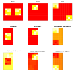
These results are shown in the bottom row of Figure 1, highlighted by H-gICA’s separation of the three source matrices and its meaningful prediction for all of them.

4.2 2D Simulation

In order to illustrate the performance of the proposed method, simulation studies with $10,000$ voxels in 2D spaces were conducted. Both the homotopic and non-homotopic settings are used in the study. The results are compared with the commonly used group ICA algorithm without consideration of the left and right hemispheres.

Similar to above, the number of subjects is $N=3$ and the number of underlying sources is $Q=3$. The data are generated by the ICA model $\tilde{\mbox{\boldmath$X$}}_{i,\cdot}=\mbox{\boldmath$A$}_{i}\tilde{\mbox{\boldmath$S$}}$ with $T=3$ and $2V=100^{2}$. $\mbox{\boldmath$A$}_{i}$ has the same value as in the toy example for $i=1,2,3$ is also assumed.

4.2.1 Case I: Perfect Homotopy

Assume all true sources are perfectly homotopic. For each source, two blocks of voxels are symmetrically activated. In each loop of the simulation, values of these activated voxels are assigned by Gamma distributions. The heatplots of the sources are shown in Figure 2.

Figure 2: True Sources in the Perfect Homotopy. The three sources are generated by Gamma distributions with different parameters.

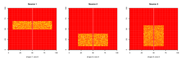
The data are generated by the three sources in Figure 2 and the mixing matrices $\mbox{\boldmath$A$}_{1}$, $\mbox{\boldmath$A$}_{2}$, and $\mbox{\boldmath$A$}_{3}$. Gaussian noise is then added to the data. The estimated components are standardized and subsequently compared with the corresponding standardized true sources. Next, the mean difference at each voxel is calculated. The simulation contained 300 iterations in each run. Homotopic gICA results are compared with the commonly used group ICA algorithm in Table 1, where the noise is set to be mean zero and with a standard deviation equal to $5$.

Table 1: The two rows compare the mean of the voxel mean difference of H-gICA and ordinary gICA in the symmetric setting.

	Source 1	Source 2	Source 3
H-gICA	0.414 ($\sim 0.001$)	0.412 ($\sim 0.001$)	0.423 ($\sim 0.002$)
gICA	0.507 ($\sim 0.001$)	0.496 ($\sim 0.001$)	0.433 ($\sim 0.001$)

As seen in Table 1, in the setting of symmetric sources, the mean errors of H-gICA are smaller than that of ordinary gICA for all the three sources. Figure 3 shows the mean of the voxel mean difference with different settings for the noise. Again, H-gICA works consistently better when noise exists and is the same as ordinary gICA in noise-free settings, which was been proven in Theorem 3.1.

Figure 3: The mean of the voxel mean difference increases with the standard deviation of the noise. The two methods are the same under noise-free settings and when the noise exists, H-gICA works better than ordinary gICA.

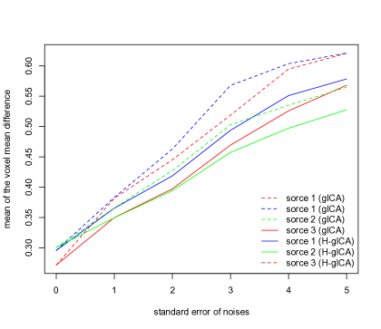
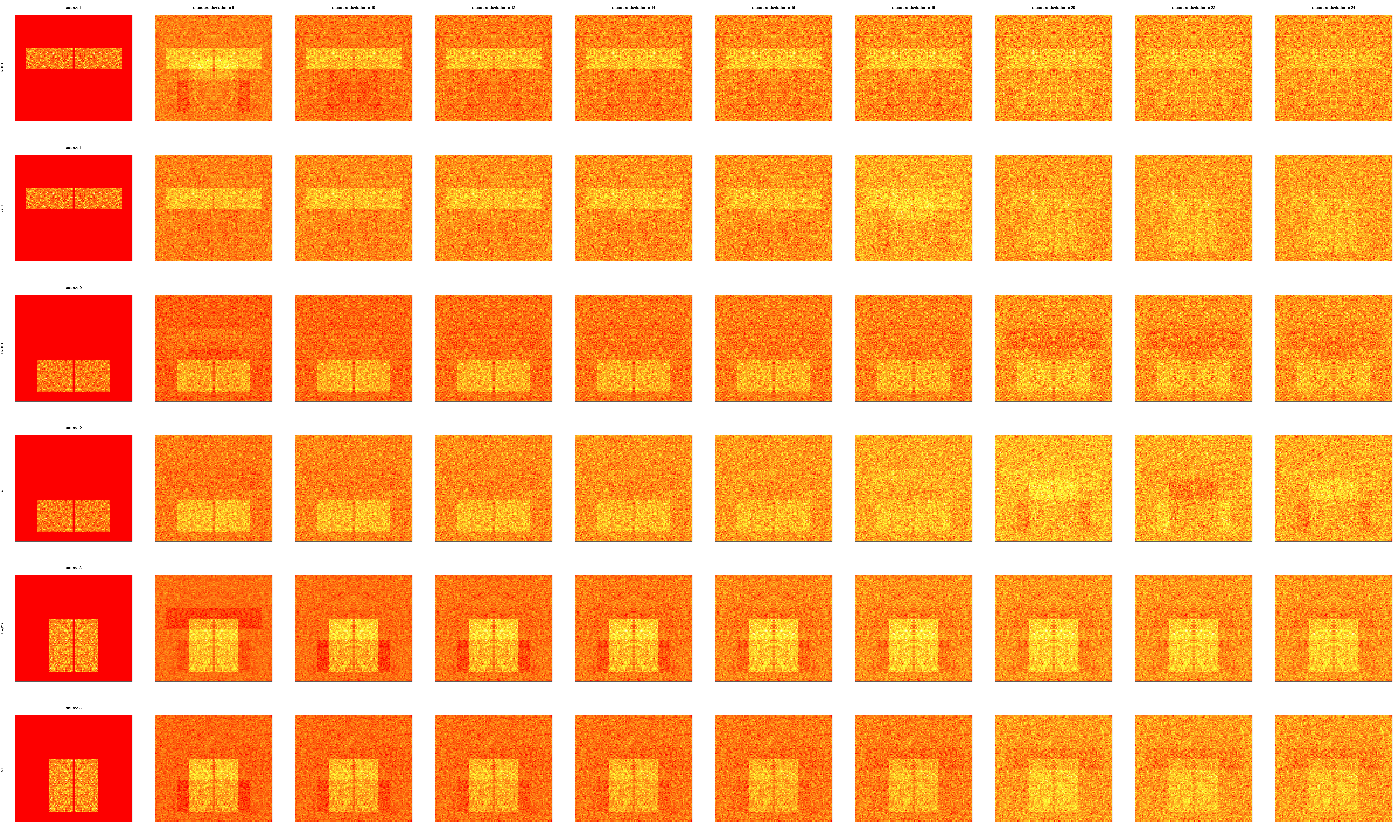
Figure 4 compares the ICs estimated by H-gICA and the ordinary gICA. As we can see, comparing with the ordinary gICA, H-gICA has a consistently better estimation of the ICs when noise exists.

Figure 4: The ICs estimated by H-gICA and gICA. The first column shows the true sources. The other columns, from left to right, show the estimated ICs when the noise increases. The $1^{st}$, $3^{rd}$, and $5^{th}$ rows are for H-gICA and the $2_{nd}$, $4^{th}$ and $6^{th}$ are for gICA.

4.2.2 Case II: Perfect Lateralization

True sources are now presumed to be only present in one hemisphere (perfect lateralization of the brain network), and without loss of generality, the left hemisphere is selected. Similar to Case I, a Gamma distribution was used to generate the value of the activated voxels and, again, 300 iterations were run. Figure 5 shows the heatplots of the three true sources in the first iteration.

Figure 5: True Sources in Non-homotopic Setting. All three true sources are only in one hemisphere. The values of the activated voxels are generated by Gamma distribution with different parameters.

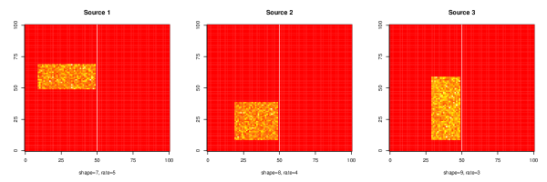
Gassian noise was added to the data generated by the three sources and the results are compared with ordinary gICA. Note that, since the independent components provided by H-gICA contain only one hemisphere by design. Thus, the sole applicable comparison is the true sources in the left hemisphere. Table 2 gives these results, and show that the mean error of H-gICA is less than that of gICA for Source 2 while larger than the mean error of gICA for Source 1 and Source 3. In summary, H-gICA is competitive with normal g-ICA when the sources are lateralized with the caveat that H-gICA does not provide lateralization information on which hemisphere the network resides in. We do note, however, that this information is contained in the temporal mixing matrix, just not in a form easily displayed as an image.

Table 2: Comparison of the H-gICA results versus ordinary gICA results when the true sources are only in one hemisphere. The table provides the mean and standard deviation of the voxel mean difference with the true sources for the 300 iterations.

	Source 1	Source 2	Source 3
H-gICA	0.508 ($\sim 0.002$)	0.494 ($\sim 0.001$)	0.431 ($\sim 0.002$)
gICA	0.502 ($\sim 0.003$)	0.533 ($\sim 0.002$)	0.312 ($\sim 0.003$)

4.2.3 Case III: Mixture of Lateralized and Homotopic Networks

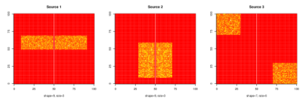
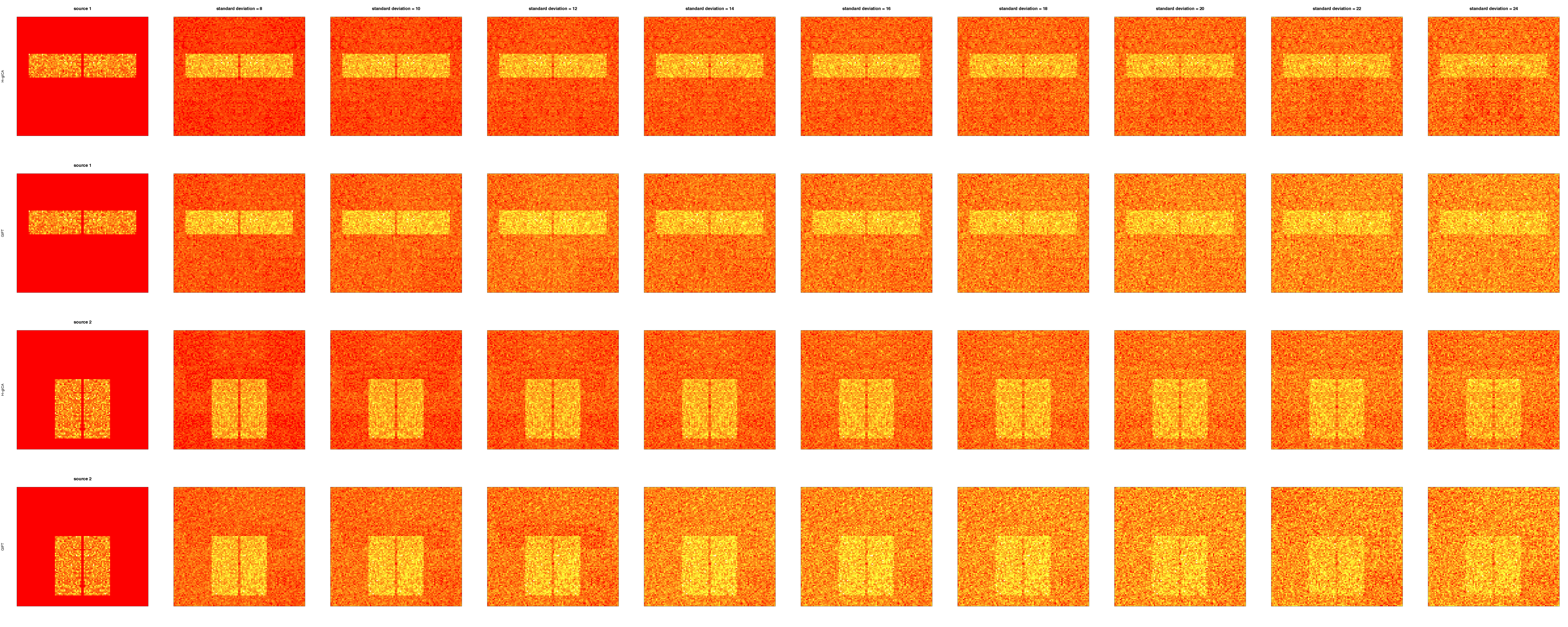
For this setting, a mixture of two different types of sources is introduced. As shown in Figure 6, the first two sources are homotopic while the third source covers different regions in the two hemispheres. The estimated ICs for the two homotopic sources are in Figure 7, which illustrates that the effectiveness of estimating the homotopic sources is not impacted by adding non-homotopic sources.

Figure 6: True Sources in Mixed Setting. The first two sources are homotopic while the third one varies in the two hemispheres.

Figure 7: The homotopic ICs estimated by H-gICA and ordinary gICA. The first column shows the true sources. The other columns, from left to right, contain the estimated ICs with increasing noise. The $1^{st}$ and $3^{rd}$ rows are results of H-gICA and the $2_{nd}$ and $4^{th}$ are of ordinary gICA.

4.3 Flag Example

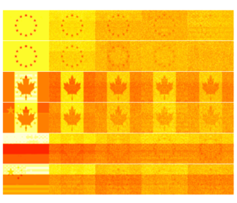
In this example, the actual sources will be the gray-scaled flags of the USA, Canada, the European Union, China and Russia. As shown in Figure 8, three of them are symmetric (Canada, the European Union and Russia) and two are not (USA and China). Similar as in Section 4.2, the data are generated by the ICA model with a fixed mixing matrix, Gaussian noise was then added. The results are shown in Figure 9, where the $1^{st}$, $3^{rd}$ and $5^{th}$ rows are the estimated symmetric sources extracted by H-gICA and the $2_{nd}$, $4^{th}$ and $6^{th}$ rows are the estimated symmetric sources extracted by ordinary gICA. As we can see, for all of the three symmetric sources, H-gICA provides clearer estimation as the noises increased. Moreover, leakage that is apparent in the g-ICA is not apparent in H-gICA.

Figure 8: Actual sources of the flag example. The original flags images were taken from Wikipedia.

Figure 9: The estimated homotopic sources of H-gICA and ordinary gICA. The five columns, from left to right, contain the estimated ICs with increasing noise. The $1^{st}$, $3^{rd}$ and $5^{th}$ rows shows the estimated sources extracted by H-gICA while the $2_{nd}$, $4^{th}$ and $6^{th}$ rows shows the estimated sources extracted by ordinary gICA.

5 Application to the ADHD-200 Dataset

Application of the H-gICA method is illustrated using the ADHD-200 dataset, one of the largest and freely available resting state fMRI datasets. The data combines 776 resting-state fMRI and anatomical scans aggregated across eight independent imaging sites, 491 of which were obtained from normally developing individuals and 285 from children and adolescents with ADHD (ages: 7-21 years old). We view this analysis as largely a proof of principle in applying the method and defer thorough investigations of ADHD for later work.

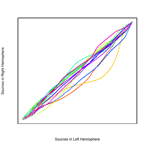
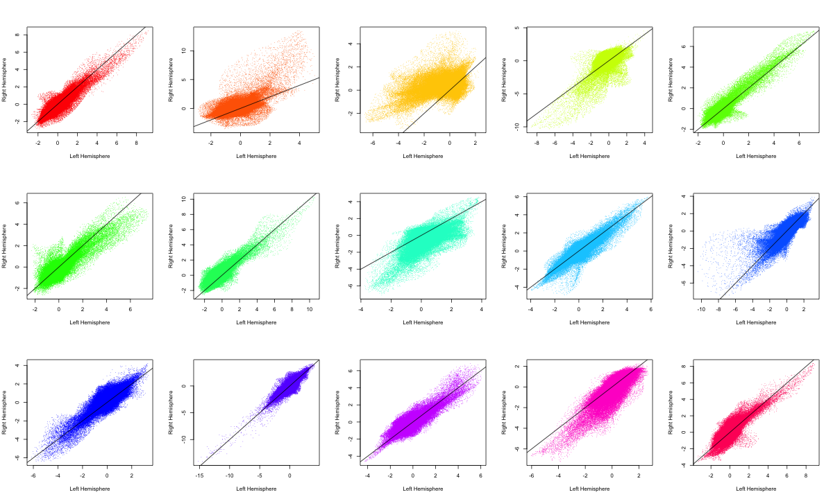
This particular analysis focused on 20 subjects picked from the ADHD-200 data set. Data were processed via the NITRC 1,000 Functional Connectome processing scripts (Mennes et al., 2012). In summary, images were slice-time corrected, deobliqued, skull stripped, smoothed and registered to a 3 mm3 MNI template. The data were then registered to ICBM 2009a nonlinear symmetric templates generated by the McConnell Brain Imaging Centre (Fonov et al., 2009b, 2011a). Each fMRI scan contains $99\times 117\times 95=1,100,385$ voxels measured at $176$ time points. Figure 10 and Figure 11 are the QQ plot and scatter plots of the estimated sources extracted by ordinary gICA in the left and right hemispheres. Most of the estimated sources are close to the $45^{o}$ line, which suggests that the marginal distributions of left and right hemispheres are similar. H-gICA can benefit from this apparent homotopy.

Figure 10: QQ plot of the 15 sources extracted by gICA.

Figure 11: The scatter plot of the 15 sources.

Our procedure is as follows. Each fMRI scan was separated into left and right hemispheres. Thus, each hemisphere contained $49\times 117\times 95=544,635$ voxels. Similar to standard group ICA (Calhoun et al., 2001b), a dimension reduction using PCA was applied to each hemisphere of each subject. 15 PCs are obtained for each hemisphere. A group data matrix was generated by concatenating the reduced data of both hemispheres of the 20 subjects in the temporal domain. Thus, the aggregated matrix has dimension $2NT\times V$, where $N=20$, $T=15$, and $V=544,635$. Our algorithm of homotopic group ICA is then applied on this matrix. Fifteen estimated independent components are postulated by H-gICA. As shown in Figure 12, out of the 15 components, several brain networks were found including: the visual network 12, the default mode network 12, the auditory network 12, and the motor network 12. Compared with the ICs obtained from ordinary gICA, shown in 12, 12, 12 and 12, H-gICA improves the estimation of all of these sources by yielding substantially more clearly delineated networks.

Figure 12: Comparison of ICs obtain from H-gICA (left column) and ordinary gICA (right column).

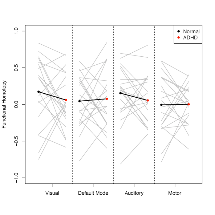
The approach of H-gICA also allows us to calculate the brain functional homotopy of each brain network. To compare the brain functional homotopy of ADHD and typical developed children, we choose 20 ADHD subjects and 20 subject-macthed controls. The subjects and controls were matched in gender and age. Via Equations (4) and (5), the estimated functional homotopy of four networks (visual, default mode, auditory and motor) are shown in Figure 13. As we can see, the functional homotopy of ADHD children tends to be lower in both visual networks and the auditory network. These represent meaningful leads on the exploration of homotopic network relationships and disease, though we leave a full exploration to later work.

Figure 13: Comparison of functional homotopy of ADHD and normal developed children. Each column represents a network (visual, default mode, auditory and motor). Each pair (subjects and controls) are connected via a grey line. The left end points of the grey lines measure the functional homotopy of the control and the right end points are for the ADHD subjects. The black lines represent the group level functional homotopy for the four networks.

6 Discussion

In this paper we present a new group ICA method called homotopic group ICA (H-gICA). Similar with ordinary group ICA methods, H-gICA can analyze data for multiple subjects and estimate common underlying IC’s across individuals. By concatenating the fMRI data of the two hemispheres, H-gICA effectively doubles the sample size. It improves the power of finding the underlying brain networks by rearranging the data structure and utilizing the known information of synchrony between bi-laterally symmetrically opposing inter-hemispheric regions. Both the simulation study and the application on ADHD 200 data show that H-gICA is preferable to ordinary gICA when the data are homotopic, increasingly so as noise increases. Moreover, H-gICA remains preferable to gICA at estimating homotopic sources, even in the presence of non-homotopic sources. Effectiveness was demonstrated by application on the ADHD-200 dataset. Several brain networks were found and clearly represented in smoother, more clearly delineated, contiguous volumes than ordinary gICA. The main networks found included visual networks, the default mode network, the auditory network, as well as others. Moreover H-gICA enables certain measurement of the functional homotopy of the underlying functional networks. This potentially offers the opportunity to analyze the relation of the brain functional homotopy between the left and right hemisphere of the brain with diseases.

Appendix

Proof of Theorem 3.1

Proof.

Since the true sources are truly homotopic and noise free, we have:

$$\mbox{\boldmath$X$}_{i,1}=\mbox{\boldmath$X$}_{i,2},$$

where $\mbox{\boldmath$X$}_{i,j}$, $j=1,2$, are the data of left and right hemispheres after dimension reduction by PCA. This is equivalent to

$$\mbox{\boldmath$X$}_{1}=\mbox{\boldmath$X$}_{2}.$$

Without loss of generality, we assume $\mbox{\boldmath$X$}_{j}$ ($j=1,2$) are demeaned i.e. the row means of $\mbox{\boldmath$X$}_{j}$ are all 0. Assume the singular value decomposition of the matrix $\mbox{\boldmath$X$}_{1}/\sqrt{V}$ is

$$\mbox{\boldmath$X$}_{1}/\sqrt{V}=\mbox{\boldmath$U$}\Sigma\mbox{\boldmath$V$}^{T},$$

where $U$ is of dimension $NQ\times(NQ-1)$ which consists of the left singular vectors of $\mbox{\boldmath$X$}_{1}$, $\Sigma$ is a diagonal matrix of dimension $(NQ-1)\times(NQ-1)$ with the singular values, and $V$ is of dimension $V\times(NQ-1)$ which consists of the right singular vectors. Both $U$ and $V$ are orthogonal. Note that, since $X$ is not full rank, only $NQ-1$ singular value are non-zero and thus only $NQ-1$ singular vectors are estimated. Then we have

$$\mbox{\boldmath$X$}/\sqrt{V} =[(\mbox{\boldmath$X$}_{1}/\sqrt{V})^{T},(\mbox{\boldmath$X$}_{2}/\sqrt{V})^{T}]^{T}$$

$$=[(\mbox{\boldmath$U$}\Sigma\mbox{\boldmath$V$}^{T})^{T},(\mbox{\boldmath$U$}\Sigma\mbox{\boldmath$V$}^{T})^{T}]^{T}$$

$$=[\mbox{\boldmath$U$}^{T},\mbox{\boldmath$U$}^{T}]^{T}\Sigma\mbox{\boldmath$V$}^{T}$$

and

$$\tilde{}\mbox{\boldmath$X$}/\sqrt{V} =[(\mbox{\boldmath$X$}_{1}/\sqrt{V}),(\mbox{\boldmath$X$}_{2}/\sqrt{V})]$$

$$=[(\mbox{\boldmath$U$}\Sigma\mbox{\boldmath$V$}^{T}),(\mbox{\boldmath$U$}\Sigma\mbox{\boldmath$V$}^{T})]$$

$$=\mbox{\boldmath$U$}\Sigma[\mbox{\boldmath$V$}^{T},\mbox{\boldmath$V$}^{T}].$$

Thus we can define

$$\mbox{\boldmath$K$}:=\frac{1}{2}\Sigma^{-1}[\mbox{\boldmath$U$},\mbox{\boldmath$U$}]\;\;\mbox{and}\;\;\tilde{\mbox{\boldmath$K$}}:=\Sigma^{-1}\mbox{\boldmath$U$}$$ (6)

to be the pre-whitening matrix that projects data onto the principal components:

$$\mbox{\boldmath$Z$}=\mbox{\boldmath$K$}\mbox{\boldmath$X$}\;\;\mbox{and}\;\;\tilde{\mbox{\boldmath$Z$}}=\tilde{\mbox{\boldmath$K$}}\tilde{\mbox{\boldmath$X$}},$$

where $\mbox{\boldmath$Z$}=\sqrt{V}\mbox{\boldmath$V$}^{T}$ and $\tilde{\mbox{\boldmath$Z$}}=[\sqrt{V}\mbox{\boldmath$V$}^{T},\sqrt{V}\mbox{\boldmath$V$}^{T}]$ are the whiten data for H-gICA and GIFT respectively. Clearly, if we assume the random variables $z$ and $\tilde{\mbox{\boldmath$z$}}$ are taking values from the columns of $Z$ and $\tilde{\mbox{\boldmath$Z$}}$, then we will have:

$$E[\mbox{\boldmath$z$}\mbox{\boldmath$z$}^{T}]=\mbox{\boldmath$I$}\;\;\mbox{and}\;\;E[\tilde{\mbox{\boldmath$z$}}\tilde{\mbox{\boldmath$z$}}^{T}]=\mbox{\boldmath$I$}.$$

Suppose we have the same initial value for the vectors $\mbox{\boldmath$w$}_{p}$ for all $p\in\{1,2,\cdots,Q\}$. No matter how the contrast function, $G$, is defined for each fixed $w$ we have:

$$E\{\mbox{\boldmath$z$}g(\mbox{\boldmath$w$}^{T}\mbox{\boldmath$z$})\} =\frac{1}{V}\sum\limits_{v=1}^{V}\mbox{\boldmath$Z$}(\cdot,v)g(\mbox{\boldmath$w$}^{T}\mbox{\boldmath$Z$}(\cdot,v))$$

$$=\sum\limits_{v=1}^{V}\mbox{\boldmath$V$}^{T}(\cdot,v)g(\mbox{\boldmath$w$}^{T}\mbox{\boldmath$V$}^{T}(\cdot,v))$$

$$=\frac{1}{2}\left(\sum\limits_{v=1}^{V}\mbox{\boldmath$V$}^{T}(\cdot,v)g(\mbox{\boldmath$w$}^{T}\mbox{\boldmath$V$}^{T}(\cdot,v))+\sum\limits_{v=1}^{V}\mbox{\boldmath$V$}^{T}(\cdot,v)g(\mbox{\boldmath$w$}^{T}\mbox{\boldmath$V$}^{T}(\cdot,v))\right)$$

$$=\frac{1}{2V}\sum\limits_{v=1}^{2V}\tilde{\mbox{\boldmath$Z$}}(\cdot,v)g(\mbox{\boldmath$w$}^{T}\tilde{\mbox{\boldmath$Z$}}(\cdot,v))$$

$$=E\{\tilde{\mbox{\boldmath$z$}}g(\mbox{\boldmath$w$}^{T}\tilde{\mbox{\boldmath$z$}})\}$$

where $g$ is defined as the derivative of the contrast function $G$. Similarly,

$$E\{g^{\prime}(\mbox{\boldmath$w$}^{T}\mbox{\boldmath$z$})\}\mbox{\boldmath$w$}=E\{g^{\prime}(\mbox{\boldmath$w$}^{T}\tilde{\mbox{\boldmath$z$}})\}\mbox{\boldmath$w$},$$

where $g$ is the derivative of $G$. So we have:

$$E\{\mbox{\boldmath$z$}g(\mbox{\boldmath$w$}^{T}\mbox{\boldmath$z$})\}-E\{g^{\prime}(\mbox{\boldmath$w$}^{T}\mbox{\boldmath$z$})\}\mbox{\boldmath$w$}=E\{\tilde{\mbox{\boldmath$z$}}g(\mbox{\boldmath$w$}^{T}\tilde{\mbox{\boldmath$z$}})\}-E\{g^{\prime}(\mbox{\boldmath$w$}^{T}\tilde{\mbox{\boldmath$z$}})\}\mbox{\boldmath$w$}$$

Thus, following the FastICA algorithm (Hyvärinen, 1999), it is easy to see that the estimates of $\mbox{\boldmath$w$}_{p}$, $p=1,2,\cdots,m$, will be same for these two approaches. By the definition of $K$ and $\tilde{\mbox{\boldmath$K$}}$ in (6), we will have:

$$\hat{\mbox{\boldmath$W$}} =[\mbox{\boldmath$w$}_{1},\mbox{\boldmath$w$}_{2},\cdots,\mbox{\boldmath$w$}_{m}]^{T}\mbox{\boldmath$K$}$$

$$=\frac{1}{2}[\mbox{\boldmath$w$}_{1},\mbox{\boldmath$w$}_{2},\cdots,\mbox{\boldmath$w$}_{m}]^{T}[\tilde{\mbox{\boldmath$K$}},\tilde{\mbox{\boldmath$K$}}]$$

$$=\frac{1}{2}[\hat{\tilde{\mbox{\boldmath$W$}}},\hat{\tilde{\mbox{\boldmath$W$}}}]$$

and

$$\hat{\mbox{\boldmath$S$}} =\hat{\mbox{\boldmath$W$}}\mbox{\boldmath$X$}=\frac{1}{2}[\hat{\tilde{\mbox{\boldmath$W$}}},\hat{\tilde{\mbox{\boldmath$W$}}}][\mbox{\boldmath$X$}_{1}^{T},\mbox{\boldmath$X$}_{2}^{T}]^{T}=\hat{\tilde{\mbox{\boldmath$W$}}}\mbox{\boldmath$X$}_{1}$$

$$\hat{\tilde{\mbox{\boldmath$S$}}} =\hat{\tilde{\mbox{\boldmath$W$}}}\tilde{\mbox{\boldmath$X$}}=\hat{\tilde{\mbox{\boldmath$W$}}}[\tilde{\mbox{\boldmath$X$}_{1}},\tilde{\mbox{\boldmath$X$}_{2}}]=\hat{\tilde{\mbox{\boldmath$W$}}}[\tilde{\mbox{\boldmath$X$}_{1}},\tilde{\mbox{\boldmath$X$}_{1}}]$$

Thus follows the result of Theorem 3.1. ∎

References

- Beckmann and Smith (2004) C.F. Beckmann and S.M. Smith. Probabilistic independent component analysis for functional magnetic resonance imaging. Medical Imaging, IEEE Transactions on, 23(2):137–152, 2004.
- Beckmann and Smith (2005) C.F. Beckmann and S.M. Smith. Tensorial extensions of independent component analysis for multisubject fmri analysis. Neuroimage, 25(1):294–311, 2005.
- Biswal et al. (1995) B. Biswal, F. Zerrin Yetkin, V.M. Haughton, and J.S. Hyde. Functional connectivity in the motor cortex of resting human brain using echo-planar mri. Magnetic resonance in medicine, 34(4):537–541, 1995.
- Calhoun et al. (2001a) VD Calhoun, T. Adali, VB McGinty, JJ Pekar, TD Watson, GD Pearlson, et al. fmri activation in a visual-perception task: network of areas detected using the general linear model and independent components analysis. NeuroImage, 14(5):1080–1088, 2001a.
- Calhoun et al. (2001b) VD Calhoun, T. Adali, GD Pearlson, and JJ Pekar. A method for making group inferences from functional mri data using independent component analysis. Human brain mapping, 14(3):140–151, 2001b.
- Comon (1994) P. Comon. Independent component analysis, a new concept? Signal processing, 36(3):287–314, 1994.
- Damoiseaux et al. (2008) JS Damoiseaux, CF Beckmann, E.J.S. Arigita, F. Barkhof, P. Scheltens, CJ Stam, SM Smith, and S. Rombouts. Reduced resting-state brain activity in the default network in normal aging. Cerebral Cortex, 18(8):1856–1864, 2008.
- Eloyan et al. (2012) Ani Eloyan, John Muschelli, Mary Beth Nebel, Han Liu, Fang Han, Tuo Zhao, Anita D Barber, Suresh Joel, James J Pekar, Stewart H Mostofsky, et al. Automated diagnoses of attention deficit hyperactive disorder using magnetic resonance imaging. Frontiers in Systems Neuroscience, 6:61, 2012.
- Eloyan et al. (2013) Ani Eloyan, Ciprian M. Crainiceanu, and Brian S. Caffo. Likelihood-based population independent component analysis. Biostatistics, 2013.
- Esposito et al. (2005) F. Esposito, T. Scarabino, A. Hyvarinen, J. Himberg, E. Formisano, S. Comani, G. Tedeschi, R. Goebel, E. Seifritz, F. Di Salle, et al. Independent component analysis of fmri group studies by self-organizing clustering. Neuroimage, 25(1):193–205, 2005.
- Fonov et al. (2011a) V. Fonov, A.C. Evans, K. Botteron, C.R. Almli, R.C. McKinstry, and D.L. Collins. Unbiased average age-appropriate atlases for pediatric studies. NeuroImage, 54(1):313, 2011a.
- Fonov et al. (2011b) Vladimir Fonov, Alan C Evans, Kelly Botteron, C Robert Almli, Robert C McKinstry, and D Louis Collins. Unbiased average age-appropriate atlases for pediatric studies. NeuroImage, 54(1):313, 2011b.
- Fonov et al. (2009a) VS Fonov, AC Evans, RC McKinstry, CR Almli, and DL Collins. Unbiased nonlinear average age-appropriate brain templates from birth to adulthood. NeuroImage, 47:S102, 2009a.
- Fonov et al. (2009b) VS Fonov, AC Evans, RC McKinstry, CR Almli, and DL Collins. Unbiased nonlinear average age-appropriate brain templates from birth to adulthood. Neuroimage, 47:S102, 2009b.
- Gao et al. (2009) Wei Gao, Hongtu Zhu, Kelly S Giovanello, J Keith Smith, Dinggang Shen, John H Gilmore, and Weili Lin. Evidence on the emergence of the brain’s default network from 2-week-old to 2-year-old healthy pediatric subjects. Proceedings of the National Academy of Sciences, 106(16):6790–6795, 2009.
- Gao et al. (2012) Wei Gao, John H Gilmore, Dinggang Shen, Jeffery Keith Smith, Hongtu Zhu, and Weili Lin. The synchronization within and interaction between the default and dorsal attention networks in early infancy. Cerebral Cortex, 2012.
- Garrity et al. (2007) A. Garrity, G. Pearlson, K. McKiernan, D. Lloyd, K. Kiehl, and V. Calhoun. Aberrant default mode functional connectivity in schizophrenia. American Journal of Psychiatry, 164(3):450–457, 2007.
- Guo and Pagnoni (2008) Y. Guo and G. Pagnoni. A unified framework for group independent component analysis for multi-subject fmri data. NeuroImage, 42(3):1078–1093, 2008.
- Gusnard et al. (2001) D.A. Gusnard, M.E. Raichle, ME Raichle, et al. Searching for a baseline: functional imaging and the resting human brain. Nature Reviews Neuroscience, 2(10):685–694, 2001.
- Hyvärinen (1999) A. Hyvärinen. Fast and robust fixed-point algorithms for independent component analysis. Neural Networks, IEEE Transactions on, 10(3):626–634, 1999.
- Joel et al. (2011) S.E. Joel, B.S. Caffo, P. van Zijl, and J.J. Pekar. On the relationship between seed-based and ica-based measures of functional connectivity. Magnetic Resonance in Medicine, 66(3):644–657, 2011.
- McKeown et al. (1997) M.J. McKeown, S. Makeig, G.G. Brown, T.P. Jung, S.S. Kindermann, A.J. Bell, and T.J. Sejnowski. Analysis of fmri data by blind separation into independent spatial components. Technical report, DTIC Document, 1997.
- Mennes et al. (2012) M. Mennes, B. Biswal, F.X. Castellanos, and M.P. Milham. Making data sharing work: The fcp/indi experience. NeuroImage, 2012.
- Milham (2012) M.P. Milham. Open neuroscience solutions for the connectome-wide association era. Neuron, 73(2):214–218, 2012.
- Oja et al. (2001) E. Oja, A. Hyvarinen, and J. Karhunen. Independent component analysis, 2001.
- Pillai et al. (2002) S.U. Pillai et al. Probability, Random Variables, and Stochastic Processes. Tata McGraw-Hill Education, 2002.
- Rombouts et al. (2005) S.A.R.B. Rombouts, F. Barkhof, R. Goekoop, C.J. Stam, and P. Scheltens. Altered resting state networks in mild cognitive impairment and mild alzheimer’s disease: an fmri study. Human brain mapping, 26(4):231–239, 2005.
- Sambataro et al. (2010) F. Sambataro, V.P. Murty, J.H. Callicott, H.Y. Tan, S. Das, D.R. Weinberger, and V.S. Mattay. Age-related alterations in default mode network: impact on working memory performance. Neurobiology of aging, 31(5):839, 2010.
- Sorg et al. (2007) C. Sorg, V. Riedl, M. Mühlau, V.D. Calhoun, T. Eichele, L. Läer, A. Drzezga, H. Förstl, A. Kurz, C. Zimmer, et al. Selective changes of resting-state networks in individuals at risk for alzheimer’s disease. Proceedings of the National Academy of Sciences, 104(47):18760–18765, 2007.
- Toro et al. (2008) R. Toro, P.T. Fox, and T. Paus. Functional coactivation map of the human brain. Cerebral cortex, 18(11):2553–2559, 2008.
- Zuo et al. (2010) X.N. Zuo, C. Kelly, A. Di Martino, M. Mennes, D.S. Margulies, S. Bangaru, R. Grzadzinski, A.C. Evans, Y.F. Zang, F.X. Castellanos, et al. Growing together and growing apart: regional and sex differences in the lifespan developmental trajectories of functional homotopy. The Journal of Neuroscience, 30(45):15034–15043, 2010.