Exact Methods for Multistage Estimation of a Binomial Proportion

ZhengjiaChenZhengjiaChen{\mathrm{Zhengjia}\;\mathrm{Chen}\;} and Xinjia Chen Dr. Zhengjia Chen is working with Department of Biostatistics and Bioinformatics, Emory University, Atlanta, GA 30322; Email: zchen38@emory.edu. Dr. Xinjia Chen is working with Department of Electrical Engineering, Southern University at Baton Rouge, LA 70813; Email: xinjiachen@engr.subr.edu.
(February 2013)
Abstract

We first review existing sequential methods for estimating a binomial proportion. Afterward, we propose a new family of group sequential sampling schemes for estimating a binomial proportion with prescribed margin of error and confidence level. In particular, we establish the uniform controllability of coverage probability and the asymptotic optimality for such a family of sampling schemes. Our theoretical results establish the possibility that the parameters of this family of sampling schemes can be determined so that the prescribed level of confidence is guaranteed with little waste of samples. Analytic bounds for the cumulative distribution functions and expectations of sample numbers are derived. Moreover, we discuss the inherent connection of various sampling schemes. Numerical issues are addressed for improving the accuracy and efficiency of computation. Computational experiments are conducted for comparing sampling schemes. Illustrative examples are given for applications in clinical trials.

1 Introduction

Estimating a binomial proportion is a problem of ubiquitous significance in many areas of engineering and sciences. For economical reasons and other concerns, it is important to use as fewer as possible samples to guarantee the required reliability of estimation. To achieve this goal, sequential sampling schemes can be very useful. In a sequential sampling scheme, the total number of observations is not fixed in advance. The sampling process is continued stage by stage until a pre-specified stopping rule is satisfied. The stopping rule is evaluated with accumulated observations. In many applications, for administrative feasibility, the sampling experiment is performed in a group fashion. Similar to group sequential tests [5, Section 8], [27], an estimation method based on taking samples by groups and evaluating them sequentially is referred to as a group sequential estimation method. It should be noted that group sequential estimation methods are general enough to include fixed-sample-size and fully sequential procedures as special cases. Particularly, a fixed-sample-size method can be viewed as a group sequential procedure of only one stage. If the increment between the sample sizes of consecutive stages is equal to 111, then the group sequential method is actually a fully sequential method.

It is a common contention that statistical inference, as a unique science to quantify the uncertainties of inferential statements, should avoid errors in the quantification of uncertainties, while minimizing the sampling cost. That is, a statistical inferential method is expected to be exact and efficient. The conventional notion of exactness is that no approximation is involved, except the roundoff error due to finite word length of computers. Existing sequential methods for estimating a binomial proportion are dominantly of asymptotic nature (see, e.g., [6, 24, 25, 28, 33] and the references therein). Undoubtedly, asymptotic techniques provide approximate solutions and important insights for the relevant problems. However, any asymptotic method inevitably introduces unknown error in the resultant approximate solution due to the necessary use of a finite number of samples. In the direction of non-asymptotic sequential estimation, the primary goal is to ensure that the true coverage probability is above the pre-specified confidence level for any value of the associated parameter, while the required sample size is as low as possible. In this direction, Mendo and Hernando [31] developed an inverse binomial sampling scheme for estimating a binomial proportion with relative precision. Tanaka [34] developed a rigorous method for constructing fixed-width sequential confidence intervals for a binomial proportion. Although no approximation is involved, Tanaka’s method is very conservative due to the bounding techniques employed in the derivation of sequential confidence intervals. Franzén [21] studied the construction of fixed-width sequential confidence intervals for a binomial proportion. However, no effective method for defining stopping rules is proposed in [21]. In his later paper [22], Franzén proposed to construct fixed-width confidence intervals based on sequential probability ratio tests (SPRTs) invented by Wald [35]. His method can generate fixed-sample-size confidence intervals based on SPRTs. Unfortunately, he made a fundamental flaw by mistaking that if the width of the fixed-sample-size confidence interval decreases to be smaller than the pre-specified length as the number of samples is increasing, then the fixed-sample-size confidence interval at the termination of sampling process is the desired fixed-width sequential confidence interval guaranteeing the prescribed confidence level. More recently, Jesse Frey published a paper [23] in The American Statistician (TAS) on the classical problem of sequentially estimating a binomial proportion with prescribed margin of error and confidence level. Before Frey submitted his original manuscript to TAS in July 2009, a general framework of multistage parameter estimation had been established by Chen [7, 9, 11, 13, 14], which provides exact methods for estimating parameters of common distributions with various error criterion. This framework is also proposed in [15]. The approach of Frey [23] is similar to that of Chen [7, 9, 11, 13, 14] for the specific problem of estimating a binomial proportion with prescribed margin of error and confidence level.

In this paper, our primary interests are in the exact sequential methods for the estimation of a binomial proportion with prescribed margin of error and confidence level. We first introduce the exact approach established in [7, 9, 11, 13, 14]. In particular, we introduce the inclusion principle proposed in [14] and its applications to the construction of concrete stopping rules. We investigate the connection among various stopping rules. Afterward, we propose a new family of stopping rules which are extremely simple and accommodate some existing stopping rules as special cases. We provide rigorous justification for the feasibility and asymptotic optimality of such stopping rules. We prove that the prescribed confidence level can be guaranteed uniformly for all values of a binomial proportion by choosing appropriate parametric values for the stopping rule. We show that as the margin of error tends to zero, the sample size tends to the attainable minimum as if the binomial proportion were exactly known. We derive analytic bounds for distributions and expectations of sample numbers. In addition, we address some critical computational issues and propose methods to improve the accuracy and efficiency of numerical calculation. We conduct extensive numerical experiment to study the performance of various stopping rules. We determine parametric values for the proposed stopping rules to achieve unprecedentedly efficiency while guaranteeing prescribed confidence levels. We attempt to make our proposed method as user-friendly as possible so that it can be immediately applicable even for layer persons.

The remainder of the paper is organized as follows. In Section 2, we introduce the exact approach proposed in [7, 9, 11, 13, 14]. In Section 3, we discuss the general principle of constructing stopping rules. In Section 4, we propose a new family of sampling schemes and investigate their feasibility, optimality and analytic bounds of the distribution and expectation of sample numbers. In Section 5, we compare various computational methods. In particular, we illustrate why the natural method of evaluating coverage probability based on gridding parameter space is neither rigorous nor efficient. In Section 6, we present numerical results for various sampling schemes. In Section 7, we illustrate the applications of our group sequential method in clinical trials. Section 8 is the conclusion. The proofs of theorems are given in appendices. Throughout this paper, we shall use the following notations. The empty set is denoted by \emptyset. The set of positive integers is denoted by \mathbb{N}. The ceiling function is denoted by .\lceil.\rceil. The notation Pr{Eθ}Prconditional𝐸𝜃\Pr\{E\mid\theta\} denotes the probability of the event E𝐸E associated with parameter θ𝜃\theta. The expectation of a random variable is denoted by 𝔼[.]\mathbb{E}[.]. The standard normal distribution is denoted by Φ(.)\Phi(.). For α(0,1)𝛼01\alpha\in(0,1), the notation 𝒵αsubscript𝒵𝛼\mathcal{Z}_{\alpha} denotes the critical value such that Φ(𝒵α)=1αΦsubscript𝒵𝛼1𝛼\Phi(\mathcal{Z}_{\alpha})=1-\alpha. For n𝑛n\in\mathbb{N}, in the case that X1,,Xnsubscript𝑋1subscript𝑋𝑛X_{1},\cdots,X_{n} are i.i.d. samples of X𝑋X, we denote the sample mean i=1nXinsuperscriptsubscript𝑖1𝑛subscript𝑋𝑖𝑛\frac{\sum_{i=1}^{n}X_{i}}{n} by X¯nsubscript¯𝑋𝑛\overline{X}_{n}, which is also called the relative frequency when X𝑋X is a Bernoulli random variable. The other notations will be made clear as we proceed.

2 How Can It Be Exact?

In many areas of scientific investigation, the outcome of an experiment is of dichotomy nature and can be modeled as a Bernoulli random variable X𝑋X, defined in probability space (Ω,Pr,)ΩPr(\Omega,\Pr,\mathscr{F}), such that

Pr{X=1}=1Pr{X=0}=p(0,1),Pr𝑋11Pr𝑋0𝑝01\Pr\{X=1\}=1-\Pr\{X=0\}=p\in(0,1),

where p𝑝p is referred to as a binomial proportion. In general, there is no analytical method for evaluating the binomial proportion p𝑝p. A frequently-used approach is to estimate p𝑝p based on i.i.d. samples X1,X2,subscript𝑋1subscript𝑋2X_{1},X_{2},\cdots of X𝑋X. To reduce the sampling cost, it is appropriate to estimate p𝑝p by a multistage sampling procedure. More formally, let ε(0,1)𝜀01\varepsilon\in(0,1) and 1δ1𝛿1-\delta, with δ(0,1)𝛿01\delta\in(0,1), be the pre-specified margin of error and confidence level respectively. The objective is to construct a sequential estimator 𝒑^^𝒑\widehat{\boldsymbol{p}} for p𝑝p based on a multistage sampling scheme such that

Pr{|𝒑^p|<εp}1δPr^𝒑𝑝bra𝜀𝑝1𝛿\Pr\{|\widehat{\boldsymbol{p}}-p|<\varepsilon\mid p\}\geq 1-\delta (1)

for any p(0,1)𝑝01p\in(0,1). Throughout this paper, the probability Pr{|𝒑^p|<εp}Pr^𝒑𝑝bra𝜀𝑝\Pr\{|\widehat{\boldsymbol{p}}-p|<\varepsilon\mid p\} is referred to as the coverage probability. Accordingly, the probability Pr{|𝒑^p|εp}Pr^𝒑𝑝conditional𝜀𝑝\Pr\{|\widehat{\boldsymbol{p}}-p|\geq\varepsilon\mid p\} is referred to as the complementary coverage probability. Clearly, a complete construction of a multistage estimation scheme needs to determine the number of stages, the sample sizes for all stages, the stopping rule, and the estimator for p𝑝p. Throughout this paper, we let s𝑠s denote the number of stages and let nsubscript𝑛n_{\ell} denote the number of samples at the \ell-th stages. That is, the sampling process consists of s𝑠s stages with sample sizes n1<n2<<nssubscript𝑛1subscript𝑛2subscript𝑛𝑠n_{1}<n_{2}<\cdots<n_{s}. For =1,2,,s12𝑠\ell=1,2,\cdots,s, define K=i=1nXisubscript𝐾superscriptsubscript𝑖1subscript𝑛subscript𝑋𝑖K_{\ell}=\sum_{i=1}^{n_{\ell}}X_{i} and 𝒑^=Knsubscript^𝒑subscript𝐾subscript𝑛\widehat{\boldsymbol{p}}_{\ell}=\frac{K_{\ell}}{n_{\ell}}. The stopping rule is to be defined in terms of 𝒑^,=1,,sformulae-sequencesubscript^𝒑1𝑠\widehat{\boldsymbol{p}}_{\ell},\;\ell=1,\cdots,s. Of course, the index of stage at the termination of the sampling process, denoted by 𝒍𝒍\boldsymbol{l}, is a random number. Accordingly, the number of samples at the termination of the experiment, denoted by 𝐧𝐧\mathbf{n}, is a random number which equals n𝒍subscript𝑛𝒍n_{\boldsymbol{l}}. Since for each \ell, 𝒑^subscript^𝒑\widehat{\boldsymbol{p}}_{\ell} is a maximum-likelihood and minimum-variance unbiased estimator of p𝑝p, the sequential estimator for p𝑝p is taken as

𝒑^=𝒑^𝒍=i=1n𝒍Xin𝒍=i=1𝐧Xi𝐧.^𝒑subscript^𝒑𝒍superscriptsubscript𝑖1subscript𝑛𝒍subscript𝑋𝑖subscript𝑛𝒍superscriptsubscript𝑖1𝐧subscript𝑋𝑖𝐧\widehat{\boldsymbol{p}}=\widehat{\boldsymbol{p}}_{\boldsymbol{l}}=\frac{\sum_{i=1}^{n_{\boldsymbol{l}}}X_{i}}{n_{\boldsymbol{l}}}=\frac{\sum_{i=1}^{\mathbf{n}}X_{i}}{\mathbf{n}}. (2)

In the above discussion, we have outlined the general characteristics of a multistage sampling scheme for estimating a binomial proportion. It remains to determine the number of stages, the sample sizes for all stages, and the stopping rule so that the resultant estimator 𝒑^^𝒑\widehat{\boldsymbol{p}} satisfies (1) for any p(0,1)𝑝01p\in(0,1).

Actually, the problem of sequential estimation of a binomial proportion has been treated by Chen [7, 9, 11, 13, 14] in a general framework of multistage parameter estimation. The techniques of [7, 9, 11, 13, 14] are sufficient to offer exact solutions for a wide range of sequential estimation problems, including the estimation of a binomial proportion as a special case. The central idea of the approach in [7, 9, 11, 13, 14] is the control of coverage probability by a single parameter ζ𝜁\zeta, referred to as the coverage tuning parameter, and the adaptive rigorous checking of coverage guarantee by virtue of bounds of coverage probabilities. It is recognized in [7, 9, 11, 13, 14] that, due to the discontinuity of the coverage probability on parameter space, the conventional method of evaluating the coverage probability for a finite number of parameter values is neither rigorous not computationally efficient for checking the coverage probability guarantee.

As mentioned in the introduction, Frey published an article [23] in TAS on the sequential estimation of a binomial proportion with prescribed margin of error and confidence level. For clarity of presentation, the comparison of the works of Chen and Frey is given in Section 5.4. In the remainder of this section, we shall only introduce the idea and techniques of [7, 9, 11, 13, 14], which had been precedentially developed by Chen before Frey submitted his original manuscript to TAS in July 2009. We will introduce the approach of [7, 9, 11, 13, 14] with a focus on the special problem of estimating a binomial proportion with prescribed margin of error and confidence level.

2.1 Four Components Suffice

The exact methods of [7, 9, 11, 13, 14] for multistage parameter estimation have four main components as follows:

(I) Stopping rules parameterized by the coverage tuning parameter ζ>0𝜁0\zeta>0 such that the associated coverage probabilities can be made arbitrarily close to 111 by choosing ζ>0𝜁0\zeta>0 to be a sufficiently small number.

(II) Recursively computable lower and upper bounds for the complementary coverage probability for a given ζ𝜁\zeta and an interval of parameter values.

(III) Adapted Branch and Bound Algorithm.

(IV) Bisection coverage tuning.

Without looking at the technical details, one can see that these four components are sufficient for constructing a sequential estimator so that the prescribed confidence level is guaranteed. The reason is as follows: As lower and upper bounds for the complementary coverage probability are available, the global optimization technique, Branch and Bound (B&B) Algorithm [29], can be used to compute exactly the maximum of complementary coverage probability on the whole parameter space. Thus, it is possible to check rigorously whether the coverage probability associated with a given ζ𝜁\zeta is no less than the pre-specified confidence level. Since the coverage probability can be controlled by ζ𝜁\zeta, it is possible to determine ζ𝜁\zeta as large as possible to guarantee the desired confidence level by a bisection search. This process is referred to as bisection coverage tuning in [7, 9, 11, 13, 14]. Since a critical subroutine needed for bisection coverage tuning is to check whether the coverage probability is no less than the pre-specified confidence level, it is not necessary to compute exactly the maximum of the complementary coverage probability. Therefore, Chen revised the standard B&B algorithm to reduce the computational complexity and called the improved algorithm as the Adapted B&B Algorithm. The idea is to adaptively partition the parameter space as many subintervals. If for all subintervals, the upper bounds of the complementary coverage probability are no greater than δ𝛿\delta, then declare that the coverage probability is guaranteed. If there exists a subinterval for which the lower bound of the complementary coverage probability is greater than δ𝛿\delta, then declare that the coverage probability is not guaranteed. Continue partitioning the parameter space if no decision can be made. The four components are illustrated in the sequel under the headings of stopping rules, interval bounding, adapted branch and bound, and bisection coverage tuning.

2.2 Stopping Rules

The first component for the exact sequential estimation of a binomial proportion is the stopping rule for constructing a sequential estimator such that the coverage probability can be controlled by the coverage tuning parameter ζ𝜁\zeta. For convenience of describing some concrete stopping rules, define

(z,θ)={zlnθz+(1z)ln1θ1zforz(0,1)andθ(0,1),ln(1θ)forz=0andθ(0,1),lnθforz=1andθ(0,1),forz[0,1]andθ(0,1)𝑧𝜃cases𝑧𝜃𝑧1𝑧1𝜃1𝑧for𝑧01and𝜃011𝜃for𝑧0and𝜃01𝜃for𝑧1and𝜃01for𝑧01and𝜃01\mathscr{M}(z,\theta)=\begin{cases}z\ln\frac{\theta}{z}+(1-z)\ln\frac{1-\theta}{1-z}&\text{for}\;z\in(0,1)\;\text{and}\;\theta\in(0,1),\\ \ln(1-\theta)&\text{for}\;z=0\;\text{and}\;\theta\in(0,1),\\ \ln\theta&\text{for}\;z=1\;\text{and}\;\theta\in(0,1),\\ -\infty&\text{for}\;z\in[0,1]\;\text{and}\;\theta\notin(0,1)\end{cases}

and

S(k,l,n,p)={i=kl(ni)pi(1p)niforp(0,1),0forp(0,1)𝑆𝑘𝑙𝑛𝑝casessuperscriptsubscript𝑖𝑘𝑙binomial𝑛𝑖superscript𝑝𝑖superscript1𝑝𝑛𝑖for𝑝010for𝑝01S(k,l,n,p)=\begin{cases}\sum_{i=k}^{l}\binom{n}{i}p^{i}(1-p)^{n-i}&\text{for}\;p\in(0,1),\\ 0&\text{for}\;p\notin(0,1)\end{cases}

where k𝑘k and l𝑙l are integers such that 0kln0𝑘𝑙𝑛0\leq k\leq l\leq n. Assume that 0<ζδ<10𝜁𝛿10<\zeta\delta<1. For the purpose of controlling the coverage probability Pr{|𝒑^p|<εp}Pr^𝒑𝑝bra𝜀𝑝\Pr\{|\widehat{\boldsymbol{p}}-p|<\varepsilon\mid p\} by the coverage tuning parameter, Chen has proposed four stopping rules as follows:

Stopping Rule A: Continue sampling until (12|12𝒑^|,12|12𝒑^|+ε)ln(ζδ)n1212subscript^𝒑1212subscript^𝒑𝜀𝜁𝛿subscript𝑛\mathscr{M}(\frac{1}{2}-|\frac{1}{2}-\widehat{\boldsymbol{p}}_{\ell}|,\frac{1}{2}-|\frac{1}{2}-\widehat{\boldsymbol{p}}_{\ell}|+\varepsilon)\leq\frac{\ln(\zeta\delta)}{n_{\ell}} for some {1,,s}1𝑠\ell\in\{1,\cdots,s\}.

Stopping Rule B: Continue sampling until (|𝒑^12|23ε)214+ε2n2ln(ζδ)superscriptsubscript^𝒑1223𝜀214superscript𝜀2subscript𝑛2𝜁𝛿(|\widehat{\boldsymbol{p}}_{\ell}-\frac{1}{2}|-\frac{2}{3}\varepsilon)^{2}\geq\frac{1}{4}+\frac{\varepsilon^{2}n_{\ell}}{2\ln(\zeta\delta)} for some {1,,s}1𝑠\ell\in\{1,\cdots,s\}.

Stopping Rule C: Continue sampling until S(K,n,n,𝒑^ε)ζδ𝑆subscript𝐾subscript𝑛subscript𝑛subscript^𝒑𝜀𝜁𝛿S(K_{\ell},n_{\ell},n_{\ell},\widehat{\boldsymbol{p}}_{\ell}-\varepsilon)\leq\zeta\delta and S(0,K,n,𝒑^+ε)ζδ𝑆0subscript𝐾subscript𝑛subscript^𝒑𝜀𝜁𝛿S(0,K_{\ell},n_{\ell},\widehat{\boldsymbol{p}}_{\ell}+\varepsilon)\leq\zeta\delta for some {1,,s}1𝑠\ell\in\{1,\cdots,s\}.

Stopping Rule D: Continue sampling until n𝒑^(1𝒑^)2ε2ln1ζδsubscript𝑛subscript^𝒑1subscript^𝒑2superscript𝜀21𝜁𝛿n_{\ell}\geq\widehat{\boldsymbol{p}}_{\ell}(1-\widehat{\boldsymbol{p}}_{\ell})\frac{2}{\varepsilon^{2}}\ln\frac{1}{\zeta\delta} for some {1,,s}1𝑠\ell\in\{1,\cdots,s\}.

Stopping Rule A was first proposed in [7, Theorem 7] and restated in [9, Theorem 16]. Stopping Rule B was first proposed in [11, Theorem 1] and represented as the third stopping rule in [10, Section 4.1.1]. Stopping Rule C originated from [13, Theorem 1] and was restated as the first stopping rule in [10, Section 4.1.1]. Stopping Rule D was described in the remarks following Theorem 7 of [8]. All these stopping rules can be derived from the general principles proposed in [14, Section 3] and [15, Section 2.4].

Given that a stopping rule can be expressed in terms of 𝒑^subscript^𝒑\widehat{\boldsymbol{p}}_{\ell} and nsubscript𝑛n_{\ell} for =1,,s1𝑠\ell=1,\cdots,s, it is possible to find a bivariate function 𝒟(.,.)\mathscr{D}(.,.) on {(z,n):z[0,1],n}conditional-set𝑧𝑛formulae-sequence𝑧01𝑛\{(z,n):z\in[0,1],\;n\in\mathbb{N}\}, taking values from {0,1}01\{0,1\}, such that the stopping rule can be stated as: Continue sampling until 𝒟(𝒑^,n)=1𝒟subscript^𝒑subscript𝑛1\mathscr{D}(\widehat{\boldsymbol{p}}_{\ell},n_{\ell})=1 for some {1,,s}1𝑠\ell\in\{1,\cdots,s\}. It can be checked that such representation applies to Stopping Rules A, B, C, and D. For example, Stopping Rule B can be expressed in this way by virtue of function 𝒟(.,.)\mathscr{D}(.,.) such that

𝒟(z,n)={1if (|z12|23ε)214+ε2n2ln(ζδ),0otherwise𝒟𝑧𝑛cases1if (|z12|23ε)214+ε2n2ln(ζδ)0otherwise\mathscr{D}(z,n)=\begin{cases}1&\text{if {\small$(|z-\frac{1}{2}|-\frac{2}{3}\varepsilon)^{2}\geq\frac{1}{4}+\frac{\varepsilon^{2}n}{2\ln(\zeta\delta)}$}},\\ 0&\text{otherwise}\end{cases}

The motivation of introducing function 𝒟(.,.)\mathscr{D}(.,.) is to parameterize the stopping rule in terms of design parameters. The function 𝒟(.,.)\mathscr{D}(.,.) determines the form of the stopping rule and consequently, the sample sizes for all stages can be chosen as functions of design parameters. Specifically, let

Nmin=min{n:𝒟(kn,n)=1for some nonnegative integer k not exceeding n},subscript𝑁min:𝑛𝒟𝑘𝑛𝑛1for some nonnegative integer k not exceeding n\displaystyle N_{\mathrm{min}}=\min\left\{n\in\mathbb{N}:\mathscr{D}\left(\frac{k}{n},n\right)=1\;\text{for some nonnegative integer $k$ not exceeding $n$}\right\},\qquad\qquad (3)
Nmax=min{n:𝒟(kn,n)=1for all nonnegative integer k not exceeding n}.subscript𝑁max:𝑛𝒟𝑘𝑛𝑛1for all nonnegative integer k not exceeding n\displaystyle N_{\mathrm{max}}=\min\left\{n\in\mathbb{N}:\mathscr{D}\left(\frac{k}{n},n\right)=1\;\text{for all nonnegative integer $k$ not exceeding $n$}\right\}. (4)

To avoid unnecessary checking of the stopping criterion and thus reduce administrative cost, there should be a possibility that the sampling process is terminated at the first stage. Hence, the minimum sample size n1subscript𝑛1n_{1} should be chosen to ensure that {𝐧=n1}𝐧subscript𝑛1\{\mathbf{n}=n_{1}\}\neq\emptyset. This implies that the sample size n1subscript𝑛1n_{1} for the first stage can be taken as Nminsubscript𝑁minN_{\mathrm{min}}. On the other hand, since the sampling process must be terminated at or before the s𝑠s-th stage, the maximum sample size nssubscript𝑛𝑠n_{s} should be chosen to guarantee that {𝐧>ns}=𝐧subscript𝑛𝑠\{\mathbf{n}>n_{s}\}=\emptyset. This implies that the sample size nssubscript𝑛𝑠n_{s} for the last stage can be taken as Nmaxsubscript𝑁maxN_{\mathrm{max}}. If the number of stages s𝑠s is given, then the sample sizes for stages in between 111 and s𝑠s can be chosen as s2𝑠2s-2 integers between Nminsubscript𝑁minN_{\mathrm{min}} and Nmaxsubscript𝑁maxN_{\mathrm{max}}. Specially, if the group sizes are expected to be approximately equal, then the sample sizes can be taken as

n=Nmin+1s1(NmaxNmin),=1,,s.formulae-sequencesubscript𝑛subscript𝑁min1𝑠1subscript𝑁maxsubscript𝑁min1𝑠n_{\ell}=\left\lceil N_{\mathrm{min}}+\frac{\ell-1}{s-1}(N_{\mathrm{max}}-N_{\mathrm{min}})\right\rceil,\qquad\ell=1,\cdots,s. (5)

Since the stopping rule is associated with the coverage tuning parameter ζ𝜁\zeta, it follows that the number of stages s𝑠s and the sample sizes n1,n2,,nssubscript𝑛1subscript𝑛2subscript𝑛𝑠n_{1},n_{2},\cdots,n_{s} can be expressed as functions of ζ𝜁\zeta. In this sense, it can be said that the stopping rule is parameterized by the coverage tuning parameter ζ𝜁\zeta. The above method of parameterizing stopping rules has been used in [7, 9, 11, 13] and proposed in [10, Section 2.1, page 9].

2.3 Interval Bounding

The second component for the exact sequential estimation of a binomial proportion is the method of bounding the complementary coverage probability Pr{|𝒑^p|εp}Pr^𝒑𝑝conditional𝜀𝑝\Pr\{|\widehat{\boldsymbol{p}}-p|\geq\varepsilon\mid p\} for p𝑝p in an interval [a,b]𝑎𝑏[a,b] contained by interval (0,1)01(0,1). Applying Theorem 8 of [9] to the special case of a Bernoulli distribution immediately yields

Pr{𝒑^aεb}+Pr{𝒑^b+εa}Pr{|𝒑^p|εp}Pr{𝒑^bεa}+Pr{𝒑^a+εb}Pr^𝒑𝑎conditional𝜀𝑏Pr^𝒑𝑏conditional𝜀𝑎Pr^𝒑𝑝conditional𝜀𝑝Pr^𝒑𝑏conditional𝜀𝑎Pr^𝒑𝑎conditional𝜀𝑏\Pr\{\widehat{\boldsymbol{p}}\leq a-\varepsilon\mid b\}+\Pr\{\widehat{\boldsymbol{p}}\geq b+\varepsilon\mid a\}\leq\Pr\{|\widehat{\boldsymbol{p}}-p|\geq\varepsilon\mid p\}\leq\Pr\{\widehat{\boldsymbol{p}}\leq b-\varepsilon\mid a\}+\Pr\{\widehat{\boldsymbol{p}}\geq a+\varepsilon\mid b\}\qquad (6)

for all p[a,b](0,1)𝑝𝑎𝑏01p\in[a,b]\subseteq(0,1). The bounds of (6) can be shown as follows: Note that Pr{𝒑^aεp}+Pr{𝒑^b+εp}Pr{|𝒑^p|εp}=Pr{𝒑^pεp}+Pr{𝒑^p+εp}Pr{𝒑^bεp}+Pr{𝒑^a+εp}Pr^𝒑𝑎conditional𝜀𝑝Pr^𝒑𝑏conditional𝜀𝑝Pr^𝒑𝑝conditional𝜀𝑝Pr^𝒑𝑝conditional𝜀𝑝Pr^𝒑𝑝conditional𝜀𝑝Pr^𝒑𝑏conditional𝜀𝑝Pr^𝒑𝑎conditional𝜀𝑝\Pr\{\widehat{\boldsymbol{p}}\leq a-\varepsilon\mid p\}+\Pr\{\widehat{\boldsymbol{p}}\geq b+\varepsilon\mid p\}\leq\Pr\{|\widehat{\boldsymbol{p}}-p|\geq\varepsilon\mid p\}=\Pr\{\widehat{\boldsymbol{p}}\leq p-\varepsilon\mid p\}+\Pr\{\widehat{\boldsymbol{p}}\geq p+\varepsilon\mid p\}\leq\Pr\{\widehat{\boldsymbol{p}}\leq b-\varepsilon\mid p\}+\Pr\{\widehat{\boldsymbol{p}}\geq a+\varepsilon\mid p\} for p[a,b](0,1)𝑝𝑎𝑏01p\in[a,b]\subseteq(0,1). As a consequence of the monotonicity of Pr{𝒑^ϑp}Pr^𝒑conditionalitalic-ϑ𝑝\Pr\{\widehat{\boldsymbol{p}}\geq\vartheta\mid p\} and Pr{𝒑^ϑp}Pr^𝒑conditionalitalic-ϑ𝑝\Pr\{\widehat{\boldsymbol{p}}\leq\vartheta\mid p\} with respect to p𝑝p, where ϑitalic-ϑ\vartheta is a real number independent of p𝑝p, the lower and upper bounds of Pr{|𝒑^p|εp}Pr^𝒑𝑝conditional𝜀𝑝\Pr\{|\widehat{\boldsymbol{p}}-p|\geq\varepsilon\mid p\} for p[a,b](0,1)𝑝𝑎𝑏01p\in[a,b]\subseteq(0,1) can be given as Pr{𝒑^aεb}+Pr{𝒑^b+εa}Pr^𝒑𝑎conditional𝜀𝑏Pr^𝒑𝑏conditional𝜀𝑎\Pr\{\widehat{\boldsymbol{p}}\leq a-\varepsilon\mid b\}+\Pr\{\widehat{\boldsymbol{p}}\geq b+\varepsilon\mid a\} and Pr{𝒑^bεa}+Pr{𝒑^a+εb}Pr^𝒑𝑏conditional𝜀𝑎Pr^𝒑𝑎conditional𝜀𝑏\Pr\{\widehat{\boldsymbol{p}}\leq b-\varepsilon\mid a\}+\Pr\{\widehat{\boldsymbol{p}}\geq a+\varepsilon\mid b\} respectively.

In page 15, equation (1) of [9], Chen proposed to apply the recursive method of Schultz [32, Section 2] to compute the lower and upper bounds of Pr{|𝒑^p|εp}Pr^𝒑𝑝conditional𝜀𝑝\Pr\{|\widehat{\boldsymbol{p}}-p|\geq\varepsilon\mid p\} given by (6). It should be pointed out that such lower and upper bounds of Pr{|𝒑^p|εp}Pr^𝒑𝑝conditional𝜀𝑝\Pr\{|\widehat{\boldsymbol{p}}-p|\geq\varepsilon\mid p\} can also be computed by the recursive path-counting method of Franzén [21, page 49].

2.4 Adapted Branch and Bound

The third component for the exact sequential estimation of a binomial proportion is the Adapted B&B Algorithm, which was proposed in [9, Section 2.8], for quick determination of whether the coverage probability is no less than 1δ1𝛿1-\delta for any value of the associated parameter. Such a task of checking the coverage probability is also referred to as checking the coverage probability guarantee. Given that lower and upper bounds of the complementary coverage probability on an interval of parameter values can be obtained by the interval bounding techniques, this task can be accomplished by applying the B&B Algorithm [29] to compute exactly the maximum of the complementary coverage probability on the parameter space. However, in our applications, it suffices to determine whether the maximum of the complementary coverage probability Pr{|𝒑^p|εp}Pr^𝒑𝑝conditional𝜀𝑝\Pr\{|\widehat{\boldsymbol{p}}-p|\geq\varepsilon\mid p\} with respect to p(0,1)𝑝01p\in(0,1) is greater than the confidence parameter δ𝛿\delta. For fast checking whether the maximal complementary coverage probability exceeds δ𝛿\delta, Chen proposed to reduce the computational complexity by revising the standard B&B Algorithm as the Adapted B&B Algorithm in [9, Section 2.8]. To describe this algorithm, let initsubscriptinit\mathcal{I}_{\mathrm{init}} denote the parameter space (0,1)01(0,1). For an interval initsubscriptinit\mathcal{I}\subseteq\mathcal{I}_{\mathrm{init}}, let maxΨ()Ψ\max\Psi(\mathcal{I}) denote the maximum of the complementary coverage probability Pr{|𝒑^p|εp}Pr^𝒑𝑝conditional𝜀𝑝\Pr\{|\widehat{\boldsymbol{p}}-p|\geq\varepsilon\mid p\} with respect to p𝑝p\in\mathcal{I}. Let Ψlb()subscriptΨlb\Psi_{\mathrm{lb}}(\mathcal{I}) and Ψub()subscriptΨub\Psi_{\mathrm{ub}}(\mathcal{I}) be respectively the lower and upper bounds of Ψ()Ψ\Psi(\mathcal{I}), which can be obtained by the interval bounding techniques introduced in Section 2.3. Let η>0𝜂0\eta>0 be a pre-specified tolerance, which is much smaller than δ𝛿\delta. The Adapted B&B Algorithm of [9] is represented with a slight modification as follows.


Letk0,l0Ψlb(init)andu0Ψub(init)formulae-sequenceLet𝑘0subscript𝑙0subscriptΨlbsubscriptinitandsubscript𝑢0subscriptΨubsubscriptinit\nabla\;\text{Let}\;k\leftarrow 0,\;l_{0}\leftarrow\Psi_{\mathrm{lb}}(\mathcal{I}_{\mathrm{init}})\;\text{and}\;u_{0}\leftarrow\Psi_{\mathrm{ub}}(\mathcal{I}_{\mathrm{init}}).
Let𝒮0{init}if u0>δ. Otherwise, let 𝒮0 be emptyLetsubscript𝒮0subscriptinitif u0>δ. Otherwise, let 𝒮0 be empty\nabla\;\text{Let}\;\mathscr{S}_{0}\leftarrow\{\mathcal{I}_{\mathrm{init}}\}\;\text{if $u_{0}>\delta$. Otherwise, let $\mathscr{S}_{0}$ be empty}.
While 𝒮k is nonempty, lk<δ and uk is greater than max{lk+η,δ}, do the following:While 𝒮k is nonempty, lk<δ and uk is greater than max{lk+η,δ}, do the following:\nabla\;\text{While $\mathscr{S}_{k}$ is nonempty, $l_{k}<\delta$ and $u_{k}$ is greater than $\max\{l_{k}+\eta,\;\delta\}$, do the following:}
Split each interval in 𝒮kas two new intervals of equal length.Split each interval in 𝒮kas two new intervals of equal length\indent\indent\diamond\;\text{Split each interval in $\mathscr{S}_{k}$}\;\text{as two new intervals of equal length}.
    Let Sksubscript𝑆𝑘S_{k} denote the set of all new intervals obtained from this splitting procedure.
Eliminate any interval  from Sk such that Ψub()δEliminate any interval  from Sk such that Ψub()δ\indent\indent\diamond\;\text{Eliminate any interval $\mathcal{I}$ from $S_{k}$ such that $\Psi_{\mathrm{ub}}(\mathcal{I})\leq\delta$}.
Let𝒮k+1be the set Sk processed by the above elimination procedureLetsubscript𝒮𝑘1be the set Sk processed by the above elimination procedure\indent\indent\diamond\;\text{Let}\;\mathscr{S}_{k+1}\;\text{be the set $S_{k}$ processed by the above elimination procedure}.
Letlk+1max𝒮k+1Ψlb()anduk+1max𝒮k+1Ψub()Letsubscript𝑙𝑘1subscriptsubscript𝒮𝑘1subscriptΨlbandsubscript𝑢𝑘1subscriptsubscript𝒮𝑘1subscriptΨub\indent\indent\diamond\;\text{Let}\;l_{k+1}\leftarrow\max_{\mathcal{I}\in\mathscr{S}_{k+1}}\Psi_{\mathrm{lb}}(\mathcal{I})\;\text{and}\;u_{k+1}\leftarrow\max_{\mathcal{I}\in\mathscr{S}_{k+1}}\Psi_{\mathrm{ub}}(\mathcal{I}). Letkk+1Let𝑘𝑘1\text{Let}\;k\leftarrow k+1.
If 𝒮k is empty and lk<δ, then declare maxΨ(init)δIf 𝒮k is empty and lk<δ, then declare maxΨ(init)δ\nabla\;\text{If $\mathscr{S}_{k}$ is empty and $l_{k}<\delta$, then declare $\max\Psi(\mathcal{I}_{\mathrm{init}})\leq\delta$}.
    Otherwise, declare maxΨ(init)>δΨsubscriptinit𝛿\max\Psi(\mathcal{I}_{\mathrm{init}})>\delta.

It should be noted that for a sampling scheme of symmetrical stopping boundary, the initial interval initsubscriptinit\mathcal{I}_{\mathrm{init}} may be taken as (0,12)012(0,\frac{1}{2}) for the sake of efficiency. In Section 5.1, we will illustrate why the Adapted B&B Algorithm is superior than the direct evaluation based on gridding parameter space. As will be seen in Section 5.2, the objective of the Adapted B&B Algorithm can also be accomplished by the Adaptive Maximum Checking Algorithm due to Chen [10, Section 3.3 ] and rediscovered by Frey in the second revision of his manuscript submitted to TAS in April 2010 [23, Appendix]. An explanation is given in Section 5.3 for the advantage of working with the complementary coverage probability.

2.5 Bisection Coverage Tuning

The fourth component for the exact sequential estimation of a binomial proportion is Bisection Coverage Tuning. Based on the adaptive rigorous checking of coverage probability, Chen proposed in [7, Section 2.7] and [9, Section 2.6] to apply a bisection search method to determine maximal ζ𝜁\zeta such that the coverage probability is no less than 1δ1𝛿1-\delta for any value of the associated parameter. Moreover, Chen has developed asymptotic results in [9, page 21, Theorem 18] for determining the initial interval of ζ𝜁\zeta needed for the bisection search. Specifically, if the complementary coverage probability Pr{|𝒑^p|εp}Pr^𝒑𝑝conditional𝜀𝑝\Pr\{|\widehat{\boldsymbol{p}}-p|\geq\varepsilon\mid p\} associated with ζ=ζ0𝜁subscript𝜁0\zeta=\zeta_{0} tends to δ𝛿\delta as ε0𝜀0\varepsilon\to 0, then the initial interval of ζ𝜁\zeta can be taken as [ζ02i,ζ02i+1]subscript𝜁0superscript2𝑖subscript𝜁0superscript2𝑖1[\zeta_{0}2^{i},\;\zeta_{0}2^{i+1}], where i𝑖i is the largest integer such that the complementary coverage probability associated with ζ=ζ02i𝜁subscript𝜁0superscript2𝑖\zeta=\zeta_{0}2^{i} is no greater than δ𝛿\delta for all p(0,1)𝑝01p\in(0,1). By virtue of a bisection search, it is possible to obtain ζ[ζ02i,ζ02i+1]superscript𝜁subscript𝜁0superscript2𝑖subscript𝜁0superscript2𝑖1\zeta^{*}\in[\zeta_{0}2^{i},\;\zeta_{0}2^{i+1}] such that the complementary coverage probability associated with ζ=ζ𝜁superscript𝜁\zeta=\zeta^{*} is guaranteed to be no greater than δ𝛿\delta for all p(0,1)𝑝01p\in(0,1).

3 Principle of Constructing Stopping Rules

In this section, we shall illustrate the inherent connection between various stopping rules. It will be demonstrated that a lot of stopping rules can be derived by virtue of the inclusion principle proposed by Chen [14, Section 3].

3.1 Inclusion Principle

The problem of estimating a binomial proportion can be considered as a special case of parameter estimation for a random variable X𝑋X parameterized by θΘ𝜃Θ\theta\in\Theta, where the objective is to construct a sequential estimator 𝜽^^𝜽\widehat{\boldsymbol{\theta}} for θ𝜃\theta such that Pr{|𝜽^θ|<εθ}1δPr^𝜽𝜃bra𝜀𝜃1𝛿\Pr\{|\widehat{\boldsymbol{\theta}}-\theta|<\varepsilon\mid\theta\}\geq 1-\delta for any θΘ𝜃Θ\theta\in\Theta. Assume that the sampling process consists of s𝑠s stages with sample sizes n1<n2<<nssubscript𝑛1subscript𝑛2subscript𝑛𝑠n_{1}<n_{2}<\cdots<n_{s}. For =1,,s1𝑠\ell=1,\cdots,s, define an estimator 𝜽^subscript^𝜽\widehat{\boldsymbol{\theta}}_{\ell} for θ𝜃\theta in terms of samples X1,,Xnsubscript𝑋1subscript𝑋subscript𝑛X_{1},\cdots,X_{n_{\ell}} of X𝑋X. Let [L,U],=1,2,,sformulae-sequencesubscript𝐿subscript𝑈12𝑠[L_{\ell},U_{\ell}],\;\ell=1,2,\cdots,s be a sequence of confidence intervals such that for any \ell, [L,U]subscript𝐿subscript𝑈[L_{\ell},U_{\ell}] is defined in terms of X1,,Xnsubscript𝑋1subscript𝑋subscript𝑛X_{1},\cdots,X_{n_{\ell}} and that the coverage probability Pr{LθUθ}Prsubscript𝐿𝜃conditionalsubscript𝑈𝜃\Pr\{L_{\ell}\leq\theta\leq U_{\ell}\mid\theta\} can be made arbitrarily close to 111 by choosing ζ>0𝜁0\zeta>0 to be a sufficiently small number. In Theorem 2 of [14], Chen proposed the following general stopping rule:

Continue sampling until Uε𝜽^L+ε for some {1,,s}.Continue sampling until Uε𝜽^L+ε for some {1,,s}\text{Continue sampling until {\small$U_{\ell}-\varepsilon\leq\widehat{\boldsymbol{\theta}}_{\ell}\leq L_{\ell}+\varepsilon$} for some $\ell\in\{1,\cdots,s\}$}. (7)

At the termination of the sampling process, a sequential estimator for θ𝜃\theta is taken as 𝜽^=𝜽^𝒍^𝜽subscript^𝜽𝒍\widehat{\boldsymbol{\theta}}=\widehat{\boldsymbol{\theta}}_{\boldsymbol{l}}, where 𝒍𝒍\boldsymbol{l} is the index of stage at the termination of sampling process.

Clearly, the general stopping rule (7) can be restated as follows:

Continue sampling until the confidence interval [L,U]subscript𝐿subscript𝑈[L_{\ell},U_{\ell}] is included by interval [𝜽^ε,𝜽^+ε]subscript^𝜽𝜀subscript^𝜽𝜀[\widehat{\boldsymbol{\theta}}_{\ell}-\varepsilon,\;\widehat{\boldsymbol{\theta}}_{\ell}+\varepsilon] for some {1,,s}1𝑠\ell\in\{1,\cdots,s\}.

The sequence of confidence intervals are parameterized by ζ𝜁\zeta for purpose of controlling the coverage probability Pr{|𝜽^θ|<εθ}Pr^𝜽𝜃bra𝜀𝜃\Pr\{|\widehat{\boldsymbol{\theta}}-\theta|<\varepsilon\mid\theta\}. Due to the inclusion relationship [L,U][𝜽^ε,𝜽^+ε]subscript𝐿subscript𝑈subscript^𝜽𝜀subscript^𝜽𝜀[L_{\ell},U_{\ell}]\subseteq[\widehat{\boldsymbol{\theta}}_{\ell}-\varepsilon,\;\widehat{\boldsymbol{\theta}}_{\ell}+\varepsilon], such a general methodology of using a sequence of confidence intervals to construct a stopping rule for controlling the coverage probability is referred to as the inclusion principle. It is asserted by Theorem 2 of [14] that

Pr{|𝜽^θ|<εθ}1sζδθΘformulae-sequencePr^𝜽𝜃bra𝜀𝜃1𝑠𝜁𝛿for-all𝜃Θ\Pr\{|\widehat{\boldsymbol{\theta}}-\theta|<\varepsilon\mid\theta\}\geq 1-s\zeta\delta\quad\forall\theta\in\Theta (8)

provided that Pr{L<θ<Uθ}1ζδPrsubscript𝐿𝜃brasubscript𝑈𝜃1𝜁𝛿\Pr\{L_{\ell}<\theta<U_{\ell}\mid\theta\}\geq 1-\zeta\delta for =1,,s1𝑠\ell=1,\cdots,s and θΘ𝜃Θ\theta\in\Theta. This demonstrates that if the number of stages s𝑠s is bounded with respective to ζ𝜁\zeta, then the coverage probability Pr{|𝜽^θ|<εθ}Pr^𝜽𝜃bra𝜀𝜃\Pr\{|\widehat{\boldsymbol{\theta}}-\theta|<\varepsilon\mid\theta\} associated with the stopping rule derived from the inclusion principle can be controlled by ζ𝜁\zeta. Actually, before explicitly proposing the inclusion principle in [14], Chen had extensively applied the inclusion principle in [7, 9, 11, 13] to construct stopping rules for estimating parameters of various distributions such as binomial, Poisson, geometric, hypergeometric, normal distributions, etc. A more general version of the inclusion principle is proposed in [15, Section 2.4]. For simplicity of the stopping rule, Chen had made effort to eliminate the computation of confidence limits.

In the context of estimating a binomial proportion p𝑝p, the inclusion principle immediately leads to the following general stopping rule:

Continue sampling until 𝒑^εLU𝒑^+εsubscript^𝒑𝜀subscript𝐿subscript𝑈subscript^𝒑𝜀\widehat{\boldsymbol{p}}_{\ell}-\varepsilon\leq L_{\ell}\leq U_{\ell}\leq\widehat{\boldsymbol{p}}_{\ell}+\varepsilon for some {1,,s}1𝑠\ell\in\{1,\cdots,s\}. (9)

Consequently, the sequential estimator for p𝑝p is taken as 𝒑^^𝒑\widehat{\boldsymbol{p}} according to (2). It should be pointed out that the stopping rule (9) had been rediscovered by Frey in Section 2, the 1st paragraph of [23]. The four stopping rules considered in his paper follow immediately from applying various confidence intervals to the general stopping rule (9).

In the sequel, we will illustrate how to apply (9) to the derivation of Stopping Rules A, B, C, D introduced in Section 2.2 and other specific stopping rules.

3.2 Stopping Rule from Wald Intervals

By virtue of Wald’s method of interval estimation for a binomial proportion p𝑝p, a sequence of confidence intervals [L,U],=1,,sformulae-sequencesubscript𝐿subscript𝑈1𝑠[L_{\ell},U_{\ell}],\;\ell=1,\cdots,s for p𝑝p can be constructed such that

L=𝒑^𝒵ζδ𝒑^(1𝒑^)n,U=𝒑^+𝒵ζδ𝒑^(1𝒑^)n,=1,,sformulae-sequencesubscript𝐿subscript^𝒑subscript𝒵𝜁𝛿subscript^𝒑1subscript^𝒑subscript𝑛formulae-sequencesubscript𝑈subscript^𝒑subscript𝒵𝜁𝛿subscript^𝒑1subscript^𝒑subscript𝑛1𝑠L_{\ell}=\widehat{\boldsymbol{p}}_{\ell}-\mathcal{Z}_{\zeta\delta}\sqrt{\frac{\widehat{\boldsymbol{p}}_{\ell}(1-\widehat{\boldsymbol{p}}_{\ell})}{n_{\ell}}},\qquad U_{\ell}=\widehat{\boldsymbol{p}}_{\ell}+\mathcal{Z}_{\zeta\delta}\sqrt{\frac{\widehat{\boldsymbol{p}}_{\ell}(1-\widehat{\boldsymbol{p}}_{\ell})}{n_{\ell}}},\qquad\ell=1,\cdots,s

and that Pr{LpUp}12ζδPrsubscript𝐿𝑝conditionalsubscript𝑈𝑝12𝜁𝛿\Pr\{L_{\ell}\leq p\leq U_{\ell}\mid p\}\approx 1-2\zeta\delta for =1,,s1𝑠\ell=1,\cdots,s and p(0,1)𝑝01p\in(0,1). Note that, for =1,,s1𝑠\ell=1,\cdots,s, the event {𝒑^εLU𝒑^+ε}subscript^𝒑𝜀subscript𝐿subscript𝑈subscript^𝒑𝜀\{\widehat{\boldsymbol{p}}_{\ell}-\varepsilon\leq L_{\ell}\leq U_{\ell}\leq\widehat{\boldsymbol{p}}_{\ell}+\varepsilon\} is the same as the event {(𝒑^12)214n(ε𝒵ζδ)2}superscriptsubscript^𝒑12214subscript𝑛superscript𝜀subscript𝒵𝜁𝛿2\left\{\left(\widehat{\boldsymbol{p}}_{\ell}-\frac{1}{2}\right)^{2}\geq\frac{1}{4}-n_{\ell}\left(\frac{\varepsilon}{\mathcal{Z}_{\zeta\delta}}\right)^{2}\right\}. So, applying this sequence of confidence intervals to (9) results in the stopping rule “continue sampling until (𝒑^12)214n(ε𝒵ζδ)2superscriptsubscript^𝒑12214subscript𝑛superscript𝜀subscript𝒵𝜁𝛿2\left(\widehat{\boldsymbol{p}}_{\ell}-\frac{1}{2}\right)^{2}\geq\frac{1}{4}-n_{\ell}\left(\frac{\varepsilon}{\mathcal{Z}_{\zeta\delta}}\right)^{2} for some {1,,s}1𝑠\ell\in\{1,\cdots,s\}”. Since for any ζ(0,1δ)𝜁01𝛿\zeta\in(0,\frac{1}{\delta}), there exists a unique number ζ(0,1δ)superscript𝜁01𝛿\zeta^{\prime}\in(0,\frac{1}{\delta}) such that 𝒵ζδ=2ln1ζδsubscript𝒵𝜁𝛿21superscript𝜁𝛿\mathcal{Z}_{\zeta\delta}=\sqrt{2\ln\frac{1}{\zeta^{\prime}\delta}}, this stopping rule is equivalent to “Continue sampling until (𝒑^12)214+ε2n2ln(ζδ)superscriptsubscript^𝒑12214superscript𝜀2subscript𝑛2𝜁𝛿\left(\widehat{\boldsymbol{p}}_{\ell}-\frac{1}{2}\right)^{2}\geq\frac{1}{4}+\frac{\varepsilon^{2}n_{\ell}}{2\ln(\zeta\delta)} for some {1,,s}1𝑠\ell\in\{1,\cdots,s\}.” This stopping rule is actually the same as Stopping Rule D, since {(𝒑^12)214+ε2n2ln(ζδ)}={n𝒑^(1𝒑^)2ε2ln1ζδ}superscriptsubscript^𝒑12214superscript𝜀2subscript𝑛2𝜁𝛿subscript𝑛subscript^𝒑1subscript^𝒑2superscript𝜀21𝜁𝛿\left\{\left(\widehat{\boldsymbol{p}}_{\ell}-\frac{1}{2}\right)^{2}\geq\frac{1}{4}+\frac{\varepsilon^{2}n_{\ell}}{2\ln(\zeta\delta)}\right\}=\left\{n_{\ell}\geq\widehat{\boldsymbol{p}}_{\ell}(1-\widehat{\boldsymbol{p}}_{\ell})\frac{2}{\varepsilon^{2}}\ln\frac{1}{\zeta\delta}\right\} for {1,,s}1𝑠\ell\in\{1,\cdots,s\}.

3.3 Stopping Rule from Revised Wald Intervals

Define 𝒑~=n𝒑^+an+2asubscript~𝒑subscript𝑛subscript^𝒑𝑎subscript𝑛2𝑎\widetilde{\boldsymbol{p}}_{\ell}=\frac{n_{\ell}\;\widehat{\boldsymbol{p}}_{\ell}+a}{n_{\ell}+2a} for =1,,s1𝑠\ell=1,\cdots,s, where a𝑎a is a positive number. Inspired by Wald’s method of interval estimation for p𝑝p, a sequence of confidence intervals [L,U],=1,,sformulae-sequencesubscript𝐿subscript𝑈1𝑠[L_{\ell},U_{\ell}],\;\ell=1,\cdots,s can be constructed such that

L=𝒑^𝒵ζδ𝒑~(1𝒑~)n,U=𝒑^+𝒵ζδ𝒑~(1𝒑~)nformulae-sequencesubscript𝐿subscript^𝒑subscript𝒵𝜁𝛿subscript~𝒑1subscript~𝒑subscript𝑛subscript𝑈subscript^𝒑subscript𝒵𝜁𝛿subscript~𝒑1subscript~𝒑subscript𝑛L_{\ell}=\widehat{\boldsymbol{p}}_{\ell}-\mathcal{Z}_{\zeta\delta}\sqrt{\frac{\widetilde{\boldsymbol{p}}_{\ell}(1-\widetilde{\boldsymbol{p}}_{\ell})}{n_{\ell}}},\qquad U_{\ell}=\widehat{\boldsymbol{p}}_{\ell}+\mathcal{Z}_{\zeta\delta}\sqrt{\frac{\widetilde{\boldsymbol{p}}_{\ell}(1-\widetilde{\boldsymbol{p}}_{\ell})}{n_{\ell}}}

and that Pr{LpUp}12ζδPrsubscript𝐿𝑝conditionalsubscript𝑈𝑝12𝜁𝛿\Pr\{L_{\ell}\leq p\leq U_{\ell}\mid p\}\approx 1-2\zeta\delta for =1,,s1𝑠\ell=1,\cdots,s and p(0,1)𝑝01p\in(0,1). This sequence of confidence intervals was applied by Frey [23] to the general stopping rule (9). As a matter of fact, such idea of revising Wald interval [X¯n𝒵ζδX¯n(1X¯n)n,X¯n+𝒵ζδX¯n(1X¯n)n]subscript¯𝑋𝑛subscript𝒵𝜁𝛿subscript¯𝑋𝑛1subscript¯𝑋𝑛𝑛subscript¯𝑋𝑛subscript𝒵𝜁𝛿subscript¯𝑋𝑛1subscript¯𝑋𝑛𝑛\left[\;\overline{X}_{n}-\mathcal{Z}_{\zeta\delta}\sqrt{\frac{\overline{X}_{n}(1-\overline{X}_{n})}{n}},\;\;\overline{X}_{n}+\mathcal{Z}_{\zeta\delta}\sqrt{\frac{\overline{X}_{n}(1-\overline{X}_{n})}{n}}\;\right] by replacing the relative frequency X¯n=i=1nXinsubscript¯𝑋𝑛superscriptsubscript𝑖1𝑛subscript𝑋𝑖𝑛\overline{X}_{n}=\frac{\sum_{i=1}^{n}X_{i}}{n} involved in the confidence limits with p~a=nX¯n+an+2asubscript~𝑝𝑎𝑛subscript¯𝑋𝑛𝑎𝑛2𝑎\widetilde{p}_{a}=\frac{n\overline{X}_{n}+a}{n+2a} had been proposed by H. Chen [4, Section 4].

As can be seen from Section 2, page 243, of Frey [23], applying (9) with the sequence of revised Wald intervals yields the stopping rule “Continue sampling until (𝒑~12)214+ε2n2ln(ζδ)superscriptsubscript~𝒑12214superscript𝜀2subscript𝑛2𝜁𝛿\left(\widetilde{\boldsymbol{p}}_{\ell}-\frac{1}{2}\right)^{2}\geq\frac{1}{4}+\frac{\varepsilon^{2}n_{\ell}}{2\ln(\zeta\delta)} for some {1,,s}1𝑠\ell\in\{1,\cdots,s\}.” Clearly, replacing 𝒑^subscript^𝒑\widehat{\boldsymbol{p}}_{\ell} in Stopping Rule D with 𝒑~=a+n𝒑^n+2asubscript~𝒑𝑎subscript𝑛subscript^𝒑subscript𝑛2𝑎\widetilde{\boldsymbol{p}}_{\ell}=\frac{a+n_{\ell}\widehat{\boldsymbol{p}}_{\ell}}{n_{\ell}+2a} also leads to this stopping rule.

3.4 Stopping Rule from Wilson’s Confidence Intervals

Making use of the interval estimation method of Wilson [36], one can obtain a sequence of confidence intervals [L,U],=1,,sformulae-sequencesubscript𝐿subscript𝑈1𝑠[L_{\ell},U_{\ell}],\;\ell=1,\cdots,s for p𝑝p such that

L=max{0,𝒑^+𝒵ζδ22n𝒵ζδ𝒑^(1𝒑^)n+(𝒵ζδ2n)21+𝒵ζδ2n},U=min{1,𝒑^+𝒵ζδ22n+𝒵ζδ𝒑^(1𝒑^)n+(𝒵ζδ2n)21+𝒵ζδ2n}formulae-sequencesubscript𝐿0subscript^𝒑superscriptsubscript𝒵𝜁𝛿22subscript𝑛subscript𝒵𝜁𝛿subscript^𝒑1subscript^𝒑subscript𝑛superscriptsubscript𝒵𝜁𝛿2subscript𝑛21superscriptsubscript𝒵𝜁𝛿2subscript𝑛subscript𝑈1subscript^𝒑superscriptsubscript𝒵𝜁𝛿22subscript𝑛subscript𝒵𝜁𝛿subscript^𝒑1subscript^𝒑subscript𝑛superscriptsubscript𝒵𝜁𝛿2subscript𝑛21superscriptsubscript𝒵𝜁𝛿2subscript𝑛L_{\ell}=\max\left\{0,\;\frac{\widehat{\boldsymbol{p}}_{\ell}+\frac{\mathcal{Z}_{\zeta\delta}^{2}}{2n_{\ell}}-\mathcal{Z}_{\zeta\delta}\sqrt{\frac{\widehat{\boldsymbol{p}}_{\ell}(1-\widehat{\boldsymbol{p}}_{\ell})}{n_{\ell}}+\left(\frac{\mathcal{Z}_{\zeta\delta}}{2n_{\ell}}\right)^{2}}}{1+\frac{\mathcal{Z}_{\zeta\delta}^{2}}{n_{\ell}}}\right\},\quad U_{\ell}=\min\left\{1,\;\frac{\widehat{\boldsymbol{p}}_{\ell}+\frac{\mathcal{Z}_{\zeta\delta}^{2}}{2n_{\ell}}+\mathcal{Z}_{\zeta\delta}\sqrt{\frac{\widehat{\boldsymbol{p}}_{\ell}(1-\widehat{\boldsymbol{p}}_{\ell})}{n_{\ell}}+\left(\frac{\mathcal{Z}_{\zeta\delta}}{2n_{\ell}}\right)^{2}}}{1+\frac{\mathcal{Z}_{\zeta\delta}^{2}}{n_{\ell}}}\right\}\;\;

and that Pr{LpUp}12ζδPrsubscript𝐿𝑝conditionalsubscript𝑈𝑝12𝜁𝛿\Pr\{L_{\ell}\leq p\leq U_{\ell}\mid p\}\approx 1-2\zeta\delta for =1,,s1𝑠\ell=1,\cdots,s and p(0,1)𝑝01p\in(0,1). It should be pointed out that the sequence of Wilson’s confidence intervals has been applied by Frey [23, Section 2, page 243] to the general stopping rule (9) for estimating a binomial proportion.

Since a stopping rule directly involves the sequence of Wilson’s confidence intervals is cumbersome, it is desirable to eliminate the computation of Wilson’s confidence intervals in the stopping rule. For this purpose, we need to use the following result.

Theorem 1

Assume that 0<ζδ<10𝜁𝛿10<\zeta\delta<1 and 0<ε<120𝜀120<\varepsilon<\frac{1}{2}. Then, Wilson’s confidence intervals satisfy {𝐩^εLU𝐩^+ε}={(|𝐩^12|ε)214n(ε𝒵ζδ)2}subscript^𝐩𝜀subscript𝐿subscript𝑈subscript^𝐩𝜀superscriptsubscript^𝐩12𝜀214subscript𝑛superscript𝜀subscript𝒵𝜁𝛿2\{\widehat{\boldsymbol{p}}_{\ell}-\varepsilon\leq L_{\ell}\leq U_{\ell}\leq\widehat{\boldsymbol{p}}_{\ell}+\varepsilon\}=\left\{\left(\left|\widehat{\boldsymbol{p}}_{\ell}-\frac{1}{2}\right|-\varepsilon\right)^{2}\geq\frac{1}{4}-n_{\ell}\left(\frac{\varepsilon}{\mathcal{Z}_{\zeta\delta}}\right)^{2}\right\} for =1,,s1𝑠\ell=1,\cdots,s.

See Appendix A for a proof. As a consequence of Theorem 1 and the fact that for any ζ(0,1δ)𝜁01𝛿\zeta\in(0,\frac{1}{\delta}), there exists a unique number ζ(0,1δ)superscript𝜁01𝛿\zeta^{\prime}\in(0,\frac{1}{\delta}) such that 𝒵ζδ=2ln1ζδsubscript𝒵𝜁𝛿21superscript𝜁𝛿\mathcal{Z}_{\zeta\delta}=\sqrt{2\ln\frac{1}{\zeta^{\prime}\delta}}, applying the sequence of Wilson’s confidence intervals to (9) leads to the following stopping rule: Continue sampling until

(|𝒑^12|ε)214+ε2n2ln(ζδ)superscriptsubscript^𝒑12𝜀214superscript𝜀2subscript𝑛2𝜁𝛿\left(\left|\widehat{\boldsymbol{p}}_{\ell}-\frac{1}{2}\right|-\varepsilon\right)^{2}\geq\frac{1}{4}+\frac{\varepsilon^{2}n_{\ell}}{2\ln(\zeta\delta)} (10)

for some {1,,s}1𝑠\ell\in\{1,\cdots,s\}.

3.5 Stopping Rule from Clopper-Pearson Confidence Intervals

Applying the interval estimation method of Clopper-Pearson [18], a sequence of confidence intervals [L,U],=1,,sformulae-sequencesubscript𝐿subscript𝑈1𝑠[L_{\ell},U_{\ell}],\;\ell=1,\cdots,s for p𝑝p can be obtained such that Pr{LpUp}12ζδPrsubscript𝐿𝑝conditionalsubscript𝑈𝑝12𝜁𝛿\Pr\{L_{\ell}\leq p\leq U_{\ell}\mid p\}\geq 1-2\zeta\delta for =1,,s1𝑠\ell=1,\cdots,s and p(0,1)𝑝01p\in(0,1), where the upper confidence limit Usubscript𝑈U_{\ell} satisfies the equation S(0,K,n,U)=ζδ𝑆0subscript𝐾subscript𝑛subscript𝑈𝜁𝛿S(0,K_{\ell},n_{\ell},U_{\ell})=\zeta\delta if K<nsubscript𝐾subscript𝑛K_{\ell}<n_{\ell}; and the lower confidence limit Lsubscript𝐿L_{\ell} satisfies the equation S(K,n,n,L)=ζδ𝑆subscript𝐾subscript𝑛subscript𝑛subscript𝐿𝜁𝛿S(K_{\ell},n_{\ell},n_{\ell},L_{\ell})=\zeta\delta if K>0subscript𝐾0K_{\ell}>0. The well known equation (10.8) in [20, page 173] implies that S(0,k,n,p)𝑆0𝑘𝑛𝑝S(0,k,n,p), with 0k<n0𝑘𝑛0\leq k<n, is decreasing with respect to p(0,1)𝑝01p\in(0,1) and that S(k,n,n,p)𝑆𝑘𝑛𝑛𝑝S(k,n,n,p), with 0<kn0𝑘𝑛0<k\leq n, is increasing with respect to p(0,1)𝑝01p\in(0,1). It follows that

{𝒑^εL}={0<𝒑^εL}{𝒑^ε}={𝒑^>ε,S(K,n,n,𝒑^ε)ζδ}{𝒑^ε}subscript^𝒑𝜀subscript𝐿0subscript^𝒑𝜀subscript𝐿subscript^𝒑𝜀formulae-sequencesubscript^𝒑𝜀𝑆subscript𝐾subscript𝑛subscript𝑛subscript^𝒑𝜀𝜁𝛿subscript^𝒑𝜀\displaystyle\left\{\widehat{\boldsymbol{p}}_{\ell}-\varepsilon\leq L_{\ell}\right\}=\left\{0<\widehat{\boldsymbol{p}}_{\ell}-\varepsilon\leq L_{\ell}\right\}\cup\{\widehat{\boldsymbol{p}}_{\ell}\leq\varepsilon\}=\left\{\widehat{\boldsymbol{p}}_{\ell}>\varepsilon,\;S(K_{\ell},n_{\ell},n_{\ell},\widehat{\boldsymbol{p}}_{\ell}-\varepsilon)\leq\zeta\delta\right\}\cup\{\widehat{\boldsymbol{p}}_{\ell}\leq\varepsilon\}\qquad\qquad\;\;
={𝒑^>ε,S(K,n,n,𝒑^ε)ζδ}{𝒑^ε,S(K,n,n,𝒑^ε)ζδ}={S(K,n,n,𝒑^ε)ζδ}absentformulae-sequencesubscript^𝒑𝜀𝑆subscript𝐾subscript𝑛subscript𝑛subscript^𝒑𝜀𝜁𝛿formulae-sequencesubscript^𝒑𝜀𝑆subscript𝐾subscript𝑛subscript𝑛subscript^𝒑𝜀𝜁𝛿𝑆subscript𝐾subscript𝑛subscript𝑛subscript^𝒑𝜀𝜁𝛿\displaystyle=\left\{\widehat{\boldsymbol{p}}_{\ell}>\varepsilon,\;S(K_{\ell},n_{\ell},n_{\ell},\widehat{\boldsymbol{p}}_{\ell}-\varepsilon)\leq\zeta\delta\right\}\cup\{\widehat{\boldsymbol{p}}_{\ell}\leq\varepsilon,\;S(K_{\ell},n_{\ell},n_{\ell},\widehat{\boldsymbol{p}}_{\ell}-\varepsilon)\leq\zeta\delta\}=\left\{S(K_{\ell},n_{\ell},n_{\ell},\widehat{\boldsymbol{p}}_{\ell}-\varepsilon)\leq\zeta\delta\right\}

and

{𝒑^+εU}={1>𝒑^+εU}{𝒑^1ε}={𝒑^<1ε,S(0,K,n,𝒑^+ε)ζδ}{𝒑^1ε}subscript^𝒑𝜀subscript𝑈1subscript^𝒑𝜀subscript𝑈subscript^𝒑1𝜀formulae-sequencesubscript^𝒑1𝜀𝑆0subscript𝐾subscript𝑛subscript^𝒑𝜀𝜁𝛿subscript^𝒑1𝜀\displaystyle\left\{\widehat{\boldsymbol{p}}_{\ell}+\varepsilon\geq U_{\ell}\right\}=\left\{1>\widehat{\boldsymbol{p}}_{\ell}+\varepsilon\geq U_{\ell}\right\}\cup\{\widehat{\boldsymbol{p}}_{\ell}\geq 1-\varepsilon\}=\left\{\widehat{\boldsymbol{p}}_{\ell}<1-\varepsilon,\;S(0,K_{\ell},n_{\ell},\widehat{\boldsymbol{p}}_{\ell}+\varepsilon)\leq\zeta\delta\right\}\cup\{\widehat{\boldsymbol{p}}_{\ell}\geq 1-\varepsilon\}
={𝒑^<1ε,S(0,K,n,𝒑^+ε)ζδ}{𝒑^1ε,S(0,K,n,𝒑^+ε)ζδ}absentformulae-sequencesubscript^𝒑1𝜀𝑆0subscript𝐾subscript𝑛subscript^𝒑𝜀𝜁𝛿formulae-sequencesubscript^𝒑1𝜀𝑆0subscript𝐾subscript𝑛subscript^𝒑𝜀𝜁𝛿\displaystyle=\left\{\widehat{\boldsymbol{p}}_{\ell}<1-\varepsilon,\;S(0,K_{\ell},n_{\ell},\widehat{\boldsymbol{p}}_{\ell}+\varepsilon)\leq\zeta\delta\right\}\cup\{\widehat{\boldsymbol{p}}_{\ell}\geq 1-\varepsilon,\;S(0,K_{\ell},n_{\ell},\widehat{\boldsymbol{p}}_{\ell}+\varepsilon)\leq\zeta\delta\}\qquad\qquad\;\;
={S(0,K,n,𝒑^+ε)ζδ}absent𝑆0subscript𝐾subscript𝑛subscript^𝒑𝜀𝜁𝛿\displaystyle=\left\{S(0,K_{\ell},n_{\ell},\widehat{\boldsymbol{p}}_{\ell}+\varepsilon)\leq\zeta\delta\right\}\qquad\qquad\qquad\qquad\qquad\qquad\qquad\qquad\qquad\qquad\qquad\qquad\qquad\quad\;\;

for =1,,s1𝑠\ell=1,\cdots,s. Consequently,

{𝒑^εLU𝒑^+ε}={S(K,n,n,𝒑^ε)ζδ,S(0,K,n,𝒑^+ε)ζδ}subscript^𝒑𝜀subscript𝐿subscript𝑈subscript^𝒑𝜀formulae-sequence𝑆subscript𝐾subscript𝑛subscript𝑛subscript^𝒑𝜀𝜁𝛿𝑆0subscript𝐾subscript𝑛subscript^𝒑𝜀𝜁𝛿\{\widehat{\boldsymbol{p}}_{\ell}-\varepsilon\leq L_{\ell}\leq U_{\ell}\leq\widehat{\boldsymbol{p}}_{\ell}+\varepsilon\}=\{S(K_{\ell},n_{\ell},n_{\ell},\widehat{\boldsymbol{p}}_{\ell}-\varepsilon)\leq\zeta\delta,\;S(0,K_{\ell},n_{\ell},\widehat{\boldsymbol{p}}_{\ell}+\varepsilon)\leq\zeta\delta\}

for =1,,s1𝑠\ell=1,\cdots,s. This demonstrates that applying the sequence of Clopper-Pearson confidence intervals to the general stopping rule (9) gives Stopping Rule C.

It should be pointed out that Stopping Rule C was rediscovered by J. Frey as the third stopping rule in Section 2, page 243 of his paper [23].

3.6 Stopping Rule from Fishman’s Confidence Intervals

By the interval estimation method of Fishman [19], a sequence of confidence intervals [L,U],=1,,sformulae-sequencesubscript𝐿subscript𝑈1𝑠[L_{\ell},U_{\ell}],\;\ell=1,\cdots,s for p𝑝p can be obtained such that

L={0if𝒑^=0,{θ(0,𝒑^):(𝒑^,θ)=ln(ζδ)n}if𝒑^>0U={1if𝒑^=1,{θ(𝒑^,1):(𝒑^,θ)=ln(ζδ)n}if𝒑^<1formulae-sequencesubscript𝐿cases0ifsubscript^𝒑0conditional-setsubscript𝜃0subscript^𝒑subscript^𝒑subscript𝜃𝜁𝛿subscript𝑛ifsubscript^𝒑0subscript𝑈cases1ifsubscript^𝒑1conditional-setsubscript𝜃subscript^𝒑1subscript^𝒑subscript𝜃𝜁𝛿subscript𝑛ifsubscript^𝒑1\displaystyle L_{\ell}=\begin{cases}0&\text{if}\;\widehat{\boldsymbol{p}}_{\ell}=0,\\ \{\theta_{\ell}\in(0,\widehat{\boldsymbol{p}}_{\ell}):\mathscr{M}(\widehat{\boldsymbol{p}}_{\ell},\theta_{\ell})=\frac{\ln(\zeta\delta)}{n_{\ell}}\}&\text{if}\;\widehat{\boldsymbol{p}}_{\ell}>0\end{cases}\quad\;U_{\ell}=\begin{cases}1&\text{if}\;\widehat{\boldsymbol{p}}_{\ell}=1,\\ \{\theta_{\ell}\in(\widehat{\boldsymbol{p}}_{\ell},1):\mathscr{M}(\widehat{\boldsymbol{p}}_{\ell},\theta_{\ell})=\frac{\ln(\zeta\delta)}{n_{\ell}}\}&\text{if}\;\widehat{\boldsymbol{p}}_{\ell}<1\end{cases}

Under the assumption that 0<ζδ<10𝜁𝛿10<\zeta\delta<1 and 0<ε<120𝜀120<\varepsilon<\frac{1}{2}, by similar techniques as the proof of Theorem 7 of [8], it can be shown that {𝒑^εLU𝒑^+ε}={(12|12𝒑^|,12|12𝒑^|+ε)ln(ζδ)n}subscript^𝒑𝜀subscript𝐿subscript𝑈subscript^𝒑𝜀1212subscript^𝒑1212subscript^𝒑𝜀𝜁𝛿subscript𝑛\{\widehat{\boldsymbol{p}}_{\ell}-\varepsilon\leq L_{\ell}\leq U_{\ell}\leq\widehat{\boldsymbol{p}}_{\ell}+\varepsilon\}=\{\mathscr{M}(\frac{1}{2}-|\frac{1}{2}-\widehat{\boldsymbol{p}}_{\ell}|,\frac{1}{2}-|\frac{1}{2}-\widehat{\boldsymbol{p}}_{\ell}|+\varepsilon)\leq\frac{\ln(\zeta\delta)}{n_{\ell}}\} for =1,,s1𝑠\ell=1,\cdots,s. Therefore, applying the sequence of confidence intervals of Fishman to the general stopping rule (9) gives Stopping Rule A.

It should be noted that Fishman’s confidence intervals are actually derived from the Chernoff bounds of the tailed probabilities of the sample mean of Bernoulli random variable. Hence, Stopping Rule A is also referred to as the stopping rule from Chernoff bounds in this paper.

3.7 Stopping Rule from Confidence Intervals of Chen et. al.

Using the interval estimation method of Chen et. al. [17], a sequence of confidence intervals [L,U],=1,,sformulae-sequencesubscript𝐿subscript𝑈1𝑠[L_{\ell},U_{\ell}],\;\ell=1,\cdots,s for p𝑝p can be obtained such that

L=max{0,𝒑^+3412𝒑^1+9n2ln1ζδ𝒑^(1𝒑^)1+9n8ln1ζδ},subscript𝐿0subscript^𝒑3412subscript^𝒑19subscript𝑛21𝜁𝛿subscript^𝒑1subscript^𝒑19subscript𝑛81𝜁𝛿\displaystyle L_{\ell}=\max\left\{0,\;\widehat{\boldsymbol{p}}_{\ell}+\frac{3}{4}\;\frac{1-2\widehat{\boldsymbol{p}}_{\ell}-\sqrt{1+\frac{9n_{\ell}}{2\ln\frac{1}{\zeta\delta}}\;\widehat{\boldsymbol{p}}_{\ell}(1-\widehat{\boldsymbol{p}}_{\ell})}}{1+\frac{9n_{\ell}}{8\ln\frac{1}{\zeta\delta}}}\right\},
U=min{1,𝒑^+3412𝒑^+1+9n2ln1ζδ𝒑^(1𝒑^)1+9n8ln1ζδ}subscript𝑈1subscript^𝒑3412subscript^𝒑19subscript𝑛21𝜁𝛿subscript^𝒑1subscript^𝒑19subscript𝑛81𝜁𝛿\displaystyle U_{\ell}=\min\left\{1,\;\widehat{\boldsymbol{p}}_{\ell}+\frac{3}{4}\;\frac{1-2\widehat{\boldsymbol{p}}_{\ell}+\sqrt{1+\frac{9n_{\ell}}{2\ln\frac{1}{\zeta\delta}}\;\widehat{\boldsymbol{p}}_{\ell}(1-\widehat{\boldsymbol{p}}_{\ell})}}{1+\frac{9n_{\ell}}{8\ln\frac{1}{\zeta\delta}}}\right\}

and that Pr{LpUp}12ζδPrsubscript𝐿𝑝conditionalsubscript𝑈𝑝12𝜁𝛿\Pr\{L_{\ell}\leq p\leq U_{\ell}\mid p\}\geq 1-2\zeta\delta for =1,,s1𝑠\ell=1,\cdots,s and p(0,1)𝑝01p\in(0,1). Under the assumption that 0<ζδ<10𝜁𝛿10<\zeta\delta<1 and 0<ε<120𝜀120<\varepsilon<\frac{1}{2}, by similar techniques as the proof of Theorem 1 of [12], it can be shown that {𝒑^εLU𝒑^+ε}={(|𝒑^12|23ε)214+ε2n2ln(ζδ)}subscript^𝒑𝜀subscript𝐿subscript𝑈subscript^𝒑𝜀superscriptsubscript^𝒑1223𝜀214superscript𝜀2subscript𝑛2𝜁𝛿\{\widehat{\boldsymbol{p}}_{\ell}-\varepsilon\leq L_{\ell}\leq U_{\ell}\leq\widehat{\boldsymbol{p}}_{\ell}+\varepsilon\}=\{(|\widehat{\boldsymbol{p}}_{\ell}-\frac{1}{2}|-\frac{2}{3}\varepsilon)^{2}\geq\frac{1}{4}+\frac{\varepsilon^{2}n_{\ell}}{2\ln(\zeta\delta)}\} for =1,,s1𝑠\ell=1,\cdots,s. This implies that applying the sequence of confidence intervals of Chen et. al. to the general stopping rule (9) leads to Stopping Rule B.

Actually, the confidence intervals of Chen et. al. [17] are derived from Massart’s inequality [30] on the tailed probabilities of the sample mean of Bernoulli random variable. For this reason, Stopping Rule B is also referred to as the stopping rule from Massart’s inequality in [10, Section 4.1.1].

4 Double-Parabolic Sequential Estimation

From Sections 2.2, 3.2 and 3.7, it can be seen that, by introducing a new parameter ρ[0,1]𝜌01\rho\in[0,1] and letting ρ𝜌\rho take values 2323\frac{2}{3} and 00 respectively, Stopping Rules B and D can be accommodated as special cases of the following general stopping rule:

Continue the sampling process until

(|𝒑^12|ρε)214+ε2n2ln(ζδ)superscriptsubscript^𝒑12𝜌𝜀214superscript𝜀2subscript𝑛2𝜁𝛿\left(\left|\widehat{\boldsymbol{p}}_{\ell}-\frac{1}{2}\right|-\rho\varepsilon\right)^{2}\geq\frac{1}{4}+\frac{\varepsilon^{2}n_{\ell}}{2\ln(\zeta\delta)} (11)

for some {1,2,,s}12𝑠\ell\in\{1,2,\cdots,s\}, where ζ(0,1δ)𝜁01𝛿\zeta\in(0,\frac{1}{\delta}).

Moreover, as can be seen from (10), the stopping rule derived from applying Wilson’s confidence intervals to (9) can also be viewed as a special case of such general stopping rule with ρ=1𝜌1\rho=1.

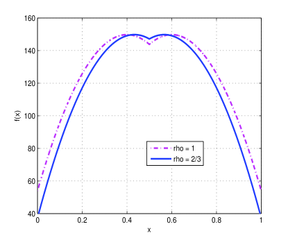
From the stopping condition (11), it can be seen that the stopping boundary is associated with the double-parabolic function f(x)=2ε2ln(ζδ)[14(|x12|ρε)2]𝑓𝑥2superscript𝜀2𝜁𝛿delimited-[]14superscript𝑥12𝜌𝜀2f(x)=\frac{2}{\varepsilon^{2}}\ln(\zeta\delta)\left[\frac{1}{4}-\left(\left|x-\frac{1}{2}\right|-\rho\varepsilon\right)^{2}\right] such that x𝑥x and f(x)𝑓𝑥f(x) correspond to the sample mean and sample size respectively. For ε=0.1,δ=0.05formulae-sequence𝜀0.1𝛿0.05\varepsilon=0.1,\;\delta=0.05 and ζ=1𝜁1\zeta=1, stopping boundaries with various ρ𝜌\rho are shown by Figure 1.

Refer to caption

Figure 1: Double-parabolic sampling

For fixed ε𝜀\varepsilon and δ𝛿\delta, the parameters ρ𝜌\rho and ζ𝜁\zeta affect the shape of the stoping boundary in a way as follows. As ρ𝜌\rho increases, the span of stopping boundary is increasing in the axis of sample mean. By decreasing ζ𝜁\zeta, the stopping boundary can be dragged toward the direction of increasing sample size. Hence, the parameter ρ𝜌\rho is referred to as the dilation coefficient. The parameter ζ𝜁\zeta is referred to as the coverage tuning parameter. Since the stopping boundary consists of two parabolas, this approach of estimating a binomial proportion is refereed to as the double-parabolic sequential estimation method.

4.1 Parametrization of the Sampling Scheme

In this section, we shall parameterize the double-parabolic sequential sampling scheme by the method described in Section 2.2. From the stopping condition (11), the stopping rule can be restated as: Continue sampling until 𝒟(𝒑^,n)=1𝒟subscript^𝒑subscript𝑛1\mathscr{D}(\widehat{\boldsymbol{p}}_{\ell},n_{\ell})=1 for some {1,,s}1𝑠\ell\in\{1,\cdots,s\}, where the function 𝒟(.,.)\mathscr{D}(.,.) is defined by

𝒟(z,n)={1if (|z12|ρε)214+ε2n2ln(ζδ),0otherwise𝒟𝑧𝑛cases1if (|z12|ρε)214+ε2n2ln(ζδ)0otherwise\mathscr{D}(z,n)=\begin{cases}1&\text{if {\small$(|z-\frac{1}{2}|-\rho\varepsilon)^{2}\geq\frac{1}{4}+\frac{\varepsilon^{2}n}{2\ln(\zeta\delta)}$}},\\ 0&\text{otherwise}\end{cases} (12)

Clearly, the function 𝒟(.,.)\mathscr{D}(.,.) associated with the double-parabolic sequential sampling scheme depends on the design parameters ρ,ζ,ε𝜌𝜁𝜀\rho,\zeta,\varepsilon and δ𝛿\delta. Applying the function 𝒟(.,.)\mathscr{D}(.,.) defined by (12) to (3) yields

Nmin=min{n:(|kn12|ρε)214+ε2n2ln(ζδ)for some nonnegative integer k not exceeding n}.subscript𝑁min:𝑛superscript𝑘𝑛12𝜌𝜀214superscript𝜀2𝑛2𝜁𝛿for some nonnegative integer k not exceeding nN_{\mathrm{min}}=\min\left\{n\in\mathbb{N}:\left(\left|\frac{k}{n}-\frac{1}{2}\right|-\rho\varepsilon\right)^{2}\geq\frac{1}{4}+\frac{\varepsilon^{2}n}{2\ln(\zeta\delta)}\;\text{for some nonnegative integer $k$ not exceeding $n$}\right\}. (13)

Since ε𝜀\varepsilon is usually small in practical applications, we restrict ε𝜀\varepsilon to satisfy 0<ρε140𝜌𝜀140<\rho\varepsilon\leq\frac{1}{4}. As a consequence of 0ρε140𝜌𝜀140\leq\rho\varepsilon\leq\frac{1}{4} and the fact that |z12|12𝑧1212\left|z-\frac{1}{2}\right|\leq\frac{1}{2} for any z[0,1]𝑧01z\in[0,1], it must be true that (|z12|ρε)2(12ρε)2superscript𝑧12𝜌𝜀2superscript12𝜌𝜀2\left(\left|z-\frac{1}{2}\right|-\rho\varepsilon\right)^{2}\leq\left(\frac{1}{2}-\rho\varepsilon\right)^{2} for any z[0,1]𝑧01z\in[0,1]. It follows from (13) that (12ρε)214+ε2Nmin2ln(ζδ)superscript12𝜌𝜀214superscript𝜀2subscript𝑁min2𝜁𝛿\left(\frac{1}{2}-\rho\varepsilon\right)^{2}\geq\frac{1}{4}+\frac{\varepsilon^{2}N_{\mathrm{min}}}{2\ln(\zeta\delta)}, which implies that the minimum sample size can be taken as

Nmin=2ρ(1ερ)ln1ζδ.subscript𝑁min2𝜌1𝜀𝜌1𝜁𝛿N_{\mathrm{min}}=\left\lceil 2\rho\left(\frac{1}{\varepsilon}-\rho\right)\ln\frac{1}{\zeta\delta}\right\rceil. (14)

On the other hand, applying the function 𝒟(.,.)\mathscr{D}(.,.) defined by (12) to (4) gives

Nmax=min{n:(|kn12|ρε)214+ε2n2ln(ζδ)for all nonnegative integer k not exceeding n}.subscript𝑁max:𝑛superscript𝑘𝑛12𝜌𝜀214superscript𝜀2𝑛2𝜁𝛿for all nonnegative integer k not exceeding nN_{\mathrm{max}}=\min\left\{n\in\mathbb{N}:\left(\left|\frac{k}{n}-\frac{1}{2}\right|-\rho\varepsilon\right)^{2}\geq\frac{1}{4}+\frac{\varepsilon^{2}n}{2\ln(\zeta\delta)}\;\text{for all nonnegative integer $k$ not exceeding $n$}\right\}. (15)

Since (|z12|ρε)20superscript𝑧12𝜌𝜀20\left(\left|z-\frac{1}{2}\right|-\rho\varepsilon\right)^{2}\geq 0 for any z[0,1]𝑧01z\in[0,1], it follows from (15) that 14+ε2Nmax2ln(ζδ)014superscript𝜀2subscript𝑁max2𝜁𝛿0\frac{1}{4}+\frac{\varepsilon^{2}N_{\mathrm{max}}}{2\ln(\zeta\delta)}\leq 0, which implies that maximum sample size can be taken as

Nmax=12ε2ln1ζδ.subscript𝑁max12superscript𝜀21𝜁𝛿N_{\mathrm{max}}=\left\lceil\frac{1}{2\varepsilon^{2}}\ln\frac{1}{\zeta\delta}\right\rceil. (16)

Therefore, the sample sizes n1,,nssubscript𝑛1subscript𝑛𝑠n_{1},\cdots,n_{s} can be chosen as functions of ρ,ζ,ε𝜌𝜁𝜀\rho,\zeta,\varepsilon and δ𝛿\delta which satisfy the following constraint:

Nminn1<<ns1<Nmaxns.subscript𝑁minsubscript𝑛1subscript𝑛𝑠1subscript𝑁maxsubscript𝑛𝑠N_{\mathrm{min}}\leq n_{1}<\cdots<n_{s-1}<N_{\mathrm{max}}\leq n_{s}. (17)

In particular, if the number of stages s𝑠s is given and the group sizes are expected to be approximately equal, then the sample sizes, n1,,nssubscript𝑛1subscript𝑛𝑠n_{1},\cdots,n_{s}, for all stages can be obtained by substituting Nminsubscript𝑁minN_{\mathrm{min}} defined by (14) and Nmaxsubscript𝑁maxN_{\mathrm{max}} defined by (16) into (5). For example, if the values of design parameters are ε=0.05,δ=0.05,ρ=34,ζ=2.6759formulae-sequence𝜀0.05formulae-sequence𝛿0.05formulae-sequence𝜌34𝜁2.6759\varepsilon=0.05,\;\delta=0.05,\;\rho=\frac{3}{4},\;\zeta=2.6759 and s=7𝑠7s=7, then the sample sizes of this sampling scheme are calculated as

n1=59,n2=116,n3=173,n4=231,n5=288,n6=345,n7=403.formulae-sequencesubscript𝑛159formulae-sequencesubscript𝑛2116formulae-sequencesubscript𝑛3173formulae-sequencesubscript𝑛4231formulae-sequencesubscript𝑛5288formulae-sequencesubscript𝑛6345subscript𝑛7403n_{1}=59,\;\;n_{2}=116,\;\;n_{3}=173,\;\;n_{4}=231,\;\;n_{5}=288,\;\;n_{6}=345,\;\;n_{7}=403.

The stopping rule is completely determined by substituting the values of design parameters into (11).

4.2 Uniform Controllability of Coverage Probability

Clearly, for pre-specified ε,δ𝜀𝛿\varepsilon,\;\delta and ρ𝜌\rho, the coverage probability Pr{|𝒑^p|<εp}Pr^𝒑𝑝bra𝜀𝑝\Pr\{|\widehat{\boldsymbol{p}}-p|<\varepsilon\mid p\} depends on the parameter ζ𝜁\zeta, the number of stages s𝑠s, and the sample sizes n1,,nssubscript𝑛1subscript𝑛𝑠n_{1},\cdots,n_{s}. As illustrated in Section 4.1, the number of stages s𝑠s and the sample sizes n1,,nssubscript𝑛1subscript𝑛𝑠n_{1},\cdots,n_{s} can be defined as functions of ζ(0,1δ)𝜁01𝛿\zeta\in(0,\frac{1}{\delta}). That is, the stopping rule can be parameterized by ζ𝜁\zeta. Accordingly, for any p(0,1)𝑝01p\in(0,1), the coverage probability Pr{|𝒑^p|<εp}Pr^𝒑𝑝bra𝜀𝑝\Pr\{|\widehat{\boldsymbol{p}}-p|<\varepsilon\mid p\} becomes a function of ζ𝜁\zeta. The following theorem shows that it suffices to choose ζ(0,1δ)𝜁01𝛿\zeta\in(0,\frac{1}{\delta}) small enough to guarantee the pre-specified confidence level.

Theorem 2

Let ε,δ(0,1)𝜀𝛿01\varepsilon,\;\delta\in(0,1) and ρ(0,1]𝜌01\rho\in(0,1] be fixed. Assume that the number of stages s𝑠s and the sample sizes n1,,nssubscript𝑛1subscript𝑛𝑠n_{1},\cdots,n_{s} are functions of ζ(0,1δ)𝜁01𝛿\zeta\in(0,\frac{1}{\delta}) such that the constraint (17) is satisfied. Then, Pr{|𝐩^p|<εp}Pr^𝐩𝑝bra𝜀𝑝\Pr\{|\widehat{\boldsymbol{p}}-p|<\varepsilon\mid p\} is no less than 1δ1𝛿1-\delta for any p(0,1)𝑝01p\in(0,1) provided that

0<ζ1δexp(lnδ2+ln[1exp(2ε2)]4ερ(1ρε)).0𝜁1𝛿𝛿212superscript𝜀24𝜀𝜌1𝜌𝜀0<\zeta\leq\frac{1}{\delta}\exp\left(\frac{\ln\frac{\delta}{2}+\ln\left[1-\exp(-2\varepsilon^{2})\right]}{4\varepsilon\rho(1-\rho\varepsilon)}\right).

See Appendix B for a proof. For Theorem 2 to be valid, the choice of sample sizes is very flexible. Specially, the sample sizes can be arithmetic or geometric progressions or any others, as long as the constraint (17) is satisfied. It can be seen that for the coverage probability to be uniformly controllable, the dilation coefficient ρ𝜌\rho must be greater than 00. Theorem 2 asserts that there exists ζ>0𝜁0\zeta>0 such that the coverage probability is no less than 1δ1𝛿1-\delta, regardless of the associated binomial proportion p𝑝p. For the purpose of reducing sampling cost, we want to have a value of ζ𝜁\zeta as large as possible such that the pre-specified confidence level is guaranteed for any p(0,1)𝑝01p\in(0,1). This can be accomplished by the technical components introduced in Sections 2.1, 2.3, 2.4 and Section 2.5. Clearly, for every value of ρ𝜌\rho, we can obtain a corresponding value of ζ𝜁\zeta (as large as possible) to ensure the desired confidence level. However, the performance of resultant stopping rules are different. Therefore, we can try a number of values of ρ𝜌\rho and pick the best resultant stopping rule for practical use.

4.3 Asymptotic Optimality of Sampling Schemes

Now we shall provide an important reason why we propose the sampling scheme of that structure by showing its asymptotic optimality. Since the performance of a group sampling scheme will be close to its fully sequential counterpart, we investigate the optimality of the fully sequential sampling scheme. In this scenario, the sample sizes n1,n2,,nssubscript𝑛1subscript𝑛2subscript𝑛𝑠n_{1},n_{2},\cdots,n_{s} are consecutive integers such that

2ρ(1ερ)ln1ζδ=n1<n2<<ns1<ns=12ε2ln1ζδ.2𝜌1𝜀𝜌1𝜁𝛿subscript𝑛1subscript𝑛2subscript𝑛𝑠1subscript𝑛𝑠12superscript𝜀21𝜁𝛿\left\lceil 2\rho\left(\frac{1}{\varepsilon}-\rho\right)\ln\frac{1}{\zeta\delta}\right\rceil=n_{1}<n_{2}<\cdots<n_{s-1}<n_{s}=\left\lceil\frac{1}{2\varepsilon^{2}}\ln\frac{1}{\zeta\delta}\right\rceil. (18)

The fully sequential sampling scheme can be viewed as a special case of a group sampling scheme of s=nsn1+1𝑠subscript𝑛𝑠subscript𝑛11s=n_{s}-n_{1}+1 stages and group size 111. Clearly, if δ,ζ𝛿𝜁\delta,\;\zeta and ρ𝜌\rho are fixed, the sampling scheme is dependent only on ε𝜀\varepsilon. Hence, for any p(0,1)𝑝01p\in(0,1), if we allow ε𝜀\varepsilon to vary in (0,1)01(0,1), then the coverage probability Pr{|𝒑^p|<εp}Pr^𝒑𝑝bra𝜀𝑝\Pr\{|\widehat{\boldsymbol{p}}-p|<\varepsilon\mid p\} and the average sample number 𝔼[𝐧]𝔼delimited-[]𝐧\mathbb{E}[\mathbf{n}] are functions of ε𝜀\varepsilon. We are interested in knowing the asymptotic behavior of these functions as ε0𝜀0\varepsilon\to 0, since ε𝜀\varepsilon is usually small in practical situations. The following theorem provides us the desired insights.

Theorem 3

Assume that δ(0,1),ζ(0,1δ)formulae-sequence𝛿01𝜁01𝛿\delta\in(0,1),\;\zeta\in(0,\frac{1}{\delta}) and ρ(0,1]𝜌01\rho\in(0,1] are fixed. Define N(p,ε,δ,ζ)=2p(1p)ln1ζδε2𝑁𝑝𝜀𝛿𝜁2𝑝1𝑝1𝜁𝛿superscript𝜀2N(p,\varepsilon,\delta,\zeta)=\frac{2p(1-p)\ln\frac{1}{\zeta\delta}}{\varepsilon^{2}} for p(0,1)𝑝01p\in(0,1) and ε(0,1)𝜀01\varepsilon\in(0,1). Then,

Pr{limε0𝐧N(p,ε,δ,ζ)=1p}=1,Prsubscript𝜀0𝐧𝑁𝑝𝜀𝛿𝜁conditional1𝑝1\displaystyle\Pr\left\{\lim_{\varepsilon\to 0}\frac{\mathbf{n}}{N(p,\varepsilon,\delta,\zeta)}=1\mid p\right\}=1,
limε0Pr{|𝒑^p|<εp}=2Φ(2ln1ζδ)1,subscript𝜀0Pr^𝒑𝑝bra𝜀𝑝2Φ21𝜁𝛿1\displaystyle\lim_{\varepsilon\to 0}\Pr\{|\widehat{\boldsymbol{p}}-p|<\varepsilon\mid p\}=2\Phi\left(\sqrt{2\ln\frac{1}{\zeta\delta}}\right)-1, (19)
limε0𝔼[𝐧]N(p,ε,δ,ζ)=1subscript𝜀0𝔼delimited-[]𝐧𝑁𝑝𝜀𝛿𝜁1\displaystyle\lim_{\varepsilon\to 0}\frac{\mathbb{E}[\mathbf{n}]}{N(p,\varepsilon,\delta,\zeta)}=1 (20)

for any p(0,1)𝑝01p\in(0,1).

See Appendix C for a proof. From (19), it can be seen that limε0Pr{|𝒑^p|<εp}=1δsubscript𝜀0Pr^𝒑𝑝bra𝜀𝑝1𝛿\lim_{\varepsilon\to 0}\Pr\{|\widehat{\boldsymbol{p}}-p|<\varepsilon\mid p\}=1-\delta for any p(0,1)𝑝01p\in(0,1) if ζ=1δexp(12𝒵δ/22)𝜁1𝛿12superscriptsubscript𝒵𝛿22\zeta=\frac{1}{\delta}\exp(-\frac{1}{2}\mathcal{Z}_{\delta/2}^{2}). Such value can be taken as an initial value for the coverage tuning parameter ζ𝜁\zeta. In addition to provide guidance on the coverage tuning techniques, Theorem 3 also establishes the optimality of the sampling scheme. To see this, let 𝒩(p,ε,δ)𝒩𝑝𝜀𝛿\mathscr{N}(p,\varepsilon,\delta) denote the minimum sample size n𝑛n required for a fixed-sample-size procedure to guarantee that Pr{|X¯np|<εp}1δPrsubscript¯𝑋𝑛𝑝bra𝜀𝑝1𝛿\Pr\{|\overline{X}_{n}-p|<\varepsilon\mid p\}\geq 1-\delta for any p(0,1)𝑝01p\in(0,1), where X¯n=i=1nXinsubscript¯𝑋𝑛superscriptsubscript𝑖1𝑛subscript𝑋𝑖𝑛\overline{X}_{n}=\frac{\sum_{i=1}^{n}X_{i}}{n}. It is well known that from the central limit theorem,

limε0𝒩(p,ε,δ)p(1p)(𝒵δ/2ε)2=1.subscript𝜀0𝒩𝑝𝜀𝛿𝑝1𝑝superscriptsubscript𝒵𝛿2𝜀21\lim_{\varepsilon\to 0}\frac{\mathscr{N}(p,\varepsilon,\delta)}{p(1-p)\left(\frac{\mathcal{Z}_{\delta/2}}{\varepsilon}\right)^{2}}=1. (21)

Making use of (20), (21) and letting ζ=1δexp(12𝒵δ/22)𝜁1𝛿12superscriptsubscript𝒵𝛿22\zeta=\frac{1}{\delta}\exp(-\frac{1}{2}\mathcal{Z}_{\delta/2}^{2}), we have limε0𝒩(p,ε,δ)N(p,ε,δ,ζ)=1subscript𝜀0𝒩𝑝𝜀𝛿𝑁𝑝𝜀𝛿𝜁1\lim_{\varepsilon\to 0}\frac{\mathscr{N}(p,\varepsilon,\delta)}{N(p,\varepsilon,\delta,\zeta)}=1 for p(0,1)𝑝01p\in(0,1) and δ(0,1)𝛿01\delta\in(0,1), which implies the asymptotic optimality of the double-parabolic sampling scheme. By virtue of (20), an approximate formula for computing the average sample number is given as

𝔼[𝐧]N(p,ε,δ,ζ)=2p(1p)ln1ζδε2𝔼delimited-[]𝐧𝑁𝑝𝜀𝛿𝜁2𝑝1𝑝1𝜁𝛿superscript𝜀2\mathbb{E}[\mathbf{n}]\approx N(p,\varepsilon,\delta,\zeta)=\frac{2p(1-p)\ln\frac{1}{\zeta\delta}}{\varepsilon^{2}} (22)

for p(0,1)𝑝01p\in(0,1) and ε(0,1)𝜀01\varepsilon\in(0,1). From (21), one obtains 𝒩(p,ε,δ)p(1p)(𝒵δ/2ε)2𝒩𝑝𝜀𝛿𝑝1𝑝superscriptsubscript𝒵𝛿2𝜀2\mathscr{N}(p,\varepsilon,\delta)\approx p(1-p)\left(\frac{\mathcal{Z}_{\delta/2}}{\varepsilon}\right)^{2}, which is a well-known result in statistics. In situations that no information of p𝑝p is available, one usually uses

Nnormal=def14(𝒵δ/2ε)2superscriptdefsubscript𝑁normal14superscriptsubscript𝒵𝛿2𝜀2N_{\mathrm{normal}}\stackrel{{\scriptstyle\mathrm{def}}}{{=}}\left\lceil\frac{1}{4}\left(\frac{\mathcal{Z}_{\delta/2}}{\varepsilon}\right)^{2}\right\rceil (23)

as the sample size for estimating the binomial proportion p𝑝p with prescribed margin of error ε𝜀\varepsilon and confidence level 1δ1𝛿1-\delta. Since the sample size formula (23) can lead to under-coverage, researchers in many areas are willing to use a more conservative but rigorous sample size formula

Nch=defln2δ2ε2,superscriptdefsubscript𝑁ch2𝛿2superscript𝜀2N_{\mathrm{ch}}\stackrel{{\scriptstyle\mathrm{def}}}{{=}}\left\lceil\frac{\ln\frac{2}{\delta}}{2\varepsilon^{2}}\right\rceil, (24)

which is derived from the Chernoff-Hoeffding bound [3, 26]. Comparing (22) and (24), one can see that under the premise of guaranteeing the prescribed confidence level 1δ1𝛿1-\delta, the double-parabolic sampling scheme can lead to a substantial reduction of sample number when the unknown binomial proportion p𝑝p is close to 00 or 111.

4.4 Bounds on Distribution and Expectation of Sample Number

We shall derive analytic bounds for the cumulative distribution function and expectation of the sample number 𝐧𝐧\mathbf{n} associated with the double-parabolic sampling scheme. In this direction, we have obtained the following results.

Theorem 4

Let p(0,12]𝑝012p\in(0,\frac{1}{2}]. Define a=12ρε14+ε2n2ln(ζδ)subscript𝑎12𝜌𝜀14superscript𝜀2subscript𝑛2𝜁𝛿a_{\ell}=\frac{1}{2}-\rho\varepsilon-\sqrt{\frac{1}{4}+\frac{\varepsilon^{2}n_{\ell}}{2\ln(\zeta\delta)}} for =1,,s1𝑠\ell=1,\cdots,s. Let τ𝜏\tau denote the index of stage such that aτ1p<aτsubscript𝑎𝜏1𝑝subscript𝑎𝜏a_{\tau-1}\leq p<a_{\tau}. Then, Pr{𝐧>np}exp(n(a,p))Pr𝐧conditionalsubscript𝑛𝑝subscript𝑛subscript𝑎𝑝\Pr\{\mathbf{n}>n_{\ell}\mid p\}\leq\exp(n_{\ell}\mathscr{M}(a_{\ell},p)) for τ<s𝜏𝑠\tau\leq\ell<s. Moreover, 𝔼[𝐧]nτ+=τs1(n+1n)exp(n(a,p))𝔼delimited-[]𝐧subscript𝑛𝜏superscriptsubscript𝜏𝑠1subscript𝑛1subscript𝑛subscript𝑛subscript𝑎𝑝\mathbb{E}[\mathbf{n}]\leq n_{\tau}+\sum_{\ell=\tau}^{s-1}(n_{\ell+1}-n_{\ell})\exp(n_{\ell}\mathscr{M}(a_{\ell},p)).

See Appendix D for a proof. By the symmetry of the double-parabolic sampling scheme, similar analytic bounds for the distribution and expectation of the sample number can be derived for the case that p[12,1)𝑝121p\in[\frac{1}{2},1).

5 Comparison of Computational Methods

In this section, we shall compare various computational methods. First, we will illustrate why a frequently-used method of evaluating the coverage probability based on gridding the parameter space is not rigorous and is less efficient as compared to the Adapted B&B Algorithm. Second, we will introduce the Adaptive Maximum Checking Algorithm of [10] which has better computational efficiency as compared to the Adapted B&B Algorithm. Third, we will explain that it is more advantageous in terms of numerical accuracy to work with the complementary coverage probability as compared to direct evaluation of the coverage probability. Finally, we will compare the computational methods of Chen [7, 9, 11, 13, 14] and Frey [23] for the design of sequential procedures for estimating a binomial proportion.

5.1 Verifying Coverage Guarantee without Gridding Parameter Space

For purpose of constructing a sampling scheme so that the prescribed confidence level 1δ1𝛿1-\delta is guaranteed, an essential task is to determine whether the coverage probability Pr{|𝒑^p|<εp}Pr^𝒑𝑝bra𝜀𝑝\Pr\{|\widehat{\boldsymbol{p}}-p|<\varepsilon\mid p\} associated with a given stopping rule is no less than 1δ1𝛿1-\delta. In other words, it is necessary to compare the infimum of coverage probability with 1δ1𝛿1-\delta. To accomplish such a task of checking coverage guarantee, a natural method is to evaluate the infimum of coverage probability as follows:

(i): Choose m𝑚m grid points p1,,pmsubscript𝑝1subscript𝑝𝑚p_{1},\cdots,p_{m} from parameter space (0,1)01(0,1).

(ii): Compute cj=Pr{|𝒑^p|<εpj}subscript𝑐𝑗Pr^𝒑𝑝bra𝜀subscript𝑝𝑗c_{j}=\Pr\{|\widehat{\boldsymbol{p}}-p|<\varepsilon\mid p_{j}\} for j=1,,m𝑗1𝑚j=1,\cdots,m.

(iii): Take min{c1,,cm}subscript𝑐1subscript𝑐𝑚\min\{c_{1},\cdots,c_{m}\} as infp(0,1)Pr{|𝒑^p|<εp}subscriptinfimum𝑝01Pr^𝒑𝑝bra𝜀𝑝\inf_{p\in(0,1)}\Pr\{|\widehat{\boldsymbol{p}}-p|<\varepsilon\mid p\}.

This method can be easily mistaken as an exact approach and has been frequently used for evaluating coverage probabilities in many problem areas.

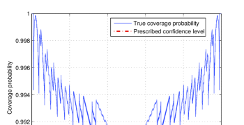
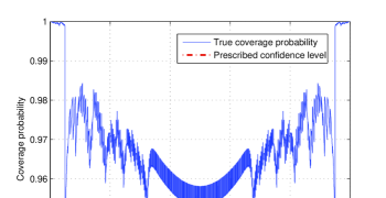
It is not hard to show that if the sample size 𝐧𝐧\mathbf{n} of a sequential procedure has a support 𝒮𝒮\mathscr{S}, then the coverage probability Pr{|𝒑^p|<εp}Pr^𝒑𝑝bra𝜀𝑝\Pr\{|\widehat{\boldsymbol{p}}-p|<\varepsilon\mid p\} is discontinuous at p𝒫(0,1)𝑝𝒫01p\in\mathscr{P}\cap(0,1), where 𝒫={kn±ε:k is a nonnegative integer\mathscr{P}=\{\frac{k}{n}\pm\varepsilon:\text{$k$ is a nonnegative integer} no greater than n𝒮}\text{no greater than $n\in\mathscr{S}$}\}. The set 𝒫𝒫\mathscr{P} typically has a large number of parameter values. Due to the discontinuity of the coverage probability as a function of p𝑝p, the coverage probabilities can differ significantly for two parameter values which are extremely close. This implies that an intolerable error can be introduced by taking the minimum of coverage probabilities of a finite number of parameter values as the infimum of coverage probability on the whole parameter space. So, if one simply uses the minimum of the coverage probabilities of a finite number of parameter values as the infimum of coverage probability to check the coverage guarantee, the sequential estimator 𝒑^^𝒑\widehat{\boldsymbol{p}} of the resultant stopping rule will fail to guarantee the prescribed confidence level.

In addition to the lack of rigorousness, another drawback of checking coverage guarantee based on the method of gridding parameter space is its low efficiency. A critical issue is on the choice of the number, m𝑚m, of grid points. If the number m𝑚m is too small, the induced error can be substantial. On the other hand, choosing a large number for m𝑚m results in high computational complexity.

In contrast to the method based on gridding parameter space, the Adapted B&B Algorithm is a rigorous approach for checking coverage guarantee as a consequence of the mechanism for comparing the bounds of coverage probability with the prescribed confidence level. The algorithm is also efficient due to the mechanism of pruning branches.

5.2 Adaptive Maximum Checking Algorithm

As illustrated in Section 2, the techniques developed in [7, 9, 11, 13, 14] are sufficient to provide exact solutions for a wide range of sequential estimation problems. However, one of the four components, the Adapted B&B Algorithm, requires computing both the lower and upper bounds of the complementary coverage probability. To further reduce the computational complexity, it is desirable to have a checking algorithm which needs only one of the lower and upper bounds. For this purpose, Chen had developed the Adaptive Maximum Checking Algorithm (AMCA) in [10, Section 3.3] and [15, Section 2.7]. In the following introduction of the AMCA, we shall follow the description of [10]. The AMCA can be applied to a wide class of computational problems dependent on the following critical subroutine:

Determine whether a function C(θ)𝐶𝜃C(\theta) is smaller than a prescribed number δ𝛿\delta for every value of θ𝜃\theta contained in interval [θ¯,θ¯]¯𝜃¯𝜃[\underline{\theta},\overline{\theta}].

Specially, for checking the coverage guarantee in the context of estimating a binomial proportion, the parameter θ𝜃\theta is the binomial proportion p𝑝p and the function C(θ)𝐶𝜃C(\theta) is actually the complementary coverage probability. In many situations, it is impossible or very difficult to evaluate C(θ)𝐶𝜃C(\theta) for every value of θ𝜃\theta in interval [θ¯,θ¯]¯𝜃¯𝜃[\underline{\theta},\overline{\theta}], since the interval may contain infinitely many or an extremely large number of values. Similar to the Adapted B&B Algorithm, the purpose of AMCA is to reduce the computational complexity associated with the problem of determining whether the maximum of C(θ)𝐶𝜃C(\theta) over [θ¯,θ¯]¯𝜃¯𝜃[\underline{\theta},\overline{\theta}] is less than δ𝛿\delta. The only assumption required for AMCA is that, for any interval [a,b][θ¯,θ¯]𝑎𝑏¯𝜃¯𝜃[a,b]\subseteq[\underline{\theta},\overline{\theta}], it is possible to compute an upper bound C¯(a,b)¯𝐶𝑎𝑏\overline{C}(a,b) such that C(θ)C¯(a,b)𝐶𝜃¯𝐶𝑎𝑏C(\theta)\leq\overline{C}(a,b) for any θ[a,b]𝜃𝑎𝑏\theta\in[a,b] and that the upper bound converges to C(θ)𝐶𝜃C(\theta) as the interval width ba𝑏𝑎b-a tends to 00. The backward AMCA proceeds as follows:


Choose initial step size d>ηChoose initial step size d>η\nabla\;\text{Choose initial step size $d>\eta$}.
Let F0,T0 and bθ¯Let F0,T0 and bθ¯\nabla\;\text{Let $F\leftarrow 0,\;T\leftarrow 0$ and $b\leftarrow\overline{\theta}$}.
While F=T=0, do the followingWhile F=T=0, do the following\nabla\;\text{While $F=T=0$, do the following}:
Let st0 and 2Let st0 and 2\indent\indent\;\diamond\;\text{Let $\text{st}\leftarrow 0$ and $\ell\leftarrow 2$};
While st=0, do the followingWhile st=0, do the following\indent\indent\;\diamond\;\text{While $\text{st}=0$, do the following}:
Let 1 and dd2absentLet 1 and dd2\indent\indent\indent\indent\;\star\;\text{Let $\ell\leftarrow\ell-1$ and $d\leftarrow d2^{\ell}$}.
If bd>θ¯, then let abd and T0absentIf bd>θ¯, then let abd and T0\indent\indent\indent\indent\;\star\;\text{If $b-d>\underline{\theta}$, then let $a\leftarrow b-d$ and $T\leftarrow 0$}.
      Otherwise, let aθ¯𝑎¯𝜃a\leftarrow\underline{\theta} and T1𝑇1T\leftarrow 1.
If C¯(a,b)<δ, then let st1 and baabsentIf C¯(a,b)<δ, then let st1 and ba\indent\indent\indent\indent\;\star\;\text{If $\overline{C}(a,b)<\delta$, then let $\text{st}\leftarrow 1$ and $b\leftarrow a$}.
If d<η, then let st1 and F1absentIf d<η, then let st1 and F1\indent\indent\indent\indent\;\star\;\text{If $d<\eta$, then let $\text{st}\leftarrow 1$ and $F\leftarrow 1$}.
Return FReturn F\nabla\;\text{Return $F$}.

The output of the backward AMCA is a binary variable F𝐹F such that “F=0𝐹0F=0” means “C(θ)<δ𝐶𝜃𝛿C(\theta)<\delta” and “F=1𝐹1F=1” means “C(θ)δ𝐶𝜃𝛿C(\theta)\geq\delta”. An intermediate variable T𝑇T is introduced in the description of AMCA such that “T=1𝑇1T=1” means that the left endpoint of the interval is reached. The backward AMCA starts from the right endpoint of the interval (i.e., b=θ¯𝑏¯𝜃b=\overline{\theta}) and attempts to find an interval [a,b]𝑎𝑏[a,b] such that C¯(a,b)<δ¯𝐶𝑎𝑏𝛿\overline{C}(a,b)<\delta. If such an interval is available, then, attempt to go backward to find the next consecutive interval with twice width. If doubling the interval width fails to guarantee C¯(a,b)<δ¯𝐶𝑎𝑏𝛿\overline{C}(a,b)<\delta, then try to repeatedly cut the interval width in half to ensure that C¯(a,b)<δ¯𝐶𝑎𝑏𝛿\overline{C}(a,b)<\delta. If the interval width becomes smaller than a prescribed tolerance η𝜂\eta, then AMCA declares that “F=1𝐹1F=1”. For our relevant statistical problems, if C(θ)δ𝐶𝜃𝛿C(\theta)\geq\delta for some θ[θ¯,θ¯]𝜃¯𝜃¯𝜃\theta\in[\underline{\theta},\overline{\theta}], it is sure that “F=1𝐹1F=1” will be declared. On the other hand, it is possible that “F=1𝐹1F=1” is declared even though C(θ)<δ𝐶𝜃𝛿C(\theta)<\delta for any θ[θ¯,θ¯]𝜃¯𝜃¯𝜃\theta\in[\underline{\theta},\overline{\theta}]. However, such situation can be made extremely rare and immaterial if we choose η𝜂\eta to be a very small number. Moreover, this will only introduce negligible conservativeness in the evaluation of C(θ)𝐶𝜃C(\theta) if η𝜂\eta is chosen to be sufficiently small (e.g., η=1015𝜂superscript1015\eta=10^{-15}). Clearly, the backward AMCA can be easily modified as forward AMCA. Moreover, the AMCA can also be easily modified as Adaptive Minimum Checking Algorithm (forward and backward). For checking the maximum of complementary coverage probability Pr{|𝒑^p|εp}Pr^𝒑𝑝conditional𝜀𝑝\Pr\{|\widehat{\boldsymbol{p}}-p|\geq\varepsilon\mid p\}, one can use the AMCA with C(p)=Pr{|𝒑^p|εp}𝐶𝑝Pr^𝒑𝑝conditional𝜀𝑝C(p)=\Pr\{|\widehat{\boldsymbol{p}}-p|\geq\varepsilon\mid p\} over interval [0,12]012[0,\frac{1}{2}]. We would like to point out that, in contrast to the Adapted B&B Algorithm, it seems difficult to generalize the AMCA to problems involving multidimensional parameter spaces.

5.3 Working with Complementary Coverage Probability

We would like to point out that, instead of evaluating the coverage probability as in [23], it is better to evaluate the complementary coverage probability for purpose of reducing numerical error. The advantage of working on the complementary coverage probability can be explained as follows: Note that, in many cases, the coverage probability is very close to 111 and the complementary coverage probability is very close to 00. Since the absolute precision for computing a number close to 111 is much lower than the absolute precision for computing a number close to 00, the method of directly evaluating the coverage probability will lead to intolerable numerical error for problems involving small δ𝛿\delta. As an example, consider a situation that the complementary coverage probability is in the order of 105superscript10510^{-5}. Direct computation of the coverage probability can easily lead to an absolute error of the order of 105superscript10510^{-5}. However, the absolute error of computing the complementary coverage probability can be readily controlled at the order of 109superscript10910^{-9}.

5.4 Comparison of Approaches of Chen and J. Frey

As mentioned in the introduction, J. Frey published a paper [23] in The American Statistician (TAS) on the sequential estimation of a binomial proportion with prescribed margin of error and confidence level. The approaches of Chen and Frey are based on the same strategy as follows: First, construct a family of stopping rules parameterized by γ𝛾\gamma (and possibly other design parameters) so that the associated coverage probability Pr{|𝒑^p|<εp}Pr^𝒑𝑝bra𝜀𝑝\Pr\{|\widehat{\boldsymbol{p}}-p|<\varepsilon\mid p\} can be controlled by parameter γ𝛾\gamma in the sense that the coverage probability can be made arbitrarily close to 111 by increasing γ𝛾\gamma. Second, adaptively and rigorously check the coverage guarantee by virtue of bounds of coverage probabilities. Third, apply a bisection search method to determine the parameter γ𝛾\gamma so that the coverage probability is no less than the prescribed confidence level 1δ1𝛿1-\delta for any p(0,1)𝑝01p\in(0,1).

For the purpose of controlling the coverage probability, Frey [23] applied the inclusion principle previously proposed in [14, Section 3] and used in [7, 9, 11, 13]. As illustrated in Section 3, the central idea of inclusion principle is to use a sequence of confidence intervals to construct stopping rules so that the sampling process is continued until a confidence interval is included by an interval defined in terms of the estimator and margin of error. Due to the inclusion relationship, the associated coverage probability can be controlled by the confidence coefficients of the sequence of confidence intervals. The critical value γ𝛾\gamma used by Frey plays the same role for controlling coverage probabilities as that of the coverage tuning parameter ζ𝜁\zeta used by Chen. Frey [23] stated stopping rules in terms of confidence limits. This way of expressing stopping rules is straightforward and insightful, since one can readily seen the principle behind the construction. For convenience of practical use, Chen proposed to eliminate the necessity of computing confidence limits.

Frey’s method for checking coverage guarantee differs from the Adapted B&B Algorithm, but coincides with other techniques of Chen [10]. On September 18, 2011, in response to an inquiry on the coincidence of the research results, Frey simultaneously emailed Xinjia Chen (the coauthor of the present paper) and TAS Editor John Stufken all pre-final revisions of his manuscript for the paper [23]. In his original manuscript submitted to TAS in July 2009, Frey’s method was to “simply approximate CP(γ)𝐶𝑃𝛾CP(\gamma) by taking the minimum over the grid of values p=1/2001,,2000/2001𝑝1200120002001p=1/2001,...,2000/2001.” In the first revision of his manuscript submitted to TAS in November 2009, Frey’s method was to “approximate CP(γ)𝐶𝑃𝛾CP(\gamma) by taking the minimum of T(p;γ)𝑇𝑝𝛾T(p;\gamma) over the grid of values p=1/2001,,2000/2001𝑝1200120002001p=1/2001,...,2000/2001 and the set of values of the form p=c±ϵ𝑝plus-or-minus𝑐italic-ϵp=c\pm\epsilon, where cC𝑐𝐶c\in C and ϵ=1010italic-ϵsuperscript1010\epsilon=10^{-10}.” In Frey’s notational system, γ𝛾\gamma is the critical value which plays the same role as that of the coverage tuning parameter ζ𝜁\zeta in the present paper, T(p;γ)𝑇𝑝𝛾T(p;\gamma) is the coverage probability, CP(γ)𝐶𝑃𝛾CP(\gamma) is the infimum of coverage probability for p(0,1)𝑝01p\in(0,1), and C={p^±ε: p^ is a possible value of 𝒑^}(0,1)𝐶conditional-setplus-or-minus^𝑝𝜀 p^ is a possible value of 𝒑^01C=\{\widehat{p}\pm\varepsilon:\text{ $\widehat{p}$ is a possible value of $\widehat{\boldsymbol{p}}$}\}\cap(0,1). From the original and the first revision of his manuscript submitted to TAS before April 2010, it can be seen that Frey’s method of checking coverage guarantee was dependent on taking the minimum of coverage probabilities for a finite number of gridding points of p(0,1)𝑝01p\in(0,1) as the infimum coverage probability for p(0,1)𝑝01p\in(0,1). As can be seen from Section 5.1 of the present paper, such method lacks rigorousness and efficiency. In the second revision of his manuscript submitted to TAS in April 2010, for the purpose of checking coverage guarantee, Frey replaced the method of gridding parameter space with an interval bounding technique and proposed a checking algorithm which is essentially the same as the AMCA precedentially established by Chen [10, Section 3.3] in November 2009.

Similar to the AMCA of [10, Section 3.3], the algorithm of Frey [23, Appendix] for checking coverage guarantee adaptively scans the parameter space based on interval bounding. The adaptive method used by Frey for updating step size is essentially the same as that of the AMCA. Ignoring the number 0.010.010.01 in Frey’s expression “ϵi=min{0.01,2(pi1pi2)}subscriptitalic-ϵ𝑖0.012subscript𝑝𝑖1subscript𝑝𝑖2\epsilon_{i}=\min\{0.01,2(p_{i-1}-p_{i-2})\}”, which has very little impact on the computational efficiency, Frey’s step size ϵisubscriptitalic-ϵ𝑖\epsilon_{i} can be identified as the adaptive step size d𝑑d in the AMCA. The operation associated with “ϵi=min{0.01,2(pi1pi2)}subscriptitalic-ϵ𝑖0.012subscript𝑝𝑖1subscript𝑝𝑖2\epsilon_{i}=\min\{0.01,2(p_{i-1}-p_{i-2})\}” has a similar function as that of the command “Let st0st0\text{st}\leftarrow 0 and 22\ell\leftarrow 2” in the outer loop of the AMCA. The operation associated with Frey’s expression “pi1+ϵi/2j,j0subscript𝑝𝑖1subscriptitalic-ϵ𝑖superscript2𝑗𝑗0p_{i-1}+\epsilon_{i}/2^{j},\;j\geq 0” is equivalent to that of the command “Let 11\ell\leftarrow\ell-1 and dd2𝑑𝑑superscript2d\leftarrow d2^{\ell}” in the inner loop of the AMCA. Frey proposed to declare a failure of coverage guarantee if “the distance from pi1subscript𝑝𝑖1p_{i-1} to the candidate value for pisubscript𝑝𝑖p_{i} falls below 1014superscript101410^{-14}”. The number “1014superscript101410^{-14}” actually plays the same role as “η𝜂\eta” in the AMCA, where “η=1015𝜂superscript1015\eta=10^{-15}” is recommended by [10].

6 Numerical Results

In this section, we shall illustrate the proposed double-parabolic sampling scheme through examples. As demonstrated in Section 2.2 and Section 4, the double-parabolic sampling scheme can be parameterized by the dilation coefficient ρ𝜌\rho and the coverage tuning parameter ζ𝜁\zeta. Hence, the performance of the resultant stopping rule can be optimized with respect to ρ(0,1]𝜌01\rho\in(0,1] and ζ𝜁\zeta by choosing various values of ρ𝜌\rho from interval (0,1]01(0,1] and determining the corresponding values of ζ𝜁\zeta by the computational techniques introduced in Section 2 to guarantee the desired confidence interval.

6.1 Asymptotic Analysis May Be Inadequate

For fully sequential cases, we have evaluated the double-parabolic sampling scheme with ε=0.1,δ=0.05,ρ=0.1formulae-sequence𝜀0.1formulae-sequence𝛿0.05𝜌0.1\varepsilon=0.1,\;\delta=0.05,\;\rho=0.1 and ζ=1δexp(12𝒵δ/22)2.93𝜁1𝛿12superscriptsubscript𝒵𝛿222.93\zeta=\frac{1}{\delta}\exp\left(-\frac{1}{2}\mathcal{Z}_{\delta/2}^{2}\right)\approx 2.93. The stopping boundary is displayed in the left side of Figure 2. The function of coverage probability with respect to the binomial proportion is shown in the right side of Figure 2, which indicates that the coverage probabilities are generally substantially lower than the prescribed confidence level 1δ=0.051𝛿0.051-\delta=0.05. By considering ε=0.1𝜀0.1\varepsilon=0.1 as a small number and applying the asymptotic theory, the coverage probability associated with the sampling scheme is expected to be close to 0.950.950.95. This numerical example demonstrates that although the asymptotic method is insightful and involves virtually no computation, it may not be adequate.

In general, the main drawback of an asymptotic method is that there is no guarantee of coverage probability. Although an asymptotical method asserts that if the margin of error ε𝜀\varepsilon tends to 00, the coverage probability will tend to the pre-specified confidence level 1δ1𝛿1-\delta, it is difficult to determine how small the margin of error ε𝜀\varepsilon is sufficient for the asymptotic method to be applicable. Note that ε0𝜀0\varepsilon\to 0 implies the average sample size tends to \infty. However, in reality, the sample sizes must be finite. Consequently, an asymptotic method inevitably introduces unknown statistical error. Since an asymptotic method does not necessarily guarantee the prescribed confidence level, it is not fair to compare its associated sample size with that of an exact method, which guarantees the pre-specified confidence level.

This example also indicates that, due to the discrete nature of the problem, the coverage probability is a discontinuous and erratic function of p𝑝p, which implies that Monte Carlo simulation is not suitable for evaluating the coverage performance.
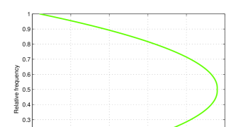
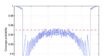


Refer to caption
Refer to caption
Figure 2: Double-parabolic sampling with ε=0.1,δ=0.05,ρ=110formulae-sequence𝜀0.1formulae-sequence𝛿0.05𝜌110\varepsilon=0.1,\;\delta=0.05,\;\rho=\frac{1}{10} and ζ=2.93𝜁2.93\zeta=2.93

6.2 Parametric Values of Fully Sequential Schemes

For fully sequential cases, to allow direct application of our double-parabolic sequential method, we have obtained values of coverage tuning parameter ζ𝜁\zeta, which guarantee the prescribed confidence levels, for double-parabolic sampling schemes with ρ=34𝜌34\rho=\frac{3}{4} and various combinations of (ε,δ)𝜀𝛿(\varepsilon,\delta) as shown in Table 1. We used the computational techniques introduced in Section 2 to obtain this table.

Table 1: Coverage Tuning Parameter
ε𝜀\varepsilon δ𝛿\delta ζ𝜁\zeta ε𝜀\varepsilon δ𝛿\delta ζ𝜁\zeta ε𝜀\varepsilon δ𝛿\delta ζ𝜁\zeta
0.10.10.1 0.10.10.1 2.04272.04272.0427 0.10.10.1 0.050.050.05 2.41742.41742.4174 0.10.10.1 0.010.010.01 3.06083.06083.0608
0.050.050.05 0.10.10.1 2.05032.05032.0503 0.050.050.05 0.050.050.05 2.58622.58622.5862 0.050.050.05 0.010.010.01 3.31253.31253.3125
0.020.020.02 0.10.10.1 2.17252.17252.1725 0.020.020.02 0.050.050.05 2.55922.55922.5592 0.020.020.02 0.010.010.01 3.44613.44613.4461
0.010.010.01 0.10.10.1 2.17252.17252.1725 0.010.010.01 0.050.050.05 2.55922.55922.5592 0.010.010.01 0.010.010.01 3.44613.44613.4461

To illustrate the use of Table 1, suppose that one wants a fully sequential sampling procedure to ensure that Pr{|𝒑^p|<0.1p}>0.95Pr^𝒑𝑝bra0.1𝑝0.95\Pr\{|\widehat{\boldsymbol{p}}-p|<0.1\mid p\}>0.95 for any p(0,1)𝑝01p\in(0,1). This means that one can choose ε=0.1,δ=0.05formulae-sequence𝜀0.1𝛿0.05\varepsilon=0.1,\;\delta=0.05 and the range of sample size is given by (18). From Table 1, it can be seen that the value of ζ𝜁\zeta corresponding to ε=0.1,δ=0.05formulae-sequence𝜀0.1𝛿0.05\varepsilon=0.1,\;\delta=0.05 is 2.41742.41742.4174. Consequently, the stopping rule is completely determined by substituting the values of design parameters ε=0.1,δ=0.05,ρ=34,ζ=2.4174formulae-sequence𝜀0.1formulae-sequence𝛿0.05formulae-sequence𝜌34𝜁2.4174\varepsilon=0.1,\;\delta=0.05,\;\rho=\frac{3}{4},\;\zeta=2.4174 into its definition. The stopping boundary of this sampling scheme is displayed in the left side of Figure 3. The function of coverage probability with respect to the binomial proportion is shown in the right side of Figure 3.
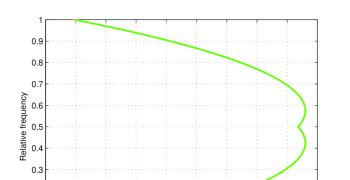
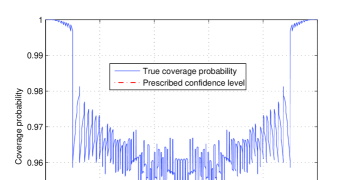

Refer to caption
Refer to caption
Figure 3: Double-parabolic sampling with ε=0.1,δ=0.05,ρ=34formulae-sequence𝜀0.1formulae-sequence𝛿0.05𝜌34\varepsilon=0.1,\;\delta=0.05,\;\rho=\frac{3}{4} and ζ=2.4174𝜁2.4174\zeta=2.4174

6.3 Parametric Values of Group Sequential Schemes

In many situations, especially in clinical trials, it is desirable to use group sequential sampling schemes. In Tables 2 and 3, assuming that sample sizes satisfy (5) for the purpose of having approximately equal group sizes, we have obtained parameters for concrete schemes by the computational techniques introduced in Section 2.

For dilation coefficient ρ=34𝜌34\rho=\frac{3}{4} and confidence parameter δ=0.05𝛿0.05\delta=0.05, we have obtained values of coverage tuning parameter ζ𝜁\zeta, which guarantee the prescribed confidence level 0.950.950.95, for double-parabolic sampling schemes, with the number of stages s𝑠s ranging from 333 to 101010, as shown in Table 2.

For dilation coefficient ρ=34𝜌34\rho=\frac{3}{4} and confidence parameter δ=0.01𝛿0.01\delta=0.01, we have obtained values of coverage tuning parameter ζ𝜁\zeta, which guarantee the prescribed confidence level 0.990.990.99, for double-parabolic sampling schemes, with the number of stages s𝑠s ranging from 333 to 101010, as shown in Table 3.

Table 2: Coverage Tuning Parameter
s=3𝑠3s=3 s=4𝑠4s=4 s=5𝑠5s=5 s=6𝑠6s=6 s=7𝑠7s=7 s=8𝑠8s=8 s=9𝑠9s=9 s=10𝑠10s=10
ε=0.1𝜀0.1\varepsilon=0.1 2.65832.65832.6583 2.65832.65832.6583 2.50962.50962.5096 2.59462.59462.5946 2.44592.44592.4459 2.65122.65122.6512 2.50962.50962.5096 2.44592.44592.4459
ε=0.05𝜀0.05\varepsilon=0.05 2.67592.67592.6759 2.67592.67592.6759 2.67592.67592.6759 2.67592.67592.6759 2.67592.67592.6759 2.67592.67592.6759 2.67592.67592.6759 2.67592.67592.6759
ε=0.02𝜀0.02\varepsilon=0.02 2.67252.67252.6725 2.67252.67252.6725 2.67252.67252.6725 2.67252.67252.6725 2.67252.67252.6725 2.67252.67252.6725 2.67252.67252.6725 2.67252.67252.6725
ε=0.01𝜀0.01\varepsilon=0.01 2.67962.67962.6796 2.67962.67962.6796 2.67962.67962.6796 2.67962.67962.6796 2.67962.67962.6796 2.58752.58752.5875 2.67962.67962.6796 2.67962.67962.6796
Table 3: Coverage Tuning Parameter
s=3𝑠3s=3 s=4𝑠4s=4 s=5𝑠5s=5 s=6𝑠6s=6 s=7𝑠7s=7 s=8𝑠8s=8 s=9𝑠9s=9 s=10𝑠10s=10
ε=0.1𝜀0.1\varepsilon=0.1 3.33223.33223.3322 3.33223.33223.3322 3.33223.33223.3322 3.33223.33223.3322 3.33223.33223.3322 3.27093.27093.2709 3.07823.07823.0782 3.33223.33223.3322
ε=0.05𝜀0.05\varepsilon=0.05 3.50743.50743.5074 3.50743.50743.5074 3.50743.50743.5074 3.50743.50743.5074 3.50743.50743.5074 3.50743.50743.5074 3.50743.50743.5074 3.50743.50743.5074
ε=0.02𝜀0.02\varepsilon=0.02 3.54303.54303.5430 3.54303.54303.5430 3.54303.54303.5430 3.54303.54303.5430 3.54303.54303.5430 3.54303.54303.5430 3.54303.54303.5430 3.54303.54303.5430
ε=0.01𝜀0.01\varepsilon=0.01 3.57533.57533.5753 3.57533.57533.5753 3.57533.57533.5753 3.57533.57533.5753 3.57533.57533.5753 3.57533.57533.5753 3.57533.57533.5753 3.57533.57533.5753

Refer to caption
Refer to caption
Figure 4: Double-parabolic sampling with ε=δ=0.01,s=10,ρ=34formulae-sequence𝜀𝛿0.01formulae-sequence𝑠10𝜌34\varepsilon=\delta=0.01,\;s=10,\;\rho=\frac{3}{4} and ζ=3.5753𝜁3.5753\zeta=3.5753

To illustrate the use of these tables, suppose that one wants a ten-stage sampling procedure of approximately equal group sizes to ensure that Pr{|𝒑^p|<0.01p}>0.99Pr^𝒑𝑝bra0.01𝑝0.99\Pr\{|\widehat{\boldsymbol{p}}-p|<0.01\mid p\}>0.99 for any p(0,1)𝑝01p\in(0,1). This means that one can choose ε=δ=0.01,s=10formulae-sequence𝜀𝛿0.01𝑠10\varepsilon=\delta=0.01,\;s=10 and sample sizes satisfying (5). To obtain appropriate parameter values for the sampling procedure, one can look at Table 3 to find the coverage tuning parameter ζ𝜁\zeta corresponding to ε=0.01𝜀0.01\varepsilon=0.01 and s=10𝑠10s=10. From Table 3, it can be seen that ζ𝜁\zeta can be taken as 3.57533.57533.5753. Consequently, the stopping rule is completely determined by substituting the values of design parameters ε=0.01,δ=0.01,ρ=34,ζ=3.5753,s=10formulae-sequence𝜀0.01formulae-sequence𝛿0.01formulae-sequence𝜌34formulae-sequence𝜁3.5753𝑠10\varepsilon=0.01,\;\delta=0.01,\;\rho=\frac{3}{4},\;\zeta=3.5753,\;s=10 into its definition and equation (5). The stopping boundary of this sampling scheme and the function of coverage probability with respect to the binomial proportion are displayed, respectively, in the left and right sides of Figure 4.

6.4 Comparison of Sampling Schemes

We have conducted numerical experiments to investigate the impact of dilation coefficient ρ𝜌\rho on the performance of our double-parabolic sampling schemes. Our computational experiences indicate that the dilation coefficient ρ=34𝜌34\rho=\frac{3}{4} is frequently a good choice in terms of average sample number and coverage probability. For example, consider the case that the margin of error is given as ε=0.1𝜀0.1\varepsilon=0.1 and the prescribed confidence level is 1δ1𝛿1-\delta with δ=0.05𝛿0.05\delta=0.05. For the double-parabolic sampling scheme with the dilation coefficient ρ𝜌\rho chosen as 23,342334\frac{2}{3},\;\frac{3}{4} and 111, we have determined that, to ensure the prescribed confidence level 1δ=0.951𝛿0.951-\delta=0.95, it suffices to set the coverage tuning parameter ζ𝜁\zeta as 2.1, 2.42.12.42.1,\;2.4 and 2.42.42.4, respectively. The average sample numbers of these sampling schemes and the coverage probabilities as functions of the binomial proportion are shown, respectively, in the left and right sides of Figure 5. From Figure 5, it can be seen that a double-parabolic sampling scheme with dilation coefficient ρ=34𝜌34\rho=\frac{3}{4} has better performance in terms of average sample number and coverage probability as compared to that of the double-parabolic sampling scheme with smaller or larger values of dilation coefficient.
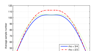
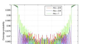

Refer to caption
Refer to caption
Figure 5: Double-parabolic sampling with various dilation coefficients

We have investigated the impact of confidence intervals on the performance of fully sequential sampling schemes constructed from the inclusion principle. We have observed that the stopping rule derived from Clopper-Pearson intervals generally outperforms the stopping rules derived from other types of confidence intervals. However, via appropriate choice of the dilation coefficient, the double-parabolic sampling scheme can perform uniformly better than the stopping rule derived from Clopper-Pearson intervals. To illustrate, consider the case that ε=0.1𝜀0.1\varepsilon=0.1 and δ=0.05𝛿0.05\delta=0.05. For stopping rules derived from Clopper-Pearson intervals, Fishman’s intervals, Wilson’s intervals, and revised Wald intervals with a=4𝑎4a=4, we have determined that to guarantee the prescribed confidence level 1δ=0.951𝛿0.951-\delta=0.95, it suffices to set the coverage tuning parameter ζ𝜁\zeta as 0.5, 1, 2.40.512.40.5,\;1,\;2.4 and 0.370.370.37, respectively. For the stopping rule derived from Wald intervals, we have determined ζ=0.77𝜁0.77\zeta=0.77 to ensure the confidence level, under the condition that the minimum sample size is taken as 1εln1ζδ1𝜀1𝜁𝛿\left\lceil\frac{1}{\varepsilon}\ln\frac{1}{\zeta\delta}\right\rceil. Recall that for the double-parabolic sampling scheme with ρ=34𝜌34\rho=\frac{3}{4}, we have obtained ζ=2.4𝜁2.4\zeta=2.4 for purpose of guaranteeing the confidence level. The average sample numbers of these sampling schemes are shown in Figure 6. From these plots, it can be seen that as compared to the stopping rule derived from Clopper-Pearson intervals, the stopping rule derived from the revised Wald intervals performs better in the region of p𝑝p close to 00 or 111, but performs worse in the region of p𝑝p in the middle of (0,1)01(0,1). The performance of stopping rules from Fishman’s intervals (i.e., from Chernoff bound) and Wald intervals are obviously inferior as compared to that of the stopping rule derived from Clopper-Pearson intervals. It can be observed that the double-parabolic sampling scheme uniformly outperforms the stopping rule derived from Clopper-Pearson intervals.
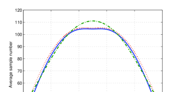
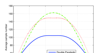

Refer to caption
Refer to caption
Figure 6: Comparison of average sample numbers

6.5 Estimation with High Confidence Level

In some situations, we need to estimate a binomial proportion with a high confidence level. For example, one might want to construct a sampling scheme such that, for ε=0.05𝜀0.05\varepsilon=0.05 and δ=1010𝛿superscript1010\delta=10^{-10}, the resultant sequential estimator 𝒑^^𝒑\widehat{\boldsymbol{p}} satisfies Pr{|𝒑^p|<εp}>1δPr^𝒑𝑝bra𝜀𝑝1𝛿\Pr\{|\widehat{\boldsymbol{p}}-p|<\varepsilon\mid p\}>1-\delta for any p(0,1)𝑝01p\in(0,1). By working with the complementary coverage probability, we determined that it suffices to let the dilation coefficient ρ=34𝜌34\rho=\frac{3}{4} and the coverage tuning parameter ζ=7.65𝜁7.65\zeta=7.65. The stopping boundary and the function of coverage probability with respect to the binomial proportion are displayed, respectively, in the left and right sides of Figure 7. As addressed in Section 5.3, it should be noted that it is impossible to obtain such a sampling scheme without working with the complementary coverage probability.
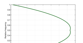
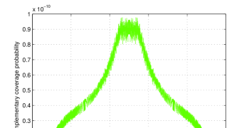

Refer to caption
Refer to caption
Figure 7: Double-parabolic sampling with ε=0.05,δ=1010,ρ=34formulae-sequence𝜀0.05formulae-sequence𝛿superscript1010𝜌34\varepsilon=0.05,\;\delta=10^{-10},\;\rho=\frac{3}{4} and ζ=7.65𝜁7.65\zeta=7.65

7 Illustrative Examples for Clinical Trials

In this section, we shall illustrate the applications of our double-parabolic group sequential estimation method in clinical trials.

An example of our double-parabolic sampling scheme can be illustrated as follows. Assume that ε=δ=0.05𝜀𝛿0.05\varepsilon=\delta=0.05 is given and that the sampling procedure is expected to have 777 stages with sample sizes satisfying (5). Choosing ρ=34𝜌34\rho=\frac{3}{4}, we have determined that it suffices to take ζ=2.6759𝜁2.6759\zeta=2.6759 to guarantee that the coverage probability is no less than 1δ=0.951𝛿0.951-\delta=0.95 for all p(0,1)𝑝01p\in(0,1). Accordingly, the sample sizes of this sampling scheme are calculated as 59,116,173,231,288,3455911617323128834559,116,173,231,288,345 and 403403403. This sampling scheme, with a sample path, is shown in the left side of Figure 8. In this case, the stopping rule can be equivalently described by virtue of Figure 8 as: Continue sampling until (𝒑^,n)subscript^𝒑subscript𝑛(\widehat{\boldsymbol{p}}_{\ell},n_{\ell}) hit a green line at some stage. The coverage probability is shown in the right side of Figure 8.

To apply this estimation method in a clinical trial for estimating the proportion p𝑝p of a binomial response with margin of error 0.050.050.05 and confidence level 95%percent9595\%, we can have seven groups of patients with group sizes 59,57,57,58,57,5759575758575759,57,57,58,57,57 and 585858. In the first stage, we conduct experiment with the 595959 patients of the first group. We observe the relative frequency of response and record it as 𝒑^1subscript^𝒑1\widehat{\boldsymbol{p}}_{1}. Suppose there are 121212 patients having positive responses, then the relative frequency at the first stage is 𝒑^1=1259=0.2034subscript^𝒑112590.2034\widehat{\boldsymbol{p}}_{1}=\frac{12}{59}=0.2034. With the values of (𝒑^1,n1)=(0.2034,59)subscript^𝒑1subscript𝑛10.203459(\widehat{\boldsymbol{p}}_{1},n_{1})=(0.2034,59), we check if the stopping rule is satisfied. This is equivalent to see if the point (𝒑^1,n1)subscript^𝒑1subscript𝑛1(\widehat{\boldsymbol{p}}_{1},n_{1}) hit a green line at the first stage. For such value of (𝒑^1,n1)subscript^𝒑1subscript𝑛1(\widehat{\boldsymbol{p}}_{1},n_{1}), it can be seen that the stopping condition is not fulfilled. So, we need to conduct the second stage of experiment with the 575757 patients of the second group. We observe the response of these 575757 patients. Suppose we observe that 555 patients among this group have positive responses. Then, we add 555 with 121212, the number of positive responses before the second stage, to obtain 171717 positive responses among n2=59+57=116subscript𝑛25957116n_{2}=59+57=116 patients. So, at the second stage, we get the relative frequency 𝒑^2=17116=0.1466subscript^𝒑2171160.1466\widehat{\boldsymbol{p}}_{2}=\frac{17}{116}=0.1466. Since the stopping rule is not satisfied with the values of (𝒑^2,n2)=(0.1466,116)subscript^𝒑2subscript𝑛20.1466116(\widehat{\boldsymbol{p}}_{2},n_{2})=(0.1466,116), we need to conduct the third stage of experiment with the 575757 patients of the third group. Suppose we observe that 141414 patients among this group have positive responses. Then, we add 141414 with 171717, the number of positive responses before the third stage, to get 313131 positive responses among n3=59+57+57=173subscript𝑛3595757173n_{3}=59+57+57=173 patients. So, at the third stage, we get the relative frequency 𝒑^3=31173=0.1792subscript^𝒑3311730.1792\widehat{\boldsymbol{p}}_{3}=\frac{31}{173}=0.1792. Since the stopping rule is not satisfied with the values of (𝒑^3,n3)=(0.1792,173)subscript^𝒑3subscript𝑛30.1792173(\widehat{\boldsymbol{p}}_{3},n_{3})=(0.1792,173), we need to conduct the fourth stage of experiment with the 585858 patients of the fourth group. Suppose we observe that 151515 patients among this group have positive responses. Then, we add 151515 with 313131, the number of positive responses before the fourth stage, to get 464646 positive responses among n4=59+57+57+58=231subscript𝑛459575758231n_{4}=59+57+57+58=231 patients. So, at the fourth stage, we get the relative frequency 𝒑^4=46231=0.1991subscript^𝒑4462310.1991\widehat{\boldsymbol{p}}_{4}=\frac{46}{231}=0.1991. Since the stopping rule is not satisfied with the values of (𝒑^4,n4)=(0.1991,231)subscript^𝒑4subscript𝑛40.1991231(\widehat{\boldsymbol{p}}_{4},n_{4})=(0.1991,231), we need to conduct the fifth stage of experiment with the 575757 patients of the fifth group. Suppose we observe that 666 patients among this group have positive responses. Then, we add 666 with 464646, the number of positive responses before the fifth stage, to get 525252 positive responses among n5=59+57+57+58+57=288subscript𝑛55957575857288n_{5}=59+57+57+58+57=288 patients. So, at the fifth stage, we get the relative frequency 𝒑^5=52288=0.1806subscript^𝒑5522880.1806\widehat{\boldsymbol{p}}_{5}=\frac{52}{288}=0.1806. It can be seen that the stopping rule is satisfied with the values of (𝒑^5,n5)=(0.1806,288)subscript^𝒑5subscript𝑛50.1806288(\widehat{\boldsymbol{p}}_{5},n_{5})=(0.1806,288). Therefore, we can terminate the sampling experiment and take 𝒑^=52288=0.1806^𝒑522880.1806\widehat{\boldsymbol{p}}=\frac{52}{288}=0.1806 as an estimate of the proportion of the whole population having positive responses. With a 95%percent9595\% confidence level, one can believe that the difference between the true value of p𝑝p and its estimate 𝒑^=0.1806^𝒑0.1806\widehat{\boldsymbol{p}}=0.1806 is less than 0.050.050.05.


Refer to caption
Refer to caption
Figure 8: Double-parabolic sampling with ε=δ=0.05,s=7,ρ=34formulae-sequence𝜀𝛿0.05formulae-sequence𝑠7𝜌34\varepsilon=\delta=0.05,s=7,\rho=\frac{3}{4} and ζ=2.6759𝜁2.6759\zeta=2.6759

In this experiment, we only use 288288288 samples to obtain the estimate for p𝑝p. Except the roundoff error, there is no other source of error for reporting statistical accuracy, since no asymptotic approximation is involved. As compared to fixed-sample-size procedure, we achieved a substantial save of samples. To see this, one can check that using the rigorous formula (24) gives a sample size 738738738, which is overly conservative. From the classical approximate formula (22), the sample size is determined as 385385385, which has been known to be insufficient to guarantee the prescribed confidence level 95%percent9595\%. The exact method of [16] shows that at least 391391391 samples are needed. As compared to the best fixed sample size obtained by the method of [16], the reduction of sample sizes resulted from our double-parabolic sampling scheme is 391288=103391288103391-288=103. It can be seen that the fixed-sample-size procedure wastes 103288=35.76%103288percent35.76\frac{103}{288}=35.76\% samples as compared to our group sequential method, which is also an exact method. This percentage may not be serious if it were a save of number of simulation runs. However, as the number count is for patients, the reduction of samples is important for ethical and economical reasons. Using our group sequential method, the worst-case sample size is equal to 403403403, which is only 121212 more than the minimum sample size of fixed-sample procedure. However, a lot of samples can be saved in the average case.

As ε𝜀\varepsilon or δ𝛿\delta become smaller, the reduction of samples is more significant. For example, let ε=0.02𝜀0.02\varepsilon=0.02 and δ=0.05𝛿0.05\delta=0.05, we have a double-parabolic sample scheme with 101010 stages. The sampling scheme, with a sample path, is shown in the left side of Figure 9. The coverage probability is shown in the right side of Figure 9.
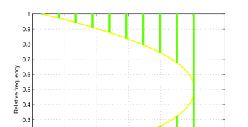
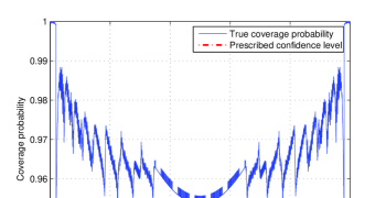

Refer to caption
Refer to caption
Figure 9: Double-parabolic sampling with ε=0.02,δ=0.05,s=10,ρ=34formulae-sequence𝜀0.02formulae-sequence𝛿0.05formulae-sequence𝑠10𝜌34\varepsilon=0.02,\;\delta=0.05,\;s=10,\;\rho=\frac{3}{4} and ζ=2.6725𝜁2.6725\zeta=2.6725

8 Conclusion

In this paper, we have reviewed recent development of group sequential estimation methods for a binomial proportion. We have illustrated the inclusion principle and its applications to various stopping rules. We have introduced computational techniques in the literature, which suffice for determining parameters of stopping rules to guarantee desired confidence levels. Moreover, we have proposed a new family of sampling schemes with stopping boundary of double-parabolic shape, which are parameterized by the coverage tuning parameter and the dilation coefficient. These parameters can be determined by the exact computational techniques to reduce the sampling cost, while ensuring prescribed confidence levels. The new family of sampling schemes are extremely simple in structure and asymptotically optimal as the margin of error tends to 00. We have established analytic bounds for the distribution and expectation of the sample number at the termination of the sampling process. We have obtained parameter values via the exact computational techniques for the proposed sampling schemes such that the confidence levels are guaranteed and that the sampling schemes are generally more efficient as compared to existing ones.

Appendix A Proof of Theorem 1

Consider function g(x,z)=(xz)2x(1x)𝑔𝑥𝑧superscript𝑥𝑧2𝑥1𝑥g(x,z)=\frac{(x-z)^{2}}{x(1-x)} for x(0,1)𝑥01x\in(0,1) and z[0,1]𝑧01z\in[0,1]. It can be checked that g(x,z)x=(xz)[z(1x)+x(1z)][x(1x)]2𝑔𝑥𝑧𝑥𝑥𝑧delimited-[]𝑧1𝑥𝑥1𝑧superscriptdelimited-[]𝑥1𝑥2\frac{\partial g(x,z)}{\partial x}=(x-z)[z(1-x)+x(1-z)][x(1-x)]^{-2}, which shows that for any fixed z[0,1]𝑧01z\in[0,1], g(x,z)𝑔𝑥𝑧-g(x,z) is a unimodal function of x(0,1)𝑥01x\in(0,1), with a maximum attained at x=z𝑥𝑧x=z. By such a property of g(x,z)𝑔𝑥𝑧g(x,z) and the definition of Wilson’s confidence intervals, we have

{𝒑^εL}={0<𝒑^εL}{𝒑^ε}={0<𝒑^εL𝒑^,g(L,𝒑^)=𝒵ζδ2n}{𝒑^ε}\displaystyle\left\{\widehat{\boldsymbol{p}}_{\ell}-\varepsilon\leq L_{\ell}\right\}=\left\{0<\widehat{\boldsymbol{p}}_{\ell}-\varepsilon\leq L_{\ell}\right\}\cup\{\widehat{\boldsymbol{p}}_{\ell}\leq\varepsilon\}=\left\{0<\widehat{\boldsymbol{p}}_{\ell}-\varepsilon\leq L_{\ell}\leq\widehat{\boldsymbol{p}}_{\ell},\;g(L_{\ell},\widehat{\boldsymbol{p}}_{\ell})=\frac{\mathcal{Z}_{\zeta\delta}^{2}}{n_{\ell}}\right\}\cup\{\widehat{\boldsymbol{p}}_{\ell}\leq\varepsilon\}
={𝒑^>ε,ε2(𝒑^ε)[1(𝒑^ε)]𝒵ζδ2n}{𝒑^ε}absentformulae-sequencesubscript^𝒑𝜀superscript𝜀2subscript^𝒑𝜀delimited-[]1subscript^𝒑𝜀superscriptsubscript𝒵𝜁𝛿2subscript𝑛subscript^𝒑𝜀\displaystyle=\left\{\widehat{\boldsymbol{p}}_{\ell}>\varepsilon,\;\frac{\varepsilon^{2}}{(\widehat{\boldsymbol{p}}_{\ell}-\varepsilon)[1-(\widehat{\boldsymbol{p}}_{\ell}-\varepsilon)]}\geq\frac{\mathcal{Z}_{\zeta\delta}^{2}}{n_{\ell}}\right\}\cup\{\widehat{\boldsymbol{p}}_{\ell}\leq\varepsilon\}\qquad\qquad\qquad\qquad\qquad\qquad\qquad\quad

and

{𝒑^+εU}={1>𝒑^+εU}{𝒑^+ε1}={1>𝒑^+εU𝒑^,g(U,𝒑^)=𝒵ζδ2n}\displaystyle\left\{\widehat{\boldsymbol{p}}_{\ell}+\varepsilon\geq U_{\ell}\right\}=\left\{1>\widehat{\boldsymbol{p}}_{\ell}+\varepsilon\geq U_{\ell}\right\}\cup\{\widehat{\boldsymbol{p}}_{\ell}+\varepsilon\geq 1\}=\left\{1>\widehat{\boldsymbol{p}}_{\ell}+\varepsilon\geq U_{\ell}\geq\widehat{\boldsymbol{p}}_{\ell},\;g(U_{\ell},\widehat{\boldsymbol{p}}_{\ell})=\frac{\mathcal{Z}_{\zeta\delta}^{2}}{n_{\ell}}\right\}
{𝒑^+ε1}={𝒑^<1ε,ε2(𝒑^+ε)[1(𝒑^+ε)]𝒵ζδ2n}{𝒑^1ε}subscript^𝒑𝜀1formulae-sequencesubscript^𝒑1𝜀superscript𝜀2subscript^𝒑𝜀delimited-[]1subscript^𝒑𝜀superscriptsubscript𝒵𝜁𝛿2subscript𝑛subscript^𝒑1𝜀\displaystyle\cup\{\widehat{\boldsymbol{p}}_{\ell}+\varepsilon\geq 1\}=\left\{\widehat{\boldsymbol{p}}_{\ell}<1-\varepsilon,\;\frac{\varepsilon^{2}}{(\widehat{\boldsymbol{p}}_{\ell}+\varepsilon)[1-(\widehat{\boldsymbol{p}}_{\ell}+\varepsilon)]}\geq\frac{\mathcal{Z}_{\zeta\delta}^{2}}{n_{\ell}}\right\}\cup\{\widehat{\boldsymbol{p}}_{\ell}\geq 1-\varepsilon\}

for =1,,s1𝑠\ell=1,\cdots,s, where we have used the fact that {𝒑^>ε}{L>0},{𝒑^<1ε}{U<1}formulae-sequencesubscript^𝒑𝜀subscript𝐿0subscript^𝒑1𝜀subscript𝑈1\{\widehat{\boldsymbol{p}}_{\ell}>\varepsilon\}\subseteq\{L_{\ell}>0\},\;\{\widehat{\boldsymbol{p}}_{\ell}<1-\varepsilon\}\subseteq\{U_{\ell}<1\} and 0L𝒑^U10subscript𝐿subscript^𝒑subscript𝑈10\leq L_{\ell}\leq\widehat{\boldsymbol{p}}_{\ell}\leq U_{\ell}\leq 1. Recall that 0<ε<120𝜀120<\varepsilon<\frac{1}{2}. It follows that

{𝒑^εLU𝒑^+ε}subscript^𝒑𝜀subscript𝐿subscript𝑈subscript^𝒑𝜀\displaystyle\left\{\widehat{\boldsymbol{p}}_{\ell}-\varepsilon\leq L_{\ell}\leq U_{\ell}\leq\widehat{\boldsymbol{p}}_{\ell}+\varepsilon\right\}
={ε<𝒑^<1ε,ε2(𝒑^ε)[1(𝒑^ε)]𝒵ζδ2n,ε2(𝒑^+ε)[1(𝒑^+ε)]𝒵ζδ2n}\displaystyle=\left\{\varepsilon<\widehat{\boldsymbol{p}}_{\ell}<1-\varepsilon,\;\frac{\varepsilon^{2}}{(\widehat{\boldsymbol{p}}_{\ell}-\varepsilon)[1-(\widehat{\boldsymbol{p}}_{\ell}-\varepsilon)]}\geq\frac{\mathcal{Z}_{\zeta\delta}^{2}}{n_{\ell}},\;\frac{\varepsilon^{2}}{(\widehat{\boldsymbol{p}}_{\ell}+\varepsilon)[1-(\widehat{\boldsymbol{p}}_{\ell}+\varepsilon)]}\geq\frac{\mathcal{Z}_{\zeta\delta}^{2}}{n_{\ell}}\right\}
{𝒑^ε,ε2(𝒑^+ε)[1(𝒑^+ε)]𝒵ζδ2n}{𝒑^1ε,ε2(𝒑^ε)[1(𝒑^ε)]𝒵ζδ2n}formulae-sequencesubscript^𝒑𝜀superscript𝜀2subscript^𝒑𝜀delimited-[]1subscript^𝒑𝜀superscriptsubscript𝒵𝜁𝛿2subscript𝑛formulae-sequencesubscript^𝒑1𝜀superscript𝜀2subscript^𝒑𝜀delimited-[]1subscript^𝒑𝜀superscriptsubscript𝒵𝜁𝛿2subscript𝑛\displaystyle\bigcup\left\{\widehat{\boldsymbol{p}}_{\ell}\leq\varepsilon,\;\frac{\varepsilon^{2}}{(\widehat{\boldsymbol{p}}_{\ell}+\varepsilon)[1-(\widehat{\boldsymbol{p}}_{\ell}+\varepsilon)]}\geq\frac{\mathcal{Z}_{\zeta\delta}^{2}}{n_{\ell}}\right\}\bigcup\left\{\widehat{\boldsymbol{p}}_{\ell}\geq 1-\varepsilon,\;\frac{\varepsilon^{2}}{(\widehat{\boldsymbol{p}}_{\ell}-\varepsilon)[1-(\widehat{\boldsymbol{p}}_{\ell}-\varepsilon)]}\geq\frac{\mathcal{Z}_{\zeta\delta}^{2}}{n_{\ell}}\right\}
={ε<𝒑^<1ε,(|𝒑^12|ε)214n(ε𝒵ζδ)2}\displaystyle=\left\{\varepsilon<\widehat{\boldsymbol{p}}_{\ell}<1-\varepsilon,\;\left(\left|\widehat{\boldsymbol{p}}_{\ell}-\frac{1}{2}\right|-\varepsilon\right)^{2}\geq\frac{1}{4}-n_{\ell}\left(\frac{\varepsilon}{\mathcal{Z}_{\zeta\delta}}\right)^{2}\right\}\bigcup
{𝒑^ε,(|𝒑^12|ε)214n(ε𝒵ζδ)2}{𝒑^1ε,(|𝒑^12|ε)214n(ε𝒵ζδ)2}formulae-sequencesubscript^𝒑𝜀superscriptsubscript^𝒑12𝜀214subscript𝑛superscript𝜀subscript𝒵𝜁𝛿2formulae-sequencesubscript^𝒑1𝜀superscriptsubscript^𝒑12𝜀214subscript𝑛superscript𝜀subscript𝒵𝜁𝛿2\displaystyle\left\{\widehat{\boldsymbol{p}}_{\ell}\leq\varepsilon,\;\left(\left|\widehat{\boldsymbol{p}}_{\ell}-\frac{1}{2}\right|-\varepsilon\right)^{2}\geq\frac{1}{4}-n_{\ell}\left(\frac{\varepsilon}{\mathcal{Z}_{\zeta\delta}}\right)^{2}\right\}\bigcup\left\{\widehat{\boldsymbol{p}}_{\ell}\geq 1-\varepsilon,\;\left(\left|\widehat{\boldsymbol{p}}_{\ell}-\frac{1}{2}\right|-\varepsilon\right)^{2}\geq\frac{1}{4}-n_{\ell}\left(\frac{\varepsilon}{\mathcal{Z}_{\zeta\delta}}\right)^{2}\right\}
={(|𝒑^12|ε)214n(ε𝒵ζδ)2}absentsuperscriptsubscript^𝒑12𝜀214subscript𝑛superscript𝜀subscript𝒵𝜁𝛿2\displaystyle=\left\{\left(\left|\widehat{\boldsymbol{p}}_{\ell}-\frac{1}{2}\right|-\varepsilon\right)^{2}\geq\frac{1}{4}-n_{\ell}\left(\frac{\varepsilon}{\mathcal{Z}_{\zeta\delta}}\right)^{2}\right\}

for =1,,s1𝑠\ell=1,\cdots,s. This completes the proof of the theorem.

Appendix B Proof of Theorem 2

By the assumption that ns12ε2ln1ζδsubscript𝑛𝑠12superscript𝜀21𝜁𝛿n_{s}\geq\frac{1}{2\varepsilon^{2}}\ln\frac{1}{\zeta\delta}, we have 14+ε2ns2ln(ζδ)014superscript𝜀2subscript𝑛𝑠2𝜁𝛿0\frac{1}{4}+\frac{\varepsilon^{2}n_{s}}{2\ln(\zeta\delta)}\leq 0 and consequently, Pr{(|𝒑^s12|ρε)214+ε2ns2ln(ζδ)}=1Prsuperscriptsubscript^𝒑𝑠12𝜌𝜀214superscript𝜀2subscript𝑛𝑠2𝜁𝛿1\Pr\{(|\widehat{\boldsymbol{p}}_{s}-\frac{1}{2}|-\rho\varepsilon)^{2}\geq\frac{1}{4}+\frac{\varepsilon^{2}n_{s}}{2\ln(\zeta\delta)}\}=1. It follows from the definition of the sampling scheme that the sampling process must stop at or before the s𝑠s-th stage. In other words, Pr{𝒍s}=1Pr𝒍𝑠1\Pr\{\boldsymbol{l}\leq s\}=1. This allows one to write

Pr{|𝒑^p|εp}Pr^𝒑𝑝conditional𝜀𝑝\displaystyle\Pr\{|\widehat{\boldsymbol{p}}-p|\geq\varepsilon\mid p\} =\displaystyle= =1sPr{|𝒑^p|ε,𝒍=p}==1sPr{|𝒑^p|ε,𝒍=p}superscriptsubscript1𝑠Pr^𝒑𝑝𝜀𝒍conditional𝑝superscriptsubscript1𝑠Prsubscript^𝒑𝑝𝜀𝒍conditional𝑝\displaystyle\sum_{\ell=1}^{s}\Pr\{|\widehat{\boldsymbol{p}}-p|\geq\varepsilon,\;\boldsymbol{l}=\ell\mid p\}=\sum_{\ell=1}^{s}\Pr\{|\widehat{\boldsymbol{p}}_{\ell}-p|\geq\varepsilon,\;\boldsymbol{l}=\ell\mid p\} (25)
\displaystyle\leq =1sPr{|𝒑^p|εp}superscriptsubscript1𝑠Prsubscript^𝒑𝑝conditional𝜀𝑝\displaystyle\sum_{\ell=1}^{s}\Pr\{|\widehat{\boldsymbol{p}}_{\ell}-p|\geq\varepsilon\mid p\}

for p(0,1)𝑝01p\in(0,1). By virtue of the well-known Chernoff-Hoeffding bound [3, 26], we have

Pr{|𝒑^p|εp}2exp(2nε2)Prsubscript^𝒑𝑝conditional𝜀𝑝22subscript𝑛superscript𝜀2\Pr\{|\widehat{\boldsymbol{p}}_{\ell}-p|\geq\varepsilon\mid p\}\leq 2\exp(-2n_{\ell}\varepsilon^{2}) (26)

for =1,,s1𝑠\ell=1,\cdots,s. Making use of (25), (26) and the fact that n12ρ(1ερ)ln1ζδsubscript𝑛12𝜌1𝜀𝜌1𝜁𝛿n_{1}\geq 2\rho(\frac{1}{\varepsilon}-\rho)\ln\frac{1}{\zeta\delta} as can be seen from (18), we have

Pr{|𝒑^p|εp}Pr^𝒑𝑝conditional𝜀𝑝\displaystyle\Pr\{|\widehat{\boldsymbol{p}}-p|\geq\varepsilon\mid p\} \displaystyle\leq 2=1sexp(2nε2)2m=n1exp(2mε2)=2exp(2n1ε2)1exp(2ε2)2superscriptsubscript1𝑠2subscript𝑛superscript𝜀22superscriptsubscript𝑚subscript𝑛12𝑚superscript𝜀222subscript𝑛1superscript𝜀212superscript𝜀2\displaystyle 2\sum_{\ell=1}^{s}\exp(-2n_{\ell}\varepsilon^{2})\leq 2\sum_{m=n_{1}}^{\infty}\exp(-2m\varepsilon^{2})=\frac{2\exp(-2n_{1}\varepsilon^{2})}{1-\exp(-2\varepsilon^{2})}
\displaystyle\leq 2exp(2ε2×2ρ(1ερ)ln1ζδ)1exp(2ε2)=2exp(4ερ(1ρε)ln(ζδ))1exp(2ε2)22superscript𝜀22𝜌1𝜀𝜌1𝜁𝛿12superscript𝜀224𝜀𝜌1𝜌𝜀𝜁𝛿12superscript𝜀2\displaystyle\frac{2\exp\left(-2\varepsilon^{2}\times 2\rho(\frac{1}{\varepsilon}-\rho)\ln\frac{1}{\zeta\delta}\right)}{1-\exp(-2\varepsilon^{2})}=\frac{2\exp\left(4\varepsilon\rho(1-\rho\varepsilon)\ln(\zeta\delta)\right)}{1-\exp(-2\varepsilon^{2})}

for any p(0,1)𝑝01p\in(0,1). Therefore, to guarantee that Pr{|𝒑^p|<εp}1δPr^𝒑𝑝bra𝜀𝑝1𝛿\Pr\{|\widehat{\boldsymbol{p}}-p|<\varepsilon\mid p\}\geq 1-\delta for any p(0,1)𝑝01p\in(0,1), it is sufficient to choose ζ𝜁\zeta such that 2exp(4ερ(1ρε)ln(ζδ))δ[1exp(2ε2)]24𝜀𝜌1𝜌𝜀𝜁𝛿𝛿delimited-[]12superscript𝜀22\exp\left(4\varepsilon\rho(1-\rho\varepsilon)\ln(\zeta\delta)\right)\leq\delta[1-\exp(-2\varepsilon^{2})]. This inequality can be written as 4ερ(1ρε)ln(ζδ)lnδ2+ln[1exp(2ε2)]4𝜀𝜌1𝜌𝜀𝜁𝛿𝛿212superscript𝜀24\varepsilon\rho(1-\rho\varepsilon)\ln(\zeta\delta)\leq\ln\frac{\delta}{2}+\ln\left[1-\exp(-2\varepsilon^{2})\right] or equivalently, ζ1δexp(lnδ2+ln[1exp(2ε2)]4ερ(1ρε))𝜁1𝛿𝛿212superscript𝜀24𝜀𝜌1𝜌𝜀\zeta\leq\frac{1}{\delta}\exp\left(\frac{\ln\frac{\delta}{2}+\ln\left[1-\exp(-2\varepsilon^{2})\right]}{4\varepsilon\rho(1-\rho\varepsilon)}\right). The proof of the theorem is thus completed.

Appendix C Proof of Theorem 3

First, we need to show that Pr{limε0𝐧N(p,ε,δ,ζ)=1p}=1Prsubscript𝜀0𝐧𝑁𝑝𝜀𝛿𝜁conditional1𝑝1\Pr\{\lim_{\varepsilon\to 0}\frac{\mathbf{n}}{N(p,\varepsilon,\delta,\zeta)}=1\mid p\}=1 for any p(0,1)𝑝01p\in(0,1). Clearly, the sample number 𝐧𝐧\mathbf{n} is a random number dependent on ε𝜀\varepsilon. Note that for any ωΩ𝜔Ω\omega\in\Omega, the sequences {X¯𝐧(ω)(ω)}ε(0,1)subscriptsubscript¯𝑋𝐧𝜔𝜔𝜀01\{\overline{X}_{\mathbf{n}(\omega)}(\omega)\}_{\varepsilon\in(0,1)} and {X¯𝐧(ω)1(ω)}ε(0,1)subscriptsubscript¯𝑋𝐧𝜔1𝜔𝜀01\{\overline{X}_{\mathbf{n}(\omega)-1}(\omega)\}_{\varepsilon\in(0,1)} are subsets of {X¯m(ω)}m=1superscriptsubscriptsubscript¯𝑋𝑚𝜔𝑚1\{\overline{X}_{m}(\omega)\}_{m=1}^{\infty}. By the strong law of large numbers, for almost every ωΩ𝜔Ω\omega\in\Omega, the sequence {X¯m(ω)}m=1superscriptsubscriptsubscript¯𝑋𝑚𝜔𝑚1\{\overline{X}_{m}(\omega)\}_{m=1}^{\infty} converges to p𝑝p. Since every subsequence of a convergent sequence must converge, it follows that the sequences {X¯𝐧(ω)(ω)}ε(0,1)subscriptsubscript¯𝑋𝐧𝜔𝜔𝜀01\{\overline{X}_{\mathbf{n}(\omega)}(\omega)\}_{\varepsilon\in(0,1)} and {X¯𝐧(ω)1(ω)}ε(0,1)subscriptsubscript¯𝑋𝐧𝜔1𝜔𝜀01\{\overline{X}_{\mathbf{n}(\omega)-1}(\omega)\}_{\varepsilon\in(0,1)} converge to p𝑝p as ε0𝜀0\varepsilon\to 0 provided that 𝐧(ω)𝐧𝜔\mathbf{n}(\omega)\to\infty as ε0𝜀0\varepsilon\to 0. Since it is certain that 𝐧2ρ(1ερ)ln1ζδ𝐧2𝜌1𝜀𝜌1𝜁𝛿\mathbf{n}\geq 2\rho(\frac{1}{\varepsilon}-\rho)\ln\frac{1}{\zeta\delta}\to\infty as ε0𝜀0\varepsilon\to 0, we have that {limε0𝐧1𝐧=1}subscript𝜀0𝐧1𝐧1\left\{\lim_{\varepsilon\to 0}\frac{\mathbf{n}-1}{\mathbf{n}}=1\right\} is a sure event. It follows that B={limε0X¯𝐧1=p,limε0X¯𝐧=p,limε0𝐧1𝐧=1}𝐵formulae-sequencesubscript𝜀0subscript¯𝑋𝐧1𝑝formulae-sequencesubscript𝜀0subscript¯𝑋𝐧𝑝subscript𝜀0𝐧1𝐧1B=\{\lim_{\varepsilon\to 0}\overline{X}_{\mathbf{n}-1}=p,\;\lim_{\varepsilon\to 0}\overline{X}_{\mathbf{n}}=p,\;\lim_{\varepsilon\to 0}\frac{\mathbf{n}-1}{\mathbf{n}}=1\} is an almost sure event. By the definition of the sampling scheme, we have that

A={(|X¯𝐧112|ρε)2<14+ε2(𝐧1)2ln(ζδ),(|X¯𝐧12|ρε)214+ε2𝐧2ln(ζδ)}𝐴formulae-sequencesuperscriptsubscript¯𝑋𝐧112𝜌𝜀214superscript𝜀2𝐧12𝜁𝛿superscriptsubscript¯𝑋𝐧12𝜌𝜀214superscript𝜀2𝐧2𝜁𝛿A=\left\{\left(\left|\overline{X}_{\mathbf{n}-1}-\frac{1}{2}\right|-\rho\varepsilon\right)^{2}<\frac{1}{4}+\frac{\varepsilon^{2}(\mathbf{n}-1)}{2\ln(\zeta\delta)},\quad\left(\left|\overline{X}_{\mathbf{n}}-\frac{1}{2}\right|-\rho\varepsilon\right)^{2}\geq\frac{1}{4}+\frac{\varepsilon^{2}\mathbf{n}}{2\ln(\zeta\delta)}\right\}

is a sure event. Hence, AB𝐴𝐵A\cap B is an almost sure event. Define C={limε0𝐧N(p,ε,δ,ζ)=1}𝐶subscript𝜀0𝐧𝑁𝑝𝜀𝛿𝜁1C=\left\{\lim_{\varepsilon\to 0}\frac{\mathbf{n}}{N(p,\varepsilon,\delta,\zeta)}=1\right\}. We need to show that C𝐶C is an almost sure event. For this purpose, we let ωAB𝜔𝐴𝐵\omega\in A\cap B and expect to show that ωC𝜔𝐶\omega\in C. As a consequence of ωAB𝜔𝐴𝐵\omega\in A\cap B,

𝐧(ω)N(p,ε,δ,ζ)<𝐧(ω)𝐧(ω)1[14(|X¯𝐧(ω)1(ω)12|ρε)2]p(1p),limε0X¯𝐧(ω)1(ω)=p,limε0𝐧(ω)1𝐧(ω)=1.formulae-sequence𝐧𝜔𝑁𝑝𝜀𝛿𝜁𝐧𝜔𝐧𝜔1delimited-[]14superscriptsubscript¯𝑋𝐧𝜔1𝜔12𝜌𝜀2𝑝1𝑝formulae-sequencesubscript𝜀0subscript¯𝑋𝐧𝜔1𝜔𝑝subscript𝜀0𝐧𝜔1𝐧𝜔1\frac{\mathbf{n}(\omega)}{N(p,\varepsilon,\delta,\zeta)}<\frac{\mathbf{n}(\omega)}{\mathbf{n}(\omega)-1}\frac{\left[\frac{1}{4}-\left(\left|\overline{X}_{\mathbf{n}(\omega)-1}(\omega)-\frac{1}{2}\right|-\rho\varepsilon\right)^{2}\right]}{p(1-p)},\quad\lim_{\varepsilon\to 0}\overline{X}_{\mathbf{n}(\omega)-1}(\omega)=p,\quad\lim_{\varepsilon\to 0}\frac{\mathbf{n}(\omega)-1}{\mathbf{n}(\omega)}=1.

By the continuity of the function |x12|ρε𝑥12𝜌𝜀\left|x-\frac{1}{2}\right|-\rho\varepsilon with respect to x𝑥x and ε𝜀\varepsilon, we have

lim supε0𝐧(ω)N(p,ε,δ,ζ)limε0𝐧(ω)𝐧(ω)1×[14(|limε0X¯𝐧(ω)1(ω)12|limε0ρε)2]p(1p)=1.subscriptlimit-supremum𝜀0𝐧𝜔𝑁𝑝𝜀𝛿𝜁subscript𝜀0𝐧𝜔𝐧𝜔1delimited-[]14superscriptsubscript𝜀0subscript¯𝑋𝐧𝜔1𝜔12subscript𝜀0𝜌𝜀2𝑝1𝑝1\limsup_{\varepsilon\to 0}\frac{\mathbf{n}(\omega)}{N(p,\varepsilon,\delta,\zeta)}\leq\lim_{\varepsilon\to 0}\frac{\mathbf{n}(\omega)}{\mathbf{n}(\omega)-1}\times\frac{\left[\frac{1}{4}-\left(\left|\lim_{\varepsilon\to 0}\overline{X}_{\mathbf{n}(\omega)-1}(\omega)-\frac{1}{2}\right|-\lim_{\varepsilon\to 0}\rho\varepsilon\right)^{2}\right]}{p(1-p)}=1.\qquad (27)

On the other hand, as a consequence of ωAB𝜔𝐴𝐵\omega\in A\cap B,

𝐧(ω)N(p,ε,δ,ζ)[14(|X¯𝐧(ω)(ω)12|ρε)2]p(1p),limε0X¯𝐧(ω)(ω)=p.formulae-sequence𝐧𝜔𝑁𝑝𝜀𝛿𝜁delimited-[]14superscriptsubscript¯𝑋𝐧𝜔𝜔12𝜌𝜀2𝑝1𝑝subscript𝜀0subscript¯𝑋𝐧𝜔𝜔𝑝\frac{\mathbf{n}(\omega)}{N(p,\varepsilon,\delta,\zeta)}\geq\frac{\left[\frac{1}{4}-\left(\left|\overline{X}_{\mathbf{n}(\omega)}(\omega)-\frac{1}{2}\right|-\rho\varepsilon\right)^{2}\right]}{p(1-p)},\qquad\qquad\lim_{\varepsilon\to 0}\overline{X}_{\mathbf{n}(\omega)}(\omega)=p.

Making use of the continuity of the function |x12|ρε𝑥12𝜌𝜀\left|x-\frac{1}{2}\right|-\rho\varepsilon with respect to x𝑥x and ε𝜀\varepsilon, we have

lim infε0𝐧(ω)N(p,ε,δ,ζ)[14(|limε0X¯𝐧(ω)(ω)12|limε0ρε)2]p(1p)=1.subscriptlimit-infimum𝜀0𝐧𝜔𝑁𝑝𝜀𝛿𝜁delimited-[]14superscriptsubscript𝜀0subscript¯𝑋𝐧𝜔𝜔12subscript𝜀0𝜌𝜀2𝑝1𝑝1\liminf_{\varepsilon\to 0}\frac{\mathbf{n}(\omega)}{N(p,\varepsilon,\delta,\zeta)}\geq\frac{\left[\frac{1}{4}-\left(\left|\lim_{\varepsilon\to 0}\overline{X}_{\mathbf{n}(\omega)}(\omega)-\frac{1}{2}\right|-\lim_{\varepsilon\to 0}\rho\varepsilon\right)^{2}\right]}{p(1-p)}=1. (28)

Combining (27) and (28) yields limε0𝐧(ω)N(p,ε,δ,ζ)=1subscript𝜀0𝐧𝜔𝑁𝑝𝜀𝛿𝜁1\lim_{\varepsilon\to 0}\frac{\mathbf{n}(\omega)}{N(p,\varepsilon,\delta,\zeta)}=1 and thus ABC𝐴𝐵𝐶A\cap B\subseteq C. This implies that C𝐶C is an almost sure event and thus Pr{limε0𝐧N(p,ε,δ,ζ)=1p}=1Prsubscript𝜀0𝐧𝑁𝑝𝜀𝛿𝜁conditional1𝑝1\Pr\left\{\lim_{\varepsilon\to 0}\frac{\mathbf{n}}{N(p,\varepsilon,\delta,\zeta)}=1\mid p\right\}=1 for p(0,1)𝑝01p\in(0,1).

Next, we need to show that limε0Pr{|𝒑^p|<εp}=2Φ(2ln1ζδ)1subscript𝜀0Pr^𝒑𝑝bra𝜀𝑝2Φ21𝜁𝛿1\lim_{\varepsilon\to 0}\Pr\{|\widehat{\boldsymbol{p}}-p|<\varepsilon\mid p\}=2\Phi\left(\sqrt{2\ln\frac{1}{\zeta\delta}}\right)-1 for any p(0,1)𝑝01p\in(0,1). For simplicity of notations, let σ=p(1p)𝜎𝑝1𝑝\sigma=\sqrt{p(1-p)} and a=2ln1ζδ𝑎21𝜁𝛿a=\sqrt{2\ln\frac{1}{\zeta\delta}}. Note that Pr{|𝒑^p|<εp}=Pr{|X¯𝐧p|<εp}=Pr{𝐧|X¯𝐧p|/σ<ε𝐧/σ}Pr^𝒑𝑝bra𝜀𝑝Prsubscript¯𝑋𝐧𝑝bra𝜀𝑝Pr𝐧subscript¯𝑋𝐧𝑝𝜎𝜀𝐧𝜎\Pr\{|\widehat{\boldsymbol{p}}-p|<\varepsilon\mid p\}=\Pr\{|\overline{X}_{\mathbf{n}}-p|<\varepsilon\mid p\}=\Pr\{\sqrt{\mathbf{n}}|\overline{X}_{\mathbf{n}}-p|/\sigma<\varepsilon\sqrt{\mathbf{n}}/\sigma\}. Clearly, for any η(0,a)𝜂0𝑎\eta\in(0,a),

Pr{𝐧|X¯𝐧p|/σ<ε𝐧/σ}Pr𝐧subscript¯𝑋𝐧𝑝𝜎𝜀𝐧𝜎\displaystyle\Pr\{\sqrt{\mathbf{n}}|\overline{X}_{\mathbf{n}}-p|/\sigma<\varepsilon\sqrt{\mathbf{n}}/\sigma\} \displaystyle\leq Pr{𝐧|X¯𝐧p|/σ<ε𝐧/σ,ε𝐧/σ[aη,a+η]}Pr𝐧subscript¯𝑋𝐧𝑝𝜎𝜀𝐧𝜎𝜀𝐧𝜎𝑎𝜂𝑎𝜂\displaystyle\Pr\{\sqrt{\mathbf{n}}|\overline{X}_{\mathbf{n}}-p|/\sigma<\varepsilon\sqrt{\mathbf{n}}/\sigma,\;\varepsilon\sqrt{\mathbf{n}}/\sigma\in[a-\eta,a+\eta]\} (29)
+Pr{ε𝐧/σ[aη,a+η]}Pr𝜀𝐧𝜎𝑎𝜂𝑎𝜂\displaystyle+\Pr\{\varepsilon\sqrt{\mathbf{n}}/\sigma\notin[a-\eta,a+\eta]\}
\displaystyle\leq Pr{𝐧|X¯𝐧p|/σ<a+η,ε𝐧/σ[aη,a+η]}Pr𝐧subscript¯𝑋𝐧𝑝𝜎𝑎𝜂𝜀𝐧𝜎𝑎𝜂𝑎𝜂\displaystyle\Pr\{\sqrt{\mathbf{n}}|\overline{X}_{\mathbf{n}}-p|/\sigma<a+\eta,\;\varepsilon\sqrt{\mathbf{n}}/\sigma\in[a-\eta,a+\eta]\}
+Pr{ε𝐧/σ[aη,a+η]}Pr𝜀𝐧𝜎𝑎𝜂𝑎𝜂\displaystyle+\Pr\{\varepsilon\sqrt{\mathbf{n}}/\sigma\notin[a-\eta,a+\eta]\}
\displaystyle\leq Pr{𝐧|X¯𝐧p|/σ<a+η}+Pr{ε𝐧/σ[aη,a+η]}Pr𝐧subscript¯𝑋𝐧𝑝𝜎𝑎𝜂Pr𝜀𝐧𝜎𝑎𝜂𝑎𝜂\displaystyle\Pr\{\sqrt{\mathbf{n}}|\overline{X}_{\mathbf{n}}-p|/\sigma<a+\eta\}+\Pr\{\varepsilon\sqrt{\mathbf{n}}/\sigma\notin[a-\eta,a+\eta]\}\qquad\qquad

and

Pr{𝐧|X¯𝐧p|/σ<ε𝐧/σ}Pr{𝐧|X¯𝐧p|/σ<ε𝐧/σ,ε𝐧/σ[aη,a+η]}Pr𝐧subscript¯𝑋𝐧𝑝𝜎𝜀𝐧𝜎Pr𝐧subscript¯𝑋𝐧𝑝𝜎𝜀𝐧𝜎𝜀𝐧𝜎𝑎𝜂𝑎𝜂\displaystyle\Pr\{\sqrt{\mathbf{n}}|\overline{X}_{\mathbf{n}}-p|/\sigma<\varepsilon\sqrt{\mathbf{n}}/\sigma\}\geq\Pr\{\sqrt{\mathbf{n}}|\overline{X}_{\mathbf{n}}-p|/\sigma<\varepsilon\sqrt{\mathbf{n}}/\sigma,\;\varepsilon\sqrt{\mathbf{n}}/\sigma\in[a-\eta,a+\eta]\}
Pr{𝐧|X¯𝐧p|/σ<aη,ε𝐧/σ[aη,a+η]}absentPr𝐧subscript¯𝑋𝐧𝑝𝜎𝑎𝜂𝜀𝐧𝜎𝑎𝜂𝑎𝜂\displaystyle\geq\Pr\{\sqrt{\mathbf{n}}|\overline{X}_{\mathbf{n}}-p|/\sigma<a-\eta,\;\varepsilon\sqrt{\mathbf{n}}/\sigma\in[a-\eta,a+\eta]\}
Pr{𝐧|X¯𝐧p|/σ<aη}Pr{ε𝐧/σ[aη,a+η]}.absentPr𝐧subscript¯𝑋𝐧𝑝𝜎𝑎𝜂Pr𝜀𝐧𝜎𝑎𝜂𝑎𝜂\displaystyle\geq\Pr\{\sqrt{\mathbf{n}}|\overline{X}_{\mathbf{n}}-p|/\sigma<a-\eta\}-\Pr\{\varepsilon\sqrt{\mathbf{n}}/\sigma\notin[a-\eta,a+\eta]\}. (30)

Recall that we have established that 𝐧/N(p,ε,δ,ζ)1𝐧𝑁𝑝𝜀𝛿𝜁1\mathbf{n}/N(p,\varepsilon,\delta,\zeta)\to 1 almost surely as ε0𝜀0\varepsilon\to 0. This implies that ε𝐧/σa𝜀𝐧𝜎𝑎\varepsilon\sqrt{\mathbf{n}}/\sigma\to a and 𝐧/N(p,ε,δ,ζ)1𝐧𝑁𝑝𝜀𝛿𝜁1\mathbf{n}/N(p,\varepsilon,\delta,\zeta)\to 1 in probability as ε𝜀\varepsilon tends to zero. It follows from Anscombe’s random central limit theorem [2] that as ε𝜀\varepsilon tends to zero, 𝐧(X¯𝐧p)/σ𝐧subscript¯𝑋𝐧𝑝𝜎\sqrt{\mathbf{n}}(\overline{X}_{\mathbf{n}}-p)/\sigma converges in distribution to a Gaussian random variable with zero mean and unit variance. Hence, from (29),

lim supε0Pr{𝐧|X¯𝐧p|/σ<ε𝐧/σ}subscriptlimit-supremum𝜀0Pr𝐧subscript¯𝑋𝐧𝑝𝜎𝜀𝐧𝜎\displaystyle\limsup_{\varepsilon\to 0}\Pr\{\sqrt{\mathbf{n}}|\overline{X}_{\mathbf{n}}-p|/\sigma<\varepsilon\sqrt{\mathbf{n}}/\sigma\}
limε0Pr{𝐧|X¯𝐧p|/σ<a+η}+limε0Pr{ε𝐧/σ[aη,a+η]}=2Φ(a+η)1absentsubscript𝜀0Pr𝐧subscript¯𝑋𝐧𝑝𝜎𝑎𝜂subscript𝜀0Pr𝜀𝐧𝜎𝑎𝜂𝑎𝜂2Φ𝑎𝜂1\displaystyle\leq\lim_{\varepsilon\to 0}\Pr\{\sqrt{\mathbf{n}}|\overline{X}_{\mathbf{n}}-p|/\sigma<a+\eta\}+\lim_{\varepsilon\to 0}\Pr\{\varepsilon\sqrt{\mathbf{n}}/\sigma\notin[a-\eta,a+\eta]\}=2\Phi(a+\eta)-1

and from (30),

lim infε0Pr{𝐧|X¯𝐧p|/σ<ε𝐧/σ}subscriptlimit-infimum𝜀0Pr𝐧subscript¯𝑋𝐧𝑝𝜎𝜀𝐧𝜎\displaystyle\liminf_{\varepsilon\to 0}\Pr\{\sqrt{\mathbf{n}}|\overline{X}_{\mathbf{n}}-p|/\sigma<\varepsilon\sqrt{\mathbf{n}}/\sigma\}
limε0Pr{𝐧|X¯𝐧p|/σ<aη}limε0Pr{ε𝐧/σ[aη,a+η]}=2Φ(aη)1.absentsubscript𝜀0Pr𝐧subscript¯𝑋𝐧𝑝𝜎𝑎𝜂subscript𝜀0Pr𝜀𝐧𝜎𝑎𝜂𝑎𝜂2Φ𝑎𝜂1\displaystyle\geq\lim_{\varepsilon\to 0}\Pr\{\sqrt{\mathbf{n}}|\overline{X}_{\mathbf{n}}-p|/\sigma<a-\eta\}-\lim_{\varepsilon\to 0}\Pr\{\varepsilon\sqrt{\mathbf{n}}/\sigma\notin[a-\eta,a+\eta]\}=2\Phi(a-\eta)-1.

Since this argument holds for arbitrarily small η(0,a)𝜂0𝑎\eta\in(0,a), it must be true that

lim infε0Pr{𝐧|X¯𝐧p|/σ<ε𝐧/σ}=lim supε0Pr{𝐧|X¯𝐧p|/σ<ε𝐧/σ}=2Φ(a)1.subscriptlimit-infimum𝜀0Pr𝐧subscript¯𝑋𝐧𝑝𝜎𝜀𝐧𝜎subscriptlimit-supremum𝜀0Pr𝐧subscript¯𝑋𝐧𝑝𝜎𝜀𝐧𝜎2Φ𝑎1\liminf_{\varepsilon\to 0}\Pr\{\sqrt{\mathbf{n}}|\overline{X}_{\mathbf{n}}-p|/\sigma<\varepsilon\sqrt{\mathbf{n}}/\sigma\}=\limsup_{\varepsilon\to 0}\Pr\{\sqrt{\mathbf{n}}|\overline{X}_{\mathbf{n}}-p|/\sigma<\varepsilon\sqrt{\mathbf{n}}/\sigma\}=2\Phi(a)-1.

So, limε0Pr{|𝒑^p|<εp}=limε0Pr{𝐧|X¯𝐧p|/σ<ε𝐧/σ}=2Φ(a)1=2Φ(2ln1ζδ)1subscript𝜀0Pr^𝒑𝑝bra𝜀𝑝subscript𝜀0Pr𝐧subscript¯𝑋𝐧𝑝𝜎𝜀𝐧𝜎2Φ𝑎12Φ21𝜁𝛿1\lim_{\varepsilon\to 0}\Pr\{|\widehat{\boldsymbol{p}}-p|<\varepsilon\mid p\}=\lim_{\varepsilon\to 0}\Pr\{\sqrt{\mathbf{n}}|\overline{X}_{\mathbf{n}}-p|/\sigma<\varepsilon\sqrt{\mathbf{n}}/\sigma\}=2\Phi(a)-1=2\Phi\left(\sqrt{2\ln\frac{1}{\zeta\delta}}\right)-1 for any p(0,1)𝑝01p\in(0,1).

Now, we focus our attention to show that limε0𝔼[𝐧]N(p,ε,δ,ζ)=1subscript𝜀0𝔼delimited-[]𝐧𝑁𝑝𝜀𝛿𝜁1\lim_{\varepsilon\to 0}\frac{\mathbb{E}[\mathbf{n}]}{N(p,\varepsilon,\delta,\zeta)}=1 for any p(0,1)𝑝01p\in(0,1). For this purpose, it suffices to show that

1ηlim infε0𝔼[𝐧]N(p,ε,δ,ζ)lim supε0𝔼[𝐧]N(p,ε,δ,ζ)1+η,p(0,1)formulae-sequence1𝜂subscriptlimit-infimum𝜀0𝔼delimited-[]𝐧𝑁𝑝𝜀𝛿𝜁subscriptlimit-supremum𝜀0𝔼delimited-[]𝐧𝑁𝑝𝜀𝛿𝜁1𝜂for-all𝑝011-\eta\leq\liminf_{\varepsilon\to 0}\frac{\mathbb{E}[\mathbf{n}]}{N(p,\varepsilon,\delta,\zeta)}\leq\limsup_{\varepsilon\to 0}\frac{\mathbb{E}[\mathbf{n}]}{N(p,\varepsilon,\delta,\zeta)}\leq 1+\eta,\qquad\forall p\in(0,1) (31)

for any η(0,1)𝜂01\eta\in(0,1). For simplicity of notations, we abbreviate N(p,ε,δ,ζ)𝑁𝑝𝜀𝛿𝜁N(p,\varepsilon,\delta,\zeta) as N𝑁N in the sequel. Since we have established Pr{limε0𝐧N(p,ε,δ,ζ)=1}=1Prsubscript𝜀0𝐧𝑁𝑝𝜀𝛿𝜁11\Pr\{\lim_{\varepsilon\to 0}\frac{\mathbf{n}}{N(p,\varepsilon,\delta,\zeta)}=1\}=1, we can conclude that

limε0Pr{(1η)N𝐧(1+η)N}=1.subscript𝜀0Pr1𝜂𝑁𝐧1𝜂𝑁1\lim_{\varepsilon\to 0}\Pr\{(1-\eta)N\leq\mathbf{n}\leq(1+\eta)N\}=1.\\ (32)

Noting that

𝔼[𝐧]=m=0mPr{𝐧=m}(1η)Nm(1+η)NmPr{𝐧=m}(1η)N(1η)Nm(1+η)NPr{𝐧=m},𝔼delimited-[]𝐧superscriptsubscript𝑚0𝑚Pr𝐧𝑚subscript1𝜂𝑁𝑚1𝜂𝑁𝑚Pr𝐧𝑚1𝜂𝑁subscript1𝜂𝑁𝑚1𝜂𝑁Pr𝐧𝑚\displaystyle\mathbb{E}[\mathbf{n}]=\sum_{m=0}^{\infty}m\Pr\{\mathbf{n}=m\}\geq\sum_{(1-\eta)N\leq m\leq(1+\eta)N}m\Pr\{\mathbf{n}=m\}\geq(1-\eta)N\sum_{(1-\eta)N\leq m\leq(1+\eta)N}\Pr\{\mathbf{n}=m\},

we have

𝔼[𝐧](1η)NPr{(1η)N𝐧(1+η)N}.𝔼delimited-[]𝐧1𝜂𝑁Pr1𝜂𝑁𝐧1𝜂𝑁\mathbb{E}[\mathbf{n}]\geq(1-\eta)N\Pr\{(1-\eta)N\leq\mathbf{n}\leq(1+\eta)N\}. (33)

Combining (32) and (33) yields

lim infε0𝔼[𝐧]N(p,ε,δ,ζ)(1η)limε0Pr{(1η)N𝐧(1+η)N}=1η.subscriptlimit-infimum𝜀0𝔼delimited-[]𝐧𝑁𝑝𝜀𝛿𝜁1𝜂subscript𝜀0Pr1𝜂𝑁𝐧1𝜂𝑁1𝜂\liminf_{\varepsilon\to 0}\frac{\mathbb{E}[\mathbf{n}]}{N(p,\varepsilon,\delta,\zeta)}\geq(1-\eta)\lim_{\varepsilon\to 0}\Pr\{(1-\eta)N\leq\mathbf{n}\leq(1+\eta)N\}=1-\eta.

On the other hand, using 𝔼[𝐧]=m=0Pr{𝐧>m}𝔼delimited-[]𝐧superscriptsubscript𝑚0Pr𝐧𝑚\mathbb{E}[\mathbf{n}]=\sum_{m=0}^{\infty}\Pr\{\mathbf{n}>m\}, we can write

𝔼[𝐧]=0m<(1+η)NPr{𝐧>m}+m(1+η)NPr{𝐧>m}(1+η)N+m(1+η)NPr{𝐧>m}.𝔼delimited-[]𝐧subscript0𝑚1𝜂𝑁Pr𝐧𝑚subscript𝑚1𝜂𝑁Pr𝐧𝑚1𝜂𝑁subscript𝑚1𝜂𝑁Pr𝐧𝑚\displaystyle\mathbb{E}[\mathbf{n}]=\sum_{0\leq m<(1+\eta)N}\Pr\{\mathbf{n}>m\}+\sum_{m\geq(1+\eta)N}\Pr\{\mathbf{n}>m\}\leq\lceil(1+\eta)N\rceil+\sum_{m\geq(1+\eta)N}\Pr\{\mathbf{n}>m\}.

Since lim supε0(1+η)NN(p,ε,δ,ζ)=1+ηsubscriptlimit-supremum𝜀01𝜂𝑁𝑁𝑝𝜀𝛿𝜁1𝜂\limsup_{\varepsilon\to 0}\frac{\lceil(1+\eta)N\rceil}{N(p,\varepsilon,\delta,\zeta)}=1+\eta, for the purpose of establishing lim supε0𝔼[𝐧]N(p,ε,δ,ζ)1+ηsubscriptlimit-supremum𝜀0𝔼delimited-[]𝐧𝑁𝑝𝜀𝛿𝜁1𝜂\limsup_{\varepsilon\to 0}\frac{\mathbb{E}[\mathbf{n}]}{N(p,\varepsilon,\delta,\zeta)}\leq 1+\eta, it remains to show that

lim supε0m(1+η)NPr{𝐧>m}N(p,ε,δ,ζ)=0.subscriptlimit-supremum𝜀0subscript𝑚1𝜂𝑁Pr𝐧𝑚𝑁𝑝𝜀𝛿𝜁0\limsup_{\varepsilon\to 0}\frac{\sum_{m\geq(1+\eta)N}\Pr\{\mathbf{n}>m\}}{N(p,\varepsilon,\delta,\zeta)}=0.

Consider functions f(x)=14(|x12|ρε)2𝑓𝑥14superscript𝑥12𝜌𝜀2f(x)=\frac{1}{4}-\left(\left|x-\frac{1}{2}\right|-\rho\varepsilon\right)^{2} and g(x)=x(1x)𝑔𝑥𝑥1𝑥g(x)=x(1-x) for x[0,1]𝑥01x\in[0,1]. Note that

|f(x)g(x)|=|(x12)2(|x12|ρε)2|=ρε||2x1|ρε|ρε(1+ρε)𝑓𝑥𝑔𝑥superscript𝑥122superscript𝑥12𝜌𝜀2𝜌𝜀2𝑥1𝜌𝜀𝜌𝜀1𝜌𝜀\displaystyle\left|f(x)-g(x)\right|=\left|\left(x-\frac{1}{2}\right)^{2}-\left(\left|x-\frac{1}{2}\right|-\rho\varepsilon\right)^{2}\right|=\rho\varepsilon\left||2x-1|-\rho\varepsilon\right|\leq\rho\varepsilon(1+\rho\varepsilon)

for all x[0,1]𝑥01x\in[0,1]. For p(0,1)𝑝01p\in(0,1), there exists a positive number γ<min{p,1p}𝛾𝑝1𝑝\gamma<\min\{p,1-p\} such that |g(x)g(p)|<η2p(1p)𝑔𝑥𝑔𝑝𝜂2𝑝1𝑝|g(x)-g(p)|<\frac{\eta}{2}p(1-p) for any x(pγ,p+γ)𝑥𝑝𝛾𝑝𝛾x\in(p-\gamma,p+\gamma), since g(x)𝑔𝑥g(x) is a continuous function of x𝑥x. From now on, let ε>0𝜀0\varepsilon>0 be sufficiently small such that ρε(1+ρε)<η2p(1p)𝜌𝜀1𝜌𝜀𝜂2𝑝1𝑝\rho\varepsilon(1+\rho\varepsilon)<\frac{\eta}{2}p(1-p). Then,

f(x)g(x)+ρε(1+ρε)<g(p)+η2p(1p)+ρε(1+ρε)<(1+η)p(1p)𝑓𝑥𝑔𝑥𝜌𝜀1𝜌𝜀𝑔𝑝𝜂2𝑝1𝑝𝜌𝜀1𝜌𝜀1𝜂𝑝1𝑝f(x)\leq g(x)+\rho\varepsilon(1+\rho\varepsilon)<g(p)+\frac{\eta}{2}p(1-p)+\rho\varepsilon(1+\rho\varepsilon)<(1+\eta)p(1-p)

for all x(pγ,p+γ)𝑥𝑝𝛾𝑝𝛾x\in(p-\gamma,p+\gamma). This implies that

{X¯m(pγ,p+γ)}{(1+η)p(1p)14(|X¯m12|ρε)2}subscript¯𝑋𝑚𝑝𝛾𝑝𝛾1𝜂𝑝1𝑝14superscriptsubscript¯𝑋𝑚12𝜌𝜀2\{\overline{X}_{m}\in(p-\gamma,p+\gamma)\}\subseteq\left\{(1+\eta)p(1-p)\geq\frac{1}{4}-\left(\left|\overline{X}_{m}-\frac{1}{2}\right|-\rho\varepsilon\right)^{2}\right\} (34)

for all m>0𝑚0m>0. Taking complementary events on both sides of (34) leads to

{(1+η)p(1p)<14(|X¯m12|ρε)2}{X¯m(pγ,p+γ)}1𝜂𝑝1𝑝14superscriptsubscript¯𝑋𝑚12𝜌𝜀2subscript¯𝑋𝑚𝑝𝛾𝑝𝛾\left\{(1+\eta)p(1-p)<\frac{1}{4}-\left(\left|\overline{X}_{m}-\frac{1}{2}\right|-\rho\varepsilon\right)^{2}\right\}\subseteq\{\overline{X}_{m}\notin(p-\gamma,p+\gamma)\}

for all m>0𝑚0m>0. Since (1+η)p(1p)=(1+η)Nε22ln1ζδmε22ln1ζδ1𝜂𝑝1𝑝1𝜂𝑁superscript𝜀221𝜁𝛿𝑚superscript𝜀221𝜁𝛿(1+\eta)p(1-p)=\frac{(1+\eta)N\varepsilon^{2}}{2\ln\frac{1}{\zeta\delta}}\leq\frac{m\varepsilon^{2}}{2\ln\frac{1}{\zeta\delta}} for all m(1+η)N𝑚1𝜂𝑁m\geq(1+\eta)N, it follows that

{mε22ln1ζδ<14(|X¯m12|ρε)2}{X¯m(pγ,p+γ)}𝑚superscript𝜀221𝜁𝛿14superscriptsubscript¯𝑋𝑚12𝜌𝜀2subscript¯𝑋𝑚𝑝𝛾𝑝𝛾\left\{\frac{m\varepsilon^{2}}{2\ln\frac{1}{\zeta\delta}}<\frac{1}{4}-\left(\left|\overline{X}_{m}-\frac{1}{2}\right|-\rho\varepsilon\right)^{2}\right\}\subseteq\{\overline{X}_{m}\notin(p-\gamma,p+\gamma)\}

for all m(1+η)N𝑚1𝜂𝑁m\geq(1+\eta)N. Therefore, we have shown that if ε𝜀\varepsilon is sufficiently small, then there exists a number γ>0𝛾0\gamma>0 such that

{𝐧>m}{(|X¯m12|ρε)2<14+mε22ln(ζδ)}{X¯m(pγ,p+γ)}𝐧𝑚superscriptsubscript¯𝑋𝑚12𝜌𝜀214𝑚superscript𝜀22𝜁𝛿subscript¯𝑋𝑚𝑝𝛾𝑝𝛾\{\mathbf{n}>m\}\subseteq\left\{\left(\left|\overline{X}_{m}-\frac{1}{2}\right|-\rho\varepsilon\right)^{2}<\frac{1}{4}+\frac{m\varepsilon^{2}}{2\ln(\zeta\delta)}\right\}\subseteq\{\overline{X}_{m}\notin(p-\gamma,p+\gamma)\}

for all m(1+η)N𝑚1𝜂𝑁m\geq(1+\eta)N. Using this inclusion relationship and the Chernoff-Hoeffding bound [3, 26], we have

Pr{𝐧>m}Pr{X¯m(pγ,p+γ)}2exp(2mγ2)Pr𝐧𝑚Prsubscript¯𝑋𝑚𝑝𝛾𝑝𝛾22𝑚superscript𝛾2\Pr\{\mathbf{n}>m\}\leq\Pr\{\overline{X}_{m}\notin(p-\gamma,p+\gamma)\}\leq 2\exp(-2m\gamma^{2}) (35)

for all m(1+η)N𝑚1𝜂𝑁m\geq(1+\eta)N provided that ε>0𝜀0\varepsilon>0 is sufficiently small. Letting k=(1+η)N𝑘1𝜂𝑁k=\lceil(1+\eta)N\rceil and using (35), we have

m(1+η)NPr{𝐧>m}=mkPr{𝐧>m}mk2exp(2mγ2)=2exp(2kγ2)1exp(2γ2)subscript𝑚1𝜂𝑁Pr𝐧𝑚subscript𝑚𝑘Pr𝐧𝑚subscript𝑚𝑘22𝑚superscript𝛾222𝑘superscript𝛾212superscript𝛾2\displaystyle\sum_{m\geq(1+\eta)N}\Pr\{\mathbf{n}>m\}=\sum_{m\geq k}\Pr\{\mathbf{n}>m\}\leq\sum_{m\geq k}2\exp(-2m\gamma^{2})=\frac{2\exp(-2k\gamma^{2})}{1-\exp(-2\gamma^{2})}

provided that ε𝜀\varepsilon is sufficiently small. Consequently,

lim supε0m(1+η)NPr{𝐧>m}N(p,ε,δ,ζ)lim supε02Nexp(2kγ2)1exp(2γ2)=0,subscriptlimit-supremum𝜀0subscript𝑚1𝜂𝑁Pr𝐧𝑚𝑁𝑝𝜀𝛿𝜁subscriptlimit-supremum𝜀02𝑁2𝑘superscript𝛾212superscript𝛾20\limsup_{\varepsilon\to 0}\frac{\sum_{m\geq(1+\eta)N}\Pr\{\mathbf{n}>m\}}{N(p,\varepsilon,\delta,\zeta)}\leq\limsup_{\varepsilon\to 0}\frac{2}{N}\frac{\exp(-2k\gamma^{2})}{1-\exp(-2\gamma^{2})}=0,

since k𝑘k\to\infty and N𝑁N\to\infty as ε0𝜀0\varepsilon\to 0. So, we have established (31). Since the argument holds for arbitrarily small η>0𝜂0\eta>0, it must be true that limε0𝔼[𝐧]N(p,ε,δ,ζ)=1subscript𝜀0𝔼delimited-[]𝐧𝑁𝑝𝜀𝛿𝜁1\lim_{\varepsilon\to 0}\frac{\mathbb{E}[\mathbf{n}]}{N(p,\varepsilon,\delta,\zeta)}=1 for any p(0,1)𝑝01p\in(0,1). This completes the proof of the theorem.

Appendix D Proof of Theorem 4

Recall that 𝒍𝒍\boldsymbol{l} denotes the index of stage at the termination of the sampling process. Observing that

nsn1Pr{𝒍=1}subscript𝑛𝑠subscript𝑛1Pr𝒍1\displaystyle n_{s}-n_{1}\;\Pr\{\boldsymbol{l}=1\} =\displaystyle= nsPr{𝒍s}n1Pr{𝒍1}subscript𝑛𝑠Pr𝒍𝑠subscript𝑛1Pr𝒍1\displaystyle n_{s}\;\Pr\{\boldsymbol{l}\leq s\}-n_{1}\;\Pr\{\boldsymbol{l}\leq 1\}
=\displaystyle= =2s(nPr{𝒍}n1Pr{𝒍<})superscriptsubscript2𝑠subscript𝑛Pr𝒍subscript𝑛1Pr𝒍\displaystyle\sum_{\ell=2}^{s}\left(n_{\ell}\;\Pr\{\boldsymbol{l}\leq\ell\}-n_{\ell-1}\;\Pr\{\boldsymbol{l}<\ell\}\right)
=\displaystyle= =2sn(Pr{𝒍}Pr{𝒍<})+=2s(nn1)Pr{𝒍<}superscriptsubscript2𝑠subscript𝑛Pr𝒍Pr𝒍superscriptsubscript2𝑠subscript𝑛subscript𝑛1Pr𝒍\displaystyle\sum_{\ell=2}^{s}n_{\ell}\;(\Pr\{\boldsymbol{l}\leq\ell\}-\Pr\{\boldsymbol{l}<\ell\})+\sum_{\ell=2}^{s}(n_{\ell}-n_{\ell-1})\;\Pr\{\boldsymbol{l}<\ell\}
=\displaystyle= =2snPr{𝒍=}+=1s1(n+1n)Pr{𝒍},superscriptsubscript2𝑠subscript𝑛Pr𝒍superscriptsubscript1𝑠1subscript𝑛1subscript𝑛Pr𝒍\displaystyle\sum_{\ell=2}^{s}n_{\ell}\;\Pr\{\boldsymbol{l}=\ell\}+\sum_{\ell=1}^{s-1}(n_{\ell+1}-n_{\ell})\;\Pr\{\boldsymbol{l}\leq\ell\},

we have ns=1snPr{𝒍=}==1s1(n+1n)Pr{𝒍}subscript𝑛𝑠superscriptsubscript1𝑠subscript𝑛Pr𝒍superscriptsubscript1𝑠1subscript𝑛1subscript𝑛Pr𝒍n_{s}-\sum_{\ell=1}^{s}n_{\ell}\;\Pr\{\boldsymbol{l}=\ell\}=\sum_{\ell=1}^{s-1}\;(n_{\ell+1}-n_{\ell})\;\Pr\{\boldsymbol{l}\leq\ell\}. Making use of this result and the fact ns=n1+=1s1(n+1n)subscript𝑛𝑠subscript𝑛1superscriptsubscript1𝑠1subscript𝑛1subscript𝑛n_{s}=n_{1}+\sum_{\ell=1}^{s-1}\;(n_{\ell+1}-n_{\ell}), we have

𝔼[𝐧]𝔼delimited-[]𝐧\displaystyle\mathbb{E}[\mathbf{n}] =\displaystyle= =1snPr{𝒍=}=ns(ns=1snPr{𝒍=})superscriptsubscript1𝑠subscript𝑛Pr𝒍subscript𝑛𝑠subscript𝑛𝑠superscriptsubscript1𝑠subscript𝑛Pr𝒍\displaystyle\sum_{\ell=1}^{s}n_{\ell}\;\Pr\{\boldsymbol{l}=\ell\}=n_{s}-\left(n_{s}-\sum_{\ell=1}^{s}n_{\ell}\;\Pr\{\boldsymbol{l}=\ell\}\right) (36)
=\displaystyle= n1+=1s1(n+1n)=1s1(n+1n)Pr{𝒍}subscript𝑛1superscriptsubscript1𝑠1subscript𝑛1subscript𝑛superscriptsubscript1𝑠1subscript𝑛1subscript𝑛Pr𝒍\displaystyle n_{1}+\sum_{\ell=1}^{s-1}\;(n_{\ell+1}-n_{\ell})-\sum_{\ell=1}^{s-1}\;(n_{\ell+1}-n_{\ell})\;\Pr\{\boldsymbol{l}\leq\ell\}
=\displaystyle= n1+=1τ1(n+1n)Pr{𝒍>}+=τs1(n+1n)Pr{𝒍>}.subscript𝑛1superscriptsubscript1𝜏1subscript𝑛1subscript𝑛Pr𝒍superscriptsubscript𝜏𝑠1subscript𝑛1subscript𝑛Pr𝒍\displaystyle n_{1}+\sum_{\ell=1}^{\tau-1}\;(n_{\ell+1}-n_{\ell})\;\Pr\{\boldsymbol{l}>\ell\}+\sum_{\ell=\tau}^{s-1}\;(n_{\ell+1}-n_{\ell})\;\Pr\{\boldsymbol{l}>\ell\}.

By the definition of the stopping rule, we have

{𝒍>}𝒍\displaystyle\{\boldsymbol{l}>\ell\} \displaystyle\subseteq {(|𝒑^12|ρε)2<14+ε2n2ln(ζδ)}superscriptsubscript^𝒑12𝜌𝜀214superscript𝜀2subscript𝑛2𝜁𝛿\displaystyle\left\{\left(\left|\widehat{\boldsymbol{p}}_{\ell}-\frac{1}{2}\right|-\rho\varepsilon\right)^{2}<\frac{1}{4}+\frac{\varepsilon^{2}n_{\ell}}{2\ln(\zeta\delta)}\right\} (37)
=\displaystyle= {ρε14+ε2n2ln(ζδ)<|𝒑^12|<ρε+14+ε2n2ln(ζδ)}𝜌𝜀14superscript𝜀2subscript𝑛2𝜁𝛿subscript^𝒑12𝜌𝜀14superscript𝜀2subscript𝑛2𝜁𝛿\displaystyle\left\{\rho\varepsilon-\sqrt{\frac{1}{4}+\frac{\varepsilon^{2}n_{\ell}}{2\ln(\zeta\delta)}}<\left|\widehat{\boldsymbol{p}}_{\ell}-\frac{1}{2}\right|<\rho\varepsilon+\sqrt{\frac{1}{4}+\frac{\varepsilon^{2}n_{\ell}}{2\ln(\zeta\delta)}}\right\}
=\displaystyle= {ρε14+ε2n2ln(ζδ)<12𝒑^<ρε+14+ε2n2ln(ζδ),𝒑^12}formulae-sequence𝜌𝜀14superscript𝜀2subscript𝑛2𝜁𝛿12subscript^𝒑𝜌𝜀14superscript𝜀2subscript𝑛2𝜁𝛿subscript^𝒑12\displaystyle\left\{\rho\varepsilon-\sqrt{\frac{1}{4}+\frac{\varepsilon^{2}n_{\ell}}{2\ln(\zeta\delta)}}<\frac{1}{2}-\widehat{\boldsymbol{p}}_{\ell}<\rho\varepsilon+\sqrt{\frac{1}{4}+\frac{\varepsilon^{2}n_{\ell}}{2\ln(\zeta\delta)}},\;\;\widehat{\boldsymbol{p}}_{\ell}\leq\frac{1}{2}\right\}
{ρε14+ε2n2ln(ζδ)<𝒑^12<ρε+14+ε2n2ln(ζδ),𝒑^>12}\displaystyle\bigcup\left\{\rho\varepsilon-\sqrt{\frac{1}{4}+\frac{\varepsilon^{2}n_{\ell}}{2\ln(\zeta\delta)}}<\widehat{\boldsymbol{p}}_{\ell}-\frac{1}{2}<\rho\varepsilon+\sqrt{\frac{1}{4}+\frac{\varepsilon^{2}n_{\ell}}{2\ln(\zeta\delta)}},\;\;\widehat{\boldsymbol{p}}_{\ell}>\frac{1}{2}\right\}
\displaystyle\subseteq {a<𝒑^<b}{1b<𝒑^<1a}subscript𝑎subscript^𝒑subscript𝑏1subscript𝑏subscript^𝒑1subscript𝑎\displaystyle\{a_{\ell}<\widehat{\boldsymbol{p}}_{\ell}<b_{\ell}\}\cup\{1-b_{\ell}<\widehat{\boldsymbol{p}}_{\ell}<1-a_{\ell}\}

for 1<s1𝑠1\leq\ell<s, where b=12ρε+14+ε2n2ln(ζδ)subscript𝑏12𝜌𝜀14superscript𝜀2subscript𝑛2𝜁𝛿b_{\ell}=\frac{1}{2}-\rho\varepsilon+\sqrt{\frac{1}{4}+\frac{\varepsilon^{2}n_{\ell}}{2\ln(\zeta\delta)}} for =1,,s11𝑠1\ell=1,\cdots,s-1. By the assumption that ε𝜀\varepsilon and ρ𝜌\rho are non-negative, we have 1ba=2ρε01subscript𝑏subscript𝑎2𝜌𝜀01-b_{\ell}-a_{\ell}=2\rho\varepsilon\geq 0 for =1,,s11𝑠1\ell=1,\cdots,s-1. It follows from (37) that {𝒍>}{𝒑^>a}𝒍subscript^𝒑subscript𝑎\{\boldsymbol{l}>\ell\}\subseteq\{\widehat{\boldsymbol{p}}_{\ell}>a_{\ell}\} for =1,,s11𝑠1\ell=1,\cdots,s-1. By the definition of τ𝜏\tau, we have p<a𝑝subscript𝑎p<a_{\ell} for τ<s𝜏𝑠\tau\leq\ell<s. Making use of this fact, the inclusion relationship {𝒍>}{𝒑^>a},=1,,s1formulae-sequence𝒍subscript^𝒑subscript𝑎1𝑠1\{\boldsymbol{l}>\ell\}\subseteq\{\widehat{\boldsymbol{p}}_{\ell}>a_{\ell}\},\;\ell=1,\cdots,s-1, and Chernoff-Hoeffding bound [3, 26], we have

Pr{𝐧>np}=Pr{𝒍>p}Pr{𝒑^>ap}exp(n(a,p))Pr𝐧conditionalsubscript𝑛𝑝Pr𝒍conditional𝑝Prsubscript^𝒑conditionalsubscript𝑎𝑝subscript𝑛subscript𝑎𝑝\Pr\{\mathbf{n}>n_{\ell}\mid p\}=\Pr\{\boldsymbol{l}>\ell\mid p\}\leq\Pr\{\widehat{\boldsymbol{p}}_{\ell}>a_{\ell}\mid p\}\leq\exp(n_{\ell}\mathscr{M}(a_{\ell},p)) (38)

for τ<s𝜏𝑠\tau\leq\ell<s. It follows from (36) and (38) that

𝔼[𝐧]𝔼delimited-[]𝐧\displaystyle\mathbb{E}[\mathbf{n}] \displaystyle\leq n1+=1τ1(n+1n)+=τs1(n+1n)Pr{𝒍>}subscript𝑛1superscriptsubscript1𝜏1subscript𝑛1subscript𝑛superscriptsubscript𝜏𝑠1subscript𝑛1subscript𝑛Pr𝒍\displaystyle n_{1}+\sum_{\ell=1}^{\tau-1}\;(n_{\ell+1}-n_{\ell})+\sum_{\ell=\tau}^{s-1}\;(n_{\ell+1}-n_{\ell})\;\Pr\{\boldsymbol{l}>\ell\}
=\displaystyle= nτ+=τs1(n+1n)Pr{𝒍>}nτ+=τs1(n+1n)exp(n(a,p)).subscript𝑛𝜏superscriptsubscript𝜏𝑠1subscript𝑛1subscript𝑛Pr𝒍subscript𝑛𝜏superscriptsubscript𝜏𝑠1subscript𝑛1subscript𝑛subscript𝑛subscript𝑎𝑝\displaystyle n_{\tau}+\sum_{\ell=\tau}^{s-1}(n_{\ell+1}-n_{\ell})\;\Pr\{\boldsymbol{l}>\ell\}\leq n_{\tau}+\sum_{\ell=\tau}^{s-1}(n_{\ell+1}-n_{\ell})\;\exp(n_{\ell}\mathscr{M}(a_{\ell},p)).

This completes the proof of the theorem.

References

  • [1]
  • [2] F. J. Anscombe, “Sequential estimation,” J. Roy. Statist. Soc. Ser. B, vol. 15, pp. 1–21, 1953.
  • [3] H. Chernoff, “A measure of asymptotic efficiency for tests of a hypothesis based on the sum of observations,” Ann. Math. Statist., vol. 23, pp. 493–507, 1952.
  • [4] H. Chen, “The accuracy of approximate intervals for a binomial parameter,” The Journal of American Statistical Association, vol. 85, pp. 514–518, 1990.
  • [5] S. C. Chow, J. Shao, and H. Wang, Sample Size Calculations in Clinical Trials, 2nd edition, Chapman &\& Hall, 2008.
  • [6] Y. S. Chow and H. Robbin, “On the asymptotic theory of fixed width confidence intervals for the mean,” Ann. Math. Statist., vol. 36, pp. 457–462, 1965.
  • [7] X. Chen, “A new framework of multistage estimation,” arXiv:0809.1241v1 [math.ST], appeared in http://arxiv.org/abs/0809.1241v1 on September 8, 2008.
  • [8] X. Chen, “A new framework of multistage estimation,” arXiv:0809.1241v4 [math.ST], appeared in http://arxiv.org/abs/0809.1241v4 on December 2, 2008.
  • [9] X. Chen, “A new framework of multistage estimation,” arXiv:0809.1241v12 [math.ST], appeared in http://arxiv.org/abs/0809.1241v12 on April 27, 2009.
  • [10] X. Chen, “A new framework of multistage estimation,” arXiv:0809.1241v16 [math.ST], appeared in http://arxiv.org/abs/0809.1241v16 on November 20, 2009.
  • [11] X. Chen, “Multistage estimation of bounded-variable means,” arXiv:0809.4679v1 [math.ST], appeared in http://arxiv.org/abs/0809.4679v1 on September 26, 2008.
  • [12] X. Chen, “Multistage estimation of bounded-variable means,” arXiv:0809.4679v2 [math.ST], appeared in http://arxiv.org/abs/0809.4679v2 on October 16, 2008.
  • [13] X. Chen, “Estimating the parameters of binomial and Poisson distributions via multistage sampling,” arXiv:0810.0430v1 [math.ST], appeared in http://arxiv.org/abs/0810.0430v1 on October 2, 2008.
  • [14] X. Chen, “Confidence interval for the mean of a bounded random variable and its applications in point estimation,” arXiv:0802.3458v2 [math.ST], appeared in http://arxiv.org/abs/0802.3458v2 on April 2, 2009.
  • [15] X. Chen, “A new framework of multistage parametric inference,” Proceeding of SPIE Conference, vol. 7666, pp. 76660R1–12, Orlando, Florida, April 2010.
  • [16] X. Chen, “Exact computation of minimum sample size for estimation of binomial parameters,” Journal of Statistical Planning and Inference, vol. 141, pp. 2622–2632, 2011.
  • [17] X. Chen, K. Zhou and J. Aravena, “Explicit formula for constructing binomial confidence interval with guaranteed coverage probability,” Communications in Statistics – Theory and methods, vol. 37, pp. 1173–1180, 2008.
  • [18] C. J. Clopper and E. S. Pearson, “The use of confidence or fiducial limits illustrated in the case of the binomial,” Biometrika, vol. 26, pp. 404–413, 1934.
  • [19] G. S. Fishman, “Confidence intervals for the mean in the bounded case”, Statistics &\& Probability Letters, vol. 12, pp. 223–227, 1990.
  • [20] W. Feller, An Introduction to Probability Theory and Its Applications, vol. 1, 3rd ed., Wiley, New York, 1968.
  • [21] S. Franzén, “Fixed length sequential confidence intervals for the probability of response,” Sequential Analysis, vol. 20, pp. 45–54, 2001.
  • [22] S. Franzén, “SPRT fixed length confidence intervals,” Communications in Statistics Theory and Methods, vol. 33, pp. 305–319, 2004.
  • [23] J. Frey, “Fixed-width sequential confidence intervals for a proportion,” The American Statistician, vol. 64, no. 3, pp. 242–249, August 2010. The original, first, second and final revisions of this paper were submitted to The American Statistician in July 2009, November 2009, April 2010, and June 2010 respectively.
  • [24] B. K. Ghosh and P. K. Sen, Handbook of Sequential Analysis, Marcel Dekker Inc., 1991.
  • [25] M. Ghosh, N. Mukhopadhyay and P. K. Sen, Sequential Estimation, Wiley, New York, 1997.
  • [26] W. Hoeffding, “Probability inequalities for sums of bounded variables,” J. Amer. Statist. Assoc., vol. 58, pp. 13–29, 1963.
  • [27] C. Jennison and B. W. Turnbull, Group Sequential Methods with Applications to Clinical Trials, Chapman &\& Hall, 1999.
  • [28] T. L. Lai, “Sequential Analysis: Some classical problems and new challenges,” Statistica Sinica, vol. 11, pp. 303–408, 2001.
  • [29] A. H. Land and A. G. Doig, “An automatic method of solving discrete programming problems,” Econometrica, vol. 28, no. 3, pp. 497–520, 1960.
  • [30] P. Massart, “The tight constant in the Dvoretzky-Kiefer-Wolfowitz inequality,” The Annals of Probability, pp. 1269–1283, vol. 18, 1990.
  • [31] L. Mendo and J. M. Hernando, “Improved sequential stopping rule for Monte Carlo simulation,” IEEE Trans. Commun., vol. 56, no. 11, pp. 1761–1764, Nov. 2008.
  • [32] J. R. Schultz, F. R. Nichol, G. L. Elfring, and S. D. Weed, “Multiple-stage procedures for drug screening,” Biometrics, vol. 29, pp. 293–300, 1973.
  • [33] D. Siegmund, Sequential Analysis: Tests and Confidence Intervals, Springer-Verlag, New York, 1985.
  • [34] M. Tanaka, “On a confidence interval of given length for the parameter of the binomial and Poisson distributions,” Ann. Inst. Statist. Math., vol. 13, pp. 201–215, 1961.
  • [35] A. Wald, Sequential Analysis, Wiley, New York, 1947.
  • [36] E. B. Wilson, “Probable inference, the law of succession, and statistical inference,” Journal of the American Statistical Association, vol. 22, pp. 209–212, 1927.