Core-halo instability in dynamical systems

Abstract

This paper proves a set of instability theorems for dynamical systems. As interactions are added between subystems in a complex system, structured or random, a threshold of connectivity is reached beyond which the overall dynamics inevitably either becomes highly oscillatory, unstable, or both. The threshold occurs at the point at which flows and interactions between subsystems (‘surface’ effects) overwhelm internal stabilizing dynamics (‘volume’ effects). The theorems are used to identify oscillagion/instability thresholds in systems that possess a core-halo or core-periphery structure, including the gravo-thermal catastrophe – i.e., star collapse and explosion – and the interbank payment network. In the core-halo model, the same dynamical instability underlies both gravitational and financial collapse.

A wide variety of work addresses the stability of dynamical systems made up of networks of interacting subsystems [1-5]. A key ingredient of stability is network connectivity [5]. One of the best-known results in this field is May’s theorem that differential equations described by random networks undergo a transition from stable to unstable behavior at a critical value of their connectivity [4]. As May himself noted [4], networks that occur in nature are rarely random: they typically possess complex structures related to their function [5]. In non-random networks, for example, realistic models of food webs [6], adding connections may either stabilize or destabilize the network. This paper prove a sequence of instability theorems for dynamical systems described by structured, non-random networks and applies that theorem to dynamical systems that possess a dense core surrounded by a diffuse halo (the term used in astrophysics and elementary particle physics [7-9]) or periphery (the term used in economics and social sciences [10-13]). Two such systems are the interbank transfer network [10-11], and the network of gravitational interactions within a star [7-8]. As interactions are added between core and halo, the overall system either undergoes increasingly underdamped oscillations, or goes unstable, or both.

The stability to instability transition identified in this paper arises because excess connectivity drives instability, not just for differential equations with random gradients as in [4], but for any set of coupled ordinary differential equations. Such sets of equations are ubiquitous in the mathematical modeling of dynamical systems, and can be applied to physical systems (e.g., Newtonian gravity, electrodynamics), networks of chemical reactions, biological systems (e.g., ecological models and food webs), engineered systems (feedback control), interacting agents [15], and economic and financial systems (market economies, flows of money and debt).

Interactions and instability

Consider a set of non-linear, time-dependent, ordinary differential equations over $n$ variables:

$${d\vec{x}\over dt}=g(\vec{x},t),$$

where ${\vec{x}}=(x_{1},\ldots,x_{n})$. The dynamics of a small perturbation $\Delta\vec{x}(t)$ to a solution $\vec{x}^{*}(t)$ obeys the linearized equation

$$\Delta\dot{\vec{x}}=\nabla g|_{\vec{x}^{*}}\Delta\vec{x}.$$

The perturbation decreases in size if

$${d\over dt}\Delta\vec{x}^{\dagger}\Delta\vec{x}=\Delta\vec{x}^{\dagger}(\nabla g^{\dagger}+\nabla g)\Delta\vec{x}\equiv 2\Delta\vec{x}^{\dagger}G\Delta\vec{x}<0,$$

where $G=(\nabla g^{\dagger}+\nabla g)/2$ is the symmetrized Hermitian gradient evaluated at $x^{*}(t)$. The Hermitian part of the gradient governs exponentially increasing and decreasing behavior, while the anti-Hermitian part $\tilde{G}=(\nabla g^{\dagger}-\nabla g)/2$ governs oscillatory behavior. All perturbations decrease in size if and only if the Hermitian gradient $G$ is negative definite. The threshold of instability identified in this paper occurs at the point where interactions (off-diagonal terms in $\nabla g$ and $G$) become sufficiently strong to make some eigenvalue of $G$ positive, so that some perturbations grow in size. Similarly, the dynamics becomes underdamped when interactions become sufficiently strong that an oscillatory eigenvalue of $\tilde{G}$ becomes larger than the damping rate of the corresponding eigenstate. Note that the definition of stability adopted here – small perturbations decrease in size – is stronger than Lyapunov’s definition of stability, which demands only that small perturbations eventually decrease in size [1-2].

The instability/oscillatory thresholds identified here arise from excess of interaction. Off-diagonal terms in $\nabla g$ govern interactions or flows of energy, entropy, money, etc., between subsystems of the network, and on-diagonal terms represent sources and sinks of the same quantities. The internal dynamics of subsystems correspond to diagonal blocks of the gradient matrix of the linearized equations, while flows between subsystems correspond to off-diagonal blocks. Look at the interaction between two such subsystems. Subsystem ${\cal A}$ consists of $n_{A}$ variables, and subsystem ${\cal B}$ consists of $n_{B}\geq n_{A}$ variables. Let $G_{AB}$ be the restriction of $G$ to the subspace spanned by the $n=n_{A}+n_{B}$ variables that describe ${\cal A}$, ${\cal B}$. Assume that ${\cal A}$ and ${\cal B}$ are locally stable in the absence of interaction, and investigate how that stability changes as interactions are added. The interactions between subsystems lead to stable dynamics if all the eigenvalues of the Hermitian matrix $G_{AB}$ are negative. Write this matrix as

$$G_{AB}=\pmatrix{A&C\cr C^{\dagger}&B\cr},$$

where $A$ gives the Hermitian dynamics confined to the subsystem ${\cal A}$, and $B$ gives the Hermitian dynamics for ${\cal B}$. By the assumption of local stability, $A$ and $B$ are negative definite. $C$ is an $n_{A}\times n_{B}$ matrix whose coefficients determine the strength of interactions between ${\cal A}$ and ${\cal B}$.

As more and more interactions are added, and as the strength of those interactions increase, then the interactions inevitably drive the system unstable. In particular, we have

Theorem 1: If ${\rm tr}~{}C^{\dagger}C>\sqrt{{\rm tr}A^{2}}\sqrt{{\rm tr}B^{2}}$, then the system is unstable.

Theorem 1 is a higher dimensional generalization of the fact that a $2\times 2$ matrix $\pmatrix{\mu&\lambda\cr\bar{\lambda}&\nu\cr}$ where $\mu,\nu<0$, has a positive eigenvalue if $|\lambda|^{2}>\mu\nu$.

Theorem 1 states that the interacting systems are unstable when the average magnitude squared of the terms in the destabilizing interactions is larger than the geometric mean of the average magnitude squared of the terms in the stabilizing local dynamics. Inevitably, if the strength of the stabilizing local dynamics is fixed, increasing the strength of the interactions drives the system unstable beyond some threshold. Intuitively, the threshold occurs at the point where flows through the ‘surface’ between ${\cal A}$ and ${\cal B}$ dominate the ‘volume’ flows within ${\cal A}$ and ${\cal B}$. Applied to random matrices representing the interactions between two parts of a complex system, theorem 1 reproduces the results of May [4] for connection-driven instability. However, no assumptions concerning random matrix theory were required to prove the theorem – the matrices involved can be highly structured. For example, in food webs [6], the hierarchical nature of who eats whom leads to structured networks: adding additional species and connections can increase the magnitude of both the off-diagonal terms of the gradient and of the on-diagonal terms, potentially leading to greater stability rather than instability.

Theorem 1 is a sufficient condition for instability. In many systems the onset of instability could occur at a much lower threshold for the strength of the off-diagonal terms. We can make the bounds of theorem 1 tight as follows:

(1a) If ${\rm tr}C^{\dagger}C<\min\mu_{i}\nu_{j}$, the minimum product of eigenvalues $\mu_{i}$, $\nu_{j}$ of $A$, $B$, then the system is stable.

(1b) For fixed ${\rm tr}C^{\dagger}C>\min\mu_{i}\nu_{j}$, the coefficients of $C$ can always be chosen to make the system unstable.

(1c) For fixed $\sqrt{{\rm tr}A^{2}}\sqrt{{\rm tr}B^{2}}>{\rm tr}C^{\dagger}C$, the coefficients of $A,B$ can always be chosen to make the system stable.

We now prove a similar threshold theorem for oscillatory behavior. Write the anti-Hermitian gradient as

$$\tilde{G}_{AB}=\pmatrix{\tilde{A}&\tilde{C}\cr-\tilde{C}^{\dagger}&\tilde{B}\cr}.$$

Define the degree of underdamping $\gamma$ for at state $\vec{w}$ to be equal to the ratio between the oscillatory rate and the damping rate, $|\vec{w}^{\dagger}\tilde{G}_{AB}\vec{w}|/|\vec{w}^{\dagger}G_{AB}\vec{w}|$ (assuming that the state is stable so that $\vec{w}^{\dagger}G_{AB}\vec{w}<0$). The degree of underdamping for the system is the maximum degree of underdamping over all states $\vec{w}$. Our second theorem shows that as more and more terms are added to the off-diagonal part of the anti-Hermitian gradient, $\tilde{C}$, the system becomes increasingly underdamped:

Theorem 2: If $~{}{\rm tr}~{}\tilde{C}^{\dagger}\tilde{C}\geq\gamma^{2}\sqrt{{\rm tr}A^{2}}\sqrt{{\rm tr}B^{2}}$, then the system has underdamping degree at least $\gamma$.

Theorem 2 also yields tight bounds for oscillatory behavior in analogue to (1a) (1b) (1c). Since interaction terms contribute either to Hermitian gradient interaction ${\rm tr}C^{\dagger}C$ or to the anti-Hermitian gradient ${\rm tr}\tilde{C}^{\dagger}\tilde{C}$ or to both, theorems 1 and 2 imply that adding interactions between ${\cal A}$ and ${\cal B}$ leads either to increasingly undamped oscillations or to instability or to both.

Theorems 1 and 2 apply to any two subystems of a larger dynamical system. They will now be used to analyze interaction-induced oscillation/instability thresholds in systems where ${\cal A}$ corresponds to a dense, highly interacting core, and ${\cal B}$ corresponds to a diffuse, weakly interacting halo.

Core-halo instability and the gravo-thermal catastrophe

A common type of system in the universe consists of a collection of matter, e.g. a cloud of interstellar dust, a star, or a cluster of stars in a galaxy, interacting via the gravitational force, augmented by collisions and heat production via, e.g., nuclear reactions. Such a system naturally forms itself into a dense ‘core’ (system ${\cal A}$) of strongly interacting matter at high temperature, surrounded by a less-dense ‘halo’ (system ${\cal B}$). The microscopic dynamics of such a system are complex [7-8]. A simple linearized model of the energy transfer dynamics between ${\cal A}$ and ${\cal B}$ in terms of macroscopic variables takes the matrix form (see supplementary material):

$${d\over dt}\pmatrix{T_{A}\cr T_{B}\cr}=\pmatrix{(\eta-\alpha)/C_{A}&\alpha/C_{A}\cr\alpha/C_{B}&(-\zeta-\alpha)/C_{B}\cr}\pmatrix{T_{A}\cr T_{B}\cr}.$$

Here, $T_{A}$ is the temperature of the core and $C_{A}$ is its specific heat. Similarly, $T_{B}$ and $C_{B}$ are the temperature and specific heat of the halo. $\alpha\geq 0$ gives the linearized rate of energy transfer between core and halo as a function of their temperature difference. $\eta\geq 0$ governs energy production in the core, due, e.g., to nuclear reactions, and $\zeta\geq 0$ governs heat loss from the halo to space beyond.

The key feature of equation (6) is that the specific heat of systems whose dynamics is dominated by gravity is typically negative: when the hot core of tightly bound particles loses energy, the remaining particles cluster together more tightly and move faster. When $C_{A}<0$, demanding that the system be locally stable and below the interaction-driven instability threshold requires $C_{B}>0$ and $\eta>\alpha$. That is, the overall system can still be stable if the specific heat of the halo is positive, so that like an ordinary gas it grows cooler as it loses energy, and if internal heat production in the core outweighs heat loss to the halo. As the internal rate of heat production slows – for example, as the nuclear reactions inside a star burn through their fuel – the system goes unstable at the critical threshold when $\eta$ becomes less than $\alpha$. At this point destabilizing flows of energy from core to halo dominate the stabilizing production of energy within the core. The temperature of the core now rises exponentially in time, with exponentially increasing flows of energy from core to halo.

Note that when $C_{A}<0$, the anti-Hermitian part of the gradient in equation (6) is larger in magnitude than the Hermitian part. As a result of theorem 2, then, before reaching the instability threshold, the core-halo system will undergo increasingly underdamped oscillations.

The onset of oscillations leading to an accelerating, unstable flow of energy is called the gravo-thermal catastrophe [7]: from the dynamics (6) the gravo-thermal catastrophe is seen to be a straightforward instance of interaction-driven oscillation and instability governed by theorems 1 and 2. For a star with more than a few solar masses or for galaxy formation in the early universe, the gravo-thermal catastrophe results in gravitational collapse of the core, and the formation of a black hole. With the formation of a black hole, energy flows from core to halo cease (except for a small amount of Hawking radiation). The black hole ‘freezes’ the previously hot core, and reverses the direction of energy flow, sucking up matter and energy from the halo.

Core-halo instability in financial collapse

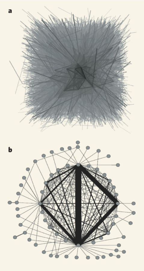
Figure 1: The interbank transfer network in 2007 The US interbank transfer network consists of over $6600$ financial institutions making over $70,000$ daily transfers. As mapped here from pre-financial crisis data, the network exhibits a pronounced core-halo structure (2a: reprinted with permission from reference [10]). The core of $66$ institutions (2b) includes an inner core of $25$ fully connected institutions, and accounts for $3/4$ of the transfer volume. As with the gravo-thermal catastrophe, a slowdown of the core can drive the entire system unstable, leading to the financial analogue of gravitational collapse (‘the black hole of finance’).

Like galaxies or nebulae, the interbank payment transfer network possesses a core-halo structure [10-11], and is susceptible to interaction-driven oscillation and instability. As detailed in [10], in 2007 this network consisted of over $6600$ financial institutions connected by over $70,000$ daily transfers. Most of the institutions (the halo) had either few links or links whose transfers had only small volume. A small, highly connected fraction of the institutions (the core), accounted for most of the volume. On a typical day, for example, a core of $66$ institutions connected by $181$ links comprised $75\%$ of the value transferred [10]. The core itself contained an ‘inner’ core of $25$ institutions that were almost fully connected. The core-halo structure of the network is shown in figure (1). Most important for stability analysis, the interbank payment transfer network is strongly disassortative [14]: highly-connected banks do most of their business with sparsely-connected banks, and vice versa. The disassortative nature of the network means that there are fewer internal links within the core, and within the halo, than there are between core and halo.

Disassortative networks are known to be less stable than assortative networks with respect to mixing and link removal [14]. The results of this paper can be applied to disassortative networks corresponding to the dynamics of coupled ordinary differential equations in general, and to the interbank transfer network in particular. Define a weighted disassortative network to be one in which the weighted sum of the links between highly connected core and the sparsely-connected halo is greater than the weighted sums of the links within the core and within the halo: $\sum_{i\in C,j\in H}|c_{ij}|^{2}>\sum_{ij\in C}|a_{ij}|^{2}+\sum_{ij\in H}|b_{ij}|^{2}$. Theorems 1 and 2 then imply

Theorem 3: A dynamical system whose gradient corresponds to a weighted disassortative network is either underdamped (with $\gamma>1$) or unstable.

Since the overall interbank network is disassortative, theorem 3 implies that stability/lack of oscillation can only be obtained when the banks in the core have significantly stronger interactions with each other than with banks in the halo. That is, even though the banks in the core undergo more transactions with banks in the halo than with each other, to maintain stability, typical flows between banks in the core and and other banks in the core must be significantly larger than typical flows between banks in the core and banks in the halo. This ‘hot core’ requirement for stability is confirmed by the data [10] – as noted, the core contains three quarters of the flow on a given day. Only by having large exchanges with each other (e.g., by hedging) can the banks within the core overcome the disassortative nature of the network to provide stability.

The hot core requirement leaves the network vulnerable to interaction-driven instability. Theorems 1 and 2 imply that if some event causes a sudden drop in the strength of transfer rates within the core, then the whole system can go unstable. The mathematical origin of this financial instability is the same as the origin of instability in gravo-thermal collapse, where a slowing of energy production in the core drives the system unstable. The end point of the financial instability is the well-known liquidity trap, a spectacular example of which occurred during the financial crisis of 2008-2009. For the bank transfer network, just as for black hole formation, instability leads to a collapsed regime in which the core freezes up, and transfers drop dramatically (‘the black hole of finance’).

Conclusion

This paper presented simple mathematical criteria for the stability and oscillatory behavior of dynamical systems as interactions are added between subsystems. If the number and strength of interactions between subsystems grows too large, the criteria identifies a threshold of connectivity beyond which oscillations and/or fluctuations inevitably grow. This result extends the May theorem for random networks to structured networks. A number of artificial and naturally occurring dynamical systems, such as the gravitational and financial systems discussed here, are subject to this threshold. Indeed, any system within which the number and strength of interactions increase over time, without an attending increase in the strength of local stabilizing dynamics, will inevitably approach the interaction oscillation/instability threshold. An interaction-driven core-halo instability lies at the heart of both financial and gravitational collapse. Once the instability threshold is passed, unless interactions between core and halo are reduced, and local stabilizing dynamics within the core and halo are increased, rapidly growing oscillations/fluctuations will overwhelm physical and financial stabilization mechanisms leading to gravitational and financial collapse.

Acknowledgments: This work was supported by a Miller fellowship from the Santa Fe Institute. The author would like to thank Olaf Dreyer, Jeffrey Epstein, Doyne Farmer, Thomas Lloyd, Cormac McCarthy, Sanjoy Mitter, Chris Moore, Sam Shepard, and Jean-Jacques Slotine for helpful conversations.

References

[1] D.G. Luenberger, Introduction to Dynamic Systems: Theory, Models and Applications, Wiley, New York, (1979).

[2] J.-J.E. Slotine, W. Li, Applied Nonlinear Control, Prentice Hall, Englewood Cliffs (1991).

[3] S. Strogatz, Nonlinear Dynamics and Chaos, Perseus Books, Cambridge (1994).

[4] R. May, Nature 238, 413 (1972).

[5] M. Newman, D. Watts, A.-L. Barabási, The Structure and Dynamics of Networks, (Princeton University Press, 2006).

[6] D. Angelis, Ecology 56, 238-243 (1975).

[7] D. Lynden-Bell, R. Wood, Mon. Not. R. Astr. Soc. 138, 495-525 (1968).

[8] M.P. Leubner, Astrophys. J. 604, 469 (2004).

[9] S. Nickerson, T. Csorgo, D. Kiang, Phys. Rev. C 57, 3251-3262 (1998); arXiv:nucl-th/9712059.

[10] K. Soramäki, M. L. Bech, J. Arnold, R.J. Glass, W.E. Beyeler, Physica A 379, 317-333 (2007).

[11] A.G. Haldane, R.M. May, Nature 469, 351-355 (2011).

[12] P. Krugman, The self-organizing economy, Blackwell, Oxford (1996).

[13] S.P. Borgatti, M.G. Everett, Soc. Net. 21, 375-395 (2000).

[14] M.E.J. Newman, SIAM Rev. 45, 167-256 (2003).

[15] R. Olfati-Sabera, R.M. Murray, IEEE Trans. Aut. Cont. 49, 1520-1533 (2004).

Supplementary material

Proof of theorem 1:

Let

$$G_{off}=\pmatrix{0&C\cr C^{\dagger}&0\cr}$$

be the off-diagonal part of the Hermitian gradient $G$. Similarly, let

$$G_{on}=\pmatrix{A&0\cr 0&B\cr}$$

be the on-diagonal part of $G$. The singular value decomposition for $C$ implies that the eigenvalues of $G_{off}$ are either zero, or come in pairs $\pm\lambda_{j}$, where the $\lambda_{j}\geq 0$ are the singular values of the matrix $C$. The $\pm\lambda_{j}$ eivenvectors of $G_{off}$ take the form $\vec{g}^{\pm}_{j}=\pmatrix{\vec{u}_{j}\cr\pm\vec{v}_{j}\cr}$, where $\vec{u}_{j}$ and $\vec{v}_{j}$ are the left-singular and right-singular vectors for $\lambda_{j}$: $C\vec{v}_{j}=\lambda_{j}\vec{u}_{j}$, $C^{\dagger}\vec{u}_{j}=\lambda_{j}\vec{v}_{j}$.

Now look at vectors of the form $\vec{w}=\pmatrix{\alpha\vec{u}_{j}\cr\beta\vec{v}_{j}\cr}$, where $\alpha,\beta$ are real and non-negative. Maximizing $\vec{w}^{\dagger}G\vec{w}$ over $\alpha,\beta$ yields $\vec{w}^{\dagger}G\vec{w}>0$ when $\lambda_{j}^{2}>a_{j}b_{j}$, where $a_{j}=\vec{u}_{j}^{\dagger}A\vec{u}_{j}$ and $b_{j}=\vec{v}_{j}^{\dagger}B\vec{v}_{j}$. So the system is unstable if $\lambda_{j}^{2}>a_{j}b_{j}$ for any $j$. In particular, if $\sum_{j}a_{j}b_{j}<\sum_{j}\lambda_{j}^{2}$, then the system is unstable.

Note that $a_{j}$, $b_{j}$ are the diagonal elements of $A$, $B$ in the bases $\{\vec{u}_{j}\}$ for $A$’s $n_{A}$-dimensional Hilbert space, and $\{\vec{v}_{j}\}$ for $B$’s $n_{B}$-dimensional Hilbert space. Let $\vec{\mu}$ be the vector of eigenvalues of $A$, and $\vec{\nu}$ be the vector of eigenvalues of $B$. It is straightforward to verify that the vectors $\vec{a}$ with components $a_{j}$ and $\vec{b}$ with components $b_{j}$ are related to $\vec{\mu}$ and $\vec{B}$ by doubly stochastic transformations: $\vec{a}=W_{A}\vec{\mu}$, $\vec{b}=W_{B}\vec{\nu}$. Convexity then implies that $|\vec{a}|^{2}=\sum_{j}a_{j}^{2}\leq|\vec{\mu}|^{2}=\sum_{j}\mu_{j}^{2}={\rm tr}A^{\dagger}A$. Similarly, $|\vec{b}|^{2}=\sum_{j}b_{j}^{2}\leq|\vec{\nu}|^{2}=\sum_{j}\nu_{j}^{2}={\rm tr}B^{\dagger}B$. These inequalities, combined with the Cauchy-Schwartz inequality, show that

$${\rm tr}C^{\dagger}C > \sqrt{{\rm tr}A^{\dagger}A}\sqrt{{\rm tr}B^{\dagger}B}$$

$$\longrightarrow\sum_{j}\lambda_{j}^{2} > |\vec{\mu}||\vec{\nu}|\geq|\vec{a}||\vec{b}|\geq\vec{a}\cdot\vec{b}=\sum_{j}a_{j}b_{j},\quad\quad\quad\quad(S2)$$

and the system is unstable. This proves the theorem.

Theorem 1 immediately implies a set of stability tests. Define $a^{2}=(1/n_{A}^{2}){\rm tr}A^{2}=(1/n_{A})\sqrt{\sum_{ij=1}^{n_{A}}|a_{ij}|^{2}}$ to be the average magnitude squared of the entries of $A$. $a$ can be thought of as the ‘strength’ of $A$’s stabilizing dynamics. Similarly, $b=(1/n_{B})\sqrt{{\rm tr}B^{2}}$ gives the ‘strength’ of $B$’s stabilizing dynamics, and $c=(1/\sqrt{n_{A}n_{B}})\sqrt{{\rm tr}C^{\dagger}C}$ is the strength of the potentially destabilizing dynamics of the interactions. Theorem 1 is equivalent to the statement that when $c^{2}>ab$, interactions cause instability: the system is unstable if the strength of the destabilizing interaction dynamics is greater than geometric mean of the strengths of the stabilizing local dynamics. Similarly, $c>(a+b)/2\geq\sqrt{ab}$, and $c^{2}>a^{2}/2+b^{2}/2\geq ab$ also imply instability.

The bound of theorem 1 is tight in the sense that for a given $C$, and fixed $a$, $b$ such that $ab>c^{2}$, the entries of $A$ and $B$ can always be chosen to make the system stable (bound (1c)). The ‘minimal’ strategy for attaining stability is align the eigenvectors of $A$ and $B$ with the left and right singular vectors of $C$. Arrange $\vec{\mu}\propto\vec{\nu}$, and $\mu_{j}\nu_{j}=\lambda_{j}^{2}+\epsilon$. Then the system is stable and

$$\sqrt{{\rm tr}A^{\dagger}A}\sqrt{{\rm tr}B^{\dagger}B}={\rm tr}C^{\dagger}C+O(\epsilon).$$

Similarly, the tight bounds (1a), (1b) can be attained by aligning the eigenvector of $G_{off}$ with the largest eigenvalue together with the eigenvectors of $A$,$B$ with the smallest eigenvalue product.

Proof of theorem 2:

First, look at the oscillatory behavior of the matrix

$$G^{\prime}=\pmatrix{A&\tilde{C}\cr-\tilde{C}^{\dagger}&B\cr}$$

that contains the Hermitian gradients for the on-diagonal terms and the anti-Hermitian gradient for the interaction terms. We will show that theorem 2 holds for this gradient. As will be seen, adding the anti-Hermitian parts of the on-diagonal terms and the Hermitian parts of of the interaction terms cannot decrease the damping ratio.

Use the same analysis as in theorem 1. Now let $\vec{u}_{j}$ and $\vec{v}_{j}$ be the left-singular and right-singular vectors for $\tilde{C}$ with singular value $\lambda_{j}$. The eigenvectors of $G^{\prime}_{off}=\pmatrix{0&\tilde{C}\cr\tilde{C}^{\dagger}&0\cr}$ now take the form $\vec{g}^{\pm}_{j}=\pmatrix{\vec{u}_{j}\cr\pm i\vec{v}_{j}\cr}$ with eigenvalues $\pm i\lambda_{j}$. In analogy to the proof of theorem 1, look at vectors of the form $\vec{w}=\pmatrix{\alpha\vec{u}_{j}\cr i\beta\vec{v}_{j}\cr}$, where $\alpha,\beta$ are real. Maximizing the damping ratio $|\vec{w}^{\dagger}G^{\prime}_{off}\vec{w}|/|\vec{w}^{\dagger}G^{\prime}_{on}\vec{w}|$ over $\alpha,\beta$ yields a value $\gamma=\lambda_{j}/\sqrt{a_{j}b_{j}}$, where as before $a_{j}=\vec{u}_{j}^{\dagger}A\vec{u}_{j}$ and $b_{j}=\vec{v}_{j}^{\dagger}B\vec{v}_{j}$. Following the proof of theorem 1, we see that when ${\rm tr}\tilde{C}^{\dagger}\tilde{C}\geq\gamma^{2}\sqrt{{\rm tr}A^{2}}\sqrt{{\rm tr}B^{2}}$ the damping ratio for the state $\vec{w}$ is equal to $\gamma$. This proves the theorem for matrices of the form $G^{\prime}$. Adding the anti-Hermitian parts of the diagonal terms can only increase the magnitude of the numerator of the damping ratio, while adding the Hermitian parts of the off-diagonal, interaction terms can only decrease the minimum value of the denominator. Indeed, including the Hermitian part of the off-diagonal term $G_{off}$ and performing the optimization above yields a tighter bound: oscillation occurs with damping ratio $>\gamma$ if

$${\rm tr}~{}\tilde{C}^{\dagger}\tilde{C}>\gamma^{2}(2\sqrt{{\rm tr}A^{2}{\rm tr}B^{2}}-|{\vec{g}^{+}_{j}}{{}^{\dagger}}G_{off}\vec{g}^{+}_{j}|)^{2}.$$

So theorem 2 holds for all gradients $\nabla g$.

Tight bounds for the oscillatory threshold are attained in analogue to (1a), (1b), (1c) by aligning the ‘strongest’ and ‘weakest’ eigenvector/eigenvalue combinations of $A$, $B$, and $\tilde{C}$.

Linearized equations for the gravo-thermal catastrophe:

Consider a system bound together by gravitation such as a star, nebula, or galaxy. Such systems typically possess a core-halo structure [7]. Let $E_{A}$, $T_{A}$ be the energy and temperature of the core, and $C_{A}$ its specific heat. Similarly, let $E_{B}$, $T_{B}$ and $C_{B}$ be the energy, temperature and specific heat of the halo. $\alpha\geq 0$ gives the linearized rate of energy transfer between core and halo as a function of their temperature difference. $\eta\geq 0$ governs heat production in the core, due, e.g., to nuclear reactions, and $\zeta\geq 0$ governs heat loss from the halo to space beyond. The linearized equations of motion are

$${dE_{A}\over dt}=C_{A}{dT_{A}\over dt}=\alpha(T_{B}-T_{A})+\eta T_{A},\quad{dE_{B}\over dt}=C_{B}{dT_{B}\over dt}=\alpha(T_{A}-T_{B})-\zeta T_{B}.$$

Eliminating $E_{A},E_{B}$ then yields equation (6) of the text.

Instability of the bank transfer network:

To derive the interaction-driven instability threshold for the bank transfer network, divide the network into the set of banks with above-average numbers of links and volumes (the core, system ${\cal A}$), and those with below average numbers of links and volumes (the halo, system ${\cal B}$). Let $v_{ij}$ be the measured volume flow from bank $j$ to bank $i$ during a particular reporting period. To construct a linearized dynamics would require knowledge of $V_{j}$, the amount of funds held in bank $j$, together with the rates $v_{jj}$ of creation and consumption of funds within the $j$’th bank. These numbers are not available from the data set analyzed in [10]. Even though $V_{j}$ and $v_{jj}$ are unknown, however, the stability analysis of theorems 1 and 2 can still be applied.

In the linearized dynamics, the gradient matrix $\nabla g$ has entries $v_{ij}/V_{j}$. The matrices $A$,$B$, $C$, and $\tilde{C}$ are derived from $\nabla g$ as before: $A$ governs the Hermitian dynamics within the core, $B$ governs the dynamics within the halo, and $C$,$\tilde{C}$ govern flows between core and halo. Let $\kappa_{A}$ be the fraction of non-zero terms within $A$, so that $\kappa_{A}n_{A}^{2}$ is the number of links within the core. Define $\kappa_{B}$ and $\kappa_{C}$ in the same way. Let $\bar{a}^{2}$ be the average magnitude squared of a non-zero term in $A$: $\bar{a}^{2}=a^{2}/\kappa_{A}$, where as above $a=(1/n_{A})\sqrt{{\rm tr}A^{\dagger}A}$ is the average strength of all the terms in $A$, including those that are zero. Similarly, $\bar{b}^{2}=b^{2}/\kappa_{B}$, $\bar{c}^{2}=c^{2}/\kappa_{C}$ are the average magnitude squared of non-zero terms in $B$ and $C$. Theorem 1 then implies that the dynamics are unstable if

$$\kappa_{C}\bar{c}^{2}>\sqrt{\kappa_{A}\kappa_{B}}\bar{a}\bar{b}.$$

Similarly, theorem 2 implies that the dynamics exibit oscillations with underdamping degree $>\gamma$ if

$$\kappa_{\tilde{C}}\bar{\tilde{c}}^{2}>\gamma^{2}\sqrt{\kappa_{A}\kappa_{B}}\bar{a}\bar{b}.$$

The disassortative nature of the network [10] now sets the stage for connectivity-driven oscillations and instability: when the strength of internal stabilizing dynamics is insufficient, the dynamics of the network gives rise to oscillatory and/or unstable flows between core and halo. The disassortative nature of the network implies that there are fewer internal links within the core, $\kappa_{A}n_{A}^{2}$, and within the halo, $\kappa_{B}n_{B}^{2}$, than there are between core and halo, $\kappa_{C}n_{A}n_{B}$. That is, disassortativity implies $\kappa_{C}^{2}>\kappa_{A}\kappa_{B}$. Equations (S6) and (S7) then imply theorem 3. In a core-halo system, stability requires that the strength of links within the core be significantly higher than the strength of links between core and halo, a feature observed in the actual bank transfer network (3/4 of the volume of transfers occurs within the core).

If the system is marginally stable, so that $\kappa_{C}\tilde{c}^{2}\approx\sqrt{\kappa_{A}\kappa_{B}}\tilde{a}\tilde{b},$ then any dip in the connectivity or the strength of connections within the core will drive it unstable.