Bridging stylized facts in finance and data non-stationarities

Abstract

Employing a recent technique which allows the representation of nonstationary data by means of a juxtaposition of locally stationary paths of different length, we introduce a comprehensive analysis of the key observables in a financial market: the trading volume and the price fluctuations. From the segmentation procedure we are able to introduce a quantitative description of statistical features of these two quantities, which are often named stylized facts, namely the tails of the distribution of trading volume and price fluctuations and a dynamics compatible with the U-shaped profile of the volume in a trading section and the slow decay of the autocorrelation function. The segmentation of the trading volume series provides evidence of slow evolution of the fluctuating parameters of each patch, pointing to the mixing scenario. Assuming that long-term features are the outcome of a statistical mixture of simple local forms, we test and compare different probability density functions to provide the long-term distribution of the trading volume, concluding that the log-normal gives the best agreement with the empirical distribution. Moreover, the segmentation of the magnitude price fluctuations are quite different from the results for the trading volume, indicating that changes in the statistics of price fluctuations occur at a faster scale than in the case of trading volume.

1 Introduction

In the last decades, the description of dynamic and statistical quantities related to Finance has turned into an appealing subject for the exploration of physical concepts beyond the scope they were originally introduced to books . Much of the effort has been put upon shedding light on trust- worthy mechanisms leading to the emergence of power-law distributions, e.g., for the log-price fluctuations the distribution of which exhibits an asymptotic scale-invariant form with slow convergence to the Gaussian, with the Berry-Esséen theorem defining the upper limit of difference between obtained and expected cummulative distribution functions be . It is well established that the changes in the share price are triggered by a myriad of factors (previous price fluctuations, deviations from the target price, news, etc.) that make some people willing to buy and some other to sell. Moreover, activity of a financial market is non-stationary lux ; bertram ; scalas ; marsili ; livan . To this trait it was assigned the origin of fat tails in financial observables like the trading volume tailvol ; epl-vol ; celia-vol , which on its turn would imply fat tails in the price fluctuations and on volatility as well volvol . This scenario abides by the Wall Street heuristic law disseminated by Karpoff’s work that it takes volume to make price move karpoff .

In both Physics and Finance, the treatment of non-stationary data is often tackled assuming sets of coupled stochastic differential equations representing different scales of evolution of the system, which frequently pave the way to demanding solutions multiscale . Mixtures of stochastic processes, e.g., compound Poisson processes, can also be considered scalas . However, allowing for the fact that to fit real data some of these equations must have large relaxation times, the modeling of non-stationary quantities can be efficiently simplified by considering that the system is in a generic steady state regime and the data are well described by a juxtaposition of intervals of length $\ell$ characterized by few $N$ parameters $\left\{\pi\right\}$ beck . At the scale $\ell$, the parameters are assumed constant, but in the long-term follow a certain probability density function. Within this approach, the length of the local patches $\ell$ is systematically constant as well. This time independence can only be understood as the first order of the juxtaposition approach, because it is unlikely that complex systems are so well behaved in this respect. Furthermore, it is intuitive to think that a dynamics for the length of the regions of local stationarity contains valuable information with respect to overall features of the observable, e.g., the evolution of the correlations. In addition, we can look at the outcome of the single scale proposal as a (new) mixture of ‘cut and pasted’ elementary scales that screens the actual statistical nature of the local parameters, in the context of what was called superstatistics by Beck and Cohen beck-cohen .

Recently, a work of ours introduced a non-parametric segmentation procedure, dubbed Kolmogorov-Smirnov segmentation (KSS) kss , aimed at defining quasi-stationary segments of varying length in non-stationary time series (see A). Although the non-uniform segmentation of non-stationary time series was not a brand new approach to the problem montoro , KSS clearly outperforms previous approaches to the problem that use either local moments testing or principal component analysis in accuracy or fastness compete1 ; compete2 ; compete3 .

Generically, the hypothesis that the length of the segments of local stationarity is not constant sets the scene for a real dependence between the values of the local parameters $\left\{\pi\right\}$ and the duration $\ell$ of the patches. Therefore, the long-term distribution of observable $\mathcal{O}$ within this framework is given by

$$P\left(\mathcal{O}\right)=\int\ldots\int p\left(\mathcal{O};\left\{\pi\right\},\ell\right)\,p_{\pi}\left(\left\{\pi\right\};\ell\right)\,p_{\ell}\left(\ell\right)\,d\pi_{1}\ldots d\pi_{n}\,d\ell$$ (1)

where $p\left(\mathcal{O};\left\{\pi\right\},\ell\right)$ represents the conditional probability of having a value $\mathcal{O}$ given local parameters $\left\{\pi\right\}$ in a segment of length $\ell$. Assuming $p_{\ell}\left(\ell\right)=\delta\left(\ell-\lambda\right)$ we get the constant $\ell$ case.

After obtaining clear-cut results on heart-rate variability and atmospheric turbulence kss , we investigate the impact of the non-stationary nature of financial time series in a large set of stylized facts. Specifically, from a thorough characterization of the features of the trading volume at short time scales (1 minute), we pitch at describing not only its statistical properties but also at introducing a proper representation of price fluctuations from statistical properties of trading volume as first endeavoured using daily data osborne and more recently essayed in baltic using coupled equations. Concretely, our analysis focus on the dataset composed of price fluctuations, $r_{i}(t)\equiv S_{i}(t)-S_{i}(t-1)$, and the trading volume, $V(t)$, of the 30 blue chip companies defining the Dow Jones Industrial Average recorded at every 1 minute during the second semester of 2004. This corresponds to circa $5\times 10^{4}$ data points for each quantity of every stock $i$. For the sake of handleness we have normalized the trading volume of each stock by its average value over the span $v_{i}(t)\equiv V_{i}(t)/\overline{V_{i}}$. The price fluctuations (or returns) were kept as defined.

2 Heterogeneities in trading volume

2.1 Statistics of the patches

As we want to describe established key facts and statistical features of financial markets from trading volume, we start our analysis by applying the KSS algorithm to this last quantity. Despite working nicely without the need for any additional constraint, e.g., a lower bound for the size of the segments, we curbed the length $\ell$ to a minimum of $30$ minutes. This is the time scale describing a first regime of the autocorrelation function of the trading volume that was found not only for this same data but also for data from other markets celia-vol ; epjb-vol . It is worth mentioning that the introduction of this lower bound does not affect the results we present hereinafter, namely the typical length of the segments of quasi-stationarity. 

Let us first describe the probability density function (PDF) of the duration of the patches. From a first visual inspection of Fig. 1, we noticed there is a well defined exponential regime,

$$P_{\ell}\left(x>\ell\right)=\exp\left[-\frac{\ell-\ell_{\min}}{\lambda}\right],$$ (2)

which accounts for more that $95\%$ of the empirical distribution. Because each firm presents as much as 300 segments, the remaining $5\%$ of the empirical complementary cumulative distribution function (EDF), which describes around 15 segments for each set, is strongly affected by the finiteness of the patches set. It is thus tempting to consider the change in the behavior of the curve a simple artifact. However, we do not have a random modification. Instead, we observe a consistent decrease of its absolute value for all the stocks and also that the changes come to pass at the same length $\ell\sim 330$ minutes. Therefore, we reckon there exists a second regime in the length of stationary segments, which rules the statistics of patches that last longer than a trading session.

Concentrating our efforts on the significant part of the distribution, we used a log-likelihood adjustment procedure and from it we consistently found that the EDFs fit for Eq. (2) with similar values for all the stocks. The the average value, $\left\langle\lambda\right\rangle$, is equal to $116\pm 12\,\,\min$, when Microsoft (MSFT) is set aside ($\left\langle\ldots\right\rangle$ stands for averages over companies). For Microsoft, we have found a typical scale of 230 minutes, which is quite different from the remaining values even when we compare it with $\lambda=120$ minutes of Intel (INT), which is also traded at NASDAQ and that agrees with $\left\langle\lambda\right\rangle$. The empirical distribution function of $\ell$ is shown in Fig. 1. The reader should pay attention to the fact that despite we did not remove overnight effects, which might affect a financial data analysis, our characteristic time scale of local stationarity is significantly smaller than the span of a trading session. Moreover, should the trading span influence our result, then there would be a separation between NYSE and NASDAQ traded stocks, which is not the case bearing in mind Intel time scale.

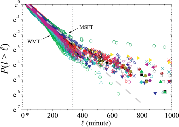
Figure 1: Complementary cumulative distribution function $P\left(\ell\right)$ vs segment length $\ell$ for the companies of the DJIA index in a $\ln$-linear scale. Apart from the deviation in the tail a typical exponential decay is apprehended. In the plot, we indicate the companies with the shortest characteristic scale, Walmart (WMT), and the company with the longest characteristic scale, Microsoft (MSFT).

The next logical step is to verify whether the length of the segments are related to one another. This is appraised by looking into the behavior of the fluctuations,

$$\Delta\ell_{j}\left(i\right)=\ell_{i+j}-\ell_{i}.$$ (3)

Already for immediate segments, $j=1$, we found white noise correlations,

$$C_{\Delta\ell_{1}}\sim\left\langle\Delta\ell_{1}\left(i+l\right)\Delta\ell_{1}\left(i\right)\right\rangle-\left\langle\Delta\ell_{1}\right\rangle^{2}=\delta_{l,0}.$$ (4)

However, when we analysed the correlation function of $|\Delta\ell_{1}|$, we verified that it takes a lag around 4 segments to attain noise level, which using the value of $\left\langle\lambda\right\rangle$ is close to the span of a trading session.

Considering high-frequency trading volume, it is known that markets tend to exhibit high level of activity during the beginning and during the end of the trading sessions u-shape . Therefore, the KSS must yield indications of that U-shape profile of the trading volume within a trading session, beyond the first indications that the $C_{|\Delta\ell_{1}|}$ behavior is alluding to. We first looked for a relation between the size of the segments, $\ell$, and its average value of trading volume, $\mu_{\ell}$. Although the plots $\ell$ versus $\mu$ are somewhat sprinkled (see Fig. 2), recurring to a standard statistical technique of local regression (see App. B), we were able to verify that there is an inverse relation $\ell$ and $\mu_{\ell}$ that goes beyond statistical error due to sample size. This result is plausible because it is likely that periods with little activity (or small $\mu$) last longer and that periods of high activity (or large $\mu$) induce changes in the activity level more easily so that the local stationarity condition is also more easily violated.

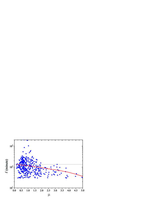
Figure 2: Typical dependence of the size of the segment of local stationarity, $\ell$, vs local average value of the trading volume, $\mu$, for General Electric. The line represents the local adjustment given by loess algorithm (see App. B).

With the goal of understanding how the segments length distributes within each intra-day trading hour, we have looked at the starting time of each segment of local stationarity and afterwards we coarse grained them in such a way that the probability of obtaining a given band is always equal to $1/8$. Accordingly, if the distribution of segments was completely uniform along the day, then these probabilities would not vary (within error bars).

Taking into account the stack column bar plot in Fig. 3, we noted that there is in fact an intra-day dynamics for the conditional fraction of the segments length. First, we apprehended that short and long segments exhibit complementary behavior, i.e., longer segments have their higher probability of starting during the first hours of a trading session, perhaps reflecting trading sessions without much ado. After that, it decreases to values smaller than $1/8$ from the second hour of trading onwards, which indicates a strong intraday dynamics that moves on into further sessions. For the smaller segments, we have almost the same probability, which increases as the terminus of the session comes up. We relate this behavior to the practice of cleaning the order book as the session approaches its end. With a similar dependence there is a second group of segments of intermediate length, but for which the final surging is very pronounced. The distinctive behavior with the trading time can be already understood from these two analyses.

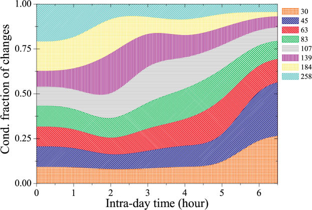
Figure 3: Averaged stack column bar plot of the conditional probability of having a change of local regime which lasts for $\ell$ minutes averaged over all companies and the frontiers are smoothed using a B-spline. The values of the legend represent the initial value of each interval grouping.

Furthermore, to separate out the beginning of the session from the subsequent hours, we appraised to what extent segments distribute within the trading session regardless their length. Figure 4 shows that changes of local stationarity occur less in the middle of the session. Combining the analysis of Figs. 3-4 we perceive a dynamics totally compatible with the aforestated U-shape in the trading volume.

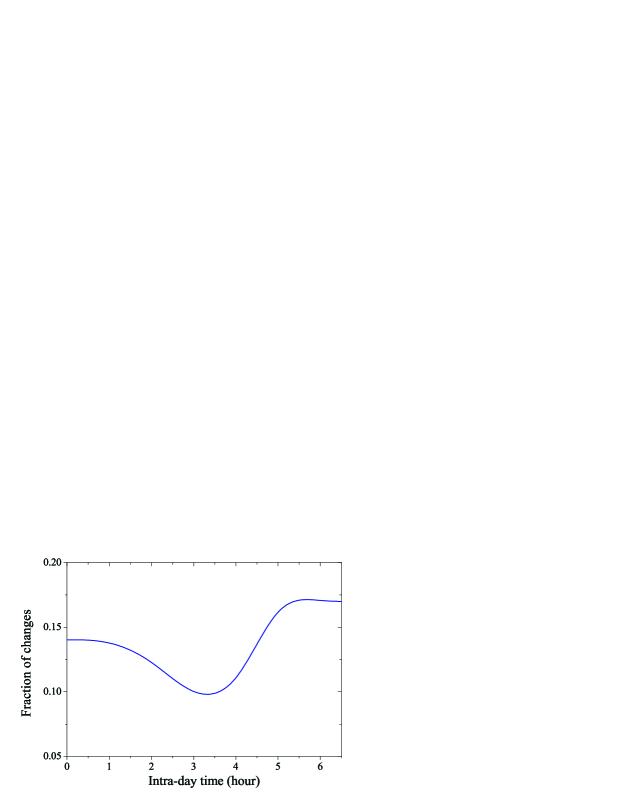
Figure 4: Averaged probability of having a change of local stationarity for a given intra-day time smoothed using a B-spline.

An important point in the mixing scenario is that of the slow evolution of the fluctuating parameters that we fix within each patch. In Fig. 5, we show the average behavior of the correlation function of sequence of average local values of the trading volume, $\mu$, values as a function of the lag defined in number of segments units,

$$C_{\mu}\sim\left\langle\mu\left(i+l\right)\,\mu\left(i\right)\right\rangle-\left\langle\mu\right\rangle^{2}.$$ (5)

Therein, it is visible that it takes as much as $18$ segments to have the correlation at the noise level, which correctly accommodates in the mixing approach. Interestingly, we noted the existence of a bounce back of the value of $C_{\mu}$ at $l=3$ which is dimly repeated at $l=4$ intervals until noise level is reached. A similar curve is found when the auto-correlation of the trading volume is analyzed. In other words, in segmenting the series using the KSS algorithm, we preserved the long-term correlation function that also signals the typical scale equal to the duration of a trading session which is close to 4 segments of average length.

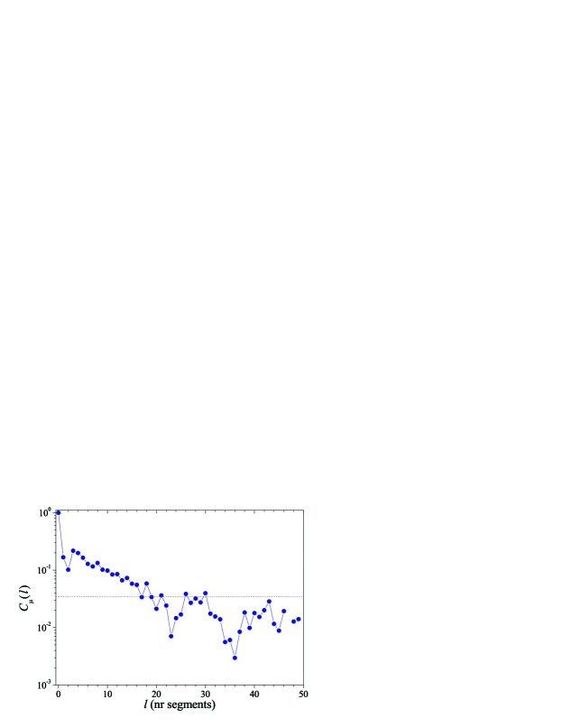
Figure 5: The averaged correlation function of the local mean value of the trading volume vs the lag measured in segments. The horizontal dashed line represents the noise level. Looking to the symbols we verify that $C_{\mu}\left(l\right)$ reaches the noise level for a lag around five days. Interestingly, we notice the intra-day signature for the bouncing back of $C_{\mu}$ at $l=3$ followed by other weaker and dwindling rallies at $l=4$ intervals until the noise level is attained.

2.2 Long-term behavior from the local statistics of trading volume

With the segmentation in hand and a first group of well-known properties matching the segmentation results, we moved ahead into probabilistic features. Owing to the assumption that the long-term behavior is the outcome of a statistical mixture of simple local forms, we assessed the statistical hypothesis that the trading volume is locally described by one of these simple two-parameter PDFs: the $\Gamma$-distribution,

$$p_{\Gamma}\left(v;\left\{\phi,\theta\right\}\right)=\frac{v^{\phi-1}}{\theta^{\phi}\,\Gamma\left[\phi\right]}\exp\left[-\frac{v}{\theta}\right],$$ (6)

the log-Normal distribution,

$$p_{\mathrm{lN}}\left(v;\left\{\phi,\theta\right\}\right)=\frac{1}{\sqrt{2\,\pi}\theta\,v}\exp\left[-\frac{\left(\ln v-\phi\right)^{2}}{2\,\theta^{2}}\right],$$ (7)

the inverse $\Gamma$-distribution,

$$p_{\mathrm{i}\Gamma}\left(v;\left\{\phi,\theta\right\}\right)=\frac{\theta^{\phi}}{\,\Gamma\left[\phi\right]}v^{-\phi-1}\exp\left[-\frac{\theta}{v}\right],$$ (8)

and Weibull distribution,

$$p_{W}\left(v;\left\{\phi,\theta\right\}\right)=\frac{\phi}{\theta^{\phi}}v^{\phi-1}\exp\left[-\left(\frac{v}{\theta}\right)^{\phi}\right].$$ (9)

We proceeded as follows: for every stock we have considered the segments obtained by the KSS and looked for the best local fit for PDFs (6)-(9) by means of optmizing the respective log-likelihood function. Subsequently, we checked the statistical significance of each fit considering the quantity $\sqrt{\ell}\,d_{\max}$, where $d_{\max}$ is the maximum distance between the EDF and the fitting cummulative distribution function assuming a Lilliefors approach. From this procedure, we learnt that the log-normal distribution presents the smallest value $\langle\sqrt{\ell}\,d_{\max}\rangle_{i}=0.82\pm 0.06$, with the other distributions yielding average results greater than one ($\langle\ldots\rangle_{i}$ stands for average over all the segments of company $i$).

Alternatively, having applied the Kolmogorov-Smirnov statistical distance criterion with an $\alpha$-value equal to $0.05$ to each segment for each testing distribution, we found an average ratio of statistical significance equal to $0.95\pm 0.04$ for the log-Normal. For the remaining test distribution we got a statistical significance ratio equal to $0.78\pm 0.06$ for the $\Gamma-$distribution and $0.81\pm 0.04$ for the Weibull distributions. Once more, the worst fit is for the inverse $\Gamma$-distribution, which gave $0.41\pm 0.09$, i.e., a performance ratio below $1/2$. The good results of the $\Gamma$-distribution underpin the previous approach of a local Feller process epl-vol ; celia-vol ; jstat-vol .

An individual analysis of the companies also shows that the log-Normal tested as the best local distribution for all the 30 stocks and the inverse $\Gamma$-distribution the worst of the test hypotheses.

As previously denoted by Eq. (1), the long-term distribution is the result of a local statistics, $p\left(v;\left\{\phi,\theta\right\}\right)$, that is weighed taking into consideration the statistics of $\phi$ and $\theta$, $g\left(\phi,\theta\right)$. Let us start reporting how $\theta$ is distributed. To tackle this point, we compared the test distributions by computing $\sqrt{n}\,d_{\max}$, where $d_{\max}$ is again the maximal distance between the EDF and each of the complementary cumulative distribution function after a log-likelihood adjustment and $n$ the number of $\theta$ values in the set, i.e., the number of segments we obtained each stock. The averages over all the companies and medians of $\sqrt{n}\,d_{\max}$ are,

$$\begin{array}[]{cccc}&\left\langle\sqrt{n}d_{\max}\right\rangle&&(\sqrt{n}\widetilde{d_{\max}})\vspace{0.15cm}\\ \Gamma\textrm{-distribution:}&1.05\pm 0.58&&0.95\vspace{0.05cm}\\ \textrm{inverse}\;\Gamma\textrm{-distribution:}&1.39\pm 0.47&&1.35\vspace{0.05cm}\\ \textrm{log-Normal:}&4.94\pm 2.27&&5.09\vspace{0.05cm}\\ \textrm{Weibull:}&1.13\pm 0.54&&1.10\vspace{0.05cm}\\ \textrm{inverse}\,\textrm{Weibull:}&2.15\pm 0.54&&2.16\end{array}$$

showing that the distribution which better describes the long term behavior is the $\Gamma$-distribution. Looking more attentively at the results, we perceived different behavior for NYSE and NASDAQ traded stocks. For the former, $p\left(\theta;\left\{\gamma,\kappa\right\}\right)$ is best described by Eq. (6) with average values $\gamma=32.8\pm 4.7$ and $\kappa=0.028\pm 0.004$ and medians equal to $32.3$ and $0.028$, respectively. Then again, for Intel and Microsoft, the best fit $p\left(\theta;\left\{\gamma,\kappa\right\}\right)$ is given by Eq. (9) with similar exponent and scaling parameters for both the stocks, namely $\left\{\gamma=3.25,\kappa=1.26\right\}$ and $\left\{\gamma=2.86,\kappa=1.19\right\}$. The values of the parameters $\gamma$ and $\kappa$ of NYSE companies gave on average $\theta$ equal to $0.92\pm 0.14$ and a standard deviation equal to $0.16\pm 0.02$ while for Intel and Microsoft we have $1.13\pm 0.38$ and $1.06\pm 0.40$, respectively. It is worth remembering that we have normalized our finite series of trading volume dividing each one by its average value.

The problem of the PDF of $\phi$ is very much simplified by another empirical finding of ours. In performing a scatter plot of the local average, $\mu_{l}\equiv\bar{v}_{l}$, versus the local variance, $\omega_{l}\equiv\overline{v^{2}}_{l}-\bar{v}_{l}^{2}$, we perceived a clear dependence between these two moments. Setting the scatter plot in a $\ln-\ln$ scale, Fig. 6 shows that this dependence is close to a dual linear relation,

$$\ln\mu_{l} = \left\{\alpha^{\left(>\right)}\ln\omega_{l}+\eta^{\prime\left(>\right)}\right\}\,\Theta\left[\ln\omega_{l}-\Omega\right]$$

$$+\left\{\alpha^{\left(<\right)}\ln\omega_{l}+\eta^{\prime\left(<\right)}\right\}\,\Theta\left[\Omega-\ln\omega_{l}\right],$$

with,

$$\Omega\equiv\frac{\alpha^{\left(<\right)}-\alpha^{\left(>\right)}}{\beta^{\left(>\right)}-\beta^{\left(<\right)}},$$ (11)

where $\Theta$ is the Heaviside function and $\eta^{\prime\left(\gtrless\right)}\equiv\beta^{\left(\gtrless\right)}+\eta^{\left(\gtrless\right)}$ (for the sake of conciseness we omitted the dependence of $\mu_{l}$ and $\omega_{l}$ on $\phi$ and $\theta$). The variable $\Omega$ represents the value at which we obtained a crossover and $\eta^{\left(\gtrless\right)}$ is Gaussian distributed with standard deviation $\sigma_{\eta^{\left(\gtrless\right)}}$ and null mean. For all the companies, except 3M, the crossover dependence Eq. (2.2) was found with $\left\langle\mu_{l}\left(\Omega\right)\right\rangle=1.23\pm 0.88$. This suggests the existence of a regime for smaller and another one for larger trading volumes, as a previous scaling analyses suggested scaling . Regarding the remaining parameters we obtained the following values above and below $\Omega$,

$$\begin{array}[]{ccc}\alpha:&0.24\pm 0.08,&0.45\pm 0.05;\vspace{0.05cm}\\ \beta:&0.22\pm 0.19,&0.03\pm 0.11;\vspace{0.05cm}\\ \sigma_{\eta}:&0.39\pm 0.08,&0.28\pm 0.05.\vspace{0.05cm}\end{array}$$ (12)

As regards the median, which is less sensitive to extreme values we got: $\widetilde{\alpha^{\left(\gtrless\right)}}=\left\{0.23,0.44\right\}$, $\widetilde{\beta^{\left(\gtrless\right)}}=\left\{0.22,0.02\right\}$, $\widetilde{\sigma_{\eta^{\left(\gtrless\right)}}}=\left\{0.37,0.26\right\}$. Two notes on the relation between $\omega_{\ell}$ and $\mu_{\ell}$ are still worthwhile: first, we tried adjusting the scatter plot with a 2nd order polynomial, but the results were clearly worse; second, although the dual relation provides a better description of the data, a simple power-law adjustment fits the points fairly well, as shown by the dotted line in Fig. 6.

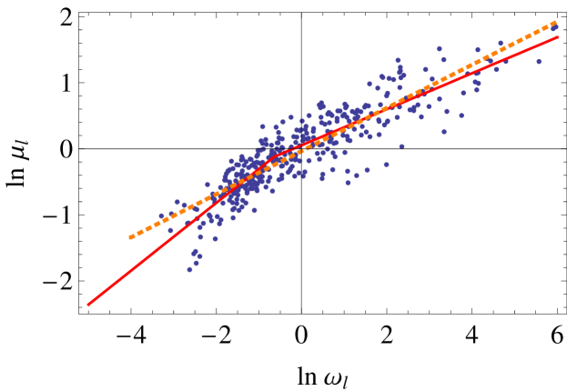
Figure 6: Scatter plot of $\ln$ $\mu_{l}$ vs $\ln\,\omega_{l}$ for General Electric. The full line represents a numerical adjustment with Eq. (2.2) and the dotted line is a simple power-law.

For a log-Normal distribution defined by the parameters $\phi$ and $\theta$, the mean and the variance are equal to,

$$\mu=\exp\left[\phi+\frac{\theta^{2}}{2}\right],$$ (13)

and,

$$\omega=\left(\exp\left[\theta^{2}\right]-1\right)\exp\left[2\,\phi+\theta^{2}\right],$$ (14)

respectively. Using these two equalities, we get for $\Omega=\pm\infty$,

$$\phi=\frac{\beta}{1-2\alpha}-\frac{\theta^{2}}{2}+\frac{\alpha\,\ln\left[\exp\left[\theta^{2}\right]-1\right]}{1-2\alpha}.$$ (15)

While for the case of the dual-linear relation, it is not hard to obtain the equation yielding the crossover parameters $\phi_{c}$ and $\theta_{c}$,

$$\left\{\begin{array}[]{c}\phi_{c}+\frac{\theta_{c}^{2}}{2}=\frac{\alpha^{<}\beta^{>}-\alpha^{>}\beta^{<}}{\beta^{>}-\beta^{<}}\,,\\ \\ 2\,\phi_{c}+\theta_{c}^{2}\ln\left[\exp\left[\theta_{c}^{2}\right]-1\right]=\Omega\,,\end{array}\right.\vspace{0.1cm}$$ (16)

it is very hard to obtain a simple expression analogue to Eq. (15), namely $\phi\left(\theta;\phi_{c},\theta_{c}\right)$. Moreover, despite the fact that the fits using Eq. (2.2) are better than a simple power-law and also that this dual approach also helps verify previous results over disparities between small and large trading volume, the approach based on Eq. (2.2) drags in additional complications, particularly when one wants to apply fast numerical integration methods such as the global adaptive strategy algorithm numint .

Bringing together all these findings, the long-term distribution of trading volume is finally obtained performing the integration,

$$P\left(v\right) = \int\int p\left(v|\phi,\theta\right)\,f\left(\phi,\theta,\ell\right)\,d\phi\,d\theta\,d\ell$$

$$= \int\int\int_{\ell_{\min}}^{\infty}F_{\ell}\left[\mu\left(\phi,\theta\right)\right]\,g\left(\theta\right)\,\,f_{\ell}\left(\ell\right)\,p\left(v|\phi,\theta\right)\,f\left(\phi|\theta\right)\,d\phi\,d\theta\,d\ell$$

where,

$$p\left(v|\phi,\theta\right)=\frac{1}{\sqrt{2\pi}\theta\,v}\exp\left[-\frac{\left(\ln v-\phi\right)^{2}}{2\,\theta^{2}}\right],$$ (18)

expresses the local log-Normal dependence of the trade volume. The function

$$f\left(\phi|\theta\right)=\delta\left(\phi-\left[\frac{\beta}{1-2\alpha}-\frac{\theta^{2}}{2}+\frac{\alpha\,\ln\left(\exp\left[\theta^{2}\right]-1\right)}{1-2\alpha}\right]\right)$$ (19)

embodies the dependence between local average and local standard deviation. The function $F_{\ell}\left[\mu\left(\phi,\theta\right)\right]$ is a Dirac delta functional similar to Eq. (19) that allows writing the length of a segment, $\ell$, as a function of local parameters $\phi$ and $\theta$ via the local value of $\mu$ given by Eq. (13), namely

$$F_{\ell}\left[\mu\left(\phi,\theta\right)\right]\equiv\delta\left[\ell-h\left(\exp\left[\phi+\frac{\theta^{2}}{2}\right]\right)\right],$$ (20)

where the function $h\left(x\right)$ represents the fit for the loess curves $\ell$ vs $\mu$ (see, e.g., Fig. 2) with its argument, $\mu$, substituted for primary parameters $\phi$ and $\theta$ in accordance with Eq. (13). According to what we said, the distribution of $\theta$ is given by,

$$g\left(\theta\right)=\frac{\theta^{\gamma-1}}{\kappa^{\gamma}\,\Gamma\left[\gamma\right]}\exp\left[-\frac{\theta}{\kappa}\right],$$ (21)

and finally $f_{\ell}\left(\ell\right)$ is given by Eq. (2).

Haplessly, the analytical determination of Eq. (2.2) is not possible in this case. In respect of a numerical solution we can do it twofold. In the first case, we assume that the length of a segment and the local moments are independent and that the relation between $\ln\mu$ and $\ln\omega$ is linear. Alternatively, one can appraise out the mixing scenario considering a weighed mixture of the $n$ local log-Normal distributions defined by local parameters $\phi_{i}$ and $\theta_{i}$, wherein the relative length of the $i$-th segment, $\ell_{i}/L$, plays the role of the weight,

$$P\left(v\right)\simeq\frac{1}{L}\sum_{i=1}^{n}\ell_{i}\frac{1}{\sqrt{2\,\pi}\theta_{i}\,v}\exp\left[-\frac{\left(\ln v-\phi_{i}\right)^{2}}{2\,\theta_{i}^{2}}\right],$$ (22)

($L$ is the length of the time series). As understood in Fig. 7, despite the simplifications both approaches already yield a good agreement for small, central and large values of the trading volume. This is particularly clear for the latter case in which we basically do not assume any approximation. In this case, we also implicitly benefit of using information on the finiteness of the data, whereas Eq. (2.2) assumes an infinitely long time series and neglects the local average – segment length relation, which explains the better results given by the green dashed curves in Fig. 7.

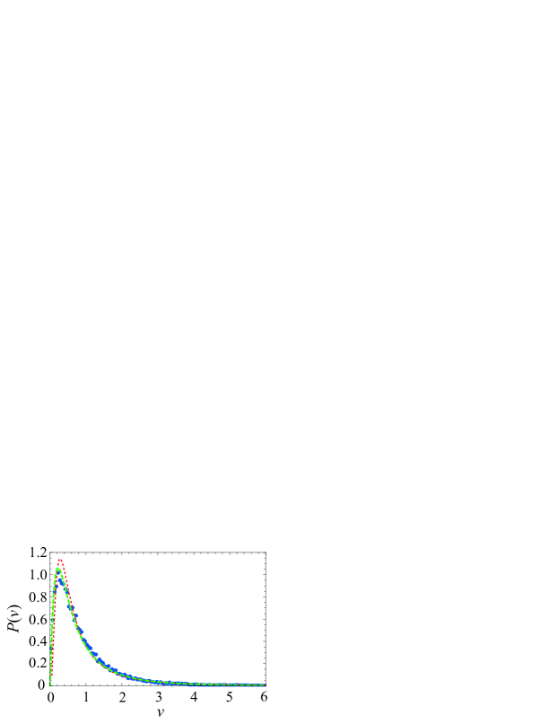
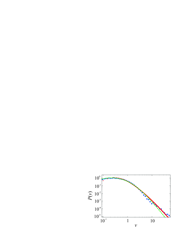
Figure 7: Long-term distribution function $P\left(v\right)$ vs $v$. The points the empirical PDF for the trading volumes of General Electric. The red dotted line is obtained by numerically integrating Eq. (2.2) assuming the approximations described in the text and the green dashed line was obtained using Eq. (22). The upper panel uses a $\log-\log$ scale and the lower panel uses a linear-linear scale.

2.3 Probing the relation between trading volume and price fluctuations at the mesoscopic scale

“It takes volume to make price move” karpoff . This assertion has been consistently quoted and used as the starting point of attempts to establish a dynamical relation between trading volume and price fluctuations volvol ; volvol2 ; scale . While the famous adage is strongly supported and cultivated by generations of brokers and econometricians, particularly those who are interested in futures futures , the evolution to a stronger quantitative approach based on high-frequency data analysis, especially the survey of order books, brought challenging explanations to the actual micro-mechanisms leading to the statistics of price fluctuations bfl , namely the fact that large fluctuations are the outcome of differences between ask and bid prices farmer . Nevertheless, the feeling that both plummets and significant increases are associated with large volumes remained, in part due to the fact that historical slumps (at the daily scale) were accompanied by large trading volumes and also because the cross-correlation function between price fluctuations and trading volume is above noise level. Therefore, the natural question is: what is the real impact of trading volume on price fluctuations? Since fat tails in the distribution of trading volume are mainly the outcome of the heterogeneities in the activity (in our case in $\phi$ and $\theta$) we can ask a slightly different question based on the classical works of Christie christie and Rogalsky rogalski : to what extent are price fluctuations determined by non-stationarity of the trading volume? From a probabilistic point of view, the simplest starting point to answer this question is to consider Bayes’ law,

$$\Pi\left(r\right)=\int p\left(r|v\right)P\left(v\right)dv.$$ (23)

For highly liquid blue chip companies and 1 minute sampling rate, we definitely have $P\left(v=0\right)=0$. Nonetheless, it is possible that a given volume $v$ yields no price fluctuation. To characterize the likelihood of this type of event, we defined a probability,

$$g^{\left(0\right)}\left(v\right)\equiv 1-g^{\left(+\right)}\left(v\right)-g^{\left(-\right)}\left(v\right),$$ (24)

where $g^{\left(\pm\right)}\left(v\right)$ corresponds to the probability of having a positive (negative) price fluctuation for a trading volume $v$. The functions $g^{\left(\pm\right)}\left(v\right)$ should verify two conditions: first, scraping events like stock splits and dividends, when there is no trading volume the price remains constant, i.e., $g(v^{(\pm)})(0)=0$; second, for large values of $v$, it most surely approaches a value independent of the trading volume, which is not necessarily equal for negative and positive price fluctuations, as verifiable in Fig. 8. For these reasons, we assumed that $g^{\left(\pm\right)}\left(v\right)$ is fairly described by,

$$g^{\left(\pm\right)}\left(v\right)=G\tanh\left(\varpi\ v^{\beta}\right).$$ (25)

Averaging over all the companies we have,

$$\begin{array}[]{cccc}&G&\varpi&\beta\vspace{0.15cm}\\ g^{\left(-\right)}:&0.4\pm 0.03&2.56\pm 0.87&0.3\pm 0.1\vspace{0.05cm}\\ g^{\left(+\right)}:&0.47\pm 0.04&1.22\pm 0.29&0.25\pm 0.05.\vspace{0.05cm}\end{array}$$

These values, followed by a visual inspection of Fig. 8, point that for small trading volume values the probability of having a negative value is higher than the probability of a positive value with the relation between $g^{\left(-\right)}$ and $g^{\left(-\right)}$ changing for $v\approx 1$. At first glance and taking into consideration the risk-aversion ethos of financial agents, we would expect precisely the opposite, i.e., small trading values dominating price rises and large trading values associated with price decreases. However, minding the covariance $\left\langle(r-\left\langle r\right\rangle)(v-\left\langle v\right\rangle)\right\rangle$, we understand that this behavior corresponds to a high-frequency verification of Ying’s findings ying about the existence of a correlation between price fluctuations and trading volume thus providing some quantitative support to the adage.

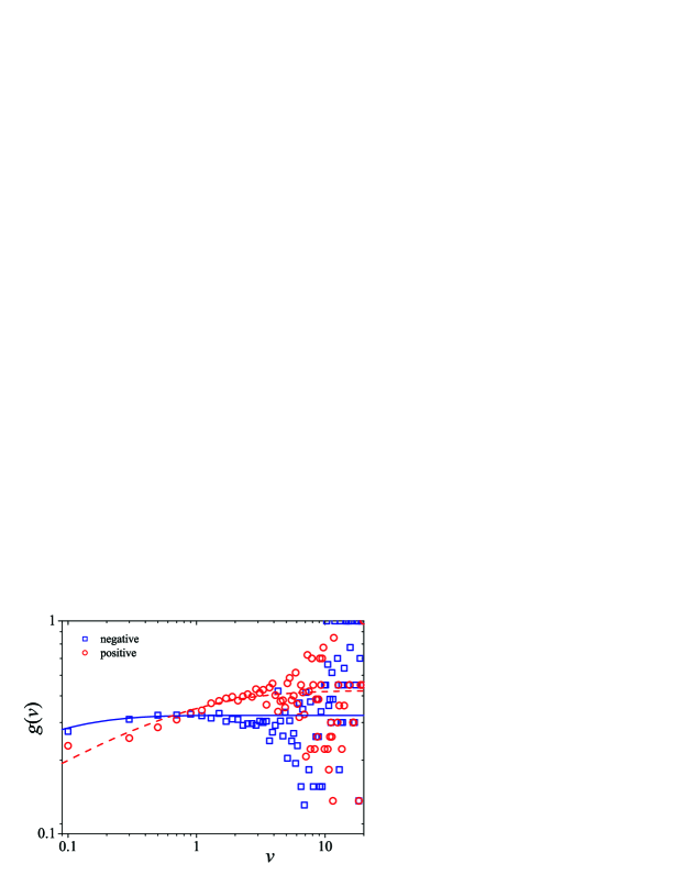
Figure 8: Probability of having a positive (negative) price fluctuation vs trading volume. The points were obtained for data of General Electric and the lines are the best fits using Eq. (25).

As regards trading volume associated with non-zero price fluctuations, it is worth appraising the relation between volume and the price fluctuations,

$$\begin{array}[]{c}\left|r_{t}\right|=\left\langle\ \left|r\right|\ |\ v_{t}\right\rangle+\eta_{t}\vspace{0.1cm}\\ =\mathcal{I}\left(v\right)+\eta,\end{array}$$ (26)

where $\left\langle\,\left|r\right|\,|\ v\right\rangle$ represents the expected magnitude of the price fluctuation produced by trading volume $v$. We have represented this deterministic part of the relation between the price fluctuations and volume by $\mathcal{I}\left(v\right)$ dubbing it trading impact. Although the term impact has been introduced in the context of order book analysis impact , it has been employed in longer spells in which accumulated (meta) orders are considered prx-impact . At odds with first proposals that assumed a linear relation between the price difference and trading volume kyle , $S^{\prime}-S=\lambda^{-1}\,v$ (with $\lambda$ being the market depth), later approaches backed up by empirical analysis have proposed that the long term $\mathcal{I}\left(v\right)$ is well described by either power-law, $\left|r_{t}\right|\sim v_{t}^{\alpha}$, or logarithmic, $\left|r_{t}\right|\sim\log v_{t}$, forms for the Paris and London stock markets in the tick-by-tick farmer ; impactfunction and 30 minute scales hopman .

In what follows, we tested the homogeneity of such proposals, i.e., we aimed at finding whether the changes in the local features of trading volume would impinge over its relation to the price fluctuation. We carried out this approach twofold: we tried to find a relation between the parameters describing the form of the trading impact function and the size of the segments. Along these lines, we have tested three different forms,

$$\begin{array}[]{cc}\mathrm{i)}&\mathcal{I}\left(v\right)=a+b\ln v_{t},\vspace{0.05cm}\\ \mathrm{ii)}&\ln\,\mathcal{I}\left(v\right)=a+b\ln v_{t},\vspace{0.05cm}\\ \mathrm{iii)}&\ln\,\mathcal{I}\left(v\right)=a+b\,v_{t},\vspace{0.05cm}\end{array}$$ (27)

where we have considered different versions of each one for positive and negative returns. The power-law and logarithmic test functions are inspired by the previous work on impact functions and the exponential, case iii) in Eq. (27), is introduced because in complex systems it is ubiquitous the emergence of power-laws from a mixture of exponential functionals with different characteristic parameters. Since scatter plots of the price fluctuations with respect to the trading volume are rather noisy at a local scale, we resorted once more to the loess regression technique to describe cleaner curves. Afterwards, we adjusted these curves using the expressions in Eq. (27) and compared the $\chi^{2}$ per degree of freedom values in order to appraise which of the forms is the best. The average values for negative and positive returns are the following,

$$\begin{array}[]{cccc}&\chi^{2}\,\,(\mathrm{negative})&&\chi^{2}\,\,(\mathrm{positive})\vspace{0.15cm}\\ \mathrm{i)}&4\times 10^{-4}\pm 0.002&&9\times 10^{-5}\pm 3\times 10^{-4}\vspace{0.05cm}\\ \mathrm{ii)}&0.006\pm 0.003&&0.006\pm 0.003\vspace{0.05cm}\\ \mathrm{iii)}&0.045\pm 0.033&&0.042\pm 0.017\vspace{0.05cm}\,.\end{array}$$

Setting our sights on the best approach (smaller $\chi^{2}$ values), i.e., the logarithmic fit in Eq. (27), we have for the negative returns $a=$ $0.056\pm 0.021$ and $b=0.0062\pm 0.004$ and for positive returns $a=0.054\pm 0.015$ and $b=0.0059\pm 0.002$. In other words, we have not found a significant difference between positive and negative price fluctuations in respect of the trading impact. In addition, further statistical analysis of $a$ and $b$ showed that their distributions are significantly peaked.

Keeping our focus on the heterogeneities of the data, we further analyzed whether there is a relation between the parameters $a$, $b$ and the size of the segments, $\ell$ (see Fig. 9). Considering the linear adjustment of $a\left(\ell\right)$ and $b\left(\ell\right)$ for positive and negative price fluctuations, we verified they hardly vary with the segment length yielding median slopes equal to $s_{a}=\left\{-4.6\times 10^{-6},-4.3\times 10^{-6}\right\}$ and $s_{b}=\left\{-7.7\times 10^{-7},2.8\times 10^{-6}\right\}$ with the same behavior verified using local regression. Bearing in mind the magnitude of these slopes we assert that the trading impact functions are homogeneous. These two findings are represented in Fig. 9.

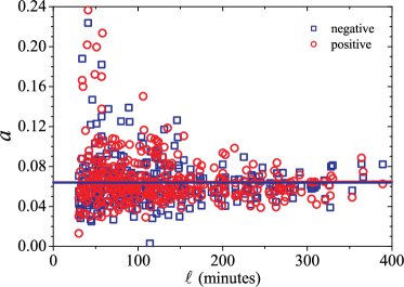
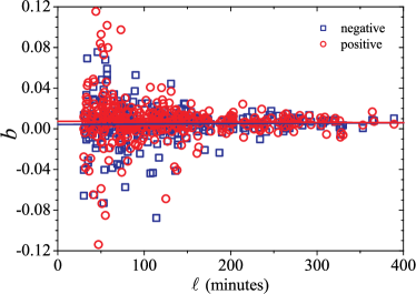
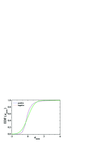
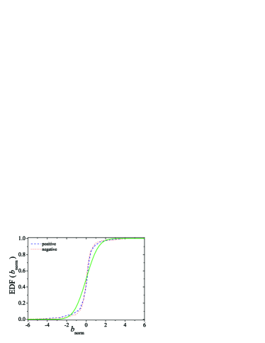
Figure 9: Left: value of parameter $a$ in test i) of Eq. (27) vs length of the segment $\ell$ (upper panel) and EDF of detrended and normalized $a$ (lower panel) for each patch. Right: the same but for parameter $b$. In the lower panels the green lines represent the complementary cumulative distribution function of the Normal distribution showing that both $a$ and $b$ are not Gaussian distributed in the long term. These data are for General Electric.

Let us finally introduce a simple argument which aims at explaining the expected relation between return and volume. First, we describe the simple case wherein a trading volume does not change the price. In this case, we have in the long-term,

$$\Pi\left(r=0\right)=\int\left[1-g^{\left(0\right)}\left(v\right)\right]\ P\left(v\right)\ dv,$$ (28)

where $P\left(v\right)$ is the long-term distribution Eq. (2.2) [or Eq. (22) in practical applications]. With respect to non-zero returns, the conditional distribution has got a different form, namely,

$$p\left(\,\left|r\right|\,|\ v\right)=f\left(\,\left|r\right|\,|\ v\right)\,\left(g^{\left(+\right)}\left(v\right)+g^{\left(-\right)}\left(v\right)\right),$$ (29)

where $f\left(\,\left|r\right|\,|\ v\right)$ is the double conditional probability of having a return of magnitude $\left|r\right|$ given a trading volume $v$ that produces a non-zero price fluctuation. Allowing for Eq. (26) and assuming that the error in the numerical adjustment, $\eta_{t}$, follows a Gaussian distribution,

$$\mathcal{G}(\eta;\left\{\left\langle\eta\right\rangle,\sigma_{\eta}\right\})=\frac{1}{\sqrt{2\,\pi}\,\sigma_{\eta}}\,\exp\left[-\frac{\left(\eta-\left\langle\eta\right\rangle\right)^{2}}{2\,\sigma_{\eta}^{2}}\right]$$ (30)

we have,

$$f\left(\left|r\right|\,|\ v\right)\approx\mathcal{G}\left(\left|r\right|;\left\{a+b\ln v,\sigma_{\eta}\right\}\right),$$ (31)

and thus finally for $\left|r\right|\neq 0$ we get,

$$\Pi\left(\left|r\right|\right)=\int\mathcal{N}_{r}\left(a+b\ln v,\sigma_{\eta}\right)\,\left(g^{\left(+\right)}\left(v\right)+g^{\left(-\right)}\left(v\right)\right)\,P\left(v\right)\,dv.$$ (32)

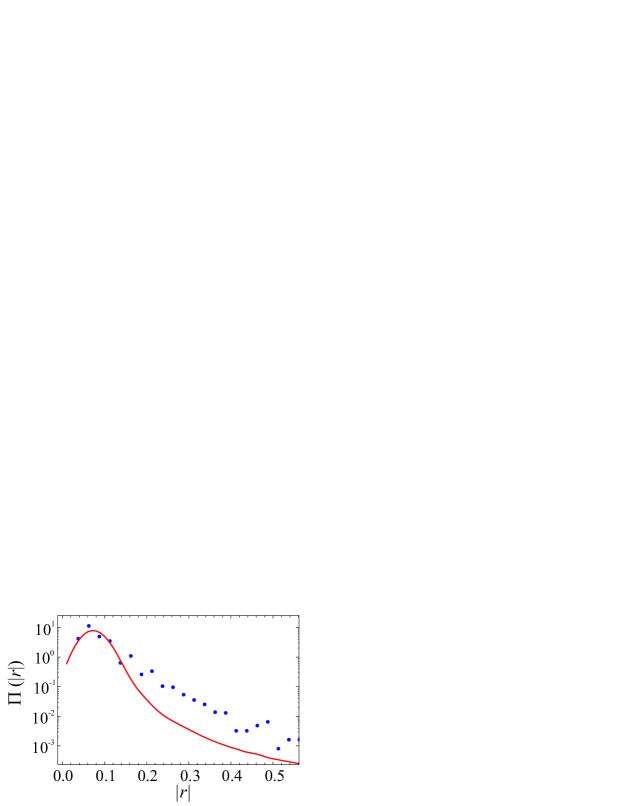
Figure 10: Probability of the magnitude of price fluctuations, $\Pi\left(\left|r\right|\right)$ , vs magnitude of the price fluctuations, $\left|r\right|$ for General Electric. The red line was obtained by the (numerical) integration of Eq. (32). The plot shows a factor 10 between data and the testing hypothesis.

Plugging Eq. (22) into Eq. (32), we are able to verify that although there is a relation between price fluctuations and trading volume, it only yields a fair representation of the peak of the distribution, which decays more slowly than the PDF from price – volume arguments (see Fig. 10). Taking into consideration that the peak of a distribution concentrates the key part of the measure, we can state that the heuristic adage relating trading volume and price fluctuations is in some sense verified. However, it completely fails at describing the stylized fact concerning the slow decay of the distribution $\Pi\left(\left|r\right|\right)$, as Fig. 10 clearly shows. So, what are the reasons for such misfire? Within the context of the heterogeneous approach, we can understand the different behavior of price fluctuations with respect to trading volume in applying the KSS algorithm. Looking at the results we present in Fig. 11, we found that the length of the segments of local stationarity in $|r|$ still follows a exponential like Eq. (2), but with a much short typical scale than the segmentation of trading volume, namely $\tau=77\pm 15$ minutes. This proves the different dynamics of both quantities, particularly the respective degree of non-stationarity. We still must remember that in the present approach, we wiped out factors like the fluctuations of the parameters of the local impact functions that can be regarded as a proxy for the local volatility. Accordingly, using a very different methodology our results go along the conclusion that large price fluctuations are more about the volatility than the volume scale ; farmer-bouchaud . We shall back to this point in the Discussion.

Figure 11: Cummulative distribution of the segments of the segmentation of the absolute values of the price fluctuations. Contrarily to Fig. 1, it is visible a clear exponential decay and the average over characteristic times yields $77\pm 15$ minutes. The qualitative behavior among stock is also different. In this case the less non-stationary series is United Technologies (UTX) whereas the most non-stationary is Pfizer (PFE).

3 Mixing description of price fluctuations

Having verified that trading volume is not a relevant factor leading to fat tails in the distribution of price fluctuations, we resort to the KSS in order to milk some further information on the impact of the non-stationarity of the returns in their local and long-term statistical properties. Traditionally, the volatility has been justified by the impact of trading orders, but recent results at the order book level as well as the results of our previous section have shown that volatility actually reflects a raft of other things, e.g., the random component in our trading impact among others. In our framework, the first thing to do is to classify the statistical nature of the local standard deviation. We assume as local volatility the variance of the corresponding segment resulting from the segmentation of the price fluctuations. Applying the same statistical procedures of Sec. 2.2, we verified that the best global distribution of the squared volatility (local variance) is given by the inverse-Gamma distribution of Eq. (8) with average parameters $\phi=2.5\pm 0.7$ and $\theta=(4\,\pm 1)\,\times 10^{-3}$. For some companies the Gamma distribution gave significant results as well. The observation of an inverse-Gamma distribution for the squared volatility is in accord with previous studies michiche but it concurs with previous theoretical approaches aimed at justifying the use of the Student-t (or $q$-Gaussian). However, this is just part of the story, to get such a long-term distribution we still need to give statistical evidence that the price fluctuations are locally Gaussian. Against the odds, we found that the local distribution is best locally described by an exponential distribution,

$$p(r;{\mu,\sigma})=\frac{1}{2\,\sigma}\,\exp\left[-\frac{|r-\mu|}{\sigma}\right],$$ (33)

for which the local average is equal to $\mu$ and the local variance is equal to $\Sigma\equiv 2\,\sigma^{2}$. Once again by employing the mixing indicated by Eq. (1) we obtain the long term distribution of the price fluctuations as presented in Fig. 12.

In place of looking for full integration, we can simplify the calculation of $P(r)$ noticing that the key deviation from the local exponential distribution comes from the large values of the volatility. When $\Sigma\rightarrow\infty$ its distribution decays as $\Sigma^{-1-\phi}$. Using the asymptotic behavior in the integration rather than its full form we get $P(r)\sim|r|^{-1-2\,\phi}$.

The plots in different types of scales clearly show that the local Gaussian distribution does not allow a good representation of the long-term distribution $P(r)$ both in the central part and the tails. In addition, we verified that $P(r)$ decays almost as an exponential, which is compatible with the large asymptotic exponent we obtained after using the values of $\phi$ found by fitting the local variance.

As a complement, we applied for each company the t-Student test numerical_recipes to verify whether the distributions of the local means of the returns were compatible with a zero mean normal distribution. The $p$-values obtained were $p<0.1$ for most companies; two companies with large $p$, namely Du Pont and McDonald’s have $p=0.39$ and $p=0.33$, respectively; and other five companies (Caterpillar, IBM, Johnson & Johnson, Altria and United Technologies) have $0.1<p<0.2$. Concerning the skewness and the kurtosis of the distributions, the Jarque-Bera jb test showed a very good agreement with a normal distribution, providing for all companies $p<0.001$.

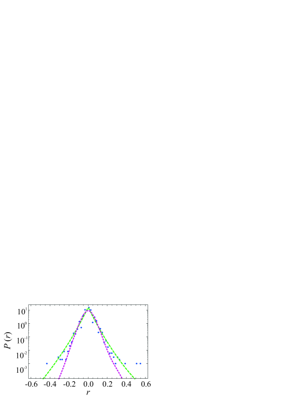
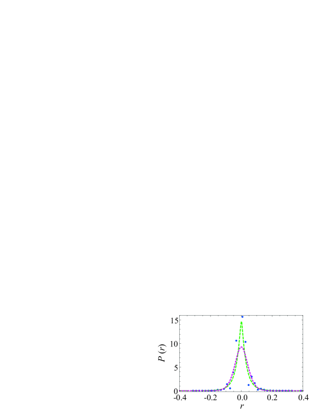
Figure 12: Long-term distribution of the price fluctuations in log-linear and linear-linear scales (upper and lower panels, respectively). The points correspond to the empirical PDF of General Electric. The green dashed line and the magenta dotted line are the long-term distribution obtained from the segmentation procedure considering an exponential and a Gaussian distribution. The parameters of the inverse-Gamma distribution of the squared volatility are $\phi=4.0$ and $\theta=6.3\times 10^{-3}$.

4 Discussion

In this work we inspected the effectiveness of the statistical mixture approach in mimicking primal financial quantities: price fluctuations and trading volume. We proved that the proper segmentation of the time series, which considers segments of varying length is fundamental for a correct description of statistical and dynamical stylized facts. We did it employing a non-parametric method of segmentation, the KSS kss , which assumes that differences between segments can derive from discrepancies in any statistical moment, which define the characteristic function of a probability density function.

Considering the trading volume, we reinforced the idea that a mixture of distributions is able to nicely describe its long term PDF. Specifically, from our results, the long-term PDF is effectually described by the statistical mixing of juxtaposed stationary segments of unequal length wherein the trading volume is log-Normal distributed. The distribution of the length of these segments is dominated by a exponential form with a typical scale around $115$ minutes, which decays much slowly for lengths greater than 330 minutes. This last regime mainly represents the behavior of patches of stationarity that last longer than a trading session. Bearing in mind stochastic mechanisms related to the log-normal distribution, we can think about this functional form of the trading volume as the result of a cascade of transactions, $v(i)=\prod_{\tau=1}^{n_{i}}T_{\tau}$, with $\ln T$ representing the log of the size of the $\tau$-th trade that is Gaussian distributed with average equal to $\mu$ and standard deviation equal t $\theta$.

Locally, we also verified that there is an intrinsic relation between the local average and the variance, i.e., between $\mu$ and $\theta$. With this relation, we were able to statistically express the local behavior in terms of a single local Log-Normal parameter [$\theta$ in Eq. (7)] that we learnt being well described by a Gamma distribution. In addition, we noted that segments with large local averages and small local averages behave differently and beyond statistical effects, albeit the description considering a single behavior also gives good results. These results are to be compared with the simpler approach of segments of constant length. At the probabilistic level, the former case gives a local distribution compatible with a Gamma distribution, which provides a fair local description of the data, with a $15\%$ handicap though. Notwithstanding, crucial differences arise in the description of the data: first, there is an important relation between the local average and variance that would not be learnt were we using fixed length segments or even applying a segmentation method based on the analysis of the means; Second, and most importantly, it would be impossible to capture and identify important dynamical stylized facts such as the U-shape of trading volume within each session; the slow decay of the autocorrelation function via the correlations of the average value of trading volume in juxtaposed stationary patches as well as the relation between the magnitude of the fluctuation of the segments length which are significantly correlated within the trading session span.

Stemming from such a good description of trading volume, we were able to shed light on the recent dispute between partisans of the famous relation between the trading volume and price fluctuations popularized by Karpoff in karpoff and new quantitative results that assign a minor role to volume in the dynamics of price fluctuations. Our results indicate that each assertion has its own domain of validity. On the one hand, we corroborated the claim conveyed in farmer ; impact that trading volume is not a key ingredient in large price fluctuations. On the other hand, holding on the statistical properties of trading volume we were capable of obtaining a fair representation of the central part of the distribution of the magnitude of price fluctuations. This finding agrees with the results of the cross-correlation between trading volume and price fluctuations volvol ; volvol2 ; ying , which are traditionally used as the main argument to defend the intimate relation between price and volume. However, our results clearly show that this cross-correlation (not greater than $20\%$) basically concentrates on small price fluctuations. Within our framework, the most straightforward explanation for the short-coming of the return — volume relation is given by the segmentation of the magnitude of the price fluctuations, the results of which are quite different from those we obtained for the trading volume. Explicitly, for the magnitude of price fluctuations we got a very clear exponential decay of the distribution of segments of local stationarity without the slower tail exhibited by the distribution trading volume segments. Quantitatively we found a typical scale around 75 minutes, which is substantially smaller than the 115 minutes found in the segmentation of trading volume. Since the length of the stationary segments acts as a simple, yet effective, way of quantifying the extension of the non-stationary nature of a time series, we can understand that changes in the impact of the volume or even in the probability of having non-zero price fluctuations occur at a faster scale that is not captured in the trading volume scale, leading to a faster decay of $\Pi(|r|)$. The effects we have just mentioned can be combined and represented by the volatility. Thence, working at a different scale our results prop up the statement that “there’s more to volatility than volume” farmer-bouchaud . Complementarily, we might also say that the adage about the volume being responsible for the price changes can be accepted in the same way Black-Scholes equation is valid in option pricing: it gives a fair forecast during a good part of the time, but it completely drops the clanger in the cases wherein one can make (lose) big money.

Finally, we verified that the (squared) volatility of price fluctuations evolves as an inverse-Gamma distribution, which perfectly tallies with the mixture distribution hypothesis that assumes price fluctuations are locally Gaussian distributed and which is the cornerstone of Engle’s ARCH model engle . Regardless, when we looked into the local distribution of price fluctuations we concluded that they do not follow a Gaussian distribution, but an exponential distribution instead. Were the local distribution Gaussian, we would have had a long term empirical distribution well described by a Student-t ($q$-Gaussian), which is not the case for both the central part and the tails. This result is interesting twofold: a) although the volatility process does not fit that of the Heston model heston , the local exponential we found agrees with the short term behavior of this model and b) It prompts the study of different definitions of noise in ARCH-like processes arches .

After bearing good fruit at the minute scale of stock trading, this method can be put to use in other financial problems at order book scale and enhance reasoning about other financial products. Concerning the former it would be interesting to analyze which additional features could be captured in the dynamical properties of individual agents previously studied by a comparison of the local means ibex . We should underscore that in the case of atmospheric turbulence kss , the test of the means is useless in the evaluation of local stationarity. In respect of other financial products, we can mention the dynamics of futures and other derivatives.

Appendix A KS-segmentation

Considering that a nonstationary time series can be split into stationary segments, the aim of segmentation is to find the optimal positions to separate the time series in such segments. In KSS, these positions are obtained by finding, along the series, the maximal

$$D\equiv D_{KS}(1/n_{L}+1/n_{R})^{-1/2},$$ (34)

where $n_{L}$ ($n_{R}$) is the number of points to the left (right) of the hypothetical cutting point and $D_{KS}$ is the Komogorov-Smirnov distance between the complementary cumulative distributions of these two samples. Once we find the position of maximal distance $D^{max}$, we test the statistical significance (at a chosen significance level $\alpha=1-P_{0}$) of a potentially relevant cut at that point. That is achieved by comparison with the value of $D$ that would be obtained was the sequence random. The critical value is given by the phenomenological expression kss

$$D^{max}_{crit}(n)=a(\ln n-b)^{c},$$ (35)

$(a,b,c)$ = ($1.41$, $1.74$, $0.15$), ($1.52$, $1.80$, $0.14$), and ($1.72$, $1.86$, $0.13$) for $P_{0}=0.90,0.95,0.99$, respectively. If $D^{max}$ exceeds the critical value for the selected significance level $D^{max}_{crit}(n)$, then the cut is done. The procedure is then recursively applied starting from the full series, until no segmentable patches are left. See kss for further details.

Appendix B Loess

In order to have a smooth set of points from scattered data $(x_{i},y_{i})$, $i=1,\dots,n$, we apply the robust locally weighted regression (loess) loess to obtain the estimated values for each point. The procedure consists of two parts. First, the weight function depends on the distance to the $r$-th nearest neighbor and a weighted least-squares fitting procedure gives the estimated values for each point. Second, a new factor is introduced in the weighting computation, based on the residuals of the first fitting procedure, improving the weights in the sense that large residuals will have small weights and small residuals will have large ones.

We can summarize the loess procedure as follows: for each point $i$, we compute the distance $h_{i}$ from $x_{i}$ to its $r$-th nearest neighbor. The $k=1,\dots,n$, (with $k\not=i$) weights for each point $x_{i}$ will be given by

$$\omega_{k}(x_{i})=W\left(\frac{x_{k}-x_{i}}{h_{i}}\right),$$ (36)

where $W$ is the tricubic weight function

$$W=\left\{\begin{array}[]{cc}(1-|x|^{3})^{3},&|x|<1\\[14.22636pt] 0,&|x|\geq 1.\\ \end{array}\right.$$

Then, in our cases, a linear least-squares fitting with weights given by Eq. (36) determines the estimated $\hat{y}_{i}$ that corresponds to $x_{i}$ and its residual, $e_{i}=y_{i}-\hat{y}_{i}$. A different set of weights, $\delta_{k}=W(e_{k}/(6\,s))$, is defined for each $(x_{i},y_{i})$ based on the size of $e_{i}$, and $s$ is the median of $|e_{i}|$. The new estimated values are obtained as before but with $\omega_{k}(x_{i})$ replaced by $\delta_{k}\omega_{k}(x_{i})$. This calculation of $\delta_{k}$ is iterated as much as necessary to have a satisfactory smoothed curve, for example when $s$ stabilizes. Further discussions and examples are presented in loess .

References

- (1) R.N. Mantegna and H.E. Stanley, An introduction to Econophysics: correlations and Complexity in Finance (Cambridge University Press, Cambrigde, 1999); J.-P. Bouchaud and M. Potters, Theory of Financial Risks: From Statistical Physics to Risk Management (Cambridge University Press, Cambridge, 2000); M. Dacorogna, R. Gençay, U. Müller, R. Olsen and O. Pictet, An Introduction to High-Frequency Finance (Academic Press, London, 2001) J. Voit, The Statistical Mechanics of Financial Markets (Springer-Verlag, Berlin, 2003)
- (2) W. Feller, An Introduction to Probability Theory and Its Applications Vol. 2 (John Wiley & Sons, New York, 1971)
- (3) T. Lux and M. Marchesi, Nature 397, 498 (1999); T. Lux and M. Marchesi, Int. J. Theor. Appl. Fin. 3, 675 (2000)
- (4) W. K. Bertram, Phys. A 341, 533 (2004)
- (5) E. Scalas, Chaos Sol. Frac. 34, 33 (2007)
- (6) M. Marsili, G. Raffaelli, B. Ponsot, J. Econ. Dyn. Cont. 33, 1170 (2009)
- (7) G. Livan, J. Inoue, E. Scalas, J. Stat. Mec. 12, 07025 (2012)
- (8) P. Gopikrishnan, V. Plerou, X. Gabaix and H.E. Stanley, Phys. Rev. E 62, R4493 (2000); R. Osorio, L. Borland and C. Tsallis, Distributions of High-Frequency Stock-Market Observablesin Nonextensive Entropy - Interdisciplinary Applications, 321-334, edited by M. Gell-Mann and C. Tsallis (Oxford University Press, New York, 2004); G.-H. Mu, W. Chen, J. Kertész and W.-X. Zhou, Eur. Phys. J. B 68, 145 (2009); G.-F. Gua, F. Rena, X.-H. Nia, W. Chene, W.-X. Zhou, Physica A 389, 278 (2010)
- (9) S.M. Duarte Queirós, Europhys. Lett. 71, 339 (2005)
- (10) A.A.G. Cortines, R. Riera and C. Anteneodo, EPL 83, 30003 (2008)
- (11) A. R. Gallant, P. E. Rossi, and G. Tauchen, Rev. Financ. Stud. 5, 199 (1992); C. Jones, K. Gautam and M.L. Lipson, Rev. Finan. Stud. 7, 631 (1994); X. Gabaix, P. Gopikrishnan, V. Plerou and H.E. Stanley, Nature 423, 267 (2003)
- (12) J.M. Karpoff, J. Finan. Quant. Anal. 22, 109 (1987)
- (13) E. Wienman, Principles of Multiscale Modeling (Cambridge University Press, Cambridge, 2011); J.-P. Fouque, G. Papanicolaou, R.Sircar, K, Sølna, Multiscale Stochastic Volatility for Equity, Interest Rate and Credit Derivatives (Cambridge University Press, Cambridge, 2011);
- (14) C. Beck, Phil. Trans. Royal Soc. A 369, 453 (2011); E. Van der Straeten and C. Beck, Phys. Rev. E 80, 036108 (2009)
- (15) C. Beck, E.G.D. Cohen, Phys. A 322, 267 (2003)
- (16) S. Camargo, S.M. Duarte Queirós and C. Anteneodo, Phys. Rev. E 84, 046702 (2011)
- (17) E. Moro, J. Vicente, L. G. Moyano, A. Gerig, J. Doyne Farmer, G. Vaglica, F. Lillo, R. N. Mantegna, Phys. Rev. E 80, 066102 (2009)
- (18) P. Bernaola-Galván, I. Grosse, P. Carpena, J. L. Oliver, R. Román-Roldán and H. E. Stanley, Phys. Rev. Lett. 85, 1342 (2000); W. Li, Phys. Rev. Lett. 86, 5815 (2001)
- (19) G. Shafer, J. Amer. Stat. Assoc. 77, 325 (1982); A. E. Raftery, Biometrika 83, 251 (1995)
- (20) B. Tóth, F. Lillo and J.D. Farmer, Eur. Phys. J. B 78, 235 (2010);
- (21) M.F.M. Osborne, Oper. Res. 7, 145 (1959); P.K. Clark, Econometrica 41, 135 (1973); G. Tauchen and M. Pitts, Econometrica 51, 485 (1983);
- (22) J. Ruseckas and B. Kaulakys, Phys. Rev. E 84, 051125 (2011); J. Ruseckas, V. Gontis and B. Kaulakys, Adv. Complex Syst. 15, 1250073 (2012)
- (23) J. de Souza, L.G. Moyano and S.M. Duarte Queirós, Eur. Phys. J. B 50, 165 (2006)
- (24) A. Admati and P. Pfleiderer, Rev. Financ. Stud. 1, 3 (1988); T. Andersen and T. Bollerslev, J. Empir. Financ. 4, 115 (1997); R. Allez and J.-P. Bouchaud, New J. Phys. 13, 025010 (2011)
- (25) C. Anteneodo and S.M. Duarte Queirós, J. Stat. Mech. P10023 (2010)
- (26) L.G. Moyano, J. de Souza and S.M. Duarte Queirós, Physica A 371, 118 (2006); Z. Eisler and J. Kertész, EPL 77, 28001 (2007)
- (27) A.R. Krommer and C.W. Ueberhuber, Computational Integration (SIAM Publications, Philadelphia, 1998)
- (28) C.W.J. Granger and O. Morgenstern, Kyklos 16, 1 (1963); C.M. Jones, G. Kaul and M.L. Lipson, Rev. Fin. Stud. 7, 631 (1994); K. Chan and W.-M. Fong, J. Fin. Econ. 57, 247 (2000) T.G. Andersen, J. Financ. 51, 169 (1996); H. Bessembinder and P.J. Seguin, J. Fin. Quantit. Anal. 28, 21 (1993)
- (29) T. Ané and L. Ureche-Rangau, Int. Fin. Markets, Inst. and Money 18, 216 (2008)
- (30) B. Cornell, J. Fut. Mark 1, 303 (1981); T.F. Martell and A.S.Wolf, J. Fut. Mark. 7, 233 (1987); R.T. Daigler and M.K. Wiley 54, J. Financ. 54, 2297 (1999); H.-G. Fung and G.A. Patterson, Int. Fin. Markets, Inst. and Money 9, 33 (2009);
- (31) J.-P. Bouchaud, J.D. Farmer and F. Lillo, How Markets Slowly Digest Changes in Supply and Demand, in Handbook of Financial Markets: Dynamics and Evolution, 57-156. edited by T. Hens and K. Schenk-Hoppe (Elsevier: Academic Press, New York, 2008).
- (32) J.D. Farmer and F. Lillo, Quantit. Financ. 4, 7 (2004); J.D. Farmer, L. Gillemot, F. Lillo, S. Mike and A. Sen, Quantit. Financ. 4, 383 (2004); P. Weber and B. Rosenow, Quantit. Financ. 6, 7 (2006)
- (33) A.A. Christie, On Information Arrival and Hypothesis Testing in Events Studies, University of Rochester Report number MERC/83-13 (1983) http://hdl.handle.net/1802/4856 [Last retrieved 7th August 2012]
- (34) R.J. Rogalski, Rev. Econ. Stat. 36, 268 (1978)
- (35) C.C. Ying, Econometrica 34, 676 (1966)
- (36) F. Lillo, J.D. Farmer and R.N. Mantegna, Nature 421, 129 (2003); J.D. Farmer, A. Gerig, F. Lillo and S. Mike, Quantit. Financ. 6, 107 (2006); J.D. Farmer and N. Zamani, Eur. Phys. J. B 55, 1899 (2007); P. Weber and B. Rosenow, Quantit. Financ. 5, 357 (2005); M. Wyart, J.-P. Bouchaud, J. Kockelkoren, M. Potters and M. Vettorazzo, Relation between bid-ask spread, impact and volatility in double auction markets. arXiv:physics/0603084v3 (preprint, 2006); W.-X. Zhou, New J. Phys. 14, 023055 (2012)
- (37) B. Tóth, Y. Lempérière, C. Deremble, J. de Lataillade, J. Kockelkoren and J.-P. Bouchaud, Phys. Rev. X 1, 021006 (2011)
- (38) A.S. Kyle, Econometrica 53, 1315 (1985)
- (39) M. Potters and J.-P. Bouchaud, Physica A 324, 133 (2003)
- (40) C. Hopman, Quantit. Financ. 7, 37 (2007)
- (41) L. Gillemot, J. D. Farmer, and F. Lillo, Quantit. Financ. 6, 371 (2006); S. Mike and J. Farmer, J. Econ. Dyn. and Control, 32, 200 (2008); A. Joulin, A. Lefevre, D. Grunberg and J.-P. Bouchaud, Stock price jumps: news and volume play a minor role. arXiv:0803.1769v1 (preprint, 2008)
- (42) Micciche et al. Physica A 314, 756761 (2002).
- (43) W. H. Press, Numerical Recipes in C, (Cambridge University Press, 1994)
- (44) C.M. Jarque and A.K. Bera, Econ. Lett. 6, 255 (1980).
- (45) R.F. Engle, Econometrica 50, 987 (1982)
- (46) S.L. Heston, Rev. Fin. Stud 6, 327 (1993); A.A. Drǎgulescu and V.M. Yakovenko, Quantit. Financ. 2, 443 (2002).
- (47) M. Porto and H.E. Roman, Phys. Rev. E 65, 046149 (2002); S.M. Duarte Queirós; C. Anteneodo and C. Tsallis, Power-law distributions in economics: a nonextensive statistical approach, in Noise and Fluctuations in Econophysics and Finance, Proc. of SPIE Vol. 5848, 151-164. edited by D. Abbott, J.P. Bouchaud, X. Gabaix and J.L. McCauley (SPIE, Bellingham -WA, 2005); T.G. Andersen, T. Bollerslev and F.X. Diebold, Parametric and Nonparametric Volatility Measurement, in Handbook of Financial Econometrics, 67-139. edited by Y. Aït-Sahalia and L.P. Hansen (Elsevier, Amsterdam, 2006)
- (48) G. Vaglica, F. Lillo, E. Moro and R.N. Mantegna, Phys. Rev. E 77, 036110 (2008)
- (49) W.S. Cleveland, J. Amer. Stat. Assoc. 74, 829 (1979); W.S. Cleveland and S.J. Devlin, J, Amer. Stat. Assoc. 83, 596 (1988)