Lattice BRST without Neuberger 0/0 problem

Abstract:

We illustrate in a simple toy model how the methods of SUSY quantum mechanics and topological quantum field theory can be used for covariant gauge-fixing with unbroken BRST symmetry on a finite lattice.

1 Introduction

The covariant continuum formulation of gauge theories in terms of local field systems relies on the existence of a well-defined and unbroken Becchi-Rouet-Stora-Tyutin (BRST) symmetry. In particular, the corresponding nilpotent BRST charge is needed to define the physical subspace of the indefinite metric state-space of covariant gauge theory in generalization of the Gupta-Bleuler condition in QED. This is all very well understood in perturbation theory. Beyond that, however, it is not so clear how to globally define such a BRST charge in presence of the inevitable Gribov copies. On the lattice, this problem is already present in the compact $U(1)$ gauge theory. Already there, there is a perfect cancellation of contributions from copies with even and odd numbers of negative eigenvalues of the Faddeev-Popov operator (i.e., even/odd Morse index) to the measure in a standard BRST formulation. This cancellation is the origin of the famous Neuberger $0/0$ problem of lattice BRST [1]. Thus, this problem needs to be solved in the compact $U(1)$ gauge theory already. The good news will be, however, that a solution to the Neuberger $0/0$ problem in compact $U(1)$, where it is a lattice artifact, is also suited for $SU(N)$ gauge theories with little extra work. It is simply applied to the maximal Abelian subgroup $U(1)^{N-1}$, the coset space $SU(N)/U(1)^{N-1}$ has no extra $0/0$ problem [2]. The corresponding lattice BRST for gauge fixing the $SU(2)/U(1)$ coset space was explicitly constructed already in Ref. [3].

After a short review of the standard procedure and its failure in the next section, we will walk through the $U(1)$ problem in more detail in a simple one-link model in Section 3. We explain the necessary extensions for $SU(2)$ in Section 4 and provide our summary and outlook in Sec. 5.

2 Standard (double) BRST on the lattice

The basic idea behind formulating (double) BRST on a finite lattice with the methods of SUSY quantum mechanics is to formulate a topological Witten model on the lattice gauge group whose partition function is to be used as the gauge-fixing device. BRST $s$ and anti-BRST $\bar{s}$ variations are thereby introduced as infinitesimal right multiplications of the $SU(N)$ gauge group elements $g$ by Lie-algebra valued, anti-Hermitian ghost and anti-ghost fields $c^{\dagger}=-c$ and $\bar{c}^{\dagger}=-\bar{c}$,

$$sg\,=\,g\,X^{a}c^{a}\,=\,gc\;,\qquad\bar{s}g\,=\,g\,X^{a}\bar{c}^{a}\,=\,g\bar{c}\;,$$ (1)

where $[X^{a},X^{b}]=f^{abc}X^{c}$ with $\mathrm{tr}\,X^{a}X^{b}=-\frac{1}{2}\delta^{ab}$. The partition function of this topological model must be independent of the link variables $U_{ij}$ connecting nearest neighbor sites $i\sim j$ which only enter via the gauge-fixing potential $V_{U}[g]$. In the standard case, for example,

$$V_{U}[g]=-\sum_{i,j\sim i}\mathrm{Re}\,\mathrm{tr}\,U_{ij}^{g}\;,\quad\mbox{where}\quad U_{ij}^{g}=g_{i}^{\dagger}U_{ij}g_{j}\;.$$ (2)

In terms of these, the BRST and anti-BRST transformations then take the more familiar form,

$$sU_{ij}^{g}=-c_{i}U_{ij}^{g}+U_{ij}^{g}c_{j}\;,\qquad\bar{s}U_{ij}^{g}=-\bar{c}_{i}U_{ij}^{g}+U_{ij}^{g}\bar{c}_{j}\;.$$ (3)

The (anti-)BRST transformations of ghost, anti-ghost and Nakanishi-Lautrup fields $b^{a}$ act per site and are the same as in the continuum [4],

$$\begin{array}[]{lll}sc^{a}=-\frac{1}{2}(c\times c)^{a}&&\bar{s}\bar{c}^{a}=-\frac{1}{2}(\bar{c}\times\bar{c})^{a}\\ s\bar{c}^{a}=b^{a}-\frac{1}{2}(\bar{c}\times c)^{a}&&\bar{s}c^{a}=-b^{a}-\frac{1}{2}(\bar{c}\times c)^{a}\\ sb^{a}=-\frac{1}{2}(c\times b)^{a}-\frac{1}{8}\big{(}(c\times c)\times\bar{c}\big{)}^{a}&&\bar{s}b^{a}=-\frac{1}{2}(\bar{c}\times b)^{a}+\frac{1}{8}\big{(}(\bar{c}\times\bar{c})\times c\big{)}^{a}\end{array}$$ (4)

where $(c\times c)^{a}\equiv f^{abc}c^{b}c^{c}$, etc. Ghost number and Faddeev-Popov conjugation are part of a global $SL(2,\mathbb{R})$ symmetry in this extended double BRST formulation with gauge-fixing action [5],

$$S_{\mathrm{gf}}\,=-i\,s\bar{s}\,\Big{(}V_{U}[g]+i\frac{\xi}{2}\sum_{i}\bar{c}_{i}c_{i}\Big{)}\,=\,\sum_{i}\Big{(}ib_{i}F_{i}[U^{g}]+i\bar{c}_{i}M_{i}[U^{g},c]+\frac{\xi}{2}b_{i}b_{i}+\frac{\xi}{8}(\bar{c}_{i}\times c_{i})^{2}\Big{)}\,.$$ (5)

Here we dropped the color indices for brevity. The Faddeev-Popov operator $M$ is the Hessian of the Morse potential $V_{U}[g]$, and as such it is Hermitian for all $\xi$. In Landau gauge, $\xi=0$, the $b$-fields establish $F_{i}[U^{g}]=0$ and the corresponding gauge-fixing partition function evaluates to

$$Z_{\mathrm{gf}}=\int d[g,b,\bar{c},c]\exp\{-S_{\mathrm{gf}}\}\stackrel{{\scriptstyle\xi=0}}{{=}}\sum_{\mathrm{copies}}\frac{\text{det}\,M_{F}}{|\text{det}\,M_{F}|}\,.$$ (6)

This is the sign-weighted sum over all Gribov copies whose vanishing causes the $0/0$ problem of lattice BRST upon inserting $Z_{\mathrm{gf}}$ into the unfixed partition function $Z=\int d[U]\exp\{-S[U]\}$ of the gauge theory on the lattice. To see this explicitly one introduces with Neuberger a parameter $t$,

$$S_{\mathrm{gf}}(t)\,=-i\,s\bar{s}\,\Big{(}\,t\,V_{U}[g]+i\frac{\xi}{2}\sum_{i}\bar{c}_{i}c_{i}\Big{)}\,,\quad\mbox{such that}\quad\frac{d}{dt}Z_{\mathrm{gf}}(t)=0\;,$$ (7)

just as $Z_{\mathrm{gf}}$ is independent of $\xi$ because both terms in the action are separately BRST exact. Moreover observing that $Z_{\mathrm{gf}}(t=0)=0$ then establishes the $0/0$ problem. The reason for this is that $Z_{\mathrm{gf}}$ computes the Euler characteristic $\chi$ of the lattice gauge group which is zero,

$$Z_{\mathrm{gf}}=\chi(SU(N)^{\times\#\mathrm{sites}})=\chi(SU(N))^{\#\mathrm{sites}},\quad\chi(SU(N))=\chi(S^{3})\chi(S^{5})\cdots\chi(S^{2N-1})=0\,,$$ (8)

because of the $N-1$ odd spheres that make up the group manifold. And just as this zero was obtained for $\xi=0$ in (6) via the Poincaré-Hopf theorem [6], here it follows from one Gauss-Bonnet integral expression for $\chi(SU(N))$ per site on the lattice [5],

$$Z_{\mathrm{gf}}(t=0)=\int d[g,b,\bar{c},c]\;\exp\Big{\{}-\sum_{i}\Big{(}\frac{\xi}{2}b_{i}b_{i}+\frac{\xi}{8}(\bar{c}_{i}\times c_{i})^{2}\Big{)}\Big{\}}\,.$$ (9)

One possible remedy is to introduce a Curci-Ferrari mass term [7] by replacing $S_{\mathrm{gf}}$ with

$$S_{\mathrm{mgf}}=-i\,(s\bar{s}+im^{2})\,\Big{(}\,t\,V_{U}[g]+i\frac{\xi}{2}\sum_{i}\bar{c}_{i}c_{i}\Big{)}\,.$$ (10)

This decontracts the extended double BRST algebra. BRST transformations are no-longer nilpotent, and the different Gribov copies get reweighted by the explicit BRST breaking proportional to the Curci-Ferrari mass parameter $m^{2}$. Instead of (6) in Landau gauge one then obtains

$$Z_{\mathrm{mgf}}\stackrel{{\scriptstyle\xi=0}}{{=}}\sum_{\mathrm{copies}}\text{sign}\big{(}\text{det}\,M_{F}\big{)}\,\exp\{-m^{2}tV_{U}[g]\}\,,$$ (11)

which lifts the cancellation of Gribov copies at the price of unitarity violations in the corresponding continuum theory at finite $m^{2}$. It also regulates the $t=0$ limit, e.g., explicitly for $SU(3)$ [5],

$$Z_{\mathrm{mgf}}(t=0)\propto(\xi m^{4})^{\#\mathrm{sites}}\Big{(}1+4\xi m^{4}+\frac{64}{15}(\xi m^{4})^{2}+\frac{64}{45}(\xi m^{4})^{3}\Big{)}^{\#\mathrm{sites}}\,,$$ (12)

and thus the $0/0$ problem. One might then hope to be able to restore unitarity and compute observables in limit $m^{2}\to 0$ from l’Hospital’s rule. Another way forward is to change the gauge-fixing potential. For $SU(2)$ for example it was suggested in [8, 9] to replace

$$V_{U}[g]=-\sum_{\mathrm{links}}\frac{1}{2}\text{tr}\,U^{g}\quad\text{by}\qquad\widetilde{V}_{U}[g]=-\sum_{\text{links}}\ln\big{(}1+\frac{1}{2}\text{tr}\,U^{g}\big{)}\,.$$ (13)

Near the identity they are essentially the same, so they are equivalent, perturbatively, and they both lead to the same continuum formulation. $\widetilde{V}_{U}$ is singular, however, whenever a gauge orbit passes through the south pole. This amounts to setting up a Witten model, but instead of $\chi(S^{3})=0$ for $SU(2)$ based on

$$\chi(\mathbb{R}P^{2})=\frac{1}{2}\,\chi(S^{2})=1\,,$$ (14)

for the $SU(2)/U(1)$ coset. The difference between the two lies in the way the diagonal $U(1)$ subgroup is treated. We discuss this in a toy-model next.

3 One-link model for compact $U(1)$

In order to illustrate the close connection to SUSY quantum mechanics we consider the simplest case of a single compact $U(1)$ degree of freedom $\varphi$ corresponding to a one-link model [10, 7]. In addition we use a single angle $\theta\in(-\pi,\pi]$ for a non-periodic gauge transformation $\varphi^{\theta}\equiv\varphi-\theta$ which we furthermore allow to depend on a fictitious time $\tau\in S^{1}$. With periodic boundary conditions for all gauge dof’s $\theta$, $b$ and Grassmann $\bar{c}$, $c$, we can then write down an action for the corresponding toy model in SUSY quantum mechanics [6],

$$S_{\mathrm{gf}}=\int_{0}^{1}d\tau\left[i\Big{(}\dot{\theta}+t\frac{\partial V_{\varphi}}{\partial\theta}\Big{)}b+\frac{\xi}{2}b^{2}+\bar{c}\Big{(}\frac{d}{d\tau}+t\frac{\partial^{2}V_{\varphi}}{\partial\theta^{2}}\Big{)}c\right]\,.$$ (15)

The corresponding partition function is independent of gauge parameters $t$, $\xi$ and link angle $\varphi$, and it is semiclassically exact. If the height function on the circle is used as the Morse potential, $V_{\varphi}(\theta)=1-\cos(\varphi-\theta)$ for the standard lattice Landau gauge, one thus readily confirms that

$$Z_{\mathrm{gf}}=\chi(S^{1})=\frac{1}{|t|}\,\big{(}t-t\big{)}=0\,.$$ (16)

The same will be true for any continuous periodic potential $V$ with isolated zeroes on the circle. The link angle is inessential here and will also be dropped in the following. We need to introduce a singularity in $V$ to allow odd numbers of critical points and thus avoid this topological obstruction. Before we proceed, we note that after redefining $t\to\xi t$ and then rescaling $\xi\tau\to\tau$,

$$S_{\mathrm{gf}}=\int_{0}^{\xi}d\tau\left[i\Big{(}\dot{\theta}+t\frac{\partial V}{\partial\theta}\Big{)}b+\frac{1}{2}b^{2}+\bar{c}\Big{(}\frac{d}{d\tau}+t\frac{\partial^{2}V}{\partial\theta^{2}}\Big{)}c\right]\,.$$ (17)

This form allows to identify Landau gauge as the “high temperature” limit $\xi\to 0$ of a Witten model in which all non-constant modes decouple, and in which the $\tau$-dependence is thus gone again. The gauge-fixing partition function is given by the path integral representation of the Witten index $\mathcal{W}=\Delta(\xi)$ of the model in heat-kernel regularization,

$$Z_{\mathrm{gf}}=\int\mathcal{D}[\theta,b,\bar{c},c]\,\exp\{-S_{\mathrm{gf}}\}=\Delta(\xi)=\text{Tr}\big{(}(-1)^{\mathcal{F}}e^{-\xi H}\big{)}=\text{Tr}\big{(}e^{-\xi H_{-}}\big{)}-\text{Tr}\big{(}e^{-\xi H_{+}}\big{)}\,.$$ (18)

Using $\bar{c}=c^{\dagger}$ for the Grassmann ghost in the operator language BRST and anti-BRST charges are identified with the ($N=2$) complex supercharges $Q$, $Q^{\dagger}$ and generalized ladder operators $A$, $A^{\dagger}$,

$$\begin{split}Q&=-\frac{i}{\sqrt{2}}bc^{\dagger}\equiv A\sigma_{+}=\frac{1}{\sqrt{2}}\left(\frac{d}{d\theta}+\Phi(\theta)\right)\sigma_{+}\,,\\ Q^{\dagger}&=\frac{i}{\sqrt{2}}b^{\dagger}c\equiv A^{\dagger}\sigma_{-}=\frac{1}{\sqrt{2}}\left(-\frac{d}{d\theta}+\Phi(\theta)\right)\sigma_{-}\,,\end{split}$$ (19)

of the Witten model with SUSY potential $\Phi(\theta)=tV^{\prime}(\theta)$ and partner Hamiltonians

$$H_{\pm}=\frac{p^{2}}{2}+\frac{1}{2}\Phi^{2}(\theta)\pm\frac{1}{2}\Phi^{\prime}(\theta)\equiv\frac{p^{2}}{2}+V_{\pm}(\theta)\,.$$ (20)

We can thus immediately write down the normalizable zero-energy ground state solutions to

$$\Big{(}\pm\frac{d}{d\theta}+\Phi(\theta)\Big{)}\,\phi_{0}^{\mp}(\theta)=0$$ (21)

on the finite interval $\theta\in[-\pi,\pi]$ with periodic boundary conditions $\phi(-\pi)=\phi(\pi)$. Whether the Witten index vanishes or not only depends on what we choose for the (pre)potential $V(\theta)$.

Standard lattice Landau gauge thus corresponds to $V(\theta)=1-\cos\theta$ with SUSY potential $\Phi(\theta)=t\sin\theta$, and isospectral partner Hamiltonians with potentials $V_{\pm}(\theta)=\frac{1}{2}(t^{2}\sin^{2}\theta\pm t\cos\theta)$. For any value of $t$ they each have a normalizable zero-energy ground state with wave function

$$\phi_{0}^{\pm}(\theta)=C\exp\{\pm t\cos\theta\}\,.$$ (22)

As before, the Witten index counting the number of bosonic minus fermionic ground states is zero, $\Delta=n_{-}-n_{+}=1-1=0$.

For the modified lattice Landau gauge, on the other hand, with $V(\theta)=-2\ln\big{(}(1+\cos\theta)/{2}\big{)}$, and SUSY potential $\Phi(\theta)=2t\tan(\theta/2)$, the partner potentials

$$V_{\pm}(\theta)=\frac{1}{8}\left(\frac{4t(4t\pm 1)}{\cos^{2}(\theta/{2})}-(4t)^{2}\right)$$ (23)

belong to the class of shape-invariant symmetric Pöschl-Teller potentials with good SUSY [11], $\Delta=1$, and a unique bosonic ground state with wave function

$$\phi_{0}^{-}(\theta)=C\big{(}\cos(\theta/2)\big{)}^{4|t|}\,.$$ (24)

The ground-state wave functions for both cases are sketched in Fig. 1. As long as the Witten index $\mathcal{W}=\Delta(\xi)=Z_{\mathrm{gf}}$ is non-zero, the corresponding SUSY on the gauge group cannot break, and we will thus be guaranteed to have a well-defined and unbroken BRST symmetry as well. The shape-invariant Pöschl-Teller oscillator for compact $U(1)$ has good SUSY, can be solved exactly and it is straightforwardly generalized to a one-dimensional chain.

                                   $\phi_{0}^{-}(\theta)$               $\phi_{0}^{+}(\theta)$                                        $\phi_{0}^{-}(\theta)$

                 

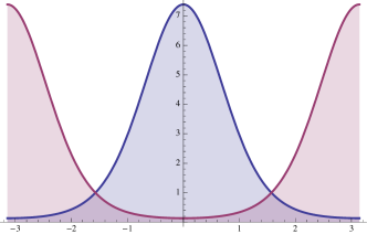
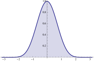
    $S$                        $N$                        $S$                   $S$                        $N$                        $S$

Figure 1: Ground-state wave functions for standard (left) and modified (right) gauge-fixing potentials in the one-link $U(1)$ model (15) with $t/\xi=2$. With the height function on the circle the bosonic ground state $\phi_{0}^{-}(\theta)$ centered around the North Pole at $\theta=0$ is always accompanied by a fermionic $\phi_{0}^{+}$ centered around the South Pole, $\theta=\pi$. In contrast, the Pöschl-Teller potential has a unique bosonic ground state.

Before we continue, it will be useful to write the $U(1)$ toy model in (15) in a manifestly coordinate and metric independent form [6]. For a general $z=f(\theta)$, the action in Eq. (15) becomes,

$$S_{\mathrm{gf}}=\int_{0}^{1}d\tau\left[i\big{(}\dot{z}g(z)+tV^{\prime}(z)\big{)}b+\frac{\xi}{2}g(z)b^{2}+\bar{c}\Big{(}g(z)D_{\tau}+t\big{(}V^{\prime\prime}(z)-\Gamma(z)V^{\prime}(z)\big{)}\Big{)}c\right]\,.$$ (25)

A particularly convenient coordinate is given by stereographically projecting the circle $S^{1}\to\mathbb{R}$ via $z=2\tan(\theta/2)$ for the modified potential $V(z)=2\ln(1+z^{2}/4)$, with one-dimensional metric

$$g(z)=\frac{1}{(1+z^{2}/4)^{2}}\,,\quad\Gamma=\frac{d}{dz}\ln\sqrt{g}=\frac{-z/2}{1+z^{2}/4}\,,$$ (26)

and covariant derivative $D_{\tau}=d/d\tau+\Gamma\dot{z}$. The fact that $Z_{\mathrm{gf}}=\mathcal{W}=1$, is then readily verified once more from the path integral representation (18) with the simple Nicolai map $\eta\equiv\dot{z}/(1+z^{2}/4)+tz$.

4 From compact $U(1)$ to $SU(2)$

Since we intend to use the supersymmetric Pöschl-Teller oscillator also for a $U(1)$ subgroup in $SU(2)$ we first focus on the two-dimensional coset $SU(2)/U(1)\simeq S^{2}$ (per site). The Euler characteristic of a two-dimensional compact manifold $\mathcal{M}$ is given by the integral over its Gauss curvature $K={R^{12}}_{12}$, the only independent component of the Riemann curvature tensor $R_{ijkl}$ in 2 dimensions,

$$\chi(\mathcal{M})=\frac{1}{2\pi}\int_{\mathcal{M}}K\,dv\,.$$ (27)

In particular, $K=1/R^{2}$ for a sphere $S_{R}^{2}$ of radius $R$, $dv=R^{2}d\Omega$ and the Euler characteristic is of course independent of $R$,

$$\chi(S_{R}^{2})=\chi(S^{2})=\frac{1}{2\pi}\int_{S^{2}}d\Omega=2\,.$$ (28)

A representation of this same Gauss-Bonnet formula which however holds for compact manifolds without boundary of any even dimension $2n$ involves $2n$ pairs of Grassmann variables $\bar{c}$, $c$, see [6],

$$\chi(\mathcal{M})=\int_{\mathcal{M}}d^{2n}x\int_{\mathbb{R}^{2n}}\frac{d^{2n}b}{(2\pi)^{2n}}\int d[\bar{c},c]\,\exp\left\{-\frac{\xi}{2}b^{i}b^{j}g_{ij}+\frac{\xi}{4}R_{ijkl}\bar{c}^{i}c^{k}\bar{c}^{j}c^{l}\right\}\,.$$ (29)

For odd-dimensional manifolds the corresponding result is automatically zero as it must because the exponential only produces even powers of the Grassmann variables. For the even-dimensional spheres $S_{R}^{2n}$ it is straightforward to verify that $\chi(S_{R}^{2n})=2$ from this formula. This can be done explicitly, e.g., with again using stereographic coordinates $\vec{x}\in\mathbb{R}^{2n}$ with $x=2R\tan(\theta/2)$, where $\theta$ is the azimuthal angle, metric $g_{ij}=(1+x^{2}/(2R)^{2})^{-2}\,\delta_{ij}$ and curvature $R_{ijkl}=R^{-2}(g_{ik}g_{jl}-g_{il}g_{jk})$.

For the projective space $\mathbb{R}P^{2}$ one either integrates only over one hemisphere to the equator at $x=2R$ or simply divides the full integral over $\vec{x}\in\mathbb{R}^{2}$ for $S^{2}$ by two as mentioned above. Since the Gauss-Bonnet integral for the Euler characteristic of a sphere is independent of its radius $R$ we may as well integrate $\chi(S_{R}^{2})$ over all $R$ with unit weight, $1=\int dR\,w(R)$, without changing the result, i.e., $\chi(S^{2})=\int dR\,\chi(S_{R}^{2})\,w(R)$. For this normalized integral we use the Witten index $\mathcal{W}=Z_{\mathrm{gf}}=1$ of the Pöschl-Teller oscillator with $S_{\mathrm{gf}}$ from (25) for $U(1)$ in the last section by identifying the radius $R$ of the two-sphere as $R=z=2\tan(\theta/2)$ where $\theta$ is now the azimuthal angle of $S^{3}$ for $SU(2)$.

What we have then achieved is to integrate in our final gauge-fixing partition function $Z_{\mathrm{gf}}$ for $SU(2)$ over the whole group manifold, however with $\theta\in(-\pi,\pi)$ in the Pöschl-Teller oscillator rather than $[0,\pi)$ for the usual azimuthal angle of $S^{3}$. The remaining two $S^{3}$ coordinates $\vec{x}$ then parametrize $\mathbb{R}P^{2}$ instead of $S^{2}$, hence we include a factor $1/2$ (per site). The partition function for the corresponding one-link model for $SU(2)$ then explicitly becomes

$$Z_{\mathrm{gf}}^{SU(2)}=\mbox{\small${\displaystyle\frac{1}{2}}$}\int\mathcal{D}[z,b_{z},\bar{c}_{z},c_{z}]\mathcal{D}[x,b_{x},\bar{c}_{x},c_{x}]\,\exp\{-S_{\mathrm{gf}}^{(x)}[x,b_{x},\bar{c}_{x},c_{x}]-S_{\mathrm{gf}}^{(z)}[z,b_{z},\bar{c}_{z},c_{z}]\}\,,$$ (30)

with $S_{\mathrm{gf}}^{(z)}[z,b,\bar{c},c]$ for the Pöschl-Teller oscillator as given in (25) and

$$S_{\mathrm{gf}}^{(x)}[x,b,\bar{c},c]=\int_{0}^{1}d\tau\,\Big{[}ig_{ij}\dot{x}^{i}b^{j}+\frac{\xi}{2}g_{ij}b^{i}b^{j}-\frac{\xi}{4}R_{ijkl}\bar{c}^{i}c^{k}\bar{c}^{j}c^{l}+\bar{c}^{i}g_{ij}(D_{\tau}c)^{j}\Big{]}\,,$$ (31)

with $i,j=1,2$. Since we did not need to introduce a Morse potential on $S^{2}$, the action in (31) is itself the $t\to 0$ limit of a Witten model to compute $\mathcal{W}=\chi(S^{2})$. In this limit, only the constant modes contribute and the path integral reduces to the corresponding Gauss-Bonnet integral (29). If we however now change coordinates from $z=2\tan(\theta/2)\in\mathbb{R}$, or $\theta\in(-\pi,\pi)$, and $\vec{x}\in\mathbb{R}P^{2}$ to general coordinates for $S^{3}$, the Pöschl-Teller prepotential $V(\theta)$, here defined as function of the class angle $\theta$ of $SU(2)$, will then depend on all three of the new coordinates. For example, with stereographic coordinates $\vec{x}\in\mathbb{R}^{3}$ with $x=2\tan(\theta/2)$ for $S^{3}$, the total gauge fixing action, the sum of $S_{\mathrm{gf}}^{(x)}$ and $S_{\mathrm{gf}}^{(z)}$, will be of the form

$$S_{\mathrm{gf}}^{(\mathrm{tot})} =\int_{0}^{1}d\tau\,\Big{[}i\Big{(}\dot{x}^{a}g_{ab}+t\frac{\partial V}{\partial x^{b}}\Big{)}b^{b}+\frac{\xi}{2}g_{ab}b^{a}b^{b}-\frac{\xi}{4}R_{abcd}\bar{c}^{a}c^{c}\bar{c}^{b}c^{d}$$ (32)

$$\hskip 113.81102pt+\bar{c}^{a}\Big{(}g_{ab}(D_{\tau}c)^{b}+t\Big{(}\frac{\partial^{2}V}{\partial x^{a}\partial x^{b}}-\Gamma^{c}_{ab}\frac{\partial V}{\partial x^{c}}\Big{)}c^{b}\Big{)}\Big{]}\,,$$

where now $a,b,c=1,2,3$. It is important to remember here, however, that the metric $g_{ab}$ is the transformed product metric for $S^{2}\times S^{1}$, an originally block-diagonal one consisting of a $2\times 2$ metric $g_{ij}$ for $S_{R}^{2}$ and a one-dimensional metric as in (26) for $S^{1}$. Analogously, the curvature tensor here is the correspondingly transformed $R_{ijkl}=R^{-2}(g_{ik}g_{jl}-g_{il}g_{jk})$ with $i,j=1,2$ for $S_{R}^{2}$. In particular, it is not the curvature of $S^{3}$ or $SU(2)$ as in (5) with $R_{abcd}=\frac{1}{2}\varepsilon_{abe}{\varepsilon^{e}}_{cd}$ which would produce the Neuberger zero for $t\to 0$ and with a bounded gauge-fixing potential $V$.

A rescaling of the time interval as in (17) but now from $\tau\in[0,1]$ to $\tau\in[0,t]$ with $\xi\to t\xi$ shows that also for $t\to 0$ only constant modes survive, likewise. With one such set of constant modes to be integrated per site $i$ on a lattice, where the only coupling of neighboring sites comes from the gauge-fixing potential, the covariant gauge-fixing action for $SU(2)$ without $0/0$ problem becomes,

$$S_{\mathrm{gf}}=\sum_{i}\Big{\{}i\frac{\partial V}{\partial x_{i}^{a}}b_{i}^{a}+\frac{\xi}{2}g_{ab}b_{i}^{a}b_{i}^{b}-\frac{\xi}{4}R_{abcd}\bar{c}_{i}^{a}c_{i}^{c}\bar{c}_{i}^{b}c_{i}^{d}\Big{\}}+\sum_{i,j}\bar{c}_{i}^{a}\Big{(}\frac{\partial^{2}V}{\partial x_{i}^{a}\partial x_{j}^{b}}-\delta_{ij}\Gamma^{c}_{ab}\frac{\partial V}{\partial x_{j}^{c}}\Big{)}c_{j}^{b}\,.$$ (33)

This is essentially of the same form as in (5). The only differences are in the $S^{2}\times S^{1}$ metric and curvature to be used here as discussed above, and the singular gauge-fixing potential with $V\equiv\widetilde{V}_{U}[g]$ from (13) in order to quantize one Pöschl-Teller oscillator for the $SU(2)$ class angle per site on the lattice so that the corresponding $Z_{\mathrm{gf}}=\chi(\mathbb{R}P^{2})^{\#\mathrm{sites}}=1$. The fact that the modified gauge-fixing potential must have a singularity thereby only means that contributions from a gauge orbit close to that singularity, for $\widetilde{V}_{U}[g]$ in (13) at $U^{g}=-1$, are exponentially suppressed.

5 Summary and Outlook

Starting from a simple one-link model, we have described explicitly how the problem of gauge-fixing on the lattice can be formulated in terms of the Witten index in SUSY quantum mechanics. All excited states of gauge and ghost degrees of freedom then cancel and the gauge-fixing partition function is determined entirely by the zero-energy ground states. Therefore, after gauge-fixing the contribution of each gauge orbit is represented by the difference of bosonic and fermionic ground states in the Witten model along this orbit. The BRST and anti-BRST symmetries then correspond to the $N=2$ supercharges of the Witten model, and as long as the Witten index is non-zero, one is guaranteed to have a good SUSY and thus a well-defined and unbroken BRST symmetry.

This is all verified explicitly in our one-link model for $U(1)$ and $SU(2)$. The generalization to a one-dimensional chain is straightforward. The Pöschl-Teller oscillators for compact $U(1)$ only have bosonic ground states in higher dimensions as well [8], there are thus no cancellations. Counting these bosonic ground states in more than one dimension is a challenging problem, however [12]. The generalization to $SU(N)$ is not entirely straightforward either and currently in progress.

This work was supported by the Helmholtz International Center for FAIR within the LOEWE program of the State of Hesse and the European Commission, FP7-PEOPLE-2009-RG No. 249203.