An Improved Integrality Gap for Asymmetric TSP Paths

Abstract

The Asymmetric Traveling Salesperson Path Problem (ATSPP) is one where, given an asymmetric metric space $(V,d)$ with specified vertices $s$ and $t$, the goal is to find an $s$-$t$ path of minimum length that passes through all the vertices in $V$.

This problem is closely related to the Asymmetric TSP (ATSP), which seeks to find a tour (instead of an $s$-$t$ path) visiting all the nodes: for ATSP, a $\rho$-approximation guarantee implies an $O(\rho)$-approximation for ATSPP. However, no such connection is known for the integrality gaps of the linear programming relaxations for these problems: the current-best approximation algorithm for ATSPP is $O(\log n/\log\log n)$, whereas the best bound on the integrality gap of the natural LP relaxation (the subtour elimination LP) for ATSPP is $O(\log n)$.

In this paper, we close this gap, and improve the current best bound on the integrality gap from $O(\log n)$ to $O(\log n/\log\log n)$. The resulting algorithm uses the structure of narrow $s$-$t$ cuts in the LP solution to construct a (random) tree spanning tree that can be cheaply augmented to contain an Eulerian $s$-$t$ walk.

We also build on a result of Oveis Gharan and Saberi and show a strong form of Goddyn’s conjecture about thin spanning trees implies the integrality gap of the subtour elimination LP relaxation for ATSPP is bounded by a constant. Finally, we give a simpler family of instances showing the integrality gap of this LP is at least $2$.

1 Introduction

In the Asymmetric Traveling Salesperson Path Problem (ATSPP), we are given an asymmetric metric space $(V,d)$ (i.e., one where the distances satisfy the triangle inequality, but potentially not the symmetry condition), and also specified source and sink vertices $s$ and $t$, and the goal is to find an $s$-$t$ Hamilton path of minimum length.

ATSPP is a close relative of Asymmetric TSP (ATSP), where the goal is to find a Hamilton tour instead of an $s$-$t$ path. For ATSP, the $\log_{2}n$-approximation of Frieze, Galbiati, and Maffioli [10] from 1982 was the best result known for more than two decades, until it was finally improved by constant factors in [4, 13, 9]. A breakthrough on this problem was an $O(\smash{\frac{\log n}{\log\log n}})$-approximation due to Asadpour, Goemans, M ‘ a dry, Oveis Gharan, and Saberi [2]; they also bounded the integrality gap of the subtour elimination linear programming relaxation for ATSP by the same factor.

Somewhat surprisingly, the study of ATSPP has been of a more recent vintage: the first approximation algorithms appeared only around 2005 [15, 6, 9]. It is easily seen that the ATSP reduces to ATSPP in an approximation-preserving fashion (by guessing two consecutive nodes on the tour). In the other direction, Feige and Singh [9] show that a $\rho$-approximation for ATSP implies an $O(\rho)$-approximation for ATSPP. Using the above-mentioned $O(\smash{\frac{\log n}{\log\log n}})$-approximation for ATSP [2], this implies an $O(\smash{\frac{\log n}{\log\log n}})$-approximation for ATSPP as well.

The subtour elimination linear program generalizes simply to ATSPP and is given in Section 2. However, prior to our work, the best integrality gap known for this LP for ATSPP was still $O(\log n)$ [11]. In this paper we show the following result.

Theorem 1.1.

The integrality gap of the subtour elimination linear program for ATSPP is $O(\smash{\frac{\log n}{\log\log n}})$.

We also explore the connection between integrality gaps for ATSPP and the so-called “thin trees conjecture”. In particular, if Goddyn’s conjecture regarding thin trees holds with strong-enough quantitative bounds then the integrality gap of the subtour elimination LP for ATSPP is bounded by a constant. The precise statement of the conjecture and of our result can be found in Section 5. This is analogous to a similar statement made by Oveis Gharan and Saberi regarding the integrality gap of the subtour elimination LP for ATSP [18].

Finally, we give a simple construction showing that the integrality gap of this LP is at least $2$; this example is simpler than previous known integrality gap instance showing the same lower bound, due to Charikar, Goemans, and Karloff [5].

Given the central nature of linear programs in approximation algorithms, it is useful to understand the integrality gaps for linear programming relaxations of optimization problems. Not only does this study give us a deeper understanding into the underlying problems, but upper bounds on the integrality gap of LPs are often useful in approximating related problems. For example, the polylogarithmic approximation guarantees in the work of Nagarajan and Ravi [16] for Directed Orienteering and Minimum Ratio Rooted Cycle, and those in the work of Bateni and Chuzhoy [3] for Directed $k$-Stroll and Directed $k$-Tour were all improved by a factor of $\log\log n$ following the improved bound of $O(\smash{\frac{\log n}{\log\log n}})$ on the integrality gap of the subtour LP relaxation for ATSP. We emphasize that these improvements required the integrality gap bound improvement for ATSP, not merely improved approximation guarantees.

1.1 Our Approach

Our approach to bound the integrality gap for ATSPP is similar to that for ATSP [2, 18], but with some crucial differences. To prove Theorem 1.1, we sample a random spanning tree in the underlying undirected multigraph and then augment the directed version of this tree to an integral circulation using Hoffman’s circulation theorem while ensuring the $t$-$s$ edge is only used once. The support of this circulation is weakly connected, so it can be used to obtain an Eulerian circuit with no greater cost. Deleting the $t$-$s$ edge from this walk results in a spanning $s$-$t$ walk.

However, the non-Eulerian nature of ATSPP makes it difficult to satisfy the cut requirements in Hoffman’s circulation theorem if we sample the spanning tree directly from the distribution given by the LP solution. It turns out that the problems come from the $s$-$t$ cuts $U$ that are nearly-tight: i.e., which satisfy $1<x^{*}(\partial^{+}(U))<1+\tau$ for some small constant $\tau$ — these give rise to problems when the sampled spanning tree includes more than one edge across this cut. Such problems also arise in the symmetric TSP paths case (studied in the recent papers of An, Kleinberg, and Shmoys [1] and Sebő [21]): their approach is again to take a random tree directly from the distribution given by the optimal LP solution, but in some cases they need to boost the narrow cuts, and they show that the loss due to this boosting is small.

In our case, the asymmetry in the problem means that boosting the narrow cuts might be prohibitively expensive. Hence, our idea is to preprocess the distribution given by the LP solution to tighten the narrow cuts, so that we never pick two edges from a narrow cut. Since the original LP solution lies in the spanning tree polytope, lowering the fractional value on some edges means we need to raise the fractional value on other edges. This would cause the costs to increase, and the technical heart of the paper is to ensure this can be done with a small increase in the cost.

Our approach for proving an $O(1)$ integrality gap bound under the thin trees conjecture is similarly inspired by related work for ATSP [18], but, again, we must be careful to ensure that the thin tree crosses each narrow cut exactly once. We do this by finding a cheap thin tree “between” narrow cuts (which we will prove are nested) and then chaining these thin together trees by selecting a single edge across each narrow cut. The resulting tree will have the desired thinness properties.

1.2 Other Related Work

The first non-trivial approximation for ATSPP was an $O(\sqrt{n})$-approximation by Lam and Newman [15]. This was improved to $O(\log n)$ by Chekuri and Pál [6], and the constant was further improved in [9]. The paper [9] also showed that a $\rho$-approximation algorithm for ATSP can be used to obtain an $O(\rho)$-approximation algorithm for ATSPP. All these results are combinatorial and do not bound integrality gap of ATSPP. A bound of $O(\sqrt{n})$ on the integrality gap of ATSPP was given by Nagarajan and Ravi [17], and was improved to $O(\log n)$ by Friggstad, Salavatipour and Svitkina [11]. Note that there is still no result known that relates the integrality gaps of subtour elimination relaxations for ATSP and ATSPP in a black-box fashion.

In the symmetric case (where the problems become TSPP and TSP respectively), constant factor approximations and integrality gaps have long been known. We do not survey the rich body of literature on TSP here, instead pointing the reader to, e.g., the recent paper on graphical TSP by Sebő and Vygen [22]. An exception is a result of An, Kleinberg, and Shmoys [1], who give an upper bound of $1.618$ on integrality gap of the LP relaxation for the TSPP problem; their algorithm also proceeds via studying the narrow $s$-$t$ cuts, and the connections to our work are discussed in Section 1.1. This bound on the integrality gap was subsequently improved to $1.6$ via a more refined analysis by Sebő [21].

1.3 Notation and Preliminaries

Given a directed graph $G=(V,A)$, and two disjoint sets $U,U^{\prime}\subseteq V$, let $\partial(U;U^{\prime})=A\cap(U\times U^{\prime})$. We use the standard shorthand that $\partial^{+}(U):=\partial(U;V\setminus U)$, and $\partial^{-}(U):=\partial(V\setminus U;U)$. When the set $U$ is a singleton (say $U=\{u\}$), we use $\partial^{+}(u)$ or $\partial^{-}(u)$ instead of $\partial^{+}(\{u\})$ or $\partial^{-}(\{u\})$. For undirected graph $H=(V,E)$, we use $\partial(U;U^{\prime})$ to denote edges crossing between $U$ and $U^{\prime}$, and $\partial(U)$ to denote the edges with exactly one endpoint in $U$ (which is the same as $\partial(V\setminus U))$. For any subset $U\subseteq V$ we let $A(U)$ denote $A\cap(U\times U)$, the set of arcs with both endpoints in $U$. If we are discussing subsets of arcs ${B}$ of $G$, we add subscripts to the $\partial$ notation to indicate we only consider those arcs crossing the cut that in are ${B}$. For example, $\partial_{{B}}^{+}(U)$ denotes $\partial^{+}(U)\cap{B}$ and so on. A collection of subsets of $V$, say $\pi$ is a partition if each element of $V$ occurs in exactly one part of $\pi$. Given a graph $G=(V,E)$ and a partition $\Pi$ of $V$, we let $\partial(\pi)$ to be the set of edges in $E$ which have endpoints in different sets of $\pi$.

For a digraph $G=(V,A)$, a set of arcs $B\subseteq A$ is weakly connected if the undirected version of $B$ forms a connected graph that spans all vertices in $V$.

For values $x_{a}\in{\mathbb{R}}$ for all $a\in A$, and a set of arcs $B\subseteq A$, we let $x(B)$ denote the sum $\sum_{a\in B}x_{a}$.

Given an undirected graph $H=(V,E)$ and a subset of edges $F\subseteq E$, we let $\chi_{F}\in\{0,1\}^{|E|}$ denote the characteristic vector $F$. The spanning tree polytope is the convex hull of $\{\chi_{T}\mid T\text{ spanning tree of }H\}$. See, e.g., [20, Chapter 50] for several equivalent linear programming formulations of this polytope. We sometimes abuse notation and call a set of directed arcs $T$ a tree if the undirected version of $T$ is a tree in the usual sense.

A directed metric graph on vertices $V$ has arcs $A=\{uv:u,v\in V,u\neq v\}$ where the non-negative arc costs satisfy the triangle inequality $c_{uv}+c_{vw}\geq c_{uw}$ for all $u,v,w\in V$. However, arcs $uv$ and $vu$ need not have the same cost. An instance of ATSPP is a directed metric graph along with distinguished vertices $s\neq t$.

2 The Rounding Algorithm

In this section, we give the linear programming relaxation for ATSPP, and show how to round a feasible solution $x$ to this LP to get a path of cost $O(\smash{\frac{\log n}{\log\log n}})$ times the cost of $x$. We then give the proof, with some of the details being deferred to the following sections.

Given a directed metric graph $G=(V,A)$ with arc costs $\{c_{a}\}_{a\in A}$, we use the following standard linear programming relaxation for ATSPP which is also known as the subtour elimination linear program.

$${\rm minimize}:\sum_{a\in A}c_{a}x_{a}$$ (ATSPP)

$${\rm s.t.}:~{}~{}x(\partial^{+}(s))=x(\partial^{-}(t)) =1$$ (1)

$$x(\partial^{-}(s))=x(\partial^{+}(t)) =0$$ (2)

$$x(\partial^{+}(v))=x(\partial^{-}(v)) =1 \forall~{}v\in V\setminus\{s,t\}$$ (3)

$$x(\partial^{+}(U)) \geq 1 \forall~{}\{s\}\subseteq U\subsetneq V$$ (4)

$$x_{a} \geq 0 \forall~{}a\in A$$

Constraints (4) can be separated over in polynomial time using standard min-cut algorithms, so this LP can be solved in polynomial time using the ellipsoid method. We begin by solving the above LP to obtain an optimal solution $x^{*}$. Consider the undirected (multi)graph $H=(V,E)$ obtained by removing the orientation of the arcs of $G$. That is, create precisely two edges between every two nodes $u,v\in V$ in $H$, one having cost $c_{uv}$ and the other having cost $c_{vu}$. (Hence, $|E|=|A|$.) For a point $w\in{\mathbb{R}}_{+}^{A}$, let $\kappa(w)$ denote the corresponding point in ${\mathbb{R}}_{+}^{E}$, and view $\kappa(w)$ as the “undirected” version of $w$.

We will use the following definition: An $s$-$t$ cut is a subset $U\subset V$ such that $\{s\}\subseteq U\subseteq V\setminus\{t\}$. The following fact will be used throughout the paper.

Claim 2.1.

Let $x^{*}$ be a feasible solution to LP (ATSPP). For any $s-t$ cut $U$, $x^{*}(\partial^{+}(U))-x^{*}(\partial^{-}(U))=1$. Also, $x(\partial^{+}(U))=x^{*}(\partial^{-}(U))$ for every nonempty $U\subseteq V\setminus\{s,t\}$.

Proof.

For any nonempty subset of vertices $U$ we have

$$x^{*}(\partial^{+}(U))-x^{*}(\partial^{-}(U)) = \left(\sum_{e\in\partial^{+}(U)}x^{*}_{e}-\sum_{e\in A(U)}x^{*}_{e}\right)-\left(\sum_{e\in\partial^{-}(U)}x^{*}_{e}-\sum_{e\in A(U)}x^{*}_{e}\right)$$

$$= \sum_{v\in U}x(\partial^{+}(v))-\sum_{v\in U}x(\partial^{-}(v)).$$

If $U$ is an $s-t$ cut, then the first sum in the last expression is $|U|$ and the second sum is $|U|-1$ by Constraints (1), (2), and (3). If $U\subseteq V\setminus\{s,t\}$, then both sums are equal to $|U|$ by Constraints (3). ∎

Definition 2.2 (Narrow cuts).

Let $\tau\geq 0$. An $s$-$t$ cut $U$ is $\tau$-narrow if $x^{*}(\partial^{+}(U))<1+\tau$ (or equivalently, $x^{*}(\partial^{-}(U))<\tau$).

The main technical lemma is the following:

Lemma 2.3.

For any $\tau\in[0,1/4]$, one can find, in polynomial-time, a vector $z\in[0,1]^{A}$ (over the directed arcs) such that:

1. its undirected version $\kappa(z)$ lies in the spanning tree polytope for $H$,

2. $z\leq\frac{1}{1-3\tau}\,x^{*}$ (where the inequality denotes component-wise dominance), and

3. $z(\partial^{+}(U))=1$ and $z(\partial^{-}(U))=0$ for every $\tau$-narrow $s$-$t$ cut $U$.

Before we prove the lemma (in Section 2.1), let us sketch how it will be useful to get a cheap ATSPP solution. Since $z$ (or more correctly, its undirected version $\kappa(z)$) lies in the spanning tree polytope, it can be represented as a convex combination of spanning trees. Using some recently-developed algorithms (e.g., those due to [2, 7]) one can choose a (random) spanning tree that crosses each cut only $O(\smash{\frac{\log n}{\log\log n}})$ times more than the LP solution. Finally, we can use $O(\smash{\frac{\log n}{\log\log n}})$ times the LP solution to patch this tree to get an $s$-$t$ path. Since the LP solution is “weak” on the narrow cuts and may contribute very little to this patching (at most $\tau$), it is crucial that by property (c) above, this tree will cross the narrow cuts only once, and that too, it crosses in the “right” direction, so we never need to use the LP when verifying the cut conditions of Hoffman’s circulation theorem on narrow cuts. The details of these operations appear in Section 3.

We will assume $n\geq 7$ to ensure all of our arguments work. For $n\leq 6$, we use the known integrality gap bound of $2\lfloor\log_{2}n\rfloor+1\leq 5$ from [11] to ensure the gap is bounded for all $n\geq 2$.

2.1 The Structure of Narrow Cuts

We now prove Lemma 2.3: it says that we can take the LP solution $x^{*}$ and find another vector $z$ such that if an $s$-$t$ cut is narrow in $x^{*}$ (i.e. $x^{*}(\partial^{+}(U))<1+\tau$), then $z(\partial^{+}(U))=1$. Moreover, the undirected version of $z$ can be written as a convex combination of spanning trees, and $z_{a}$ is not much larger than $x^{*}_{a}$ for any arc $a$.

The undirected version of $x^{*}$ itself can be written as a convex combination of spanning trees, so if we force $z$ to cross the narrow cuts to an extent less than $x^{*}$ (loosely, this reduces the connectivity), we had better increase the value on other arcs. To show we can perform this operation without changing any of the coordinates by very much, we need to study the structure of narrow cuts more closely. (Such a study is done in the symmetric TSP path paper of An et al. [1], but our goals and theorems are somewhat different.)

First, say two $s$-$t$ cuts $U$ and $W$ cross if $U\setminus W$ and $W\setminus U$ are non-empty.

Lemma 2.4.

For $\tau\leq 1/4$, no two $\tau$-narrow $s$-$t$ cuts cross.

Proof.

Suppose $U$ and $W$ are crossing $\tau$-narrow $s$-$t$ cuts. Then

$$2+2\tau > x^{*}(\partial^{+}(U))+x^{*}(\partial^{+}(W))$$

$$= x^{*}(\partial^{+}(U\setminus W))+x^{*}(\partial^{+}(W\setminus U))+x^{*}(\partial^{+}(U\cap W))$$

$$+x^{*}(\partial(U\cap W;V\setminus(U\cup W)))-x^{*}(\partial((U\cup W)\setminus(U\cap W);U\cap W))$$

$$\geq 1+1+1+0-2\tau$$

$$= 3-2\tau$$

where the last inequality follows from the first three terms being cuts excluding $t$ and hence having at least unit $x^{*}$-value crossing them (by the LP constraints), the fourth term being non-negative, and the last term being the $x^{*}$-value of a subset of the arcs in $\partial^{-}(U)\cup\partial^{-}(W)$ and remembering that $U$ and $W$ are $\tau$-narrow. However, this contradicts $\tau\leq 1/4$. ∎

Lemma 2.4 says that the $\tau$-narrow cuts form a chain $\{s\}=U_{1}\subset U_{2}\subset\ldots\subset U_{k}=V\setminus\{t\}$ with $k\geq 2$. For $1<i\leq k$. let $L_{i}:=U_{i}\setminus U_{i-1}$. We also define $L_{1}=\{s\}$ and $L_{k+1}=\{t\}$. Let $L_{\leq i}:=\bigcup_{j=1}^{i}L_{i}$ and $L_{\geq i}:=\bigcup_{j=i}^{k+1}L_{i}$. For the rest of this paper, we will use $\tau$ to denote a value in the range $[0,1/4]$. Ultimately, we will set $\tau:=1/4$ for the final bound but we state the lemmas in their full generality for $\tau\leq 1/4$.

Next, we show that out of the (at most) $1+\tau$ mass of $x^{*}$ across each $\tau$-narrow cut $U_{i}$, most of it comes from the “local” arcs in $\partial(L_{i};L_{i+1})$.

Lemma 2.5.

For each $1\leq i\leq k$; $x^{*}(\partial(L_{i};L_{i+1}))\geq 1-3\tau$.

Proof.

If $k=1$ then $\{s\}=U_{1}=U_{k}=V\setminus\{t\}$ so in fact $V=\{s,t\}$. In this case, $L_{1}=\{s\}$ and $L_{2}=\{t\}$ and the LP constraints clearly imply $\partial(L_{1};L_{2})=1$.

Now consider the case $k\geq 2$. For $i=1$, since $s,t\not\in L_{2}$ we have $x^{*}(\partial^{-}(L_{2}))\geq 1$ from the LP constraints. We also have $x^{*}(\partial^{-}(U_{2}))<\tau$ because $U_{2}$ is $\tau$-narrow, and therefore $x^{*}(\partial(L_{1};L_{2}))\geq 1-\tau$. A similar argument for $i=k$ shows $x^{*}(\partial(L_{k};L_{k+1}))\geq 1-\tau$. So it remains to consider $1<i<k$. Define the following quantities, some of which can be zero.

• $A=x^{*}(\partial(L_{i};L_{i+1}))$

• $B=x^{*}(\partial(L_{i};L_{\geq i+2}))$

• $C=x^{*}(\partial(L_{\leq i-1};L_{i+1}))$

We have

$$1\leq x^{*}(\partial^{+}(L_{i}))=A+B+x^{*}(\partial(L_{i};L_{\leq i-1}))\leq A+B+\tau,$$

because $\partial(L_{i};L_{\leq i-1})\subseteq\partial^{-}(U_{i-1})$ and $U_{i-1}$ is $\tau$-narrow. Similarly

$$1\leq x^{*}(\partial^{-}(L_{i+1}))=A+C+x^{*}(\partial(L_{\geq i+2};L_{i+1}))\leq A+C+\tau.$$

Summing these two inequalities yields $2\leq A+(A+B+C)+2\tau\leq A+(1+\tau)+2\tau$ where we have used $A+B+C\leq x^{*}(\partial^{+}(U_{i}))\leq 1+\tau$. Rearranging shows $A\geq 1-3\tau$. ∎

Now, recall that $\kappa(x^{*})$ denotes the assignment of arc weights to the graph $H=(V,E)$ from the previous section obtained by “removing” the directions from arcs in $A$. We prove that the restriction of $\kappa(x^{*})$ to any $L_{i}$ almost satisfies the partition inequalities that characterize the convex hull of connected spanning subgraphs of $H$. This characterization was given by Edmonds [8]; see also Chapter 50, Corollary 50.8(a) in Schrijver [20]. We state it here for completeness.

Theorem 2.6.

[8] Let $G=(V,E)$ be a graph. Then the convex hull of all connected spanning subgraphs of $G$ is given by ${\mathcal{C}}(G)=\{x\in{\mathbb{R}}^{E}:x(\partial(\pi))\geq|\pi|-1\;\;\;\forall\textrm{ partitions }\pi\textrm{ of }V,\;\;0\leq x\leq 1\}$. Moreover, the convex hull of spanning trees of $G$ is given by ${\mathcal{C}}(G)\cap\{x\in{\mathbb{R}}^{E}:\sum_{e\in E}x_{e}=|V|-1\}$.

For a partition $\pi=\{W_{1},\ldots,W_{\ell}\}$ of a subset of $V$, we let $\partial(\pi)$ denote the set of edges whose endpoints lie in two different sets in the partition. To be clear, $\partial(\pi)$ does not contain any edge that has at least one endpoint in $V-\cup_{i=1}^{\ell}W_{i}$.

Lemma 2.7.

For any $1\leq i\leq k+1$ and any partition $\pi=\{W_{1},\ldots,W_{\ell}\}$ of $L_{i}$, we have $\kappa(x^{*})(\partial(\pi))\geq\ell-1-2\tau$.

Proof.

Since $L_{1}=\{s\}$ and $L_{k+1}=\{t\}$, there is nothing to prove for $i=1$ or $i=k+1$. So, we suppose $1<i<k+1$.

Consider the quantity $\alpha=\sum_{j=1}^{\ell}x^{*}(\partial^{+}(W_{j}))+x^{*}(\partial^{-}(W_{j}))$. On one hand $x^{*}(\partial^{+}(W_{j}))=x^{*}(\partial^{-}(W_{j}))\geq 1$ because neither $s$ nor $t$ lie in $W_{j}$ for any $1\leq j\leq\ell$, so $\alpha\geq 2\ell$. On the other hand, $\alpha$ counts each arc between two parts in $\pi$ exactly twice and each arc with one end in $L_{i}$ and the other not in $L_{i}$ precisely once. So, $\alpha=2\kappa(x^{*})(\partial(\pi))+x^{*}(\partial^{+}(L_{i}))+x^{*}(\partial^{-}(L_{i}))$.

Notice that $\partial^{+}(L_{i})$ and $\partial^{-}(L_{i})$ are disjoint subsets of $\partial^{+}(U_{i-1})\cup\partial^{-}(U_{i-1})\cup\partial^{+}(U_{i})\cup\partial^{-}(U_{i})$. So, since both $U_{i-1}$ and $U_{i}$ are $\tau$-narrow, $x(\partial^{+}(L_{i}))+x(\partial^{-}(L_{i}))<2+4\tau$. This shows $2\ell\leq\alpha<2\kappa(x^{*})(\partial(\pi))+2+4\tau$ which, after rearranging, is what we wanted to show. ∎

Corollary 2.8.

For any partition $\pi$ of $L_{i}$, we have $\frac{\kappa(x^{*})(\partial(\pi))}{1-2\tau}\geq|\pi|-1$.

Proof.

From Lemma 2.7, we have $\frac{\kappa(x^{*})(\partial(\pi))}{1-2\tau}\geq\frac{|\pi|-1-2\tau}{1-2\tau}\geq|\pi|-1$ for any $|\pi|\geq 2$. ∎

Finally, to efficiently implement the arguments in the proof of Lemma 2.3, we need to be able to efficiently find all $\tau$-narrow cuts $U_{i}$. This is done by a standard recursive algorithm that exploits the fact that the cuts are nested.

Lemma 2.9.

There is a polynomial-time algorithm to find all $\tau$-narrow $s-t$ cuts.

Proof.

Consider following recursive algorithm. As input, the routine is given a directed graph $H=(V^{\prime},A^{\prime})$ with arc weights $x^{*}_{a}$ and distinct nodes $s^{\prime},t^{\prime}$ where both $\{s^{\prime}\}$ and $V^{\prime}\setminus\{t^{\prime}\}$ are $\tau$-narrow. Say a $\tau$-narrow cut $U$ in $H$ is non-trivial if $U\neq\{s^{\prime}\}$ and $U\neq V^{\prime}\setminus\{t^{\prime}\}$. The claim is that the procedure will find all non-trivial $\tau$-narrow $s-t$ cuts of $H$, provided that they are nested.

The procedure works as follows. If there are non-trivial $\tau$-narrow $s-t$ cuts in $H$, then there are nodes $u,v\in V^{\prime}\setminus\{s^{\prime},t^{\prime}\}$ such that some $\tau$-narrow $s^{\prime}-t^{\prime}$ cut $U$ has $\{s^{\prime},u\}\subseteq U\subseteq V^{\prime}\setminus\{t^{\prime},v\}$. So, the procedure tries all $O(|V^{\prime}|^{2})$ pairs of distinct nodes $u,v$, contracts both $\{s^{\prime},u\}$ and $\{t^{\prime},v\}$ to a single node and determines if the minimum cut separating these contracted nodes has $x^{*}$-capacity less than $1+\tau$. If such a cut $U$ was found for some $u,v$, the algorithm makes two recursive calls, one with the contracted graph $H[V^{\prime}/U]$ with start node being the contraction of $U$ and end node being $t^{\prime}$, and the other with the contracted graph $H[V^{\prime}/(V^{\prime}\setminus U)]$ with start node $s^{\prime}$ and end node being the contraction of $V^{\prime}\setminus U$. After both recursive calls complete, the algorithm returns all $\tau$-narrow cuts found by these two recursive calls (of course, after expanding the contracted nodes) and the $\tau$-narrow cut $U$ itself. If such a cut $U$ was not found over all choices of $u,v$, then the algorithm returns nothing because there are no non-trivial $\tau$-narrow $s^{\prime}-t^{\prime}$ cuts in $H$.

It is easy to see that a non-trivial $\tau$-narrow cut in either contracted graph corresponds to a $\tau$-narrow cut in $H$. On the other hand, if the $\tau$-narrow $s^{\prime}-t^{\prime}$ cuts are nested in $H$, then every non-trivial $\tau$-narrow $s^{\prime}-t^{\prime}$ cut apart from $U$ itself corresponds to a non-trivial $\tau$-narrow cut in exactly one of $H[V^{\prime}/U]$ or $H[V^{\prime}/(V^{\prime}\setminus U)]$. Also, the $\tau$-narrow cuts in both contracted graphs remain nested. So, the recursive procedure finds all non-trivial $\tau$-narrow cuts of $H$. The number of recursive calls is at most the number of non-trivial $\tau$-narrow cuts, and this is at most $|V^{\prime}|$ because the cuts are nested so it is an efficient algorithm. We call this algorithm initially with graph $G$, start node $s$ and end node $t$. Lemma 2.4 implies the $\tau$-narrow $s-t$ cuts of $G$ are nested so the recursive procedure finds all non-trivial $\tau$-narrow cuts of $G$. Adding these to $\{s\}$ and $V\setminus\{t\}$ gives all $\tau$-narrow cuts of $G$. ∎

Proof of Lemma 2.3.

The claimed vector $z$ can be described by linear constraints: indeed, consider the following polytope on the variables $z$.

$$\kappa(z)(\partial(\pi)) \geq|\pi|-1 \forall{\rm~{}partitions~{}}\pi{\rm~{}of~{}}V$$ (5)

$$\sum_{a}z_{a} =n-1$$ (6)

$$z_{a} \leq{\textstyle\frac{1}{1-3\tau}}\,x^{*}_{a} \forall~{}a\in A$$ (7)

$$z(\partial^{+}(U_{i})) =1 \forall~{}\tau\text{-narrow~{}}\text{$s$-$t$}{\rm~{}cuts~{}}U_{i}$$ (8)

$$z(\partial^{-}(U_{i})) =0 \forall~{}\tau\text{-narrow~{}}\text{$s$-$t$}{\rm~{}cuts~{}}U_{i}$$ (9)

$$z_{a} \geq 0 \forall~{}a\in A$$ (10)

Consider the vector $z$ given as follows.

$$z_{a}=\begin{cases}\frac{x_{a}^{*}}{x^{*}(\partial(L_{i};L_{i+1}))}&\text{if $a\in\partial(L_{i};L_{i+1})$ for some $i$;}\\ \frac{x_{a}^{*}}{1-2\tau}&\text{if $a\in A(L_{i})$ for some $i$;}\\ 0&\text{otherwise.}\end{cases}$$ (11)

Constraints (9) and (10) are satisfied by construction. Constraint (7) follows from Lemma 2.5 for edges in $\partial(L_{i};L_{i+1})$ and by construction for rest of the edges. For constraint (8), note that

$$z(\partial^{+}(U_{i}))=z(\partial(L_{i};L_{i+1}))+z(\partial^{+}(U_{i})\setminus\partial(L_{i};L_{i+1}))=\frac{x^{*}(\partial(L_{i};L_{i+1}))}{x^{*}(\partial(L_{i};L_{i+1}))}+0=1.$$

Next we show Constraints (5) holds. It suffices to show that $\kappa(z)$ can be decomposed as a convex combination of characteristic vectors of connected graphs. For $1\leq i\leq k+1$, let $z^{i}$ denote the restriction of $\kappa(z)$ to edges whose endpoints are both contained in $L_{i}$. Then Corollary 2.8, Constraints (10), and [20, Corollary 50.8a] imply that $z^{i}$ can be decomposed as a convex combination of integral vectors, each of which corresponds to an edge set that is connected on $L_{i}$. Next, let $z^{\prime}$ denote the restriction of $\kappa(z)$ to edges whose endpoints are both contained in some common $L_{i}$. Since the sets $E(L_{1}),\ldots,E(L_{k+1})$ are disjoint, we have that $z^{\prime}=\sum_{i}z^{i}$ (where the addition is component-wise). Furthermore, $z^{\prime}$, being the sum of the $z^{i}$ vectors, can be decomposed as a convex combination of integral vectors corresponding to edge sets $E^{\prime}$ such that the connected components of the graph $H^{\prime}=(V,E^{\prime})$ are precisely the sets $\{L_{i}\}_{i=1}^{k+1}$.

Next, let $z^{\prime\prime}$ denote the restriction of $\kappa(z)$ to edges contained in one such $\partial(L_{i};L_{i+1})$. We also note that the sets $\partial(L_{1};L_{2}),\ldots,\partial(L_{k};L_{k+1})$ are disjoint. By construction, we have $z^{\prime\prime}(\partial(L_{i};L_{i+1}))=1$ for each $1\leq i\leq k$ so we may decompose $z^{\prime\prime}$ as a convex-combination of integral vectors, each of which includes precisely one edge across each $\partial(L_{i};L_{i+1})$.

Adding any integral point $y^{\prime}$ in the decomposition of $z^{\prime}$ to any integral point $y^{\prime\prime}$ in the decomposition of $z^{\prime\prime}$ results in an integral vector that corresponds to a connected graph: each $L_{i}$ is connected by $y^{\prime}$ and consecutive $L_{i}$ are connected by $y^{\prime\prime}$. By construction of $z$, we have $\kappa(z)=z^{\prime}+z^{\prime\prime}$ so we may write $z$ as a convex combination of characteristic vectors of connected graphs, each of which satisfies Constraints (5).

Finally, we modify $z$ slightly to ensure constraint (6) holds while maintaining the other constraints. From [20, Corollary 50.8a] and Constraints (5) and (10), $\kappa(z)$ lies in the convex hull of incidence vectors corresponding to connected (multi)graphs. Decompose $\kappa(z)$ into a convex combination of such vectors, drop edges from the corresponding connected graphs to get spanning tree, and recombine these spanning trees to get a point in the spanning tree polytope. Note that we only decreased $z_{a}$ values so Constraints (7) and (9) continue to hold. Finally, since $\kappa(z)$ now lies in the spanning tree polytope then each tree must still cross each narrow cut, so Constraints (8) still hold.

Such a vector can be found efficiently because Constraints (5) admit an efficient separation oracle [20, Corollary 51.3b]. ∎

3 Obtaining an $s$-$t$ Path

Having transformed the optimal LP solution $x^{*}$ into the new vector $z$ (as in Lemma 2.3) without increasing it too much in any coordinate, we now sample a random tree such that it has a small total cost, and that the tree does not cross any cut much more than prescribed by $x^{*}$. Finally we add some arcs to this tree (without increasing its cost much) so that every $v\not\in\{s,t\}$ has equal indegree and outdegree while ensuring that $s$ has outdegree 1 and indegree 0. This gives us an Eulerian $s$-$t$ walk.

By the triangle inequality, shortcutting this walk past repeated nodes yields a Hamiltonian $s-t$ path of no greater cost. While this general approach is similar to that used in [2], some new ideas are required because we are working with the LP for ATSPP—in particular, only one unit of flow is guaranteed to cross $s$-$t$ cuts, which is why we needed to deal with narrow cuts in the first place. The details appear in the rest of this section.

3.1 Sampling a Tree

For a digraph $G=(V,A)$ and a collection of arcs ${B}\subseteq A$, we say ${B}$ is $\alpha$-thin with respect to $x^{*}$ if $|{B}\cap\partial^{+}(U)|\leq\alpha x^{*}(\partial^{+}(U))$ for every $\emptyset\subsetneq U\subsetneq V$. The set ${B}$ is also $\beta$-approximate with respect to $x^{*}$ if the total cost of all arcs in ${B}$ is at most $\beta$ times the cost of $x^{*}$, i.e., $\sum_{a\in{B}}c_{a}\leq\beta\sum_{a\in A}c_{a}x_{a}^{*}$. The reason we are deviating from the undirected setting used in [2] to the directed setting is that the orientation of the arcs across each $\tau$-narrow cut will be important when we sample a random “tree”.

Lemma 3.1.

Let $\tau\in[0,1/4]$. Let $\beta=\frac{3}{1-3\tau}$ and $\alpha=\left(2+\frac{1}{\tau}\right)\cdot\frac{24\log n}{\log\log n}$. For $n\geq 7$, there is a randomized, polynomial time algorithm that, with probability at least 1/2, finds an $\alpha$-thin and $\beta$-approximate (with respect to $x^{*}$) collection of arcs ${B}$ that is weakly connected and satisfies $|{B}\cap(\partial^{+}(U))|=1$ and $|{B}\cap(\partial^{-}(U))|=0$ for each $\tau$-narrow $s$-$t$ cut $U$.

Proof.

Let $z$ be a vector as promised by Lemma 2.3. From $\kappa(z)$, randomly sample a set of arcs ${B}$ whose undirected version $T$ is a spanning tree on $V$. This should be done from any distribution with the following two properties:

• (Correct Marginals) ${\rm Pr}[e\in T]=\kappa(z)_{e}$

• (Negative Correlation) For any subset of edges $F\subseteq E$, ${\rm Pr}[F\subseteq T]\leq\prod_{e\in F}{\rm Pr}[e\in T]$

This can be obtained using, for example, the swap rounding approach for the spanning tree polytope given by Chekuri et al. [7]. As in [2], the negative correlation property implies the following theorem. The proof is found in Section 4.

Theorem 3.2.

For $n\geq 7$, the tree $T$ is $\alpha$-thin with probability at least $1-\frac{1}{n-1}$.

By Lemma 2.3(b), property (i) of the random sampling, and Markov’s inequality, we get that ${B}$ (from Lemma 3.1) is $\frac{3}{1-3\tau}$-approximate with respect to $x^{*}$ with probability at least 2/3. By a trivial union bound, for $n\geq 7$ we have with probability at least 1/2 that ${B}$ is both $\alpha$-thin and $\beta$-approximate with respect to $x^{*}$. It is also weakly connected—i.e., the undirected version of ${B}$ (namely, $T$) connects all vertices in $V$.

The statement for $\tau$-narrow $s$-$t$ cuts follows from the fact that $z$ satisfies Lemma 2.3(c). That is, ${B}$ contains no arcs of $\partial^{-}(U)$, since $z(\partial^{-}(U))=0$ (for $U$ being a $\tau$-narrow $s$-$t$ cut). But since $T$ is a spanning tree, ${B}$ must contain at least one arc from $\partial^{+}(U)$. Finally, since $z(\partial^{+}(U))$ is exactly 1, then any set of arcs supported by this distribution we use must have precisely one arc from $\partial^{+}(U)$. ∎

3.2 Augmenting to an Eulerian $s$-$t$ Walk

We wrap up by augmenting the set of arcs ${B}$ to an Eulerian $s$-$t$ walk. Specifically, we prove the following for general $\alpha\geq 1$.

Theorem 3.3.

Suppose we are given a collection of arcs ${B}$ that is weakly connected, $\alpha$-thin, and satisfies $|\partial_{{B}}^{+}(U)|=1$ and $|\partial_{{B}}^{-}(U)|=0$ for any $\tau$-narrow $s-t$ cut $U$. We can find a Hamiltonian $s-t$ path with cost at most $c({B})+(1+\tau^{-1})\alpha\sum_{a\in A}c_{a}x^{*}_{a}$ in polynomial time.

For this, we use Hoffman’s circulation theorem, as in [2], which we recall here for convenience (see, e.g, [20, Theorem 11.2]):

Theorem 3.4.

Given a directed flow network $D=(V,A)$, with each arc having a lower bound $\ell_{a}$ and an upper bound $u_{a}$ (and $0\leq\ell_{a}\leq u_{a}$), there exists a circulation $f:A\to{\mathbb{R}}_{+}$ satisfying $\ell_{a}\leq f(a)\leq u_{a}$ for all arcs $a$ if and only if $\ell(\partial^{+}(U))\leq u(\partial^{-}(U))$ for all $U\subseteq V$. Moreover, if the $\ell$ and $u$ are integral, then the circulation $f$ can be taken integral.

Proof of Theorem 3.3.

Set lower bounds $\ell:A\rightarrow\{0,1\}$ on the arcs by:

$$\ell_{a}=\left\{\begin{array}[]{rl}1&{\rm if~{}}a\in{B}{\rm~{}or~{}}a=ts\\ 0&{\rm otherwise}\end{array}\right.$$

For now, we set an upper bound of 1 on arc $ts$ and leave all other arc upper bounds at $\infty$. We compute the minimum cost circulation satisfying these bounds (we will soon see why one must exist). Since the bounds are integral and since ${B}$ is weakly connected, this circulation gives us a directed Eulerian graph. Furthermore, since $u_{ta}=\ell_{ta}=1$, the $ts$ arc must appear exactly once in this Eulerian graph. Our final Hamiltonian $s$-$t$ path is obtained by following an Eulerian circuit, removing the single $ts$ arc from this circuit to get an Eulerian $s$-$t$ walk, and finally shortcutting this walk past repeated nodes. The cost of this Hamiltonian path will be, by the triangle inequality, at most the cost of the circulation minus the cost of the $ts$ arc.

Finally, we need to bound the cost of the circulation (and also to prove one exists). To that end, we will impose stronger upper bounds $u:A\rightarrow\mathbb{R}_{\geq 0}$ as follows:

$$u_{a}=\left\{\begin{array}[]{rl}1&\qquad{\rm if~{}}a=ts\\ 1+(1+\tau^{-1})\alpha x^{*}_{a}&\qquad{\rm if~{}}a\in{B}\\ (1+\tau^{-1})\alpha x^{*}_{a}&\qquad{\rm otherwise}\end{array}\right.$$

We use Hoffman’s circulation theorem to show that a circulation $f$ exists satisfying these bounds $\ell$ and $u$ (The calculations appear in the next paragraph.) Since $u$ is no longer integral, the circulation $f$ might not be integral, but it does demonstrate that a circulation exists where each arc $a\neq ts$ is assigned at most $(1+\tau^{-1})\alpha x^{*}_{a}$ more flow in the circulation than the number of times it appears in ${B}$. Consequently, it shows that the minimum cost circulation $g$ in the setting where we only had a non-trivial upper bound of $1$ on the arc $ts$ can be no more expensive (since there are fewer constraints), and that circulation $g$ can be chosen to be integral. The cost of circulation $g$ is at most the cost of $f$, which is at most

$$\sum_{a\in A}c_{a}u_{a}=\sum_{a\in{B}}c_{a}+(1+\tau^{-1})\alpha\sum_{a\in A}c_{a}x^{*}_{a}+c_{ts}.$$

Subtracting the cost of the $ts$ arc (since we drop it to get the Hamilton path), we get that the final Hamiltonian path has cost at most

$$c({B})+(1+\tau^{-1})\alpha\sum_{a\in A}c_{a}x^{*}_{a}.$$

One detail remains: we need to verify the conditions of Theorem 3.4 for the bounds $\ell$ and $u$. Firstly, it is clear by definition that $\ell_{a}\leq u_{a}$ for each arc $a$. Now we need to check $\ell(\partial^{+}(U))\leq u(\partial^{-}(U))$ for each cut $U$. This is broken into four cases.

1. $U$ is a $\tau$-narrow $s$-$t$ cut. Then $\ell(\partial^{+}(U))=1$, since ${B}$ contains only one arc in $\partial^{+}(U)$. But $1=u_{ts}\leq u(\partial^{-}(U))$.

2. $U$ is an $s$-$t$ cut, but not $\tau$-narrow. Then by the $\alpha$-thinness of ${B}$ and Claim 2.1,

   $$\ell(\partial^{+}(U))\leq\alpha x^{*}(\partial^{+}(U))=\alpha x^{*}(\partial^{-}(U))+\alpha.$$

   On the other hand,

   $$u(\partial^{-}(U))\geq(1+\tau^{-1})\alpha x^{*}(\partial^{-}(U))=\alpha x^{*}(\partial^{-}(U))+\tau^{-1}\alpha x^{*}(\partial^{-}(U))\geq\alpha x^{*}(\partial^{-}(U))+\alpha$$

   where the last inequality used the fact that $x^{*}(\partial^{-}(U))\geq\tau$.

3. $U$ is a $t$-$s$ cut. Then by the $\alpha$-thinness of $B$ and Claim 2.1,

   $$\ell(\partial^{+}(U))\leq 1+\alpha x^{*}(\partial^{+}(U))=1+\alpha x^{*}(\partial^{-}(U))-\alpha\leq\alpha x^{*}(\partial^{-}(U)),$$

   the last inequality using that $\alpha\geq 1$. Moreover

   $$u(\partial^{-}(U))\geq(1+\tau^{-1})\alpha x^{*}(\partial^{-}(U))\geq\alpha x^{*}(\partial^{-}(U)).$$

   Then $\ell(\partial^{+}(U))\leq u(\partial^{-}(U))$.

4. $U$ does not separate $s$ from $t$. Then

   $$\ell(\partial^{+}(U))\leq\alpha x^{*}(\partial^{+}(U))=\alpha x^{*}(\partial^{-}(U))\leq(1+\tau^{-1})\alpha x^{*}(\partial^{-}(U))\leq u(\partial^{-}(U))$$

∎

The proof of our main result, Theorem 1.1, follows immediately from Theorem 3.3 and Lemma 3.1 and setting $\tau=1/4$. Furthermore, this proof also shows that there is a randomized polynomial time algorithm that constructs a Hamiltonian $s-t$ path witnessing this integrality gap bound with probability at least 1/2.

4 Guaranteeing $\alpha$-Thinness

We prove Theorem 3.2 in this section. Recall that $\alpha$-thin means the number of arcs chosen from $\partial^{+}(U)$ should not exceed $\alpha x^{*}(\partial^{+}(U))$ (so a directed version). Let $\alpha:=\left(2+\frac{1}{\tau}\right)\cdot\frac{24\log n}{\log\log n}$ where the logarithm is the natural logarithm. Recall that ${B}$ is the set of arcs found with corresponding undirected spanning tree $T$. By the first property of the distribution (preservation of marginals on singletons) we have for each $\emptyset\subsetneq U\subsetneq V$ that ${\rm E}[|\partial_{T}(U)|]=\kappa(z)(\partial(U))$.

We have negative correlation on subsets of items, so we can apply standard concentration bounds. Specifically, we use the following inequality.

Theorem 4.1.

[19, Theorem 3.4] Let $X_{1},\ldots,X_{n}$ be given 0-1 random variables with $X=\sum_{i}X_{i}$ and $\mu={\rm E}[X]$ such that for all $I\subseteq[n]$, ${\rm Pr}[\bigwedge_{i\in I}X_{i}=1]\leq\prod_{i\in I}{\rm Pr}[X_{i}=1]$. Then for any $\delta>0$ we have

$${\rm Pr}[X>(1+\delta)\cdot\mu]\leq\left(\frac{e^{\delta}}{(1+\delta)^{1+\delta}}\right)^{\mu}.$$

For notational simplicity, let $z^{\prime}:=\kappa(z)$. Theorem 4.1 immediately shows

$${\rm Pr}[|\partial_{T}(U)|\geq(1+\delta)z^{\prime}(\partial(U))]\leq\left(\frac{e^{\delta}}{(1+\delta)^{(1+\delta)}}\right)^{z^{\prime}(\partial(U))}.$$

Let $\sigma:=\frac{6\log n}{\log\log n}$ (again using the natural logarithm) and use Theorem 4.1 with $\delta=\sigma-1$. For $n\geq 7$, the above expression is bounded (in a manner similar to [2]) by

$$\left(\frac{e}{\sigma}\right)^{\sigma z^{\prime}(\partial(U))}\leq e^{-z^{\prime}(\partial(U))5\log n}=n^{-5z^{\prime}(\partial(U))}.$$

However, for any graph, there are at most $n^{2l}$ cuts whose capacity is at most $l$ times the capacity of the minimum cut [14]. Note that the minimum cut with capacities $z^{\prime}$ is 1, so there are at most $n^{2l}$ cuts of the undirected graph $H$ with capacity (under $z^{\prime}$) at most $l$. Another way to view this is that there are at most $n^{2(l+1)}$ cuts whose capacity is between $l$ and $l+1$. For each such cut $U$, the previous analysis shows that probability that $|\partial_{T}(U)|>(1+\delta)z^{\prime}(\partial(U))$ is at most $n^{-5l}$. Thus, by the union bound, the probability that $|\partial_{T}(U)|>(1+\delta)z^{\prime}(\partial(U))$ for some $\emptyset\subsetneq U\subsetneq V$ is bounded by

$$\sum_{i=1}^{\infty}n^{2(i+1)}\cdot n^{-5i}\leq\sum_{i=1}^{\infty}n^{-i}=\frac{1}{n-1}$$

Since $|\partial_{B}^{+}(U)|\leq|\partial_{T}(U)|$, then we have just seen that with probability at least $1-\frac{1}{n-1}$ that there is no $\emptyset\subsetneq U\subsetneq V$ with $|\partial_{B}^{+}(U)|>\sigma\cdot z^{\prime}(\partial(U))$. This is close to what we want, except we should bound $|\partial_{B}^{+}(U)|$ against the $x^{*}$-capacity of $U$. That is, we ultimately want to show $|\partial_{B}^{+}(U)|\leq\alpha\cdot x^{*}(\partial^{+}(U))$ for every $\emptyset\subsetneq U\subsetneq V$. To do this, we consider two cases.

• If either $U$ or $V-U$ is a $\tau$-narrow $s-t$ cut. Then we ignore the above analysis and simply note that by the properties of $z$ guaranteed by Lemma 2.3 either $|\partial_{B}^{+}(U)|=1$ (if $s\in U$) or $|\partial_{B}^{+}(U)|=0$ (if $t\in U$), both of which are bounded by $\alpha\cdot x^{*}(\partial^{+}(U))$.

• Otherwise, either $U$ or $V-U$ is an $s-t$ cut that is not $\tau$-narrow, or $U$ does not separate $s$ from $t$. In any case, we have $x^{*}(\partial^{+}(U))+x^{*}(\partial^{-}(U))\leq 2x^{*}(\partial^{+}(U))+1$ (by Claim 2.1) and $x^{*}(\partial^{+}(U))\geq\tau$. Since $\tau\leq 1/4$, then $\frac{1}{1-3\tau}\leq 4$ so $z^{\prime}\leq 4x^{*}$. So,

  $$|\partial_{B}^{+}(U)| \leq \sigma\cdot z^{\prime}(\partial(U))$$

  $$\leq 4\sigma\cdot(x^{*}(\partial^{+}(U))+x^{*}(\partial^{-}(U)))$$

  $$\leq 8\sigma\cdot x^{*}(\partial^{+}(U))+4\sigma$$

  $$\leq 8\sigma\cdot x^{*}(\partial^{+}(U))+\frac{4\sigma}{\tau}\cdot x^{*}(\partial^{+}(U))$$

  $$= \alpha\cdot x^{*}(\partial^{+}(U)).$$

  Summarizing, for $n\geq 7$ we have with probability at least $1-\frac{1}{n-1}$ that

  $$|\partial^{+}_{B}(U)|\leq\alpha x^{*}(\partial^{+}(U))=\Theta\left(\frac{\log n}{\log\log n}\right)x^{*}(\partial^{+}(U)).$$

  That is, ${B}$ is $\alpha$-thin with high probability.

5 Improved Bounds from Thin Tree Conjectures

In Section 3, we defined thinness of a set of directed arcs with respect to an LP solution. Here, we define it for undirected graphs with respect to the original graph itself.

Definition 5.1.

Let $G=(V,E)$ be an undirected graph. A spanning tree $T$ of $G$ is said to be $\alpha$-thin if for every cut $U$ we have $|\partial_{T}(U)|\leq\alpha\cdot|\partial(U)|$.

The following conjecture was given by Goddyn [12].

Conjecture 5.2.

There is some constant $\gamma$ such for any $k\geq 1$, any undirected $k$-edge connected graph has a $\frac{\gamma}{k}$-thin spanning tree.

Oveis-Gharan and Saberi [18] show that assuming Conjecture 5.2 is true, there is an $O(1)$-approximation for the ATSP problem by bounding the integrality gap of the subtour elimination LP. We generalize the result for ATSPP in Theorem 5.3. While the proof follows the same outline, there are some technicalities that must be overcome in the case of ATSPP which we outline.

Theorem 5.3.

If Conjecture 5.2 is true, then the integrality gap of the subtour elimination LP for ATSPP is at most $248\gamma+60$.

Theorem 5.3 follows immediately from Theorem 3.3 once we show the following. For notational simplicity, we will set the value of $\tau$ to 1/4 for the remainder of this section.

Lemma 5.4.

If Conjecture 5.2 is true, then we can find a $(48\gamma+12)$-thin collection of arcs ${B}$ of cost at most $8\gamma\cdot c(x^{*})$ satisfying the requirements of Theorem 3.3.

First we recall a result by Oveis Gharan and Saberi [18] which will play an important role in our proof. We state a more specific form of their proposition.

Proposition 5.5.

[18] If Conjecture 5.2 is true, then every $k$-edge connected graph $G(V,E)$ with edge costs $c_{e}\geq 0,e\in E$ has a $\frac{2\gamma}{k}$-thin spanning tree with cost at most $\frac{2\gamma}{k}c(E)$.

Proof of Lemma 5.4.

Let $x^{*}$ be an optimum LP solution. We cannot invoke Proposition 5.5 directly on a scaled version of $\kappa(x^{*})$ (as was done for ATSP in [18]) since the resulting thin tree might cross the narrow cuts more than once or, perhaps, in the wrong direction. Our solution will be to sample a thin tree on the subgraphs between narrow cuts and chain these together using arcs that cross the narrow cuts to ensure the resulting tree crosses the narrow cuts exactly once.

Recall the definition of $\tau$-narrow cuts (again, we use $\tau=1/4$ here) and let $L_{1},L_{2},\ldots,L_{k+1}$ be the sets defined in Section 2.1. For every $1\leq i\leq k+1$, let $x^{i}$ denote the restriction of $x^{*}$ to $L_{i}$. That is, $x^{i}_{a}=x^{*}_{a}$ if $a\in A(L_{i})$ and $x^{i}_{a}=0$ otherwise. Recall by Corollary 2.8 that $x^{i}(\partial(U;L_{i}-U))\geq 1-2\tau=1/2$ for any $\emptyset\subsetneq U\subsetneq L_{i}$.

For each $1\leq i\leq k+1$ with $|L_{i}|\geq 2$, create an undirected graph $G_{i}(L_{i},E_{i})$ where $E_{i}$ will contain many copies of edges between nodes in $L_{i}$. Similar to the proof of Theorem 5.3 in [18], round down each $x^{i}_{a}$ value to its nearest multiple of $1/4n^{3}$ and call this value $z^{i}_{a}$. Add $4n^{3}\cdot z^{i}_{a}$ copies of the undirected version of arc $a$ to $E_{i}$ for each $a\in A(L_{i})$, each with cost $c_{a}$. Since $z^{i}_{a}\geq x^{i}_{a}-\frac{1}{4n^{3}}$, for every cut $U$ of $G_{i}$ we have $\kappa(z^{i})(\partial(U))\geq\kappa(x^{i})(\partial(U))-n^{2}/4n^{3}\geq 1/2-1/(4n)\geq 1/4$. Therefore, we have $\partial_{E_{i}}(U)\geq n^{3}$ for every cut $U$ of $G_{i}$.

By Proposition 5.5, we may find a $\frac{2\gamma}{n^{3}}$-thin spanning tree $T_{i}$ of $G_{i}$ with cost bounded by

$$\frac{2\gamma}{n^{3}}\cdot c(E_{i})\leq\frac{2\gamma}{n^{3}}4n^{3}c(x^{i})=8\gamma\cdot c(x^{i}).$$

Let ${B}_{i}$ be the original (directed) arcs of the graph $G$ that are used by $T_{i}$.

Next, for each $1\leq i\leq k$, let $a_{i}$ denote the cheapest arc in $\partial(L_{i};L_{i+1})$. By Lemma 2.5 with $\tau=1/4$, $c_{a_{i}}\leq 4\sum_{a\in\partial(L_{i};L_{i+1})}c_{a}x^{*}_{a}$.

Finally, let ${B}=\left(\cup_{i=2}^{k}{B}_{i}\right)\cup\{a_{i}:1\leq i\leq k\}$ and note that because the cost of ${B}_{i}$ was charged to the LP cost for arcs in $A(L_{i})$ and the cost of $a_{i}$ was charged to the LP cost for edges in $\partial(L_{i};L_{i+1})$, then $c({B})\leq\max\{8\gamma,4\}c(x^{*})=8\gamma\cdot c(x^{*})$ (clearly Conjecture 5.2 can only hold for $\gamma\geq 1$).

From construction, $|\partial^{+}_{{B}}(U)|=1$ and $|\partial^{-}_{{B}}(U)|=0$ for any $\tau$-narrow cut $U$. Since ${B}$ is formed by chaining together weakly connected subgraphs in each $L_{i}$ using edges in $\partial(L_{i};L_{i+1})$, it is weakly connected.

We finish by showing that ${B}$ is $O(1)$-thin with respect to $x^{*}$. Consider any cut $U$ of $G$. If $U$ or $V-U$ is a $\tau$-narrow cut then $|\partial_{B}^{+}(\partial(U))|\leq x^{*}(\partial^{+}(U))$ by construction of ${B}$ and feasibility of $x^{*}$ as a solution to the subtour elimination LP.

Otherwise, let $Q=\{a_{i}:1\leq i\leq k\}\cap\partial_{B}^{+}(U)$ and let $Q_{i}=\partial^{+}_{B}(U\cap L_{i};L_{i}-U)=\partial^{+}_{{B}_{i}}(U)$ for each $1\leq i\leq k+1$ with $|L_{i}|\geq 2$. Note that $\partial_{B}^{+}(U)=Q\cup\left(\bigcup_{i:|L_{i}|\geq 2}Q_{i}\right)$.

For each $2\leq i\leq k$ we have

$$|Q_{i}| = |\partial_{{B}_{i}}(U\cap L_{i};L_{i}-U)|$$

$$\leq \frac{2\gamma}{n^{3}}\cdot|\partial_{E_{i}}(U\cap L_{i};L_{i}-U))|$$

$$\leq \frac{2\gamma}{n^{3}}\cdot 4n^{3}\kappa(x^{*})(\partial(U\cap L_{i};L_{i}-U))$$

$$= 8\gamma\cdot\kappa(x^{*})(\partial(U\cap L_{i};L_{i}-U))$$

Finally, we bound $|Q|$. If $a_{i}\in Q$ then it cannot be the case that $L_{i}\cap U=\emptyset$ nor can it be the case that $L_{i+1}\subseteq U$. So, at least one of the three following cases must hold:

1. $L_{i}-U\neq\emptyset$; we charge the occurrence of $a_{i}\in Q$ to the quantity $\kappa(x^{*})(\partial(L_{i}\cap U;L_{i}-U))\geq 1-2\tau=1/2$ (cf. Corollary 2.8).

2. $L_{i+1}\cap U\neq\emptyset$; we charge the occurrence of $a_{i}\in Q$ to the quantity $\kappa(x^{*})(\partial(L_{i+1}\cap U;L_{i+1}-U))\geq 1/2$.

3. $L_{i}\subseteq U$ and $L_{i+1}\cap U=\emptyset$ and therefore, $\partial(L_{i};L_{i+1})\subseteq\partial^{+}(U)$. In this case, we charge the occurrence of $a_{i}\in Q$ to the quantity $x^{*}(\partial(L_{i};L_{i+1}))\geq 1-3\tau\geq 1/2$ (cf. Lemma 2.5).

In each of the cases, the edges whose $x^{*}$ values were charged all lie in $\partial^{+}(U)$ or $\partial^{-}(U)$. Furthermore, every edge is charged at most twice this way. If $e\in\partial(L_{i};L_{i+1})$ then it is charged at most once (for $a_{i}$), if $e\in A(L_{i})$ then it is charged at most once for $a_{i-1}$ and at most once for $a_{i}$. Overall, we see $|Q|\leq 2\kappa(x^{*})(\partial(U))$.

Considering all of these bounds, we have

$$|\partial_{{B}}^{+}(U)| = |Q|+\sum_{i=2}^{k}|Q_{i}|$$

$$\leq 2\cdot\kappa(x^{*})(\partial(U))+8\gamma\sum_{i=2}^{k}\kappa(x^{*})(\partial(U\cap L_{i};L_{i}-U))$$

$$\leq (8\gamma+2)\kappa(x^{*})(\partial(U))$$

$$= (8\gamma+2)\cdot(x^{*}(\partial^{+}(U))+x^{*}(\partial^{-}(U)))$$

$$\leq (8\gamma+2)\cdot\left(x^{*}(\partial^{+}(U))+\left(\frac{1}{\tau}+1\right)x^{*}(\partial^{+}(U))\right)$$

$$= (8\gamma+2)\cdot\left(\frac{1}{\tau}+2\right)\cdot x^{*}(\partial^{+}(U))$$

$$= (48\gamma+12)\cdot x^{*}(\partial^{+}(U))$$

∎

The collection of arcs ${B}$ is $(48\gamma+12)$-thin and has cost at most $8\gamma\cdot c(x^{*})$. Furthermore, ${B}$ satisfies $|\partial_{B}^{+}(U)|=1$ and $|\partial_{B}^{-}(U)|=0$ for every $\tau$-narrow $s-t$ cut $U$. From Theorem 3.3, we can then obtain a ATSPP solution with cost at most

$$c({B})+(1+\tau^{-1})(48\gamma+12)c(x^{*})\leq(248\gamma+60)\cdot c(x^{*}).$$

This completes the proof of Theorem 5.3.

We have not attempted to optimize the constants in our analysis. For example, a more careful scaling of $x^{*}$ to get the $z_{a}$ values in the above proof will improve the constants.

6 A Simple Integrality Gap Example

In this section, we show that the integrality gap of the subtour elimination LP (ATSPP) is at least $2$. This result can also be inferred from the integrality gap of $2$ for the ATSP tour problem [5], but our construction is relatively simpler.

For a fixed integer $r\geq 1$, consider the directed graph $G_{r}$ defined below (and illustrated in Figure 1). The vertices of $G_{r}$ are $\{s,t\}\cup\{u_{1},\ldots,u_{r}\}\cup\{v_{1},\ldots,v_{r}\}$; the arcs are as follows:

• $\{su_{1},sv_{1},u_{r}t,v_{r}t\}$, each with cost 1,

• $\{u_{1}v_{r},v_{1}u_{r}\}$, each with cost 0,

• $\{u_{i+1}u_{i}\mid 1\leq i<r\}\cup\{v_{i+1}v_{i}\mid 1\leq i<r\}$, each with cost 1,

• and $\{u_{i}u_{i+1}\mid 1\leq i<r\}\cup\{v_{i}v_{i+1}\mid 1\leq i<r\}$, each with cost 0.

Let $F_{r}$ denote the ATSPP instance obtained from the metric completion of $G_{r}$.

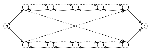
Figure 1: The graph $G_{r}$ with $r=5$. The solid arcs have cost 1 and the dashed arcs have cost 0.

Lemma 6.1.

The integrality gap of the LP ATSPP on the instance $F_{r}$ is at least $2-o(1)$.

Proof.

It is easy to verify that assigning $x_{a}=1/2$ to each arc that originally appeared in $G_{r}$ is a valid LP solution. Indeed, the degree constraints are immediate, and there are two edge-disjoint paths from $s$ to every other node in $G_{r}$ (so there must be at least 2 arcs exiting any subset containing $s$) so the cut constraints are also satisfied. The total cost of this LP solution is $r+1$.

On the other hand, we claim that the cost of any Hamiltonian $s$-$t$ path in $F_{r}$, which corresponds to a spanning $s$-$t$ walk $W$ in $G_{r}$, is at least $2r-1$. This shows an integrality gap of $\frac{2r-1}{r+1}=2-o(1)$.

To lower-bound the length of any spanning $s$-$t$ walk, we first argue that the walk $W$ can avoid using at most one of the unit cost arcs of the form $u_{i+1}u_{i}$ or $v_{i+1}v_{i}$. Indeed, any $u_{r}$-$v_{r}$ walk must use arcs $u_{i+1}u_{i}$ for every $1\leq i<r$. Similarly, every $v_{r}$-$u_{r}$ walk must use all arcs of the form $v_{i+1}v_{i}$. One of $u_{r}$ and $v_{r}$ is visited before the other, so either all of the $u_{i+1}u_{i}$ arcs or all of the $v_{i+1}v_{i}$ arcs are used by $W$. Now suppose, without loss of generality, that $W$ does not use the arcs $u_{i+1}u_{i}$ and $u_{j+1}u_{j}$ for $1\leq i<j<r$. Every $u_{i+1}$-$v_{r}$ walk uses arc $u_{i+1}u_{i}$ and every $v_{r}-u_{i+1}$ walk uses arc $u_{j+1}u_{j}$. Since one of $u_{i+1}$ or $v_{r}$ must be visited by $W$ before the other, then $W$ cannot avoid both $u_{i+1}u_{i}$ and $u_{j+1}u_{j}$ which contradicts our assumption.

Thus, $W$ must use all but at most one of the $2r-2$ unit cost arcs in $\{u_{i+1}u_{i}\mid 1\leq i<r\}\cup\{v_{i+1}v_{i}\mid 1\leq i<r\}$. Moreover, $W$ must also use one of the arcs exiting $s$ and one of the arcs entering $t$, so the cost of $W$ is at least $2r-1$. (In fact, the walk

$$\langle s,u_{1},v_{r},v_{r-1},\ldots,v_{1},u_{r},u_{r-1},\ldots,u_{3},u_{2},u_{3},\ldots,u_{r},t\rangle$$

is of length exactly $2r-1$, so this argument is tight.) ∎

7 Conclusion

In this paper we showed that the integrality gap for ATSPP is $O(\smash{\frac{\log n}{\log\log n}})$. We also show that a constant integrality gap bound follows from the form of Goddyn’s conjecture used in [18] to get an analogous ATSP integrality gap bound. We also showed a simpler construction achieving a lower bound of $2$ for the subtour elimination LP. One of the main open questions following this work is to show a more general reduction: does an $\alpha$ integrality gap bound for ATSP directly imply an $O(\alpha)$ integrality gap bound for ATSPP without any further assumptions?

Acknowledgments.

We thank V. Nagarajan for enlightening discussions in the early stages of this project. Z.F. and A.G. also thank A. Vetta and M. Singh for their generous hospitality. Part of this work was done when Z.F. was a postdoctoral fellow in the Department of Combinatorics and Optimization at the University of Waterloo, when A.G. was visiting the IEOR Department at Columbia University, and when M.S. was at McGill University. Finally, we thank anonymous reviewers for many helpful comments and the suggestion to obtain better bounds through thin tree conjectures.

References

- [1] H.-C. An, R. D. Kleinberg, and D. B. Shmoys. Improving Christofides’ algorithm for the - path TSP. In Proceedings of 44th ACM Symposium on Theory of Computing, 2012.
-
[2]
A. Asadpour, M. X. Goemans, A. M
dry, S. Oveis Gharan, and A. Saberi. An -approximation algorithm for the asymmetric traveling salesman problem. In Proceedings of the Twenty-First Annual ACM-SIAM Symposium on Discrete Algorithms, pages 379–389, 2010.‘ a - [3] M. Bateni and J. Chuzhoy. Approximation algorithms for the directed k-tour and k-stroll problems. In In Proceedings of 13th International Workshop on Approximation Algorithms for Combinatorial Optimization Problems, pages 25–38, 2010.
- [4] M. Bläser. A new approximation algorithm for the asymmetric TSP with triangle inequality. ACM Transactions of Algorithms, 4(4), 2008.
- [5] M. Charikar, M. X. Goemans, and H. Karloff. On the integrality ratio for the asymmetric traveling salesman problem. Mathematics of Operations Research, 31(2):245–252, 2006.
- [6] C. Chekuri and M. Pál. An approximation ratio for the asymmetric traveling salesman path problem. Theory of Computing, 3:197–209, 2007.
- [7] C. Chekuri, J. Vondrák, and R. Zenklusen. Dependent randomized rounding via exchange properties of combinatorial structures. In Proceedings of Annual IEEE Symposium on. Foundations of Computer Science, pages 575–584, 2010.
- [8] J. Edmonds. Submodular functions, matroids, and certain polyhedra. Combinatorial Structures and their Applications, pages 69–87, 1970.
- [9] U. Feige and M. Singh. Improved approximation ratios for traveling salesperson tours and paths in directed graphs. In 10th. International Workshop on Approximation Algorithms for Combinatorial Optimization Problems (APPROX), pages 104–118, 2007.
- [10] A. M. Frieze, G. Galbiati, and F. Maffioli. On the worst-case performance of some algorithms for the asymmetric traveling salesman problem. Networks, 12(1):23–39, 1982.
- [11] Z. Friggstad, M. R. Salavatipour, and Z. Svitkina. Asymmetric traveling salesman path and directed latency problems. In Proceedings of the Twenty-First Annual ACM-SIAM Symposium on Discrete Algorithms, pages 419–428, Philadelphia, PA, 2010. SIAM.
- [12] L. A. Goddyn. Some open problems i like. available at http://www.math.sfu.ca/ goddyn/ Problems/problems.html.
- [13] H. Kaplan, M. Lewenstein, N. Shafrir, and M. Sviridenko. Approximation algorithms for asymmetric TSP by decomposing directed regular multigraphs. Journal of the ACM, 52(4):602–626, 2005.
- [14] D. R. Karger and C. Stein. A new approach to the minimum cut problem. J. ACM, 43(4):601–640, 1996.
- [15] F. Lam and A. Newman. Traveling salesman path problems. Math. Program., 113(1, Ser. A):39–59, 2008.
- [16] V. Nagarajan and R. Ravi. Poly-logarithmic approximation algorithms for directed vehicle routing problems. In 10th. International Workshop on Approximation Algorithms for Combinatorial Optimization Problems (APPROX), pages 257–270, 2007.
- [17] V. Nagarajan and R. Ravi. The directed minimum latency problem. In Approximation, Randomization and Combinatorial Optimization, volume 5171 of Lecture Notes in Computer Science, pages 193–206. Springer, Berlin, 2008.
- [18] S. Oveis Gharan and A. Saberi. The asymmetric traveling salesman problem on graphs with bounded genus. In ACM-SIAM Symposium on Discrete Algorithms, pages 967–975, 2011.
- [19] A. Panconesi and A. Srinivasan. Randomized distributed edge coloring via an extension of the chernoff–hoeffding bounds. SIAM Journal on Computing, 26(2):350–368, 1997.
- [20] A. Schrijver. Combinatorial optimization. Polyhedra and efficiency., volume 24 of Algorithms and Combinatorics. Springer-Verlag, Berlin, 2003.
- [21] A. Sebő. Eight-fifth approximation for tsp paths. In Proceedings of The 16th Conference on Integer Programming and Combinatorial Optimization, 2013.
- [22] A. Sebő and J. Vygen. Shorter tours by nicer ears: -approximation for graphic TSP, for the path version, and for two-edge-connected subgraphs. CoRR, abs/1201.1870, 2012.