Information, Estimation, and Lookahead in the Gaussian channel

Kartik Venkat1, Tsachy Weissman1, Yair Carmon2, Shlomo Shamai2 1 Stanford University 2 Technion, Israel Institute of TechnologyPart of this work was presented at the 50th Annual Allerton Conference on Communications, Control and Computing, Monticello, Illinois, 2012.
Abstract

We consider mean squared estimation with lookahead of a continuous-time signal corrupted by additive white Gaussian noise. We show that the mutual information rate function, i.e., the mutual information rate as function of the signal-to-noise ratio (SNR), does not, in general, determine the minimum mean squared error (MMSE) with fixed finite lookahead, in contrast to the special cases with 0 and infinite lookahead (filtering and smoothing errors), respectively, which were previously established in the literature. We also establish a new expectation identity under a generalized observation model where the Gaussian channel has an SNR jump at t=0𝑑0t=0, capturing the tradeoff between lookahead and SNR.

Further, we study the class of continuous-time stationary Gauss-Markov processes (Ornstein-Uhlenbeck processes) as channel inputs, and explicitly characterize the behavior of the minimum mean squared error (MMSE) with finite lookahead and signal-to-noise ratio (SNR). The MMSE with lookahead is shown to converge exponentially rapidly to the non-causal error, with the exponent being the reciprocal of the non-causal error. We extend our results to mixtures of Ornstein-Uhlenbeck processes, and use the insight gained to present lower and upper bounds on the MMSE with lookahead for a class of stationary Gaussian input processes, whose spectrum can be expressed as a mixture of Ornstein-Uhlenbeck spectra.

Index Terms:
Mutual information, mean squared error (MSE), Brownian motion, Gaussian channel, additive white Gaussian noise (AWGN), causal/filtering error, non-causal/smoothing error, lookahead/delay, Ornstein-Uhlenbeck process, stationary process, power spectral density, signal-to-noise ratio (SNR)

I Introduction

Mean squared estimation of a signal in the presence of Gaussian noise has been a topic of considerable importance to the communities of information theory and estimation theory. There have further been discoveries tying the two fields together, through identities between fundamental informational quantities and the squared estimation loss.

Consider the continuous-time Gaussian channel. In [1], Duncan established the equivalence between the input-output mutual information and the integral of half the causal mean squared error in estimating the signal based on the observed process. In [2], Guo et al. present what is now known as the I-MMSE relationship, which equates the derivative of the mutual information rate to half the average non-causal squared error. These results were extended to incorporate mismatch at the decoder for the continuous-time Gaussian channel by Weissman in [3], building upon similar relations for the scalar Gaussian channel by VerdΓΊ in [4]. In [3], it was shown that when the decoder assumes an incorrect law for the input process, the difference in mismatched filtering loss is simply given by the relative entropy between the true and incorrect output distributions. Recently, in [5], a unified view of the aforementioned identities was presented. In particular, pointwise analogues of these and related results were developed, characterizing the original relationships as identities involving expectations of random objects with information-estimation significance of their own.

In this work, we shall focus on stationary continuous-time signals corrupted by Gaussian noise. Let 𝐗={Xt,tβˆˆβ„}𝐗subscript𝑋𝑑𝑑ℝ\mathbf{X}=\{X_{t},t\in\mathbb{R}\} denote a continuous-time signal, which is the channel input process. We assume square integrability of the stochastic process 𝐗𝐗\mathbf{X}, which says that for any finite interval [a,b]βŠ‚β„π‘Žπ‘β„[a,b]\subset\mathbb{R}, 𝔼​[∫abXt2​𝑑t]<βˆžπ”Όdelimited-[]superscriptsubscriptπ‘Žπ‘subscriptsuperscript𝑋2𝑑differential-d𝑑\mathbb{E}[\int_{a}^{b}X^{2}_{t}\,dt]<\infty.

The output process 𝐘𝐘\mathbf{Y} of the continuous-time Gaussian channel with input 𝐗𝐗\mathbf{X} is given by the following model

d​Yt=snr​Xt​d​t+d​Wt,𝑑subscriptπ‘Œπ‘‘snrsubscript𝑋𝑑𝑑𝑑𝑑subscriptπ‘Šπ‘‘dY_{t}=\sqrt{{\text{snr}}}\,X_{t}dt+dW_{t}, (1)

for all t𝑑t, where snr>0snr0{\text{snr}}>0 is the channel signal-to-noise ratio (SNR) and Wβ‹…subscriptπ‘Šβ‹…W_{\cdot} is a standard Brownian Motion (cf. [6] for definition and properties of Brownian motion) independent of 𝐗𝐗\mathbf{X}. For simplicity let us assume the input process to be stationary. Throughout, we will denote Xab={Xt:a≀t≀b}superscriptsubscriptπ‘‹π‘Žπ‘conditional-setsubscriptπ‘‹π‘‘π‘Žπ‘‘π‘X_{a}^{b}=\{X_{t}:a\leq t\leq b\}.

Let I​(snr)𝐼snrI({\text{snr}}) denote the mutual information rate, given by

I​(snr)=limTβ†’βˆž1T​I​(X0T;Y0T).𝐼snrsubscript→𝑇1𝑇𝐼superscriptsubscript𝑋0𝑇superscriptsubscriptπ‘Œ0𝑇\displaystyle I({\text{snr}})=\lim_{T\to\infty}\frac{1}{T}\,I(X_{0}^{T};Y_{0}^{T}). (2)

Let mmse​(snr)mmsesnr{\text{mmse}}({\text{snr}}) denote the smoothing squared error

mmse​(snr)=limTβ†’βˆž1Tβ€‹βˆ«0T𝔼​[(Xtβˆ’π”Όβ€‹[Xt|Y0T])2]​𝑑t,mmsesnrsubscript→𝑇1𝑇superscriptsubscript0𝑇𝔼delimited-[]superscriptsubscript𝑋𝑑𝔼delimited-[]conditionalsubscript𝑋𝑑superscriptsubscriptπ‘Œ0𝑇2differential-d𝑑\displaystyle{\text{mmse}}({\text{snr}})=\lim_{T\to\infty}\frac{1}{T}\int_{0}^{T}\mathbb{E}[(X_{t}-\mathbb{E}[X_{t}|Y_{0}^{T}])^{2}]\,dt, (3)

which, in our setting of stationarity, can equivalently be defined as

mmse​(snr)=𝔼​[(X0βˆ’π”Όβ€‹[X0|Yβˆ’βˆž+∞])2].mmsesnr𝔼delimited-[]superscriptsubscript𝑋0𝔼delimited-[]conditionalsubscript𝑋0superscriptsubscriptπ‘Œ2\displaystyle{\text{mmse}}({\text{snr}})=\mathbb{E}[(X_{0}-\mathbb{E}[X_{0}|Y_{-\infty}^{+\infty}])^{2}]. (4)

Similarly, the causal squared error is given by

cmmse​(snr)cmmsesnr\displaystyle{\text{cmmse}}({\text{snr}}) =\displaystyle= limTβ†’βˆž1Tβ€‹βˆ«0T𝔼​[(Xtβˆ’π”Όβ€‹[Xt|Y0t])2]​𝑑tsubscript→𝑇1𝑇superscriptsubscript0𝑇𝔼delimited-[]superscriptsubscript𝑋𝑑𝔼delimited-[]conditionalsubscript𝑋𝑑superscriptsubscriptπ‘Œ0𝑑2differential-d𝑑\displaystyle\lim_{T\to\infty}\frac{1}{T}\int_{0}^{T}\mathbb{E}[(X_{t}-\mathbb{E}[X_{t}|Y_{0}^{t}])^{2}]\,dt (5)
=\displaystyle= 𝔼​[(X0βˆ’π”Όβ€‹[X0|Yβˆ’βˆž0])2].𝔼delimited-[]superscriptsubscript𝑋0𝔼delimited-[]conditionalsubscript𝑋0superscriptsubscriptπ‘Œ02\displaystyle\mathbb{E}[(X_{0}-\mathbb{E}[X_{0}|Y_{-\infty}^{0}])^{2}]. (6)

From [1] and [2], we know that the above quantities are related according to

2​I​(snr)snr=cmmse​(snr)=1snrβ€‹βˆ«0snrmmse​(Ξ³)​𝑑γ2𝐼snrsnrcmmsesnr1snrsuperscriptsubscript0snrmmse𝛾differential-d𝛾\displaystyle\frac{2I({\text{snr}})}{{\text{snr}}}={\text{cmmse}}({\text{snr}})=\frac{1}{{\text{snr}}}\int_{0}^{{\text{snr}}}{\text{mmse}}(\gamma)\,d\gamma (7)

for all signal-to-noise ratios, snr>0snr0{\text{snr}}>0, and for all choices of the underlying input distribution111Indeed, (7) continues to hold in the absence of stationarity of the input process, in which case the respective quantities are averaged over a fixed, finite interval [0,T]0𝑇[0,T]. for which the process 𝐗𝐗\mathbf{X} is square integrable. Thus, the mutual information, the causal error and the non-causal error are linked together in a distribution independent fashion for the Gaussian channel under mean-squared loss. Having understood how the time averaged causal and non-causal errors behave, and in particular the relation (7) implying that they are completely characterized by the mutual information rate function - the current work seeks to address the question - what happens for lookahead between 00 and ∞\infty?.

The mean squared error with finite lookahead dβ‰₯0𝑑0d\geq 0 is defined as

lmmse​(d,snr)=𝔼​[(X0βˆ’π”Όβ€‹[X0|Yβˆ’βˆžd])2],lmmse𝑑snr𝔼delimited-[]superscriptsubscript𝑋0𝔼delimited-[]conditionalsubscript𝑋0superscriptsubscriptπ‘Œπ‘‘2\displaystyle{\text{lmmse}}(d,{\text{snr}})=\mathbb{E}[(X_{0}-\mathbb{E}[X_{0}|Y_{-\infty}^{d}])^{2}], (8)

where it is instructive to note that the special cases d=0𝑑0d=0 and d=βˆžπ‘‘d=\infty in (8) yield the filtering (6) and smoothing (4) errors respectively. Let us be slightly adventurous, and rewrite (7) as

2​I​(snr)snr=𝔼​[lmmse​(0,Ξ“0)]=𝔼​[lmmse​(∞,Ξ“βˆž)],2𝐼snrsnr𝔼delimited-[]lmmse0subscriptΞ“0𝔼delimited-[]lmmsesubscriptΞ“\displaystyle\frac{2I({\text{snr}})}{{\text{snr}}}=\mathbb{E}[{\text{lmmse}}(0,\Gamma_{0})]=\mathbb{E}[{\text{lmmse}}(\infty,\Gamma_{\infty})], (9)

where the random variables Ξ“0,Ξ“βˆžsubscriptΞ“0subscriptΞ“\Gamma_{0},\Gamma_{\infty} are distributed according to Ξ“0=snrsubscriptΞ“0snr\Gamma_{0}={\text{snr}} a.s., and Ξ“βˆžβˆΌU​[0,snr]similar-tosubscriptΞ“π‘ˆ0snr\Gamma_{\infty}\sim U[0,{\text{snr}}], where U​[a,b]π‘ˆπ‘Žπ‘U[a,b] denotes the uniform distribution on [a,b]π‘Žπ‘[a,b]. This characterization of the mutual information rate may lead one to conjecture the existence of a random variable Ξ“dsubscriptΓ𝑑\Gamma_{d}, whose distribution depends only on d,snr𝑑snrd,{\text{snr}}, and some features of the process (such as its bandwidth and spectrum), and satisfies the identity

2​I​(snr)snr=𝔼​[lmmse​(d,Ξ“d)],2𝐼snrsnr𝔼delimited-[]lmmse𝑑subscriptΓ𝑑\displaystyle\frac{2I({\text{snr}})}{{\text{snr}}}=\mathbb{E}[{\text{lmmse}}(d,\Gamma_{d})], (10)

regardless of the distribution of 𝐗𝐗\mathbf{X}. I.e., there exists a family of distributions Ξ“dsubscriptΓ𝑑\Gamma_{d} ranging from one extreme of a point mass at snr for d=0𝑑0d=0, to the uniform distribution over [0,snr]0snr[0,{\text{snr}}] when d=βˆžπ‘‘d=\infty. One of the corollaries of our results in this work is that such a relation cannot hold in general, even when allowing the distribution of Ξ“dsubscriptΓ𝑑\Gamma_{d} to depend on distribution-dependent features such as the process spectrum. In fact, in Section VII we show that in general, the mutual information rate function of a process is not sufficient to characterize the estimation error with finite lookahead. Therefore, one would need to consider features of the process that go beyond the mutual information rate and the spectrum - in order to characterize the finite lookahead estimation error. Motivated by this question, however, in Section VI we establish an identity which relates the filtering error to a double integral of the mean squared error, over lookahead and SNR, for the Gaussian channel with an SNR jump at t=0𝑑0t=0.

In the literature, finite lookahead estimation has been referred to as fixed-lag smoothing (cf., for example, [7] and references therein). Note that (8) is well defined for all dβˆˆβ„π‘‘β„d\in\mathbb{R}. For d<0𝑑0d<0, lmmse​(d,snr)lmmse𝑑snr{\text{lmmse}}(d,{\text{snr}}) denotes the finite horizon average prediction mean square error, which is as meaningful as its finite lookahead counterpart, i.e. the case when d>0𝑑0d>0. Motivated by the desire to understand the tradeoff between lookahead and mmse, in Section II we explicitly characterize this trade-off for the canonical family of continuous-time stationary Gauss-Markov (Ornstein-Uhlenbeck) processes. In particular, we find that the rate of convergence of lmmse​(β‹…,snr)lmmseβ‹…snr{\text{lmmse}}(\cdot,{\text{snr}}) with increasing lookahead (from causal to the non-causal error) is exponential, with the exponent given by the inverse of the non-causal error, i.e. 1mmse​(snr)1mmsesnr\frac{1}{{\text{mmse}}({\text{snr}})} itself.

The rest of the paper is organized as follows. In Section II we explicitly characterize the lookahead-MSE trade-off for the canonical family of continuous-time stationary Gauss-Markov (Ornstein-Uhlenbeck) processes. In particular, we find that the convergence of lmmse​(β‹…,snr)lmmseβ‹…snr{\text{lmmse}}(\cdot,{\text{snr}}) with increasing lookahead (from causal to the non-causal error) is exponentially fast, with the exponent given by the inverse of the non-causal error, i.e. 1mmse​(snr)1mmsesnr\frac{1}{{\text{mmse}}({\text{snr}})} itself. In Section III, we extend our results to a larger class of processes, that are expressible as a mixture of Ornstein-Uhlenbeck processes. We then consider stationary Gaussian input processes in Section IV, and characterize the MMSE with lookahead via spectral factorization methods. In Section V, we consider the information utility of infinitesimal lookahead for a general stationary input process and relate it to the squared filtering error. In Section VI, we introduce a generalized observation model for a stationary continuous-time signal where the channel has a non-stationary SNR jump at t=0𝑑0t=0. For this model, we establish an identity relating the squared error with finite lookahead and the causal filtering error. In Section VII, we show by means of an example that a distribution-independent identity of the form in (10) cannot hold in general. We conclude with a summary of our findings in Section VIII.

II Ornstein-Uhlenbeck Process

II-A Definitions and Properties

The Ornstein-Uhlenbeck process [8] is a classical continuous-time stochastic process characterized by the following stochastic differential equation

d​Xt=α​(ΞΌβˆ’Xt)​d​t+β​d​Bt,𝑑subscriptπ‘‹π‘‘π›Όπœ‡subscript𝑋𝑑𝑑𝑑𝛽𝑑subscript𝐡𝑑\displaystyle dX_{t}=\alpha(\mu-X_{t})dt+{\beta}dB_{t}, (11)

where {Bt}tβ‰₯0subscriptsubscript𝐡𝑑𝑑0\{B_{t}\}_{t\geq 0} is a Standard Brownian Motion and α𝛼\alpha, ΞΌπœ‡\mu, β𝛽\beta are process parameters. The reader is referred to [9] for a historical perspective on this process. Below, we present some of its important statistical properties. The mean and covariance functions are given by:

𝔼​(Xt)=ΞΌ,𝔼subscriptπ‘‹π‘‘πœ‡\mathbb{E}(X_{t})=\mu, (12)

and,

Cov​(Xt,Xs)Covsubscript𝑋𝑑subscript𝑋𝑠\displaystyle\text{Cov}(X_{t},X_{s}) =Ξ²22​α​eβˆ’Ξ±β€‹|tβˆ’s|.absentsuperscript𝛽22𝛼superscript𝑒𝛼𝑑𝑠\displaystyle=\frac{\beta^{2}}{2\alpha}e^{-\alpha|t-s|}. (13)

We can further denote the autocorrelation function and power spectral density of this process by

RX​(Ο„)subscriptπ‘…π‘‹πœ\displaystyle R_{X}(\tau) =Ξ²22​α​eβˆ’Ξ±β€‹|Ο„|,absentsuperscript𝛽22𝛼superscriptπ‘’π›Όπœ\displaystyle=\frac{\beta^{2}}{2\alpha}e^{-\alpha|\tau|}, (14)
SX​(Ο‰)subscriptπ‘†π‘‹πœ”\displaystyle S_{X}(\omega) =Ξ²2Ξ±2+Ο‰2.absentsuperscript𝛽2superscript𝛼2superscriptπœ”2\displaystyle=\frac{\beta^{2}}{\alpha^{2}+\omega^{2}}. (15)

In all further analysis, we consider the process mean ΞΌπœ‡\mu to be 0. We also note that all expressions are provided assuming Ξ±>0𝛼0\alpha>0 which results in a mean-reverting evolution of the process.

II-B Mean Squared Estimation Error

Recall the mean squared error with finite lookahead d𝑑d defined in (8) from which one can infer the filtering (6) and smoothing (4) errors respectively. We now compute these quantities for the Ornstein-Uhlenbeck process at a fixed signal to noise ratio γ𝛾\gamma. Define, for the Ornstein-Uhlenbeck process corrupted by the Gaussian channel (1), the error in estimating X0subscript𝑋0X_{0} based on a finite lookahead d𝑑d into the future and a certain lookback l𝑙l into the past:

ν​(l,d,Ξ³)=Var​(X0|Yβˆ’ld)d,lβ‰₯0.formulae-sequenceπœˆπ‘™π‘‘π›ΎVarconditionalsubscript𝑋0superscriptsubscriptπ‘Œπ‘™π‘‘π‘‘π‘™0\displaystyle\nu(l,d,\gamma)={\text{Var}}(X_{0}|Y_{-l}^{d})\hskip 10.00002ptd,l\geq 0. (16)

Before we explicitly characterize ν​(l,d,Ξ³)πœˆπ‘™π‘‘π›Ύ\nu(l,d,\gamma), we present the following intermediate result, which is proved in Appendix A.

Lemma 1

Let ed=ν​(0,d,Ξ³)=ν​(d,0,Ξ³)subscriptπ‘’π‘‘πœˆ0π‘‘π›Ύπœˆπ‘‘0𝛾e_{d}=\nu(0,d,\gamma)=\nu(d,0,\gamma)222where the latter equality holds due to time-reversibility of the Ornstein-Uhlenbeck process. Then,

ed=Ξ›d​α2+γ​β2βˆ’Ξ±Ξ³,subscript𝑒𝑑subscriptΛ𝑑superscript𝛼2𝛾superscript𝛽2𝛼𝛾e_{d}=\frac{\Lambda_{d}\sqrt{\alpha^{2}+\gamma{\beta^{2}}}-\alpha}{\gamma}, (17)

where Ξ›d=e2​d​α2+γ​β2​ρ+1e2​d​α2+γ​β2β€‹Οβˆ’1subscriptΛ𝑑superscript𝑒2𝑑superscript𝛼2𝛾superscript𝛽2𝜌1superscript𝑒2𝑑superscript𝛼2𝛾superscript𝛽2𝜌1\Lambda_{d}=\frac{e^{2d\sqrt{\alpha^{2}+\gamma{\beta^{2}}}}\rho+1}{e^{2d\sqrt{\alpha^{2}+\gamma{\beta^{2}}}}\rho-1} and ρ=|γ​RX​(0)+Ξ±2+γ​β2+αγ​RX​(0)βˆ’Ξ±2+γ​β2+Ξ±|πœŒπ›Ύsubscript𝑅𝑋0superscript𝛼2𝛾superscript𝛽2𝛼𝛾subscript𝑅𝑋0superscript𝛼2𝛾superscript𝛽2𝛼\rho=\left|\frac{\gamma R_{X}(0)+{\sqrt{\alpha^{2}+\gamma{\beta^{2}}}+\alpha}}{\gamma R_{X}(0)-\sqrt{\alpha^{2}+\gamma{\beta^{2}}}+\alpha}\right|.

Using Lemma 1, we now compute the more general quantity ν​(l,d,Ξ³)πœˆπ‘™π‘‘π›Ύ\nu(l,d,\gamma) defined in (16), which denotes the loss in estimating Xtsubscript𝑋𝑑X_{t} based on the observations Ytβˆ’dt+lsuperscriptsubscriptπ‘Œπ‘‘π‘‘π‘‘π‘™Y_{t-d}^{t+l}, for a stationary process.

Lemma 2 (estimation error with finite window of observations in the past and future)
ν​(l,d,Ξ³)=el​ed​RX​(0)RX​(0)​(el+ed)βˆ’el​ed.πœˆπ‘™π‘‘π›Ύsubscript𝑒𝑙subscript𝑒𝑑subscript𝑅𝑋0subscript𝑅𝑋0subscript𝑒𝑙subscript𝑒𝑑subscript𝑒𝑙subscript𝑒𝑑\displaystyle\nu(l,d,\gamma)=\frac{e_{l}e_{d}R_{X}(0)}{R_{X}(0)(e_{l}+e_{d})-e_{l}e_{d}}. (18)

The proof of Lemma 2 is straightforward, upon noting (i) the Markov Chain relationship Yβˆ’l0βˆ’X0βˆ’Y0dsuperscriptsubscriptπ‘Œπ‘™0subscript𝑋0superscriptsubscriptπ‘Œ0𝑑Y_{-l}^{0}\--X_{0}\--{Y_{0}^{d}}, and (ii) the joint Gaussianity of (X0,Yβˆ’ldsubscript𝑋0superscriptsubscriptπ‘Œπ‘™π‘‘X_{0},Y_{-l}^{d}). Thus, one can use the conditional variances Var​(X0|Yβˆ’l0)Varconditionalsubscript𝑋0superscriptsubscriptπ‘Œπ‘™0{\text{Var}}(X_{0}|Y_{-l}^{0}) and Var​(X0|Y0d)Varconditionalsubscript𝑋0superscriptsubscriptπ‘Œ0𝑑{\text{Var}}(X_{0}|Y_{0}^{d}) to obtain the required expression for Var​(X0|Yβˆ’ld)Varconditionalsubscript𝑋0superscriptsubscriptπ‘Œπ‘™π‘‘{\text{Var}}(X_{0}|Y_{-l}^{d}).

Using Lemma 1 and Lemma 2 we explicitly characterize the filtering (6) and smoothing (4) (mean squared error) MSE’s for the noise corrupted Ornstein-Uhlenbeck process, in the following Lemma.

Lemma 3 (MSE for the Ornstein-Ulhenbeck process)

For the Ornstein-Ulhenbeck process corrupted by white gaussian noise at signal-to-noise ratio snr, the filtering and smoothing errors are given by:

  • β€’

    Filtering Error

    cmmse​(snr)=ν​(∞,0,snr)=Ξ±2+snr​β2βˆ’Ξ±snrcmmsesnr𝜈0snrsuperscript𝛼2snrsuperscript𝛽2𝛼snr\displaystyle{\text{cmmse}}({\text{snr}})=\nu(\infty,0,{\text{snr}})=\frac{\sqrt{\alpha^{2}+{\text{snr}}{\beta^{2}}}-\alpha}{{\text{snr}}} (19)
  • β€’

    Smoothing Error

    mmse​(snr)=ν​(∞,∞,snr)=Ξ²22​α2+snr​β2.mmsesnr𝜈snrsuperscript𝛽22superscript𝛼2snrsuperscript𝛽2\displaystyle{\text{mmse}}({\text{snr}})=\nu(\infty,\infty,{\text{snr}})=\frac{\beta^{2}}{2\sqrt{\alpha^{2}+{\text{snr}}{\beta^{2}}}}. (20)

The expressions in (19) and (20) recover the classical expressions for the optimal causal and smoothing errors (for Gaussian inputs), due to Yovits and Jackson in [12], and Wiener in [13], respectively.

Remark: (19) and (20) can be easily seen to verify the following general relationship between the filtering and smoothing error for the continuous time Gaussian channel, established in [2], i.e.

cmmse​(snr)cmmsesnr\displaystyle{\text{cmmse}}({\text{snr}}) =\displaystyle= 1snrβ€‹βˆ«0snrmmse​(Ξ³)​𝑑γ.1snrsuperscriptsubscript0snrmmse𝛾differential-d𝛾\displaystyle\frac{1}{{\text{snr}}}\int_{0}^{{\text{snr}}}{\text{mmse}}(\gamma)\,d\gamma. (21)

II-C Estimation with Lookahead

Having introduced the Ornstein-Ulhenbeck process and its properties, we now study the behavior of the MMSE with finite lookahead.
Note: For the rest of this paper we will set Ξ²=1𝛽1\beta=1 in (11), as it only involves an effective scaling of the channel SNR parameter.

Recall that,

lmmse​(d,Ξ³)lmmse𝑑𝛾\displaystyle{\text{lmmse}}(d,\gamma) =Var​(X0|Yβˆ’βˆžd)absentVarconditionalsubscript𝑋0superscriptsubscriptπ‘Œπ‘‘\displaystyle={\text{Var}}(X_{0}|Y_{-\infty}^{d}) (22)
=ν​(∞,d,Ξ³),absentπœˆπ‘‘π›Ύ\displaystyle=\nu(\infty,d,\gamma), (23)

where (23) follows from the definition of ν​(β‹…,β‹…,Ξ³)πœˆβ‹…β‹…π›Ύ\nu(\cdot,\cdot,\gamma) in Lemma 2. The following lemma explicitly characterizes the finite lookahead MMSE for the Ornstein-Ulhenbeck process with parameter α𝛼\alpha, corrupted by the Gaussian channel at signal-to-noise ratio γ𝛾\gamma.

Lemma 4 (MMSE with Lookahead for OU(α𝛼\alpha))
lmmse​(d,Ξ³)={(1βˆ’eβˆ’2​d​α2+Ξ³)​mmse​(Ξ³)+eβˆ’2​d​α2+γ​cmmse​(Ξ³)if ​dβ‰₯0eβˆ’2​α​|d|​cmmse​(Ξ³)+12​α​(1βˆ’eβˆ’2​α​|d|)if ​d<0.lmmse𝑑𝛾cases1superscript𝑒2𝑑superscript𝛼2𝛾mmse𝛾superscript𝑒2𝑑superscript𝛼2𝛾cmmse𝛾if 𝑑0superscript𝑒2𝛼𝑑cmmse𝛾12𝛼1superscript𝑒2𝛼𝑑if 𝑑0\displaystyle{\text{lmmse}}(d,\gamma)=\left\{\begin{array}[]{ll}(1-e^{-2d\sqrt{\alpha^{2}+\gamma}})\text{mmse}(\gamma)+e^{-2d\sqrt{\alpha^{2}+\gamma}}\text{cmmse}(\gamma)&\mbox{if }d\geq 0\\ e^{-2\alpha|d|}\text{cmmse}(\gamma)+\frac{1}{2\alpha}(1-e^{-2\alpha|d|})&\mbox{if }d<0.\end{array}\right. (26)
Proof:

We will establish the expression for positive and negative values lookahead separately.

For dβ‰₯0𝑑0d\geq 0: We combine (22) and Lemma 2 to obtain the closed form expression for lmmse​(d,Ξ³)lmmse𝑑𝛾{\text{lmmse}}(d,\gamma). In addition, from Lemma 3 we note that

cmmse​(Ξ³)cmmse𝛾\displaystyle\text{cmmse}(\gamma) =\displaystyle= Ξ±2+Ξ³βˆ’Ξ±Ξ³,superscript𝛼2𝛾𝛼𝛾\displaystyle\frac{\sqrt{\alpha^{2}+\gamma}-\alpha}{\gamma}, (27)
mmse​(Ξ³)mmse𝛾\displaystyle\text{mmse}(\gamma) =\displaystyle= 12​α2+Ξ³.12superscript𝛼2𝛾\displaystyle\frac{1}{2\sqrt{\alpha^{2}+\gamma}}. (28)

Using the above expressions, we can express the estimation error with finite lookahead dβ‰₯0𝑑0d\geq 0 in the following succinct manner

lmmse​(d,Ξ³)lmmse𝑑𝛾\displaystyle{\text{lmmse}}(d,\gamma) =\displaystyle= (1βˆ’eβˆ’2​d​α2+Ξ³)​mmse​(Ξ³)+eβˆ’2​d​α2+γ​cmmse​(Ξ³).1superscript𝑒2𝑑superscript𝛼2𝛾mmse𝛾superscript𝑒2𝑑superscript𝛼2𝛾cmmse𝛾\displaystyle(1-e^{-2d\sqrt{\alpha^{2}+\gamma}})\text{mmse}(\gamma)+e^{-2d\sqrt{\alpha^{2}+\gamma}}\text{cmmse}(\gamma). (29)

For d<0𝑑0d<0: We denote the absolute value of d𝑑d as |d|𝑑|d|, and note that

Yβˆ’βˆžβˆ’|d|βˆ’Xβˆ’|d|βˆ’X0superscriptsubscriptπ‘Œπ‘‘subscript𝑋𝑑subscript𝑋0\displaystyle Y_{-\infty}^{-|d|}\--X_{-|d|}\--{X_{0}} (30)

forms a Markov triplet. We further note that (X0,Xβˆ’|d|,Yβˆ’βˆžβˆ’|d|subscript𝑋0subscript𝑋𝑑superscriptsubscriptπ‘Œπ‘‘X_{0},X_{-|d|},Y_{-\infty}^{-|d|}) are jointly Gaussian. In particular, we know that

X0|Xβˆ’|d|conditionalsubscript𝑋0subscript𝑋𝑑\displaystyle X_{0}|X_{-|d|} βˆΌπ’©β€‹(Xβˆ’|d|​eβˆ’Ξ±β€‹|d|,12​α​(1βˆ’eβˆ’2​α​|d|)),similar-toabsent𝒩subscript𝑋𝑑superscript𝑒𝛼𝑑12𝛼1superscript𝑒2𝛼𝑑\displaystyle\sim{\cal N}\bigg{(}X_{-|d|}e^{-\alpha|d|},\frac{1}{2\alpha}(1-e^{-2\alpha|d|})\bigg{)}, (31)
Var​(Xβˆ’|d||Yβˆ’βˆžβˆ’|d|)Varconditionalsubscript𝑋𝑑superscriptsubscriptπ‘Œπ‘‘\displaystyle{\text{Var}}(X_{-|d|}|Y_{-\infty}^{-|d|}) =cmmse​(Ξ³)absentcmmse𝛾\displaystyle=\text{cmmse}(\gamma) (32)

From the above relations, it is easy to arrive at the required quantity Var​(X0|Yβˆ’βˆžβˆ’|d|)Varconditionalsubscript𝑋0superscriptsubscriptπ‘Œπ‘‘{\text{Var}}(X_{0}|Y_{-\infty}^{-|d|}) for d<0𝑑0d<0,

lmmse​(d,Ξ³)lmmse𝑑𝛾\displaystyle{\text{lmmse}}(d,\gamma) =\displaystyle= eβˆ’2​α​|d|​cmmse​(Ξ³)+12​α​(1βˆ’eβˆ’2​α​|d|).superscript𝑒2𝛼𝑑cmmse𝛾12𝛼1superscript𝑒2𝛼𝑑\displaystyle e^{-2\alpha|d|}\text{cmmse}(\gamma)+\frac{1}{2\alpha}(1-e^{-2\alpha|d|}). (33)

This completes the proof. ∎

Refer to caption
Figure 1: lmmse​(d,snr)lmmse𝑑snr{\text{lmmse}}(d,{\text{snr}}) vs. lookahead d𝑑d for the Ornstein-Uhlenbeck process for Ξ±=0.5𝛼0.5\alpha=0.5, and snr=1snr1{\text{snr}}=1.

A plot of the estimation error with finite lookahead for the Ornstein-Uhlenbeck process is shown in Fig. 1. It is seen from the expression in Lemma 4, that the asymptotes at d=βˆ’βˆžπ‘‘d=-\infty and d=+βˆžπ‘‘d=+\infty correspond to the values RX​(0)subscript𝑅𝑋0R_{X}(0) and mmse​(snr)mmsesnr{\text{mmse}}({\text{snr}}), respectively, for a fixed SNR level snr.

We now focus on the case where dβ‰₯0𝑑0d\geq 0, which corresponds to estimation with finite delay. We define, for dβ‰₯0𝑑0d\geq 0,

pd≐lmmse​(d,Ξ³)βˆ’mmse​(Ξ³)cmmse​(Ξ³)βˆ’mmse​(Ξ³).approaches-limitsubscript𝑝𝑑lmmse𝑑𝛾mmse𝛾cmmse𝛾mmse𝛾\displaystyle p_{d}\doteq\frac{{\text{lmmse}}(d,\gamma)-{\text{mmse}}(\gamma)}{{\text{cmmse}}(\gamma)-{\text{mmse}}(\gamma)}. (34)

From Lemma 4, we observe that for the Ornstein-Ulhenbeck process,

pdsubscript𝑝𝑑\displaystyle p_{d} =\displaystyle= eβˆ’2​d​α2+Ξ³superscript𝑒2𝑑superscript𝛼2𝛾\displaystyle e^{-2d\sqrt{\alpha^{2}+\gamma}} (35)
=\displaystyle= eβˆ’dmmse​(Ξ³),superscript𝑒𝑑mmse𝛾\displaystyle e^{-\frac{d}{\text{mmse}{(\gamma)}}}, (36)

where (36) follows from (28). In other words, the causal error approaches the non-causal error exponentially fast with increasing lookahead. This conveys the importance of lookahead in signal estimation with finite delay. We can state this observation as follows:

Observation 5

For any AWGN corrupted Ornstein-Ulhenbeck process, the mean squared error with finite positive lookahead, approaches the non-causal error exponentially fast, with decay exponent given by 1mmse​(Ξ³)1mmse𝛾\frac{1}{\text{mmse}(\gamma)}.

II-D SNR vs Lookahead tradeoff

One way to quantify the utility of lookahead in finite delay estimation is to compute the corresponding gain in SNR. Specifically, we compute the required SNR level which gives the same mmse with lookahead d𝑑d as the filtering error at a fixed SNR level snr>0snr0{\text{snr}}>0.

Let Ξ³dβˆ—β€‹(snr)subscriptsuperscript𝛾𝑑snr\gamma^{*}_{d}({\text{snr}}) be the value of β€˜signal to noise ratio’ that provides the same mean square error as the causal filter with zero lookahead. I.e.

lmmse​(d,Ξ³dβˆ—β€‹(snr))=cmmse​(snr),lmmse𝑑subscriptsuperscript𝛾𝑑snrcmmsesnr\displaystyle{\text{lmmse}}(d,\gamma^{*}_{d}({\text{snr}}))={\text{cmmse}}({\text{snr}}), (37)

whenever a solution Ξ³dβˆ—β€‹(snr)>0subscriptsuperscript𝛾𝑑snr0\gamma^{*}_{d}({\text{snr}})>0 exists.

We now present some general observations about Ξ³dβˆ—β€‹(snr)subscriptsuperscript𝛾𝑑snr\gamma^{*}_{d}({\text{snr}}).

  • β€’

    Ξ³dβˆ—β€‹(snr)subscriptsuperscript𝛾𝑑snr\gamma^{*}_{d}({\text{snr}}) is a monotonically decreasing function of d𝑑d.

  • β€’

    Ξ³0βˆ—β€‹(snr)=snrsubscriptsuperscript𝛾0snrsnr\gamma^{*}_{0}({\text{snr}})={\text{snr}}.

  • β€’

    Let Ξ³βˆžβ€‹(snr)=limdβ†’βˆžΞ³dβˆ—β€‹(snr)subscript𝛾snrsubscript→𝑑subscriptsuperscript𝛾𝑑snr\gamma_{\infty}({\text{snr}})=\lim_{d\to\infty}\gamma^{*}_{d}({\text{snr}}). Then, we have mmse​(Ξ³βˆžβ€‹(snr))=cmmse​(snr)mmsesubscript𝛾snrcmmsesnr{\text{mmse}}(\gamma_{\infty}({\text{snr}}))={\text{cmmse}}({\text{snr}}). For the Ornstein-Uhlenbeck process parameterized by α𝛼\alpha, we get the following closed form expression for Ξ³βˆžβ€‹(snr)subscript𝛾snr\gamma_{\infty}({\text{snr}}):

    Ξ³βˆžβ€‹(snr)subscript𝛾snr\displaystyle\gamma_{\infty}({\text{snr}}) =\displaystyle= 1(2​cmmse​(snr))2βˆ’Ξ±2.1superscript2cmmsesnr2superscript𝛼2\displaystyle\frac{1}{(2{\text{cmmse}}({\text{snr}}))^{2}}-\alpha^{2}. (38)
  • β€’

    Ξ³dβˆ—β€‹(snr)subscriptsuperscript𝛾𝑑snr\gamma^{*}_{d}({\text{snr}}) has a vertical asymptote at d=dsnrβˆ—<0𝑑subscriptsuperscript𝑑snr0d=d^{*}_{{\text{snr}}}<0, where dsnrβˆ—subscriptsuperscript𝑑snrd^{*}_{{\text{snr}}} is defined as the solution to the equation Var(X0|Xdsnrβˆ—conditionalsubscript𝑋0subscript𝑋subscriptsuperscript𝑑snrX_{0}|X_{d^{*}_{{\text{snr}}}}) = cmmse​(snr)cmmsesnr{\text{cmmse}}({\text{snr}}). Then we have,

    limdβ†’ds​n​rβˆ—Ξ³dβˆ—β€‹(snr)=∞subscript→𝑑subscriptsuperscriptπ‘‘π‘ π‘›π‘Ÿsubscriptsuperscript𝛾𝑑snr\displaystyle\lim_{d\to d^{*}_{snr}}\gamma^{*}_{d}({\text{snr}})=\infty (39)

In Fig. 2, we illustrate the behavior of Ξ³d​(snr)subscript𝛾𝑑snr\gamma_{d}({\text{snr}}) as a function of lookahead, for the Ornstein-Uhlenbeck process corrupted by Gaussian noise according to the channel in (1).

Refer to caption
Figure 2: Plot of Ξ³dβˆ—β€‹(snr)subscriptsuperscript𝛾𝑑snr\gamma^{*}_{d}({\text{snr}}) (snr=1snr1{\text{snr}}=1) as a function of d𝑑d for the Ornstein Uhlenbeck process with parameter Ξ±=0.2𝛼0.2\alpha=0.2. In this case γ∞subscript𝛾\gamma_{\infty} = 0.3320 and dβˆ—=βˆ’0.9935superscript𝑑0.9935d^{*}=-0.9935.

III A mixture of Ornstein-Uhlenbeck processes

Having presented the finite lookahead MMSE for the Ornstein-Ulhenbeck process in Lemma 4, in this section we obtain the MMSE with lookahead for the class of stochastic processes that are mixtures of Ornstein-Ulhenbeck processes. We then proceed to establish a general lower bound on the MMSE with lookahead for the class Gaussian processes whose spectra can be decomposed as a mixture of spectra of Ornstein-Ulhenbeck processes. For the same class of Gaussian processes, we also present an upper bound for the finite lookahead MMSE, in terms of a mismatched estimation loss.

Let μ​(Ξ±)πœ‡π›Ό\mu(\alpha) be a probability measure defined on [0,∞)0[0,\infty). Let P(Ξ±)superscript𝑃𝛼P^{(\alpha)} be the law of the Ornstein-Uhlenbeck process with parameter α𝛼\alpha. Note that each P(Ξ±)superscript𝑃𝛼P^{(\alpha)} is the law of a stationary ergodic stochastic process. We define the stationary distribution generated by taking a ΞΌπœ‡\mu-mixture of these processes:

P=∫P(Ξ±)​𝑑μ​(Ξ±).𝑃superscript𝑃𝛼differential-dπœ‡π›Ό\displaystyle P=\int P^{(\alpha)}\,d\mu(\alpha). (40)

Note that P𝑃P need not be Gaussian in general.

Lemma 6

Let X𝑋X be a stationary stochastic process governed by law P𝑃P which is a ΞΌπœ‡\mu mixture of Ornstein-Ulhenbeck processes, and is corrupted by AWGN at SNR γ𝛾\gamma. The MMSE with finite lookahead d𝑑d is given by

lmmseP​(d,Ξ³)=∫lmmseα​(d,Ξ³)​𝑑μ​(Ξ±),subscriptlmmse𝑃𝑑𝛾subscriptlmmse𝛼𝑑𝛾differential-dπœ‡π›Ό\displaystyle{\text{lmmse}}_{P}(d,\gamma)=\int{\text{lmmse}}_{\alpha}(d,\gamma)\,d\mu({\alpha}), (41)

where lmmseα​(d,Ξ³)subscriptlmmse𝛼𝑑𝛾{\text{lmmse}}_{\alpha}(d,\gamma) is (as defined in Lemma 4) the corresponding quantity for estimating an Ornstein-Ulhenbeck process with parameter α𝛼\alpha.

The proof of Lemma 6 follows in one line, upon observing that the underlying β€˜active mode’ is eventually precisely learned from the infinitely long observation of the noisy process. This relation allows us to compute the minimum mean squared error with finite lookahead for the large class of processes that can be expressed as mixtures of Ornstein-Uhlenbeck processes.

As another important corollary of this discussion, consider any Gaussian process G𝐺G whose spectrum SGsubscript𝑆𝐺S_{G} can be expressed as a mixture of spectra of Ornstein-Uhlenbeck processes, for some appropriate mixing measure μ​(Ξ±)πœ‡π›Ό\mu(\alpha),i.e.

SG=∫Sα​𝑑μ​(Ξ±),subscript𝑆𝐺subscript𝑆𝛼differential-dπœ‡π›Ό\displaystyle S_{G}=\int S_{\alpha}\,d\mu(\alpha), (42)

where SΞ±subscript𝑆𝛼S_{\alpha} denotes the spectrum of the Ornstein-Ulhenbeck process with parameter α𝛼\alpha. The approach outlined above provides us with a computable lower bound on the minimum mean squared error with fixed lookahead d𝑑d (under AWGN) for the process G𝐺G, which we state in the following Lemma.

Lemma 7

For a Gaussian process G𝐺G with spectrum as in (42), the finite lookahead mmse has the following lower bound:

lmmseG​(d,Ξ³)β‰₯∫lmmseα​(d,Ξ³)​𝑑μ​(Ξ±),subscriptlmmse𝐺𝑑𝛾subscriptlmmse𝛼𝑑𝛾differential-dπœ‡π›Ό\displaystyle{\text{lmmse}}_{G}(d,\gamma)\geq\int{\text{lmmse}}_{\alpha}(d,\gamma)\,d\mu(\alpha), (43)

where lmmseα​(d,Ξ³)subscriptlmmse𝛼𝑑𝛾{\text{lmmse}}_{\alpha}(d,\gamma) is characterized explicitly in Lemma 4.

To see why (43) holds note that its right hand side represents the mmse at lookahead d𝑑d associated with the process whose law is expressed in (40), while the left side corresponds to this mmse under a Gaussian source with the same spectrum.

In the following example, we will illustrate the bound in (43). In Section IV-A, we discuss the computation of the mmse with lookahead for any stationary Gaussian process, of a known spectrum. This computation, based on Wiener-Kolmogorov theory, relies on the spectral factorization of the spectrum of the AWGN corrupted process. This factorization is, in general, difficult to perform. Thus, a bound on the mmse with lookahead, such as in (43), for a Gaussian process whose spectrum can be expressed as a mixture of spectra of Ornstein-Ulhenbeck processes, is quite useful.

A natural question that emerges from the above discussion is, what functions can be decomposed into mixtures of spectra of Ornstein-Ulhenbeck processes ? To answer this question, note that one can arrive at any spectrum SGsubscript𝑆𝐺S_{G} which can be expressed (upto a multiplicative constant) as

SG​(Ο‰)=∫0∞1Ξ±2+Ο‰2​𝑑μ​(Ξ±)subscriptπ‘†πΊπœ”superscriptsubscript01superscript𝛼2superscriptπœ”2differential-dπœ‡π›Ό\displaystyle S_{G}(\omega)=\int_{0}^{\infty}\frac{1}{\alpha^{2}+\omega^{2}}\,d\mu(\alpha) (44)

where we use (15) to characterize Sα​(Ο‰)subscriptπ‘†π›Όπœ”S_{\alpha}(\omega). Equivalently, in the time domain, the desired auto-correlation function is expressible as

RG​(Ο„)=∫0∞eβˆ’Ξ±β€‹|Ο„|​d​μ​(Ξ±)Ξ±,subscriptπ‘…πΊπœsuperscriptsubscript0superscriptπ‘’π›Όπœπ‘‘πœ‡π›Όπ›Ό\displaystyle R_{G}(\tau)=\int_{0}^{\infty}e^{-\alpha|\tau|}\,\frac{d\mu(\alpha)}{\alpha}, (45)

which can be viewed as a real-exponential transform of the function ΞΌπœ‡\mu. However, as can be seen from (44), the spectrum SG​(Ο‰)subscriptπ‘†πΊπœ”S_{G}(\omega) is always constrained to be monotonically decreasing with Ο‰πœ”\omega. This shows that the space of functions that can be candidates for the spectrum of the process G, is not exhausted by the class of functions decomposable as spectra of Ornstein-Ulhenbeck processes.

III-A Illustration of bound in Lemma 7

We consider the simple scenario of a process which is the equal mixture of two Ornstein-Ulhenbeck processes, 𝐗1subscript𝐗1\mathbf{X}_{1} and 𝐗2subscript𝐗2\mathbf{X}_{2}, parametrized by Ξ±1subscript𝛼1\alpha_{1} and Ξ±2subscript𝛼2\alpha_{2} respectively. Specifically, let us define a stationary continous-time process 𝐗𝐗\mathbf{X} as

𝐗={𝐗1ifΒ w.p.​12𝐗2ifΒ w.p.​12𝐗casessubscript𝐗1ifΒ w.p.12subscript𝐗2ifΒ w.p.12\displaystyle\mathbf{X}=\left\{\begin{array}[]{ll}\mathbf{X}_{1}&\mbox{if }\text{w.p.}\frac{1}{2}\\ \mathbf{X}_{2}&\mbox{if }\text{w.p.}\frac{1}{2}\end{array}\right. (48)

Note that the process 𝐗𝐗\mathbf{X} will not be Gaussian in general. The spectrum S𝐗​(β‹…)subscript𝑆𝐗⋅S_{\mathbf{X}}(\cdot) of the mixture, will be given by the mixture of the spectra of the constituent Ornstein-Ulhenbeck processes. I.e.

S𝐗​(β‹…)=12​S𝐗1​(β‹…)+12​S𝐗2​(β‹…),subscript𝑆𝐗⋅12subscript𝑆subscript𝐗1β‹…12subscript𝑆subscript𝐗2β‹…\displaystyle S_{\mathbf{X}}(\cdot)=\frac{1}{2}S_{\mathbf{X}_{1}}(\cdot)+\frac{1}{2}S_{\mathbf{X}_{2}}(\cdot), (49)

where S𝐗isubscript𝑆subscript𝐗𝑖S_{\mathbf{X}_{i}}, denotes the spectrum of 𝐗isubscript𝐗𝑖\mathbf{X}_{i}, i=1,2𝑖12i=1,2. Now consider a stationary Gaussian process 𝐆𝐆\mathbf{G} with the same spectrum, i.e.

S𝐆​(β‹…)=S𝐗​(β‹…).subscript𝑆𝐆⋅subscript𝑆𝐗⋅\displaystyle S_{\mathbf{G}}(\cdot)=S_{\mathbf{X}}(\cdot). (50)

We will consider the noise corruption mechanism in (1) at a signal-to-noise ratio snr. Note that Lemma 4, in conjunction with (41), allow us to compute the mmse with lookahead lmmse𝐗​(d,snr)subscriptlmmse𝐗𝑑snr{\text{lmmse}}_{\mathbf{X}}(d,{\text{snr}}), for the 𝐗𝐗\mathbf{X} process:

lmmse𝐗​(d,snr)=12​lmmse𝐗1​(d,snr)+12​lmmse𝐗2​(d,snr),subscriptlmmse𝐗𝑑snr12subscriptlmmsesubscript𝐗1𝑑snr12subscriptlmmsesubscript𝐗2𝑑snr\displaystyle{\text{lmmse}}_{\mathbf{X}}(d,{\text{snr}})=\frac{1}{2}{\text{lmmse}}_{\mathbf{X}_{1}}(d,{\text{snr}})+\frac{1}{2}{\text{lmmse}}_{\mathbf{X}_{2}}(d,{\text{snr}}), (51)

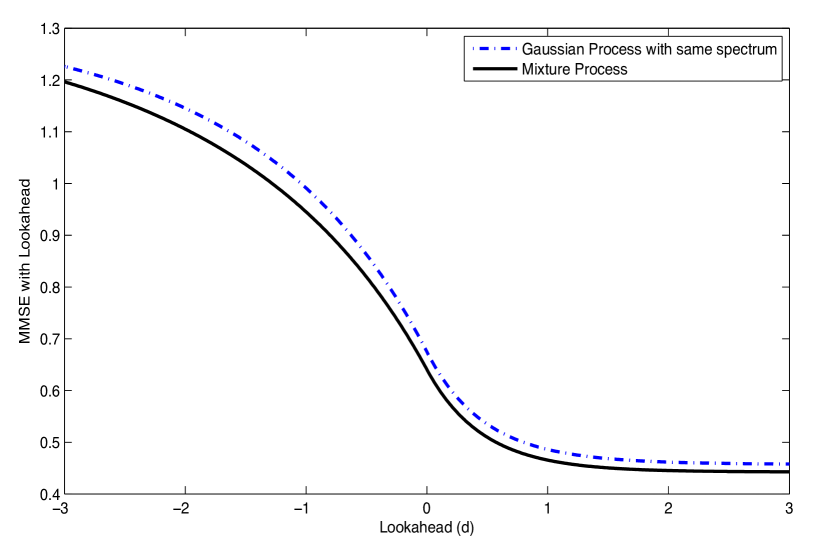
for all d𝑑d. Note that when d=βˆ’βˆžπ‘‘d=-\infty, the quantity lmmse​(βˆ’βˆž,snr)lmmsesnr{\text{lmmse}}(-\infty,{\text{snr}}) will be given by the stationary variance of the underlying process. Since this quantity depends only on the spectrum of the stationary process, the lower bound in (43) will coincide with the estimation error for the 𝐆𝐆\mathbf{G} process at d=βˆ’βˆžπ‘‘d=-\infty. For the 𝐆𝐆\mathbf{G} process, we can analytically compute the mmse with finite lookahead (124) as well, using the method outlined in Section IV-A. The reader is referred to Appendix B for a detailed discussion on computing the estimation error with finite lookahead for the 𝐆𝐆\mathbf{G} process under any Ξ±1,Ξ±2subscript𝛼1subscript𝛼2\alpha_{1},\alpha_{2}. For the purposes of this example, we illustrate the bound (43) for the case when Ξ±1=0.75subscript𝛼10.75\alpha_{1}=0.75 and Ξ±2=0.25subscript𝛼20.25\alpha_{2}=0.25. In Fig. 3, we present the mmse with lookahead for process 𝐆𝐆\mathbf{G}, as well as the lower bound, given by the corresponding quantity for 𝐗𝐗\mathbf{X}. For the given choice of parameters, at snr=1snr1{\text{snr}}=1: lmmse𝐗​(βˆ’βˆž,snr)=lmmse𝐆​(βˆ’βˆž,snr)=1.333subscriptlmmse𝐗snrsubscriptlmmse𝐆snr1.333{\text{lmmse}}_{\mathbf{X}}(-\infty,{\text{snr}})={\text{lmmse}}_{\mathbf{G}}(-\infty,{\text{snr}})=1.333; lmmse𝐗​(+∞,snr)=0.4425subscriptlmmse𝐗snr0.4425{\text{lmmse}}_{\mathbf{X}}(+\infty,{\text{snr}})=0.4425; lmmse𝐆​(+∞,snr)=0.4568subscriptlmmse𝐆snr0.4568{\text{lmmse}}_{\mathbf{G}}(+\infty,{\text{snr}})=0.4568.

Refer to caption
Figure 3: Illustration of the bound in (43). Plot of MMSE with lookahead for the processes 𝐆𝐆\mathbf{G} and 𝐗𝐗\mathbf{X} in Example III-A, for snr=1snr1{\text{snr}}=1. 𝐗𝐗\mathbf{X} is a mixture of two Ornstein-Ulhenbeck processes with parameters Ξ±1=0.75subscript𝛼10.75\alpha_{1}=0.75 and Ξ±2=0.25subscript𝛼20.25\alpha_{2}=0.25 respectively. 𝐆𝐆\mathbf{G} is a stationary Gaussian process with the same spectrum as 𝐗𝐗\mathbf{X}.

III-B Towards deriving an Upper Bound

Note that Lemma 7 gives us a computable lower bound for the mmse with lookahead for a Gaussian process G𝐺G whose spectrum can be expressed as a mixture of spectra of Ornstein-Ulhenbeck processes, under an appropriate mixture ΞΌπœ‡\mu.

Define, the mismatched mmse with lookahead for a filter that assumes the underlying process has law P(Ξ²)superscript𝑃𝛽P^{(\beta)} [Ornstein-Ulhenbeck process with parameter β𝛽\beta], whereas the true law of the process is P(Ξ±)superscript𝑃𝛼P^{(\alpha)}

lmmseΞ±,β​(d,Ξ³)=𝔼α​[(X0βˆ’π”ΌΞ²β€‹[X0|Yβˆ’βˆžd])2],subscriptlmmse𝛼𝛽𝑑𝛾subscript𝔼𝛼delimited-[]superscriptsubscript𝑋0subscript𝔼𝛽delimited-[]conditionalsubscript𝑋0superscriptsubscriptπ‘Œπ‘‘2\displaystyle{\text{lmmse}}_{\alpha,\beta}\,(d,\gamma)=\mathbb{E}_{\alpha}[(X_{0}-\mathbb{E}_{\beta}[X_{0}|Y_{-\infty}^{d}])^{2}], (52)

where the outer expectation is with respect to the true law of the underlying process P(Ξ±)superscript𝑃𝛼P^{(\alpha)}, while the inner expectation is with respect to the mismatched law P(Ξ²)superscript𝑃𝛽P^{(\beta)}. Note that the mismatched filter which assumes that the underlying signal is an Ornstein-Ulhenbeck process with parameter β𝛽\beta, is in particular, a linear filter. The process G𝐺G is Gaussian, and hence the optimal filter for G𝐺G is also linear. Thus, for any fixed β𝛽\beta, the mismatched filter thus defined, will be suboptimal for process G𝐺G. This yields the following natural upper bound, which in conjunction with Lemma 7 can be stated as:

Lemma 8 (Upper and lower bound in terms of mixture of Ornstein-Ulhenbeck spectra)
∫lmmseα​(d,Ξ³)​𝑑μ​(Ξ±)≀lmmseG​(d,Ξ³)≀minΞ²>0β€‹βˆ«lmmseΞ±,β​(d,Ξ³)​𝑑μ​(Ξ±).subscriptlmmse𝛼𝑑𝛾differential-dπœ‡π›Όsubscriptlmmse𝐺𝑑𝛾subscript𝛽0subscriptlmmse𝛼𝛽𝑑𝛾differential-dπœ‡π›Ό\displaystyle\int{\text{lmmse}}_{\alpha}(d,\gamma)\,d\mu(\alpha)\leq{\text{lmmse}}_{G}(d,\gamma)\leq\min_{\beta>0}\int{\text{lmmse}}_{\alpha,\beta}\,(d,\gamma)\,d\mu(\alpha). (53)

We should note that the upper bound stated in Lemma 8 can be hard to compute for continuous time processes, even though the filter applied is linear. In summary, analysis of lmmse​(β‹…,Ξ³)lmmse⋅𝛾{\text{lmmse}}(\cdot,\gamma) for the Ornstein-Uhlenbeck process provides us with a rich class of processes for which we can compute the finite lookahead estimation error. And for a class of Gaussian processes (45), we have a lower and upper bound on this quantity. These characterizations may be used to approximate the behavior of the MMSE with finite lookahead for a large class of Gaussian processes, instead of obtaining the optimal solution which relies on spectral factorization, and can be cumbersome.

IV Stationary Gaussian Processes

In this section, we focus exclusively on Gaussian processes having a known spectrum. We are interested in obtaining the MMSE with finite lookahead in estimating such a process when corrupted by AWGN at a fixed SNR level γ𝛾\gamma.

IV-A Calculation of MMSE with finite lookahead via Spectral Factorization

Let {Xt,tβˆˆβ„}subscript𝑋𝑑𝑑ℝ\{X_{t},t\in\mathbb{R}\} stationary and Gaussian, with power spectral density SX​(Ο‰)subscriptπ‘†π‘‹πœ”S_{X}(\omega), be the input to the continuous-time Gaussian channel at SNR γ𝛾\gamma. Y(β‹…)subscriptπ‘Œβ‹…Y_{(\cdot)}, the noise corrupted version of X(β‹…)subscript𝑋⋅X_{(\cdot)}, is stationary, Gaussian and has PSD SY​(Ο‰)=1+γ​SX​(Ο‰)subscriptπ‘†π‘Œπœ”1𝛾subscriptπ‘†π‘‹πœ”S_{Y}(\omega)=1+\gamma S_{X}(\omega). Let SY+​(Ο‰)superscriptsubscriptπ‘†π‘Œπœ”S_{Y}^{+}(\omega) be the Wiener-Hopf factorization of SY​(Ο‰)subscriptπ‘†π‘Œπœ”S_{Y}(\omega), i.e. a function satisfying |SY+​(Ο‰)|2=SY​(Ο‰)superscriptsuperscriptsubscriptπ‘†π‘Œπœ”2subscriptπ‘†π‘Œπœ”\left|S_{Y}^{+}(\omega)\right|^{2}=S_{Y}(\omega) with 1/SY+​(Ο‰)1superscriptsubscriptπ‘†π‘Œπœ”1/S_{Y}^{+}(\omega) being the transfer function of a stable causal filter. This factorization exists whenever the Paley-Wiener conditions are satisfied for SY​(Ο‰)subscriptπ‘†π‘Œπœ”S_{Y}(\omega). Denote by Y~tsubscript~π‘Œπ‘‘{\tilde{Y}}_{t} the output of the filter 1/SY+​(Ο‰)1superscriptsubscriptπ‘†π‘Œπœ”1/S_{Y}^{+}(\omega) applied on Ytsubscriptπ‘Œπ‘‘Y_{t}, then Y~tsubscript~π‘Œπ‘‘{\tilde{Y}}_{t} is a standard Brownian motion. This theory is well developed and the reader is encouraged to peruse any standard reference in continuous-time estimation for details (cf., e.g., [10] and references therein ).

Let h​(t)β„Žπ‘‘h(t) be the impulse response of the filter with transfer function

H​(Ο‰)=γ​SX​(Ο‰)SYβˆ’β€‹(Ο‰),π»πœ”π›Ύsubscriptπ‘†π‘‹πœ”superscriptsubscriptπ‘†π‘Œπœ”\displaystyle H(\omega)=\frac{\sqrt{\gamma}S_{X}(\omega)}{S_{Y}^{-}(\omega)}, (54)

with SYβˆ’β€‹(Ο‰)=SY+​(βˆ’Ο‰)superscriptsubscriptπ‘†π‘Œπœ”superscriptsubscriptπ‘†π‘Œπœ”S_{Y}^{-}(\omega)=S_{Y}^{+}(-\omega). The classical result by Wiener and Hopf [11], applied to non-causal filtering of stationary Gaussian signals can be stated as,

𝔼​[X0|Yβˆ’βˆžβˆž]=𝔼​[X0|Y~βˆ’βˆžβˆž]=βˆ«βˆ’βˆžβˆžh​(βˆ’t)​𝑑Y~t.𝔼delimited-[]conditionalsubscript𝑋0superscriptsubscriptπ‘Œπ”Όdelimited-[]conditionalsubscript𝑋0superscriptsubscript~π‘Œsuperscriptsubscriptβ„Žπ‘‘differential-dsubscript~π‘Œπ‘‘\displaystyle\mathbb{E}\left[X_{0}|Y_{-\infty}^{\infty}\right]=\mathbb{E}\left[X_{0}|\tilde{Y}_{-\infty}^{\infty}\right]=\int_{-\infty}^{\infty}h(-t)d\tilde{Y}_{t}. (55)

Moreover, an expression for the finite-lookahead MMSE estimator of X0subscript𝑋0X_{0} can be immediately derived, using the fact that Y~tsubscript~π‘Œπ‘‘{\tilde{Y}}_{t} is both a standard Brownian motion and a reversible causal function of the observations:

𝔼​[X0|Yβˆ’βˆžd]𝔼delimited-[]conditionalsubscript𝑋0superscriptsubscriptπ‘Œπ‘‘\displaystyle\mathbb{E}\left[X_{0}|Y_{-\infty}^{d}\right] =\displaystyle= 𝔼​[X0|Y~βˆ’βˆžd]=𝔼​[𝔼​{X0|Y~βˆ’βˆžβˆž}|Y~βˆ’βˆžd]𝔼delimited-[]conditionalsubscript𝑋0superscriptsubscript~π‘Œπ‘‘π”Όdelimited-[]conditional𝔼conditional-setsubscript𝑋0superscriptsubscript~π‘Œsuperscriptsubscript~π‘Œπ‘‘\displaystyle\mathbb{E}\left[X_{0}|\tilde{Y}_{-\infty}^{d}\right]=\mathbb{E}\left[\mathbb{E}\left\{X_{0}|\tilde{Y}_{-\infty}^{\infty}\right\}|\tilde{Y}_{-\infty}^{d}\right] (56)
=\displaystyle= 𝔼​[βˆ«βˆ’βˆžβˆžh​(βˆ’t)​𝑑Y~t|Y~βˆ’βˆžd]=βˆ«βˆ’βˆždh​(βˆ’t)​𝑑Y~t.𝔼delimited-[]conditionalsuperscriptsubscriptβ„Žπ‘‘differential-dsubscript~π‘Œπ‘‘superscriptsubscript~π‘Œπ‘‘superscriptsubscriptπ‘‘β„Žπ‘‘differential-dsubscript~π‘Œπ‘‘\displaystyle\mathbb{E}\left[\int_{-\infty}^{\infty}h(-t)d\tilde{Y}_{t}|\tilde{Y}_{-\infty}^{d}\right]=\int_{-\infty}^{d}h(-t)d\tilde{Y}_{t}. (57)

Using again the fact that Y~tsubscript~π‘Œπ‘‘{\tilde{Y}}_{t} is a brownian motion, as well as the orthogonality property of MMSE estimators, we can obtain a simple expression for lmmse​(d,Ξ³)lmmse𝑑𝛾\textrm{lmmse}(d,\gamma):

lmmse​(d,Ξ³)lmmse𝑑𝛾\displaystyle{\text{lmmse}}(d,\gamma) =\displaystyle= 𝔼​(X0βˆ’π”Όβ€‹[X0|Yβˆ’βˆžd])2=𝔼​(X0βˆ’π”Όβ€‹[X0|Y~βˆ’βˆžd])2𝔼superscriptsubscript𝑋0𝔼delimited-[]conditionalsubscript𝑋0superscriptsubscriptπ‘Œπ‘‘2𝔼superscriptsubscript𝑋0𝔼delimited-[]conditionalsubscript𝑋0superscriptsubscript~π‘Œπ‘‘2\displaystyle\mathbb{E}\left(X_{0}-\mathbb{E}\left[X_{0}|Y_{-\infty}^{d}\right]\right)^{2}=\mathbb{E}\left(X_{0}-\mathbb{E}\left[X_{0}|{\tilde{Y}}_{-\infty}^{d}\right]\right)^{2} (58)
=\displaystyle= 𝔼​(X0βˆ’π”Όβ€‹[X0|Y~βˆ’βˆžβˆž])2+𝔼​(𝔼​[X0|Y~βˆ’βˆžβˆž]βˆ’π”Όβ€‹[X0|Y~βˆ’βˆžd])2𝔼superscriptsubscript𝑋0𝔼delimited-[]conditionalsubscript𝑋0superscriptsubscript~π‘Œ2𝔼superscript𝔼delimited-[]conditionalsubscript𝑋0superscriptsubscript~π‘Œπ”Όdelimited-[]conditionalsubscript𝑋0superscriptsubscript~π‘Œπ‘‘2\displaystyle\mathbb{E}\left(X_{0}-\mathbb{E}\left[X_{0}|{\tilde{Y}}_{-\infty}^{\infty}\right]\right)^{2}+\mathbb{E}\left(\mathbb{E}\left[X_{0}|{\tilde{Y}}_{-\infty}^{\infty}\right]-\mathbb{E}\left[X_{0}|{\tilde{Y}}_{-\infty}^{d}\right]\right)^{2} (59)
=\displaystyle= mmse​(Ξ³)+𝔼​(∫d∞h​(βˆ’t)​𝑑Y~t)2=mmse​(Ξ³)+βˆ«βˆ’βˆžβˆ’dh2​(t)​𝑑t.mmse𝛾𝔼superscriptsuperscriptsubscriptπ‘‘β„Žπ‘‘differential-dsubscript~π‘Œπ‘‘2mmse𝛾superscriptsubscript𝑑superscriptβ„Ž2𝑑differential-d𝑑\displaystyle{\text{mmse}}(\gamma)+\mathbb{E}\left(\int_{d}^{\infty}h(-t)d\tilde{Y}_{t}\right)^{2}={\text{mmse}}(\gamma)+\int_{-\infty}^{-d}h^{2}(t)dt. (60)

This classical formulation of the lookahead problem for stationary Gaussian processes shows us that the MMSE with lookahead behaves gracefully with the lookahead d𝑑d, and is intimately connected to the impulse response h​(β‹…)β„Žβ‹…h(\cdot) of the filter induced by the Wiener spectral factorization process. In particular, that the solution to the lookahead problem for each value of d𝑑d, can be approached in this single unified manner as shown in (60), is quite satisfying.

IV-B Processes with a rational spectrum

Let SX​(Ο‰)subscriptπ‘†π‘‹πœ”S_{X}(\omega) be a rational function, i.e. of the form P​(Ο‰)Q​(Ο‰)π‘ƒπœ”π‘„πœ”\frac{P(\omega)}{Q(\omega)} with P,Q𝑃𝑄P,Q being finite order polynomials in Ο‰πœ”\omega. In this case SY​(Ο‰)subscriptπ‘†π‘Œπœ”S_{Y}(\omega) is also a rational function, and the Wiener-Hopf factorization can be preformed simply by factorizing the numerator and denominator of SY​(Ο‰)subscriptπ‘†π‘Œπœ”S_{Y}(\omega) and composing SY+​(Ο‰)subscriptsuperscriptπ‘†π‘Œπœ”S^{+}_{Y}(\omega) only from the stable zeros and poles.

Recall the definition of pdsubscript𝑝𝑑p_{d} in (34),

pd≐lmmse​(d,Ξ³)βˆ’mmse​(Ξ³)cmmse​(Ξ³)βˆ’mmse​(Ξ³).approaches-limitsubscript𝑝𝑑lmmse𝑑𝛾mmse𝛾cmmse𝛾mmse𝛾\displaystyle p_{d}\doteq\frac{{\text{lmmse}}(d,\gamma)-{\text{mmse}}(\gamma)}{{\text{cmmse}}(\gamma)-{\text{mmse}}(\gamma)}. (61)

Clearly, p0=1subscript𝑝01p_{0}=1 and limdβ†’βˆžpd=0subscript→𝑑subscript𝑝𝑑0\lim_{d{\rightarrow}\infty}p_{d}=0. The value pdsubscript𝑝𝑑p_{d} goes to zero in the same rate as lmmse converges to mmse. For the Ornstein-Ulhenbeck process we observed that pdsubscript𝑝𝑑p_{d} converges exponentially to zero. In the following lemma, we generalize this result to include all Gaussian input processes with rational spectra

Lemma 9

For any Gaussian input process with a rational spectrum, lmmse​(d,snr)lmmse𝑑snr{\text{lmmse}}(d,{\text{snr}}) approaches mmse​(snr)mmsesnr{\text{mmse}}({\text{snr}}) exponentially fast as dβ†’βˆžβ†’π‘‘d{\rightarrow}\infty. Equivalently, pdβ†’0β†’subscript𝑝𝑑0p_{d}\to 0 exponentially, as dβ†’βˆžβ†’π‘‘d\to\infty.

Proof:

Since SY+​(Ο‰)subscriptsuperscriptπ‘†π‘Œπœ”S^{+}_{Y}(\omega) is a rational function, so is H​(Ο‰)π»πœ”H(\omega) defined in (54). Therefore, h​(t)β„Žπ‘‘h(t) must be a finite sum of exponentially decreasing functions [should use a ref here] and consequently βˆ«βˆ’βˆžβˆ’dh2​(t)​𝑑tsuperscriptsubscript𝑑superscriptβ„Ž2𝑑differential-d𝑑\int_{-\infty}^{-d}h^{2}(t)dt must also decrease exponentially as dβ†’βˆžβ†’π‘‘d{\rightarrow}\infty. This in conjunction with the relation in (60) concludes the proof. ∎

As an illustration, we consider an equal mixture of two Ornstein-Ulhenbeck processes with parameters Ξ±1subscript𝛼1\alpha_{1} and Ξ±2subscript𝛼2\alpha_{2}, as in the example of the previous section. In Appendix B the mmse with lookahead is explicitly computed for a Gaussian process with this spectrum, acting as input to the channel. From these calculations, one can observe that the corresponding expression for pdsubscript𝑝𝑑p_{d} in (127) vanishes exponentially with increasing lookahead. However, it is important to note that there exist input spectra for which the decay of pdsubscript𝑝𝑑p_{d} is not exponentially fast.

As an example, consider the input power spectrum

SXtriang​(Ο‰)=(1βˆ’|Ο‰|)β€‹πŸ{|Ο‰|≀1},subscriptsuperscript𝑆triangπ‘‹πœ”1πœ”subscript1πœ”1\displaystyle S^{\text{triang}}_{X}(\omega)=\left(1-|\omega|\right)\mathbf{1}_{\left\{\left|\omega\right|\leq 1\right\}}, (62)

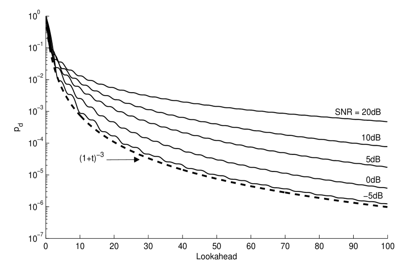
and In Figure 4 we plot the behaviour of pdsubscript𝑝𝑑p_{d} as a function of d𝑑d for input power spectrum SXtriang​(Ο‰)subscriptsuperscript𝑆triangπ‘‹πœ”S^{\text{triang}}_{X}(\omega) and different SNR’s. This demonstrates the polynomial rate of convergence of the finite lookahead estimation error towards to non-causal MMSE. The values of lmmse​(d,snr)lmmse𝑑snr{\text{lmmse}}(d,{\text{snr}}) were found by numerically approximating h​(t)β„Žπ‘‘h(t), using FFT in order to perform the factorization of SY​(Ο‰)subscriptπ‘†π‘Œπœ”S_{Y}(\omega).

Refer to caption
Figure 4: Plot of pdsubscript𝑝𝑑p_{d} as defined in (34), vs. lookahead in various SNRs, for input power spectrum (1βˆ’|Ο‰|)β€‹πŸ{|Ο‰|≀1}1πœ”subscript1πœ”1\left(1-|\omega|\right)\mathbf{1}_{\left\{\left|\omega\right|\leq 1\right\}}. The finite lookahead MMSE is seen to converge to the non-causal MMSE at an approximately cubic rate.

V Information Utility Of Lookahead

Consider a stationary process Xtsubscript𝑋𝑑X_{t} observed through the continuous-time Gaussian channel (1) at SNR level γ𝛾\gamma. In the previous sections we have tried to ascertain the benefit of lookahead in mean squared estimation. We now address the question, how much information does lookahead provide in general, and whether this quantity has any interesting connections with classical estimation theoretic objects.

For Ο„>0𝜏0\tau>0, let us define the Information Utility U​(β‹…)π‘ˆβ‹…U(\cdot) as a function of lookahead Ο„πœ\tau, to be

U​(Ο„)=I​(X0;Y0Ο„|Yβˆ’βˆž0).π‘ˆπœπΌsubscript𝑋0conditionalsuperscriptsubscriptπ‘Œ0𝜏superscriptsubscriptπ‘Œ0\displaystyle U(\tau)=I(X_{0};Y_{0}^{\tau}|Y_{-\infty}^{0}). (63)

When the input process is Gaussian,

U​(Ο„)π‘ˆπœ\displaystyle U(\tau) =\displaystyle= h​(X0|Yβˆ’βˆž0)βˆ’h​(X0|Yβˆ’βˆžΟ„)=12​log⁑(2​π​e​Var​(X0|Yβˆ’βˆž0))βˆ’12​log⁑(2​π​e​Var​(X0|Yβˆ’βˆžΟ„))β„Žconditionalsubscript𝑋0superscriptsubscriptπ‘Œ0β„Žconditionalsubscript𝑋0superscriptsubscriptπ‘Œπœ122πœ‹π‘’Varconditionalsubscript𝑋0superscriptsubscriptπ‘Œ0122πœ‹π‘’Varconditionalsubscript𝑋0superscriptsubscriptπ‘Œπœ\displaystyle h(X_{0}|Y_{-\infty}^{0})-h(X_{0}|Y_{-\infty}^{\tau})=\frac{1}{2}\log\left(2{\pi}e{\text{Var}}(X_{0}|Y_{-\infty}^{0})\right)-\frac{1}{2}\log\left(2{\pi}e{\text{Var}}(X_{0}|Y_{-\infty}^{\tau})\right) (64)
=\displaystyle= 12​log⁑(cmmse​(snr)lmmse​(Ο„,snr)).12cmmsesnrlmmse𝜏snr\displaystyle\frac{1}{2}\log\left(\frac{{\text{cmmse}}({\text{snr}})}{{\text{lmmse}}(\tau,{\text{snr}})}\right). (65)

Rearranging the terms, we have

lmmse​(Ο„,snr)=cmmse​(snr)​exp⁑(βˆ’2​U​(Ο„)).lmmse𝜏snrcmmsesnr2π‘ˆπœ\displaystyle{\text{lmmse}}(\tau,{\text{snr}})={\text{cmmse}}({\text{snr}})\exp({-2U(\tau)}). (66)

Furthermore, when the input is non-Gaussian but h​(X0|Yβˆ’βˆžΟ„)β„Žconditionalsubscript𝑋0superscriptsubscriptπ‘Œπœh(X_{0}|Y_{-\infty}^{\tau}) is well-defined for every Ο„β‰₯0𝜏0\tau\geq 0,

h​(X0|Yβˆ’βˆžΟ„)≀𝔼yβˆ’βˆžΟ„β€‹[12​log⁑(2​π​e​Var​(X0|Yβˆ’βˆžΟ„=yβˆ’βˆžΟ„))]≀12​log⁑(2​π​e​lmmse​(Ο„,snr)).β„Žconditionalsubscript𝑋0superscriptsubscriptπ‘Œπœsubscript𝔼superscriptsubscriptπ‘¦πœdelimited-[]122πœ‹π‘’Varconditionalsubscript𝑋0superscriptsubscriptπ‘Œπœsuperscriptsubscriptπ‘¦πœ122πœ‹π‘’lmmse𝜏snr\displaystyle h(X_{0}|Y_{-\infty}^{\tau})\leq\mathbb{E}_{y_{-\infty}^{\tau}}\left[\frac{1}{2}\log\left(2{\pi}e{\text{Var}}(X_{0}|Y_{-\infty}^{\tau}=y_{-\infty}^{\tau})\right)\right]\leq\frac{1}{2}\log\left(2{\pi}e{\text{lmmse}}(\tau,{\text{snr}})\right). (67)

The first inequality is due to the fact that the Gaussian distribution has maximum entropy under a variance constraint, and the second inequality follows from Jensen’s inequality. Rearranging the terms once more, we have that for every stationary input process,

lmmse​(Ο„,snr)β‰₯N​(X0|Yβˆ’βˆž0)​exp⁑(βˆ’2​U​(Ο„)),lmmse𝜏snr𝑁conditionalsubscript𝑋0superscriptsubscriptπ‘Œ02π‘ˆπœ\displaystyle{\text{lmmse}}(\tau,{\text{snr}}){\geq}N(X_{0}|Y_{-\infty}^{0})\exp({-2U(\tau)}), (68)

where N​(Z)=12​π​e​exp⁑(2​h​(Z))𝑁𝑍12πœ‹π‘’2β„Žπ‘N(Z)=\frac{1}{2{\pi}e}\exp({2h(Z)}) is the entropy power functional.

We now present a relation between U​(β‹…)π‘ˆβ‹…U(\cdot) and the MMSE via a differential equation. Consider an infinitesimal increment dβ€‹Ο„π‘‘πœd\tau in U​(Ο„)π‘ˆπœU(\tau),

U​(Ο„+d​τ)βˆ’U​(Ο„)=I​(X0;Yττ+d​τ|Yβˆ’βˆžΟ„)=I​(Xττ+d​τ;Yττ+d​τ|Yβˆ’βˆžΟ„)βˆ’I​(Xττ+d​τ;Yττ+d​τ|Yβˆ’βˆžΟ„,X0).π‘ˆπœπ‘‘πœπ‘ˆπœπΌsubscript𝑋0conditionalsuperscriptsubscriptπ‘Œπœπœπ‘‘πœsuperscriptsubscriptπ‘ŒπœπΌsuperscriptsubscriptπ‘‹πœπœπ‘‘πœconditionalsuperscriptsubscriptπ‘Œπœπœπ‘‘πœsuperscriptsubscriptπ‘ŒπœπΌsuperscriptsubscriptπ‘‹πœπœπ‘‘πœconditionalsuperscriptsubscriptπ‘Œπœπœπ‘‘πœsuperscriptsubscriptπ‘Œπœsubscript𝑋0\displaystyle U(\tau+d\tau)-U(\tau)=I(X_{0};Y_{\tau}^{\tau+d\tau}|Y_{-\infty}^{\tau})=I(X_{\tau}^{\tau+d\tau};Y_{\tau}^{\tau+d\tau}|Y_{-\infty}^{\tau})-I(X_{\tau}^{\tau+d\tau};Y_{\tau}^{\tau+d\tau}|Y_{-\infty}^{\tau},X_{0}). (69)

The last equality is due to the Markov Chain relationship X0βˆ’(Xττ+d​τ,Yβˆ’βˆžΟ„)βˆ’Yττ+d​τsubscript𝑋0superscriptsubscriptπ‘‹πœπœπ‘‘πœsuperscriptsubscriptπ‘Œπœsuperscriptsubscriptπ‘Œπœπœπ‘‘πœX_{0}-(X_{\tau}^{\tau+\,d\tau},Y_{-\infty}^{\tau})-Y_{\tau}^{\tau+d\tau}. Using the time-incremental channel argument introduced in [2, Section III.D], we are able to write,

I​(Xττ+d​τ;Yττ+d​τ|Yβˆ’βˆžΟ„)=12​d​τ⋅snrβ‹…Var​(XΟ„|Yβˆ’βˆžΟ„)+o​(d​τ),𝐼superscriptsubscriptπ‘‹πœπœπ‘‘πœconditionalsuperscriptsubscriptπ‘Œπœπœπ‘‘πœsuperscriptsubscriptπ‘Œπœβ‹…12π‘‘πœsnrVarconditionalsubscriptπ‘‹πœsuperscriptsubscriptπ‘Œπœπ‘œπ‘‘πœ\displaystyle I(X_{\tau}^{\tau+d\tau};Y_{\tau}^{\tau+d\tau}|Y_{-\infty}^{\tau})=\frac{1}{2}\,d\tau\cdot{{\text{snr}}}{\cdot}{\text{Var}}(X_{\tau}|Y_{-\infty}^{\tau})+o(d\tau), (70)

and

I​(Xττ+d​τ;Yττ+d​τ|Yβˆ’βˆžΟ„,X0)=12​d​τ⋅snrβ‹…Var​(XΟ„|Yβˆ’βˆžΟ„,X0)+o​(d​τ).𝐼superscriptsubscriptπ‘‹πœπœπ‘‘πœconditionalsuperscriptsubscriptπ‘Œπœπœπ‘‘πœsuperscriptsubscriptπ‘Œπœsubscript𝑋0β‹…12π‘‘πœsnrVarconditionalsubscriptπ‘‹πœsuperscriptsubscriptπ‘Œπœsubscript𝑋0π‘œπ‘‘πœ\displaystyle I(X_{\tau}^{\tau+d\tau};Y_{\tau}^{\tau+d\tau}|Y_{-\infty}^{\tau},X_{0})=\frac{1}{2}\,d\tau{\cdot}{{\text{snr}}}{\cdot}{\text{Var}}(X_{\tau}|Y_{-\infty}^{\tau},X_{0})+o(d\tau). (71)

The expression for the time derivative of the information utility function is therefore,

U′​(Ο„)=snr2​(Var​(XΟ„|Yβˆ’βˆžΟ„)βˆ’Var​(XΟ„|Yβˆ’βˆžΟ„,X0)).superscriptπ‘ˆβ€²πœsnr2Varconditionalsubscriptπ‘‹πœsuperscriptsubscriptπ‘ŒπœVarconditionalsubscriptπ‘‹πœsuperscriptsubscriptπ‘Œπœsubscript𝑋0\displaystyle U^{\prime}(\tau)=\frac{{\text{snr}}}{2}\left({\text{Var}}(X_{\tau}|Y_{-\infty}^{\tau})-{\text{Var}}(X_{\tau}|Y_{-\infty}^{\tau},X_{0})\right). (72)

Since the input is assumed stationary, Var​(XΟ„|Yβˆ’βˆžΟ„)=Var​(X0|Yβˆ’βˆž0)=cmmse​(snr)Varconditionalsubscriptπ‘‹πœsuperscriptsubscriptπ‘ŒπœVarconditionalsubscript𝑋0superscriptsubscriptπ‘Œ0cmmsesnr{\text{Var}}(X_{\tau}|Y_{-\infty}^{\tau})={\text{Var}}(X_{0}|Y_{-\infty}^{0})={\text{cmmse}}({\text{snr}}). We notice that Var​(XΟ„|Yβˆ’βˆžΟ„,X0)Varconditionalsubscriptπ‘‹πœsuperscriptsubscriptπ‘Œπœsubscript𝑋0{\text{Var}}(X_{\tau}|Y_{-\infty}^{\tau},X_{0}) is the causal MMSE in estimating XΟ„subscriptπ‘‹πœX_{\tau} when X0subscript𝑋0X_{0} is known. The value of U′​(Ο„)superscriptπ‘ˆβ€²πœU^{\prime}(\tau) is therefore intimately connected to the effect of initial conditions on the causal MMSE estimation of the process. In particular,

U′​(0)=snr2​cmmse​(snr),superscriptπ‘ˆβ€²0snr2cmmsesnr\displaystyle U^{\prime}(0)=\frac{{\text{snr}}}{2}{\text{cmmse}}({\text{snr}}), (73)

meaning that the added value in information of an infinitesimal lookahead is proportional to the causal MMSE.

Noticing that U​(0)=0π‘ˆ00U(0)=0, we may integrate (72) to obtain,

U​(Ο„)=snr2​[τ​cmmse​(snr)βˆ’βˆ«0Ο„Var​(Xs|Yβˆ’βˆžs,X0)​𝑑s].π‘ˆπœsnr2delimited-[]𝜏cmmsesnrsuperscriptsubscript0𝜏Varconditionalsubscript𝑋𝑠superscriptsubscriptπ‘Œπ‘ subscript𝑋0differential-d𝑠\displaystyle U(\tau)=\frac{{\text{snr}}}{2}\left[\tau\,{\text{cmmse}}({\text{snr}})-\int_{0}^{\tau}{\text{Var}}(X_{s}|Y_{-\infty}^{s},X_{0})\,ds\right]. (74)

Specializing to stationary Gaussian input processes, and joining equations (66) and (74), we obtain

lmmse​(Ο„,snr)=cmmse​(snr)​exp⁑[βˆ’snr​(τ​cmmse​(snr)βˆ’βˆ«0Ο„Var​(Xs|Yβˆ’βˆžs,X0)​𝑑s)].lmmse𝜏snrcmmsesnrsnr𝜏cmmsesnrsuperscriptsubscript0𝜏Varconditionalsubscript𝑋𝑠superscriptsubscriptπ‘Œπ‘ subscript𝑋0differential-d𝑠\displaystyle{\text{lmmse}}(\tau,{\text{snr}})={\text{cmmse}}({\text{snr}})\exp{\left[-{\text{snr}}\left(\tau{\text{cmmse}}({\text{snr}})-\int_{0}^{\tau}{\text{Var}}(X_{s}|Y_{-\infty}^{s},X_{0})\,ds\right)\right]}. (75)

For the Ornstein-Uhlenbeck process, Var​(Xs|Yβˆ’βˆžs,X0)Varconditionalsubscript𝑋𝑠superscriptsubscriptπ‘Œπ‘ subscript𝑋0{\text{Var}}(X_{s}|Y_{-\infty}^{s},X_{0}) can be calculated explicitly. This, in conjunction with (75), provides an alternative derivation of the finite lookahead MMSE in the Ornstein-Uhlenbeck process, that is based on Information-Estimation arguments. The reader is referred to Appendix C for more details.

VI Generalized Observation Model

In this section, we present a new observation model to understand the behavior of estimation error with lookahead. Consider a stationary continuous-time stochastic process Xtsubscript𝑋𝑑X_{t}. The observation model is still additive Gaussian noise, where the SNR level of the channel has a jump at t=0𝑑0t=0. Letting Ytsubscriptπ‘Œπ‘‘Y_{t} denote the channel output, we describe the channel as given below.

d​Yt𝑑subscriptπ‘Œπ‘‘\displaystyle\,dY_{t} =\displaystyle= {snr​Xt​d​t+d​Wtt ≀ 0γ​Xt​d​t+d​WttΒ >Β 0casessnrsubscript𝑋𝑑𝑑𝑑𝑑subscriptπ‘Šπ‘‘t ≀ 0𝛾subscript𝑋𝑑𝑑𝑑𝑑subscriptπ‘Šπ‘‘tΒ >Β 0\displaystyle\left\{\begin{array}[]{l l}\sqrt{{\text{snr}}}\,X_{t}\,dt+\,dW_{t}&\quad\text{t $\leq$ 0}\\ \sqrt{\gamma}\,X_{t}\,dt+\,dW_{t}&\quad\text{t $>$ 0}\\ \end{array}\right. (78)

where, as usual, Wβ‹…subscriptπ‘Šβ‹…W_{\cdot} is a standard Brownian motion independent of 𝐗𝐗\mathbf{X}. Note that for Ξ³β‰ snr𝛾snr\gamma\neq{\text{snr}}, the (Xt,Yt)subscript𝑋𝑑subscriptπ‘Œπ‘‘(X_{t},Y_{t}) process is not jointly stationary. Letting d,lβ‰₯0𝑑𝑙0d,l\geq 0, we define the finite lookahead estimation error at time d𝑑d with lookahead l𝑙l as

f​(snr,Ξ³,d,l)𝑓snr𝛾𝑑𝑙\displaystyle f({\text{snr}},\gamma,d,l) =\displaystyle= Var​(Xd|Yβˆ’βˆžl+d).Varconditionalsubscript𝑋𝑑superscriptsubscriptπ‘Œπ‘™π‘‘\displaystyle{\text{Var}}(X_{d}|Y_{-\infty}^{l+d}). (79)

We call this a generalized observation model, as for Ξ³=snr𝛾snr\gamma={\text{snr}}, we recover the usual time-invariant Gaussian channel. For instance, we note that the error f𝑓f reduces to the filtering, smoothing or finite lookahead errors, depending on the parameters γ𝛾\gamma, l𝑙l and d𝑑d as:

cmmse​(snr)cmmsesnr\displaystyle{\text{cmmse}}({\text{snr}}) =f​(snr,snr,d,0)absent𝑓snrsnr𝑑0\displaystyle=f({\text{snr}},{\text{snr}},d,0) (80)
mmse​(snr)mmsesnr\displaystyle{\text{mmse}}({\text{snr}}) =f​(snr,snr,d,∞)absent𝑓snrsnr𝑑\displaystyle=f({\text{snr}},{\text{snr}},d,\infty) (81)
lmmse​(l,snr)lmmse𝑙snr\displaystyle{\text{lmmse}}(l,{\text{snr}}) =f​(snr,snr,t,l)absent𝑓snrsnr𝑑𝑙\displaystyle=f({\text{snr}},{\text{snr}},t,l) (82)

In the following we relate the estimation error with finite lookahead for the observation model described in (78), with the original filtering error.

Theorem 10

Let Xtsubscript𝑋𝑑X_{t} be any finite variance continuous time stationary process which is corrupted by the Gaussian channel in (78). Let f𝑓f be as defined in (79). For fixed snr>0snr0{\text{snr}}>0 and T>0𝑇0T>0 let ΓΓ\Gamma ∼U​[0,snr]similar-toabsentπ‘ˆ0snr\sim U[0,{\text{snr}}] and L𝐿L ∼U​[0,T]similar-toabsentπ‘ˆ0𝑇\sim U[0,T] be independent random variables. Then

cmmse​(snr)=𝔼Γ,L​[f​(snr,Ξ“,Tβˆ’L,L)]cmmsesnrsubscript𝔼Γ𝐿delimited-[]𝑓snrΓ𝑇𝐿𝐿\displaystyle{\text{cmmse}}({\text{snr}})=\mathbb{E}_{\Gamma,L}[f({\text{snr}},\Gamma,T-L,L)] (83)
Proof:

Before proving this result, we take a detour to consider a stationary continuous-time stochastic process X0Tsuperscriptsubscript𝑋0𝑇X_{0}^{T} which is governed according to law PX0Tsubscript𝑃superscriptsubscript𝑋0𝑇P_{X_{0}^{T}} and is observed in the window t∈[0,T]𝑑0𝑇t\in[0,T] through the continuous-time Gaussian channel (1) at SNR level snr. We define the operators which evaluate the filtering and smoothing estimation errors for this process model, as follows:

cmmse¯​(PXT,snr)=∫0T𝔼​[(Xtβˆ’π”Όβ€‹[Xt|Yt])2]​𝑑tΒ―cmmsesubscript𝑃superscript𝑋𝑇snrsuperscriptsubscript0𝑇𝔼delimited-[]superscriptsubscript𝑋𝑑𝔼delimited-[]conditionalsubscript𝑋𝑑superscriptπ‘Œπ‘‘2differential-d𝑑\displaystyle\underline{{\text{cmmse}}}(P_{X^{T}},{\text{snr}})=\int_{0}^{T}\mathbb{E}[(X_{t}-\mathbb{E}[X_{t}|Y^{t}])^{2}]\,dt (84)
mmse¯​(PXT,snr)=∫0T𝔼​[(Xtβˆ’π”Όβ€‹[Xt|YT])2]​𝑑tΒ―mmsesubscript𝑃superscript𝑋𝑇snrsuperscriptsubscript0𝑇𝔼delimited-[]superscriptsubscript𝑋𝑑𝔼delimited-[]conditionalsubscript𝑋𝑑superscriptπ‘Œπ‘‡2differential-d𝑑\displaystyle\underline{{\text{mmse}}}(P_{X^{T}},{\text{snr}})=\int_{0}^{T}\mathbb{E}[(X_{t}-\mathbb{E}[X_{t}|Y^{T}])^{2}]\,dt (85)

Further, [2] gives us the celebrated relationship between the causal and non-causal estimation errors:

cmmse¯​(PXT,snr)Β―cmmsesubscript𝑃superscript𝑋𝑇snr\displaystyle\underline{{\text{cmmse}}}(P_{X^{T}},{\text{snr}}) =\displaystyle= 1snrβ€‹βˆ«0snrmmse¯​(PXT,Ξ³)​𝑑γ.1snrsuperscriptsubscript0snrΒ―mmsesubscript𝑃superscript𝑋𝑇𝛾differential-d𝛾\displaystyle\frac{1}{{\text{snr}}}\int_{0}^{{\text{snr}}}\underline{{\text{mmse}}}(P_{X^{T}},\gamma)\,d\gamma. (86)

We now return to the auxiliary observation model introduced above. We note that the causal and non-causal estimation errors of process Xtsubscript𝑋𝑑X_{t} at signal to noise ratio snr, can be written in terms of

cmmse​(snr)cmmsesnr\displaystyle{\text{cmmse}}({\text{snr}}) =\displaystyle= 1T​𝔼snr​[cmmse¯​(PX0T|Yβˆ’βˆž0,snr)]1𝑇subscript𝔼snrdelimited-[]Β―cmmsesubscript𝑃conditionalsuperscriptsubscript𝑋0𝑇superscriptsubscriptπ‘Œ0snr\displaystyle\frac{1}{T}\mathbb{E}_{{\text{snr}}}\bigg{[}\underline{{\text{cmmse}}}(P_{X_{0}^{T}|Y_{-\infty}^{0}},{\text{snr}})\bigg{]} (87)
mmse​(snr)mmsesnr\displaystyle{\text{mmse}}({\text{snr}}) =\displaystyle= 1T​𝔼snr​[mmse¯​(PX0T|Yβˆ’βˆž0,snr)],1𝑇subscript𝔼snrdelimited-[]Β―mmsesubscript𝑃conditionalsuperscriptsubscript𝑋0𝑇superscriptsubscriptπ‘Œ0snr\displaystyle\frac{1}{T}\mathbb{E}_{{\text{snr}}}\bigg{[}\underline{{\text{mmse}}}(P_{X_{0}^{T}|Y_{-\infty}^{0}},{\text{snr}})\bigg{]}, (88)

where 𝔼snrsubscript𝔼snr\mathbb{E}_{{\text{snr}}} denotes expectation over Yβˆ’βˆž0superscriptsubscriptπ‘Œ0Y_{-\infty}^{0}. And, now employing the relation between the two quantities above, we get

1T​𝔼snr​[cmmse¯​(PX0T|Yβˆ’βˆž0,snr)]=1T​𝔼snr​[1snrβ€‹βˆ«0snrmmse¯​(PX0T|Yβˆ’βˆž0,Ξ³)​𝑑γ]1𝑇subscript𝔼snrdelimited-[]Β―cmmsesubscript𝑃conditionalsuperscriptsubscript𝑋0𝑇superscriptsubscriptπ‘Œ0snr1𝑇subscript𝔼snrdelimited-[]1snrsuperscriptsubscript0snrΒ―mmsesubscript𝑃conditionalsuperscriptsubscript𝑋0𝑇superscriptsubscriptπ‘Œ0𝛾differential-d𝛾\displaystyle\frac{1}{T}\mathbb{E}_{{\text{snr}}}\bigg{[}\underline{{\text{cmmse}}}(P_{X_{0}^{T}|Y_{-\infty}^{0}},{\text{snr}})\bigg{]}=\frac{1}{T}\mathbb{E}_{{\text{snr}}}\bigg{[}\frac{1}{{\text{snr}}}\int_{0}^{{\text{snr}}}\underline{{\text{mmse}}}(P_{X_{0}^{T}|Y_{-\infty}^{0}},\gamma)\,d\gamma\bigg{]} (89)

Using the definition of f𝑓f and inserting in above, we get the following intergral equation which holds for every stationary process Xtsubscript𝑋𝑑X_{t} observed through the continuous Gaussian channel as described in (78)

f​(snr,snr,x,0)=1Tβ‹…snrβ€‹βˆ«0snr∫0Tf​(snr,Ξ³,t,Tβˆ’t)​𝑑t​𝑑γ,𝑓snrsnrπ‘₯01⋅𝑇snrsuperscriptsubscript0snrsuperscriptsubscript0𝑇𝑓snr𝛾𝑑𝑇𝑑differential-d𝑑differential-d𝛾\displaystyle f({\text{snr}},{\text{snr}},x,0)=\frac{1}{T\cdot{\text{snr}}}\int_{0}^{{\text{snr}}}\int_{0}^{T}f({\text{snr}},\gamma,t,T-t)\,dt\,d\gamma, (90)

for all T and x. Note that the left hand side of (90) is nothing but the causal squared error at SNR level snr. Note, in particular, that for independent random variables ΓΓ\Gamma ∼U​[0,snr]similar-toabsentπ‘ˆ0snr\sim U[0,{\text{snr}}] and L𝐿L ∼U​[0,T]similar-toabsentπ‘ˆ0𝑇\sim U[0,T], (90) can be expressed as

cmmse​(snr)=𝔼Γ,L​[f​(snr,Ξ“,Tβˆ’L,L)].cmmsesnrsubscript𝔼Γ𝐿delimited-[]𝑓snrΓ𝑇𝐿𝐿\displaystyle{\text{cmmse}}({\text{snr}})=\mathbb{E}_{\Gamma,L}[f({\text{snr}},\Gamma,T-L,L)]. (91)

∎

Refer to caption
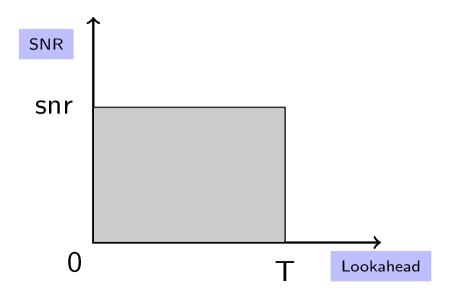
Figure 5: Region in the Lookahead-SNR plane over which the finite lookahead MMSE given by (79) is averaged over in Theorem 10 to yield the filtering error at level snr.

It is interesting to note that the double integral over lookahead and SNR are conserved in such a manner by the filtering error, for any arbitrary underlying stationary process. Note that one way of interpreting this result, is to take the average of the finite lookahead mmse (under the given observation model), over a rectangular region in the Lookahead vs. Signal-to-Noise Ratio plane, as depicted in Fig. 5. Theorem 10 tells us that for all underlying processes, this quantity is always the filtering error at level snr. Thus, we find the classical estimation theoretic quantity described by the causal error to emerge as a bridge between the effects of varying lookahead and the signal to noise ratio.

Given Theorem 10, it is natural to investigate whether the relation (83) can be inverted to determine the function f𝑓f, from the causal mmse. If that were the case, then, in particular, the filtering error would completely determine the estimation loss with finite lookahead. To pose an equivalent question, let us recall Duncan’s result in [1] establishing the equivalence of the mutual information rate and the filtering error. On the other hand, by [2, 15] the mutual information rate function I​(β‹…)𝐼⋅I(\cdot), determines the non-causal mmse. Might the same mutual information rate function I​(snr)𝐼snrI({\text{snr}}) can completely determine the estimation loss for a fixed finite lookahead d𝑑d as well ? This question is addressed in the following section.

VII Can I(β‹…β‹…\cdot) recover finite-lookahead mmse ?

Refer to caption
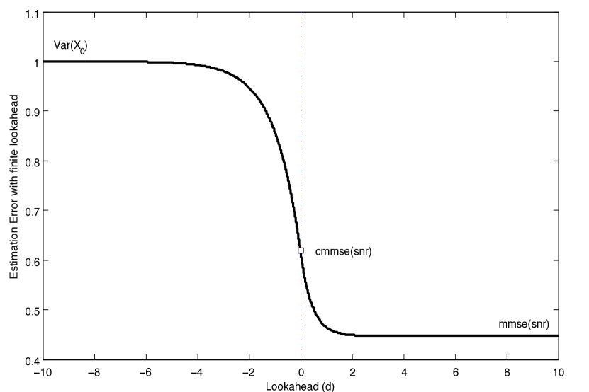
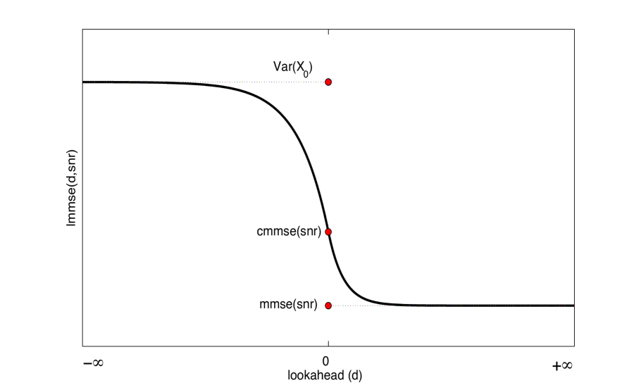
Figure 6: Characteristic behavior of the minimum mean squared error with lookahead for any process.

In Fig. 6, we present a characteristic plot of the mmse with lookahead for an arbitrary continuous time stationary process, corrupted by the Gaussian channel (1) at SNR level snr. In particular, we note three important features of the process, namely (i) the asymptote at d=βˆžπ‘‘d=\infty is mmse​(snr)mmsesnr{\text{mmse}}({\text{snr}}), (ii) lmmse​(0,snr)=cmmse​(snr)lmmse0snrcmmsesnr{\text{lmmse}}(0,{\text{snr}})={\text{cmmse}}({\text{snr}}) and (iii) the asymptote at d=βˆ’βˆžπ‘‘d=-\infty is the variance of the stationary process, Var​(X0)Varsubscript𝑋0{\text{Var}}(X_{0}). Further, the curve is non-decreasing for all d𝑑d.

From [1] and [2], we know that the mutual information, the causal, and the non-causal mmse determine each other according to

2​I​(snr)snr=cmmse​(snr)=1snrβ€‹βˆ«0snrmmse​(Ξ³)​𝑑γ.2𝐼snrsnrcmmsesnr1snrsuperscriptsubscript0snrmmse𝛾differential-d𝛾\displaystyle\frac{2I({\text{snr}})}{{\text{snr}}}={\text{cmmse}}({\text{snr}})=\frac{1}{{\text{snr}}}\int_{0}^{{\text{snr}}}{\text{mmse}}(\gamma)\,d\gamma. (92)

In other words, the mutual information rate function is sufficient to characterize the behavior of the causal and smoothing errors as functions of snr. In particular, (92) also determines the three important features of the lmmse​(β‹…,snr)lmmseβ‹…snr{\text{lmmse}}(\cdot,{\text{snr}}) curve discussed above, i.e. the value 333Note that Var​(X0)=cmmse​(0)Varsubscript𝑋0cmmse0{\text{Var}}(X_{0})={\text{cmmse}}(0), which I​(β‹…)𝐼⋅I(\cdot) determines. at d=0𝑑0d=0, and the asymptotes at d=Β±βˆžπ‘‘plus-or-minusd=\pm\infty. It is natural to ask whether it can actually characterize the entire curve lmmse​(β‹…,snr)lmmseβ‹…snr{\text{lmmse}}(\cdot,{\text{snr}}). The following theorem implies that the answer is negative.

Theorem 11

For any finite d<0𝑑0d<0 there exist stationary continuous-time processes which have the same mutual information rate I​(snr)𝐼snrI({\text{snr}}) for all snr, but have different minimum mean squared errors with (negative) lookahead d𝑑d.

One of the corollaries of Theorem 11, which we demonstrate by means of an example, is that the mutual information rate as a function of snr does not in general determine lmmse​(d,snr)lmmse𝑑snr{\text{lmmse}}(d,{\text{snr}}) for any finite non-zero d𝑑d.

Thus, if the triangular relationship between mutual information, the filtering, and the smoothing errors is to be extended to accommodate finite lookahead, one will have to resort to distributional properties that go beyond mutual information. To see why this must be true in general, we note that the functional lmmse​(β‹…,snr)lmmseβ‹…snr{\text{lmmse}}(\cdot,{\text{snr}}) may depend on the time-dynamical features of the process, to which the mutual information rate function is invariant. For example, we note the following.

Observation 12

Let Xtsubscript𝑋𝑑X_{t} be a stationary continuous time process. Define Xt(a)=Xa​tsubscriptsuperscriptπ‘‹π‘Žπ‘‘subscriptπ‘‹π‘Žπ‘‘X^{(a)}_{t}=X_{at} for a fixed constant a>0π‘Ž0a>0. Let Ytsubscriptπ‘Œπ‘‘Y_{t} and Yt(a)subscriptsuperscriptπ‘Œπ‘Žπ‘‘Y^{(a)}_{t}, denote respectively, the outputs of the Gaussian channel (1) with Xtsubscript𝑋𝑑X_{t} and Xt(a)subscriptsuperscriptπ‘‹π‘Žπ‘‘X^{(a)}_{t} as inputs. Then, for all d𝑑d and snr>0snr0{\text{snr}}>0,

lmmseX(a)​(d,snr)=lmmseX​(a​d,snr/a),subscriptlmmsesuperscriptπ‘‹π‘Žπ‘‘snrsubscriptlmmseπ‘‹π‘Žπ‘‘snrπ‘Ž\displaystyle{\text{lmmse}}_{X^{(a)}}(d,{\text{snr}})={\text{lmmse}}_{X}(ad,{\text{snr}}/a), (93)

where the subscript makes the process under consideration explicit. Note that for the special cases when d∈{0,±∞}𝑑0plus-or-minusd\in\{0,\pm\infty\}, the error of the scaled process results in a scaling of just the SNR parameter, i.e.

mmseX(a)​(snr)=mmseX​(snr/a),subscriptmmsesuperscriptπ‘‹π‘Žsnrsubscriptmmse𝑋snrπ‘Ž\displaystyle{\text{mmse}}_{X^{(a)}}({\text{snr}})={\text{mmse}}_{X}({\text{snr}}/a), (94)

and

cmmseX(a)​(snr)=mmseX​(snr/a).subscriptcmmsesuperscriptπ‘‹π‘Žsnrsubscriptmmse𝑋snrπ‘Ž\displaystyle{\text{cmmse}}_{X^{(a)}}({\text{snr}})={\text{mmse}}_{X}({\text{snr}}/a). (95)

For all other values of d𝑑d, we see that the error depends on the error at a scaled lookahead, in addition to a scaled SNR level. This indicates, the general dependence of the mmse with finite, non-zero lookahead on the time-dynamics of the underlying process.

One of the consequences of Duncan’s result in [1] is that the causal and anti-causal444the anti-causal error denoted as acmmse​(snr)acmmsesnr\text{acmmse}({\text{snr}}) denotes the filtering error for the time-reversed input process. errors as functions of snr are the same (due to the mutual information acting as a bridge, which is invariant to the direction of time). Let Xtsubscript𝑋𝑑X_{t} be a continuous-time stationary stochastic process and Ytsubscriptπ‘Œπ‘‘Y_{t} be the output process of the Gaussian channel (1) with Xtsubscript𝑋𝑑X_{t} as input. We can write,

2​I​(Ξ³)=cmmse​(Ξ³)=acmmse​(Ξ³),2𝐼𝛾cmmse𝛾acmmse𝛾\displaystyle 2I(\gamma)={\text{cmmse}}(\gamma)=\text{acmmse}(\gamma), (96)

or, writing the rightside equality explicitly,

Var​(X0|Yβˆ’βˆž0)Varconditionalsubscript𝑋0superscriptsubscriptπ‘Œ0\displaystyle\text{Var}(X_{0}|Y_{-\infty}^{0}) =\displaystyle= Var​(X0|Y0∞).Varconditionalsubscript𝑋0superscriptsubscriptπ‘Œ0\displaystyle\text{Var}(X_{0}|Y_{0}^{\infty}). (97)

It is now natural to wonder whether (97) carries over to the presence of lookahead, which would have to be the case if the associated conditional variances are to be determined by the mutual information function, which is invariant to the direction of the flow of time. In the following we present an explicit construction of a process for which

Var​(X0|Yβˆ’βˆžd)β‰ Var​(X0|Yβˆ’d∞)Varconditionalsubscript𝑋0superscriptsubscriptπ‘Œπ‘‘Varconditionalsubscript𝑋0superscriptsubscriptπ‘Œπ‘‘\displaystyle\text{Var}(X_{0}|Y_{-\infty}^{d})\neq\text{Var}(X_{0}|Y_{-d}^{\infty}) (98)

for some values of d𝑑d. Note that the left and right sides of (98) are the mmse’s with lookahead d𝑑d associated with the original process, and its time reversed version, respectively. Thus, mutual information alone does not characterize these objects.

VII-A Construction of a continuous-time process

In this section, we construct a stationary continuous time process from a stationary discrete time process. This process will be the input to the continuous time Gaussian channel in (1).
Let 𝐗~={X~i}i=βˆ’βˆž+∞~𝐗superscriptsubscriptsubscript~𝑋𝑖𝑖{\mathbf{\tilde{X}}}=\{\tilde{X}_{i}\}_{i=-\infty}^{+\infty} be a discrete time stationary process following a certain law 𝐏Xsubscript𝐏𝑋\mathbf{P}_{X}. Let us define a piecewise constant continuous-time process Xtsubscript𝑋𝑑{X}_{t} such that

Xt≑X~it∈(iβˆ’1,i]formulae-sequencesubscript𝑋𝑑subscript~𝑋𝑖𝑑𝑖1𝑖\displaystyle{X}_{t}\equiv\tilde{X}_{i}\hskip 10.00002ptt\in(i-1,i] (99)

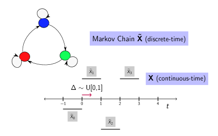
We now apply a random shift Ξ”βˆΌU​[0,1]similar-toΞ”π‘ˆ01\Delta\sim U[0,1] to the {Xt}subscript𝑋𝑑\{X_{t}\} process to transform the non-stationary continuous time process into a stationary one. Let us denote this stationary process by 𝐗𝐗\mathbf{X}. The process 𝐗𝐗\mathbf{X} is observed through the Gaussian channel in (1) at snr=1snr1{\text{snr}}=1, with 𝐘𝐘\mathbf{Y} denoting the channel output process. This procedure is illustrated in Fig. 7
Refer to caption
Figure 7: Construction of the stationary continuous-time process 𝐗𝐗\mathbf{X} from the underlying discrete-time Markov Chain 𝐗~~𝐗{\mathbf{\tilde{X}}}.

VII-A1 Time Reversed Process

Consider the discrete-time process 𝐗~(R)superscript~𝐗𝑅\mathbf{\tilde{X}}^{(R)}, denoting the time reversed version of the stationary process 𝐗~~𝐗\mathbf{\tilde{X}}. The reversed process will, in general, not have the same law as the forward process (though it will of course inherit its stationarity from that of 𝐗~~𝐗{\mathbf{\tilde{X}}}). Let us construct an equivalent continuous time process corresponding to 𝐗~(R)superscript~𝐗𝑅\mathbf{\tilde{X}}^{(R)}, using the procedure described above for the process 𝐗~~𝐗\mathbf{\tilde{X}}, and label the resulting stationary continuous-time process by 𝐗(R)superscript𝐗𝑅\mathbf{X}^{(R)}. In the following example, we compare the minimum mean square errors with finite lookahead for the processes 𝐗𝐗\mathbf{X} and 𝐗(R)superscript𝐗𝑅\mathbf{X}^{(R)}, for a certain underlying discrete-time Markov process.

VII-B Proof of Theorem 11, Examples and Discussions

Define a stationary discrete time Markov chain 𝐗~~𝐗\mathbf{\tilde{X}}, on a finite alphabet 𝒳𝒳{\cal X}, characterized by the transition probability matrix 𝒫𝒫{\cal P}.

The intuition behind the choice of alphabet and transition probabilities, is that we would like the Discrete Time Markov Chain (DTMC) to be highly predictable (under mean square error criterion) in the forward direction compared to the time reversed version of the chain. Note that the time reversed Markov chain will have the same stationary distribution, but different transition probabilities. We transform this discrete time Markov chain to a stationary continuous time process by the transformation described above. Because of the difference in the state predictability of the forward and reverse time processes in the DTMC, the continuous time process thus created will have predictability that behaves differently for the forward and the time reversed processes and, in turn, the MSE with finite lookahead will also be depend on whether the process or its time-reversed version is considered.

VII-B1 Infinite SNR scenario

We now concentrate on the case when the signal-to-noise ratio of the channel is infinite. The input to the Gaussian channel is the continuous time process 𝐗𝐗\mathbf{X}, which is constructed based on 𝐗~~𝐗\mathbf{\tilde{X}} as described above. Let us consider negative lookahead d=βˆ’1𝑑1d=-1. For infinite SNR, the filter will know what the underlying process is exactly, so that

lmmse​(βˆ’1,∞)lmmse1\displaystyle{\text{lmmse}}(-1,\infty) =\displaystyle= Var​(X0|Yβˆ’βˆžβˆ’1)Varconditionalsubscript𝑋0superscriptsubscriptπ‘Œ1\displaystyle{\text{Var}}(X_{0}|Y_{-\infty}^{-1}) (100)
=\displaystyle= Var​(X0|Xβˆ’βˆžβˆ’1)Varconditionalsubscript𝑋0superscriptsubscript𝑋1\displaystyle{\text{Var}}(X_{0}|X_{-\infty}^{-1}) (101)
=\displaystyle= Var​(X~0|X~βˆ’1),Varconditionalsubscript~𝑋0subscript~𝑋1\displaystyle{\text{Var}}(\tilde{X}_{0}|\tilde{X}_{-1}), (102)

where (102) follows from the Markovity of 𝐗~~𝐗\mathbf{\tilde{X}}. Note that the quantity in (102) is the prediction variance of the DTMC 𝐗~~𝐗\mathbf{\tilde{X}}. Let Ξ½:𝒳→ℝ:πœˆβ†’π’³β„\nu:{\cal X}\to\mathbb{R} be any probability measure on the finite alphabet 𝒳𝒳{\cal X} and V​[Ξ½]𝑉delimited-[]𝜈V[\nu] be the variance of this distribution. Let ΞΌ,P​(X~i+1|X~i)πœ‡π‘ƒconditionalsubscript~𝑋𝑖1subscript~𝑋𝑖\mu,P(\tilde{X}_{i+1}|\tilde{X}_{i}) denote respectively, the stationary distribution and the probability transition matrix of the Markov chain 𝐗~~𝐗\mathbf{\tilde{X}}. Then the prediction variance is given by

Var(X~0|X~βˆ’1)=βˆ‘xβˆˆπ’³ΞΌ(x)V[P(β‹…|x)].\displaystyle{\text{Var}}(\tilde{X}_{0}|\tilde{X}_{-1})=\sum_{x\in{\cal X}}\mu(x)V[P(\cdot|x)]. (103)

In the infinite SNR setting, it is straightforward to see that

lmmse​(d,∞)=0,βˆ€dβ‰₯0.formulae-sequencelmmse𝑑0for-all𝑑0\displaystyle{\text{lmmse}}(d,\infty)=0,\hskip 20.00003pt\forall d\geq 0. (104)

Since the process 𝐗𝐗\mathbf{X} is constructed by a uniformly random shift according to a U​[0,1]π‘ˆ01U[0,1] law, for each βˆ’1≀d≀01𝑑0-1\leq d\leq 0, we have

lmmse​(d,∞)=|d|​Var​(X~0|X~βˆ’1),βˆ’1≀d≀0.formulae-sequencelmmse𝑑𝑑Varconditionalsubscript~𝑋0subscript~𝑋11𝑑0\displaystyle{\text{lmmse}}(d,\infty)=|d|{\text{Var}}(\tilde{X}_{0}|\tilde{X}_{-1}),\hskip 10.00002pt-1\leq d\leq 0. (105)

For fixed d∈[βˆ’1,0]𝑑10d\in[-1,0], with probability 1βˆ’|d|1𝑑1-|d|, the process Y∞dsuperscriptsubscriptπ‘Œπ‘‘Y_{\infty}^{d} will sample X~0subscript~𝑋0\tilde{X}_{0} in which case the resulting mean squared error is 00 at infinite SNR. Alternately, with probability |d|𝑑|d| the error will be given by the prediction variance, i.e Var​(X~0|X~βˆ’1)Varconditionalsubscript~𝑋0subscript~𝑋1{\text{Var}}(\tilde{X}_{0}|\tilde{X}_{-1}), which gives rise to (105). A similar analysis can be performed for the time-reversed DTMC 𝐗~(R)superscript~𝐗𝑅\mathbf{\tilde{X}}^{(R)}. Having found analytic expressions for the mmse with lookahead for the infinite SNR case, we show a characteristic plot of the same in Fig. 8. Note the difference in the curves for negative lookahead arises simply due to a difference in prediction variance for the forward and time-reversed DTMC’s 𝐗~~𝐗\mathbf{\tilde{X}} and 𝐗~(R)superscript~𝐗𝑅\mathbf{\tilde{X}}^{(R)}. Since the mmse with lookahead are different for d<0𝑑0d<0 at infinite SNR, they would also be different at a large enough, finite signal-to-noise ratio. This completes the proof of Theorem 11 as stated for d<0𝑑0d<0.

To further argue the existence of processes where lmmse​(d,snr)lmmse𝑑snr{\text{lmmse}}(d,{\text{snr}}) are different, also for positive d𝑑d, we provide the following explicit construction of the underlying processes. We then provide plots of the mmse with lookahead for this process, based on Markov Chain Monte Carlo simulations. The associated plots make it clear that lmmse​(d,β‹…)lmmse𝑑⋅{\text{lmmse}}(d,\cdot) are distinct for both processes when d𝑑d is finite and non-zero.

VII-B2 Simulations

Let 𝐗~~𝐗\mathbf{\tilde{X}} be a Discrete Time Markov Chain with the following specifications: The alphabet is 𝒳={5,0,βˆ’5}𝒳505{\cal X}=\{5,0,-5\}. The probability transition matrix 𝒫𝒫{\cal P} is given by:

𝒫=[0.60.4000.20.80.87500.125]𝒫matrix0.60.4000.20.80.87500.125{\cal P}=\begin{bmatrix}0.6&0.4&0\\[3.00003pt] 0&0.2&0.8\\[3.00003pt] 0.875&0&0.125\end{bmatrix}

where 𝒫i​j=P​(X~k+1=xj|X~k=xi)subscript𝒫𝑖𝑗𝑃subscript~π‘‹π‘˜1conditionalsubscriptπ‘₯𝑗subscript~π‘‹π‘˜subscriptπ‘₯𝑖{\cal P}_{ij}=P(\tilde{X}_{k+1}=x_{j}|\tilde{X}_{k}=x_{i}). Note that x1=5,x2=0,x3=βˆ’5formulae-sequencesubscriptπ‘₯15formulae-sequencesubscriptπ‘₯20subscriptπ‘₯35x_{1}=5,x_{2}=0,x_{3}=-5, in the above example. For this markov chain, we can compute the prediction variance according to (103) to obtain Var​(X0|Xβˆ’1)=6.6423Varconditionalsubscript𝑋0subscript𝑋16.6423{\text{Var}}(X_{0}|X_{-1})=6.6423. The stationary prior for this DTMC is ΞΌ=(0.5109,0.2555,0.2336)πœ‡0.51090.25550.2336\mu=(0.5109,0.2555,0.2336). For the reversed process 𝐗~(R)superscript~𝐗𝑅\mathbf{\tilde{X}}^{(R)}, the probability transition matrix is given by

𝒫(R)=[0.600.40.80.2000.8750.125]superscript𝒫𝑅matrix0.600.40.80.2000.8750.125{\cal P}^{(R)}=\begin{bmatrix}0.6&0&0.4\\[3.00003pt] 0.8&0.2&0\\[3.00003pt] 0&0.875&0.125\end{bmatrix}

and the prediction variance is 13.923413.923413.9234.
We performed monte carlo simulations to obtain the MSE with finite lookahead (and lookback) for the forward and time reversed continuous-time processes thus formed. A brief description of the simulation is provided in Appendix D.

VII-B3 Discussion
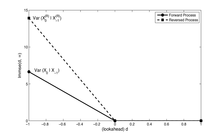
Refer to caption
Figure 8: Minimum mean squared error with negative lookahead for SNR = ∞\infty for the processes 𝐗𝐗\mathbf{X} and 𝐗(𝐑)superscript𝐗𝐑\mathbf{X^{(R)}}.

In Fig. 9, we present the MSE with finite lookahead and lookback for the continuous time process 𝐗𝐗\mathbf{X} and 𝐗(R)superscript𝐗𝑅\mathbf{X}^{(R)} denoting the forward and time-reversed stationary noise-free processes, respectively. From Duncan’s result, we know that the causal and the anti-causal errors must coincide. This is observed (and highlighted in Fig. 10) by the same values for the MSE with 0 lookahead for the forward and reversed processes. Indeed, for both positive and negative lookahead, the MSE’s are different.
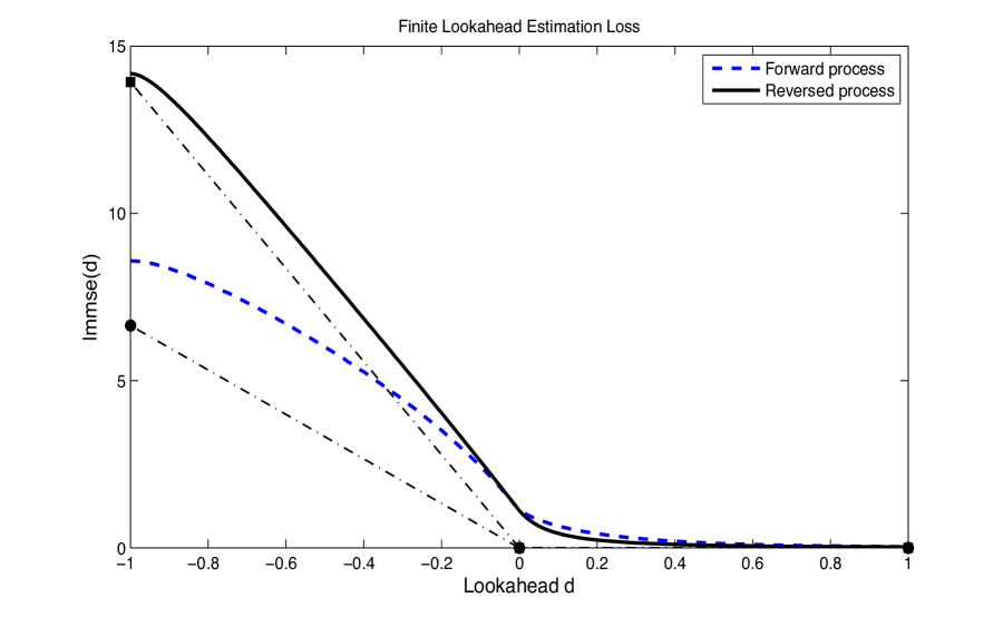
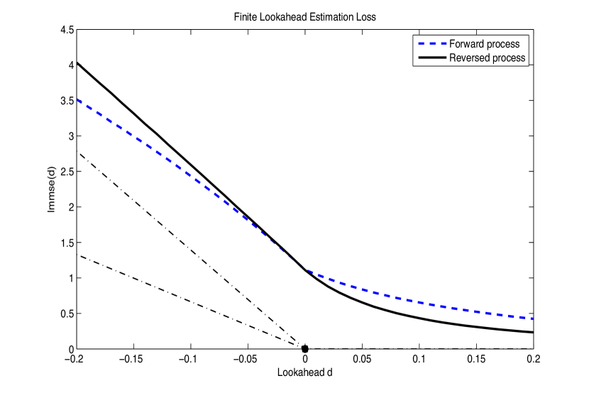
Refer to caption
Figure 9: Comparison of the Estimation Loss with finite lookahead for the Forward and Reverse processes, 𝐗𝐗\mathbf{X} and 𝐗(𝐑)superscript𝐗𝐑\mathbf{X^{(R)}} respectively at SNR=1. For reference, the infinite SNR curves (dashed) are also shown.
Refer to caption
Figure 10: Zoomed in version of Fig. 9. Note that curves coincide at d=0𝑑0d=0, consistent with Duncan’s result (97).

Note that we know the asymptotic behavior of the MSE’s with lookahead. As dβ†’βˆ’βˆžβ†’π‘‘d\to-\infty, the forward(and reverse) MSE will converge to the variance Var​(X~0)Varsubscript~𝑋0{\text{Var}}(\tilde{X}_{0}) of the corresponding underlying DTMC (similarly for the time-reversed chain). For dβ†’βˆžβ†’π‘‘d\to\infty, the MSE’s converge to the non-causal errors respectively (which are naturally equal for the forward and reversed processes). Note that the forward and reversed processes have the same mutual information rate function, as well as the same spectrum. This indicates, that such measures are not capable of characterizing the MMSE with finite lookahead.

The above construction illustrates the complicated nature of lookahead in its role as a link between estimation and information for the Gaussian channel. While answering several important questions, it also raises new ones - Do there exist other informational measures of the input-output laws that are sufficient to characterize the estimation error with lookahead ? Such directions remain for future exploration.

VIII Conclusions

This work can be viewed as a step towards understanding the role of lookahead in information and estimation. We investigate the benefit of finite lookahead in mean squared estimation under additive white Gaussian noise. We study the class of Ornstein-Uhlenbeck processes and explicitly characterize the dependence of squared estimation loss on lookahead and SNR. We extend this result to the class of processes that can be expressed as mixtures of Ornstein-Uhlenbeck processes, and use this characterization to present bounds on the finite lookahead MMSE for a class of Gaussian processes. We observe that Gaussian input processes with rational spectra have the finite lookahead MMSE converging exponentially rapidly from the causal, to the non-causal MMSE. We define and obtain relationships for the information utility of lookahead. We then present an expectation identity for a generalized observation model, which presents the filtering error as a double integral, over lookahead and SNR - of the estimation error with finite lookahead. Finally, we illustrate through means of an example that the mutual information rate function does not uniquely characterize the behavior of estimation error with lookahead, except in the special cases of 00 and infinite lookahead. Our example shows that the finite lookahead MMSE depends on features of the process that are not captured by the information rate function, or indeed, the entire spectrum.

Appendix A

In this appendix we prove Lemma 1. Employing the continuous-time Kalman-Bucy filtering framework (cf. [14] for a detailed presentation), we obtain the following differential equation for the error covariance etsubscript𝑒𝑑e_{t} = Var(Xt|Y0tconditionalsubscript𝑋𝑑superscriptsubscriptπ‘Œ0𝑑X_{t}|Y_{0}^{t})

d​etd​t𝑑subscript𝑒𝑑𝑑𝑑\displaystyle\frac{de_{t}}{dt} =\displaystyle= βˆ’2​α​etβˆ’Ξ³β€‹et2+Ξ²2,2𝛼subscript𝑒𝑑𝛾subscriptsuperscript𝑒2𝑑superscript𝛽2\displaystyle-2\alpha e_{t}-\gamma e^{2}_{t}+\beta^{2}, (106)

where e0=RX​(0)=Ξ²22​αsubscript𝑒0subscript𝑅𝑋0superscript𝛽22𝛼e_{0}=R_{X}(0)=\frac{\beta^{2}}{2\alpha}. We integrate over limits 00 to d𝑑d and re-arrange terms to get the desired result,

∫0dd​etβˆ’2​α​etβˆ’Ξ³β€‹et2+Ξ²2superscriptsubscript0𝑑𝑑subscript𝑒𝑑2𝛼subscript𝑒𝑑𝛾subscriptsuperscript𝑒2𝑑superscript𝛽2\displaystyle\int_{0}^{d}\frac{\,de_{t}}{-2\alpha e_{t}-\gamma e^{2}_{t}+\beta^{2}} =\displaystyle= ∫0d𝑑tsuperscriptsubscript0𝑑differential-d𝑑\displaystyle\int_{0}^{d}\,dt (107)
d𝑑\displaystyle d =\displaystyle= 12​α2+γ​β2​log⁑|βˆ’Ξ³β€‹edβˆ’Ξ±βˆ’Ξ±2+γ​β2βˆ’Ξ³β€‹edβˆ’Ξ±+Ξ±2+γ​β2|βˆ’12​α2+γ​β2​log⁑|ρ|,12superscript𝛼2𝛾superscript𝛽2𝛾subscript𝑒𝑑𝛼superscript𝛼2𝛾superscript𝛽2𝛾subscript𝑒𝑑𝛼superscript𝛼2𝛾superscript𝛽212superscript𝛼2𝛾superscript𝛽2𝜌\displaystyle\frac{1}{2\sqrt{\alpha^{2}+\gamma{\beta^{2}}}}\log{\left|\frac{-\gamma{e_{d}}-\alpha-\sqrt{\alpha^{2}+\gamma{\beta^{2}}}}{-\gamma{e_{d}}-\alpha+\sqrt{\alpha^{2}+\gamma{\beta^{2}}}}\right|}-\frac{1}{2\sqrt{\alpha^{2}+\gamma{\beta^{2}}}}\log|\rho|, (108)

which upon simplification yields the following expression for edsubscript𝑒𝑑e_{d}

edsubscript𝑒𝑑\displaystyle e_{d} =\displaystyle= βˆ’Ξ±Ξ³+Ξ±2+γ​β2γ​(e2​d​α2+γ​β2​ρ+1e2​d​α2+γ​β2β€‹Οβˆ’1),𝛼𝛾superscript𝛼2𝛾superscript𝛽2𝛾superscript𝑒2𝑑superscript𝛼2𝛾superscript𝛽2𝜌1superscript𝑒2𝑑superscript𝛼2𝛾superscript𝛽2𝜌1\displaystyle-\frac{\alpha}{\gamma}+\frac{\sqrt{\alpha^{2}+\gamma{\beta^{2}}}}{\gamma}\bigg{(}\frac{e^{2d\sqrt{\alpha^{2}+\gamma{\beta^{2}}}}\rho+1}{e^{2d\sqrt{\alpha^{2}+\gamma{\beta^{2}}}}\rho-1}\bigg{)}, (109)

where ρ𝜌\rho is as defined as

ρ=|γ​RX​(0)+Ξ±2+γ​β2+αγ​RX​(0)βˆ’Ξ±2+γ​β2+Ξ±|.πœŒπ›Ύsubscript𝑅𝑋0superscript𝛼2𝛾superscript𝛽2𝛼𝛾subscript𝑅𝑋0superscript𝛼2𝛾superscript𝛽2𝛼\displaystyle\rho=\left|\frac{\gamma R_{X}(0)+{\sqrt{\alpha^{2}+\gamma{\beta^{2}}}+\alpha}}{\gamma R_{X}(0)-\sqrt{\alpha^{2}+\gamma{\beta^{2}}}+\alpha}\right|. (110)

Appendix B

In this appendix, we illustrate the computation of the MMSE with finite lookahead for a Gaussian process, whose spectrum is an equal mixture of the spectra of two Ornstein-Ulhenbeck processes, parametrized by Ξ±isubscript𝛼𝑖\alpha_{i}, i=1,2𝑖12i=1,2. In this computation, we use the equations developed in Section IV-A.

For simplicity, we will operate in the β€˜s’ domain for the spectra, where the region of convergence of the Laplace transform will be implicit. Recall from (14), that the spectrum of an Ornstein-Ulhenbeck process with parameter α𝛼\alpha is given by

Sα​(s)=1Ξ±2βˆ’s2subscript𝑆𝛼𝑠1superscript𝛼2superscript𝑠2\displaystyle S_{\alpha}(s)=\frac{1}{\alpha^{2}-s^{2}} (111)

Thus, the spectrum of the input process Xtsubscript𝑋𝑑X_{t}, which is a mixture of two Ornstein-Ulhenbeck processes is given by

SX​(s)=12β‹…1Ξ±12βˆ’s2+12β‹…1Ξ±22βˆ’s2subscript𝑆𝑋𝑠⋅121superscriptsubscript𝛼12superscript𝑠2β‹…121superscriptsubscript𝛼22superscript𝑠2\displaystyle S_{X}(s)=\frac{1}{2}\cdot\frac{1}{\alpha_{1}^{2}-s^{2}}+\frac{1}{2}\cdot\frac{1}{\alpha_{2}^{2}-s^{2}} (112)

Under the observation model in (1) at a fixed signal-to-noise ratio snr>0snr0{\text{snr}}>0, the output spectrum is given by:

SY​(s)=1+snr2β‹…[1Ξ±12βˆ’s2+1Ξ±22βˆ’s2]subscriptπ‘†π‘Œπ‘ 1β‹…snr2delimited-[]1superscriptsubscript𝛼12superscript𝑠21superscriptsubscript𝛼22superscript𝑠2\displaystyle S_{Y}(s)=1+\frac{{\text{snr}}}{2}\cdot\big{[}\frac{1}{\alpha_{1}^{2}-s^{2}}+\frac{1}{\alpha_{2}^{2}-s^{2}}\big{]} (113)

Performing the Wiener-Hopf decomposition of the output spectrum in (113), we obtain the following spectral factors:

SY+​(s)=(s+p1)​(s+p2)(Ξ±1+s)​(Ξ±2+s),subscriptsuperscriptπ‘†π‘Œπ‘ π‘ subscript𝑝1𝑠subscript𝑝2subscript𝛼1𝑠subscript𝛼2𝑠\displaystyle S^{+}_{Y}(s)=\frac{(s+p_{1})(s+p_{2})}{(\alpha_{1}+s)(\alpha_{2}+s)}, (114)

and

SYβˆ’β€‹(s)=(sβˆ’p1)​(sβˆ’p2)(Ξ±1βˆ’s)​(Ξ±2βˆ’s),subscriptsuperscriptπ‘†π‘Œπ‘ π‘ subscript𝑝1𝑠subscript𝑝2subscript𝛼1𝑠subscript𝛼2𝑠\displaystyle S^{-}_{Y}(s)=\frac{(s-p_{1})(s-p_{2})}{(\alpha_{1}-s)(\alpha_{2}-s)}, (115)

where p1,p2>0subscript𝑝1subscript𝑝20p_{1},p_{2}>0 are such that pi2superscriptsubscript𝑝𝑖2p_{i}^{2}, i=1,2𝑖12i=1,2 are solutions of k​(x)=0π‘˜π‘₯0k(x)=0, where

k​(x)=x2βˆ’(Ξ±12+Ξ±22+snr)​x+snr2​(Ξ±12+Ξ±22)+Ξ±12​α22.π‘˜π‘₯superscriptπ‘₯2superscriptsubscript𝛼12superscriptsubscript𝛼22snrπ‘₯snr2superscriptsubscript𝛼12superscriptsubscript𝛼22superscriptsubscript𝛼12superscriptsubscript𝛼22\displaystyle k(x)=x^{2}-(\alpha_{1}^{2}+\alpha_{2}^{2}+{\text{snr}})x+\frac{{\text{snr}}}{2}(\alpha_{1}^{2}+\alpha_{2}^{2})+\alpha_{1}^{2}\alpha_{2}^{2}. (116)

Note that SYβˆ’β€‹(s)=SY+​(βˆ’s)subscriptsuperscriptπ‘†π‘Œπ‘ subscriptsuperscriptπ‘†π‘Œπ‘ S^{-}_{Y}(s)=S^{+}_{Y}(-s). Invoking (54), the transfer function of the optimal non-causal filter H​(β‹…)𝐻⋅H(\cdot) is characterized by

H​(s)𝐻𝑠\displaystyle H(s) =snr​SX​(s)SYβˆ’β€‹(s)absentsnrsubscript𝑆𝑋𝑠subscriptsuperscriptπ‘†π‘Œπ‘ \displaystyle=\frac{\sqrt{{\text{snr}}}S_{X}(s)}{S^{-}_{Y}(s)} (117)
=s​n​r2​(Ξ±12+Ξ±22)βˆ’s​n​r​s2(sβˆ’p1)​(sβˆ’p2)​(Ξ±1+s)​(Ξ±2+s)absentπ‘ π‘›π‘Ÿ2superscriptsubscript𝛼12superscriptsubscript𝛼22π‘ π‘›π‘Ÿsuperscript𝑠2𝑠subscript𝑝1𝑠subscript𝑝2subscript𝛼1𝑠subscript𝛼2𝑠\displaystyle=\frac{\frac{\sqrt{snr}}{2}(\alpha_{1}^{2}+\alpha_{2}^{2})-\sqrt{snr}s^{2}}{(s-p_{1})(s-p_{2})(\alpha_{1}+s)(\alpha_{2}+s)} (118)
=u1sβˆ’p1+u2sβˆ’p2+v1Ξ±1+s+v2Ξ±2+s,absentsubscript𝑒1𝑠subscript𝑝1subscript𝑒2𝑠subscript𝑝2subscript𝑣1subscript𝛼1𝑠subscript𝑣2subscript𝛼2𝑠\displaystyle=\frac{u_{1}}{s-p_{1}}+\frac{u_{2}}{s-p_{2}}+\frac{v_{1}}{\alpha_{1}+s}+\frac{v_{2}}{\alpha_{2}+s}, (119)

where (118) follows from (112) and (115); and (119) denotes the partial fraction decomposition of the expression in (118). Having derived an exact expression for the Wiener filter, we are now in a position to compute the desired quantity, i.e. lmmse​(d,snr)lmmse𝑑snr{\text{lmmse}}(d,{\text{snr}}). From (60) we have,

lmmse​(d,snr)=mmse​(snr)+βˆ«βˆ’βˆžβˆ’dh2​(t)​𝑑t.lmmse𝑑snrmmsesnrsuperscriptsubscript𝑑superscriptβ„Ž2𝑑differential-d𝑑\displaystyle{\text{lmmse}}(d,{\text{snr}})={\text{mmse}}({\text{snr}})+\int_{-\infty}^{-d}h^{2}(t)\,dt. (120)

From the classical result by Wiener [13], we know that the mmse of a Gaussian process is given by

mmse​(snr)=βˆ«βˆ’βˆžβˆžSX​(j​ω)1+snr​SX​(j​ω)​d​ω2​π.mmsesnrsuperscriptsubscriptsubscriptπ‘†π‘‹π‘—πœ”1snrsubscriptπ‘†π‘‹π‘—πœ”π‘‘πœ”2πœ‹\displaystyle{\text{mmse}}({\text{snr}})=\int_{-\infty}^{\infty}\frac{S_{X}(j\omega)}{1+{\text{snr}}\,S_{X}(j\omega)}\,\frac{d\omega}{2\pi}. (121)

Using (119) and (120), we are now in a position to explicitly compute the mmse with finite lookahead for the X𝑋X process corrupted by the Gaussian channel:

lmmseX​(d,snr)={mmse​(snr)+u122​p1​eβˆ’2​p1​d+u222​p2​eβˆ’2​p2​d+u1​u2p1+p2​eβˆ’(p1+p2)​dif ​dβ‰₯0mmse​(snr)+C+v122​α1​e2​α1​d+v222​α2​e2​α2​d+v1​v2Ξ±1+Ξ±2​e(Ξ±1+Ξ±2)​dif ​d<0,subscriptlmmse𝑋𝑑snrcasesmmsesnrsuperscriptsubscript𝑒122subscript𝑝1superscript𝑒2subscript𝑝1𝑑superscriptsubscript𝑒222subscript𝑝2superscript𝑒2subscript𝑝2𝑑subscript𝑒1subscript𝑒2subscript𝑝1subscript𝑝2superscript𝑒subscript𝑝1subscript𝑝2𝑑if 𝑑0mmsesnr𝐢superscriptsubscript𝑣122subscript𝛼1superscript𝑒2subscript𝛼1𝑑superscriptsubscript𝑣222subscript𝛼2superscript𝑒2subscript𝛼2𝑑subscript𝑣1subscript𝑣2subscript𝛼1subscript𝛼2superscript𝑒subscript𝛼1subscript𝛼2𝑑if 𝑑0\displaystyle{\text{lmmse}}_{X}(d,{\text{snr}})=\left\{\begin{array}[]{ll}{\text{mmse}}({\text{snr}})+\frac{u_{1}^{2}}{2p_{1}}e^{-2p_{1}\,d}+\frac{u_{2}^{2}}{2p_{2}}e^{-2p_{2}\,d}+\frac{u_{1}u_{2}}{p_{1}+p_{2}}e^{-(p_{1}+p_{2})\,d}&\mbox{if }d\geq 0\\ {\text{mmse}}({\text{snr}})+C+\frac{v_{1}^{2}}{2\alpha_{1}}e^{2\alpha_{1}\,d}+\frac{v_{2}^{2}}{2\alpha_{2}}e^{2\alpha_{2}\,d}+\frac{v_{1}v_{2}}{\alpha_{1}+\alpha_{2}}e^{(\alpha_{1}+\alpha_{2})\,d}&\mbox{if }d<0\end{array}\right., (124)

where

C=u122​p1+u222​p2+u1​u2p1+p2βˆ’v122​α1βˆ’v222​α2βˆ’v1​v2Ξ±1+Ξ±2.𝐢superscriptsubscript𝑒122subscript𝑝1superscriptsubscript𝑒222subscript𝑝2subscript𝑒1subscript𝑒2subscript𝑝1subscript𝑝2superscriptsubscript𝑣122subscript𝛼1superscriptsubscript𝑣222subscript𝛼2subscript𝑣1subscript𝑣2subscript𝛼1subscript𝛼2\displaystyle C=\frac{u_{1}^{2}}{2p_{1}}+\frac{u_{2}^{2}}{2p_{2}}+\frac{u_{1}u_{2}}{p_{1}+p_{2}}-\frac{v_{1}^{2}}{2\alpha_{1}}-\frac{v_{2}^{2}}{2\alpha_{2}}-\frac{v_{1}v_{2}}{\alpha_{1}+\alpha_{2}}. (125)

Recall the rate of convergence of the mmse with lookahead, from causal to non-causal error, was defined as

pd≐lmmse​(d,snr)βˆ’mmse​(snr)cmmse​(snr)βˆ’mmse​(snr).approaches-limitsubscript𝑝𝑑lmmse𝑑snrmmsesnrcmmsesnrmmsesnr\displaystyle p_{d}\doteq\frac{{\text{lmmse}}(d,{\text{snr}})-{\text{mmse}}({\text{snr}})}{{\text{cmmse}}({\text{snr}})-{\text{mmse}}({\text{snr}})}. (126)

For the Gaussian input process with spectrum as given in (112), we can use (124) to compute the quantity pdsubscript𝑝𝑑p_{d}:

pd=1C​[u122​p1​eβˆ’2​p1​d+u222​p2​eβˆ’2​p2​d+u1​u2p1+p2​eβˆ’(p1+p2)​d]subscript𝑝𝑑1𝐢delimited-[]superscriptsubscript𝑒122subscript𝑝1superscript𝑒2subscript𝑝1𝑑superscriptsubscript𝑒222subscript𝑝2superscript𝑒2subscript𝑝2𝑑subscript𝑒1subscript𝑒2subscript𝑝1subscript𝑝2superscript𝑒subscript𝑝1subscript𝑝2𝑑\displaystyle p_{d}=\frac{1}{C}\left[\,\frac{u_{1}^{2}}{2p_{1}}e^{-2p_{1}\,d}+\frac{u_{2}^{2}}{2p_{2}}e^{-2p_{2}\,d}+\frac{u_{1}u_{2}}{p_{1}+p_{2}}e^{-(p_{1}+p_{2})\,d}\right] (127)

Clearly pdβ†’0β†’subscript𝑝𝑑0p_{d}{\rightarrow}0 for large d𝑑d, in accordance with Lemma 9.

Appendix C

Let e^t≐Var​(Xt|Y0t,X0)approaches-limitsubscript^𝑒𝑑Varconditionalsubscript𝑋𝑑superscriptsubscriptπ‘Œ0𝑑subscript𝑋0\hat{e}_{t}\doteq{\text{Var}}(X_{t}|Y_{0}^{t},X_{0}), and notice that e^tsubscript^𝑒𝑑\hat{e}_{t} satisfies the Kalman-Bucy differential equation (106), with the initial condition e^0=0subscript^𝑒00\hat{e}_{0}=0. Applying a similar integration procedure to the one described above, we find that

e^dsubscript^𝑒𝑑\displaystyle\hat{e}_{d} =\displaystyle= βˆ’Ξ±Ξ³+Ξ±2+γ​β2γ​(e2​d​α2+γ​β2​ρ^βˆ’1e2​d​α2+γ​β2​ρ^+1),𝛼𝛾superscript𝛼2𝛾superscript𝛽2𝛾superscript𝑒2𝑑superscript𝛼2𝛾superscript𝛽2^𝜌1superscript𝑒2𝑑superscript𝛼2𝛾superscript𝛽2^𝜌1\displaystyle-\frac{\alpha}{\gamma}+\frac{\sqrt{\alpha^{2}+\gamma{\beta^{2}}}}{\gamma}\bigg{(}\frac{e^{2d\sqrt{\alpha^{2}+\gamma{\beta^{2}}}}\hat{\rho}-1}{e^{2d\sqrt{\alpha^{2}+\gamma{\beta^{2}}}}\hat{\rho}+1}\bigg{)}, (128)

with

ρ^=Ξ±2+γ​β2+Ξ±Ξ±2+γ​β2βˆ’Ξ±.^𝜌superscript𝛼2𝛾superscript𝛽2𝛼superscript𝛼2𝛾superscript𝛽2𝛼\displaystyle\hat{\rho}=\frac{\sqrt{\alpha^{2}+\gamma{\beta^{2}}}+\alpha}{\sqrt{\alpha^{2}+\gamma{\beta^{2}}}-\alpha}. (129)

We define the quantity,

τ≐α2+γ​β2.approaches-limit𝜏superscript𝛼2𝛾superscript𝛽2\displaystyle\tau\doteq\sqrt{\alpha^{2}+\gamma{\beta^{2}}}. (130)

Equations (19) and (20) can be rewritten as

cmmse(Ξ³)=Ο„βˆ’Ξ±Ξ³,mmse(Ξ³)=Ο„2βˆ’Ξ±22​τ​γ=cmmse(Ξ³)Ο„+Ξ±2​τ.\displaystyle{\text{cmmse}}(\gamma)=\frac{\tau-\alpha}{\gamma}\quad,\quad{\text{mmse}}(\gamma)=\frac{\tau^{2}-\alpha^{2}}{2\tau\gamma}={\text{cmmse}}(\gamma)\frac{\tau+\alpha}{2\tau}. (131)

Using the above relations, we have

Var​(Xd|Y0d,X0)Varconditionalsubscript𝑋𝑑superscriptsubscriptπ‘Œ0𝑑subscript𝑋0\displaystyle{\text{Var}}(X_{d}|Y_{0}^{d},X_{0}) =\displaystyle= βˆ’Ξ±Ξ³+τγ​(e2​d​τ​(Ο„+Ξ±)βˆ’(Ο„βˆ’Ξ±)e2​d​τ​(Ο„+Ξ±)+(Ο„βˆ’Ξ±))π›Όπ›Ύπœπ›Ύsuperscript𝑒2π‘‘πœπœπ›Όπœπ›Όsuperscript𝑒2π‘‘πœπœπ›Όπœπ›Ό\displaystyle-\frac{\alpha}{\gamma}+\frac{\tau}{\gamma}\left(\frac{e^{2d\tau}(\tau+\alpha)-(\tau-\alpha)}{e^{2d\tau}(\tau+\alpha)+(\tau-\alpha)}\right) (132)
=\displaystyle= cmmse​(Ξ³)βˆ’2​τγ​(Ο„βˆ’Ξ±e2​d​τ​(Ο„+Ξ±)+(Ο„βˆ’Ξ±)).cmmse𝛾2πœπ›Ύπœπ›Όsuperscript𝑒2π‘‘πœπœπ›Όπœπ›Ό\displaystyle{\text{cmmse}}(\gamma)-\frac{2\tau}{\gamma}\left(\frac{\tau-\alpha}{e^{2d\tau}(\tau+\alpha)+(\tau-\alpha)}\right). (133)

Integrating, we obtain

∫0tVar​(Xs|Y0s,X0)​𝑑s=t​cmmse​(Ξ³)βˆ’2​τγ​[tβˆ’12​τ​log⁑(e2​τ​t​(Ο„+Ξ±)+(Ο„βˆ’Ξ±)2​τ)].superscriptsubscript0𝑑Varconditionalsubscript𝑋𝑠superscriptsubscriptπ‘Œ0𝑠subscript𝑋0differential-d𝑠𝑑cmmse𝛾2πœπ›Ύdelimited-[]𝑑12𝜏superscript𝑒2πœπ‘‘πœπ›Όπœπ›Ό2𝜏\displaystyle\int_{0}^{t}{\text{Var}}(X_{s}|Y_{0}^{s},X_{0})ds=t{\text{cmmse}}(\gamma)-\frac{2\tau}{\gamma}\left[t-\frac{1}{2\tau}\log{\left(\frac{e^{2{\tau}t}(\tau+\alpha)+(\tau-\alpha)}{2\tau}\right)}\right]. (134)

Since the Ornstein-Uhlenbeck process is Markov, it satisfies Var​(Xt|Yβˆ’βˆžt,X0)=Var​(Xt|Y0t,X0)Varconditionalsubscript𝑋𝑑superscriptsubscriptπ‘Œπ‘‘subscript𝑋0Varconditionalsubscript𝑋𝑑superscriptsubscriptπ‘Œ0𝑑subscript𝑋0{\text{Var}}(X_{t}|Y_{-\infty}^{t},X_{0})={\text{Var}}(X_{t}|Y_{0}^{t},X_{0}) for any tβ‰₯0𝑑0t\geq 0. We may therefore use the relation in (74) in conjunction with (134) to write an expression for the information utility of lookahead for this process:

2​U​(t)2π‘ˆπ‘‘\displaystyle 2U(t) =\displaystyle= 2​τ​tβˆ’log⁑(e2​τ​t​(Ο„+Ξ±)+(Ο„βˆ’Ξ±)2​τ)2πœπ‘‘superscript𝑒2πœπ‘‘πœπ›Όπœπ›Ό2𝜏\displaystyle 2{\tau}t-\log{\left(\frac{e^{2{\tau}t}(\tau+\alpha)+(\tau-\alpha)}{2\tau}\right)} (135)
=\displaystyle= βˆ’log⁑(eβˆ’2​τ​t+(1βˆ’eβˆ’2​τ​t)​τ+Ξ±2​τ).superscript𝑒2πœπ‘‘1superscript𝑒2πœπ‘‘πœπ›Ό2𝜏\displaystyle-\log{\left(e^{-2{\tau}t}+(1-e^{-2{\tau}t})\frac{\tau+\alpha}{2\tau}\right)}. (136)

Since the Ornstein-Uhlenbeck process is also stationary and Gaussian, we may plug our expression for U​(β‹…)π‘ˆβ‹…U(\cdot) into (75) and obtain the finite lookahead MMSE,

lmmse​(d,Ξ³)lmmse𝑑𝛾\displaystyle{\text{lmmse}}(d,\gamma) =\displaystyle= cmmse​(Ξ³)β‹…eβˆ’2​U​(d)=cmmse​(Ξ³)​(eβˆ’2​τ​d+(1βˆ’eβˆ’2​τ​d)​τ+Ξ±2​τ)β‹…cmmse𝛾superscript𝑒2π‘ˆπ‘‘cmmse𝛾superscript𝑒2πœπ‘‘1superscript𝑒2πœπ‘‘πœπ›Ό2𝜏\displaystyle{\text{cmmse}}(\gamma){\cdot}e^{-2{U(d)}}={\text{cmmse}}(\gamma)\left(e^{-2{\tau}d}+(1-e^{-2{\tau}d})\frac{\tau+\alpha}{2\tau}\right) (137)
=\displaystyle= eβˆ’2​τ​d​cmmse​(Ξ³)+(1βˆ’eβˆ’2​τ​d)​mmse​(Ξ³),superscript𝑒2πœπ‘‘cmmse𝛾1superscript𝑒2πœπ‘‘mmse𝛾\displaystyle e^{-2{\tau}d}{\text{cmmse}}(\gamma)+(1-e^{-2{\tau}d}){\text{mmse}}(\gamma), (138)

which recovers Lemma 4 for positive lookahead.

Appendix D

Let 𝐗~~𝐗\mathbf{\tilde{X}} be a stationary discrete time Markov chain, with known probability transition matrix 𝒫𝒫{\cal P}. Let Y~i​(Ξ³)subscript~π‘Œπ‘–π›Ύ\tilde{Y}_{i}(\gamma) denote the noisy observation of X~isubscript~𝑋𝑖\tilde{X}_{i} corrupted via independent Gaussian noise with the signal to noise ratio of the measurement being γ𝛾\gamma. I.e.,

Y~i​(Ξ³)=γ​X~i+W~Ξ³(i),subscript~π‘Œπ‘–π›Ύπ›Ύsubscript~𝑋𝑖subscriptsuperscript~π‘Šπ‘–π›Ύ\displaystyle\tilde{Y}_{i}(\gamma)=\gamma\tilde{X}_{i}+\tilde{W}^{(i)}_{\gamma}, (139)

where {W~β‹…(i)}isubscriptsubscriptsuperscript~π‘Šπ‘–β‹…π‘–\{\tilde{W}^{(i)}_{\cdot}\}_{i} are independent standard Brownian motions, which are further independent of the X~isubscript~𝑋𝑖\tilde{X}_{i}’s. Let 𝐗𝐗\mathbf{X} denote the corresponding stationary continuous time process generated by the process described in Section VII-A, and let 𝐘𝐘\mathbf{Y} denote the noisy process generated via the continuous time Gaussian channel (1) with input 𝐗𝐗\mathbf{X}, i.e.

d​Yt=Xt​d​t+d​Wt,𝑑subscriptπ‘Œπ‘‘subscript𝑋𝑑𝑑𝑑𝑑subscriptπ‘Šπ‘‘\displaystyle dY_{t}=X_{t}\,dt+\,dW_{t}, (140)

where Wβ‹…subscriptπ‘Šβ‹…W_{\cdot} is a standard Brownian motion independent of the 𝐗𝐗\mathbf{X} process.
Define

h​(Ξ³1,Ξ³2)=Var​(X~0|Y~βˆ’βˆžβˆ’1​(1),Y~0​(Ξ³1),Y~1​(Ξ³2))β„Žsubscript𝛾1subscript𝛾2Varconditionalsubscript~𝑋0superscriptsubscript~π‘Œ11subscript~π‘Œ0subscript𝛾1subscript~π‘Œ1subscript𝛾2\displaystyle h(\gamma_{1},\gamma_{2})={\text{Var}}(\tilde{X}_{0}|\tilde{Y}_{-\infty}^{-1}(1),\tilde{Y}_{0}(\gamma_{1}),\tilde{Y}_{1}(\gamma_{2})) (141)

Let, as before

lmmse​(d)=Var​(X0|Yβˆ’βˆžd).lmmse𝑑Varconditionalsubscript𝑋0superscriptsubscriptπ‘Œπ‘‘\displaystyle{\text{lmmse}}(d)={\text{Var}}(X_{0}|Y_{-\infty}^{d}). (142)

For 0<d<10𝑑10<d<1, note that

lmmse​(d)=∫0dh​(1,dβˆ’u)​𝑑u+∫d1h​(1+dβˆ’u,0)​𝑑u.lmmse𝑑superscriptsubscript0π‘‘β„Ž1𝑑𝑒differential-d𝑒superscriptsubscript𝑑1β„Ž1𝑑𝑒0differential-d𝑒\displaystyle{\text{lmmse}}(d)=\int_{0}^{d}h(1,d-u)\,du+\int_{d}^{1}h(1+d-u,0)\,du. (143)

D-A MCMC approach to estimating h​(β‹…,β‹…)β„Žβ‹…β‹…h(\cdot,\cdot)

Note that {X~i,Y~i}iβ‰₯1subscriptsubscript~𝑋𝑖subscript~π‘Œπ‘–π‘–1\{\tilde{X}_{i},\tilde{Y}_{i}\}_{i\geq 1} for a Hidden Markov process. By using state estimation for HMP’s, the following computation can be performed for any i𝑖i,

X~^i=𝔼​[X~i|Y~1iβˆ’1​(1),Y~i​(Ξ³1),Y~i+1​(Ξ³2)]subscript^~𝑋𝑖𝔼delimited-[]conditionalsubscript~𝑋𝑖superscriptsubscript~π‘Œ1𝑖11subscript~π‘Œπ‘–subscript𝛾1subscript~π‘Œπ‘–1subscript𝛾2\displaystyle\hat{\tilde{X}}_{i}=\mathbb{E}[\tilde{X}_{i}|\tilde{Y}_{1}^{i-1}(1),\tilde{Y}_{i}(\gamma_{1}),\tilde{Y}_{i+1}(\gamma_{2})] (144)

Also, one can observe that

1Mβ€‹βˆ‘i=1M(X~iβˆ’X~^i)2β†’h​(Ξ³1,Ξ³2),β†’1𝑀superscriptsubscript𝑖1𝑀superscriptsubscript~𝑋𝑖subscript^~𝑋𝑖2β„Žsubscript𝛾1subscript𝛾2\displaystyle\frac{1}{M}\sum_{i=1}^{M}(\tilde{X}_{i}-\hat{\tilde{X}}_{i})^{2}\to h(\gamma_{1},\gamma_{2}), (145)

as Mβ†’βˆžβ†’π‘€M\to\infty. In the simulations, we chose M=10000𝑀10000M=10000. For this value of M𝑀M, the quantity in the l.h.s. of (145) was used to approximate h​(β‹…,β‹…)β„Žβ‹…β‹…h(\cdot,\cdot), which was then used in the expression for lmmse​(d)lmmse𝑑{\text{lmmse}}(d) in (143) to obtain the desired values of MSE with finite lookahead, via a monte carlo approach.

Based on a similar approach, it is also possible to compute via MCMC, lmmse​(d)lmmse𝑑{\text{lmmse}}(d) for βˆ’1<d<01𝑑0-1<d<0.

Acknowledgment

This work has been partially supported under a Stanford Graduate Fellowship, the National Science Foundation (NSF) under grant agreement CCF-0939370, and the Israel Science Foundation (ISF).

References

  • [1] T. E. Duncan, β€œOn the calculation of Mutual Information”, SIAM J. Appl. Math., vol. 19, pp. 215-220, Jul. 1970.
  • [2] D. Guo, S. Shamai and S. VerdΓΊ, ”Mutual Information and minimum mean-square error in Gaussian channels”, IEEE Trans. Information theory, vol. IT-51, no. 4, pp.1261–1283, Apr. 2005.
  • [3] T. Weissman, β€œThe Relationship Between Causal and Noncausal Mismatched Estimation in Continuous-Time AWGN Channels”, IEEE Trans. Information theory, vol. 56, no. 9, pp. 4256–4273, September 2010.
  • [4] S. VerdΓΊ, β€œMismatched Estimation and relative Entropy”, IEEE Trans. Information theory, vol 56., no. 8, pp. 3712-3720, Aug. 2010.
  • [5] K. Venkat, T. Weissman, β€œPointwise Relations between Information and Estimation in Gaussian Noise”, IEEE Transactions on Information Theory, vol. 58, no. 10, pp. 6264–6281, October 2012.
  • [6] I. Karatzas and A. E. Shreve, Brownian Motion and Stochastic Calculus, 2nd ed. Springer-Verlag, New York, 1988.
  • [7] R. Sh. Liptser, Y. Steinberg, B. Z. Bobrovsky, and Z. Schuss, β€œFixed lag smoothing of scalar diffusions. Part I. The filtering-smoothing equation”, Stochastic Processes and their Applications, 64, issue 2, p. 237–255, (1996).
  • [8] G. E. Uhlenbeck and L. S. Ornstein, β€œOn the theory of Brownian Motion”, Phys.Rev., Vol. 36, No. 5, pp. 823–841, September 1930.
  • [9] J. L. Doob, β€œThe Brownian Movement and Stochastic Equations”, Annals of Mathematics, Second Series, Vol. 43, No. 2, pp. 351–369, April 1942.
  • [10] T. Kailath, A. H. Sayed, B. Hassibi, Linear Estimation, Prentice Hall, 2000.
  • [11] N. Wiener, E. Hopf, β€œUeber eine Klasse singulΓ€rer Integralgleichungen”, Sitzungber. Akad. Wiss. Berlin, pp. 696–706, 1931.
  • [12] M. C. Yovits, J. L. Jackson, β€œLinear Filter optimization with game theory considerations,” Proc. IRE, vol. 43, 1955.
  • [13] N. Wiener, Extrapolation, Ineterpolation, and Smoothing of Stationary Time Series, with Engineering Applications, New York: Wiley 1942.
  • [14] R. S. Lipster, A. N. Shiryaev, Statistics of Random Processes, Vol. I, Springer, 1977.
  • [15] M. Zakai, β€œOn Mutual Information, Likelihood Ratios, and Estimation Error for the Additive Gaussian Channel”, IEEE Transactions on Information theory, vol. 51, No. 9, September 2005.