SISSA 45/2012/EP
Phenomenology of Minimal Unified Tree Level Gauge Mediation at the LHC

Maurizio Monacoa𝑎{}^{\,a}, Maurizio Pierinib𝑏{}^{\,b}, Andrea Romaninoa𝑎{}^{\,a} and Martin Spinratha𝑎{}^{\,a}
asuperscript𝑎\mbox{}^{a}
SISSA/ISAS and INFN, I–34136 Trieste, Italy
bsuperscript𝑏\mbox{}^{b} CERN, CH-1211 Geneva 23, Switzerland
Abstract

We study the collider phenomenology of the minimal unified version of the supersymmetry breaking scheme called Tree-level Gauge Mediation. We identify a peculiar source of gaugino mass non-universality related to the necessary SU(5)𝑆𝑈5SU(5)-breaking in the light fermion mass ratios and a gaugino mass sum rule at the GUT scale, 3M2+2M3=5M13subscript𝑀22subscript𝑀35subscript𝑀13M_{2}+2M_{3}=5M_{1}, which represents a smoking gun of this scenario, together with the known tree-level sfermion mass ratio m~dc,l=2m~q,uc,ecsubscript~𝑚superscript𝑑𝑐𝑙2subscript~𝑚𝑞superscript𝑢𝑐superscript𝑒𝑐\tilde{m}_{d^{c},l}=\sqrt{2}\,\tilde{m}_{q,u^{c},e^{c}}. The boundary conditions of the soft SUSY breaking terms can be parameterised in terms of six relevant parameters only (plus the sign of the μ𝜇\mu-parameter). We analyze the parameter space and define three benchmark points, corresponding to the three possible NLSPs, a bino- or wino-like neutralino or the stau. The LSP is the gravitino as in gauge mediation. For these benchmark points we show possible signatures at the LHC focusing on the Razor variable. We also comment on the Higgs mass.

1 Introduction

The aim of this paper is to spell out the LHC phenomenology of a simple, unified realization of the tree-level gauge mediation (TGM) supersymmetry breaking scheme [1, 2]. In TGM, supersymmetry breaking takes place as usual in a hidden sector and is communicated at the tree level to the MSSM fields by means of superheavy vector fields associated to a broken U(1)𝑈1U(1) gauge group. TGM therefore requires an extension of the Standard Model (SM) gauge group GSMsubscript𝐺SMG_{\text{SM}} to at least GSM×U(1)subscript𝐺SM𝑈1G_{\text{SM}}\times U(1). The (non-anomalous) extra U(1)𝑈1U(1) is spontaneously broken at a high scale M𝑀M. The corresponding vector field V𝑉V acquires a mass MV=gMsubscript𝑀𝑉𝑔𝑀M_{V}=gM, where, g𝑔g is the U(1)𝑈1U(1) gauge coupling. If both the observable superfield f𝑓f and the supersymmetry breaking field Z𝑍Z, Z=Fθ2delimited-⟨⟩𝑍𝐹superscript𝜃2\big{\langle}Z\big{\rangle}=F\theta^{2}, are charged under U(1)𝑈1U(1), V𝑉V plays the role of the supersymmetry breaking messenger, as in Fig. 1. At the scale M𝑀M, the sfermion f~~𝑓\tilde{f} acquires a soft mass given by

m~f2=g2XfXZ|F|2MV2,subscriptsuperscript~𝑚2𝑓superscript𝑔2subscript𝑋𝑓subscript𝑋𝑍superscript𝐹2subscriptsuperscript𝑀2𝑉\tilde{m}^{2}_{f}=\frac{g^{2}X_{f}X_{Z}|F|^{2}}{M^{2}_{V}}\;, (1)

where Xfsubscript𝑋𝑓X_{f} and XZsubscript𝑋𝑍X_{Z} are the charges of f𝑓f and Z𝑍Z under U(1)𝑈1U(1). This simple way to communicate supersymmetry breaking is particularly suited to realize a simple, complete, and viable model of dynamical supersymmetry breaking [3].

Refer to caption
Figure 1: The U(1)𝑈1U(1) massive vector superfield V𝑉V communicates supersymmetry breaking associated to Z=Fθ2delimited-⟨⟩𝑍𝐹superscript𝜃2\big{\langle}Z\big{\rangle}=F\theta^{2} to the observable field f𝑓f at the tree level.

It is tempting to consider U(1)𝑈1U(1) as part of a grand unified group GGSM×U(1)subscript𝐺SM𝑈1𝐺G\supset G_{\text{SM}}\times U(1). In this case the U(1)𝑈1U(1)-breaking scale M𝑀M is expected to be near the GUT scale, MMGUTsimilar-to𝑀subscript𝑀GUTM\sim M_{\text{GUT}}. The minimal-rank choice for the grand unified group is then G=SO(10)𝐺SO(10)G=\text{SO(10)}111The other possibility, SU(6) turns out not to be phenomenologically viable. [1, 2], although higher rank groups such as E6subscript𝐸6E_{6} can also be considered [4]. The minimal choice is particularly interesting, as it gives rise to definite, peculiar predictions for the sfermion mass ratios. In this case, in fact, the U(1)𝑈1U(1) mediating supersymmetry breaking is associated to a well defined SO(10)𝑆𝑂10SO(10) generator. The sfermion charges are then known up to a normalization factor, see Table 1, and their squared tree-level masses, proportional to the U(1)𝑈1U(1) charges, are predicted (up to an overall scale factor), as in eq. (1). The embedding of the extra U(1)𝑈1U(1) into a Grand Unified group guarantees that the U(1)𝑈1U(1) quantum numbers are the same for all families (barring flavour dependent embeddings [1, 2]), thus leading to a solution of the supersymmetric flavour problem. Note that in standard gauge mediation, a messenger scale as high as MMGUTsimilar-to𝑀subscript𝑀GUTM\sim M_{\text{GUT}} could spoil such a solution of the flavour problem, as the flavour-anarchical supergravity contributions to the soft terms would only be suppressed by a relatively mild factor ((4π)2MGUT)2/(g2MPl))2((4\pi)^{2}M_{\text{GUT}})^{2}/(g^{2}M_{\text{Pl}}))^{2}, where g2/(4π)2superscript𝑔2superscript4𝜋2g^{2}/(4\pi)^{2} is the gauge mediation loop factor. In our case, instead, the supergravity contributions are suppressed by the much stronger factor (MGUT2/MPl2)2superscriptsubscriptsuperscript𝑀2GUTsubscriptsuperscript𝑀2Pl2(M^{2}_{\text{GUT}}/M^{2}_{\text{Pl}})^{2}, which is small enough to make them harmless [1].

In this paper, we study the LHC phenomenology of such a minimal unified setup, taking into account some notable theoretical subtleties which turn out to relate the gaugino mass ratios to the flavour structure of the SM fermions.

2 Field content and lagrangian

In order to study the TeV phenomenology of the model we only need to consider the lagrangian below the SO(10)𝑆𝑂10SO(10) breaking scale. The matter field content (separated from the Higgs field content by an R𝑅R-parity RPsubscript𝑅𝑃R_{P}), consists of three 𝟏𝟔i+𝟏𝟎isubscript16𝑖subscript10𝑖\mathbf{16}_{i}+\mathbf{10}_{i}, whose SM decomposition is given in Table 1. The lower case fields are (in first approximation) the light ones. The Sisubscript𝑆𝑖S_{i} are SM singlets, they may get mass at the non-renormalizable level. The other capital letter fields get mass through SO(10)𝑆𝑂10SO(10) breaking. They consist of two pairs of vectorlike fields, Dic+Dic¯superscriptsubscript𝐷𝑖𝑐¯superscriptsubscript𝐷𝑖𝑐D_{i}^{c}+\overline{D_{i}^{c}} and Li+L¯isubscript𝐿𝑖subscript¯𝐿𝑖L_{i}+\overline{L}_{i} for each family i=1,2,3𝑖123i=1,2,3 and they play the role of messengers of minimal gauge mediation. We assume that only the light doublet components husubscript𝑢h_{u}, hdsubscript𝑑h_{d} of the Higgs fields survive below the GUT scale (see [2, 5] for an example of how to achieve that). If the SO(10)𝑆𝑂10SO(10) Higgs sector contains only representations with dimension d<120𝑑120d<120 (𝟏𝟎10\mathbf{10}, 𝟏𝟔+𝟏𝟔¯16¯16\mathbf{16}+\mathbf{\overline{16}}, 𝟒𝟓45\mathbf{45}, 𝟓𝟒54\mathbf{54}), the doublets can only belong to 𝟏𝟎10\mathbf{10}, 𝟏𝟔16\mathbf{16}, 𝟏𝟔¯¯16\overline{\mathbf{16}} representations. To be general, we allow them to be superpositions of the doublets in those representations. That is why their X𝑋X charge is not specified in Table 1. The goldstino superfield Z𝑍Z can in principle also have a (smaller) component in a 𝟏𝟔¯¯16\overline{\mathbf{16}}, see section 3.2.

Field SO(10)𝑆𝑂10SO(10) SU(3)C𝑆𝑈subscript3𝐶{SU(3)}_{C} SU(2)L𝑆𝑈subscript2𝐿{SU(2)}_{L} U(1)Y𝑈subscript1𝑌{U(1)}_{Y} U(1)X𝑈subscript1𝑋U(1)_{X} RPsubscript𝑅𝑃R_{P}
qisubscript𝑞𝑖q_{i} 𝟏𝟔isubscript16𝑖\mathbf{16}_{i} 𝟑3\mathbf{3} 𝟐2\mathbf{2} 1/616\nicefrac{{1}}{{6}} 1 -1
uicsuperscriptsubscript𝑢𝑖𝑐u_{i}^{c} 𝟏𝟔isubscript16𝑖\mathbf{16}_{i} 𝟑¯¯3\mathbf{\overline{3}} 𝟏1\mathbf{1} -2/323\nicefrac{{2}}{{3}} 1 -1
dicsuperscriptsubscript𝑑𝑖𝑐d_{i}^{c} 𝟏𝟎isubscript10𝑖\mathbf{10}_{i} 𝟑¯¯3\mathbf{\overline{3}} 𝟏1\mathbf{1} 1/313\nicefrac{{1}}{{3}} 2 -1
lisubscript𝑙𝑖l_{i} 𝟏𝟎isubscript10𝑖\mathbf{10}_{i} 𝟏1\mathbf{1} 𝟐2\mathbf{2} -1/212\nicefrac{{1}}{{2}} 2 -1
eicsuperscriptsubscript𝑒𝑖𝑐e_{i}^{c} 𝟏𝟔isubscript16𝑖\mathbf{16}_{i} 𝟏1\mathbf{1} 𝟏1\mathbf{1} 111 1 -1
Sisubscript𝑆𝑖S_{i} 𝟏𝟔isubscript16𝑖\mathbf{16}_{i} 𝟏1\mathbf{1} 𝟏1\mathbf{1} 00 5 -1
Dicsuperscriptsubscript𝐷𝑖𝑐D_{i}^{c} 𝟏𝟔isubscript16𝑖\mathbf{16}_{i} 𝟑¯¯3\mathbf{\overline{3}} 𝟏1\mathbf{1} 1/313\nicefrac{{1}}{{3}} -3 -1
Dic¯¯superscriptsubscript𝐷𝑖𝑐\overline{D_{i}^{c}} 𝟏𝟎isubscript10𝑖\mathbf{10}_{i} 𝟑3\mathbf{3} 𝟏1\mathbf{1} -1/313\nicefrac{{1}}{{3}} -2 -1
Lisubscript𝐿𝑖L_{i} 𝟏𝟔isubscript16𝑖\mathbf{16}_{i} 𝟏1\mathbf{1} 𝟐2\mathbf{2} -1/212\nicefrac{{1}}{{2}} -3 -1
L¯isubscript¯𝐿𝑖\overline{L}_{i} 𝟏𝟎isubscript10𝑖\mathbf{10}_{i} 𝟏1\mathbf{1} 𝟐2\mathbf{2} 1/212\nicefrac{{1}}{{2}} -2 -1
husubscript𝑢h_{u} 𝟏𝟎10\mathbf{10}, 𝟏𝟔¯¯16\mathbf{\overline{16}}, 𝟏𝟔¯superscript¯16\mathbf{\overline{16}}^{\prime} 𝟏1\mathbf{1} 𝟐2\mathbf{2} 1/212\nicefrac{{1}}{{2}} +1
hdsubscript𝑑h_{d} 𝟏𝟎10\mathbf{10}, 𝟏𝟔16\mathbf{16}, 𝟏𝟔superscript16\mathbf{16}^{\prime} 𝟏1\mathbf{1} 𝟐2\mathbf{2} -1/212\nicefrac{{1}}{{2}} +1
Z𝑍Z 𝟏𝟔16\mathbf{16} 𝟏1\mathbf{1} 𝟏1\mathbf{1} 1 5 +1
Table 1: TGM field content. The SO(10)𝑆𝑂10SO(10) representation to which the different superfields belong and their SM quantum numbers are shown, together with the charge under U(1)X𝑈subscript1𝑋U(1)_{X}, the SO(10)𝑆𝑂10SO(10) subgroup mediating supersymmetry breaking at the tree level, and their R𝑅R-parity. The Higgs fields husubscript𝑢h_{u} and hdsubscript𝑑h_{d} can belong to different SO(10)𝑆𝑂10SO(10) representations, which is why we do not specify their U(1)X𝑈subscript1𝑋U(1)_{X} charges. The field Z𝑍Z is the source of supersymmetry breaking.

Whatever is the dynamics above the SO(10)𝑆𝑂10SO(10) breaking (GUT) scale, the lagrangian below that scale can be accounted for by the most general SM and R-parity invariant lagrangian for the fields in Table 1. We first give a general parameterization of the latter, which is useful to incorporate radiative corrections through RGEs, then we show how that lagrangian is determined by the few relevant parameters of the model through the boundary conditions at the GUT scale.

The lagrangian below the GUT scale involves terms corresponding to the usual MSSM interactions and terms involving the extra heavy fields. Correspondingly, the superpotential is

W=WMSSM+WTGM+WS,𝑊subscript𝑊MSSMsubscript𝑊TGMsubscript𝑊SW=W_{\text{MSSM}}+W_{\text{TGM}}+W_{\text{S}}\;, (2)

where WSsubscript𝑊SW_{\text{S}} depends on the singlet fields Sisubscript𝑆𝑖S_{i} and is not relevant for our purposes (as long as R-parity is not spontaneously broken), and

WMSSMsubscript𝑊MSSM\displaystyle W_{\text{MSSM}} =λUucqhu+λDdcqhd+λEeclhd+μhuhdabsentsubscript𝜆𝑈superscript𝑢𝑐𝑞subscript𝑢subscript𝜆𝐷superscript𝑑𝑐𝑞subscript𝑑subscript𝜆𝐸superscript𝑒𝑐𝑙subscript𝑑𝜇subscript𝑢subscript𝑑\displaystyle=\lambda_{U}u^{c}qh_{u}+\lambda_{D}d^{c}qh_{d}+\lambda_{E}e^{c}lh_{d}+\mu h_{u}h_{d} (3)
WTGMsubscript𝑊TGM\displaystyle W_{\text{TGM}} =λ^DDcqhd+λ^EecLhd+MDDc¯Dc+MDdDc¯dc+MLL¯L+MLlL¯l.absentsubscript^𝜆𝐷superscript𝐷𝑐𝑞subscript𝑑subscript^𝜆𝐸superscript𝑒𝑐𝐿subscript𝑑subscript𝑀𝐷¯superscript𝐷𝑐superscript𝐷𝑐subscript𝑀𝐷𝑑¯superscript𝐷𝑐superscript𝑑𝑐subscript𝑀𝐿¯𝐿𝐿subscript𝑀𝐿𝑙¯𝐿𝑙\displaystyle=\hat{\lambda}_{D}D^{c}qh_{d}+\hat{\lambda}_{E}e^{c}Lh_{d}+M_{D}\overline{D^{c}}D^{c}+M_{Dd}\overline{D^{c}}d^{c}+M_{L}\overline{L}L+M_{Ll}\overline{L}l\,.

The terms L¯l¯𝐿𝑙\overline{L}l and Dc¯dc¯superscript𝐷𝑐superscript𝑑𝑐\overline{D^{c}}d^{c} are supposed to be absent at the GUT scale but arise in the RGE running [5], as shown in the appendix B.4. The SUSY breaking lagrangian is

SB=MSSMA+TGMA+MSSMm+TGMm+MSSMg,subscriptSBsubscriptsuperscript𝐴MSSMsubscriptsuperscript𝐴TGMsubscriptsuperscript𝑚MSSMsubscriptsuperscript𝑚TGMsubscriptsuperscript𝑔MSSM\mathcal{L}_{\text{SB}}=\mathcal{L}^{A}_{\text{MSSM}}+\mathcal{L}^{A}_{\text{TGM}}+\mathcal{L}^{m}_{\text{MSSM}}+\mathcal{L}^{m}_{\text{TGM}}+\mathcal{L}^{g}_{\text{MSSM}}\;, (4)

with

MSSMAsubscriptsuperscript𝐴MSSM\displaystyle-\mathcal{L}^{A}_{\text{MSSM}} =AUu~cq~hu+ADd~cq~hd+AEe~cl~hd+Bhuhd+h.c.absentsubscript𝐴𝑈superscript~𝑢𝑐~𝑞subscript𝑢subscript𝐴𝐷superscript~𝑑𝑐~𝑞subscript𝑑subscript𝐴𝐸superscript~𝑒𝑐~𝑙subscript𝑑𝐵subscript𝑢subscript𝑑h.c.\displaystyle=A_{U}\tilde{u}^{c}\tilde{q}h_{u}+A_{D}\tilde{d}^{c}\tilde{q}h_{d}+A_{E}\tilde{e}^{c}\tilde{l}h_{d}+Bh_{u}h_{d}+\text{h.c.} (5)
TGMAsubscriptsuperscript𝐴TGM\displaystyle-\mathcal{L}^{A}_{\text{TGM}} =A^DD~cq~hd+A^Ee~cL~hd+BDDc¯~D~c+BDdDc¯~d~c+BLL¯~L~+BLlL¯~l~+h.c.absentsubscript^𝐴𝐷superscript~𝐷𝑐~𝑞subscript𝑑subscript^𝐴𝐸superscript~𝑒𝑐~𝐿subscript𝑑subscript𝐵𝐷~¯superscript𝐷𝑐superscript~𝐷𝑐subscript𝐵𝐷𝑑~¯superscript𝐷𝑐superscript~𝑑𝑐subscript𝐵𝐿~¯𝐿~𝐿subscript𝐵𝐿𝑙~¯𝐿~𝑙h.c.\displaystyle=\hat{A}_{D}\tilde{D}^{c}\tilde{q}h_{d}+\hat{A}_{E}\tilde{e}^{c}\tilde{L}h_{d}+B_{D}\tilde{\overline{D^{c}}}\tilde{D}^{c}+B_{Dd}\tilde{\overline{D^{c}}}\tilde{d}^{c}+B_{L}\tilde{\overline{L}}\tilde{L}+B_{Ll}\tilde{\overline{L}}\tilde{l}+\text{h.c.}
MSSMmsubscriptsuperscript𝑚MSSM\displaystyle-\mathcal{L}^{m}_{\text{MSSM}} =mhu2huhu+mhd2hdhd+mq2q~q~+muc2u~cu~c+ml2l~l~+mdc2d~cd~c+mec2e~ce~cabsentsubscriptsuperscript𝑚2subscript𝑢superscriptsubscript𝑢subscript𝑢subscriptsuperscript𝑚2subscript𝑑superscriptsubscript𝑑subscript𝑑subscriptsuperscript𝑚2𝑞superscript~𝑞~𝑞subscriptsuperscript𝑚2superscript𝑢𝑐superscript~𝑢𝑐superscript~𝑢𝑐subscriptsuperscript𝑚2𝑙superscript~𝑙~𝑙subscriptsuperscript𝑚2superscript𝑑𝑐superscript~𝑑𝑐superscript~𝑑𝑐subscriptsuperscript𝑚2superscript𝑒𝑐superscript~𝑒𝑐superscript~𝑒𝑐\displaystyle=m^{2}_{h_{u}}h_{u}^{\dagger}h_{u}+m^{2}_{h_{d}}h_{d}^{\dagger}h_{d}+m^{2}_{q}\tilde{q}^{\dagger}\tilde{q}+m^{2}_{u^{c}}{\tilde{u}^{c\dagger}}\tilde{u}^{c}+m^{2}_{l}\tilde{l}^{\dagger}\tilde{l}+m^{2}_{d^{c}}{\tilde{d}^{c\dagger}}\tilde{d}^{c}+m^{2}_{e^{c}}{\tilde{e}^{c\dagger}}\tilde{e}^{c}
TGMmsubscriptsuperscript𝑚TGM\displaystyle-\mathcal{L}^{m}_{\text{TGM}} =mDc2D~cD~c+mDc¯2Dc¯~Dc¯~+mL2L~L~+mL¯2L¯~L¯~+(mDd2D~cd~c+mLl2L~l~+h.c.)absentsubscriptsuperscript𝑚2superscript𝐷𝑐superscript~𝐷𝑐superscript~𝐷𝑐subscriptsuperscript𝑚2¯superscript𝐷𝑐superscript~¯superscript𝐷𝑐~¯superscript𝐷𝑐subscriptsuperscript𝑚2𝐿superscript~𝐿~𝐿subscriptsuperscript𝑚2¯𝐿superscript~¯𝐿~¯𝐿subscriptsuperscript𝑚2𝐷𝑑superscript~𝐷𝑐superscript~𝑑𝑐subscriptsuperscript𝑚2𝐿𝑙superscript~𝐿~𝑙h.c.\displaystyle=m^{2}_{D^{c}}{\tilde{D}^{c\dagger}}\tilde{D}^{c}+m^{2}_{\overline{D^{c}}}{\tilde{\overline{D^{c}}}}^{\dagger}\tilde{\overline{D^{c}}}+m^{2}_{L}{\tilde{L}}^{\dagger}\tilde{L}+m^{2}_{\overline{L}}{\tilde{\overline{L}}}^{\dagger}\tilde{\overline{L}}+(m^{2}_{Dd}{\tilde{D}^{c\dagger}}\tilde{d}^{c}+m^{2}_{Ll}{\tilde{L}}^{\dagger}\tilde{l}+\text{h.c.})
MSSMgsubscriptsuperscript𝑔MSSM\displaystyle-\mathcal{L}^{g}_{\text{MSSM}} =12Maλaλa+h.c..absent12subscript𝑀𝑎subscript𝜆𝑎subscript𝜆𝑎h.c.\displaystyle=\frac{1}{2}M_{a}\lambda_{a}\lambda_{a}+\text{h.c.}\,.

In the above equations we have suppressed the flavour indexes. The terms including the supersymmetry breaking source Z𝑍Z have also been omitted, but we will discuss them in section 3.2.

3 The parameters of the model

In this section, we define the parameters of the model and show how they determine the lagrangian at the GUT scale. The TeV-scale lagrangian will then be obtained as usual by RGE running, for which we provide analytical formulas and a numerical implementation in softSUSY [6].

The section is divided in two parts. In section 3.1 we collect and discuss the relevant parameters of the model. This first part contains all the information needed for the phenomenological analyses in the subsequent sections 4 and 5. In the remainder of the section, we discuss the details of the determination of the spectrum in terms of those parameters (and others), in particular the generation of sizeable A𝐴A-terms due to the built-in matter-messenger couplings. This second part can be skipped on first reading.

3.1 Relevant parameters

Let us discuss the parameters that essentially determine the spectrum. They are:

m10,θu,θd,M1/2,r,tanβ,sign(μ).subscript𝑚10subscript𝜃𝑢subscript𝜃𝑑subscript𝑀12𝑟𝛽sign𝜇m_{10}\;,\quad\theta_{u}\;,\quad\theta_{d}\;,\quad M_{1/2}\;,\quad r\;,\quad\tan\beta\;,\quad\operatorname{sign}(\mu)\;. (6)

Additional parameters are involved in the determination of the detailed flavour structure of the lagrangian in eqs. (35), but they have a marginal effect on the TeV spectrum. We will discuss them in Section 3.2.

Let us discuss the parameters in eq. (6) in turn. The parameter m10subscript𝑚10m_{10} is the common tree-level mass of the MSSM sfermions belonging to a 10 of SU(5)𝑆𝑈5SU(5), q~~𝑞\tilde{q}, u~csuperscript~𝑢𝑐\tilde{u}^{c}, and e~csuperscript~𝑒𝑐\tilde{e}^{c}. All sfermion masses are determined (at the tree level) by m10subscript𝑚10m_{10} through eq. (1):

m~q2=m~uc2=m~ec2=m102,m~l2=m~dc2=2m102,with m102=110F2M2.formulae-sequencesubscriptsuperscript~𝑚2𝑞subscriptsuperscript~𝑚2superscript𝑢𝑐subscriptsuperscript~𝑚2superscript𝑒𝑐subscriptsuperscript𝑚210subscriptsuperscript~𝑚2𝑙subscriptsuperscript~𝑚2superscript𝑑𝑐2subscriptsuperscript𝑚210with subscriptsuperscript𝑚210110superscript𝐹2superscript𝑀2\tilde{m}^{2}_{q}=\tilde{m}^{2}_{u^{c}}=\tilde{m}^{2}_{e^{c}}=m^{2}_{10}\;,\quad\tilde{m}^{2}_{l}=\tilde{m}^{2}_{d^{c}}=2\,m^{2}_{10}\;,\quad\text{with }m^{2}_{10}=\frac{1}{10}\frac{F^{2}}{M^{2}}\;. (7)

The factor 222 is a prediction of the minimal unified realization of TGM. It arises because the squared sfermion masses are proportional to their charges under the U(1)𝑈1U(1) mediating supersymmetry breaking (see Table 1). The sfermion masses originate at the scale M𝑀M, which we identify with MGUTsubscript𝑀GUTM_{\text{GUT}}. Here and in the following we will assume that F/M𝐹𝑀F/M is real.

The Dcsuperscript𝐷𝑐D^{c}, Dc¯¯superscript𝐷𝑐\overline{D^{c}}, L𝐿L, and L¯¯𝐿\overline{L} soft masses are subdominant with respect to the much larger supersymmetric masses MDsubscript𝑀𝐷M_{D}, MLsubscript𝑀𝐿M_{L} in the superpotential and, as the parameters mDd2subscriptsuperscript𝑚2𝐷𝑑m^{2}_{Dd}, mLl2subscriptsuperscript𝑚2𝐿𝑙m^{2}_{Ll}, are not relevant in our results. For completeness, they are given at the GUT scale by

mDc2=mL2=3m102,mDc¯2=mL¯2=2m102,mDd2=mLl2=0.formulae-sequencesubscriptsuperscript𝑚2subscript𝐷𝑐subscriptsuperscript𝑚2𝐿3subscriptsuperscript𝑚210subscriptsuperscript𝑚2¯subscript𝐷𝑐subscriptsuperscript𝑚2¯𝐿2subscriptsuperscript𝑚210subscriptsuperscript𝑚2𝐷𝑑subscriptsuperscript𝑚2𝐿𝑙0m^{2}_{D_{c}}=m^{2}_{L}=-3m^{2}_{10},\quad m^{2}_{\overline{D_{c}}}=m^{2}_{\overline{L}}=-2m^{2}_{10}\,,\quad m^{2}_{Dd}=m^{2}_{Ll}=0. (8)

The angles 0θu,θdπ/2formulae-sequence0subscript𝜃𝑢subscript𝜃𝑑𝜋20\leq\theta_{u},\theta_{d}\leq\pi/2 account for the possibility that the light MSSM Higgs husubscript𝑢h_{u} and hdsubscript𝑑h_{d} are superpositions of doublets in different SO(10)𝑆𝑂10SO(10) representations. Given the embedding of MSSM fields in Table 1 (and up to non-renormalizable contributions), the up and down quark Yukawa couplings λUucqhusubscript𝜆𝑈superscript𝑢𝑐𝑞subscript𝑢\lambda_{U}u^{c}qh_{u} and λDdcqhdsubscript𝜆𝐷superscript𝑑𝑐𝑞subscript𝑑\lambda_{D}d^{c}qh_{d} in eq. (3) must come from the SO(10)𝑆𝑂10SO(10) interactions 16 16 10Hsubscript161610𝐻\mathbf{16}\,\mathbf{16}\,\mathbf{10}_{H} and 10 16 16Hsubscript101616𝐻\mathbf{10}\,\mathbf{16}\,\mathbf{16}_{H} respectively222We can assume without loss of generality that 𝟏𝟎Hsubscript10𝐻\mathbf{10}_{H} is the only 𝟏𝟎10\mathbf{10} representation of SO(10)𝑆𝑂10SO(10) containing husubscript𝑢h_{u} and 𝟏𝟔Hsubscript16𝐻\mathbf{16}_{H} is the only 𝟏𝟔16\mathbf{16} representation of SO(10)𝑆𝑂10SO(10) containing hdsubscript𝑑h_{d}.. Therefore, husubscript𝑢h_{u} must have a component in 𝟏𝟎Hsubscript10𝐻\mathbf{10}_{H} and hdsubscript𝑑h_{d} must have a component in 𝟏𝟔Hsubscript16𝐻\mathbf{16}_{H}. The simplest possibility is that this is it. On the other hand, to be general, we can consider the possibility that husubscript𝑢h_{u} has also a component in a 𝟏𝟔¯¯16\overline{\mathbf{16}} and hdsubscript𝑑h_{d} in a 𝟏𝟎10\mathbf{10} (there are no further possibilities as we only consider SO(10)𝑆𝑂10SO(10) representations with dimension d<120𝑑120d<120). In this case we use the angles θusubscript𝜃𝑢\theta_{u} and θdsubscript𝜃𝑑\theta_{d} to measure the size of the Higgs components in the different representations:

𝟏𝟎Hcosθuhu+𝟏𝟔Hsinθdhd+.formulae-sequencesubscript𝜃𝑢subscript𝑢subscript10𝐻subscript𝜃𝑑subscript𝑑subscript16𝐻\mathbf{10}_{H}\supset\cos\theta_{u}h_{u}+\ldots\qquad\mathbf{16}_{H}\supset\sin\theta_{d}h_{d}+\ldots. (9)

In the “pure” case in which the light Higgs doublets are contained in the 𝟏𝟎Hsubscript10𝐻\mathbf{10}_{H} and 𝟏𝟔Hsubscript16𝐻\mathbf{16}_{H} only, their U(1)X𝑈subscript1𝑋U(1)_{X} charges are given by: Xhu=(Xq+Xuc)=2subscript𝑋subscript𝑢subscript𝑋𝑞subscript𝑋superscript𝑢𝑐2X_{h_{u}}=-(X_{q}+X_{u^{c}})=-2, Xhd=(Xq+Xdc)=3subscript𝑋subscript𝑑subscript𝑋𝑞subscript𝑋superscript𝑑𝑐3X_{h_{d}}=-(X_{q}+X_{d^{c}})=-3. The charges are negative because the MSSM Yukawas must be U(1)X𝑈subscript1𝑋U(1)_{X} invariant and the sfermions must have positive charges. Their soft masses are therefore negative at the tree level. In the general case, we have instead

mhu2=(2cos2θu+3sin2θu)m102andmhd2=(2cos2θd3sin2θd)m102formulae-sequencesuperscriptsubscript𝑚subscript𝑢22superscript2subscript𝜃𝑢3superscript2subscript𝜃𝑢superscriptsubscript𝑚102andsuperscriptsubscript𝑚subscript𝑑22superscript2subscript𝜃𝑑3superscript2subscript𝜃𝑑superscriptsubscript𝑚102m_{h_{u}}^{2}=(-2\cos^{2}\theta_{u}+3\sin^{2}\theta_{u})\,m_{10}^{2}\quad\text{and}\quad m_{h_{d}}^{2}=(2\cos^{2}\theta_{d}-3\sin^{2}\theta_{d})\,m_{10}^{2} (10)

and the soft masses can both be positive or negative at the tree level.

The gaugino masses are generated at the one-loop level by the couplings of Dcsuperscript𝐷𝑐D^{c}, Dc¯¯superscript𝐷𝑐\overline{D^{c}}, L𝐿L, L¯¯𝐿\overline{L}, which act as messengers of minimal gauge mediation, to the supersymmetry breaking source [1, 2]. They are determined in terms of the parameters M1/2subscript𝑀12M_{1/2} and r𝑟r according to

M1/2=M2+M32,r=M2M3(GUT scale),formulae-sequencesubscript𝑀12subscript𝑀2subscript𝑀32𝑟subscript𝑀2subscript𝑀3(GUT scale)M_{1/2}=\frac{M_{2}+M_{3}}{2},\quad r=\frac{M_{2}}{M_{3}}\quad\text{(GUT scale)}\;, (11)

with M1subscript𝑀1M_{1} given by the sum rule

M1=35M2+25M3(GUT scale).subscript𝑀135subscript𝑀225subscript𝑀3(GUT scale)M_{1}=\frac{3}{5}M_{2}+\frac{2}{5}M_{3}\quad\text{(GUT scale)}\;. (12)

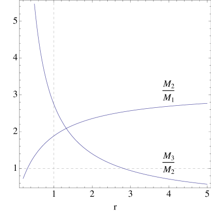
Note that r=1𝑟1r=1 corresponds to universal gaugino masses. Largely non universal masses can arise for r1𝑟1r\neq 1, despite SO(10)𝑆𝑂10SO(10) unification, as will be discussed in more detail in section 3.3. As a consequence, i) small values of r𝑟r can make the Wino lighter than the Bino and ii) the measurement of non-universal gaugino masses satisfying the sum rule (12) can be considered as another smoking gun of minimal unified TGM. The dependence of the gaugino mass parameter ratios M2/M1subscript𝑀2subscript𝑀1M_{2}/M_{1} and M3/M2subscript𝑀3subscript𝑀2M_{3}/M_{2} on r𝑟r at the SUSY breaking scale scale is shown in figure 2.
Refer to caption
Figure 2: Dependence of the gaugino mass parameter ratios M2/M1subscript𝑀2subscript𝑀1M_{2}/M_{1} and M3/M2subscript𝑀3subscript𝑀2M_{3}/M_{2} evaluated at the SUSY breaking scale on the parameter r𝑟r. The wino mass term M2subscript𝑀2M_{2} is lighter than the bino mass term M1subscript𝑀1M_{1} for r0.3less-than-or-similar-to𝑟0.3r\lesssim 0.3.

As usual, tanβ𝛽\tan\beta can be traded for the B𝐵B parameter in eq. (5) and sign(μ)sign𝜇\text{sign}(\mu), together with the EWSB condition, determine the μ𝜇\mu parameter.

Eqs. (7,8,1012) determine the boundary conditions of all the soft parameters except the MSSM A𝐴A-terms and the parameters of TGMAsubscriptsuperscript𝐴TGM\mathcal{L}^{A}_{\text{TGM}}. The latter, as the heavy field soft terms, are not relevant in our results. The MSSM A𝐴A-terms are instead of course relevant. Usually in gauge mediation it is assumed that the visible sector has only gauge interactions with the hidden sector and hence no A𝐴A-terms are generated at the one-loop level. This is not the case in unified TGM, where the MSSM fields and the minimal gauge mediation messengers lie in the same SO(10)𝑆𝑂10SO(10) multiplets, so that the messenger-messenger-Z𝑍Z coupling generating gaugino masses are accompanied by matter-messenger-Z𝑍Z couplings generating non-vanishing A𝐴A-terms at the messenger scale. Such A𝐴A-terms are rather model-dependent, as their values depend in the detailed form of the SO(10)𝑆𝑂10SO(10) lagrangian and on the implementation of doublet-triplet splitting in the Higgs sector. We will specify the prescription we use for the A𝐴A-terms in section 3.4.

3.2 Heavy chiral messengers and marginal parameters

In this subsection and in the next ones, we provide the details of the determination of the spectrum in terms of the relevant parameters and introduce additional physical parameters that have a marginal effect on the spectrum.

Let us begin with the scale M𝑀M at which the U(1)X𝑈subscript1𝑋U(1)_{X} subgroup of SO(10)𝑆𝑂10SO(10) is broken and the sfermion masses are generated, and their RGE evolution begins, which is expected to lie near the GUT scale. The TeV-scale predictions have only a mild (logarithmic) dependence on the precise value of M𝑀M. We therefore set M=MGUT𝑀subscript𝑀GUTM=M_{\text{GUT}} in our numerical results.

The spectrum below the GUT scale contains the MSSM fields and the extra heavy fields Dc+Dc¯superscript𝐷𝑐¯superscript𝐷𝑐D^{c}+\overline{D^{c}} and L+L¯𝐿¯𝐿L+\overline{L}. Such fields play an important role in the determination of the TeV-scale lagrangian. In fact, their coupling to supersymmetry breaking generates gaugino masses at the one loop. Moreover, their presence at high scale affects the running of the MSSM parameters. In order to compute the low energy spectrum, it is therefore necessary to know their masses and their couplings to supersymmetry breaking and MSSM fields.

Since the Dc,Lsuperscript𝐷𝑐𝐿D^{c},L and Dc¯,L¯¯superscript𝐷𝑐¯𝐿\overline{D^{c}},\overline{L} fields belong to different SO(10)𝑆𝑂10SO(10) representations, they acquire masses through SO(10)𝑆𝑂10SO(10) breaking, specifically through the vev of the SM singlet components of a 𝟏𝟔+𝟏𝟔¯16¯16\mathbf{16}+\overline{\mathbf{16}}, denoted by M>0𝑀0M>0333The D𝐷D-term condition for the U(1)X𝑈subscript1𝑋U(1)_{X} forces the two vevs to be equal in absolute value, up to negligible SUSY breaking effects. M𝑀M can be taken positive without loss of generality.. We expect M𝑀M to be of the order of the GUT scale, MMGUTsimilar-to𝑀subscript𝑀GUTM\sim M_{\text{GUT}} and denote by rGUTM/MGUTsubscript𝑟GUT𝑀subscript𝑀GUTr_{\text{GUT}}\equiv M/M_{\text{GUT}} their 𝒪(1)𝒪1\mathcal{O}\left(1\right) ratio. It is therefore convenient to write the mass terms in eq. (3) as

MijDDc¯iDjc+MijLL¯iLj=hijDMDc¯iDjc+hijLML¯iLj.subscriptsuperscript𝑀𝐷𝑖𝑗subscript¯superscript𝐷𝑐𝑖subscriptsuperscript𝐷𝑐𝑗subscriptsuperscript𝑀𝐿𝑖𝑗subscript¯𝐿𝑖subscript𝐿𝑗subscriptsuperscript𝐷𝑖𝑗𝑀subscript¯superscript𝐷𝑐𝑖subscriptsuperscript𝐷𝑐𝑗subscriptsuperscript𝐿𝑖𝑗𝑀subscript¯𝐿𝑖subscript𝐿𝑗M^{D}_{ij}\overline{D^{c}}_{i}D^{c}_{j}+M^{L}_{ij}\overline{L}_{i}L_{j}=h^{D}_{ij}M\overline{D^{c}}_{i}D^{c}_{j}+h^{L}_{ij}M\overline{L}_{i}L_{j}\,. (13)

The couplings hDsubscript𝐷h_{D}, hLsubscript𝐿h_{L} arise from the SO(10)𝑆𝑂10SO(10) superpotential [1, 2]

W2=hij𝟏𝟔i𝟏𝟎j𝟏𝟔+hij𝟏𝟔i𝟏𝟎j𝟏𝟔+yij2𝟏𝟔i𝟏𝟔j𝟏𝟎+W2NRsubscript𝑊2subscript𝑖𝑗subscript16𝑖subscript10𝑗16subscriptsuperscript𝑖𝑗subscript16𝑖subscript10𝑗superscript16subscript𝑦𝑖𝑗2subscript16𝑖subscript16𝑗10superscriptsubscript𝑊2NRW_{2}=h_{ij}\mathbf{16}_{i}\mathbf{10}_{j}\mathbf{16}+h^{\prime}_{ij}\mathbf{16}_{i}\mathbf{10}_{j}\mathbf{16}^{\prime}+\frac{y_{ij}}{2}\mathbf{16}_{i}\mathbf{16}_{j}\mathbf{10}+W_{2}^{\text{NR}} (14)

after substituting the vevs of the 𝟏𝟔16\mathbf{16}. In the SO(10)𝑆𝑂10SO(10) limit, hD=hL=hsubscript𝐷subscript𝐿h_{D}=h_{L}=h. Corrections to the above relations can originate from the non-renormalizable part of the superpotential, W2NRsuperscriptsubscript𝑊2NRW_{2}^{\text{NR}}. From eq. (14) it also follows that the mixing parameters MdDsubscript𝑀𝑑𝐷M_{dD} and MlLsubscript𝑀𝑙𝐿M_{lL} in eq. (3) vanish at the GUT scale at the renormalizable level, and are therefore set to zero at that scale:

MdD=0,MlL=0(GUT scale).formulae-sequencesubscript𝑀𝑑𝐷0subscript𝑀𝑙𝐿0(GUT scale)M_{dD}=0,\qquad M_{lL}=0\qquad\text{(GUT scale)}\,. (15)

Non vanishing values are generated by the RGE running between the GUT and the messenger scales, as no unbroken quantum number distinguishes the dc,lsuperscript𝑑𝑐𝑙d^{c},l fields from the Dc,Lsuperscript𝐷𝑐𝐿D^{c},L ones.

Supersymmetry breaking must be provided by the F𝐹F-term vev of the SM singlet component of spinorial representations of SO(10)𝑆𝑂10SO(10), which are however forced by gauge invariance not to coincide with 𝟏𝟔16\mathbf{16}, 𝟏𝟔¯¯16\overline{\mathbf{16}} (see the discussion in [2]) and will therefore be denoted by 𝟏𝟔superscript16\mathbf{16}^{\prime}, 𝟏𝟔¯superscript¯16\overline{\mathbf{16}}^{\prime}. In order to obtain positive tree level sfermion masses, the F𝐹F-term of the 𝟏𝟔superscript16\mathbf{16}^{\prime} must be larger than the one of the 𝟏𝟔¯superscript¯16\overline{\mathbf{16}}^{\prime} [2]. We will then assume for simplicity that only the SM singlet component of the 𝟏𝟔superscript16\mathbf{16}^{\prime} field, Z𝑍Z, gets an F𝐹F-term vev F𝐹F. As |F|M2much-less-than𝐹superscript𝑀2|F|\ll M^{2}, the field Z𝑍Z should be included in the effective lagrangian below the GUT scale defined by equations (25). The relevant terms are the superpotential couplings

WZ=hijDZDc¯iDjc+hijLZL¯iLj.subscript𝑊𝑍subscriptsuperscript𝐷𝑖𝑗𝑍subscript¯superscript𝐷𝑐𝑖subscriptsuperscript𝐷𝑐𝑗subscriptsuperscript𝐿𝑖𝑗𝑍subscript¯𝐿𝑖subscript𝐿𝑗W_{Z}=h^{\prime D}_{ij}Z\overline{D^{c}}_{i}D^{c}_{j}+h^{\prime L}_{ij}Z\overline{L}_{i}L_{j}\,. (16)

The couplings hDsubscriptsuperscript𝐷h^{\prime}_{D}, hLsubscriptsuperscript𝐿h^{\prime}_{L} arise from the SO(10)𝑆𝑂10SO(10) superpotential in eq. (14) after substituting the F𝐹F-term vev of 𝟏𝟔superscript16\mathbf{16}^{\prime}. In the SO(10)𝑆𝑂10SO(10) limit, hD=hL=hsubscriptsuperscript𝐷subscriptsuperscript𝐿superscripth^{\prime}_{D}=h^{\prime}_{L}=h^{\prime}. For simplicity, we will neglect the flavour structure of the matrices hDsubscript𝐷h_{D}, hLsubscript𝐿h_{L}, hDsubscriptsuperscript𝐷h^{\prime}_{D}, hLsubscriptsuperscript𝐿h^{\prime}_{L} and consider only the diagonal elements, assuming that, as in the case of the SM Yukawa couplings, the deviation from the diagonal form, i.e. the breaking of the individual flavour numbers, is small. In such a case, the flavour structure we are neglecting does not significantly affect the collider observables we are interested in. Eqs. (13) and (16) then involve six new parameters each. The latter are related to the MSSM down quark and charged lepton Yukawa couplings, as discussed in detail in appendix A. As shown there, the simplest possible prediction for the messenger mass parameters hD,Lsubscript𝐷𝐿h_{D,L}, which arises in the hypothesis of minimal Higgs embedding, 𝟏𝟔H=𝟏𝟔subscript16𝐻16\mathbf{16}_{H}=\mathbf{16}, is that they are proportional to the corresponding SM Yukawa couplings (in the presence of heavy Higgs triplets, this hypothesis gives rise to a predictive scheme for leptogenesis [7]):

hD=λD/sinθdhL=λE/sinθd.formulae-sequencesubscript𝐷subscript𝜆𝐷subscript𝜃𝑑subscript𝐿subscript𝜆𝐸subscript𝜃𝑑h_{D}=\lambda_{D}/\sin\theta_{d}\qquad h_{L}=\lambda_{E}/\sin\theta_{d}. (17)

We expect in this case the couplings hDi,Lisubscriptsubscript𝐷𝑖subscript𝐿𝑖h_{D_{i},L_{i}}, and therefore the messenger masses, to follow the same hierarchy as the corresponding fermion masses, with the first two family of messenger significantly lighter than the third one. The prediction in eq. (17), however, can receive corrections if the light Higgs fields have also a component in the 𝟏𝟔superscript16\mathbf{16}^{\prime}, 𝟏𝟔¯superscript¯16\overline{\mathbf{16}}^{\prime}. Moreover, the SO(10)𝑆𝑂10SO(10) relations between SM fermion and messenger couplings in eqs. (17) might receive corrections from the same sources of SO(10)𝑆𝑂10SO(10) breaking needed to fix the GUT prediction for the light fermion mass ratios, i.e. to differentiate λDsubscript𝜆𝐷\lambda_{D} and λETsubscriptsuperscript𝜆𝑇𝐸\lambda^{T}_{E}. In order to be general, we therefore modify the relations in eqs. (17) by introducing new parameters cDisubscript𝑐subscript𝐷𝑖c_{D_{i}}, cLisubscript𝑐subscript𝐿𝑖c_{L_{i}}, i=1,2,3𝑖123i=1,2,3,

hiD=cDiλiD/sinθdhiL=cLiλiL/sinθd,formulae-sequencesubscriptsuperscript𝐷𝑖subscript𝑐subscript𝐷𝑖subscriptsuperscript𝜆𝐷𝑖subscript𝜃𝑑subscriptsuperscript𝐿𝑖subscript𝑐subscript𝐿𝑖subscriptsuperscript𝜆𝐿𝑖subscript𝜃𝑑h^{D}_{i}=c_{D_{i}}\lambda^{D}_{i}/\sin\theta_{d}\qquad h^{L}_{i}=c_{L_{i}}\lambda^{L}_{i}/\sin\theta_{d}, (18)

whose relation with the fundamental parameters of the theory is discussed in Appendix A. The choice cDi,Li=1subscript𝑐subscript𝐷𝑖subscript𝐿𝑖1c_{D_{i},L_{i}}=1 in eq. (18) corresponds to the minimal setting in eqs. (17). We have checked that our TeV scale predictions have a very mild (logarithmic) dependence on 𝒪(1)𝒪1\mathcal{O}\left(1\right) variations of the parameters cDi,Lisubscript𝑐subscript𝐷𝑖subscript𝐿𝑖c_{D_{i},L_{i}}. Therefore, we set them to a reference value of 0.1 in most of the numerical results below, while keeping the possibility to give them an arbitrary value in our codes.

As for the couplings to supersymmetry breaking hDisubscriptsuperscriptsubscript𝐷𝑖h^{\prime}_{D_{i}} and hLisubscriptsuperscriptsubscript𝐿𝑖h^{\prime}_{L_{i}}, they are conveniently traded for the parameters γDisubscript𝛾subscript𝐷𝑖\gamma_{D_{i}}, γLisubscript𝛾subscript𝐿𝑖\gamma_{L_{i}} defined by

γDi(hDihDi)MDiγLi(hLihLi)MLi,formulae-sequencesubscript𝛾subscript𝐷𝑖subscriptsubscriptsuperscriptsubscript𝐷𝑖subscriptsubscript𝐷𝑖subscript𝑀subscript𝐷𝑖subscript𝛾subscript𝐿𝑖subscriptsubscriptsuperscriptsubscript𝐿𝑖subscriptsubscript𝐿𝑖subscript𝑀subscript𝐿𝑖\gamma_{D_{i}}\equiv\left(\frac{h^{\prime}_{D_{i}}}{h_{D_{i}}}\right)_{M_{D_{i}}}\qquad\gamma_{L_{i}}\equiv\left(\frac{h^{\prime}_{L_{i}}}{h_{L_{i}}}\right)_{M_{L_{i}}}, (19)

where the couplings are supposed to be evaluated at the corresponding heavy field mass scale MDi=hDiMsubscript𝑀subscript𝐷𝑖subscriptsubscript𝐷𝑖𝑀M_{D_{i}}=h_{D_{i}}M, MLi=hLiMsubscript𝑀subscript𝐿𝑖subscriptsubscript𝐿𝑖𝑀M_{L_{i}}=h_{L_{i}}M. In the next section we will show how the above parameters enter the determination of gaugino masses. For the time being, it suffices to note that the 6 parameters γDisubscript𝛾subscript𝐷𝑖\gamma_{D_{i}}, γLisubscript𝛾subscript𝐿𝑖\gamma_{L_{i}}, and therefore the couplings hDisubscriptsuperscriptsubscript𝐷𝑖h^{\prime}_{D_{i}}, hLisubscriptsuperscriptsubscript𝐿𝑖h^{\prime}_{L_{i}}, are determined in terms of M1/2subscript𝑀12M_{1/2}, r𝑟r (which determine, as we will see, the two averages γD(i=13γDi)/3subscript𝛾𝐷superscriptsubscript𝑖13subscript𝛾subscript𝐷𝑖3\gamma_{D}\equiv(\sum_{i=1}^{3}\gamma_{D_{i}})/3 and γL(i=13γLi)/3subscript𝛾𝐿superscriptsubscript𝑖13subscript𝛾subscript𝐿𝑖3\gamma_{L}\equiv(\sum_{i=1}^{3}\gamma_{L_{i}})/3), and the four ratios

rDi=γDi/γD,rLi=γLi/γL,i=1,2.formulae-sequencesubscript𝑟subscript𝐷𝑖subscript𝛾subscript𝐷𝑖subscript𝛾𝐷formulae-sequencesubscript𝑟subscript𝐿𝑖subscript𝛾subscript𝐿𝑖subscript𝛾𝐿𝑖12r_{D_{i}}=\gamma_{D_{i}}/\gamma_{D},\quad r_{L_{i}}=\gamma_{L_{i}}/\gamma_{L},\quad i=1,2. (20)

Again, the four parameters rDi,rLisubscript𝑟subscript𝐷𝑖subscript𝑟subscript𝐿𝑖r_{D_{i}},r_{L_{i}} can be expected to be of order one and we have checked that our TeV scale predictions have a very mild dependence on 𝒪(1)𝒪1\mathcal{O}\left(1\right) variations of those parameters. Therefore, we set them to 1, unless otherwise stated, in the numerical results below, while keeping the possibility to give them an arbitrary value in our codes.

The Yukawa couplings λ^Dsubscript^𝜆𝐷\hat{\lambda}_{D} and λ^Esubscript^𝜆𝐸\hat{\lambda}_{E} in eq. (3) are related to the up-type quark Yukawa couplings by the relations

λ^D=λ^E=cosθdcosθuλUsubscript^𝜆𝐷subscript^𝜆𝐸subscript𝜃𝑑subscript𝜃𝑢subscript𝜆𝑈\hat{\lambda}_{D}=\hat{\lambda}_{E}=\frac{\cos\theta_{d}}{\cos\theta_{u}}\lambda_{U} (21)

at the GUT scale, where we neglected possible contributions from non-renormalizable operators, as they are liklely to only affect the small couplings of the first two families, which are not relevant for our purposes.

To sum up, in this section we have specified the GUT scale boundary conditions for all the parameters in eq. (3). The Yukawas λUsubscript𝜆𝑈\lambda_{U}, λDsubscript𝜆𝐷\lambda_{D}, λEsubscript𝜆𝐸\lambda_{E} are determined at low energy by the SM fermion masses, and λ^Dsubscript^𝜆𝐷\hat{\lambda}_{D}, λ^Esubscript^𝜆𝐸\hat{\lambda}_{E} from GUT scale relations. The messenger masses MD,Lsubscript𝑀𝐷𝐿M_{D,L} are specified by eqs. (13,18) while the parameters MdDsubscript𝑀𝑑𝐷M_{dD}, MlLsubscript𝑀𝑙𝐿M_{lL} are set to zero at the GUT scale. The μ𝜇\mu parameter is determined by the EWSB condition and the specification of its sign. The parameters in eq. (16) will be determined in the next section by eqs. (19,20,25,26) together with eq. (11).

3.3 Gaugino masses in greater detail

In the remainder of this section, we will discuss in greater detail the determination of the soft terms.

As mentioned, gaugino masses are generated, as in minimal gauge mediation (MGM), at the one loop level because of the coupling of the supersymmetry breaking field Z𝑍Z to the heavy Dcsuperscript𝐷𝑐D^{c}, Dc¯¯superscript𝐷𝑐\overline{D^{c}}, L𝐿L and L¯¯𝐿\overline{L} fields, which play the role of chiral messengers of SUSY breaking.

While in MGM both the supersymmetric and supersymmetry breaking messenger masses come from the same Yukawa couplings, the ones to the spurion, here they are associated to two independent sets of couplings, the ones to U(1)X𝑈subscript1𝑋U(1)_{X} breaking, hD,Lsubscript𝐷𝐿h_{D,L}, and the ones to supersymmetry breaking, hD,Lsubscriptsuperscript𝐷𝐿h^{\prime}_{D,L}. This opens the possibility to enhance gaugino masses by means of the ratio of the couplings. In this section we show how such features are implemented in the SO(10)𝑆𝑂10SO(10) model under consideration, taking into account possible SO(10)𝑆𝑂10SO(10) breaking effects, and we point out a possible source of non minimality of gaugino masses, accounted for by the parameter r𝑟r in eq. (6).

Gaugino masses can be expressed in terms of the messenger masses and couplings to SUSY breaking in eqs. (13) and (16). The six vectorlike chiral messengers, Dic¯+Dic¯superscriptsubscript𝐷𝑖𝑐subscriptsuperscript𝐷𝑐𝑖\overline{D_{i}^{c}}+D^{c}_{i} and L¯i+Lisubscript¯𝐿𝑖subscript𝐿𝑖\overline{L}_{i}+L_{i}, i=1,2,3𝑖123i=1,2,3, have masses MDi=hDiMsubscript𝑀subscript𝐷𝑖subscriptsubscript𝐷𝑖𝑀M_{D_{i}}={h_{D}}_{i}M and MLi=hLiMsubscript𝑀subscript𝐿𝑖subscriptsubscript𝐿𝑖𝑀M_{L_{i}}={h_{L}}_{i}M respectively. Their scalar components get supersymmetry breaking mass terms given by hDiFsubscriptsuperscriptsubscript𝐷𝑖𝐹{h_{D}^{\prime}}_{i}F and hLiFsubscriptsuperscriptsubscript𝐿𝑖𝐹{h_{L}^{\prime}}_{i}F. The contributions of the i𝑖i-th family of messengers to the gaugino masses Masubscript𝑀𝑎M_{a}, a=1,2,3𝑎123a=1,2,3, are then

MaDi=αa(MDi)4πbaDγDiFM(scale MDi)MaLi=αa(MLi)4πbaLγLiFM(scale MLi),formulae-sequencesubscriptsuperscript𝑀subscript𝐷𝑖𝑎subscript𝛼𝑎subscript𝑀subscript𝐷𝑖4𝜋subscriptsuperscript𝑏𝐷𝑎subscriptsubscript𝛾𝐷𝑖𝐹𝑀(scale MDi)subscriptsuperscript𝑀subscript𝐿𝑖𝑎subscript𝛼𝑎subscript𝑀subscript𝐿𝑖4𝜋subscriptsuperscript𝑏𝐿𝑎subscriptsubscript𝛾𝐿𝑖𝐹𝑀(scale MLi)M^{D_{i}}_{a}=\frac{\alpha_{a}(M_{D_{i}})}{4\pi}b^{D}_{a}{\gamma_{D}}_{i}\frac{F}{M}\quad\text{(scale $M_{D_{i}}$)}\quad M^{L_{i}}_{a}=\frac{\alpha_{a}(M_{L_{i}})}{4\pi}b^{L}_{a}{\gamma_{L}}_{i}\frac{F}{M}\quad\text{(scale $M_{L_{i}}$)}, (22)

where bD=(2/5,0,1)superscript𝑏𝐷2501b^{D}=(2/5,0,1), bL=(3/5,1,0)superscript𝑏𝐿3510b^{L}=(3/5,1,0), and the parameters γDi,γLisubscriptsubscript𝛾𝐷𝑖subscriptsubscript𝛾𝐿𝑖{\gamma_{D}}_{i},{\gamma_{L}}_{i} are defined in eq. (19). Each of those contributions arise at the scale of the corresponding messenger and the gauge couplings in eqs. (22) are supposed to be evaluated at that scale, which is different for each contribution. The individual contributions in eqs. (22) can be formally obtained from the one loop running from the GUT scale of the hypothetical values

MaDi=αa(MGUT)4πbaDγDiFMMaLi=αa(MGUT)4πbaLγLiFM(GUT scale),formulae-sequencesubscriptsuperscript𝑀subscript𝐷𝑖𝑎subscript𝛼𝑎subscript𝑀GUT4𝜋subscriptsuperscript𝑏𝐷𝑎subscriptsubscript𝛾𝐷𝑖𝐹𝑀subscriptsuperscript𝑀subscript𝐿𝑖𝑎subscript𝛼𝑎subscript𝑀GUT4𝜋subscriptsuperscript𝑏𝐿𝑎subscriptsubscript𝛾𝐿𝑖𝐹𝑀(GUT scale)M^{D_{i}}_{a}=\frac{\alpha_{a}(M_{\text{GUT}})}{4\pi}b^{D}_{a}{\gamma_{D}}_{i}\frac{F}{M}\qquad M^{L_{i}}_{a}=\frac{\alpha_{a}(M_{\text{GUT}})}{4\pi}b^{L}_{a}{\gamma_{L}}_{i}\frac{F}{M}\quad\text{(GUT scale)}, (23)

where now the gauge couplings are supposed to be evaluated at the GUT scale, while γDsubscript𝛾𝐷\gamma_{D} and γLsubscript𝛾𝐿\gamma_{L} are still given by eq. (19). At the GUT scale, the individual contributions in eqs. (23) can be summed to give

Ma=3αa(MGUT)4π(2baD+rbaL1+r)γFM(GUT scale),subscript𝑀𝑎3subscript𝛼𝑎subscript𝑀GUT4𝜋2subscriptsuperscript𝑏𝐷𝑎𝑟subscriptsuperscript𝑏𝐿𝑎1𝑟𝛾𝐹𝑀(GUT scale)M_{a}=3\frac{\alpha_{a}(M_{\text{GUT}})}{4\pi}\left(2\frac{b^{D}_{a}+rb^{L}_{a}}{1+r}\right)\gamma\frac{F}{M}\quad\text{(GUT scale)}, (24)

where r𝑟r is a ratio and γ𝛾\gamma is the average of the six parameters defined in eq. (19):

r=i=13γLii=13γDi,γ=16(i=13γDi+i=13γLi).formulae-sequence𝑟superscriptsubscript𝑖13subscriptsubscript𝛾𝐿𝑖superscriptsubscript𝑖13subscriptsubscript𝛾𝐷𝑖𝛾16superscriptsubscript𝑖13subscriptsubscript𝛾𝐷𝑖superscriptsubscript𝑖13subscriptsubscript𝛾𝐿𝑖r=\frac{\sum_{i=1}^{3}{\gamma_{L}}_{i}}{\sum_{i=1}^{3}{\gamma_{D}}_{i}}\,,\qquad\gamma=\frac{1}{6}\bigg{(}\sum_{i=1}^{3}{\gamma_{D}}_{i}+\sum_{i=1}^{3}{\gamma_{L}}_{i}\bigg{)}\,. (25)

We can conveniently trade the parameter γ𝛾\gamma in terms of the more useful444If gauge couplings do not unify one should use (α2(MGUT)+α3(MGUT))/2subscript𝛼2subscript𝑀GUTsubscript𝛼3subscript𝑀GUT2(\alpha_{2}(M_{\text{GUT}})+\alpha_{3}(M_{\text{GUT}}))/2 instead of αGUTsubscript𝛼GUT\alpha_{\text{GUT}}.

M1/23αGUT4πγFM,subscript𝑀123subscript𝛼GUT4𝜋𝛾𝐹𝑀M_{1/2}\equiv 3\,\frac{\alpha_{\text{GUT}}}{4\pi}\gamma\frac{F}{M}\,, (26)

and thus obtain the parameterization of gaugino masses in terms of M1/2subscript𝑀12M_{1/2} and r𝑟r in eqs. (11) and the sum rule in eq. (12). As stressed above, those relations are valid at the GUT scale only in the sense that the gaugino masses at the scales at which they are actually generated and below can be obtained by running the formal GUT scale values with one loop RGEs.

The gaugino mass parameters M1/2subscript𝑀12M_{1/2} can well be of the order of the tree level stop mass m10subscript𝑚10m_{10}, despite it is generated at the one loop level [1]. This is in part due to the fact that F/M=10m10𝐹𝑀10subscript𝑚10F/M=\sqrt{10}\,m_{10}, giving a factor 3103103\sqrt{10} enhancement of the loop suppressed value

M1/2αGUT4π(310γ)m10.subscript𝑀12subscript𝛼GUT4𝜋310𝛾subscript𝑚10M_{1/2}\equiv\frac{\alpha_{\text{GUT}}}{4\pi}(3\sqrt{10}\,\gamma)m_{10}\,. (27)

And it is in part due to the fact that the unknown factor γ𝛾\gamma, being essentially a ratio of presumably hierarchical Yukawa couplings, can easily be larger (or smaller) than 1.

The gaugino masses obtained in this way are potentially non universal at the GUT scale, without any conflict with gauge coupling unification, if the parameter r𝑟r is different from 1. Let us close this section by discussing how concrete is such a possibility. The SU(5)𝑆𝑈5SU(5) gauge symmetry, if unbroken, would force γDi=γLisubscriptsubscript𝛾𝐷𝑖subscriptsubscript𝛾𝐿𝑖{\gamma_{D}}_{i}={\gamma_{L}}_{i} and r=1𝑟1r=1. On the other hand, the possibility that r1𝑟1r\neq 1 is plausible because SU(5)𝑆𝑈5SU(5) is broken and the same SU(5)𝑆𝑈5SU(5) breaking corrections needed to make λDλEsubscript𝜆𝐷subscript𝜆𝐸\lambda_{D}\neq\lambda_{E} can as well make hDhLsubscript𝐷subscript𝐿h_{D}\neq h_{L} and hDhLsubscriptsuperscript𝐷subscriptsuperscript𝐿h^{\prime}_{D}\neq h^{\prime}_{L}, so that γDiγLisubscriptsubscript𝛾𝐷𝑖subscriptsubscript𝛾𝐿𝑖{\gamma_{D}}_{i}\neq{\gamma_{L}}_{i} and r1𝑟1r\neq 1. Note that even in the limit in which the SU(5)𝑆𝑈5SU(5) breaking effects are small and only affect significantly the small Yukawa couplings of the first families, the effect on r𝑟r can be sizeable. In fact, the ratio of the small Yukawa couplings, potentially significantly different from 1, enters the r𝑟r parameter with the same weight as the ratio of the third family Yukawas.

3.4 Trilinear terms

The MSSM trilinear terms in eq. (5) are generated through one loop graphs at the scale at which the heavy Dcsuperscript𝐷𝑐D^{c}, Dc¯¯superscript𝐷𝑐\overline{D^{c}}, L𝐿L and L¯¯𝐿\overline{L} are integrated out. In the region of the parameter space where the messenger masses are well below the GUT scale, the loops generating the A𝐴A-terms are dominated by the contribution of the messengers, with the contribution of fields living at the GUT scale suppressed by their higher mass. In such a scase, the trilinears have the following form

AUsubscript𝐴𝑈\displaystyle A_{U} =AucλU+λUAq+λUAhu,absentsubscript𝐴superscript𝑢𝑐subscript𝜆𝑈subscript𝜆𝑈subscript𝐴𝑞subscript𝜆𝑈subscript𝐴subscript𝑢\displaystyle=A_{u^{c}}\lambda_{U}+\lambda_{U}A_{q}+\lambda_{U}A_{h_{u}}\;, (28)
ADsubscript𝐴𝐷\displaystyle A_{D} =AdcλD+λDAq+λDAhd,absentsubscript𝐴superscript𝑑𝑐subscript𝜆𝐷subscript𝜆𝐷subscript𝐴𝑞subscript𝜆𝐷subscript𝐴subscript𝑑\displaystyle=A_{d^{c}}\lambda_{D}+\lambda_{D}A_{q}+\lambda_{D}A_{h_{d}}\;,
AEsubscript𝐴𝐸\displaystyle A_{E} =AecλE+λEAl+λEAhd.absentsubscript𝐴superscript𝑒𝑐subscript𝜆𝐸subscript𝜆𝐸subscript𝐴𝑙subscript𝜆𝐸subscript𝐴subscript𝑑\displaystyle=A_{e^{c}}\lambda_{E}+\lambda_{E}A_{l}+\lambda_{E}A_{h_{d}}\;.

More precisely, the contributions induced by the coloured messengers Dcsuperscript𝐷𝑐D^{c} and Dc¯¯superscript𝐷𝑐\overline{D^{c}} are

Aq(MDi)subscript𝐴𝑞subscriptsubscript𝑀𝐷𝑖\displaystyle A_{q}({M_{D}}_{i}) =1(4π)2γDiλ^Di2FM,absent1superscript4𝜋2subscriptsubscript𝛾𝐷𝑖superscriptsubscript^𝜆subscript𝐷𝑖2𝐹𝑀\displaystyle=-\frac{1}{(4\pi)^{2}}{\gamma_{D}}_{i}{\hat{\lambda}_{D_{i}}}^{2}\,\frac{F}{M}\;, (29a)
Ahd(MDi)subscript𝐴subscript𝑑subscriptsubscript𝑀𝐷𝑖\displaystyle A_{h_{d}}({M_{D}}_{i}) =3(4π)2γDiλ^Di2FM,absent3superscript4𝜋2subscriptsubscript𝛾𝐷𝑖superscriptsubscript^𝜆subscript𝐷𝑖2𝐹𝑀\displaystyle=-\frac{3}{(4\pi)^{2}}{\gamma_{D}}_{i}{\hat{\lambda}_{D_{i}}}^{2}\,\frac{F}{M}\;, (29b)
Al(MDi)subscript𝐴𝑙subscriptsubscript𝑀𝐷𝑖\displaystyle A_{l}({M_{D}}_{i}) =Adc(MDi)=Auc(MDi)=Aec(MDi)=Ahu(MDi)=0,absentsubscript𝐴superscript𝑑𝑐subscriptsubscript𝑀𝐷𝑖subscript𝐴superscript𝑢𝑐subscriptsubscript𝑀𝐷𝑖subscript𝐴superscript𝑒𝑐subscriptsubscript𝑀𝐷𝑖subscript𝐴subscript𝑢subscriptsubscript𝑀𝐷𝑖0\displaystyle=A_{d^{c}}({M_{D}}_{i})=A_{u^{c}}({M_{D}}_{i})=A_{e^{c}}({M_{D}}_{i})=A_{h_{u}}({M_{D}}_{i})=0\;, (29c)

while the one induced by L𝐿L and L¯¯𝐿\overline{L} are

Aec(MLi)subscript𝐴superscript𝑒𝑐subscriptsubscript𝑀𝐿𝑖\displaystyle A_{e^{c}}({M_{L}}_{i}) =2(4π)2γLiλ^Ei2FM,absent2superscript4𝜋2subscriptsubscript𝛾𝐿𝑖superscriptsubscript^𝜆subscript𝐸𝑖2𝐹𝑀\displaystyle=-\frac{2}{(4\pi)^{2}}{\gamma_{L}}_{i}{\hat{\lambda}_{E_{i}}}^{2}\,\frac{F}{M}\;, (30a)
Ahd(MLi)subscript𝐴subscript𝑑subscriptsubscript𝑀𝐿𝑖\displaystyle A_{h_{d}}({M_{L}}_{i}) =1(4π)2γLiλ^Ei2FM,absent1superscript4𝜋2subscriptsubscript𝛾𝐿𝑖superscriptsubscript^𝜆subscript𝐸𝑖2𝐹𝑀\displaystyle=-\frac{1}{(4\pi)^{2}}{\gamma_{L}}_{i}{\hat{\lambda}_{E_{i}}}^{2}\,\frac{F}{M}\;, (30b)
Al(MLi)subscript𝐴𝑙subscriptsubscript𝑀𝐿𝑖\displaystyle A_{l}({M_{L}}_{i}) =Adc(MLi)=Auc(MLi)=Aq(MLi)=Ahu(MLi)=0.absentsubscript𝐴superscript𝑑𝑐subscriptsubscript𝑀𝐿𝑖subscript𝐴superscript𝑢𝑐subscriptsubscript𝑀𝐿𝑖subscript𝐴𝑞subscriptsubscript𝑀𝐿𝑖subscript𝐴subscript𝑢subscriptsubscript𝑀𝐿𝑖0\displaystyle=A_{d^{c}}({M_{L}}_{i})=A_{u^{c}}({M_{L}}_{i})=A_{q}({M_{L}}_{i})=A_{h_{u}}({M_{L}}_{i})=0\;. (30c)

Note that only the third family A𝐴A-terms are non negligible, as the first and second family ones are suppressed by powers of small Yukawa couplings. This solves the supersymmetric CP problem.

On the other hand, if tanβ𝛽\tan\beta is largish and/or θdsubscript𝜃𝑑\theta_{d} is small, the third family messenger masses can be close to the GUT scale. This possibility is particularly interesting, as it corresponds to third family Yukawa couplings of order 1 in the microscopic theory at the GUT scale. In fact, let us remind that MDi,LihDi,LiMhDi,LiMGUTsimilar-tosubscript𝑀subscript𝐷𝑖subscript𝐿𝑖subscriptsubscript𝐷𝑖subscript𝐿𝑖𝑀similar-tosubscriptsubscript𝐷𝑖subscript𝐿𝑖subscript𝑀GUTM_{D_{i},L_{i}}\sim h_{D_{i},L_{i}}M\sim h_{D_{i},L_{i}}M_{\text{GUT}}, with the third family expected to be largest. Therefore, MD3,L3MGUTsimilar-tosubscript𝑀subscript𝐷3subscript𝐿3subscript𝑀GUTM_{D_{3},L_{3}}\sim M_{\text{GUT}} requires hD3,L31similar-tosubscriptsubscript𝐷3subscript𝐿31h_{D_{3},L_{3}}\sim 1. In such a case, the suppression of the bottom and the tau mass compared to the top one is due either to a small vev of hdsubscript𝑑h_{d} (large tanβ𝛽\tan\beta) or a small component of hdsubscript𝑑h_{d} in 𝟏𝟔Hsubscript16𝐻\mathbf{16}_{H} (small θdsubscript𝜃𝑑\theta_{d}, see eq. (9)). This can be seen from eq. (18) with cD3,L31similar-tosubscript𝑐subscript𝐷3subscript𝐿31c_{D_{3},L_{3}}\sim 1, which gives mb,τ=vλb,τcosβvhb,τsinθdcosβvsinθdcosβsubscript𝑚𝑏𝜏𝑣subscript𝜆𝑏𝜏𝛽similar-to𝑣subscript𝑏𝜏subscript𝜃𝑑𝛽similar-to𝑣subscript𝜃𝑑𝛽m_{b,\tau}=v\lambda_{b,\tau}\cos\beta\sim vh_{b,\tau}\sin\theta_{d}\cos\beta\sim v\sin\theta_{d}\cos\beta, where v174GeV𝑣174GeVv\approx 174\,\mathrm{GeV}. From the point of view of the A𝐴A-terms, the case with the third family of messengers close to the GUT scale is interesting because the contribution to the A𝐴A-terms of fields with GUT scale masses is comparable to the one from the third family of messengers, and can significantly enhance them. For example, the SU(5)𝑆𝑈5SU(5) representations 𝟏𝟎10\mathbf{10} and 𝟏1\mathbf{1} in the 𝟏𝟔16\mathbf{16} or 𝟏𝟔superscript16\mathbf{16}^{\prime} will contribute to the A𝐴A-terms through their couplings to the matter fields in eq. (14).

As mentioned, the contribution of the GUT-scale fields to the A𝐴A-terms is quite model-dependent, as it depends on the detailed form of the SO(10)𝑆𝑂10SO(10) lagrangian and on the implementation of doublet-triplet splitting in the Higgs sector. Still, a realistic estimate can be obtained by using the renormalizable part of the superpotential in eq. (14) and by assuming that all the components in 𝟏𝟔16\mathbf{16} and 𝟏𝟔superscript16\mathbf{16}^{\prime} are at the same scale as the third family messengers. In such a case, the A𝐴A-terms can be written as (neglecting corrections from non-renormalizable operators)

AUsubscript𝐴𝑈\displaystyle A_{U} =AucλU+λUAq+λUAy(u),absentsubscript𝐴superscript𝑢𝑐subscript𝜆𝑈subscript𝜆𝑈subscript𝐴𝑞subscript𝜆𝑈subscriptsuperscript𝐴𝑢𝑦\displaystyle=A_{u^{c}}\lambda_{U}+\lambda_{U}A_{q}+\lambda_{U}A^{(u)}_{y}\;, (31a)
ADsubscript𝐴𝐷\displaystyle A_{D} =AdcλD+λDAq+λD(Ay(d)+Ah+Ah),absentsubscript𝐴superscript𝑑𝑐subscript𝜆𝐷subscript𝜆𝐷subscript𝐴𝑞subscript𝜆𝐷subscriptsuperscript𝐴𝑑𝑦subscript𝐴subscript𝐴superscript\displaystyle=A_{d^{c}}\lambda_{D}+\lambda_{D}A_{q}+\lambda_{D}(A^{(d)}_{y}+A_{h}+A_{h^{\prime}})\;, (31b)
AEsubscript𝐴𝐸\displaystyle A_{E} =AecλE+λEAl+λE(Ay(d)+Ah+Ah),absentsubscript𝐴superscript𝑒𝑐subscript𝜆𝐸subscript𝜆𝐸subscript𝐴𝑙subscript𝜆𝐸subscriptsuperscript𝐴𝑑𝑦subscript𝐴subscript𝐴superscript\displaystyle=A_{e^{c}}\lambda_{E}+\lambda_{E}A_{l}+\lambda_{E}(A^{(d)}_{y}+A_{h}+A_{h^{\prime}})\;, (31c)

where the individual contributions read

Aq(MDi)subscript𝐴𝑞subscript𝑀subscript𝐷𝑖\displaystyle A_{q}(M_{D_{i}}) =1(4π)2hihi(2(hi2+hi2)+yi2)FM,absent1superscript4𝜋2subscriptsuperscript𝑖subscript𝑖2superscriptsubscript𝑖2superscriptsubscriptsuperscript𝑖2superscriptsubscript𝑦𝑖2𝐹𝑀\displaystyle=-\frac{1}{(4\pi)^{2}}\frac{h^{\prime}_{i}}{h_{i}}\left(2\left({h_{i}}^{2}+{h^{\prime}_{i}}^{2}\right)+{y_{i}}^{2}\right)\frac{F}{M}\;, (32a)
Auc(MDi)subscript𝐴superscript𝑢𝑐subscript𝑀subscript𝐷𝑖\displaystyle A_{u^{c}}(M_{D_{i}}) =1(4π)2hihi(hi2+hi2+2yi2)FM,absent1superscript4𝜋2subscriptsuperscript𝑖subscript𝑖superscriptsubscript𝑖2superscriptsubscriptsuperscript𝑖22superscriptsubscript𝑦𝑖2𝐹𝑀\displaystyle=-\frac{1}{(4\pi)^{2}}\frac{h^{\prime}_{i}}{h_{i}}\left({h_{i}}^{2}+{h^{\prime}_{i}}^{2}+2{y_{i}}^{2}\right)\frac{F}{M}\;, (32b)
Adc(MDi)subscript𝐴superscript𝑑𝑐subscript𝑀subscript𝐷𝑖\displaystyle A_{d^{c}}(M_{D_{i}}) =1(4π)2hihi2(hi2+hi2)FM,absent1superscript4𝜋2subscriptsuperscript𝑖subscript𝑖2superscriptsubscript𝑖2superscriptsubscriptsuperscript𝑖2𝐹𝑀\displaystyle=-\frac{1}{(4\pi)^{2}}\frac{h^{\prime}_{i}}{h_{i}}2\left({h_{i}}^{2}+{h^{\prime}_{i}}^{2}\right)\frac{F}{M}\;, (32c)
Al(MDi)subscript𝐴𝑙subscript𝑀subscript𝐷𝑖\displaystyle A_{l}(M_{D_{i}}) =1(4π)2hihi3(hi2+hi2)FM,absent1superscript4𝜋2subscriptsuperscript𝑖subscript𝑖3superscriptsubscript𝑖2superscriptsubscriptsuperscript𝑖2𝐹𝑀\displaystyle=-\frac{1}{(4\pi)^{2}}\frac{h^{\prime}_{i}}{h_{i}}3\left({h_{i}}^{2}+{h^{\prime}_{i}}^{2}\right)\frac{F}{M}\;, (32d)
Aec(MDi)subscript𝐴superscript𝑒𝑐subscript𝑀subscript𝐷𝑖\displaystyle A_{e^{c}}(M_{D_{i}}) =1(4π)2hihi3(hi2+hi2)FM,absent1superscript4𝜋2subscriptsuperscript𝑖subscript𝑖3superscriptsubscript𝑖2superscriptsubscriptsuperscript𝑖2𝐹𝑀\displaystyle=-\frac{1}{(4\pi)^{2}}\frac{h^{\prime}_{i}}{h_{i}}3\left({h_{i}}^{2}+{h^{\prime}_{i}}^{2}\right)\frac{F}{M}\;, (32e)
Ay(d)(MDi)subscriptsuperscript𝐴𝑑𝑦subscript𝑀subscript𝐷𝑖\displaystyle A^{(d)}_{y}(M_{D_{i}}) =3(4π)2hihiyi2FM,absent3superscript4𝜋2subscriptsuperscript𝑖subscript𝑖superscriptsubscript𝑦𝑖2𝐹𝑀\displaystyle=-\frac{3}{(4\pi)^{2}}\frac{h^{\prime}_{i}}{h_{i}}{y_{i}}^{2}\,\frac{F}{M}\;, (32f)
Ay(u)(MDi)subscriptsuperscript𝐴𝑢𝑦subscript𝑀subscript𝐷𝑖\displaystyle A^{(u)}_{y}(M_{D_{i}}) =Ah(MDi)=Ah(MDi)=0,absentsubscript𝐴subscript𝑀subscript𝐷𝑖subscript𝐴superscriptsubscript𝑀subscript𝐷𝑖0\displaystyle=A_{h}(M_{D_{i}})=A_{h^{\prime}}(M_{D_{i}})=0\;, (32g)
Aq(MLi)subscript𝐴𝑞subscript𝑀subscript𝐿𝑖\displaystyle A_{q}(M_{L_{i}}) =1(4π)2hihi(hi2+hi2+yi2)FM,absent1superscript4𝜋2subscriptsuperscript𝑖subscript𝑖superscriptsubscript𝑖2superscriptsubscriptsuperscript𝑖2superscriptsubscript𝑦𝑖2𝐹𝑀\displaystyle=-\frac{1}{(4\pi)^{2}}\frac{h^{\prime}_{i}}{h_{i}}\left({h_{i}}^{2}+{h^{\prime}_{i}}^{2}+{y_{i}}^{2}\right)\frac{F}{M}\;, (32h)
Auc(MLi)subscript𝐴superscript𝑢𝑐subscript𝑀subscript𝐿𝑖\displaystyle A_{u^{c}}(M_{L_{i}}) =1(4π)2hihi2(hi2+hi2)FM,absent1superscript4𝜋2subscriptsuperscript𝑖subscript𝑖2superscriptsubscript𝑖2superscriptsubscriptsuperscript𝑖2𝐹𝑀\displaystyle=-\frac{1}{(4\pi)^{2}}\frac{h^{\prime}_{i}}{h_{i}}2\left({h_{i}}^{2}+{h^{\prime}_{i}}^{2}\right)\frac{F}{M}\;, (32i)
Adc(MLi)subscript𝐴superscript𝑑𝑐subscript𝑀subscript𝐿𝑖\displaystyle A_{d^{c}}(M_{L_{i}}) =1(4π)2hihi2(hi2+hi2)FM,absent1superscript4𝜋2subscriptsuperscript𝑖subscript𝑖2superscriptsubscript𝑖2superscriptsubscriptsuperscript𝑖2𝐹𝑀\displaystyle=-\frac{1}{(4\pi)^{2}}\frac{h^{\prime}_{i}}{h_{i}}2\left({h_{i}}^{2}+{h^{\prime}_{i}}^{2}\right)\frac{F}{M}\;, (32j)
Al(MLi)subscript𝐴𝑙subscript𝑀subscript𝐿𝑖\displaystyle A_{l}(M_{L_{i}}) =1(4π)2hihi(hi2+hi2)FM,absent1superscript4𝜋2subscriptsuperscript𝑖subscript𝑖superscriptsubscript𝑖2superscriptsubscriptsuperscript𝑖2𝐹𝑀\displaystyle=-\frac{1}{(4\pi)^{2}}\frac{h^{\prime}_{i}}{h_{i}}\left({h_{i}}^{2}+{h^{\prime}_{i}}^{2}\right)\frac{F}{M}\;, (32k)
Aec(MLi)subscript𝐴superscript𝑒𝑐subscript𝑀subscript𝐿𝑖\displaystyle A_{e^{c}}(M_{L_{i}}) =1(4π)2hihi 2yi2FM,absent1superscript4𝜋2subscriptsuperscript𝑖subscript𝑖2superscriptsubscript𝑦𝑖2𝐹𝑀\displaystyle=-\frac{1}{(4\pi)^{2}}\frac{h^{\prime}_{i}}{h_{i}}\,2{y_{i}}^{2}\frac{F}{M}\;, (32l)
Ay(d)(MLi)subscriptsuperscript𝐴𝑑𝑦subscript𝑀subscript𝐿𝑖\displaystyle A^{(d)}_{y}(M_{L_{i}}) =1(4π)2hihiyi2FM,absent1superscript4𝜋2subscriptsuperscript𝑖subscript𝑖superscriptsubscript𝑦𝑖2𝐹𝑀\displaystyle=-\frac{1}{(4\pi)^{2}}\frac{h^{\prime}_{i}}{h_{i}}{y_{i}}^{2}\frac{F}{M}\;, (32m)
Ay(u)(MLi)subscriptsuperscript𝐴𝑢𝑦subscript𝑀subscript𝐿𝑖\displaystyle A^{(u)}_{y}(M_{L_{i}}) =1(4π)2hihiyi2FM,absent1superscript4𝜋2subscriptsuperscript𝑖subscript𝑖superscriptsubscript𝑦𝑖2𝐹𝑀\displaystyle=-\frac{1}{(4\pi)^{2}}\frac{h^{\prime}_{i}}{h_{i}}{y_{i}}^{2}\frac{F}{M}\;, (32n)
Ah(MLi)subscript𝐴subscript𝑀subscript𝐿𝑖\displaystyle A_{h}(M_{L_{i}}) =1(4π)2hihihi2FM,absent1superscript4𝜋2subscriptsuperscript𝑖subscript𝑖superscriptsubscript𝑖2𝐹𝑀\displaystyle=-\frac{1}{(4\pi)^{2}}\frac{h^{\prime}_{i}}{h_{i}}{h_{i}}^{2}\frac{F}{M}\;, (32o)
Ah(MLi)subscript𝐴superscriptsubscript𝑀subscript𝐿𝑖\displaystyle A_{h^{\prime}}(M_{L_{i}}) =1(4π)2hihihi2FM.absent1superscript4𝜋2subscriptsuperscript𝑖subscript𝑖superscriptsubscriptsuperscript𝑖2𝐹𝑀\displaystyle=-\frac{1}{(4\pi)^{2}}\frac{h^{\prime}_{i}}{h_{i}}{h^{\prime}_{i}}^{2}\frac{F}{M}\;. (32p)

In our numerical analysis we will use for definiteness the above expressions.

3.5 Two loop level contributions to sfermion masses

The coupling of the chiral messengers Dcsuperscript𝐷𝑐D^{c}, Dc¯¯superscript𝐷𝑐\overline{D^{c}}, L𝐿L and L¯¯𝐿\overline{L} to SUSY breaking, eq. (16), gives rise to the well known MGM two loop contributions to sfermion masses. In this section we give their expressions in our model. As the chiral messengers have supersymmetric masses hDiMsubscriptsubscript𝐷𝑖𝑀h_{D_{i}}M and hLiMsubscriptsubscript𝐿𝑖𝑀h_{L_{i}}M and supersymmetry breaking mass terms given by hDiFsubscriptsuperscriptsubscript𝐷𝑖𝐹{h_{D}^{\prime}}_{i}F and hLiFsubscriptsuperscriptsubscript𝐿𝑖𝐹{h_{L}^{\prime}}_{i}F, the contributions to sfermion masses, as the ones to gaugino masses, depend on the parameters γDisubscriptsubscript𝛾𝐷𝑖{\gamma_{D}}_{i} and γLisubscriptsubscript𝛾𝐿𝑖{\gamma_{L}}_{i} and can be similarly ehanced. We have in fact

(mQ2)MGM=i(mQ2)MGM(MDi)+(mQ2)MGM(MLi)=2[(cQ(3)α32(MDi)(4π)2+25cQ(1)α12(MDi)(4π)2)γDi2+(cQ(2)α22(MLi)(4π)2+35cQ(1)α12(MLi)(4π)2)γLi2](FM)2,subscriptsubscriptsuperscript𝑚2𝑄MGMsubscript𝑖subscriptsubscriptsuperscript𝑚2𝑄MGMsubscriptsubscript𝑀𝐷𝑖subscriptsubscriptsuperscript𝑚2𝑄MGMsubscriptsubscript𝑀𝐿𝑖2delimited-[]subscriptsuperscript𝑐3𝑄superscriptsubscript𝛼32subscriptsubscript𝑀𝐷𝑖superscript4𝜋225subscriptsuperscript𝑐1𝑄superscriptsubscript𝛼12subscriptsubscript𝑀𝐷𝑖superscript4𝜋2superscriptsubscriptsubscript𝛾𝐷𝑖2subscriptsuperscript𝑐2𝑄superscriptsubscript𝛼22subscriptsubscript𝑀𝐿𝑖superscript4𝜋235subscriptsuperscript𝑐1𝑄superscriptsubscript𝛼12subscriptsubscript𝑀𝐿𝑖superscript4𝜋2superscriptsubscriptsubscript𝛾𝐿𝑖2superscript𝐹𝑀2\begin{split}(m^{2}_{Q})_{\text{MGM}}&=\sum_{i}(m^{2}_{Q})_{\text{MGM}}({M_{D}}_{i})+(m^{2}_{Q})_{\text{MGM}}({M_{L}}_{i})\\ &=2\bigg{[}\bigg{(}c^{(3)}_{Q}\frac{\alpha_{3}^{2}({M_{D}}_{i})}{(4\pi)^{2}}+\frac{2}{5}c^{(1)}_{Q}\frac{\alpha_{1}^{2}({M_{D}}_{i})}{(4\pi)^{2}}\bigg{)}{\gamma_{D}}_{i}^{2}\;\\ &\quad\,+\bigg{(}c^{(2)}_{Q}\frac{\alpha_{2}^{2}({M_{L}}_{i})}{(4\pi)^{2}}+\frac{3}{5}c^{(1)}_{Q}\frac{\alpha_{1}^{2}({M_{L}}_{i})}{(4\pi)^{2}}\bigg{)}{\gamma_{L}}_{i}^{2}\bigg{]}\left(\frac{F}{M}\right)^{2}\;,\\ \end{split} (33)

where cQ(a)subscriptsuperscript𝑐𝑎𝑄c^{(a)}_{Q} is the quadratic Casimir of the sfermion Q~~𝑄\widetilde{Q} (or Higgs Q𝑄Q) relative to the gauge interaction a𝑎a, as in Table 2. The parameters γDi,Li(F/M)subscript𝛾subscript𝐷𝑖subscript𝐿𝑖𝐹𝑀\gamma_{D_{i},L_{i}}(F/M) are determined by the parameters M1/2subscript𝑀12M_{1/2}, r𝑟r, rDi,rLisubscriptsubscript𝑟𝐷𝑖subscriptsubscript𝑟𝐿𝑖{r_{D}}_{i},{r_{L}}_{i}, i=1,2𝑖12i=1,2 through eqs. (20), (25) and (26).

Q𝑄Q qisubscript𝑞𝑖q_{i} uicsuperscriptsubscript𝑢𝑖𝑐u_{i}^{c} dicsuperscriptsubscript𝑑𝑖𝑐d_{i}^{c} lisubscript𝑙𝑖l_{i} eicsuperscriptsubscript𝑒𝑖𝑐e_{i}^{c} husubscript𝑢h_{u} hdsubscript𝑑h_{d}
cQ(1)subscriptsuperscript𝑐1𝑄c^{(1)}_{Q} 1/601601/60 4/154154/15 1/151151/15 3/203203/20 3/5353/5 3/203203/20 3/203203/20
cQ(2)subscriptsuperscript𝑐2𝑄c^{(2)}_{Q} 3/4343/4 00 00 3/4343/4 00 3/4343/4 3/4343/4
cQ(3)subscriptsuperscript𝑐3𝑄c^{(3)}_{Q} 4/3434/3 4/3434/3 4/3434/3 00 00 00 00
Table 2: Quadratic Casimirs for the low energy superfields.

On top of the usual MGM contributions, soft masses receive also two loop contributions because of messenger-matter mixing. Sizeable contributions arise only for third family sfermions (and Higgses). All in all the corrections are (remember that |F/M|2=10m102superscript𝐹𝑀210superscriptsubscript𝑚102|F/M|^{2}=10\,m_{10}^{2})

(4π)4δmq32=superscript4𝜋4𝛿subscriptsuperscript𝑚2subscript𝑞3absent\displaystyle(4\pi)^{4}\delta{m}^{2}_{q_{3}}= (730g12+32g22+83g323λ^D3212(λE32+λ^E32))λ^D32γD32(FM)2730superscriptsubscript𝑔1232superscriptsubscript𝑔2283superscriptsubscript𝑔323superscriptsubscript^𝜆subscript𝐷3212superscriptsubscript𝜆subscript𝐸32superscriptsubscript^𝜆subscript𝐸32superscriptsubscript^𝜆subscript𝐷32superscriptsubscript𝛾subscript𝐷32superscript𝐹𝑀2\displaystyle\left(\frac{7}{30}g_{1}^{2}+\frac{3}{2}g_{2}^{2}+\frac{8}{3}g_{3}^{2}-3\hat{\lambda}_{D_{3}}^{2}-\frac{1}{2}(\lambda_{E_{3}}^{2}+\hat{\lambda}_{E_{3}}^{2})\right)\hat{\lambda}_{D_{3}}^{2}\gamma_{D_{3}}^{2}\left(\frac{F}{M}\right)^{2}
+12λD32λ^E32γE32(FM)212superscriptsubscript𝜆subscript𝐷32superscriptsubscript^𝜆subscript𝐸32superscriptsubscript𝛾subscript𝐸32superscript𝐹𝑀2\displaystyle+\frac{1}{2}\lambda_{D_{3}}^{2}\hat{\lambda}_{E_{3}}^{2}\gamma_{E_{3}}^{2}\left(\frac{F}{M}\right)^{2} (34a)
(4π)4δml32=superscript4𝜋4𝛿subscriptsuperscript𝑚2subscript𝑙3absent\displaystyle(4\pi)^{4}\delta{m}^{2}_{l_{3}}= (32λ^D32λE32γD32+2λE32λ^E32γE32)(FM)232superscriptsubscript^𝜆subscript𝐷32superscriptsubscript𝜆subscript𝐸32superscriptsubscript𝛾subscript𝐷322superscriptsubscript𝜆subscript𝐸32superscriptsubscript^𝜆subscript𝐸32superscriptsubscript𝛾subscript𝐸32superscript𝐹𝑀2\displaystyle\left(\frac{3}{2}\hat{\lambda}_{D_{3}}^{2}\lambda_{E_{3}}^{2}\gamma_{D_{3}}^{2}+2\lambda_{E_{3}}^{2}\hat{\lambda}_{E_{3}}^{2}\gamma_{E_{3}}^{2}\right)\left(\frac{F}{M}\right)^{2} (34b)
(4π)4δmd2=superscript4𝜋4𝛿subscriptsuperscript𝑚2𝑑absent\displaystyle(4\pi)^{4}\delta{m}^{2}_{d}= (6λ^D32λD32γD32+λ^E32λD32γE32)(FM)26superscriptsubscript^𝜆subscript𝐷32superscriptsubscript𝜆subscript𝐷32superscriptsubscript𝛾subscript𝐷32superscriptsubscript^𝜆subscript𝐸32superscriptsubscript𝜆subscript𝐷32superscriptsubscript𝛾subscript𝐸32superscript𝐹𝑀2\displaystyle\left(6\hat{\lambda}_{D_{3}}^{2}\lambda_{D_{3}}^{2}\gamma_{D_{3}}^{2}+\hat{\lambda}_{E_{3}}^{2}\lambda_{D_{3}}^{2}\gamma_{E_{3}}^{2}\right)\left(\frac{F}{M}\right)^{2} (34c)
(4π)4δme32=superscript4𝜋4𝛿subscriptsuperscript𝑚2subscript𝑒3absent\displaystyle(4\pi)^{4}\delta{m}^{2}_{e_{3}}= (95g12+3g224λ^E323(λD32+λ^D32))λ^E32γE32(FM)295superscriptsubscript𝑔123superscriptsubscript𝑔224superscriptsubscript^𝜆subscript𝐸323superscriptsubscript𝜆subscript𝐷32superscriptsubscript^𝜆subscript𝐷32superscriptsubscript^𝜆subscript𝐸32superscriptsubscript𝛾subscript𝐸32superscript𝐹𝑀2\displaystyle\left(\frac{9}{5}g_{1}^{2}+3g_{2}^{2}-4\hat{\lambda}_{E_{3}}^{2}-3(\lambda_{D_{3}}^{2}+\hat{\lambda}_{D_{3}}^{2})\right)\hat{\lambda}_{E_{3}}^{2}\gamma_{E_{3}}^{2}\left(\frac{F}{M}\right)^{2}
+3λE32λ^D32γD32(FM)23superscriptsubscript𝜆subscript𝐸32superscriptsubscript^𝜆subscript𝐷32superscriptsubscript𝛾subscript𝐷32superscript𝐹𝑀2\displaystyle+3\lambda_{E_{3}}^{2}\hat{\lambda}_{D_{3}}^{2}\gamma_{D_{3}}^{2}\left(\frac{F}{M}\right)^{2} (34d)
(4π)4δmu32=superscript4𝜋4𝛿subscriptsuperscript𝑚2subscript𝑢3absent\displaystyle(4\pi)^{4}\delta{m}^{2}_{u_{3}}= (λU32λ^D32γD32)(FM)2superscriptsubscript𝜆subscript𝑈32superscriptsubscript^𝜆subscript𝐷32superscriptsubscript𝛾subscript𝐷32superscript𝐹𝑀2\displaystyle\left(\lambda_{U_{3}}^{2}\hat{\lambda}_{D_{3}}^{2}\gamma_{D_{3}}^{2}\right)\left(\frac{F}{M}\right)^{2} (34e)
(4π)4δmhd2=superscript4𝜋4𝛿subscriptsuperscript𝑚2subscript𝑑absent\displaystyle(4\pi)^{4}\delta{m}^{2}_{h_{d}}= (710g12+92g22+8g329λ^D3232(λ^E32+λU32))λ^D32γD32(FM)2710superscriptsubscript𝑔1292superscriptsubscript𝑔228superscriptsubscript𝑔329superscriptsubscript^𝜆subscript𝐷3232superscriptsubscript^𝜆subscript𝐸32superscriptsubscript𝜆subscript𝑈32superscriptsubscript^𝜆subscript𝐷32superscriptsubscript𝛾subscript𝐷32superscript𝐹𝑀2\displaystyle\left(\frac{7}{10}g_{1}^{2}+\frac{9}{2}g_{2}^{2}+8g_{3}^{2}-9\hat{\lambda}_{D_{3}}^{2}-\frac{3}{2}(\hat{\lambda}_{E_{3}}^{2}+\lambda_{U_{3}}^{2})\right)\hat{\lambda}_{D_{3}}^{2}\gamma_{D_{3}}^{2}\left(\frac{F}{M}\right)^{2}
+(910g12+32g222λ^E3232λ^D32)λ^E32γE32(FM)2910superscriptsubscript𝑔1232superscriptsubscript𝑔222superscriptsubscript^𝜆subscript𝐸3232superscriptsubscript^𝜆subscript𝐷32superscriptsubscript^𝜆subscript𝐸32superscriptsubscript𝛾subscript𝐸32superscript𝐹𝑀2\displaystyle+\left(\frac{9}{10}g_{1}^{2}+\frac{3}{2}g_{2}^{2}-2\hat{\lambda}_{E_{3}}^{2}-\frac{3}{2}\hat{\lambda}_{D_{3}}^{2}\right)\hat{\lambda}_{E_{3}}^{2}\gamma_{E_{3}}^{2}\left(\frac{F}{M}\right)^{2} (34f)
(4π)4δmhu2=superscript4𝜋4𝛿subscriptsuperscript𝑚2subscript𝑢absent\displaystyle(4\pi)^{4}\delta{m}^{2}_{h_{u}}= 32λ^D32λU32γD32(FM)2.32superscriptsubscript^𝜆subscript𝐷32superscriptsubscript𝜆subscript𝑈32superscriptsubscript𝛾subscript𝐷32superscript𝐹𝑀2\displaystyle\frac{3}{2}\hat{\lambda}_{D_{3}}^{2}\lambda_{U_{3}}^{2}\gamma_{D_{3}}^{2}\left(\frac{F}{M}\right)^{2}\,. (34g)

4 Analysis of the parameter space

Let us now discuss the parameter space of the model. As pointed out in section 3.1, the relevant parameters to be specified are m10subscript𝑚10m_{10}, M1/2subscript𝑀12M_{1/2}, r𝑟r, tanβ𝛽\tan\beta, sign(μ)sign𝜇\text{sign}(\mu), θusubscript𝜃𝑢\theta_{u} and θdsubscript𝜃𝑑\theta_{d}. Let us begin from a discussion of the allowed range for the angles θusubscript𝜃𝑢\theta_{u}, and θdsubscript𝜃𝑑\theta_{d}.

4.1 Allowed ranges of 𝜽𝒖subscript𝜽𝒖\boldsymbol{\theta_{u}} and 𝜽𝒅subscript𝜽𝒅\boldsymbol{\theta_{d}}

Two constraints have to be taken into account: reproducing the SM fermion masses and EWSB. Since the top Yukawa coupling is essentially given by λt=y3cosθusubscript𝜆𝑡subscript𝑦3subscript𝜃𝑢\lambda_{t}=y_{3}\cos\theta_{u}, see appendix A, we should have cosθu=𝒪(1)subscript𝜃𝑢𝒪1\cos\theta_{u}=\mathcal{O}\left(1\right), if y3subscript𝑦3y_{3} has to be kept perturbative and possibly of order one, as λtsubscript𝜆𝑡\lambda_{t}. Which means that cosθusubscript𝜃𝑢\cos\theta_{u} should be sizeable, with the maximal value cosθu=1subscript𝜃𝑢1\cos\theta_{u}=1 also allowed. Similarly, as the bottom Yukawa coupling is given by sinθdsubscript𝜃𝑑\sin\theta_{d} times a combination of couplings that we expect not to be much larger than 1 (see appendix A), we should have sinθdλb=mb/(cosβv)102tanβgreater-than-or-equivalent-tosubscript𝜃𝑑subscript𝜆𝑏subscript𝑚𝑏𝛽𝑣similar-tosuperscript102𝛽\sin\theta_{d}\gtrsim\lambda_{b}=m_{b}/(\cos\beta v)\sim 10^{-2}\tan\beta. In summary we have

cosθusubscript𝜃𝑢\displaystyle\cos\theta_{u} 𝒪(1)similar-toabsent𝒪1\displaystyle\sim\mathcal{O}\left(1\right) (35)
sinθdsubscript𝜃𝑑\displaystyle\sin\theta_{d} 102tanβgreater-than-or-equivalent-toabsentsuperscript102𝛽\displaystyle\gtrsim 10^{-2}\tan\beta

from the requirement of perturbativity of the couplings generating the SM fermion masses.
Refer to caption
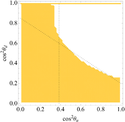
Figure 3: Constraints on θusubscript𝜃𝑢\theta_{u} and θdsubscript𝜃𝑑\theta_{d} from proper breaking of the EW symmetry and perturbativity. The figure has been obtained for tanβ=10𝛽10\tan\beta=10, m10=1.8TeVsubscript𝑚101.8TeVm_{10}=1.8\,\mathrm{TeV}, M1/2=600GeVsubscript𝑀12600GeVM_{1/2}=600\,\mathrm{GeV}, r=1𝑟1r=1. Also shown are the approximate constraints in eq. (37) (dotted lines).

The angles θusubscript𝜃𝑢\theta_{u} and θdsubscript𝜃𝑑\theta_{d} also enter the EWSB conditions through the tree level expression for the Higgs soft masses. In order for EWSB to take place for a given value of tanβ𝛽\tan\beta (and MZsubscript𝑀𝑍M_{Z}), the following two conditions have to be satisfied:

mhd2mhu2tan2βtan2β1MZ2/2(mhd2mhu2)tan2β+1tan2β1+MZ2>0.subscriptsuperscript𝑚2subscript𝑑subscriptsuperscript𝑚2subscript𝑢superscript2𝛽superscript2𝛽1subscriptsuperscript𝑀2𝑍2subscriptsuperscript𝑚2subscript𝑑subscriptsuperscript𝑚2subscript𝑢superscript2𝛽1superscript2𝛽1subscriptsuperscript𝑀2𝑍0\begin{gathered}\frac{m^{2}_{h_{d}}-m^{2}_{h_{u}}\tan^{2}\beta}{\tan^{2}\beta-1}\geq M^{2}_{Z}/2\\ (m^{2}_{h_{d}}-m^{2}_{h_{u}})\frac{\tan^{2}\beta+1}{\tan^{2}\beta-1}+M^{2}_{Z}>0\,.\end{gathered} (36)

For moderately large values of tanβ𝛽\tan\beta and in the typical fine tuned situation in which |mhu2|MZ2much-greater-thansubscriptsuperscript𝑚2subscript𝑢subscriptsuperscript𝑀2𝑍|m^{2}_{h_{u}}|\gg M^{2}_{Z}, the latter conditions become mhu20less-than-or-similar-tosubscriptsuperscript𝑚2subscript𝑢0m^{2}_{h_{u}}\lesssim 0 and mhd2mhu20greater-than-or-equivalent-tosubscriptsuperscript𝑚2subscript𝑑subscriptsuperscript𝑚2subscript𝑢0m^{2}_{h_{d}}-m^{2}_{h_{u}}\gtrsim 0. The corresponding constraints on θusubscript𝜃𝑢\theta_{u} and θdsubscript𝜃𝑑\theta_{d} can be obtained in analytical form in the limit in which eqs. (54) hold (a typical fine tuned scenario with moderately large tanβ𝛽\tan\beta and sfermions heavier than gauginos):

cos2θd+(1ρ2)cos2θu65ρ2cos2θu3/5ρ/21ρ/2.formulae-sequencegreater-than-or-equivalent-tosuperscript2subscript𝜃𝑑1𝜌2superscript2subscript𝜃𝑢65𝜌2greater-than-or-equivalent-tosuperscript2subscript𝜃𝑢35𝜌21𝜌2\cos^{2}\theta_{d}+\Big{(}1-\frac{\rho}{2}\Big{)}\cos^{2}\theta_{u}\gtrsim\frac{6}{5}-\frac{\rho}{2}\qquad\cos^{2}\theta_{u}\gtrsim\frac{3/5-\rho/2}{1-\rho/2}\,. (37)

Finally, some values of cosθusubscript𝜃𝑢\cos\theta_{u} and cosθdsubscript𝜃𝑑\cos\theta_{d} may not be allowed even if the constraints in eq. (36) hold, for example because some particle becomes tachyonic.

The constraints on θusubscript𝜃𝑢\theta_{u} and θdsubscript𝜃𝑑\theta_{d} from proper EWSB should be merged with the ones from fermion masses (eqs. (35)). The constraint θu=𝒪(1)subscript𝜃𝑢𝒪1\theta_{u}=\mathcal{O}\left(1\right) is automatically satisfied once eqs. (36) hold, while the constraint on θdsubscript𝜃𝑑\theta_{d} in eqs. (35) cuts an additional thin stripe of parameter space close to the cos2θd=1superscript2subscript𝜃𝑑1\cos^{2}\theta_{d}=1 axis. The overall constraint one gets in the cos2θusuperscript2subscript𝜃𝑢\cos^{2}\theta_{u}cos2θdsuperscript2subscript𝜃𝑑\cos^{2}\theta_{d} plane is shown (for fixed values of the other parameters) in figure 3. The allowed points with cos2θusuperscript2subscript𝜃𝑢\cos^{2}\theta_{u} near the left vertical bound (where mhu2subscriptsuperscript𝑚2subscript𝑢m^{2}_{h_{u}} changes sign) correspond to smaller |mhu2|subscriptsuperscript𝑚2subscript𝑢|m^{2}_{h_{u}}| and therefore relatively smaller fine-tuning. We see from the figure that a pure embedding of the MSSM up Higgs in the 𝟏𝟎Hsubscript10𝐻\mathbf{10}_{H} (with no component in 𝟏𝟔¯Hsubscript¯16𝐻\overline{\mathbf{16}}_{H}, cosθu=1subscript𝜃𝑢1\cos\theta_{u}=1) is allowed, while the down Higgs must have a mixed embedding, with components in both the 𝟏𝟔Hsubscript16𝐻\mathbf{16}_{H} and 𝟏𝟎Hsubscript10𝐻\mathbf{10}_{H}. A component in the 𝟏𝟔Hsubscript16𝐻\mathbf{16}_{H} is needed to obtain non vanishing down quark masses (at the tree, renormalizable level), while a component in the 𝟏𝟎Hsubscript10𝐻\mathbf{10}_{H} is necessary for a correct EWSB.

4.2 A 125 GeV Higgs
Refer to caption
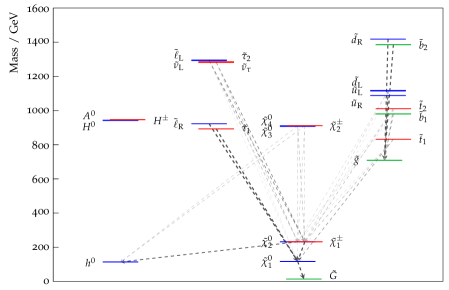
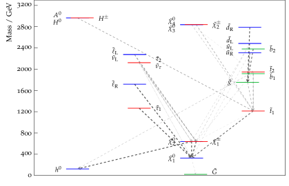
Figure 4: The SUSY spectrum of a point with a Higgs mass of 125 GeV, calculated with our modified version of the softSUSY package [6]. The decays are depicted by the dashed grey arrows, which are scaled with the respective BR calculated via SUSY-HIT [11]: only BRs greater than 0.1 are shown. The point corresponds to m10=1.5TeVsubscript𝑚101.5TeVm_{10}=1.5~{}\,\mathrm{TeV}, cosθu=0.9subscript𝜃𝑢0.9\cos\theta_{u}=0.9, cosθd=0.9subscript𝜃𝑑0.9\cos\theta_{d}=0.9, γ=16.7𝛾16.7\gamma=16.7, r=1𝑟1r=1, rD1,2=rL1,2=0.3subscriptsubscript𝑟𝐷12subscriptsubscript𝑟𝐿120.3{r_{D}}_{1,2}={r_{L}}_{1,2}=0.3, tanβ=10𝛽10\tan\beta=10, sign(μ)=+sign𝜇\text{sign}(\mu)=\mathbf{+}.

.

In standard gauge mediation it is not easy to accommodate a rather heavy Higgs boson with a mass of about 125GeV125GeV125\,\mathrm{GeV}, as indicated by the recent evidence [8, 9]. Such a mass needs in fact moderately large tanβ𝛽\tan\beta and a rather heavy SUSY scale or large trilinear couplings, see, e.g. [10]. In standard gauge mediation it is usually assumed that the messengers have only gauge interactions with the SM fields and hence the trilinear couplings are strongly suppressed at the messenger scale. RGE running does give rise to a non-negligible contribution to the A𝐴A-terms, but not large enough [12]. Sizeable trilinear terms can be generated by introducing superpotential messenger matter interactions. However, the latter potentially spoil the flavour universality of the soft terms, one of the main motivations for gauge mediation models (see however [13, 14, 15]).

Things are different in our setup. Sizeable trilinears are generated because the messengers unavoidably have Yukawa couplings to the MSSM fields, as we discussed in section 3.4. Such trilinears arise at the one loop level but they turn out to enjoy a potential enhancement by the same parameter γ𝛾\gamma enhancing gaugino masses. Moreover, because of the SO(10)𝑆𝑂10SO(10) relations between them, the flavour structure of the messenger matter couplings is dictacted by the SM Yukawas. As a consequence, they do not spoil the solution of the supersymmetric flavour problem offered by our framework. A spectrum reproducing a light Higgs of 125 GeV is shown in figure 4.

Alternatively the Higgs mass can be increased above the MSSM values in the presence of a mixing with a SM singlet chiral field S𝑆S, as in the NMSSM [16]. In MGM, such a SM singlet would have vanishing soft mass at the messenger scale, as it does not couple to SM gauge interactions. This is not necessarily the case in TGM, as the soft masses are generated by U(1)X𝑈subscript1𝑋U(1)_{X} gauge interactions. Depending on the SO(10)𝑆𝑂10SO(10) embedding of the Shuhd𝑆subscript𝑢subscript𝑑Sh_{u}h_{d} interaction lifting the Higgs mass, such a singlet could acquire a positive, vanishing, or negative soft mass. In fact, let us remind that husubscript𝑢h_{u} can be embedded into a 𝟏𝟎10\mathbf{10} or a 𝟏𝟔¯¯16\overline{\mathbf{16}}, while hdsubscript𝑑h_{d} can be embedded into a 𝟏𝟎10\mathbf{10} or a 𝟏𝟔16\mathbf{16}. We therefore have 4 possibilities for the SO(10)𝑆𝑂10SO(10) embedding of the Shuhd𝑆subscript𝑢subscript𝑑Sh_{u}h_{d} interaction: 𝟏S𝟏𝟎hu𝟏𝟎hdsubscript1𝑆subscript10subscript𝑢subscript10subscript𝑑\mathbf{1}_{S}\mathbf{10}_{h_{u}}\mathbf{10}_{h_{d}}, 𝟏𝟔¯S𝟏𝟔¯hu𝟏𝟎hdsubscript¯16𝑆subscript¯16subscript𝑢subscript10subscript𝑑\overline{\mathbf{16}}_{S}\overline{\mathbf{16}}_{h_{u}}\mathbf{10}_{h_{d}}, 𝟏𝟔S𝟏𝟎hu𝟏𝟔hdsubscript16𝑆subscript10subscript𝑢subscript16subscript𝑑\mathbf{16}_{S}\mathbf{10}_{h_{u}}\mathbf{16}_{h_{d}}, 𝟏S𝟏𝟔¯hu𝟏𝟔hdsubscript1𝑆subscript¯16subscript𝑢subscript16subscript𝑑\mathbf{1}_{S}\overline{\mathbf{16}}_{h_{u}}\mathbf{16}_{h_{d}} (where 𝟏Ssubscript1𝑆\mathbf{1}_{S} can be substituted by 𝟒𝟓Ssubscript45𝑆\mathbf{45}_{S} or 𝟓𝟒Ssubscript54𝑆\mathbf{54}_{S} without affecting our conclusions). The soft terms of the singlet S𝑆S is correspondingly given by m~S2=0,5m102,5m102,0subscriptsuperscript~𝑚2𝑆05subscriptsuperscript𝑚2105subscriptsuperscript𝑚2100\tilde{m}^{2}_{S}=0,-5m^{2}_{10},5m^{2}_{10},0. If the soft mass is negative, a vev for the S𝑆S field (and a solution for the μ𝜇\mu problem) can be induced. In the following, we will take into account the possibility of an NMSSM-like extra contribution to the Higgs mass. However, we will not enter the model building details associated to the possible presence of a NMSSM singlet in the TeV scale spectrum, leaving them to forthcoming studies.

4.3 NLSP
Refer to caption
Refer to caption
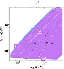
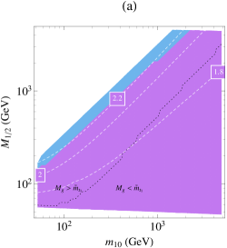
Figure 5: Nature of the NLSP in the allowed m10subscript𝑚10m_{10}M1/2subscript𝑀12M_{1/2} parameter space for tanβ=10𝛽10\tan\beta=10, cosθu=0.9subscript𝜃𝑢0.9\cos\theta_{u}=0.9, cosθd=0.9subscript𝜃𝑑0.9\cos\theta_{d}=0.9, sign(μ)=1sign𝜇1\text{sign}(\mu)=1, and r=1𝑟1r=1 (a) or r=0.2𝑟0.2r=0.2 (b). The NLSP is a neutralino in the violet region and a stau in the light blue region. The violet region corresponds to a bino like neutralino in the left panel (a) and to a wino like neutralino in the right panel (b). The regions in which the lightest coloured particle is a stop or a gluino are separated by a black dotted line. Also shown is the ratio me~L2/me~R2subscriptsuperscript𝑚2subscript~𝑒𝐿subscriptsuperscript𝑚2subscript~𝑒𝑅m^{2}_{\tilde{e}_{L}}/m^{2}_{\tilde{e}_{R}} of left and right handed squared selectron masses (white yellow lines).

In TGM models, the Lightest Supersymmetric Particle (LSP) is the gravitino. The cosmology of the model is therefore determined first of all by the nature of the Next to LSP (NLSP) which has a lifetime of hundreds of picoseconds in our benchmark points. The cosmology of such a NLSP is a interesting subject on its own and was studied before elsewhere [1, 17] so that we will not discuss it here further. The NLSP turns out to be a neutralino or the stau, depending on the region of the parameter space. Whether the lightest neutralino is bino like or wino like is essentially determined by the parameter r𝑟r, as illustrated by figure 2. When r0.3greater-than-or-equivalent-to𝑟0.3r\gtrsim 0.3, the NLSP is either a bino like neutralino or a stau, while when r0.3less-than-or-similar-to𝑟0.3r\lesssim 0.3 the NLSP is either a wino like neutralino or a stau. Figure 5 shows the part of the parameter space in which the NLSP is a neutralino (violet) or a stau (light blue). On the left panel, r=1𝑟1r=1 and the neutralino is bino like, while on the right panel r=0.2𝑟0.2r=0.2 and the neutralino is wino like. The remaining parameters are tanβ=10𝛽10\tan\beta=10, cosθu=0.9subscript𝜃𝑢0.9\cos\theta_{u}=0.9, cosθd=0.9subscript𝜃𝑑0.9\cos\theta_{d}=0.9, sign(μ)=1sign𝜇1\text{sign}(\mu)=1. The figure shows that the NLSP is a neutralino in most of the parameter space. On the other hand, a stau stripe is present in both cases. This is because the upper left boundary of the parameter space is due to the stau becoming tachyonic. A stau NLSP can therefore be obtained in a region close enough to that boundary. The regions in which the lightest coloured particle is the lightest stop or the gluino are separated by a dotted line. Finally, the ratio of left and right handed squared selectron masses is also shown (dashed white lines). As a peculiar prediction of the minimal SO(10)𝑆𝑂10SO(10) TGM scenario, that ratio is predicted to be two at the tree level. A calculable deviation from two is induced by loop corrections due to RGE running and minimal gauge mediation effects. The figure shows the prediction for the me~L2/me~R2subscriptsuperscript𝑚2subscript~𝑒𝐿subscriptsuperscript𝑚2subscript~𝑒𝑅m^{2}_{\tilde{e}_{L}}/m^{2}_{\tilde{e}_{R}} mass ratio, including the radiative correction. In the Bino NLSP case, the radiative corrections have a smaller impact (up to 10%) on the tree-level value, while in the Wino case, the impact can reach 20–30%.

In the light of the discussion above, we will consider three representative points in the parameter space in which the NLSP is a bino like neutralino, a wino like neutralino or a stau.

4.4 Three benchmark points

TGM models can provide a variety of signatures at the LHC. The nature of the NLSP and its long lifetime dictate the phenomenology. When the neutralino is the NLSP, a classical CMSSM-like phenomenology: colored sparticles are produced in the collision. The subsequent cascade generates events with missing transverse energy, jets, and possibly leptons. The decay of the NLSP to gravitino happens outside the detector.

When the NLSP is a charged particle (e.g. staus), SUSY could be found looking for heavy stable charged particles (HSCP). This kind of signature usually implies a dedicated reconstruction of the HSCP, which crosses the detector layers out of time with respect to the other particles (being slower). One then needs to connect different hits in different bunch crossings. At the same time, just looking at the collision bunch crossing (as it is done in the standard reconstruction) one typically fails to reconstruct the HSCP. The rest of the SUSY event will then look like a typical event with MET, as in the case of neutralino NLSP.

The phenomenology changes whenever the squarks and gluons are above the TeV. The squark-squark cross section becomes negligible for the luminosity collected by LHC for the first run. The main production mechanisms are gluino-squark and gluino-gluino. This implies that, despite the 3rd generation squarks being the lightest, their production is not dominant. The production of charginos and neutralinos (ewkinos) is suppressed by the coupling but enhanced by the low mass and it could become the dominant production mechanism. The detection of these events is challenging for the LHC experiments, when the ewkinos are close in mass and only soft particles are produced in the decay. The SUSY production with associated jets is then the most effective process to access these events, for instance with a monojet or a dijet analysis.

We consider three benchmark points with different NLSP, to highlight the main phenomenological implications with specific examples. Let us discuss their main features before entering the details of collider searches.

Point m10subscript𝑚10m_{10} in TeV cosθusubscript𝜃𝑢\cos\theta_{u} cosθdsubscript𝜃𝑑\cos\theta_{d} γ𝛾\gamma r𝑟r tanβ𝛽\tan\beta sign (μ)sign 𝜇\text{sign }(\mu)
Bino 1.0 0.9 0.9 15 1 10 +1
Wino 0.55 0.9 0.9 20 0.2 10 +1
Stau 0.8 0.9 0.9 35 1 35 +1
Table 3: TGM parameters for our three benchmark points with the NLSP as specified and for the point with the light Higgs mass of about 125 GeV.

4.4.1 Bino NLSP benchmark point

Refer to caption
Figure 6: The SUSY spectrum of the benchmark point with bino NLSP calculated with our modified version of the softSUSY package [6]. The decays are depicted by the dashed grey arrows, which are scaled with the respective BR calculated via SUSY-HIT [11]: only BRs greater than 0.1 are shown. The point corresponds to m10=1.0TeVsubscript𝑚101.0TeVm_{10}=1.0~{}\,\mathrm{TeV}, cosθu=0.9subscript𝜃𝑢0.9\cos\theta_{u}=0.9, cosθd=0.9subscript𝜃𝑑0.9\cos\theta_{d}=0.9, γ=15𝛾15\gamma=15, r=1𝑟1r=1, tanβ=10𝛽10\tan\beta=10, sign(μ)=+sign𝜇\text{sign}(\mu)=\mathbf{+}.

The case in which the NLSP is a bino like neutralino is the most common one if r𝑟r is not too small. As figure 5 shows, the me~L2/me~R2subscriptsuperscript𝑚2subscript~𝑒𝐿subscriptsuperscript𝑚2subscript~𝑒𝑅m^{2}_{\tilde{e}_{L}}/m^{2}_{\tilde{e}_{R}} ratio is typically within 10% of the tree-level prediction, even for a relatively light spectrum.

In the case of the benchmark point we choose, corresponding to the spectrum in figure 6, the typical final states at the LHC are characterized by a large presence of b𝑏b-enriched final states accompanied by multileptonic signals. The b𝑏b quarks and leptons largely come from the electroweak decays of the charginos and neutralinos down to the NLSP. The gaugino mass separation allows the interesting possibility that the lightest Higgs is produced in cascade decays, as the χ20χ10Hsuperscriptsubscript𝜒20superscriptsubscript𝜒10𝐻\chi_{2}^{0}\to\chi_{1}^{0}H decay is kinematically allowed, in turn characterized by the subsequent on-shell decay to b𝑏b quark pairs. Because of the large MET associated to the NLSP, which escapes detection before decaying to the gravitino, the characteristic feature of such models would be the presence of both SUSY signatures and the Higgs boson in the same event. The latter situation makes it profitable to consider such a scenario both with inclusive and exclusive dedicated searches as we shall see in the following.

4.4.2 Wino NLSP benchmark point
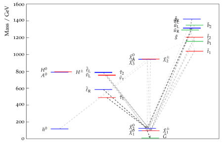
Refer to caption
Figure 7: The SUSY spectrum of the benchmark point with wino NLSP calculated with our modified version of the softSUSY package [6]. The decays are depicted by the dashed grey arrows, which are scaled with the respective BR calculated via SUSY-HIT [11]: only BRs greater than 0.1 are shown. The point corresponds to m10=550GeVsubscript𝑚10550GeVm_{10}=550~{}\,\mathrm{GeV}, cosθu=0.9subscript𝜃𝑢0.9\cos\theta_{u}=0.9, cosθd=0.9subscript𝜃𝑑0.9\cos\theta_{d}=0.9, γ=20𝛾20\gamma=20, r=0.2𝑟0.2r=0.2, tanβ=10𝛽10\tan\beta=10, sign(μ)=+sign𝜇\text{sign}(\mu)=\mathbf{+}.

The case in which the NLSP is a wino like neutralino usually leads to a heavier spectrum than obtained in the bino case. The tree-level prediction m~l2=2m~ec2subscriptsuperscript~𝑚2𝑙2subscriptsuperscript~𝑚2superscript𝑒𝑐\tilde{m}^{2}_{l}=2\tilde{m}^{2}_{e^{c}}, m~dc2=2m~q,uc2subscriptsuperscript~𝑚2superscript𝑑𝑐2subscriptsuperscript~𝑚2𝑞superscript𝑢𝑐\tilde{m}^{2}_{d^{c}}=2\tilde{m}^{2}_{q,u^{c}} gives rise to a separation between two groups of soft masses in the light families of both the slepton and squark sector. The inverted hierarchy between the two lightest gaugino masses, M2<M1subscript𝑀2subscript𝑀1M_{2}<M_{1}, makes the lightest chargino and the lightest neutralino approximately degenerate, as they have both mass M2subscript𝑀2M_{2} before EWSB. This makes the decay into the NLSP particularly soft and makes the decay χ20χ10Hsuperscriptsubscript𝜒20superscriptsubscript𝜒10𝐻\chi_{2}^{0}\to\chi_{1}^{0}H kinematically forbidden, unlike what discussed in the bino NLSP case. From this point of view, it is then comparatively more profitable to use semi- and full-leptonic channels, because of the absence of Hbb¯𝐻𝑏¯𝑏H\rightarrow b\overline{b} in the decay chain.

4.4.3 Stau NLSP benchmark point
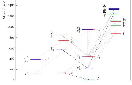
Refer to caption
Figure 8: The SUSY spectrum of the benchmark point with stau NLSP calculated with our modified version of the softSUSY package [6]. The decays are depicted by the dashed grey arrows, which are scaled with the respective BR calculated via SUSY-HIT [11]: only BRs greater than 0.1 are shown. The point corresponds to m10=800GeVsubscript𝑚10800GeVm_{10}=800~{}\,\mathrm{GeV}, cosθu=0.9subscript𝜃𝑢0.9\cos\theta_{u}=0.9, cosθd=0.9subscript𝜃𝑑0.9\cos\theta_{d}=0.9, γ=35𝛾35\gamma=35, r=1𝑟1r=1, tanβ=35𝛽35\tan\beta=35, sign(μ)=+sign𝜇\text{sign}(\mu)=\mathbf{+}.

The gaugino masses are determined by the parameter M1/2subscript𝑀12M_{1/2}, while the sfermion masses (at the tree level) are associated to m10subscript𝑚10m_{10}. For larger M1/2/m10subscript𝑀12subscript𝑚10M_{1/2}/m_{10}, one therefore expects the NLSP to be the lightest sfermion, i.e. the lightest stau. This is the case, but only in a small portion of the parameter space, as the radiative corrections to the stau mass proportional to the gaugino masses can make the stau leptons heavier than the gauginos even for largish M1/2/m10subscript𝑀12subscript𝑚10M_{1/2}/m_{10}. The stau NLSP region in figure 5 are close to the upper-left border of the parameter space, which is associated to the stau becoming more than light: tachyonic. In the regions of parameter space characterized by a stau NLSP the tree level and the M1/2subscript𝑀12M_{1/2}-driven radiative contributions to coloured sfermion masses are comparable. It is therefore necessary to include the latter contribution in order to test the TGM prediction for the sfermion mass ratios. The stau is not expected to decay to the gravitino in the detector. One can then use searches for heavy charged stable particles, on top of inclusive ones.

5 TGM phenomenology at the LHC

The search for SUSY with MET at the LHC has made remarkable progresses with respect to the previous experiments. The favourable beam energy and the large luminosity collected are the basic ingredients that determined this improvement. On the other hand, many progresses have been made also on the analysis technique, with new ideas introduced to suppress the background and increase the signal sensitivity. The ATLAS and CMS experiments have collected so far 5similar-toabsent5\sim~{}5 fb-1 at 7 TeV and are expected to collect 20similar-toabsent20\sim~{}20 fb-1 at 8 TeV. The current limits are pushing the masses of the coloured superpartners above the 1 TeV threshold for generic MSSM models [18, 19], while lower masses are allowed for stop and sbottom in the case of models with large mass splitting among the third family and the others [20, 21]. So far, the possibility of light charginos and neutralinos has been tested only through multi lepton final states [22, 23], which suffer from the suppression coming from Z𝑍Z\to\ell\ell and Wν𝑊𝜈W\to\ell\nu branching ratios. The increase in the center of mass energy will be beneficial to push the mass limits on squarks and gluino above the TeV scale, while the search for light EW gauginos will be pushed by the larger collected luminosity.

In this scenario, a possible hint of new physics could emerge by the end of 2012, but even in this situation the mission would be far from being accomplished. The search for SUSY would be completed by the characterization of a possible excess in terms of a specific SUSY model, to possibly underline the nature of the SUSY breaking mechanism and of its mediation. Accomplishing this goal, sometimes referred to as the inverse LHC problem [24], would imply the use of kinematic variables sensitive to the mass of the produced particles in as many final states as possible.

The TGM class of models offers a rich phenomenology at the LHC, challenging the experiments on several fronts at the same time (e.g. high mass searches, compressed gaugino spectra, \dots) and allowing several many interesting possibilities, such as Higgs production in SUSY cascades. In this respect, TGM is an interesting playground on which the performances of different searches (e.g. hadronic vs. leptonic searches) could be compared, and, on top of that, it comes with a specific prediction on the ratio of sfermion masses, which should be tested by experiments in case an excess is found.

A full review of all the analyses presented by ATLAS and CMS and their implications on TGM goes beyond the scope of this paper. Instead, we consider only the CMS razor analysis [25, 21], which offers a set of interesting features:

  1. 1.

    It considers simultaenously six final states (1μ1e1𝜇1𝑒1\mu 1e, 2μ2𝜇2\mu, 2e2𝑒2e, 1μ1𝜇1\mu, 1e1𝑒1e, and hadronic) providing in one goal the combination of six different analyses.

  2. 2.

    It gives a competitive limit on all the signatures it is sensitive to, giving a reasonable estimate of the current constraints from the full LHC SUSY program.

  3. 3.

    Besides being sensitive to a signal, it also offers some information on the underlying SUSY spectrum, in case a signal is seen.

This last feature is particularly interesting for TGM models. From the general discussion in appendix C we see that as far as our spectrum is characterized by two well defined mass scales, namely corresponding to q~,u~c~𝑞superscript~𝑢𝑐\tilde{q},\tilde{u}^{c} and d~csuperscript~𝑑𝑐\tilde{d}^{c} squarks, the distribution of the MRsubscript𝑀𝑅M_{R} variable will identify the latter as two different peaks of definite mass. More specifically such peaks will occur for those values of MΔsubscript𝑀ΔM_{\Delta}, see eq. (57), corresponding to the decays of the squarks towards the NLSP. The peculiar phenomenological prediction of minimal unified TGM, the ratio in equation (7) would then be translated to a ratio between the position of the two peaks in the distribution of MRsubscript𝑀𝑅M_{R} given by

MΔdc,lMΔq,uc,ec=2(1+mNLSP22m102+).superscriptsubscript𝑀Δsuperscript𝑑𝑐𝑙superscriptsubscript𝑀Δ𝑞superscript𝑢𝑐superscript𝑒𝑐21subscriptsuperscript𝑚2NLSP2subscriptsuperscript𝑚210\frac{M_{\Delta}^{d^{c},l}}{M_{\Delta}^{q,u^{c},e^{c}}}=\sqrt{2}\left(1+\frac{m^{2}_{\rm{NLSP}}}{2{m}^{2}_{10}}+\dots\right)\,. (38)

Unfortunately the situation just depicted is too simplistic as many different effects tend to broaden the MRsubscript𝑀𝑅M_{R} distribution, causing a partial or total overlap of the different peaks. Anyway, with high luminosity and sufficient separation (30%greater-than-or-equivalent-toabsentpercent30\gtrsim 30\% of the peak position) one could distinguish the peaks even in presence of detector effects.

5.1 Analysis of the benchmark points

We start by computing the SUSY spectrum evolving the parameters of eqs. (3) and (4) with the RGEs described in appendix B down to low energies using a modified version of the softSUSY package [6]; knowing the spectrum we calculate the branching ratios via SUSY-HIT [11]. Then we generate a sample of SUSY events at the center of mass energy of 7 TeV using PYTHIA8 [27]. We cluster jets from the stable particles in the event, ignoring neutrinos and the NLSP, with the anti-Kt jet algorithm [28] as implemented in FASTJET [29, 30]. The energy of the generator level jets is then modified in order to take into account the detector resolution of the CMS detector [31]. The resolution is modeled according to a Gaussian response function both for the jet transverse momenta and the missing transverse energy (MET).

Our emulation of the CMS razor analysis follows the guideline provided by the CMS collaboration [26]. We emulate the performances of the CMS detector according to the provided instructions before applying the analysis selection. We use the events surviving the selection to build the 2D R2superscript𝑅2R^{2} vs MRsubscript𝑀𝑅M_{R} distributions for the six exclusive boxes, which are used to derive a limit on the cross section for a given SUSY model. The limit is computed running the code provided by the CMS collaboration, which combines the six exclusive boxes and incorporate the uncertainty on the signal and the background distributions. It is interesting to compare the distribution of MRsubscript𝑀𝑅M_{R} and R2superscript𝑅2R^{2} in different boxes. In case of an observation, the prominence of the different MRsubscript𝑀𝑅M_{R} peaks in different boxes could be used to understand which sparticles could have been produced in the collision or in the decay.


Different boxes are differently important for different models (see Fig. 9). For instance, the wino benchmark model is characterized by the production of ewkinos, which are too close in mass for the model to be observable. In this case, SUSY production is accessible only through the associated jet production, which explains why the events fraction in the hadronic box is very close to one. For the other models the event fraction in the hadronic box goes down to 80%similar-toabsentpercent80\sim 80\%, while 510%similar-toabsent5percent10\sim 5-10\% of the events fill the single-lepton and the MuMu boxes. Given the larger background contamination in the Had box, a larger yield does not necessarily correspond to a better signal-to-background discrimination.
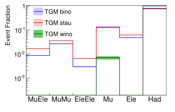
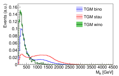
Refer to caption
Figure 9: Relative fraction of signal events in the six razor boxes, for the three considered benchmark models.

Refer to caption
Refer to caption
Refer to caption
Refer to caption
Refer to caption
Refer to caption
Figure 10: MRsubscript𝑀𝑅M_{R} (left) and R2superscript𝑅2R^{2} (right) distributions for a set of TGM benchmark points, as obtained for the CMS razor hadronic (top), leptonic (center), and dileptonic (bottom) boxes.

We show in figure 10 the MRsubscript𝑀𝑅M_{R} and R2superscript𝑅2R^{2} projections for the hadronic, leptonic, and semileptonic boxes in the benchmark points under analysis. One could notice that the different decay chains produce different distributions, even within one model. The presence of two competitive decay chains in one model generates a multimodal distribution, each local maximum corresponding to a different mass split between the produced sparticle and the NLSP. One should notice that we further assume the stable staus to be too slow to be detected with the ordinary event reconstruction555Recently, it was also pointed out that these particles could receive a boost if produced in the cascade decay of heavier particles. In this case they should be detected as ordinary muons, with no missing energy in the event. In this sense, any conclusion we obtain neglecting this effect overestimates the sensitivity of the razor analysis to these models, since a misidentification of the stau as a muon would reduce the value of R2superscript𝑅2R^{2} and consequently the efficiency of the analysis..

The MRsubscript𝑀𝑅M_{R} distribution is characterized by two peaks. The broad peak around 1 TeV in the hadronic box for the stau and the bino models is the overlap of the competing gluino-gluino and squark-gluino production mechanisms. Due to the resolution in MRsubscript𝑀𝑅M_{R} and the small mass differences between the squarks and the gluino, it is not possible to resolve the different peaks. This peak is also present in the leptonic boxes, the lepton being produced in the cascade decays of the squarks, typically from W𝑊W and Z𝑍Z bosons coming from ewkinos.

The second peak at low MRsubscript𝑀𝑅M_{R} has a different origin. The events around this peak originate from the production of charginos and neutralinos. Being very close in mass, these particles tend to produce soft objects (jets or leptons) when decaying to the NLSP. These events are in general rejected by the event selection, which requires two jets with a transverse momentum of at least 60 GeV, unless the charginos and neutralinos are produced in association with at least two jets coming from initial or final state radiation. In this case, the visible jet and the invisible massive particles do not originate from the decay of a heavy sparticle, as the razor construction assumes. These events correspond to a non resonant production and no peak in MRsubscript𝑀𝑅M_{R} is expected. If the jet pTsubscript𝑝𝑇p_{T} requirement was lower, one would see a falling distribution for MRsubscript𝑀𝑅M_{R}. On the other hand, only events with two energetic jets enter the distribution. These events have an intrinsic requirement on the minimum visible energy of the event, which (due to the correlation between MRsubscript𝑀𝑅M_{R} and the visible energy) scalps the MRsubscript𝑀𝑅M_{R} distribution at low values, producing what looks like a peak at low MRsubscript𝑀𝑅M_{R}. Unlike the case of genuine kinematic peaks, the position of this peak is not related to the SUSY spectrum, being a model-independent artifact of the event selection. The abundance of these events is maximal for hadronic events and reduced for one-lepton events, while it become subdominant for two-lepton events. In the case of the wino benchmark point the split in mass between the chargino and the neutralino is so small that the leptons are undetected in the majority of the cases. As a consequence, almost all the events fall in the hadronic box. The relative importance of the two contributions in different boxes could give an insight of the relative cross sections for the two classes of process, which eventually could allow to constrain the mass scale associated to the produced particles.

Following the instructions given by CMS [26] we compute the excluded cross section for each benchmark model and compare it to the next to leading order (NLO) value, obtained running PROSPINO [32]. In the case of the stau benchmark point one would need a more detailed detector simulation to correctly take into account the fraction of events in which the two staus actually contribute to the missing transverse energy in the event. If this fraction is small, the limit would be much weaker than what is quoted in Table 4.

Model NLO SUSY Had-box excluded Total excluded
cross section [pb] cross section [pb] cross section [pb]
TGM bino 0.027 0.024 0.019
TGM wino 12.02 4.3 3.5
TGM stau 0.002 0.010 0.008
Table 4: Theoretical NLO SUSY cross section for the three benchmark points obtained from PROSPINO [32] compared to the excluded cross section (at 95% probability) estimated with our implementation of the razor analysis by the CMS collaboration, according to the procedure given by the CMS collaboration [26]. Both the limit from the Hadronic box and the combined limit are shown.

The largest sensitivity comes from the hadronic box, which collects the majority of the events originating from the production of colored sparticles. The improvement due to the leptonic boxes is marginal for the considered benchmark models. The stau and the bino models are not excluded. But the observed limit is not far from the model cross section, such that the analysis of the 8 TeV data could already rule them out. The wino point is excluded, despite being the most challenging. This proves that the cross section production for ewkinos lighter than 200 GeV is already probed by the 7 TeV LHC data, the cross section being above 1 pb. Additional sensitivity could be provided by dedicated searches for directly-produced charginos and neutralinos. The exclusion reach by the ATLAS [33] and CMS [34] multilepton analyses, obtained considering the full 8 TeV statistics, is not good enough to cover the benchmark models we considered. This is mainly due to the large chargino and neutralino masses and the corresponding suppression of the production cross section. These benchmark models could be probed with the next LHC run, thanks to the larger production cross section and the larger expected statistics.
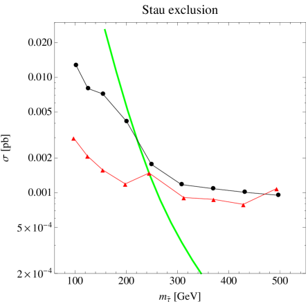

Refer to caption
Figure 11: In order to set some limits on the NLSP stau mass we calculated the predicted theoretical cross section and then compared the latter with the observed 95% CL upper limit [35]. The black line represents the experimental bound on the cross section taking into account only the selection based on the tracker, while the red line is based also on the time of flight (TOF). The green line gives the theoretical direct production cross sections for staus on which we added the subleading contribution of the indirect stau production owed to the squark and gluino channels, all of these contribution computed through PROSPINO [32]. All in all we can give a mass bound for the stau of 220 ÷\div 250 GeV.

Finally, in the case in which the NLSP is the stau some bounds on its mass can be set from the searches on the heavy charged stable particles, as anticipated in section 4.4.3: the stau, indeed, decays to the gravitino outside the detector. Such limits in the TGM framework are in general less restrictive than those in MGM since the additive tree level contribution to stau soft mass term accounts for a comparably smaller production cross section. As shown in figure 11, the recent experimental results allows a TGM stau mass larger than 220 ÷\div 250 GeV. In that plot, we have varied m10subscript𝑚10m_{10} from 450 to 1250 GeV and fixed the other parameters at the values of the stau benchmark point.

6 Summary and conclusions

We studied the LHC phenomenology of a minimal unified realization of Tree-level Gauge Mediation, in particular the possibility to test its peculiar prediction for the sfermion mass ratios. We did this in three steps.

First, we provided a detailed definition of the Lagrangian of the model and of the relevant parameters, taking into account the possible deviations from SO(10)𝑆𝑂10SO(10) relations due to the contributions of the non-renormalizable operators necessary to fix the GUT prediction for the light fermion mass ratios.

Then we discussed the precise determination of the low energy spectrum in terms of the above parameters. In particular, we provided analytical formulas for the RGE running and a numerical implementation in softSUSY. The possible deviations from GUT relations turn out not to affect the tree-level predictions for the sfermion mass ratios. However, we pointed out that they can give rise to largely non-universal gaugino masses without any conflict with the unification of gauge couplings. The non-universality arises from the flavour structure of the messenger interactions. Even in the limit in which the SO(10)𝑆𝑂10SO(10) breaking effects are small and only significantly affect the small Yukawa couplings of the first families, the effect on gaugino masses can be sizeable. This is because gaugino masses are equally sensitive to the ratio of the larger third family Yukawa couplings and to the ratio of the smaller first family couplings, more likely to be affected by 𝒪(1)𝒪1\mathcal{O}\left(1\right) effects. As a consequence of the possible non-universality of gaugino masses, the Wino can be lighter than the Bino. Still, gaugino masses satisfy a sum rule, eq. (12), which can be considered as another smoking gun of minimal unified TGM.

Another important aspect related to the determination of the TeV-scale spectrum has to do with A𝐴A-terms. Usually in gauge mediation no A𝐴A-terms are generated at the one-loop level at the messenger scale. This is not the case here. In fact, the MSSM fields and the minimal gauge mediation messengers lie in the same SO(10)𝑆𝑂10SO(10) multiplets, so that the messenger-messenger-Z𝑍Z coupling generating gaugino masses are accompanied by matter-messenger-Z𝑍Z couplings generating non-vanishing A𝐴A-terms at the messenger scale. The size of the A𝐴A-terms depends on whether the heavier of the three families of messengers is significantly lighter than the GUT scale or not. The latter case, corresponding to third family Yukawas of order one in the full SO(10)𝑆𝑂10SO(10) theory, gives rise to larger A𝐴A-terms but is more model-dependent, as it depends on unknown details of the full SO(10)𝑆𝑂10SO(10) theory. In turn, the possibility of sizeable A𝐴A-terms allows to account for a 125GeV125GeV125\,\mathrm{GeV} light Higgs for sfermion masses within the LHC reach. On the other hand, the Higgs mass can be raised above the MSSM prediction with a suitable implementation of the NMSSM setup. Another interesting property of the A𝐴A-terms in TGM is that only the third family A𝐴A-terms are non negligible, as the first and second family are suppressed by powers of small Yukawa couplings. This solves the supersymmetric CP problem.

Different possible types of spectra can be obtained, in particular as far as the NLSP is concerned. In TGM models, the Lightest Supersymmetric Particle is the gravitino. The NLSP turns out to be a bino-like neutralino, a wino-like neutralino, or a stau. The possibility that the lightest neutralino is wino like is opened by the possible non-universality of gaugino masses. We have therefore considered three benchmark points representative of each of those possibilities.

Finally, we studied the LHC signals associated to each benchmark point, considering in particular the possibility to test the sfermion mass ratio prediction. TGM turns out to be an interesting playground on which the performances of different searches can be compared. From this point of view we found that the razor inclusive analysis by CMS was an ideal tool.

For each benchmark point, we computed the SUSY spectrum by running the parameters of the model from the GUT to the TeV scale using a modified version of the softSUSY package. We evaluated the possible signatures at the LHC applying the selection of the CMS Razor analysis, discussing the interesting interplay between the different production processes and decay chains in the different boxes in which the Razor search is defined. We also studied other interesting features of the TGM benchmark models, as for instance the long-living staus, the compressed chargino-neutralino spectrum and the large mass difference between the colored particles and the rest of the spectrum. The TGM class of models can accomodate the lack of a SUSY signal so far and the possibility of observing one with the 8 TeV data, or with the first data collected at higher energy at the LHC restart.

Acknowledgments

The work of A.R. and M.S. was supported by the ERC Advanced Grant no. 267985 “DaMESyFla”, by the EU Marie Curie ITN “UNILHC” (PITN-GA-2009-237920) and the European Union FP7 ITN invisibles (Marie Curie Actions, PITN- GA-201-289442). Part of this work was done at the Galileo Galilei Institute for Theoretical Physics, which we thank for the kind hospitality and support.

Appendix A Flavour structure of the superpotential

In this appendix, we discuss the expectations for the size of the parameters cDi,Lisubscript𝑐subscript𝐷𝑖subscript𝐿𝑖c_{D_{i},L_{i}}. As we have seen in section 3.2, the breaking of SO(10)𝑆𝑂10SO(10) and SUSY must involve spinorial representations. In particular, the 𝟏𝟔16\mathbf{16}, 𝟏𝟔¯¯16\overline{\mathbf{16}} fields acquire a vev M𝑀M in the scalar, SM singlet component and 𝟏𝟔superscript16\mathbf{16}^{\prime}, 𝟏𝟔¯superscript¯16\overline{\mathbf{16}}^{\prime} acquire a vev in the F𝐹F-term SM singlet component. As in section 3.2, we will actually assume for simplicity that only 𝟏𝟔superscript16\mathbf{16}^{\prime} gets an F𝐹F-term and we further assume that the 𝟏𝟔16\mathbf{16} and 𝟏𝟔superscript16\mathbf{16}^{\prime} are the only spinorial representations coupling to matter bilinears. For convenience we remind the form of the most general R-parity invariant superpotential bilinear in the matter fields 𝟏𝟔i+𝟏𝟎isubscript16𝑖subscript10𝑖\mathbf{16}_{i}+\mathbf{10}_{i}, eq. (14):

W2=hij𝟏𝟔i𝟏𝟎j𝟏𝟔+hij𝟏𝟔i𝟏𝟎j𝟏𝟔+yij2𝟏𝟔i𝟏𝟔j𝟏𝟎+W2NR.subscript𝑊2subscript𝑖𝑗subscript16𝑖subscript10𝑗16subscriptsuperscript𝑖𝑗subscript16𝑖subscript10𝑗superscript16subscript𝑦𝑖𝑗2subscript16𝑖subscript16𝑗10superscriptsubscript𝑊2NRW_{2}=h_{ij}\mathbf{16}_{i}\mathbf{10}_{j}\mathbf{16}+h^{\prime}_{ij}\mathbf{16}_{i}\mathbf{10}_{j}\mathbf{16}^{\prime}+\frac{y_{ij}}{2}\mathbf{16}_{i}\mathbf{16}_{j}\mathbf{10}+W_{2}^{\text{NR}}. (39)

In the previous equation, a mass term μij𝟏𝟎i𝟏𝟎jsubscript𝜇𝑖𝑗subscript10𝑖subscript10𝑗\mu_{ij}\mathbf{10}_{i}\mathbf{10}_{j} has been assumed to be absent to obtain a “pure” embedding of the SM fields in SO(10)𝑆𝑂10SO(10) representations and to avoid reintroducing the flavour problem [2]. The (model-dependent) non-renormalizable part is not specified but it is supposed to bring the fermion mass ratios to the phenomenologically correct values.

In order to identify the light Yukawa couplings we need to specify better the embedding of the light Higgs fields, deepening the discussion in section 3.1. The light hdsubscript𝑑h_{d} can be contained in the doublet component of the 𝟏𝟔16\mathbf{16}, hd16subscriptsuperscript16𝑑h^{16}_{d}, in the doublet of the 𝟏𝟔superscript16\mathbf{16}^{\prime}, hd16subscriptsuperscriptsuperscript16𝑑h^{16^{\prime}}_{d} or in a 𝟏𝟎10\mathbf{10}, with the size of the total component in spinorial representations given by sinθdsubscript𝜃𝑑\sin\theta_{d}. The field hdsubscript𝑑h_{d} could be in principle also be embedded in a spinorial representation different from 𝟏𝟔16\mathbf{16} and 𝟏𝟔superscript16\mathbf{16}^{\prime} and not coupling to the matter bilinears, but we assume that this is not the case. We can use an angle α𝛼\alpha to measure how hdsubscript𝑑h_{d} is shared by the two spinorial representations:

hd16=sinθdcosαhd+,hd16=sinθdsinαhd+.formulae-sequencesubscriptsuperscript16𝑑subscript𝜃𝑑𝛼subscript𝑑subscriptsuperscriptsuperscript16𝑑subscript𝜃𝑑𝛼subscript𝑑h^{16}_{d}=\sin\theta_{d}\cos\alpha\,h_{d}+\text{\ldots}\,,\quad h^{16^{\prime}}_{d}=\sin\theta_{d}\sin\alpha\,h_{d}+\text{\ldots}\,. (40)

From eqs. (39) and (40) we can recover the SM Yukawa couplings λU,D,Esubscript𝜆𝑈𝐷𝐸\lambda_{U,D,E} and λ^D,Esubscript^𝜆𝐷𝐸\hat{\lambda}_{D,E} in eq. (3) as follows:

λUsubscript𝜆𝑈\displaystyle\lambda_{U} =cosθuy+λUNR,absentsubscript𝜃𝑢𝑦subscriptsuperscript𝜆NR𝑈\displaystyle=\cos\theta_{u}\,y+\lambda^{\text{NR}}_{U}\;, (41)
λEsubscript𝜆𝐸\displaystyle\lambda_{E} =sinθd(cosαh+sinαh)+λENR,absentsubscript𝜃𝑑𝛼𝛼superscriptsuperscriptsubscript𝜆𝐸NR\displaystyle=\sin\theta_{d}(\cos\alpha h+\sin\alpha h^{\prime})+\lambda_{E}^{\text{NR}}\;, λDsubscript𝜆𝐷\displaystyle\lambda_{D} =sinθd(cosαh+sinαh)+λDNR,absentsubscript𝜃𝑑𝛼𝛼superscriptsuperscriptsubscript𝜆𝐷NR\displaystyle=\sin\theta_{d}(\cos\alpha h+\sin\alpha h^{\prime})+\lambda_{D}^{\text{NR}}\;,
λ^Esubscript^𝜆𝐸\displaystyle\hat{\lambda}_{E} =cosθdy+λ^ENR,absentsubscript𝜃𝑑𝑦superscriptsubscript^𝜆𝐸NR\displaystyle=\cos\theta_{d}\,y+\hat{\lambda}_{E}^{\text{NR}}\;, λ^Dsubscript^𝜆𝐷\displaystyle\hat{\lambda}_{D} =cosθdy+λ^DNR,absentsubscript𝜃𝑑𝑦superscriptsubscript^𝜆𝐷NR\displaystyle=\cos\theta_{d}\,y+\hat{\lambda}_{D}^{\text{NR}}\;,

where the superscript ”NR” denotes a correction vanishing in the limit W2NR0subscriptsuperscript𝑊NR20W^{\text{NR}}_{2}\to 0.

From eqs. (41) one can see that the simplest possible relation between the parameters hD,Lsubscript𝐷𝐿h_{D,L} and the MSSM Yukawas is obtained when hdsubscript𝑑h_{d} is entirely in the 𝟏𝟔16\mathbf{16} and the non-renormalizable contributions are negligible, in which case we obtain eq. (17). In order to account for the general case, we have introduced new parameters cDi,Lisubscript𝑐subscript𝐷𝑖subscript𝐿𝑖c_{D_{i},L_{i}} defined by

hDisubscriptsubscript𝐷𝑖\displaystyle{h_{D}}_{i} =cDiλDi/sinθd,absentsubscriptsubscript𝑐𝐷𝑖subscriptsubscript𝜆𝐷𝑖subscript𝜃𝑑\displaystyle={c_{D}}_{i}{\lambda_{D}}_{i}/\sin\theta_{d}\;, hLisubscriptsubscript𝐿𝑖\displaystyle\qquad\qquad{h_{L}}_{i} =cLiλLi/sinθd,absentsubscriptsubscript𝑐𝐿𝑖subscriptsubscript𝜆𝐿𝑖subscript𝜃𝑑\displaystyle={c_{L}}_{i}{\lambda_{L}}_{i}/\sin\theta_{d}\;, (42)

The cDi,Lisubscript𝑐subscript𝐷𝑖subscript𝐿𝑖c_{D_{i},L_{i}} coefficients can be written in terms of the parameters in eqs. eq. (41) as follows:

cLi=1cosα+sinαγLi+(cLi)NR,cDi=1cosα+sinαγDi+(cDi)NR.formulae-sequencesubscript𝑐subscript𝐿𝑖1𝛼𝛼subscriptsubscript𝛾𝐿𝑖subscriptsubscript𝑐subscript𝐿𝑖NRsubscript𝑐subscript𝐷𝑖1𝛼𝛼subscriptsubscript𝛾𝐷𝑖subscriptsubscript𝑐subscript𝐷𝑖NR\displaystyle c_{L_{i}}=\frac{1}{\cos\alpha+\sin\alpha\,{\gamma_{L}}_{i}}+(c_{L_{i}})_{\text{NR}},\qquad c_{D_{i}}=\frac{1}{\cos\alpha+\sin\alpha\,{\gamma_{D}}_{i}}+(c_{D_{i}})_{\text{NR}}. (43)

The equations above allow to set an appropriate range for these coefficients. In the limit in which hdsubscript𝑑h_{d} lies in the 𝟏𝟔16\mathbf{16} only (α=0𝛼0\alpha=0), cDi,Li=1subscript𝑐subscript𝐷𝑖subscript𝐿𝑖1c_{D_{i},L_{i}}=1 at the renormalizable level. In the limit in which hdsubscript𝑑h_{d} lies in the 𝟏𝟔superscript16\mathbf{16^{\prime}} only (α=π/2𝛼𝜋2\alpha=\pi/2), on the other hand, the parameters cDi,Lisubscript𝑐subscript𝐷𝑖subscript𝐿𝑖c_{D_{i},L_{i}} can be smaller, especially if the parameters γD,Lsubscript𝛾𝐷𝐿\gamma_{D,L} in (19) enhance gaugino masses.

Appendix B One-loop RGEs

In this section we shall present the RGEs for the full theory below the GUT scale [36]. In all of the following equations we will use the common definition tlnμ𝑡𝜇t\equiv\ln\mu where μ𝜇\mu is the renormalization scale.

B.1 Gauge couplings

The RGEs for the gauge couplings are

(4π)2dgadt=β(1)ga,superscript4𝜋2dsubscript𝑔𝑎d𝑡superscript𝛽1subscript𝑔𝑎(4\pi)^{2}\frac{\text{d}g_{a}}{\text{d}t}=\beta^{(1)}{g_{a}}\,, (44)

where

β(1)ga=ga3RBa(R)superscript𝛽1subscript𝑔𝑎superscriptsubscript𝑔𝑎3subscript𝑅subscript𝐵𝑎𝑅\beta^{(1)}{g_{a}}=g_{a}^{3}\sum_{R}B_{a}(R) (45)

and

B3subscript𝐵3\displaystyle B_{3} =RB3(R)=3+NDc+ND2,absentsubscript𝑅subscript𝐵3𝑅3subscript𝑁superscript𝐷𝑐subscript𝑁𝐷2\displaystyle=\sum_{R}B_{3}(R)=-3+\frac{N_{D^{c}}+N_{D}}{2}\,, (46a)
B2subscript𝐵2\displaystyle B_{2} =RB2(R)=1+NL+NLc2,absentsubscript𝑅subscript𝐵2𝑅1subscript𝑁𝐿subscript𝑁superscript𝐿𝑐2\displaystyle=\sum_{R}B_{2}(R)=1+\frac{N_{L}+N_{L^{c}}}{2}\,, (46b)
B1subscript𝐵1\displaystyle B_{1} =RB1(R)=335+35(13NDc+13ND+12NL+12NLc),absentsubscript𝑅subscript𝐵1𝑅3353513subscript𝑁superscript𝐷𝑐13subscript𝑁𝐷12subscript𝑁𝐿12subscript𝑁superscript𝐿𝑐\displaystyle=\sum_{R}B_{1}(R)=\frac{33}{5}+\frac{3}{5}\Bigl{(}\frac{1}{3}N_{D^{c}}+\frac{1}{3}N_{D}+\frac{1}{2}N_{L}+\frac{1}{2}N_{L^{c}}\Bigr{)}\,, (46c)

where NDcsubscript𝑁superscript𝐷𝑐N_{D^{c}} is the number of Dcsuperscript𝐷𝑐D^{c} fields and similar for the other N𝑁N.

B.2 Gaugino masses

In terms of the results obtained for the gauge couplings one has

(4π)2dMadt=2ga2BaMa.superscript4𝜋2dsubscript𝑀𝑎d𝑡2superscriptsubscript𝑔𝑎2subscript𝐵𝑎subscript𝑀𝑎(4\pi)^{2}\frac{\text{d}M_{a}}{\text{d}t}=2g_{a}^{2}B_{a}M_{a}\,. (47)

B.3 Yukawa couplings

In the following equations, the integration of the heavy chiral messengers at their mass scale is taken into account by setting to zero the corresponding entries of the Yukawa matrices. We note that the part proportional to the gauge coupling does not depend on the number of flavours that are switched on since it is directly related to the specific λ𝜆\lambda parameter under study. Incidentally we note that if some of the flavours are frozen out this will also act on the meaning of the various traces appearing in the equations.

(4π)2dλUdtsuperscript4𝜋2dsubscript𝜆𝑈d𝑡\displaystyle(4\pi)^{2}\frac{\text{d}\lambda_{U}}{\text{d}t} =λU[Tr(3λUλU)+3λUλU+λDλD+λ^Dλ^D163g323g221315g12]absentsubscript𝜆𝑈delimited-[]Tr3superscriptsubscript𝜆𝑈subscript𝜆𝑈3superscriptsubscript𝜆𝑈subscript𝜆𝑈superscriptsubscript𝜆𝐷subscript𝜆𝐷superscriptsubscript^𝜆𝐷subscript^𝜆𝐷163superscriptsubscript𝑔323superscriptsubscript𝑔221315superscriptsubscript𝑔12\displaystyle=\lambda_{U}\Bigl{[}\operatorname{Tr}(3\lambda_{U}^{\dagger}\lambda_{U})+3\lambda_{U}^{\dagger}\lambda_{U}+\lambda_{D}^{\dagger}\lambda_{D}+{\hat{\lambda}_{D}}^{\dagger}\hat{\lambda}_{D}-\frac{16}{3}g_{3}^{2}-3g_{2}^{2}-\frac{13}{15}g_{1}^{2}\Bigr{]} (48a)
(4π)2dλDdtsuperscript4𝜋2dsubscript𝜆𝐷d𝑡\displaystyle(4\pi)^{2}\frac{\text{d}\lambda_{D}}{\text{d}t} =λD[Tr(3λDλD+3λ^Dλ^D+λEλE+λ^Eλ^E)+3λDλD+3λ^Dλ^D+λUλU]absentsubscript𝜆𝐷delimited-[]Tr3superscriptsubscript𝜆𝐷subscript𝜆𝐷3superscriptsubscript^𝜆𝐷subscript^𝜆𝐷superscriptsubscript𝜆𝐸subscript𝜆𝐸superscriptsubscript^𝜆𝐸subscript^𝜆𝐸3superscriptsubscript𝜆𝐷subscript𝜆𝐷3superscriptsubscript^𝜆𝐷subscript^𝜆𝐷superscriptsubscript𝜆𝑈subscript𝜆𝑈\displaystyle=\lambda_{D}\Bigl{[}\operatorname{Tr}(3\lambda_{D}^{\dagger}\lambda_{D}+3{\hat{\lambda}_{D}}^{\dagger}\hat{\lambda}_{D}+\lambda_{E}^{\dagger}\lambda_{E}+{\hat{\lambda}_{E}}^{\dagger}\hat{\lambda}_{E})+3\lambda_{D}^{\dagger}\lambda_{D}+3{\hat{\lambda}_{D}}^{\dagger}\hat{\lambda}_{D}+\lambda_{U}^{\dagger}\lambda_{U}\Bigr{]}
λD[163g32+3g22+715g12]subscript𝜆𝐷delimited-[]163superscriptsubscript𝑔323superscriptsubscript𝑔22715superscriptsubscript𝑔12\displaystyle{}\quad{}-\lambda_{D}\Bigl{[}\frac{16}{3}g_{3}^{2}+3g_{2}^{2}+\frac{7}{15}g_{1}^{2}\Bigr{]} (48b)
(4π2)dλEdt4superscript𝜋2dsubscript𝜆𝐸d𝑡\displaystyle(4\pi^{2})\frac{\text{d}\lambda_{E}}{\text{d}t} =[Tr(3λDλD+3λ^Dλ^D+λEλE+λ^Eλ^E)+3λEλE+3λ^Eλ^E]λEabsentdelimited-[]Tr3superscriptsubscript𝜆𝐷subscript𝜆𝐷3superscriptsubscript^𝜆𝐷subscript^𝜆𝐷superscriptsubscript𝜆𝐸subscript𝜆𝐸superscriptsubscript^𝜆𝐸subscript^𝜆𝐸3subscript𝜆𝐸superscriptsubscript𝜆𝐸3subscript^𝜆𝐸superscriptsubscript^𝜆𝐸subscript𝜆𝐸\displaystyle=\Bigl{[}\operatorname{Tr}(3\lambda_{D}^{\dagger}\lambda_{D}+3{\hat{\lambda}_{D}}^{\dagger}\hat{\lambda}_{D}+\lambda_{E}^{\dagger}\lambda_{E}+{\hat{\lambda}_{E}}^{\dagger}\hat{\lambda}_{E})+3\lambda_{E}\lambda_{E}^{\dagger}+3{\hat{\lambda}_{E}}\hat{\lambda}_{E}^{\dagger}\Bigr{]}\lambda_{E}
[3g22+95g12]λEdelimited-[]3superscriptsubscript𝑔2295superscriptsubscript𝑔12subscript𝜆𝐸\displaystyle{}\quad{}-\Bigl{[}3g_{2}^{2}+\frac{9}{5}g_{1}^{2}\Bigr{]}\lambda_{E} (48c)
(4π2)dλ^Ddt4superscript𝜋2dsubscript^𝜆𝐷d𝑡\displaystyle(4\pi^{2})\frac{\text{d}\hat{\lambda}_{D}}{\text{d}t} =λ^D[Tr(3λDλD+3λ^Dλ^D+λEλE+λ^Eλ^E)+3λ^Dλ^D+3λDλD+λUλU]absentsubscript^𝜆𝐷delimited-[]Tr3superscriptsubscript𝜆𝐷subscript𝜆𝐷3superscriptsubscript^𝜆𝐷subscript^𝜆𝐷superscriptsubscript𝜆𝐸subscript𝜆𝐸superscriptsubscript^𝜆𝐸subscript^𝜆𝐸3superscriptsubscript^𝜆𝐷subscript^𝜆𝐷3superscriptsubscript𝜆𝐷subscript𝜆𝐷superscriptsubscript𝜆𝑈subscript𝜆𝑈\displaystyle=\hat{\lambda}_{D}\Bigl{[}\operatorname{Tr}(3\lambda_{D}^{\dagger}\lambda_{D}+3{\hat{\lambda}_{D}}^{\dagger}\hat{\lambda}_{D}+\lambda_{E}^{\dagger}\lambda_{E}+{\hat{\lambda}_{E}}^{\dagger}\hat{\lambda}_{E})+3{\hat{\lambda}_{D}}^{\dagger}\hat{\lambda}_{D}+3\lambda_{D}^{\dagger}\lambda_{D}+\lambda_{U}^{\dagger}\lambda_{U}\Bigr{]}
λ^D[163g32+3g22+715g12]subscript^𝜆𝐷delimited-[]163superscriptsubscript𝑔323superscriptsubscript𝑔22715superscriptsubscript𝑔12\displaystyle{}\quad{}-\hat{\lambda}_{D}\Bigl{[}\frac{16}{3}g_{3}^{2}+3g_{2}^{2}+\frac{7}{15}g_{1}^{2}\Bigr{]} (48d)
(4π2)dλ^Edt4superscript𝜋2dsubscript^𝜆𝐸d𝑡\displaystyle(4\pi^{2})\frac{\text{d}\hat{\lambda}_{E}}{\text{d}t} =[Tr(3λDλD+3λ^Dλ^D+λEλE+λ^Eλ^E)+3λEλE+3λ^Eλ^E\displaystyle=\Bigl{[}\operatorname{Tr}(3\lambda_{D}^{\dagger}\lambda_{D}+3{\hat{\lambda}_{D}}^{\dagger}\hat{\lambda}_{D}+\lambda_{E}^{\dagger}\lambda_{E}+{\hat{\lambda}_{E}}^{\dagger}\hat{\lambda}_{E})+3\lambda_{E}\lambda_{E}^{\dagger}+3{\hat{\lambda}_{E}}\hat{\lambda}_{E}^{\dagger}
3g2295g12]λ^E\displaystyle{}\quad{}-3g_{2}^{2}-\frac{9}{5}g_{1}^{2}\Bigr{]}\hat{\lambda}_{E} (48e)

B.4 The 𝝁𝝁\boldsymbol{\mu} parameter and other bilinear terms in the superpotential

The running of the dimension one parameters in the superpotential is given by

(4π)2dμdtsuperscript4𝜋2d𝜇d𝑡\displaystyle(4\pi)^{2}\frac{\text{d}\mu}{\text{d}t} =μ[Tr(3λDλD+3λ^Dλ^D+3λUλU+λEλE+λ^Eλ^E)3g2235g12]absent𝜇delimited-[]Tr3superscriptsubscript𝜆𝐷subscript𝜆𝐷3superscriptsubscript^𝜆𝐷subscript^𝜆𝐷3superscriptsubscript𝜆𝑈subscript𝜆𝑈superscriptsubscript𝜆𝐸subscript𝜆𝐸superscriptsubscript^𝜆𝐸subscript^𝜆𝐸3superscriptsubscript𝑔2235superscriptsubscript𝑔12\displaystyle=\mu\Bigl{[}\operatorname{Tr}(3\lambda_{D}^{\dagger}\lambda_{D}+3{\hat{\lambda}_{D}}^{\dagger}\hat{\lambda}_{D}+3\lambda_{U}^{\dagger}\lambda_{U}+\lambda_{E}^{\dagger}\lambda_{E}+{\hat{\lambda}_{E}}^{\dagger}\hat{\lambda}_{E})-3g_{2}^{2}-\frac{3}{5}g_{1}^{2}\Bigr{]} (49a)
(4π)2dMDdtsuperscript4𝜋2dsubscript𝑀𝐷d𝑡\displaystyle(4\pi)^{2}\frac{\text{d}M_{D}}{\text{d}t} =2λ^D(λ^DMD+λDMdD)(163g32+415g12)MDabsent2subscript^𝜆𝐷superscriptsubscript^𝜆𝐷subscript𝑀𝐷superscriptsubscript𝜆𝐷subscript𝑀𝑑𝐷163superscriptsubscript𝑔32415superscriptsubscript𝑔12subscript𝑀𝐷\displaystyle=2\hat{\lambda}_{D}\Bigl{(}{\hat{\lambda}_{D}}^{\dagger}M_{D}+{\lambda_{D}}^{\dagger}M_{dD}\Bigr{)}-\Bigl{(}\frac{16}{3}g_{3}^{2}+\frac{4}{15}g_{1}^{2}\Bigr{)}M_{D} (49b)
(4π)2dMdDdtsuperscript4𝜋2dsubscript𝑀𝑑𝐷d𝑡\displaystyle(4\pi)^{2}\frac{\text{d}M_{dD}}{\text{d}t} =2λD(λ^DMD+λDMdD)(163g32+415g12)MdDabsent2subscript𝜆𝐷superscriptsubscript^𝜆𝐷subscript𝑀𝐷superscriptsubscript𝜆𝐷subscript𝑀𝑑𝐷163superscriptsubscript𝑔32415superscriptsubscript𝑔12subscript𝑀𝑑𝐷\displaystyle=2\lambda_{D}\Bigl{(}{\hat{\lambda}_{D}}^{\dagger}M_{D}+{\lambda_{D}}^{\dagger}M_{dD}\Bigr{)}-\Bigl{(}\frac{16}{3}g_{3}^{2}+\frac{4}{15}g_{1}^{2}\Bigr{)}M_{dD} (49c)
(4π)2dMLdtsuperscript4𝜋2dsubscript𝑀𝐿d𝑡\displaystyle(4\pi)^{2}\frac{\text{d}M_{L}}{\text{d}t} =λ^ET(λEMlL+λ^EML)(3g22+35g12)MLabsentsuperscriptsubscript^𝜆𝐸𝑇superscriptsubscript𝜆𝐸subscript𝑀𝑙𝐿superscriptsubscript^𝜆𝐸subscript𝑀𝐿3superscriptsubscript𝑔2235superscriptsubscript𝑔12subscript𝑀𝐿\displaystyle=\hat{\lambda}_{E}^{T}\Bigl{(}\lambda_{E}^{*}M_{lL}+\hat{\lambda}_{E}^{*}M_{L}\Bigr{)}-\Bigl{(}3g_{2}^{2}+\frac{3}{5}g_{1}^{2}\Bigr{)}M_{L} (49d)
(4π)2dMlLdtsuperscript4𝜋2dsubscript𝑀𝑙𝐿d𝑡\displaystyle(4\pi)^{2}\frac{\text{d}M_{lL}}{\text{d}t} =λET(λEMlL+λ^EML)(3g22+35g12)MlLabsentsuperscriptsubscript𝜆𝐸𝑇superscriptsubscript𝜆𝐸subscript𝑀𝑙𝐿superscriptsubscript^𝜆𝐸subscript𝑀𝐿3superscriptsubscript𝑔2235superscriptsubscript𝑔12subscript𝑀𝑙𝐿\displaystyle=\lambda_{E}^{T}\Bigl{(}\lambda_{E}^{*}M_{lL}+\hat{\lambda}_{E}^{*}M_{L}\Bigr{)}-\Bigl{(}3g_{2}^{2}+\frac{3}{5}g_{1}^{2}\Bigr{)}M_{lL} (49e)

B.5 Trilinear SUSY breaking interactions

Now we turn to the study of the SUSY breaking interaction terms of the Lagrangian. The running of the A𝐴A-terms is given by

(4π)2dAUdtsuperscript4𝜋2dsubscript𝐴𝑈d𝑡\displaystyle(4\pi)^{2}\frac{\text{d}A_{U}}{\text{d}t} =AU[Tr(3λUλU)+5λUλU+λDλD+λ^Dλ^D163g323g221315g12]\displaystyle=A_{U}\Bigl{[}\operatorname{Tr}(3\lambda_{U}^{\dagger}\lambda_{U})+5\lambda_{U}^{\dagger}\lambda_{U}+\lambda_{D}^{\dagger}\lambda_{D}+{\hat{\lambda}_{D}}^{\dagger}\hat{\lambda}_{D}-\frac{16}{3}g_{3}^{2}-3g_{2}^{2}-\frac{13}{15}g_{1}^{2}\Bigl{]}
+2λU[Tr(3λUAU)+2λUAU+λDAD+λ^DA^D\displaystyle{}\quad{}+2\lambda_{U}\Bigl{[}\operatorname{Tr}(3\lambda_{U}^{\dagger}A_{U})+2\lambda_{U}^{\dagger}A_{U}+\lambda_{D}^{\dagger}A_{D}+{\hat{\lambda}_{D}}^{\dagger}\hat{A}_{D}
+163M3g32+3M2g22+1315M1g12]\displaystyle{}\quad{}+\frac{16}{3}M_{3}g_{3}^{2}+3M_{2}g_{2}^{2}+\frac{13}{15}M_{1}g_{1}^{2}\Bigl{]} (50a)
(4π)2dADdtsuperscript4𝜋2dsubscript𝐴𝐷d𝑡\displaystyle(4\pi)^{2}\frac{\text{d}A_{D}}{\text{d}t} =AD[Tr(3λDλD+3λ^Dλ^D+λEλE+λ^Eλ^E)+5λDλD+5λ^Dλ^D\displaystyle=A_{D}\Bigl{[}\operatorname{Tr}(3\lambda_{D}^{\dagger}\lambda_{D}+3{\hat{\lambda}_{D}}^{\dagger}\hat{\lambda}_{D}+\lambda_{E}^{\dagger}\lambda_{E}+{\hat{\lambda}_{E}}^{\dagger}\hat{\lambda}_{E})+5\lambda_{D}^{\dagger}\lambda_{D}+5{\hat{\lambda}_{D}}^{\dagger}\hat{\lambda}_{D}
+λUλU163g323g22715g12]\displaystyle{}\quad{}+\lambda_{U}^{\dagger}\lambda_{U}-\frac{16}{3}g_{3}^{2}-3g_{2}^{2}-\frac{7}{15}g_{1}^{2}\Bigl{]}
+2λD[Tr(3λDAD+3λ^DA^D+λEAE+λ^EA^E)+2λDAD+2λ^DA^D\displaystyle{}\quad{}+2\lambda_{D}\Bigl{[}\operatorname{Tr}(3\lambda_{D}^{\dagger}A_{D}+3{\hat{\lambda}_{D}}^{\dagger}\hat{A}_{D}+\lambda_{E}^{\dagger}A_{E}+{\hat{\lambda}_{E}}^{\dagger}\hat{A}_{E})+2\lambda_{D}^{\dagger}A_{D}+2{\hat{\lambda}_{D}}^{\dagger}\hat{A}_{D}
+λUAU+163M3g32+3M2g22+715M1g12]\displaystyle{}\quad{}+\lambda_{U}^{\dagger}A_{U}+\frac{16}{3}M_{3}g_{3}^{2}+3M_{2}g_{2}^{2}+\frac{7}{15}M_{1}g_{1}^{2}\Bigr{]} (50b)
(4π)2dAEdtsuperscript4𝜋2dsubscript𝐴𝐸d𝑡\displaystyle(4\pi)^{2}\frac{\text{d}A_{E}}{\text{d}t} =AE[Tr(3λDλD+3λ^Dλ^D+λEλE+λ^Eλ^E)+5λEλE3g2295g12]\displaystyle=A_{E}\Bigl{[}\operatorname{Tr}(3\lambda_{D}^{\dagger}\lambda_{D}+3{\hat{\lambda}_{D}}^{\dagger}\hat{\lambda}_{D}+\lambda_{E}^{\dagger}\lambda_{E}+{\hat{\lambda}_{E}}^{\dagger}\hat{\lambda}_{E})+5\lambda_{E}^{\dagger}\lambda_{E}-3g_{2}^{2}-\frac{9}{5}g_{1}^{2}\Bigl{]}
+2λE[Tr(3λDAD+3λ^DA^D+λEAE+λ^EA^E)+2λEAE\displaystyle{}\quad{}+2\lambda_{E}\Bigl{[}\operatorname{Tr}(3\lambda_{D}^{\dagger}A_{D}+3{\hat{\lambda}_{D}}^{\dagger}\hat{A}_{D}+\lambda_{E}^{\dagger}A_{E}+{\hat{\lambda}_{E}}^{\dagger}\hat{A}_{E})+2\lambda_{E}^{\dagger}A_{E}
+3M2g22+95M1g12]+5A^Eλ^EλE+4λ^Eλ^EAE\displaystyle{}\quad{}+3M_{2}g_{2}^{2}+\frac{9}{5}M_{1}g_{1}^{2}\Bigr{]}+5\hat{A}_{E}{\hat{\lambda}_{E}}^{\dagger}\lambda_{E}+4\hat{\lambda}_{E}{\hat{\lambda}_{E}}^{\dagger}A_{E} (50c)
(4π)2dA^Ddtsuperscript4𝜋2dsubscript^𝐴𝐷d𝑡\displaystyle(4\pi)^{2}\frac{\text{d}\hat{A}_{D}}{\text{d}t} =A^D[Tr(3λDλD+3λ^Dλ^D+λEλE+λ^Eλ^E)+5λDλD+5λ^Dλ^D\displaystyle=\hat{A}_{D}\Bigl{[}\operatorname{Tr}(3\lambda_{D}^{\dagger}\lambda_{D}+3{\hat{\lambda}_{D}}^{\dagger}\hat{\lambda}_{D}+\lambda_{E}^{\dagger}\lambda_{E}+{\hat{\lambda}_{E}}^{\dagger}\hat{\lambda}_{E})+5\lambda_{D}^{\dagger}\lambda_{D}+5{\hat{\lambda}_{D}}^{\dagger}\hat{\lambda}_{D}
+λUλU163g323g22715g12]\displaystyle{}\quad{}+\lambda_{U}^{\dagger}\lambda_{U}-\frac{16}{3}g_{3}^{2}-3g_{2}^{2}-\frac{7}{15}g_{1}^{2}\Bigr{]}
+2λ^D[Tr(3λDAD+3λ^DA^D+λEAE+λ^EA^E)+2λDAD+2λ^DA^D\displaystyle{}\quad{}+2\hat{\lambda}_{D}\Bigl{[}\operatorname{Tr}(3\lambda_{D}^{\dagger}A_{D}+3{\hat{\lambda}_{D}}^{\dagger}\hat{A}_{D}+\lambda_{E}^{\dagger}A_{E}+{\hat{\lambda}_{E}}^{\dagger}\hat{A}_{E})+2\lambda_{D}^{\dagger}A_{D}+2{\hat{\lambda}_{D}}^{\dagger}\hat{A}_{D}
+λUAU+163M3g32+3M2g22+715M1g12]\displaystyle{}\quad{}+\lambda_{U}^{\dagger}A_{U}+\frac{16}{3}M_{3}g_{3}^{2}+3M_{2}g_{2}^{2}+\frac{7}{15}M_{1}g_{1}^{2}\Bigr{]} (50d)
(4π)2dA^Edtsuperscript4𝜋2dsubscript^𝐴𝐸d𝑡\displaystyle(4\pi)^{2}\frac{\text{d}\hat{A}_{E}}{\text{d}t} =A^E[Tr(3λDλD+3λ^Dλ^D+λEλE+λ^Eλ^E)+5λ^Eλ^E3g2295g12]absentsubscript^𝐴𝐸delimited-[]Tr3superscriptsubscript𝜆𝐷subscript𝜆𝐷3superscriptsubscript^𝜆𝐷subscript^𝜆𝐷superscriptsubscript𝜆𝐸subscript𝜆𝐸superscriptsubscript^𝜆𝐸subscript^𝜆𝐸5superscriptsubscript^𝜆𝐸subscript^𝜆𝐸3superscriptsubscript𝑔2295superscriptsubscript𝑔12\displaystyle=\hat{A}_{E}\Bigl{[}\operatorname{Tr}(3\lambda_{D}^{\dagger}\lambda_{D}+3{\hat{\lambda}_{D}}^{\dagger}\hat{\lambda}_{D}+\lambda_{E}^{\dagger}\lambda_{E}+{\hat{\lambda}_{E}}^{\dagger}\hat{\lambda}_{E})+5{\hat{\lambda}_{E}}^{\dagger}\hat{\lambda}_{E}-3g_{2}^{2}-\frac{9}{5}g_{1}^{2}\Bigr{]}
+2λ^E[Tr(3λDAD+3λ^DA^D+λEAE+λ^EA^E)+2λ^EA^E\displaystyle{}\quad{}+2\hat{\lambda}_{E}\Bigl{[}\operatorname{Tr}(3\lambda_{D}^{\dagger}A_{D}+3{\hat{\lambda}_{D}}^{\dagger}\hat{A}_{D}+\lambda_{E}^{\dagger}A_{E}+{\hat{\lambda}_{E}}^{\dagger}\hat{A}_{E})+2{\hat{\lambda}_{E}}^{\dagger}\hat{A}_{E}
+3M2g22+95M1g12]+5AEλEλ^E+4λEλEA^E\displaystyle{}\quad{}+3M_{2}g_{2}^{2}+\frac{9}{5}M_{1}g_{1}^{2}\Bigr{]}+5A_{E}{\lambda_{E}}^{\dagger}\hat{\lambda}_{E}+4\lambda_{E}{\lambda_{E}}^{\dagger}\hat{A}_{E} (50e)

B.6 The 𝑩𝝁𝑩𝝁\boldsymbol{B\mu} term and other bilinear SUSY breaking parameters

The running of the dimension 2 coefficients of the holomorphic terms in the soft breaking Lagrangian is given by

(4π)2dBdtsuperscript4𝜋2d𝐵d𝑡\displaystyle(4\pi)^{2}\frac{\text{d}B}{\text{d}t} =B[Tr(3λUλU+3λDλD+3λ^Dλ^D+λEλE+λ^Eλ^E)3g2235g12]absent𝐵delimited-[]Tr3superscriptsubscript𝜆𝑈subscript𝜆𝑈3superscriptsubscript𝜆𝐷subscript𝜆𝐷3superscriptsubscript^𝜆𝐷subscript^𝜆𝐷superscriptsubscript𝜆𝐸subscript𝜆𝐸superscriptsubscript^𝜆𝐸subscript^𝜆𝐸3superscriptsubscript𝑔2235superscriptsubscript𝑔12\displaystyle=B\Bigl{[}\operatorname{Tr}(3\lambda_{U}^{\dagger}\lambda_{U}+3\lambda_{D}^{\dagger}\lambda_{D}+3{\hat{\lambda}_{D}}^{\dagger}\hat{\lambda}_{D}+\lambda_{E}^{\dagger}\lambda_{E}+{\hat{\lambda}_{E}}^{\dagger}\hat{\lambda}_{E})-3g_{2}^{2}-\frac{3}{5}g_{1}^{2}\Bigr{]}
+2μ[Tr(3λUAU+3λDAD+3λ^DA^D+λEAE+λ^EA^E)\displaystyle{}\quad{}+2\mu\Bigl{[}\operatorname{Tr}(3\lambda_{U}^{\dagger}A_{U}+3\lambda_{D}^{\dagger}A_{D}+3{\hat{\lambda}_{D}}^{\dagger}\hat{A}_{D}+\lambda_{E}^{\dagger}A_{E}+{\hat{\lambda}_{E}}^{\dagger}\hat{A}_{E})
+3M2g22+35M1g12]\displaystyle{}\quad{}+3M_{2}g_{2}^{2}+\frac{3}{5}M_{1}g_{1}^{2}\Bigr{]} (51a)
(4π)2dBDdtsuperscript4𝜋2dsubscript𝐵𝐷d𝑡\displaystyle(4\pi)^{2}\frac{\text{d}B_{D}}{\text{d}t} =2λ^D(λ^DBD+λDBdD)+4A^D(λ^DMD+λDMdD)absent2subscript^𝜆𝐷superscriptsubscript^𝜆𝐷subscript𝐵𝐷superscriptsubscript𝜆𝐷subscript𝐵𝑑𝐷4subscript^𝐴𝐷superscriptsubscript^𝜆𝐷subscript𝑀𝐷superscriptsubscript𝜆𝐷subscript𝑀𝑑𝐷\displaystyle=2\hat{\lambda}_{D}\Bigl{(}{\hat{\lambda}_{D}}^{\dagger}B_{D}+\lambda_{D}^{\dagger}B_{dD}\Bigr{)}+4\hat{A}_{D}\Bigl{(}{\hat{\lambda}_{D}}^{\dagger}M_{D}+\lambda_{D}^{\dagger}M_{dD}\Bigr{)}
BD(163g32+415g12)+MD(323M3g32+815M1g12)subscript𝐵𝐷163superscriptsubscript𝑔32415superscriptsubscript𝑔12subscript𝑀𝐷323subscript𝑀3superscriptsubscript𝑔32815subscript𝑀1superscriptsubscript𝑔12\displaystyle{}\quad{}-B_{D}\Bigl{(}\frac{16}{3}g_{3}^{2}+\frac{4}{15}g_{1}^{2}\Bigr{)}+M_{D}\Bigl{(}\frac{32}{3}M_{3}g_{3}^{2}+\frac{8}{15}M_{1}g_{1}^{2}\Bigr{)} (51b)
(4π)2dBdDdtsuperscript4𝜋2dsubscript𝐵𝑑𝐷d𝑡\displaystyle(4\pi)^{2}\frac{\text{d}B_{dD}}{\text{d}t} =2λD(λ^DBD+λDBdD)+4AD(λ^DMD+λDMdD)absent2subscript𝜆𝐷superscriptsubscript^𝜆𝐷subscript𝐵𝐷superscriptsubscript𝜆𝐷subscript𝐵𝑑𝐷4subscript𝐴𝐷superscriptsubscript^𝜆𝐷subscript𝑀𝐷superscriptsubscript𝜆𝐷subscript𝑀𝑑𝐷\displaystyle=2\lambda_{D}\Bigl{(}{\hat{\lambda}_{D}}^{\dagger}B_{D}+\lambda_{D}^{\dagger}B_{dD}\Bigr{)}+4A_{D}\Bigl{(}{\hat{\lambda}_{D}}^{\dagger}M_{D}+\lambda_{D}^{\dagger}M_{dD}\Bigr{)}
BdD(163g32+415g12)+MdD(323M3g32+815M1g12)subscript𝐵𝑑𝐷163superscriptsubscript𝑔32415superscriptsubscript𝑔12subscript𝑀𝑑𝐷323subscript𝑀3superscriptsubscript𝑔32815subscript𝑀1superscriptsubscript𝑔12\displaystyle{}\quad{}-B_{dD}\Bigl{(}\frac{16}{3}g_{3}^{2}+\frac{4}{15}g_{1}^{2}\Bigr{)}+M_{dD}\Bigl{(}\frac{32}{3}M_{3}g_{3}^{2}+\frac{8}{15}M_{1}g_{1}^{2}\Bigr{)} (51c)
(4π)2dBLdtsuperscript4𝜋2dsubscript𝐵𝐿d𝑡\displaystyle(4\pi)^{2}\frac{\text{d}B_{L}}{\text{d}t} =λ^ET(λEBlL+λ^EBL)+2A^ET(λEMlL+λ^EML)\displaystyle=\hat{\lambda}_{E}^{T}\Bigl{(}\lambda_{E}^{*}B_{lL}+\hat{\lambda}_{E}^{*}B_{L}\Bigr{)}+2\hat{A}_{E}^{T}\Bigl{(}\lambda_{E}^{*}M_{lL}+\hat{\lambda}_{E}^{*}M_{L}\Bigl{)}
BL(3g22+35g12)+ML(6M2g22+65M1g12)subscript𝐵𝐿3superscriptsubscript𝑔2235superscriptsubscript𝑔12subscript𝑀𝐿6subscript𝑀2superscriptsubscript𝑔2265subscript𝑀1superscriptsubscript𝑔12\displaystyle{}\quad{}-B_{L}\Bigl{(}3g_{2}^{2}+\frac{3}{5}g_{1}^{2}\Bigr{)}+M_{L}\Bigl{(}6M_{2}g_{2}^{2}+\frac{6}{5}M_{1}g_{1}^{2}\Bigr{)} (51d)
(4π)2dBlLdtsuperscript4𝜋2dsubscript𝐵𝑙𝐿d𝑡\displaystyle(4\pi)^{2}\frac{\text{d}B_{lL}}{\text{d}t} =λET(λEBlL+λ^EBL)+2AET(λEMlL+λ^EML)\displaystyle=\lambda_{E}^{T}\Bigl{(}\lambda_{E}^{*}B_{lL}+\hat{\lambda}_{E}^{*}B_{L}\Bigr{)}+2A_{E}^{T}\Bigl{(}\lambda_{E}^{*}M_{lL}+\hat{\lambda}_{E}^{*}M_{L}\Bigl{)}
BlL(3g22+35g12)+MlL(6M2g22+65M1g12).subscript𝐵𝑙𝐿3superscriptsubscript𝑔2235superscriptsubscript𝑔12subscript𝑀𝑙𝐿6subscript𝑀2superscriptsubscript𝑔2265subscript𝑀1superscriptsubscript𝑔12\displaystyle{}\quad{}-B_{lL}\Bigl{(}3g_{2}^{2}+\frac{3}{5}g_{1}^{2}\Bigr{)}+M_{lL}\Bigl{(}6M_{2}g_{2}^{2}+\frac{6}{5}M_{1}g_{1}^{2}\Bigr{)}\,. (51e)

B.7 Soft scalar masses

Finally we study the running of the sfermion and Higgs masses parameters. It is convenient to define the quantity

𝒮=mhu2mhd2+Tr(mq22muc2+mdc2ml2+mec2+mDc2mDc¯2mL2+mL¯2).𝒮subscriptsuperscript𝑚2subscript𝑢subscriptsuperscript𝑚2subscript𝑑Trsubscriptsuperscript𝑚2𝑞2subscriptsuperscript𝑚2superscript𝑢𝑐subscriptsuperscript𝑚2superscript𝑑𝑐subscriptsuperscript𝑚2𝑙subscriptsuperscript𝑚2superscript𝑒𝑐subscriptsuperscript𝑚2superscript𝐷𝑐subscriptsuperscript𝑚2¯superscript𝐷𝑐subscriptsuperscript𝑚2𝐿subscriptsuperscript𝑚2¯𝐿\mathcal{S}=m^{2}_{h_{u}}-m^{2}_{h_{d}}+\operatorname{Tr}(m^{2}_{q}-2m^{2}_{u^{c}}+m^{2}_{d^{c}}-m^{2}_{l}+m^{2}_{e^{c}}+m^{2}_{D^{c}}-m^{2}_{\overline{D^{c}}}-m^{2}_{L}+m^{2}_{\overline{L}})\,. (52)

As usual, below the scale where a degree of freedom is integrated out the corresponding entries in the m2superscript𝑚2m^{2} matrices will vanish in 𝒮𝒮\mathcal{S} and in the equations below. The RGE equations are then

(4π)2dmhu2dtsuperscript4𝜋2dsubscriptsuperscript𝑚2subscript𝑢d𝑡\displaystyle(4\pi)^{2}\frac{\text{d}m^{2}_{h_{u}}}{\text{d}t} =6Tr((mhu2+mq2)λUλU+λUmuc2λU+AUAU)absent6Trsubscriptsuperscript𝑚2subscript𝑢subscriptsuperscript𝑚2𝑞superscriptsubscript𝜆𝑈subscript𝜆𝑈superscriptsubscript𝜆𝑈subscriptsuperscript𝑚2superscript𝑢𝑐subscript𝜆𝑈superscriptsubscript𝐴𝑈subscript𝐴𝑈\displaystyle=6\operatorname{Tr}\Bigl{(}(m^{2}_{h_{u}}+m^{2}_{q})\lambda_{U}^{\dagger}\lambda_{U}+\lambda_{U}^{\dagger}m^{2}_{u^{c}}\lambda_{U}+A_{U}^{\dagger}A_{U}\Bigr{)}
6|M2|2g2265|M1|2g12+35g12𝒮6superscriptsubscript𝑀22superscriptsubscript𝑔2265superscriptsubscript𝑀12superscriptsubscript𝑔1235superscriptsubscript𝑔12𝒮\displaystyle{}\quad{}-6|M_{2}|^{2}g_{2}^{2}-\frac{6}{5}|M_{1}|^{2}g_{1}^{2}+\frac{3}{5}g_{1}^{2}\mathcal{S} (53a)
(4π)2dmhd2dtsuperscript4𝜋2dsubscriptsuperscript𝑚2subscript𝑑d𝑡\displaystyle(4\pi)^{2}\frac{\text{d}m^{2}_{h_{d}}}{\text{d}t} =Tr(6(mhd2+mq2)λDλD+6(mhd2+mq2)λ^Dλ^D+2(mhd2+ml2)λEλE\displaystyle=\operatorname{Tr}\Bigl{(}6(m^{2}_{h_{d}}+m^{2}_{q})\lambda_{D}^{\dagger}\lambda_{D}+6(m^{2}_{h_{d}}+m^{2}_{q}){\hat{\lambda}_{D}}^{\dagger}\hat{\lambda}_{D}+2(m^{2}_{h_{d}}+m^{2}_{l}){\lambda_{E}}^{\dagger}\lambda_{E}
+2(mhd2+mL2)λ^Eλ^E+2λEλ^EmlL2+2λ^EλEmlL2+6λDmdD2λ^D2subscriptsuperscript𝑚2subscript𝑑subscriptsuperscript𝑚2𝐿superscriptsubscript^𝜆𝐸subscript^𝜆𝐸2superscriptsubscript𝜆𝐸subscript^𝜆𝐸subscriptsuperscript𝑚2𝑙𝐿2superscriptsubscript^𝜆𝐸subscript𝜆𝐸superscriptsubscriptsuperscript𝑚2𝑙𝐿6superscriptsubscript𝜆𝐷subscriptsuperscript𝑚2𝑑𝐷subscript^𝜆𝐷\displaystyle{}\quad{}+2(m^{2}_{h_{d}}+m^{2}_{L}){\hat{\lambda}_{E}}^{\dagger}\hat{\lambda}_{E}+2\lambda_{E}^{\dagger}\hat{\lambda}_{E}m^{2}_{lL}+2{\hat{\lambda}_{E}}^{\dagger}\lambda_{E}{m^{2}_{lL}}^{\dagger}+6\lambda_{D}^{\dagger}m^{2}_{dD}\hat{\lambda}_{D}
+6λ^DmdD2λD+6λDmdc2λD+6λ^DmDc2λ^D+2λEmec2λE+2λ^Emec2λ^E)\displaystyle{}\quad{}+6{\hat{\lambda}_{D}}^{\dagger}{m^{2}_{dD}}^{\dagger}\lambda_{D}+6\lambda_{D}^{\dagger}m^{2}_{d^{c}}\lambda_{D}+6{\hat{\lambda}_{D}}^{\dagger}m^{2}_{D^{c}}\hat{\lambda}_{D}+2\lambda_{E}^{\dagger}m^{2}_{e^{c}}\lambda_{E}+2{\hat{\lambda}_{E}}^{\dagger}m^{2}_{e^{c}}\hat{\lambda}_{E}\Bigr{)}
+2Tr(3ADAD+3A^DA^D+AEAE+A^EA^E)2Tr3superscriptsubscript𝐴𝐷subscript𝐴𝐷3superscriptsubscript^𝐴𝐷subscript^𝐴𝐷superscriptsubscript𝐴𝐸subscript𝐴𝐸superscriptsubscript^𝐴𝐸subscript^𝐴𝐸\displaystyle{}\quad{}+2\operatorname{Tr}\Bigl{(}3A_{D}^{\dagger}A_{D}+3{\hat{A}_{D}}^{\dagger}\hat{A}_{D}+A_{E}^{\dagger}A_{E}+{\hat{A}_{E}}^{\dagger}\hat{A}_{E}\Bigr{)}
6|M2|2g2265|M1|2g1235g12𝒮6superscriptsubscript𝑀22superscriptsubscript𝑔2265superscriptsubscript𝑀12superscriptsubscript𝑔1235superscriptsubscript𝑔12𝒮\displaystyle{}\quad{}-6|M_{2}|^{2}g_{2}^{2}-\frac{6}{5}|M_{1}|^{2}g_{1}^{2}-\frac{3}{5}g_{1}^{2}\mathcal{S} (53b)
(4π)2dmq2dtsuperscript4𝜋2dsubscriptsuperscript𝑚2𝑞d𝑡\displaystyle(4\pi)^{2}\frac{\text{d}m^{2}_{q}}{\text{d}t} =(mq2+2mhu2)λUλU+(mq2+2mhd2)(λDλD+λ^Dλ^D)absentsubscriptsuperscript𝑚2𝑞2subscriptsuperscript𝑚2subscript𝑢superscriptsubscript𝜆𝑈subscript𝜆𝑈subscriptsuperscript𝑚2𝑞2subscriptsuperscript𝑚2subscript𝑑superscriptsubscript𝜆𝐷subscript𝜆𝐷superscriptsubscript^𝜆𝐷subscript^𝜆𝐷\displaystyle=(m^{2}_{q}+2m^{2}_{h_{u}})\lambda_{U}^{\dagger}\lambda_{U}+(m^{2}_{q}+2m^{2}_{h_{d}})(\lambda_{D}^{\dagger}\lambda_{D}+{\hat{\lambda}_{D}}^{\dagger}\hat{\lambda}_{D})
+(λUλU+λDλD+λ^Dλ^D)mq2+2(AUAU+ADAD+A^DA^D)superscriptsubscript𝜆𝑈subscript𝜆𝑈superscriptsubscript𝜆𝐷subscript𝜆𝐷superscriptsubscript^𝜆𝐷subscript^𝜆𝐷subscriptsuperscript𝑚2𝑞2superscriptsubscript𝐴𝑈subscript𝐴𝑈superscriptsubscript𝐴𝐷subscript𝐴𝐷superscriptsubscript^𝐴𝐷subscript^𝐴𝐷\displaystyle{}\quad{}+(\lambda_{U}^{\dagger}\lambda_{U}+\lambda_{D}^{\dagger}\lambda_{D}+{\hat{\lambda}_{D}}^{\dagger}\hat{\lambda}_{D})m^{2}_{q}+2(A_{U}^{\dagger}A_{U}+A_{D}^{\dagger}A_{D}+{\hat{A}_{D}}^{\dagger}\hat{A}_{D})
+2(λUmuc2λU+λDmdc2λD+λ^DmDc2λ^D+λ^DmdD2λD+λDmdD2λ^D)2superscriptsubscript𝜆𝑈subscriptsuperscript𝑚2superscript𝑢𝑐subscript𝜆𝑈superscriptsubscript𝜆𝐷subscriptsuperscript𝑚2superscript𝑑𝑐subscript𝜆𝐷superscriptsubscript^𝜆𝐷subscriptsuperscript𝑚2superscript𝐷𝑐subscript^𝜆𝐷superscriptsubscript^𝜆𝐷superscriptsubscriptsuperscript𝑚2𝑑𝐷subscript𝜆𝐷superscriptsubscript𝜆𝐷subscriptsuperscript𝑚2𝑑𝐷subscript^𝜆𝐷\displaystyle{}\quad{}+2(\lambda_{U}^{\dagger}m^{2}_{u^{c}}\lambda_{U}+\lambda_{D}^{\dagger}m^{2}_{d^{c}}\lambda_{D}+{\hat{\lambda}_{D}}^{\dagger}m^{2}_{D^{c}}\hat{\lambda}_{D}+{\hat{\lambda}_{D}}^{\dagger}{m^{2}_{dD}}^{\dagger}\lambda_{D}+{\lambda_{D}}^{\dagger}m^{2}_{dD}\hat{\lambda}_{D})
323|M3|2g326|M2|2g22215|M1|2g12+15g12𝒮323superscriptsubscript𝑀32superscriptsubscript𝑔326superscriptsubscript𝑀22superscriptsubscript𝑔22215superscriptsubscript𝑀12superscriptsubscript𝑔1215superscriptsubscript𝑔12𝒮\displaystyle{}\quad{}-\frac{32}{3}|M_{3}|^{2}g_{3}^{2}-6|M_{2}|^{2}g_{2}^{2}-\frac{2}{15}|M_{1}|^{2}g_{1}^{2}+\frac{1}{5}g_{1}^{2}\mathcal{S} (53c)
(4π)2dml2dtsuperscript4𝜋2dsubscriptsuperscript𝑚2𝑙d𝑡\displaystyle(4\pi)^{2}\frac{\text{d}m^{2}_{l}}{\text{d}t} =(ml2+2mhd2)λEλE+mlL2λ^EλE+λEλEml2+λEλ^EmlL2absentsubscriptsuperscript𝑚2𝑙2subscriptsuperscript𝑚2subscript𝑑superscriptsubscript𝜆𝐸subscript𝜆𝐸superscriptsubscriptsuperscript𝑚2𝑙𝐿superscriptsubscript^𝜆𝐸subscript𝜆𝐸superscriptsubscript𝜆𝐸subscript𝜆𝐸subscriptsuperscript𝑚2𝑙superscriptsubscript𝜆𝐸subscript^𝜆𝐸subscriptsuperscript𝑚2𝑙𝐿\displaystyle=(m^{2}_{l}+2m^{2}_{h_{d}})\lambda_{E}^{\dagger}\lambda_{E}+{m^{2}_{lL}}^{\dagger}{\hat{\lambda}_{E}}^{\dagger}\lambda_{E}+\lambda_{E}^{\dagger}\lambda_{E}m^{2}_{l}+\lambda_{E}^{\dagger}\hat{\lambda}_{E}m^{2}_{lL}
+2λEmec2λE+2AEAE6|M2|2g2265|M1|2g1235g12𝒮2superscriptsubscript𝜆𝐸subscriptsuperscript𝑚2superscript𝑒𝑐subscript𝜆𝐸2superscriptsubscript𝐴𝐸subscript𝐴𝐸6superscriptsubscript𝑀22superscriptsubscript𝑔2265superscriptsubscript𝑀12superscriptsubscript𝑔1235superscriptsubscript𝑔12𝒮\displaystyle{}\quad{}+2\lambda_{E}^{\dagger}m^{2}_{e^{c}}\lambda_{E}+2A_{E}^{\dagger}A_{E}-6|M_{2}|^{2}g_{2}^{2}-\frac{6}{5}|M_{1}|^{2}g_{1}^{2}-\frac{3}{5}g_{1}^{2}\mathcal{S} (53d)
(4π)2dmuc2dtsuperscript4𝜋2dsubscriptsuperscript𝑚2superscript𝑢𝑐d𝑡\displaystyle(4\pi)^{2}\frac{\text{d}m^{2}_{u^{c}}}{\text{d}t} =2(muc2+2mhu2)λUλU+2λUλUmuc2+4λUmq2λU+4AUAUabsent2subscriptsuperscript𝑚2superscript𝑢𝑐2subscriptsuperscript𝑚2subscript𝑢subscript𝜆𝑈superscriptsubscript𝜆𝑈2subscript𝜆𝑈superscriptsubscript𝜆𝑈subscriptsuperscript𝑚2superscript𝑢𝑐4subscript𝜆𝑈subscriptsuperscript𝑚2𝑞superscriptsubscript𝜆𝑈4subscript𝐴𝑈superscriptsubscript𝐴𝑈\displaystyle=2(m^{2}_{u^{c}}+2m^{2}_{h_{u}})\lambda_{U}\lambda_{U}^{\dagger}+2\lambda_{U}\lambda_{U}^{\dagger}m^{2}_{u^{c}}+4\lambda_{U}m^{2}_{q}\lambda_{U}^{\dagger}+4A_{U}A_{U}^{\dagger}
323|M3|2g323215|M1|2g1245g12𝒮323superscriptsubscript𝑀32superscriptsubscript𝑔323215superscriptsubscript𝑀12superscriptsubscript𝑔1245superscriptsubscript𝑔12𝒮\displaystyle{}\quad{}-\frac{32}{3}|M_{3}|^{2}g_{3}^{2}-\frac{32}{15}|M_{1}|^{2}g_{1}^{2}-\frac{4}{5}g_{1}^{2}\mathcal{S} (53e)
(4π)2dmdc2dtsuperscript4𝜋2dsubscriptsuperscript𝑚2superscript𝑑𝑐d𝑡\displaystyle(4\pi)^{2}\frac{\text{d}m^{2}_{d^{c}}}{\text{d}t} =2(mdc2+2mhd2)λDλD+2mdD2λ^DλD+2λDλDmdc2+2λDλ^DmdD2absent2subscriptsuperscript𝑚2superscript𝑑𝑐2subscriptsuperscript𝑚2subscript𝑑subscript𝜆𝐷superscriptsubscript𝜆𝐷2subscriptsuperscript𝑚2𝑑𝐷subscript^𝜆𝐷superscriptsubscript𝜆𝐷2subscript𝜆𝐷superscriptsubscript𝜆𝐷subscriptsuperscript𝑚2superscript𝑑𝑐2subscript𝜆𝐷superscriptsubscript^𝜆𝐷superscriptsubscriptsuperscript𝑚2𝑑𝐷\displaystyle=2(m^{2}_{d^{c}}+2m^{2}_{h_{d}})\lambda_{D}\lambda_{D}^{\dagger}+2m^{2}_{dD}\hat{\lambda}_{D}\lambda_{D}^{\dagger}+2\lambda_{D}\lambda_{D}^{\dagger}m^{2}_{d^{c}}+2\lambda_{D}{\hat{\lambda}_{D}}^{\dagger}{m^{2}_{dD}}^{\dagger}
+4λDmq2λD+4ADAD323|M3|2g32815|M1|2g12+25g12𝒮4subscript𝜆𝐷subscriptsuperscript𝑚2𝑞superscriptsubscript𝜆𝐷4subscript𝐴𝐷superscriptsubscript𝐴𝐷323superscriptsubscript𝑀32superscriptsubscript𝑔32815superscriptsubscript𝑀12superscriptsubscript𝑔1225superscriptsubscript𝑔12𝒮\displaystyle{}\quad{}+4\lambda_{D}m^{2}_{q}\lambda_{D}^{\dagger}+4A_{D}A_{D}^{\dagger}-\frac{32}{3}|M_{3}|^{2}g_{3}^{2}-\frac{8}{15}|M_{1}|^{2}g_{1}^{2}+\frac{2}{5}g_{1}^{2}\mathcal{S} (53f)
(4π)2dmec2dtsuperscript4𝜋2dsubscriptsuperscript𝑚2superscript𝑒𝑐d𝑡\displaystyle(4\pi)^{2}\frac{\text{d}m^{2}_{e^{c}}}{\text{d}t} =2(mec2+2mhd2)(λEλE+λ^Eλ^E)+2(λEλE+λ^Eλ^E)mec2absent2subscriptsuperscript𝑚2superscript𝑒𝑐2subscriptsuperscript𝑚2subscript𝑑subscript𝜆𝐸superscriptsubscript𝜆𝐸subscript^𝜆𝐸superscriptsubscript^𝜆𝐸2subscript𝜆𝐸superscriptsubscript𝜆𝐸subscript^𝜆𝐸superscriptsubscript^𝜆𝐸subscriptsuperscript𝑚2superscript𝑒𝑐\displaystyle=2(m^{2}_{e^{c}}+2m^{2}_{h_{d}})(\lambda_{E}\lambda_{E}^{\dagger}+\hat{\lambda}_{E}{\hat{\lambda}_{E}}^{\dagger})+2(\lambda_{E}\lambda_{E}^{\dagger}+\hat{\lambda}_{E}{\hat{\lambda}_{E}}^{\dagger})m^{2}_{e^{c}}
+4(λEml2λE+λ^EmL2λ^E+λEmlL2λ^E+λ^EmlL2λE)+4(AEAE+A^EA^E)4subscript𝜆𝐸subscriptsuperscript𝑚2𝑙superscriptsubscript𝜆𝐸subscript^𝜆𝐸subscriptsuperscript𝑚2𝐿superscriptsubscript^𝜆𝐸subscript𝜆𝐸superscriptsubscriptsuperscript𝑚2𝑙𝐿superscriptsubscript^𝜆𝐸subscript^𝜆𝐸subscriptsuperscript𝑚2𝑙𝐿superscriptsubscript𝜆𝐸4subscript𝐴𝐸superscriptsubscript𝐴𝐸subscript^𝐴𝐸superscriptsubscript^𝐴𝐸\displaystyle{}\quad{}+4(\lambda_{E}m^{2}_{l}\lambda_{E}^{\dagger}+\hat{\lambda}_{E}m^{2}_{L}{\hat{\lambda}_{E}}^{\dagger}+\lambda_{E}{m^{2}_{lL}}^{\dagger}{\hat{\lambda}_{E}}^{\dagger}+\hat{\lambda}_{E}m^{2}_{lL}\lambda_{E}^{\dagger})+4(A_{E}A_{E}^{\dagger}+\hat{A}_{E}{\hat{A}_{E}}^{\dagger})
245|M1|2g12+65g12𝒮245superscriptsubscript𝑀12superscriptsubscript𝑔1265superscriptsubscript𝑔12𝒮\displaystyle{}\quad{}-\frac{24}{5}|M_{1}|^{2}g_{1}^{2}+\frac{6}{5}g_{1}^{2}\mathcal{S} (53g)
(4π)2dmDc2dtsuperscript4𝜋2dsubscriptsuperscript𝑚2superscript𝐷𝑐d𝑡\displaystyle(4\pi)^{2}\frac{\text{d}m^{2}_{D^{c}}}{\text{d}t} =2(mDc2+2mhd2)λ^Dλ^D+2mdD2λDλ^D+2λ^Dλ^DmDc2+2λ^DλDmdD2absent2subscriptsuperscript𝑚2superscript𝐷𝑐2subscriptsuperscript𝑚2subscript𝑑subscript^𝜆𝐷superscriptsubscript^𝜆𝐷2superscriptsubscriptsuperscript𝑚2𝑑𝐷subscript𝜆𝐷superscriptsubscript^𝜆𝐷2subscript^𝜆𝐷superscriptsubscript^𝜆𝐷subscriptsuperscript𝑚2superscript𝐷𝑐2subscript^𝜆𝐷superscriptsubscript𝜆𝐷subscriptsuperscript𝑚2𝑑𝐷\displaystyle=2(m^{2}_{D^{c}}+2m^{2}_{h_{d}})\hat{\lambda}_{D}{\hat{\lambda}_{D}}^{\dagger}+2{m^{2}_{dD}}^{\dagger}\lambda_{D}{\hat{\lambda}_{D}}^{\dagger}+2\hat{\lambda}_{D}{\hat{\lambda}_{D}}^{\dagger}m^{2}_{D^{c}}+2\hat{\lambda}_{D}\lambda_{D}^{\dagger}m^{2}_{dD}
+4λ^Dmq2λ^D+4A^DA^D323|M3|2g32815|M1|2g12+25g12𝒮4subscript^𝜆𝐷subscriptsuperscript𝑚2𝑞superscriptsubscript^𝜆𝐷4subscript^𝐴𝐷superscriptsubscript^𝐴𝐷323superscriptsubscript𝑀32superscriptsubscript𝑔32815superscriptsubscript𝑀12superscriptsubscript𝑔1225superscriptsubscript𝑔12𝒮\displaystyle{}\quad{}+4\hat{\lambda}_{D}m^{2}_{q}{\hat{\lambda}_{D}}^{\dagger}+4\hat{A}_{D}{\hat{A}_{D}}^{\dagger}-\frac{32}{3}|M_{3}|^{2}g_{3}^{2}-\frac{8}{15}|M_{1}|^{2}g_{1}^{2}+\frac{2}{5}g_{1}^{2}\mathcal{S} (53h)
(4π)2dmDc¯2dtsuperscript4𝜋2dsubscriptsuperscript𝑚2¯superscript𝐷𝑐d𝑡\displaystyle(4\pi)^{2}\frac{\text{d}m^{2}_{\overline{D^{c}}}}{\text{d}t} =323|M3|2g32815|M1|2g1225g12𝒮absent323superscriptsubscript𝑀32superscriptsubscript𝑔32815superscriptsubscript𝑀12superscriptsubscript𝑔1225superscriptsubscript𝑔12𝒮\displaystyle=-\frac{32}{3}|M_{3}|^{2}g_{3}^{2}-\frac{8}{15}|M_{1}|^{2}g_{1}^{2}-\frac{2}{5}g_{1}^{2}\mathcal{S} (53i)
(4π)2dmdD2dtsuperscript4𝜋2dsubscriptsuperscript𝑚2𝑑𝐷d𝑡\displaystyle(4\pi)^{2}\frac{\text{d}m^{2}_{dD}}{\text{d}t} =2(mdc2+2mhd2)λDλ^D+2λDλDmdD2+2λDλ^DmDc2+2mdD2λ^Dλ^Dabsent2subscriptsuperscript𝑚2superscript𝑑𝑐2subscriptsuperscript𝑚2subscript𝑑subscript𝜆𝐷superscriptsubscript^𝜆𝐷2subscript𝜆𝐷superscriptsubscript𝜆𝐷subscriptsuperscript𝑚2𝑑𝐷2subscript𝜆𝐷superscriptsubscript^𝜆𝐷subscriptsuperscript𝑚2superscript𝐷𝑐2subscriptsuperscript𝑚2𝑑𝐷subscript^𝜆𝐷superscriptsubscript^𝜆𝐷\displaystyle=2(m^{2}_{d^{c}}+2m^{2}_{h_{d}})\lambda_{D}\hat{\lambda}_{D}^{\dagger}+2\lambda_{D}\lambda_{D}^{\dagger}m^{2}_{dD}+2\lambda_{D}\hat{\lambda}_{D}^{\dagger}m^{2}_{D^{c}}+2m^{2}_{dD}\hat{\lambda}_{D}{\hat{\lambda}_{D}}^{\dagger}
+4λDmq2λD^+4ADA^D4subscript𝜆𝐷subscriptsuperscript𝑚2𝑞superscript^subscript𝜆𝐷4subscript𝐴𝐷superscriptsubscript^𝐴𝐷\displaystyle{}\quad{}+4\lambda_{D}m^{2}_{q}\hat{\lambda_{D}}^{\dagger}+4A_{D}\hat{A}_{D}^{\dagger} (53j)
(4π)2dmL¯2dtsuperscript4𝜋2dsubscriptsuperscript𝑚2¯𝐿d𝑡\displaystyle(4\pi)^{2}\frac{\text{d}m^{2}_{\overline{L}}}{\text{d}t} =6|M2|2g2265|M1|2g12+35g12𝒮absent6superscriptsubscript𝑀22superscriptsubscript𝑔2265superscriptsubscript𝑀12superscriptsubscript𝑔1235superscriptsubscript𝑔12𝒮\displaystyle=-6|M_{2}|^{2}g_{2}^{2}-\frac{6}{5}|M_{1}|^{2}g_{1}^{2}+\frac{3}{5}g_{1}^{2}\mathcal{S} (53k)
(4π)2dmL2dtsuperscript4𝜋2dsubscriptsuperscript𝑚2𝐿d𝑡\displaystyle(4\pi)^{2}\frac{\text{d}m^{2}_{L}}{\text{d}t} =(mL2+2mhd2)λ^Eλ^E+mlL2λEλ^E+λ^Eλ^EmL2+λ^EλEmlL2absentsubscriptsuperscript𝑚2𝐿2subscriptsuperscript𝑚2subscript𝑑superscriptsubscript^𝜆𝐸subscript^𝜆𝐸subscriptsuperscript𝑚2𝑙𝐿superscriptsubscript𝜆𝐸subscript^𝜆𝐸superscriptsubscript^𝜆𝐸subscript^𝜆𝐸subscriptsuperscript𝑚2𝐿superscriptsubscript^𝜆𝐸subscript𝜆𝐸superscriptsubscriptsuperscript𝑚2𝑙𝐿\displaystyle=(m^{2}_{L}+2m^{2}_{h_{d}}){\hat{\lambda}_{E}}^{\dagger}\hat{\lambda}_{E}+m^{2}_{lL}\lambda_{E}^{\dagger}\hat{\lambda}_{E}+{\hat{\lambda}_{E}}^{\dagger}\hat{\lambda}_{E}m^{2}_{L}+{\hat{\lambda}_{E}}^{\dagger}\lambda_{E}{m^{2}_{lL}}^{\dagger}
+2λ^Emec2λ^E+2A^EA^E6|M2|2g2265|M1|2g1235g12𝒮2superscriptsubscript^𝜆𝐸subscriptsuperscript𝑚2superscript𝑒𝑐subscript^𝜆𝐸2superscriptsubscript^𝐴𝐸subscript^𝐴𝐸6superscriptsubscript𝑀22superscriptsubscript𝑔2265superscriptsubscript𝑀12superscriptsubscript𝑔1235superscriptsubscript𝑔12𝒮\displaystyle{}\quad{}+2{\hat{\lambda}_{E}}^{\dagger}m^{2}_{e^{c}}\hat{\lambda}_{E}+2{\hat{A}_{E}}^{\dagger}\hat{A}_{E}-6|M_{2}|^{2}g_{2}^{2}-\frac{6}{5}|M_{1}|^{2}g_{1}^{2}-\frac{3}{5}g_{1}^{2}\mathcal{S} (53l)
(4π)2dmlL2dtsuperscript4𝜋2dsubscriptsuperscript𝑚2𝑙𝐿d𝑡\displaystyle(4\pi)^{2}\frac{\text{d}m^{2}_{lL}}{\text{d}t} =(mL2+2mhd2)λ^EλE+mlL2λEλE+λ^EλEml2+λ^Eλ^EmlL2absentsubscriptsuperscript𝑚2𝐿2subscriptsuperscript𝑚2subscript𝑑superscriptsubscript^𝜆𝐸subscript𝜆𝐸subscriptsuperscript𝑚2𝑙𝐿superscriptsubscript𝜆𝐸subscript𝜆𝐸superscriptsubscript^𝜆𝐸subscript𝜆𝐸subscriptsuperscript𝑚2𝑙superscriptsubscript^𝜆𝐸subscript^𝜆𝐸subscriptsuperscript𝑚2𝑙𝐿\displaystyle=(m^{2}_{L}+2m^{2}_{h_{d}})\hat{\lambda}_{E}^{\dagger}\lambda_{E}+m^{2}_{lL}\lambda_{E}^{\dagger}\lambda_{E}+\hat{\lambda}_{E}^{\dagger}\lambda_{E}m^{2}_{l}+\hat{\lambda}_{E}^{\dagger}\hat{\lambda}_{E}m^{2}_{lL}
+2λ^Emec2λE+2A^EAE.2superscriptsubscript^𝜆𝐸subscriptsuperscript𝑚2superscript𝑒𝑐subscript𝜆𝐸2superscriptsubscript^𝐴𝐸subscript𝐴𝐸\displaystyle{}\quad{}+2\hat{\lambda}_{E}^{\dagger}m^{2}_{e^{c}}\lambda_{E}+2\hat{A}_{E}^{\dagger}A_{E}\,. (53m)

B.8 Approximate analytical running of Higgs mass parameters

A sometimes useful simple approximation for the solutions of the RGEs for the soft mass terms is obtained in the limit in which tanβ𝛽\tan\beta is moderate, so that only the top Yukawa coupling is relevant in the equations above, and the squared gaugino masses and A𝐴A-terms are negligible compared to m102subscriptsuperscript𝑚210m^{2}_{10}. In such a case, the only soft terms that run significantly are mhu2subscriptsuperscript𝑚2subscript𝑢m^{2}_{h_{u}} and the stop squared mass parameters mq32subscriptsuperscript𝑚2subscript𝑞3{m}^{2}_{q_{3}} and mu3c2subscriptsuperscript𝑚2subscriptsuperscript𝑢𝑐3{m}^{2}_{u^{c}_{3}}, for which we have (see, e.g. appendix of [37])

mhu2(MZ2)subscriptsuperscript𝑚2subscript𝑢subscriptsuperscript𝑀2𝑍\displaystyle m^{2}_{h_{u}}(M^{2}_{Z}) =mhu2(MGUT)12mU2ρ=12m102(4+5(2+ρ)sin2θu)absentsubscriptsuperscript𝑚2subscript𝑢subscript𝑀GUT12subscriptsuperscript𝑚2𝑈𝜌12superscriptsubscript𝑚102452𝜌superscript2subscript𝜃𝑢\displaystyle=m^{2}_{h_{u}}(M_{\text{GUT}})-\frac{1}{2}m^{2}_{U}\,\rho=-\frac{1}{2}m_{10}^{2}\,(4+5(-2+\rho)\sin^{2}\theta_{u}) (54)
mq32(MZ2)subscriptsuperscript𝑚2subscript𝑞3subscriptsuperscript𝑀2𝑍\displaystyle{m}^{2}_{q_{3}}(M^{2}_{Z}) =mq32(MGUT)16mU2ρ=m102(156ρsin2θu)absentsubscriptsuperscript𝑚2subscript𝑞3subscript𝑀GUT16subscriptsuperscript𝑚2𝑈𝜌subscriptsuperscript𝑚210156𝜌superscript2subscript𝜃𝑢\displaystyle={m}^{2}_{q_{3}}(M_{\text{GUT}})-\frac{1}{6}m^{2}_{U}\,\rho=m^{2}_{10}\Big{(}1-\frac{5}{6}\rho\,\sin^{2}\theta_{u}\Big{)}
mu3c2(MZ2)subscriptsuperscript𝑚2subscriptsuperscript𝑢𝑐3subscriptsuperscript𝑀2𝑍\displaystyle{m}^{2}_{u^{c}_{3}}(M^{2}_{Z}) =mu3c2(MGUT)13mU2ρ=m102(153ρsin2θu),absentsubscriptsuperscript𝑚2subscriptsuperscript𝑢𝑐3subscript𝑀GUT13subscriptsuperscript𝑚2𝑈𝜌subscriptsuperscript𝑚210153𝜌superscript2subscript𝜃𝑢\displaystyle={m}^{2}_{u^{c}_{3}}(M_{\text{GUT}})-\frac{1}{3}m^{2}_{U}\,\rho=m^{2}_{10}\Big{(}1-\frac{5}{3}\rho\,\sin^{2}\theta_{u}\Big{)}\,,

where mU2=(mhu2+mq32+mu3c2)MGUT=5sin2θum102subscriptsuperscript𝑚2𝑈subscriptsubscriptsuperscript𝑚2subscript𝑢subscriptsuperscript𝑚2subscript𝑞3subscriptsuperscript𝑚2subscriptsuperscript𝑢𝑐3subscript𝑀GUT5superscript2subscript𝜃𝑢subscriptsuperscript𝑚210m^{2}_{U}=(m^{2}_{h_{u}}+{m}^{2}_{q_{3}}+{m}^{2}_{u^{c}_{3}})_{M_{\text{GUT}}}=5\sin^{2}\theta_{u}\,m^{2}_{10}, mhu2(MGUT)=(2cos2θu+3sin2θu)m102subscriptsuperscript𝑚2subscript𝑢subscript𝑀GUT2superscript2subscript𝜃𝑢3superscript2subscript𝜃𝑢subscriptsuperscript𝑚210m^{2}_{h_{u}}(M_{\text{GUT}})=(-2\cos^{2}\theta_{u}+3\sin^{2}\theta_{u})m^{2}_{10}, mq32(MGUT)=mu3c2(MGUT)=m102subscriptsuperscript𝑚2subscript𝑞3subscript𝑀GUTsubscriptsuperscript𝑚2subscriptsuperscript𝑢𝑐3subscript𝑀GUTsubscriptsuperscript𝑚210{m}^{2}_{q_{3}}(M_{\text{GUT}})={m}^{2}_{u^{c}_{3}}(M_{\text{GUT}})=m^{2}_{10} and

ρ=1exp(12dt(4π)2λt2(t)),0<ρ<1.formulae-sequence𝜌112𝑑𝑡superscript4𝜋2subscriptsuperscript𝜆2𝑡𝑡0𝜌1\rho=1-\exp\left({\displaystyle 12\int\frac{dt}{(4\pi)^{2}}\lambda^{2}_{t}(t)}\right)\,,\quad 0<\rho<1\,. (55)

A typical value of ρ𝜌\rho is ρ0.7similar-to𝜌0.7\rho\sim 0.7.

Appendix C Razor

The razor analysis [25] is a fairly recent approach that has been introduced by the CMS collaboration to discriminate New Physics signals over SM backgrounds in situations in which there is a presence of large ETmisssuperscriptsubscript𝐸𝑇missE_{T}^{\text{miss}}. The framework is designed to perfectly fit to a situation in which from parton collisions two heavy particles (G1subscript𝐺1G_{1}, G2subscript𝐺2G_{2}), whose mass is significantly larger than those of SM particles, are produced. The decays of the Gisubscript𝐺𝑖G_{i}’s are then forced to be described by a dijet topology, in which any of the Gisubscript𝐺𝑖G_{i} decays to a massive unseen particle χisubscript𝜒𝑖\chi_{i}, contributing to ETmisssuperscriptsubscript𝐸𝑇missE_{T}^{\text{miss}}, and a massless seen particle Qisubscript𝑄𝑖Q_{i}, being detected as a jet. In SUSY theories the benchmark scenario for this approach would thus be the case in which two heavy squarks are produced and then decay to a quark and a neutralino:

ppG1G2Q1χ1+Q2χ2ppq~q~2j+MET.𝑝𝑝subscript𝐺1subscript𝐺2subscript𝑄1subscript𝜒1subscript𝑄2subscript𝜒2𝑝𝑝~𝑞~𝑞2𝑗METpp\rightarrow G_{1}G_{2}\rightarrow Q_{1}\chi_{1}+Q_{2}\chi_{2}\Longrightarrow pp\rightarrow\widetilde{q}\widetilde{q}\rightarrow 2j+\text{MET}\,. (56)

For any of the decay chains GiQi+χisubscript𝐺𝑖subscript𝑄𝑖subscript𝜒𝑖G_{i}\rightarrow Q_{i}+\chi_{i} one can define the variable

MΔi=MGi2Mχi2MGi,subscript𝑀subscriptΔ𝑖superscriptsubscript𝑀subscript𝐺𝑖2superscriptsubscript𝑀subscript𝜒𝑖2subscript𝑀subscript𝐺𝑖M_{\Delta_{i}}=\frac{M_{G_{i}}^{2}-M_{\chi_{i}}^{2}}{M_{G_{i}}}\,, (57)

which, in the approximation where the heavy Gisubscript𝐺𝑖G_{i}’s are produced at threshold and the Qisubscript𝑄𝑖Q_{i}’s are massless, corresponds to twice the energy of the Qisubscript𝑄𝑖Q_{i}’s in the center of mass (CM) frame.

The reconstruction of the CM frame in events with two undetected particles is not conceivable, but still it is possible to perform an event by event reconstruction of the specific reference frame in which the three-momenta of the observed jets coincide. This reference frame, named R-frame, is an estimator of the CM frame itself: working in it one can construct a transverse mass MTRsubscriptsuperscript𝑀𝑅𝑇M^{R}_{T},

MTRETmiss(pTj1+pTj1)ETmiss(pTj1+pTj1)2,subscriptsuperscript𝑀𝑅𝑇superscriptsubscript𝐸𝑇𝑚𝑖𝑠𝑠superscriptsubscript𝑝𝑇subscript𝑗1superscriptsubscript𝑝𝑇subscript𝑗1superscriptsubscript𝐸𝑇𝑚𝑖𝑠𝑠superscriptsubscript𝑝𝑇subscript𝑗1superscriptsubscript𝑝𝑇subscript𝑗12M^{R}_{T}\equiv\sqrt{\frac{E_{T}^{miss}(p_{T}^{j_{1}}+p_{T}^{j_{1}})-\overrightarrow{E}_{T}^{miss}(\overrightarrow{p}_{T}^{j_{1}}+\overrightarrow{p}_{T}^{j_{1}})}{2}}\,, (58)

whose distribution would have an edge at MΔsubscript𝑀ΔM_{\Delta} corresponding to the case in which CM and R frame coincide, and

MR(Ej1+Ej2)2(pzj1+pzj1)2,subscript𝑀𝑅superscriptsubscript𝐸subscript𝑗1subscript𝐸subscript𝑗22superscriptsuperscriptsubscript𝑝𝑧subscript𝑗1superscriptsubscript𝑝𝑧subscript𝑗12M_{R}\equiv\sqrt{(E_{j_{1}}+E_{j_{2}})^{2}-(p_{z}^{j_{1}}+p_{z}^{j_{1}})^{2}}\,, (59)

which peaks at MΔsubscript𝑀ΔM_{\Delta} for signal events.

Given the tools described one could easily discriminate between background and signal events by means of the razor variable, defined as

RMTRMR.𝑅subscriptsuperscript𝑀𝑅𝑇subscript𝑀𝑅R\equiv\frac{M^{R}_{T}}{M_{R}}\,. (60)

For signal events the distribution of R𝑅R peaks around 1/2121/2, while for any SM background it is quite lower: this allows to discriminate between the two by means of smart cuts on the value of R𝑅R.

References

  • [1] M. Nardecchia, A. Romanino and R. Ziegler, JHEP 0911 (2009) 112 [arXiv:0909.3058 [hep-ph]].
  • [2] M. Nardecchia, A. Romanino and R. Ziegler, JHEP 1003 (2010) 024 [arXiv:0912.5482 [hep-ph]].
  • [3] F. Caracciolo and A. Romanino, JHEP 1212 (2012) 109 [arXiv:1207.5376 [hep-ph]].
  • [4] M. Monaco, M. Nardecchia, A. Romanino and R. Ziegler, JHEP 1110 (2011) 022 [arXiv:1108.1706 [hep-ph]].
  • [5] L. Calibbi, M. Frigerio, S. Lavignac and A. Romanino, JHEP 0912 (2009) 057 [arXiv:0910.0377 [hep-ph]].
  • [6] B. C. Allanach, Comput. Phys. Commun.  143 (2002) 305 [arXiv:hep-ph/0104145].
  • [7] M. Frigerio, P. Hosteins, S. Lavignac and A. Romanino, Nucl. Phys.  B 806 (2009) 84 [arXiv:0804.0801 [hep-ph]].
  • [8] G. Aad et al. [ATLAS Collaboration], Phys. Lett. B 716 (2012) 1 [arXiv:1207.7214 [hep-ex]].
  • [9] S. Chatrchyan et al. [CMS Collaboration], Phys. Lett. B 716 (2012) 30 [arXiv:1207.7235 [hep-ex]].
  • [10] A. Arbey, M. Battaglia, A. Djouadi, F. Mahmoudi and J. Quevillon, Phys. Lett. B 708 (2012) 162 [arXiv:1112.3028 [hep-ph]].
  • [11] A. Djouadi, M. M. Muhlleitner and M. Spira, Acta Phys. Polon.  B 38 (2007) 635 [arXiv:hep-ph/0609292].
  • [12] P. Draper, P. Meade, M. Reece and D. Shih, Phys. Rev. D 85 (2012) 095007 [arXiv:1112.3068 [hep-ph]].
  • [13] F. Bazzocchi and M. Monaco, JHEP 1202 (2012) 049 [arXiv:1111.1122 [hep-ph]].
  • [14] J. L. Evans, M. Ibe and T. T. Yanagida, Phys. Lett. B 705 (2011) 342 [arXiv:1107.3006 [hep-ph]].
  • [15] N. Craig, S. Knapen, D. Shih and Y. Zhao, arXiv:1206.4086 [hep-ph].
  • [16] U. Ellwanger, C. Hugonie and A. M. Teixeira, Phys. Rept.  496 (2010) 1 [arXiv:0910.1785 [hep-ph]].
  • [17] G. Arcadi, L. Di Luzio and M. Nardecchia, JHEP 1112 (2011) 040 [arXiv:1110.2759 [hep-ph]].
  • [18] G. Aad et al. [ATLAS Collaboration], arXiv:1208.0949 [hep-ex].
  • [19] S. Chatrchyan et al. [CMS Collaboration], arXiv:1207.1898 [hep-ex].
  • [20] G. Aad et al. [ATLAS Collaboration], arXiv:1208.1447 [hep-ex].
  • [21] S. Chatrchyan et al. [CMS Collaboration], arXiv:1212.6961 [hep-ex].
  • [22] G. Aad et al. [ATLAS Collaboration], arXiv:1208.3144 [hep-ex].
  • [23] S. Chatrchyan et al. [CMS Collaboration], JHEP 1206 (2012) 169 [arXiv:1204.5341 [hep-ex]].
  • [24] N. Arkani-Hamed, G. L. Kane, J. Thaler and L. -T. Wang, JHEP 0608 (2006) 070 [hep-ph/0512190].
  • [25] S. Chatrchyan et al. [CMS Collaboration], Phys. Rev. D 85 (2012) 012004 [arXiv:1107.1279 [hep-ex]].
  • [26] https://twiki.cern.ch/twiki/bin/view/CMSPublic/RazorLikelihoodHowTo
  • [27] T. Sjostrand, S. Mrenna and P. Z. Skands, Comput. Phys. Commun.  178 (2008) 852 [arXiv:0710.3820 [hep-ph]].
  • [28] M. Cacciari, G. P. Salam and G. Soyez, JHEP 0804 (2008) 063 [arXiv:0802.1189 [hep-ph]].
  • [29] M. Cacciari, G. P. Salam and G. Soyez, Eur. Phys. J. C 72 (2012) 1896 [arXiv:1111.6097 [hep-ph]].
  • [30] M. Cacciari and G. P. Salam, Phys. Lett. B 641 (2006) 57 [hep-ph/0512210].
  • [31] G. L. Bayatian et al. [CMS Collaboration], CERN-LHCC-2006-001.
  • [32] W. Beenakker, R. Hopker and M. Spira, hep-ph/9611232.
  • [33] ATLAS Collaboration, ATLAS-CONF-2013-035.
  • [34] CMS Collaboration, PAS-SUS-12-023.
  • [35] S. Chatrchyan et al. [CMS Collaboration], Phys. Lett. B 713 (2012) 408 [arXiv:1205.0272 [hep-ex]].
  • [36] S. P. Martin and M. T. Vaughn, Phys. Rev. D 50 (1994) 2282 [Erratum-ibid. D 78 (2008) 039903] [hep-ph/9311340].
  • [37] R. Barbieri, L. J. Hall and A. Strumia, Nucl. Phys. B 445 (1995) 219 [hep-ph/9501334].