Constraining the Star Formation Histories in Dark Matter Halos: I. Central Galaxies

Abstract

Using the self-consistent modeling of the conditional stellar mass functions across cosmic time by Yang et al. (2012), we make model predictions for the star formation histories (SFHs) of central galaxies in halos of different masses. The model requires the following two key ingredients: (i) mass assembly histories of central and satellite galaxies, and (ii) local observational constraints of the star formation rates of central galaxies as function of halo mass. We obtain a universal fitting formula that describes the (median) SFH of central galaxies as function of halo mass, galaxy stellar mass and redshift. We use this model to make predictions for various aspects of the star formation rates of central galaxies across cosmic time. Our main findings are the following. (1) The specific star formation rate (SSFR) at high $z$ increases rapidly with increasing redshift [$\propto(1+z)^{2.5}$] for halos of a given mass and only slowly with halo mass ($\propto M_{h}^{0.12}$) at a given $z$, in almost perfect agreement with the specific mass accretion rate of dark matter halos. (2) The ratio between the star formation rate (SFR) in the main-branch progenitor and the final stellar mass of a galaxy peaks roughly at a constant value, $\sim 10^{-9.3}h^{2}{\rm yr}^{-1}$, independent of halo mass or the final stellar mass of the galaxy. However, the redshift at which the SFR peaks increases rapidly with halo mass. (3) More than half of the stars in the present-day Universe were formed in halos with $10^{11.1}\>h^{-1}{\rm M}_{\odot}<M_{h}<10^{12.3}\>h^{-1}{\rm M}_{\odot}$ in the redshift range $0.4<z<1.9$. (4) The star formation efficiencies (SFE) of central galaxies reveal a ‘downsizing’ behavior, in that the halo ‘quenching’ mass, at which the SFE peaks, shifts from $\sim 10^{12.5}\>h^{-1}{\rm M}_{\odot}$ at $z\gtrsim 3.5$ to $\sim 10^{11.3}\>h^{-1}{\rm M}_{\odot}$ at $z=0$. (5) At redshift $z\gtrsim 2.5$ more than $99\%$ of the stars in the progenitors of massive galaxies are formed in situ, and this fraction decreases as a function of redshift, becoming $\sim 60\%$ at $z=0$. For a Milky Way sized halo of $M_{h}\sim 10^{12}\>h^{-1}{\rm M}_{\odot}$ more than $80\%$ of all the stars are formed in situ, as opposed to having been accreted from satellite galaxies.

1. Introduction

Recent years have seen dramatic progress in establishing the connection between galaxies and dark matter halos, as parameterized either via the conditional luminosity function (CLF) (e.g., Yang et al. 2003) or the halo occupation distribution (HOD) (e.g., Jing et al. 1998; Peacock & Smith 2000). This galaxy-dark matter connection describes how galaxies with different properties occupy halos of different mass, and contains important information about how galaxies form and evolve in dark matter halos. In practice, the methods that have been used to constrain the galaxy-dark matter connection (galaxy clustering, galaxy-galaxy lensing, galaxy group catalogues, abundance matching, satellite kinematics) use the fact that the halo properties, such as mass function, mass profile, and clustering, are well understood in the current $\Lambda$CDM model of structure formation (see Mo, et al. 2010 for a concise review).

At low redshift, large redshift surveys, such as the two-degree Field Galaxy Redshift Survey (2dFGRS; Colless et al. 2001) and the Sloan Digital Sky Survey (York et al. 2000) have been used to establish reliable links regarding how galaxies with different properties are distributed in halos of different masses (e.g. Jing et al. 1998; Peacock & Smith 2000; Berlind & Weinberg 2002; Yang et al. 2003; van den Bosch et al. 2003, 2007; Zheng et al. 2005; Tinker et al. 2005; Mandelbaum et al. 2006; Brown et al. 2008; More et al. 2009, 2011; Cacciato et al. 2009, 2013; Neistein et al. 2011a,b; Avila-Reese & Firmani 2011). At intermediate redshift, $z\sim 1$, relatively large redshift surveys, such as the DEEP2 survey (Davis et al. 2003), the COMBO-17 survey (Wolf et al. 2004), VVDS (Le Fevre et al. 2005), and zCOSMOS (Lilly et al. 2007), have also prompted a series of investigations into the galaxy-dark matter connection and its evolution between $z\sim 1$ and the present (e.g., Bullock et al. 2002; Moustakas & Somerville 2002; Yan et al. 2003; Zheng 2004; Lee et al. 2006; Hamana et al. 2006; Cooray 2005, 2006; Cooray & Ouchi 2006; Conroy et al. 2005, 2007; White et al. 2007; Zheng et al. 2007; Conroy & Wechsler 2009; Wang & Jing 2010; Wetzel & White 2010; Wake et al. 2011; Leauthaud et al. 2012). However, at higher redshifts, especially beyond $z\simeq 2$, reliable clustering measurements are not available, and the data is limited to estimates of the luminosity/stellar mass functions of galaxies (e.g. Drory et al. 2005; Fontana et al. 2006; Perez-Gonzalez et al. 2008; Marchesini et al. 2009; Stark et al. 2009; Bouwens et al. 2011), often with large discrepancies among different measurements (see Marchesini et al. 2009). It is thus not possible to carry out the same kind of HOD/CLF analyses for high-$z$ galaxies as for galaxies at low $z$. Nevertheless, attempts have been made to establish the relation between galaxies and their dark matter halos out to high $z$ using a technique known as abundance matching (introduced by Mo & Fukugita 1996 and Mo, Mao & White 1999), in which galaxies of a given luminosity (or stellar mass) are linked to dark matter halos of a given mass by matching the observed abundance of the galaxies to the halo abundance obtained from the halo mass function (typically also accounting for subhalos) (e.g., Vale & Ostriker 2004, 2006; Conroy et al. 2006; Shankar et al. 2006; Conroy & Wechsler 2009; Moster et al. 2010; Guo et al. 2010; Behroozi et al. 2010).

However, as pointed out in Yang et al. (2012; hereafter Y12), although subhalo abundance matching yields galaxy correlation functions that are in remarkably good agreement with observations (e.g., Conroy et al. 2006; Guo et al. 2010; Wang & Jing 2010), it suffers from the following two problems. First, assuming that the stellar masses of satellite galaxies depend only on their halo mass at accretion implies either that the relation between central galaxy and halo mass is independent of the time when the subhalo is accreted, or that the effects of different accretion times and subsequent evolutions in different hosts conspire to give a stellar mass that depends only on the mass of the subhalo at accretion. Second, as the satellite galaxies are forced to be linked with the subhalos that survive in simulations, no satellite galaxies are allowed to be associated with subhalos that have been disrupted in the N-body simulations. To circumvent these inconsistencies, Y12 proposed a self-consistent model that properly included the fact that (1) the relation between stellar mass and halo mass of central galaxies depends on $z$; (2) the properties of satellite galaxies depend not only on the host halo mass at accretion, $m_{a}$, but also on the accretion redshift, $z_{a}$; and (3) after accretion a satellite galaxy may lose or gain stellar mass and even be disrupted due to tidal stripping and disruption. Based on the host halo and subhalo accretion models provided in Zhao et al. (2009; see also Zhao et al. 2003) and Yang et al. (2011), Y12 obtained the conditional stellar mass functions (CSMFs) for both central and satellite galaxies as functions of redshift assuming a number of popular $\Lambda$CDM cosmologies. In particular, the mass assembly histories of central galaxies, the population of accreted satellite galaxies, and the fraction of surviving satellite galaxies are all well constrained.

With the results obtained in Y12, it is straightforward to obtain the star formation histories (hereafter SFHs) of galaxies, especially for the central galaxies, in halos of different masses at different redshifts. Indeed, along this line, a couple of recent investigations have tried to model the SFHs of galaxies in different halos using a subhalo abundance matching (SHAM) method (e.g., Moster et al. 2013; Behroozi et al. 2012, 2013; Wang et al. 2012). In all these investigations, assumptions have to be made about the satellite evolution, their contribution to the masses of central galaxies, as well as the intra-halo stars. In this paper, we present our own modeling of the SFHs of (central) galaxies using a self-consistent model that is not hampered by the shortcomings of SHAM mentioned above. We focus on the SFHs of central galaxies, and defer a discussion of satellite galaxies to a forthcoming paper.

In general the mass growth/evolution of a central galaxy consists of three components: (1) in situ star formation, (2) accretion of satellite galaxies (‘cannibalism’), and (3) mass loss due to the evolution of stars. With the CMSF model presented in Y12, we can obtain good constraints on the growth of the central galaxies, the available contribution from satellite galaxies, as well as the mass loss due to stellar evolution. With the help of the observational constraints on the star formation rates (hereafter SFRs) of central galaxies in the local Universe, we will be able to obtain the SFHs of central galaxies as a function of host halo mass.

This paper is organized as follows. In Section 2 we present the observational data used to constrain the SFRs of central galaxies at low redshifts. In Section 3 we describe our methodology to constrain the SFRs of central galaxies. The results are discussed in Section 4, where we also present an analytical fitting formula for the SFRs of central galaxies as function of halo mass and redshift. Model predictions, including the SFHs, stellar mass densities, star formation efficiencies, and the fraction of stars formed in situ, all as functions of redshift, halo mass and stellar mass, are presented in Section 5. Finally, in Section 6, we summarize the main findings of this paper.

Throughout this paper, we use the $\Lambda$CDM cosmology whose parameters are consistent with the seventh-year data release of the WMAP mission: $\Omega_{\rm m}=0.275$, $\Omega_{\rm\Lambda}=0.725$, $h=0.702$, and $\sigma_{8}=0.816$, where the reduced Hubble constant, $h$, is defined through the Hubble constant as $H_{0}=100h~{}{\rm km~{}s^{-1}~{}Mpc^{-1}}$ (WMAP7, Komatsu et al. 2011). We use ‘$\ln$’ and ‘$\log$’ to denote the natural and 10-based logarithms, respectively. Unless specified otherwise, throughout this paper we use the following units: SFRs are in ${\rm M}_{\odot}{\rm yr}^{-1}$, SSFRs are in ${\rm yr}^{-1}$, stellar masses are in $\>h^{-2}{\rm M}_{\odot}$ and have been derived assuming a Kroupa (2001) IMF, and halo masses are in $\>h^{-1}{\rm M}_{\odot}$.

2. Local observational constraints

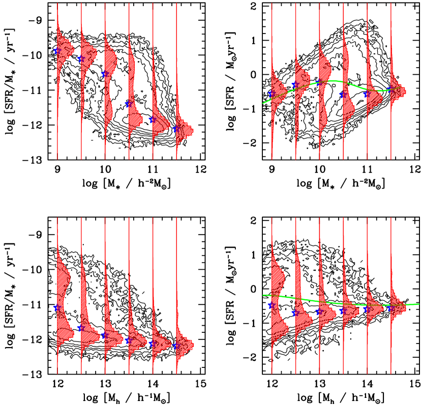
Figure 1.— The star formation rates (SFR; right-hand panels) and specific star formation rates (SSFR; left-hand panels) of central galaxies as function of their stellar mass $M_{*}$ (upper panels) and halo mass $M_{h}$ (lower panels). The contours in each panel show the number density distribution of the galaxies in logarithmic scale, with two neighboring levels differing by a factor two. The shaded vertical histograms in each panel are the SFR/SSFR distributions in logarithmic bins of stellar mass or halo mass with widths of $\pm 0.2\,$dex. The stars in each panel indicate the medians of these distributions, while the solid lines in the right-hand panels show our model prediction (see text).

In order to model the SFHs of central galaxies in dark matter halos of different masses, we need a reliable method to identify central galaxies, as well as accurate estimates of their SFRs, preferably across cosmic time. At low redshift, such information is available from galaxy group catalogs that can be used to represent dark matter halos. Here we make use of the SDSS group catalog constructed by Yang et al. (2007; hereafter Y07) using the adaptive halo-based group finder developed by Yang et al. (2005). The original catalog, based on SDSS Data Release 4 (DR4) is updated for DR7. The galaxies used for the group identifications are selected from the New York University Value-Added Galaxy catalog (NYU-VAGC; Blanton et al. 2005b), which is based on SDSS DR7 (Abazajian et al. 2009) but contains a number of improvements in data reduction. From the NYU-VAGC, we select all galaxies in the Main Galaxy Sample with an extinction-corrected apparent magnitude brighter than $r=17.72$, with redshifts in the range $0.01\leq z\leq 0.20$, and with a redshift completeness ${\cal C}_{z}>0.7$. The resulting galaxy catalog contains a total of $639,359$ galaxies, with a sky coverage of 7748 square degrees. A small fraction of galaxies have redshifts taken from the Korea Institute for Advanced Study (KIAS) Value-Added Galaxy Catalog (VAGC) (e.g. Choi et al. 2010). A total of $36,759$ galaxies, which do not have redshift measurements due to fiber collisions, are assigned the redshifts of their nearest neighbors. In the present paper, we use the group catalog ‘modelC’, which is constructed on the basis of all the galaxies (including those with assigned redshifts) and uses model magnitudes to estimate galaxy luminosities. In total our catalog contains $472,416$ groups, of which about $23,700$ have three member galaxies or more. Following Y07, we assign a halo mass to each group according to the ranking of its characteristic stellar mass, defined as the total stellar mass of all group members with $\>{}^{0.1}{\rm M}_{r}-5\log h\leq-19.5$, where $\>{}^{0.1}{\rm M}_{r}-5\log h$ is the absolute $r$-magnitude, K- and E-corrected to $z=0.1$, the typical redshift of galaxies in the SDSS redshift sample. The halo mass function adopted in the ranking is the model of Tinker et al. (2008), which assumes the WMAP7 cosmology and uses $\Delta=200$, with $\Delta$ the average mass density contrast within the halo (assumed to be spherically symmetric). Using the group catalogue, we divide galaxies into centrals and satellites; the most massive group member is identified as the central galaxy, while all other group members are assigned the status of satellite galaxy. As already mentioned above, in this paper we focus on the SFHs of central galaxies only.

The SFRs and the specific star formation rates, SSFRs (defined as the SFR divided by the stellar mass $M_{*}$), for individual galaxies adopted here are obtained from the data release of Brinchmann et al. (2004), who estimated the SFR and stellar mass for each galaxy by fitting the observed SDSS spectrum with a spectral synthesis model. About 94% of the galaxies used in our group identifications have estimated SFRs and SSFRs in the Brinchmann et al. data release (the vast majority of those lacking estimates are fiber collided galaxies with assigned redshifts).

Fig. 1 shows the SSFRs and SFRs of central galaxies versus stellar mass $M_{*}$ (upper panels) and halo mass $M_{h}$ (lower panels). In order to have a volume-limited sample of galaxies in stellar mass, we adopt, for given redshift $z$, the following stellar mass completeness limit,

$$\log[M_{*,{\rm lim}}/(\>h^{-2}{\rm M}_{\odot})]=$$

$${4.852+2.246\log D_{L}(z)+1.123\log(1+z)-1.186z\over 1-0.067z}\,$$

(see van den Bosch et al. 2008). In addition, we also apply the following halo mass completeness limit,

$$\log[M_{h,{\rm lim}}/(\>h^{-1}{\rm M}_{\odot})]=(z-0.085)/0.069+12\,$$ (2)

(see Yang et al. 2009b; hereafter Y09b). The contours shown in Fig. 1 are the number density distributions of central galaxies in ‘volume-limited’ samples complete in both stellar mass and halo mass according to $M_{*,{\rm lim}}$ and $M_{h,{\rm lim}}$ given above, i.e. for a given $z$ we only select systems with $M_{\ast}>M_{\ast,{\rm lim}}$ and $M_{h}>M_{h,{\rm lim}}$.

As is evident from the figure, the distributions in both SSFR and SFR are bimodal. For given $M_{\ast}$ or $M_{h}$, the central galaxies appear to be separated into two distinctive populations, one with high (S)SFRs (hereafter the “star forming” population) and the other with (S)SFRs that are more than 10 times smaller (hereafter the “quenched” population). To see this more clearly, we show in each panel, using the vertical shaded histograms, the distribution of galaxies within given logarithmic stellar mass (or halo mass) bins with widths of $\pm 0.2$dex. The star plotted on each of the histograms in each of the panels of Fig. 1 indicates the median value of the corresponding distribution.

Let us first focus on the SSFR - stellar mass relation shown in the upper left panel of Fig. 1. The SSFRs change significantly with stellar mass. Central galaxies with stellar masses $\gtrsim 10^{11}\>h^{-2}{\rm M}_{\odot}$ are predominantly quenched, while those with $M_{\ast}\lesssim 10^{9.5}\>h^{-2}{\rm M}_{\odot}$ are mostly star forming. Note, however, that if satellite galaxies were included, a significant fraction of the galaxies at the low mass-end would belong to the quenched population (e.g., van den Bosch et al. 2008; Peng et al. . 2012; Wetzel et al. 2012a,b). Galaxies with intermediate stellar masses show strong bi-modal distributions, with the quenched population becoming increasingly more important as the stellar mass increases. On average the SSFRs of central galaxies decrease with increasing stellar mass. Contrary to the SSFR, however, the total SFR distribution depicted in the upper right panel of Fig. 1 shows that the SFRs increase roughly linearly with stellar mass for the star-forming population, and with a somewhat slower rate for the quenched population.

Next, let us look at how SSFR and SFR depend on halo mass. As shown in the lower two panels of Fig. 1, galaxies in halos with masses $\gtrsim 10^{13.0}\>h^{-1}{\rm M}_{\odot}$ are dominated by the quenched population. However, this mode is much more ‘stretched’ in halo mass than in stellar mass. This is expected, because the stellar mass of central galaxies in massive halos increases only slowly with halo mass, $M_{\ast}\propto M_{h}^{0.22}$, as shown in Yang et al. (2008).

Finally, we emphasize once more that the above results are for central galaxies only. Had we included satellite galaxies, the quenched population would have been significantly more prevalent. In what follows these results will be used as local observational constraints to model the SFHs of central galaxies.

3. From conditional stellar mass function to star formation histories

In order to model the SFHs of central galaxies as function of halo mass, we first model how the stellar components in dark matter halos evolve with redshift. In this section, we first describe our model for the stellar mass-to-halo mass relation across cosmic time, based on the results published in Y12, followed by a description of how such a model can be extended to describe the SFHs of central galaxies as functions of halo mass.

3.1. The conditional stellar mass function of galaxies and its evolution

For a given dark matter halo, the total stellar mass it contains can be divided into three components: that in the central galaxy, that in the satellite galaxies, and that in the form of diffuse halo stars. In Y12 we have developed a self-consistent model for the conditional stellar mass function (CSMF), which describes the stellar mass distribution of galaxies in halos of a given mass, and its redshift evolution. This model properly takes into account that (i) subhalos are accreted at different times, and (ii) the properties of satellite galaxies may evolve after accretion. Since satellite galaxies were themselves centrals before accretion, the satellite population observed today serves as a “fossil record” for the formation and evolution of galaxies in dark matter halos over the entire cosmic history. Using the observed galaxy stellar mass functions out to $z\sim 4$, the conditional stellar mass function (hereafter CSMF) at $z\sim 0.1$, obtained from the SDSS galaxy group catalogue, and the two-point correlation function (2PCF) of galaxies at $z\sim 0.1$ as function of stellar mass, Y12 obtained the relationship between galaxy mass and halo mass over the entire cosmic history from $z\sim 4$ to $z=0.1$. This relation was then used to predict the assembly histories of different stellar mass components (centrals, satellites, and halo stars) as a function of halo mass. For completeness, we start with a brief description of the Y12 results that are relevant for the discussion that follows.

According to Y12, the CSMF of galaxies in halos of a given mass can be described by the functional form,

$$\Phi(M_{\ast}|M,z)=\Phi_{\rm c}(M_{\ast}|M,z)+\Phi_{\rm s}(m_{\ast}|M,z)\,,$$ (3)

where $\Phi_{\rm c}(M_{\ast}|M,z)$ and $\Phi_{\rm s}(m_{\ast}|M,z)$ are the contributions from the central and satellite galaxies, respectively. The CSMF of central galaxies is given by a lognormal distribution,

$$\Phi_{\rm c}(M_{\ast}|M,z)={1\over{\sqrt{2\pi}\sigma_{c}}}{\rm exp}\left[-{{(\log M_{\ast}/M_{\ast,c})^{2}}\over 2\sigma_{c}^{2}}\right]\,,$$ (4)

where $\log M_{\ast,c}$ is the expectation value of the (10-based) logarithm of the stellar mass of the central galaxy and $\sigma_{c}$ is the dispersion (see Y09b). For simplicity, $\sigma_{c}$ is assumed to be independent of halo mass, which has observational support (More et al. 2009). Following Y09b, the median stellar mass of the central galaxy is assumed to be a broken power-law,

$$M_{\ast,c}=M_{\ast,0}\frac{(M_{h}/M_{1})^{\alpha+\beta}}{(1+M_{h}/M_{1})^{\beta}}\,,$$ (5)

so that $M_{\ast,c}\propto M_{h}^{\alpha+\beta}$ ($M_{\ast,c}\propto M_{h}^{\alpha}$) for $M_{h}\ll M_{1}$ ($M_{h}\gg M_{1}$). This model contains four free parameters: an amplitude $M_{\ast,0}$, a characteristic halo mass, $M_{1}$, and two power indices , $\alpha$ and $\beta$. All four parameters may depend on redshift, as described below.

The CSMF for satellite galaxies can formally be written as,

$$\Phi_{\rm s}(m_{\ast}|M_{h},z)=\int\limits_{0}^{M_{h}}{\rm d}m_{a}\int\limits_{z}^{\infty}{{\rm d}z_{a}\over 1+z_{a}}\int\limits_{0}^{M_{h}}{\rm d}M_{a}\int\limits_{0}^{1}{\rm d}\eta~{}~{}~{}~{}~{}~{}~{}~{}~{}~{}$$

$$\Phi_{\rm e}(m_{\ast}|m_{a},z_{a},z)\,n_{\rm sub}(m_{a},z_{a}|M_{h},z)~{}~{}~{}~{}~{}~{}~{}~{}~{}~{}~{}~{}~{}~{}~{}$$

$$P(M_{a},z_{a}|M_{h},z)\,P(\eta)\,\Theta(p_{t}\,t_{\rm df}-\Delta t)\,,~{}~{}~{}~{}~{}~{}~{}~{}~{}~{}~{}~{}~{}$$ (6)

where $\Theta(x)$ is the Heaviside step function and $\Delta t$ is the time between redshifts $z_{a}$ and $z$. This model contains the following ingredients: (i) the accretion and mass distribution of subhalos, specified by $n_{\rm sub}(m_{a},z_{a}|M_{h},z)\,{\rm d}m_{a}\,{\rm d}\ln(1+z_{a})$ which is defined as the number of subhalos in a host halo of mass $M_{h}$ identified at redshift $z$ as a function of their accretion masses, $m_{a}$ and accretion redshifts, $z_{a}$ (Yang et al. 2011); (ii) the growth of the main branch of the host halo, specified by $P(M_{a},z_{a}|M_{h},z)$, which describes the probability that the main progenitor of a host halo of mass $M_{h}$ at redshift $z$ has a mass $M_{a}$ at $z_{a}$ (Zhao et al. 2009); (iii) the orbital distribution of accreted subhalos, specified by $P(\eta)$, where $\eta$ is the orbital circularity (Zenter et al. 2005); (iv) the disruption of subhalos during their evolution in the host, which is specified by the dynamical friction time $t_{\rm df}$ (Boylan-Kolchin et al. 2008); (v) the relative disruption rate of satellite galaxies with respect to subhalos, which is characterized by a free parameter $p_{t}$: $p_{t}=\infty$ corresponds to no tidal stripping/disruption of satellite galaxies, while $p_{t}=0$ corresponds to instantaneous disruption of all satellites, and finally (vi) the evolution of a satellite from its time of accretion until the time corresponding to redshift $z$, specified by $\Phi_{\rm e}(m_{\ast}|m_{a},z_{a},z)$, the probability for a subhalo of mass $m_{a}$ and accretion redshift $z_{a}$ to host a satellite galaxy of stellar mass $m_{\ast}$ at redshift $z$. In Y12 it is assumed that

$$\Phi_{\rm e}(m_{\ast}^{\prime}|m_{a},z_{a},z)={1\over{\sqrt{2\pi}\sigma_{c}^{\prime}}}{\rm exp}\left[-{{(\log m_{\ast}^{\prime}/{\overline{m}}_{\ast}^{\prime})^{2}}\over 2\sigma_{c}^{\prime 2}}\right]\,.$$ (7)

The dispersion, $\sigma_{c}^{\prime}$, is assumed to be the same as $\sigma_{c}$, while the median is written as

$${\overline{m}}_{\ast}^{\prime}=(1-c)m_{\ast,a}+cm_{\ast,z}\,,$$ (8)

where $m_{\ast,a}$ is the stellar mass of the satellite at the accretion time $z_{a}$, $m_{\ast,z}$ is the stellar mass of the central galaxy of a halo of mass $m_{a}$ at time $z$, and $c$ is a free parameter. Thus, if $c=0$ then ${\overline{m}}_{\ast}^{\prime}=m_{\ast,a}$ so that the stellar mass of a satellite is equal to its original mass at accretion. Physically this corresponds to a picture in which a satellite galaxy is instantaneously quenched upon accretion. On the other hand, if $c=1$ then ${\overline{m}}_{\ast}^{\prime}=m_{\ast,z}$ so that the stellar mass of a satellite is the same as that of a central galaxy in a halo of mass $m_{a}$ at redshift $z$. This corresponds to the assumption made in SHAM; in other words, by setting $c=1$ we are effectively mimicking SHAM. Note that for $c=0$ we have that $\Phi_{\rm e}(m_{\ast}^{\prime}|m_{a},z_{a},z)$ has the same form as the CSMF of central galaxies at the accretion redshift $z_{a}$.

At any particular redshift, the above model of the CSMF is fully described by the following seven free parameters: $M_{\ast,0}$, $M_{1}$, $\alpha$, $\beta$, $\sigma_{c}$, $p_{t}$ and $c$. In order to describe the evolution of the galaxy distribution over cosmic time, Y12 assumed the following redshift dependence for the model parameters:

$$\log[M_{\ast,0}(z)] = \log(M_{\ast,0})+{\gamma_{1}z}$$

$$\log[M_{1}(z)] = \log(M_{1})+{\gamma_{2}z}$$

$$\alpha(z) = \alpha+{\gamma_{3}z}$$

$$\log[\beta(z)] = {\rm min}[\log(\beta)+{\gamma_{4}z}+{\gamma_{5}z^{2}},2]$$ (9)

$$\sigma_{c}(z) = {\rm max}[0.173,0.2z]$$

$$p_{t}(z) = p_{t}$$

$$c(z) = c\,.$$

The model is thus specified by a total of 11 free parameters, four that describe the CSMF at $z=0$, five that describe their evolution with redshift, and two ($c$ and $p_{t}$) that describe the evolution of satellite galaxies.

Once the free parameters are given, the formalism described above allows one to predict the stellar mass functions as well as correlation functions of galaxies. Thus, one can use observational data on the stellar mass functions (SMFs) and 2-point correlation functions (2PCFs) to constrain the model parameters. Y12 used a Markov Chain Monte Carlo (hereafter MCMC) method to explore the likelihood function in the 11-dimensional parameter space, adopting the WMAP7 cosmology. In particular, two types of analysis were carried out for comparison. The first uses the SMFs at different redshifts together with the 2PCFs of galaxies at low-$z$ as constraints; the second uses the SMFs at different redshifts together with the CSMFs at low $z$. Since both analyses gave very similar results, in this paper we only use the results based on the latter analysis. Furthermore, Y12 used two sets of high redshift stellar mass functions, one obtained by Perez-Gonzalez et al. (2008; referred to as SMF1), and the other obtained by Drory et al. (2005; referred to as SMF2). Since these two data sets reveal quite large discrepancies with respect to each other and dominate over all the uncertainties in our model ingredients, we will present results separately for both of them.

3.2. The growth of stellar components in dark matter halos

Once the redshift-dependent CSMFs are obtained, one can predict the growth of the stellar masses of both central and satellite galaxies along the main branch of their dark matter halos. The median stellar mass at redshift $z$ of a central galaxy that at redshift $z_{0}\leq z$ is located in a host halo of mass $M_{0}$ can be written as

$$M_{\ast,c}(z|M_{0},z_{0})=M_{\ast,c}(M_{a},z)\,.$$ (10)

Here, as before, $M_{a}$ is the median mass at redshift $z\geq z_{0}$ of the main progenitor of a host halo of mass $M_{0}$ at redshift $z_{0}$. The median total stellar mass of the surviving satellite galaxies in the main branch can be obtained by integrating the CSMF of satellite galaxies:

$$m_{\ast,s}(z|M_{0},z_{0})=\int{\rm d}\log m_{\ast}\,m_{\ast}\,\Phi_{\rm s}(m_{\ast}|M_{a},z)\,.$$ (11)

Thus, once the assembly history of a dark matter halo is known, it is straightforward to use the CSMF to obtain the corresponding assembly histories of the stellar components. In addition, one can also estimate the total mass of all satellite galaxies that have been accreted into the main branch, which includes stellar mass in both the currently surviving satellites and those that have been cannibalized by the central galaxy or disrupted by the tidal field. This is given by

$$m_{\ast,{\rm acc}}(z|M_{0},z_{0})=\int_{z_{0}}^{z}{{\rm d}z_{a}\over(1+z_{a})}\int{\rm d}\log m_{\ast}\,m_{\ast}~{}~{}~{}~{}~{}~{}~{}~{}~{}~{}$$ (12)

$$\Phi_{\rm e}(m_{\ast}|m_{a},z_{a},z)\,n_{\rm sub}(m_{a},z_{a}|M_{0},z_{0})\,.~{}~{}~{}~{}~{}~{}~{}~{}~{}~{}~{}~{}~{}~{}$$

Note that $\Phi_{\rm e}$ accounts for evolution in the stellar masses of satellite galaxies after accretion due to star formation, stellar mass stripping and mass loss due to stellar evolution.

The difference between $m_{\ast,{\rm acc}}$ and $m_{\ast,s}$ gives the total mass of (destroyed) satellites that are either cannibalized by the central or disrupted by the tidal field. As shown in Y12, the mass in this stellar component in a massive cluster can be much larger than that of the central galaxy. Hence, a significant fraction of the total stellar mass from the disrupted satellite galaxies cannot be associated with the central galaxy, but instead has to be in the form of diffuse halo stars. Unfortunately, what fraction of stars in a halo is associated with such a diffuse halo component (also called ‘intra-cluster light’ in the case of clusters) is still poorly constrained observationally (e.g. Gonzalez et al. 2005 Seigar et al. 2007), so that it remains unclear what fraction of the ‘destroyed’ satellite is cannibalized by the central vs. added to the stellar halo (e.g. Purcell et al. 2007; Kang & van den Bosch 2008; Yang et al. 2009a). Two extreme assumptions can be made for the contribution of the destroyed satellites to the growth of the central: (i) minimum (zero) contribution; and (ii) maximum contribution, where the contributed mass is equal to either the mass growth of the central or the total mass of destroyed satellites, whichever is smaller, in a given time interval.

In general, the growth (evolution) of the central galaxies consists of the following three contributions: (i) its in situ star formation; (ii) the accretion of stars from satellite galaxies; and (iii) its passive evolution (mass loss). The model described above for the stellar mass assembly histories of central galaxies and the possible contribution from accreted satellites can therefore be used to infer the SFH of central galaxies:

$$SFR(z) = \frac{{\rm d}M_{\ast,c}(z)}{{\rm d}t}-f_{\rm acc}\left\{\frac{{\rm d}[m_{\ast,{\rm acc}}(z)-m_{\ast,s}(z)]}{{\rm d}t}\right\}$$ (13)

$$+ \frac{{\rm d}M_{\ast,{\rm loss}}(z)}{{\rm d}t}\,,$$

where

$$\frac{{\rm d}M_{\ast,{\rm loss}}(z)}{{\rm d}t}=\int^{t(z)}_{0}\frac{{\rm d}M_{\ast,c}(z)}{{\rm d}t_{1}}\,\frac{{\rm d}f_{\rm passive}(t(z)-t_{1})}{{\rm d}t}{\rm d}t_{1}\,,$$ (14)

is the stellar mass loss due to the passive evolution of stars. Corresponding to the two extreme cases for the contribution of the destroyed satellites are two extreme estimates for the SFH: (i) maximum star formation (hereafter ‘MAX’), in which the stellar mass growth of central galaxies is entirely due to in situ star formation, i.e. $f_{\rm acc}=0$; (ii) minimum star formation (hereafter ‘MIN’), in which the contribution from accreted satellites is maximized ($f_{\rm acc}=1$) or $SFR(z)=0$ if $f_{\rm acc}=1$ leads to $SFR(z)<0$.

The stellar mass loss due to passive evolution is accounted for via the function $f_{\rm passive}(t)$, which describes the mass fraction of stars that at time $t$ after their formation is still in the form of stars. We obtain $f_{\rm passive}(t)$ from the stellar population model of Bruzual & Charlot (2003), kindly provided by Stephane Charlot (private communication). Throughout this paper we adopt the results for the Kroupa (2001) IMF, which asymptotes to $f_{\rm passive}\sim 0.57$ at late stages of evolution. For Chabrier (2003) and Salpeter (1955) IMFs, these asymptotical values are $\sim 0.54$ and $\sim 0.70$, respectively. We have tested that changing the IMF from Kroupa to Chabrier or Salpeter results in changes in the SFRs of $\lesssim 0.1\,{\rm dex}$, much smaller than the uncertainties from other sources, e.g., the use of SMF1 or SMF2.

4. The Star Formation Histories of Central Galaxies

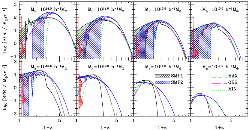
Figure 2.— The star formation rates (SFRs) of central galaxies as a function of redshift in halos of different present-day masses, as indicated in each panel. Black and blue shaded regions reflect the model predictions obtained using SMF1 and SMF2, respectively. For each of these two cases, the shaded areas mark the SFRs between the MIN and MAX assumptions (see text for details), which become more and more similar at higher redshift and for lower mass halos. In the panels for halos with $M_{h}\geq 10^{12}\>h^{-1}{\rm M}_{\odot}$, local observational constraints from SDSS are shown as the vertical shaded histograms (distributions) and stars (median). The dotted, dashed, and long-dashed lines are the MIN, MAX and OBS fits to the SFHs discussed in the text.

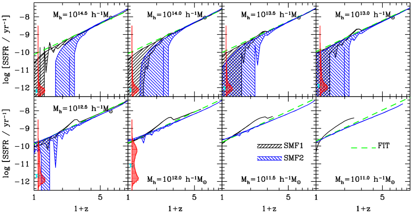
Figure 3.— Same as Fig, 2, except that here we show the specific star formation rates (SSFRs) of central galaxies as function of redshift. The dashed line is the model fit of Eq. (4.1), which accurately describes the SSFRs of central galaxies prior to their quenching (see text for detailed discussion).

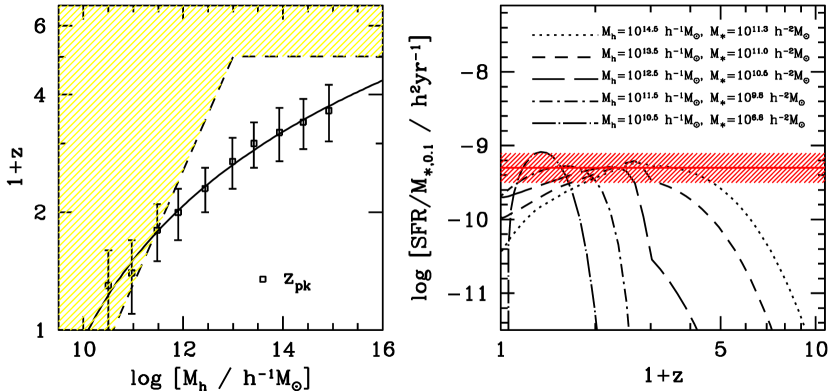
Figure 4.— Left-hand panel: the peak redshift of the SFR as a function of present-day host halo mass. Data points with error bars are the rough estimations of the peak redshifts from the SFHs shown in Fig. 2, with the errorbars reflecting the redshift interval over which the SFR is within 10% of its peak value. The solid line is a fit to the data points (Eq. [16]). As an illustration, we also show using the shaded region where our SFH results are obtained from extrapolations. Right-hand panel: the star formation histories of central galaxies, normalized by the stellar masses of the central galaxies at redshift $z=0.1$. Over about 4 orders of magnitude in halo mass and stellar mass, these normalized SFHs peak at $10^{-9.3}h^{2}{\rm yr}^{-1}$ (within $\sim 0.2\,$dex), as indicated by the horizontal band.

Applying the model outlined in Section 3.2 from high to low redshifts, we obtain the SFHs of central galaxies in halos of different masses. Figs. 2 and  3 show the median SFRs and SSFRs as a function of redshift for the centrals in halos of different final masses, as indicated in each panel. In each panel, the black and blue lines correspond to the results obtained using SMF1 and SMF2, respectively. For each set of observational data (SMF1 or SMF2), predictions based on both the MIN and MAX assumptions are shown, connected by the corresponding shaded areas. As described in Section 3.2, MIN and MAX correspond to the maximum and minimum (zero) contribution of satellites to the mass growth of central galaxies, respectively, so that they represent the lower and upper limits on the SFRs of central galaxies. As one can see, at $z>2$, these upper and lower limits are always very similar for halos of all masses. This indicates that the growth of stellar mass at these high redshifts is completely dominated by in situ star formation (see Y12). At lower redshift, the MIN and MAX assumptions results in fairly different SFRs, especially for halos with $M_{h}\gtrsim 10^{12}\>h^{-1}{\rm M}_{\odot}$. In these halos, mass growth due to the accretion of satellite galaxies could be responsible for a significant fraction of the final stellar mass of centrals. In the absence of accurate estimates for the mass components in halo stars, it will be difficult to discriminate between these MIN and MAX models, and therefore to tighten the constraints.

However, as shown in Section 2, the (S)SFRs of low-$z$ central galaxies can be estimated for halos of different masses directly from observational data. This provides a direct constraint on the SFH at $z\sim 0$. In Figs. 2 and  3 the vertical shaded histograms show the local observational constraints for halos with masses $\gtrsim 10^{12}\>h^{-1}{\rm M}_{\odot}$. Results for halos with lower masses are not available from the group catalog (see Y07). In general, the median (S)SFRs obtained directly from the SDSS group catalog (indicated by crosses) nicely falls within the shaded area, between the upper and lower limits corresponding to the MIN and MAX assumptions, indicating that the SFRs obtained from our model are consistent with the results obtained directly from the SDSS groups. However, there are two exceptions: our model under-predicts the median (S)SFR of centrals in massive halos with $M_{h}\gtrsim 10^{14.0}\>h^{-1}{\rm M}_{\odot}$ in the case of SMF2, and over-predicts the median (S)SFRs of central galaxies in halos with $M_{h}=10^{12}\>h^{-1}{\rm M}_{\odot}$. In the case of SMF2, the model prediction of the (S)SFR for central galaxies in massive halos with $M_{h}\gtrsim 10^{14.0}\>h^{-1}{\rm M}_{\odot}$ is well below the median (S)SFRs obtained from the group catalog. This happens because the use of SMF2 slightly over-predicts the number density of very massive galaxies at redshift $z\sim 1$ in comparison to that obtained directly from the SDSS data.

For halos with $M_{h}\sim 10^{12}\>h^{-1}{\rm M}_{\odot}$ the models based on both SMF1 and SMF2 predict a median SSFR at $z=0.1$ of $\sim 10^{-10}{\rm yr}^{-1}$. In contrast, the SSFRs obtained directly from the SDSS data reveals two distinctive populations: a star-forming population, whose SSFRs peak at $\sim 10^{-10.2}\,{\rm yr}^{-1}$ and a quenched population with $\langle{\rm SSFR}\rangle\sim 10^{-11.8}\,{\rm yr}^{-1}$. Thus, it appears that our model fails to account for the quenched population. We suspect that this is caused by two effects. First, due to contamination in the group finder, some of the red centrals in the group catalog are actually satellite galaxies. However, as shown in Y07, this contamination fraction is about $\lesssim 10\%$, which is not sufficient to explain the relatively large fraction of quenched centrals in groups with $M_{h}\sim 10^{12}\>h^{-1}{\rm M}_{\odot}$. Second, some of the quenched centrals may be a population of galaxies that is located in the outskirts of a more massive halos which it traversed in the past. Star formation in such galaxies is likely to have experienced the same quenching as satellites during their journeys through the massive halos (Wetzel et al. 2013). Numerical simulations suggest that such a population is expected, as some of the low-mass halos located near massive ones have indeed passed through massive halos at least once in the past (e.g. Lin et al. 2003; Gill, Knebe & Gibson 2005; Wang et al. 2009a; Ludlow et al. 2009). Observationally, Wang et al. (2009b) found that many of the red dwarf galaxies not contained within the virial radii of massive halos are located within three virial radii from nearby massive halos, consistent with the idea that they were quenched when they passed through their massive neighbor (see also Geha et al. 2012). If such a population also exist for galaxies with stellar masses $\sim 10^{10}\>h^{-2}{\rm M}_{\odot}$, it might be possible to explain the quenched population of centrals in galaxy groups with masses $\sim 10^{12}\>h^{-1}{\rm M}_{\odot}$. Such a population is missed in our model, where all halos that have once been accreted into a host halo are considered as subhalos hosting satellite galaxies. Clearly, detailed analysis is needed in order to quantify the contribution of this kind of “passing-through” galaxies to the quenched population (see e.g., Wetzel et al. 2013).

4.1. Analytical Model

Let us now move on to a quantification of the predicted SFHs. We first focus on the SSFRs of central galaxies. As one can see from Fig. 3, at high $z$ the SSFRs roughly reveal a power law dependence on redshift. The results obtained from SMF1 and SMF2 are remarkably similar, and are well described by

$$\log({\rm SSFR}/{\rm yr}^{-1}) = 2.5\log(1+z)$$

$$- 0.12\log(M_{h}/\>h^{-1}{\rm M}_{\odot})-12.0\,,~{}~{}~{}~{}~{}$$

which is indicated as the dashed line in each of the panels in the figure. In small halos with $M_{h}\lesssim 10^{12.0}\>h^{-1}{\rm M}_{\odot}$, Eq. (4.1) holds for the entire SFH. In halos with $M_{h}\gtrsim 10^{12.5}\>h^{-1}{\rm M}_{\odot}$, however, Eq (4.1) holds only for $z>z_{\rm pk}$, where $z_{\rm pk}$ is defined as the redshift at which the SFR peaks (see below). Eq. (4.1) indicates that the SSFR of central galaxies depends only weakly on galaxy mass. For example, central galaxies in halos with $M_{h}=10^{11}$ and $10^{12}\>h^{-1}{\rm M}_{\odot}$ have similar SSFRs, even though their stellar masses differ by more than an order of magnitude (cf. Fig. 13 in Y12). The dependence of SSFR on redshift is much stronger, increasing by a factor of about 6 from $z=1$ to $z=3$. Interestingly, this scaling of the SSFR with halo mass and redshift is almost identical to that of the specific mass accretion rate of dark matter halos, which scales as $\dot{M}_{h}/M_{h}\propto M_{h}^{0.15}\,(1+z)^{2.25}$ (Dekel et al. 2009; see also McBride et al. 2009; Fakhouri et al. 2010 for similar results obtained from N-body simulations). This suggests that the SFR of star-forming (i.e., non-quenched) central galaxies is regulated by the rate at which their host halos accrete mass, in excellent agreement with a number of recent studies (e.g., Dutton, van den Bosch & Dekel 2010; Bouché et al. 2010; Davé, Finlator & Oppenheimer 2012).

The SFRs in Fig. 2 show that $z_{\rm pk}$ increases with increasing stellar mass (or halo mass), indicating that more massive centrals are quenched earlier (a manifestation of what is often called ‘downsizing’). We have estimated $z_{\rm pk}$ as a function of halo mass, $M_{h}$, using the SFHs obtained from both SMF1 and SMF2. The open squares in the left-hand panel of Fig. 4 show the average between SMF1 and SMF2, while the errorbars are obtained from the points where the SFH is about 10% of the peak value. Using the following functional form to fit the data,

$$z_{\rm pk}=\max[a(\log M_{h}-b),0]\,,$$ (16)

we obtain $a=0.568$ and $b=10.10$. This fitting function is shown in the left-hand panel of Fig. 4 as the solid line.

In addition to $z_{\rm pk}$ increasing with halo mass, the actual SFR at the peak redshift also increases with halo mass. As is evident from Fig. 2, this halo mass dependence becomes weaker in more massive halos. This kind of halo mass dependence is also seen for the luminosities and stellar masses of central galaxies at low redshift (see, e.g., Y09b). Interestingly, if we normalize the SFRs of the central galaxies by their stellar masses at $z=0.1$, the peak amplitude becomes virtually independent of halo mass and stellar mass! This is demonstrated in the right-hand panel of Fig. 4, which plots $\log[SFR/M_{{\ast},0.1}]$ as function of redshift for five different values of the present-day halo mass, as indicated. The peak amplitude is about $\log[{\rm SFR}/M_{{\ast},0.1}\times h^{-2}{\rm yr}]=-9.3$, which is indicated by the horizontal line. The hatched, horizontal band covers $\pm 0.2$ dex around this line and roughly represents the uncertainty in the estimate of the SFR and stellar mass. Thus, central galaxies with stellar mass $M_{\ast,0.1}$ at $z=0.1$, have a maximum SFR

$${{\rm SFR}_{\rm pk}\over[{\rm M}_{\odot}\,{\rm yr}^{-1}]}={M_{\ast,0.1}\over 10^{9.3}\>h^{-2}{\rm M}_{\odot}}\,$$ (17)

at redshift $z_{\rm pk}$ given by Eq. (16). These equations hold for central galaxies covering over 4 orders of magnitude in both halo mass and stellar mass. Note that our modeling here is based mainly on results obtained from SMF1. The results obtained from SMF2 are qualitatively similar, and shown in the Appendix for comparison.

Motivated by the general appearance of the SFHs, we use the following functional form to model the SFHs of central galaxies as function of halo mass and redshift:

$${\rm SFR}(M_{h},z)={\rm SFR}_{\rm pk}\times\exp\left\{-{\log^{2}[(1+z)/(1+z_{\rm pk})]\over 2\sigma^{2}(z_{\rm pk})}\right\}\,,$$ (18)

where $\sigma(z_{\rm pk})$ describes the decay of the SFR with respect to the peak. By trial-and-error, we find that a simple power-law scaling with $(1+z_{\rm pk})$ can adequately describe the SFHs. For $z\geq z_{\rm pk}$ we obtain

$$\sigma(z_{\rm pk})=0.0576(1+z_{\rm pk})^{0.707}\,,$$ (19)

where the parameters are obtained using least squares fitting to the SFHs at high redshifts. The differences between the SMF1 and SMF2 model predictions are used as weights in the fitting. For $z<z_{\rm pk}$ we obtain different power-law scalings:

$$\sigma(z_{\rm pk})=\left\{\begin{array}[]{ll}0.0762(1+z_{\rm pk})^{0.523}{}{}{}&\mbox{(OBS)}\\ 0.0706(1+z_{\rm pk})^{0.940}{}{}{}&\mbox{(MAX)}\\ 0.317(1+z_{\rm pk})^{-2.10}{}{}{}&\mbox{(MIN)}\end{array}\right.\,.$$ (23)

Here the case marked ‘OBS’ assumes that the SFHs at low-$z$ are constrained by the SFR measurements from the SDSS groups using least squares fitting to the median SFRs of central galaxies as a function of stellar mass (asterisks in upper right-hand panel of Fig. 1). The case marked ‘MAX’ assumes that all stars in central galaxies are formed in situ, in which case the stellar mass of central galaxies as function of redshift, $z_{0}$, follows from integrating the SFH and taking into account the effect due to passive evolution,

$$M_{\ast}(z_{0})=\int_{0}^{t_{z_{0}}}{\rm SFR}_{\rm MAX}(t)\,f_{\rm passive}(t_{z_{0}}-t)~{}{\rm d}t\,.$$ (24)

Here $t_{z_{0}}$ is the age of the universe at redshift $z_{0}$ and $1-f_{\rm passive}(\Delta t)$ is the mass fraction of stars formed that a time $\Delta t$ later has been returned to the IGM due to stellar (passive) evolution. By definition, $M_{\ast}(z_{0}=0.1)=M_{\ast,0.1}$, which is used to obtain the two parameters in Eq.(23) for the ‘MAX’ case. For the ‘MIN’ case, the two parameters in Eq. (23) are obtained from the corresponding low-redshift SFHs given by SMF1.

The resulting SFH model predictions are plotted as the long-dashed (OBS), dashed (MAX) and dotted lines (MIN) in Fig. 2. Thus, Eq. (18) describes the median SFH for central galaxies with a given stellar mass at redshift $z=0.1$. For halos of a given mass $M_{h}$, one can first obtain the corresponding $M_{\ast,0.1}$ using Eqs. (5) and (3.1), and then obtain the SFH from Eq. (18). The uncertainties in the SFH model may be gauged from the differences between the model predictions for SMF1 and SMF2, and between the results for the two extreme assumptions, MIN and MAX (see Fig. 2). As pointed out in Y12, at the present the uncertainties in the CSMF modeling are dominated by systematic errors between SMF1 and SMF2 (see Fig. 14 in Y12), rather than by the statistical errors in the data. Note that our model is obtained from observational measurements of stellar mass functions that are limited in both redshift ($z\lesssim 4$ for SMF1 and $z\lesssim 5$ for SMF2) and stellar mass (see Fig.3 in Y12). Results beyond these redshift and/or stellar mass ranges are in general obtained by extrapolation, and therefore less reliable. As an illustration, we show, in the left panel of Fig. 4 using the shaded region, where our SFH results are obtained from extrapolations.

Finally, we emphasize that our model for the SFHs is based on the assembly histories of central galaxies in halos of a given final mass, and it is expected to work well only for centrals with mass assembly histories close to the median. Deviations from the median are expected to result in deviations of the inferred SFHs from the model prediction and may in fact be the main source of the scatter seen in Fig. 1. In a forthcoming paper, we will come back to the modeling of this scatter together with the SFHs of satellite galaxies.

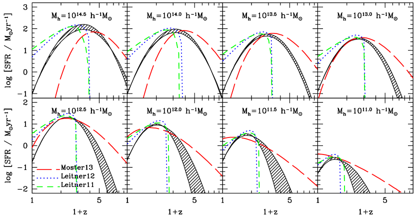
Figure 5.— The SFHs of central galaxies, similar to Fig. 2 but here our model predictions are compared with the results obtained in a few recent papers. The lower and upper boundaries of the shade areas are our OBS model predictions of the SFHs for central galaxies based on SMF1 with the SFR described by Eq. (18), and SMF2 with the SFR described by Eq. (A3), respectively. The dashed, dotted and long dashed lines in each panel are model predictions based on Leitner & Kravtsov (2011), Leitner (2012) and Moster et al. (2013), respectively. See text for a detailed discussion.

4.2. How to Use the Model

As a summary, the following is a brief description of the procedure for obtaining the median SFH for a central galaxy in a halo of a given mass:

1. Start from a halo with mass $M_{h}$ at low redshift (e.g. $z\sim 0.1$). Use Eqs. (17) and (40) in Yang et al. (2012), which are the relations adopted in this paper, or use Eq.  (20) of Yang et al. (2009), which was obtained directly from the SDSS group catalog, or use any other stellar mass - halo mass relation for central galaxies, to obtain the stellar mass, $M_{\ast,0.1}$, of the central galaxy at $z\simeq 0.1$;

2. Use Eq. (16) to obtain the redshift, $z_{\rm pk}$, at which the SFR peaks;

3. Use Eq. (17) to get the peak value of the SFR, ${\rm SFR}_{\rm pk}$;

4. Finally, the median SFH of the central galaxy is described by Eq. (18) with $\sigma(z_{\rm pk})$ given by Eqs. (19) and (23) for the case labelled ‘OBS’.

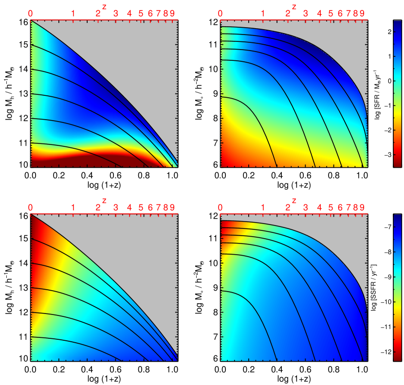
Figure 6.— Maps of our model predictions for the star formation rates (SFR; upper panels) and specific star formation rates (SSFR; lower panels) of central galaxies as functions of halo mass (left-hand panels) or stellar mass (right-hand panels) and redshift. The vertical bars on the right-hand side indicate the corresponding color-coding, where the SFR and SSFR are expressed in units of ${\rm M}_{\odot}{\rm yr}^{-1}$ and ${\rm yr}^{-1}$, respectively. The solid curves in each of the panels show the median growth of halo mass (left-hand panels) and stellar mass (right-hand panels) along the main branch of halos with different present-day masses.

4.3. Comparison with some recent results

As pointed out in the introduction, there are a number of recent studies that, similar to this paper, modelled the SFHs of galaxies as function of halo mass. All these studies make use of SHAM (or a modified version thereof), together with halo merger trees generated from N-body simulations, to make predictions for the mass growth and SFH of galaxies (e.g., Moster et al. 2013; Behroozi et al. 2012, 2013; Wang et al. 2012). In all these analyses, assumptions have to be made regarding the evolution of satellite galaxies, in particular regarding the contribution of satellite accretion to the mass assembly of central galaxies. Although the results from all these analyses are qualitatively similar to each other and to our results, there are substantial, quantitative differences. In this subsection, we make a quantitative comparison between our results and those obtained by Moster et al. (2013).

Fig. 5 shows our model predictions of the SFHs for central galaxies. The lower and upper boundaries of the shaded areas are our model predictions based on SMF1 (the same as the long dashed lines in Fig. 2) and SMF2 (the same as the long dashed lines in Fig. 15), respectively. The long-dashed line shown in each panel is the result obtained with the fitting formula provided by Moster et al. (2013). The Moster et al. results are obtained by assuming a WMAP7 cosmology and a Chabrier (2003) IMF; these are sufficiently similar to the cosmology and IMF adopted here, that a direct comparison is justified. Within the uncertainty ($\sim 0.2\,{\rm dex}$ in the SFH), the peaks in the SFHs of Moster et al. (2013) are roughly consistent with our model predictions. However, at high-$z$ their SFHs are higher than ours while at low-$z$ and for massive halos, the Moster et al. SFHs are lower than our model predictions. These differences, especially those at low-$z$, most likely comes from the different treatment of satellite galaxies. Moster et al. (2013) assume that 20% of the stellar mass of accreted satellite galaxies ‘escapes’ from the central galaxy, ending up as diffuse halo stars. If we add such a prescription to our model, we predict a low-$z$ behavior that is very similar to that of Moster et al., although we find that a ‘satellite disruption fraction’ of $\sim 45$%, rather than $20$%, yields results that are in better agreement with observational constraints on the SFHs.

It is also interesting to compare our results to those of Leitner & Kravtsov (2011) and Leitner (2012), who modeled the stellar mass growth in star-forming galaxies using the observed SFR-stellar mass relations at different redshifts. The short-dashed and dotted lines in Fig. 5 show the model predictions of Leitner & Kravtsov (2011) and Leitner (2012), respectively. Although their models predict SFH peaks that are very similar to our model predictions, their models predict SFRs at low (high) redshifts that are significantly higher (lower). The difference at low-$z$ is expected, because their models only describe star-forming galaxies, while our models are for the general population. At high-$z$, the results of Leitner & Kravtsov (2011) and Leitner (2012) are not obtained directly from observational data but rather from extrapolations of the low-$z$ data to higher redshifts. We therefore suspect that the difference between their results and ours reflects an amplification of the uncertainties in their SFR-stellar mass relations at lower $z$.

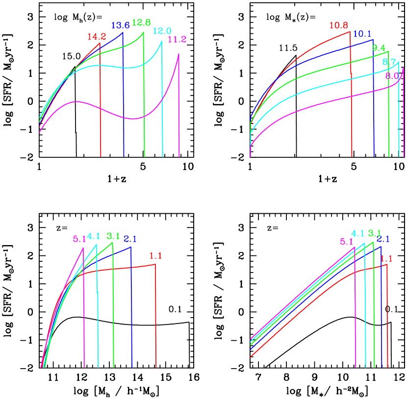
Figure 7.— Model predictions for the star formation rates of central galaxies. The upper panels show the SFRs of central galaxies as function of redshift for different halo masses (upper left-hand panel) and different stellar masses (upper right-hand panel), as labelled. The lower panels show the SFRs of central galaxies as functions of halo mass (left-hand panel) and stellar mass (right-hand panel) at different redshifts, as labelled. All these curves are either vertical or horizontal cuts through the SFR maps shown in the upper panels of Fig. 6. In each of the four panels, the vertical cut-offs in the curves correspond to median main branch mass of a halo with present day mass $M_{h}=10^{16}\>h^{-1}{\rm M}_{\odot}$.

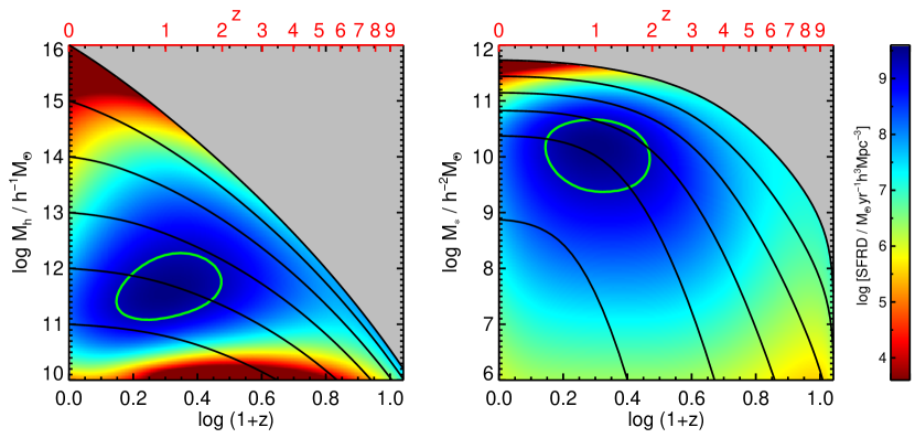
Figure 8.— Maps of our model predictions for the star formation rate density (SFRD) of central galaxies. The color coding used is indicated in the vertical bar on the right-hand site. These SFRDs are normalized to be the mass density of stars formed per unit $\log M_{h}$ per unit $\log(1+z)$ (left-hand panel) or per unit $\log M_{\ast}$ per unit $\log(1+z)$ (right-hand panel), and are expressed in units of ${\rm M}_{\odot}{\rm yr}^{-1}[\>h^{-1}{\rm Mpc}]^{-3}$. The contours in the two panels enclose a region that contributes 50% of the total stars formed in the universe. As in Fig. 6, the solid curves show the median growth of halo mass (left-hand panel) and stellar mass (right-hand panel) along the main branch of halos with different present-day masses.

5. Model predictions

In this section we use our model for the SFHs of central galaxies as function of halo mass to make a number of predictions that provide valuable insight into how star formation proceeds in the Universe. Note that throughout this section, unless specified otherwise, our model predictions are made from observational constrained SFHs obtained from SMF1 (as SMF1 shows better agreement with the SFR measurements at $z=0.1$ than SMF2).

5.1. The star formation rate as a function of halo mass and redshift

Let us first look at the SFR maps in the $M_{h}$ - $z$ and $M_{\ast}$ - $z$ spaces, shown in the upper row of panels of Fig. 6. For reference, the solid lines show the growth of the host halo mass (left-hand panel) and the growth of stellar mass of the central galaxies (right-hand panel). These relations are obtained from the halo mass accretion model of Zhao et al. (2009) and from the median stellar mass - halo mass relation for central galaxies obtained by Y12 (Eq. [10]), respectively. Results are only shown for systems that have $M_{h}\leq 10^{16}\>h^{-1}{\rm M}_{\odot}$, since more massive halos are extremely rare. As one can see, the SFRs peak in massive galaxies with $M_{\ast}\sim 10^{11.0}\>h^{-2}{\rm M}_{\odot}$ in halos with $M_{h}\sim 10^{13.5}\>h^{-1}{\rm M}_{\odot}$ at redshift $z\sim 2.5$, and the peak star formation rate is about $100{\rm M}_{\odot}\,{\rm yr}^{-1}$. At low redshift ($z\lesssim 0.5$), SFRs are highest in galaxies with $M_{\ast}\sim 10^{10.0}\>h^{-2}{\rm M}_{\odot}$ in halos with $M_{h}\sim 10^{12}\>h^{-1}{\rm M}_{\odot}$. Also there is a lower halo mass limit at $\lesssim 10^{10.5}\>h^{-1}{\rm M}_{\odot}$, below which the star formation is low over the entire redshift range. Note that these results are in good qualitative agreement with the results of Behroozi et al. (2012).

In addition to the SFR, in the lower panels of Fig. 6 we show the corresponding SSFR maps. In general the SSFR maps show a smooth gradient in redshift, being higher at higher redshift. At high $z$, the SSFR depends only weakly on halo mass and galaxy mass. Only after the peak redshift of the SFR (see Eq. [16]), does the SSFR decrease more rapidly in more massive galaxies hosted by more massive halos.

To better illustrate the behavior of the SFRs, it is useful to show some horizontal and vertical cuts of the SFR maps. The upper panels of Fig. 7 show the SFR as a function of redshift for central galaxies in different mass halos (upper-left panel) and for central galaxies of different stellar masses (upper-right panel). In the lower panels, we plot the SFR as a function of halo mass (lower-left panel) and stellar mass (lower-right panel) at different redshifts, as indicated. The sharp cut-offs in each panel correspond to the median main branch mass of a massive halo with $M_{h}=10^{16}\>h^{-1}{\rm M}_{\odot}$ at $z=0$, beyond which the abundance of systems is negligibly small.

A number of interesting characteristics are evident from these plots. First, for central galaxies in massive halos with $M_{h}\gtrsim 10^{12}\>h^{-1}{\rm M}_{\odot}$, the SFR increases monotonically with redshift (see the upper-left panel of Fig. 7). In less massive halos, however, the SFR-$z$ relation is not monotonic. Rather it reveals two maxima, one at high redshift ($z>5$), and one at intermediate redshift $z\sim 1$. Contrary to the SFRs in more massive halos, the SFR-$z$ relation has a local minimum at a redshift that increases with decreasing halo mass. However, we causion that such two maxima features in small halos are obtained from the extrapolations of the current observational stellar mass and redshift limits (see left panel of Fig. 4). Second, for central galaxies of given stellar mass the SFRs increase monotonically with increasing redshift over the entire redshift ranges probed, with a weak indication that the rate of increase is larger for more massive centrals (see upper-right panel of Fig. 7). Third, at $z\gtrsim 2$ the SFR is higher for more massive halos (see the lower-left panel of Fig. 7). At $z\lesssim 2$, though, the SFRs in massive halos are strongly suppressed relative to those at higher $z$. The mass scale at which this suppression becomes apparent shifts to lower halo masses with decreasing redshift; for small halos with $M_{h}\lesssim 10^{11.2}\>h^{-1}{\rm M}_{\odot}$, the SFR is almost independent of redshift. Finally, as is apparent from the lower right-hand panel of Fig. 7, the SFRs for galaxies of a given stellar mass generally increase with redshift, and, for a given redshift, the SFR roughly shows a power-law dependence on stellar mass, especially at high redshift. These features are quite robust for the observationally constrained SFHs, regardless whether they are constrained from SMF1 or SMF2 (see Appendix A).

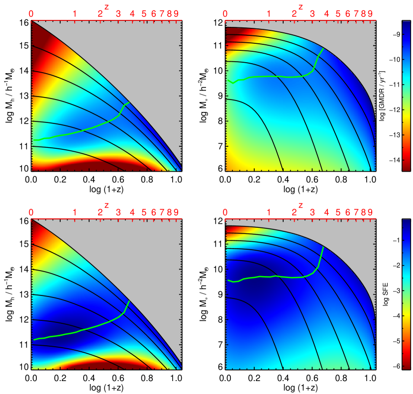
Figure 9.— Model predictions for the gas mass depletion rates (GMDR; upper panels) and star formation efficiencies (SFE; lower panels) of central galaxies as functions of halo mass (left-hand panels) or stellar mass (right-hand panels) and redshift. The color codings used are indicated in the vertical bars on the right-hand site. Whereas the SFEs are dimensionless, the GMDRs are in units of ${\rm yr}^{-1}$. As in Fig. 6, the solid, black curves show the median growth of halo mass (left-hand panel) and stellar mass (right-hand panel) along the main branch of halos with different present-day masses, while the solid, green lines mark the maximum GMDRs/SFEs as function of redshift.

5.2. Star formation rate density

Using the ‘SFR maps’ shown in the upper panels of Fig. 6, we can obtain similar maps but for the star formation rate density (SFRD). These have the advantage that they highlight when and where the majority of stars in the Universe formed. The SFRD is related to the SFRs according to

$${\rm SFRD}(M_{h},z) = \,{\rm ln}10\times n(M_{h},z)\,M_{h}$$

$$\times {\rm SFR}(M_{h},z){\frac{{\rm d}t}{{\rm d}\log(1+z)}}\,.$$

where $n(M_{h},z)\equiv{\rm d}n(z)/{\rm d}M_{h}$ is the comoving number density of halos at $z$ with masses in the range $[M_{h},M_{h}+{\rm d}M_{h}]$. Thus defined, the SFRD is the mass density of stars formed per $\log M_{h}$ per $\log(1+z)$, and the result is shown in the left-hand panel of Fig. 8. The SFRD peaks at redshift $z\sim 1$ in halos of $M_{h}\sim 10^{12}\>h^{-1}{\rm M}_{\odot}$. The solid, green contour shown on top of the SFRD map encloses the region that contributes 50% to the total SFH in the Universe, and shows that half of the total stellar mass is formed in halos with masses in the range $10^{11.1}{\>h^{-1}{\rm M}_{\odot}}\lesssim M_{h}\lesssim 10^{12.3}{\>h^{-1}{\rm M}_{\odot}}$ and in the redshift range $0.4\lesssim z\lesssim 1.9$. Overall, halos with masses $M_{h}=10^{10.5-13.5}\>h^{-1}{\rm M}_{\odot}$ contribute the vast majority of all star formation in the universe. At $z\lesssim 1.5$, the star formation density becomes progressively more dominated by low-mass halos.

A SFRD map can also be constructed in the stellar mass - redshift plane,

$${\rm SFRD}(M_{\ast},z)={\rm SFRD}(M_{h},z){\frac{{\rm d}\log M_{h}}{{\rm d}\log M_{\ast}}}\,,$$ (26)

and the results are shown in the right-hand panel of Fig. 8. Here we see that the SFRD peaks at $M_{\ast}\sim 10^{10}\>h^{-2}{\rm M}_{\odot}$, and that half of the stars in the Universe is formed in galaxies within a narrow ($\sim 1.3{\rm dex}$) stellar mass range: $10^{9.4}{\>h^{-2}{\rm M}_{\odot}}\lesssim M_{\ast}\lesssim 10^{10.7}{\>h^{-2}{\rm M}_{\odot}}$.

5.3. Star formation efficiency and gas mass depletion rate

Next we look at the gas mass depletion rates (GMDR) of central galaxies in halos of different masses. Since our current modeling does not include any gas components, we define the GMDR to be the SFR normalized by the total baryonic mass, defined as the halo mass times the universal baryon fraction $f_{b}$:

$${\rm GMDR}(M_{h},z)={{\rm SFR}(M_{h},z)\over f_{b}\,M_{h}}\,,$$ (27)

where we adopt $f_{b}\equiv\Omega_{\rm b}/\Omega_{\rm m}\simeq 0.167$ (e.g., Komatsu et al. 2011). Thus defined, the GMDR is the reciprocal of the time it takes a galaxy to consume all the gas associated with its halo at the current SFR. The top left and right panels of Fig. 9 show the GMDR maps in the halo mass vs. redshift and stellar mass vs. redshift spaces, respectively. The green solid line shown in each panel marks the maximum GMDRs as function of redshift. Three trends are worth noting. First, the GMDRs in low mass halos ($M_{h}\lesssim 10^{11}\>h^{-1}{\rm M}_{\odot}$) are always strongly suppressed with respect to their more massive counterparts. Second, at $z\gtrsim 3.5$, the most massive halos have the highest GMDRs, which are roughly constant at $\sim 10^{-9.2}\,{\rm yr}^{-1}$ over a large range in redshift. These high GMDRs result in rapid growth of the central galaxies, as is evident from the black solid lines shown in the right-hand panel. Finally, below $z\sim 3.5$ ‘downsizing’ kicks in, in that the peak in the GMDR shifts to lower halo masses with decreasing redshift. There appears to be some ‘quenching’ mechanism (or at least some mechanism that manages to strongly suppress the GMDR), which operates in halos whose mass shifts down with decreasing redshift; centrals that end up in more massive halos at $z=0$ quench at a higher redshift, when their halo mass is more massive. Whereas the present-day quenching mass is close to $10^{11}\>h^{-1}{\rm M}_{\odot}$, centrals that have ended up in the most massive halos quenched around $z\sim 3.5$ when their main progenitor halo had a mass $\sim 10^{13}\>h^{-1}{\rm M}_{\odot}$.

Figure 10.— Model predictions for the star formation efficiencies of central galaxies as function of the main branch mass, $M_{a}$, of their host halo. Results are shown for host halos with present-day masses $\log(M_{h}/\>h^{-1}{\rm M}_{\odot})=11.0,11.5,12.0$, $12.5,13.0,13.5,14.0,14.5,15.0$. The present-day mass for each curve is evident from its end-point at the high-mass end.

An insightful way of expressing the SFHs of central galaxies is to compare them with the mass accretion histories of their halos. To this end, we follow Behroozi et al. (2013) and define the star formation efficiency (SFE) of central galaxies in the main branch progenitors as

$${\rm SFE}(M_{h},z)=\frac{{\rm SFR}(M_{h},z)}{{\rm d}(f_{b}M_{a})/{\rm d}t}\,.$$ (28)

Thus defined the SFE describes the SFR in the main branch progenitor at redshift $z$ (where the halo mass is $M_{a}$) in units of the baryonic mass accretion rate at the same redshift. The lower panels of Fig. 9 show maps of the SFE in the halo mass vs. redshift (left-panel) and stellar mass vs. redshift (right-panel) spaces. The SFE peaks in halos with mass $\sim 10^{11.4}\>h^{-1}{\rm M}_{\odot}$ at redshift $\sim 0.5$, with central galaxy mass $\sim 10^{9.5}\>h^{-2}{\rm M}_{\odot}$. Compared with the GMDR maps shown in the upper panels, the peak in the SFE shifts to lower halo/stellar mass and lower redshift. This is simply a reflection of the fact that low mass halos have lower specific mass accretion rates than their more massive counterparts (i.e., more massive halos assemble later).

These results are in qualitative agreement with those obtained by Behroozi et al. (2013), but quantitatively there are differences. In particular, compared to Behroozi et al. (2013), our model seems to predict significantly stronger redshift dependence. For example, according to our model the halo mass at which the SFE is highest increases from $M_{h}\sim 10^{11.2}\>h^{-1}{\rm M}_{\odot}$ at $z=0$ to $M_{h}\sim 10^{12.1}\>h^{-1}{\rm M}_{\odot}$ at $z=3$ (see solid, green line in lower left-hand panel of Fig. 9). In contrast, the corresponding ${\rm SFE}$ peak halo masses obtained by Behroozi et al. (2013) are $10^{11.5}\>h^{-1}{\rm M}_{\odot}$ and $10^{12.0}$ at $z=0$ and $z=3$, respectively. Interestingly, we find that the stellar mass of the central galaxies for which the SFE (or GMDR) is maximal is virtually independent of redshift at $M_{\ast,c}\sim 10^{9.7}\>h^{-2}{\rm M}_{\odot}$, but only for $z\lesssim 2.5$. Our model suggests that for $z\gtrsim 2.5$, this characteristic stellar mass rapidly increases to effectively become equal to that of the most massive galaxies present at those redshifts. Such a feature is reconfirmed very recently using a different approach by Lu et al. (2013 in preparation).

To highlight some of the features of the SFEs, Fig. 10 shows cuts of the SFE maps along some of the main branch histories (solid lines in the left panels of Fig. 9). Results are shown for central galaxies with present-day halo masses of $\log(M_{h}/\>h^{-1}{\rm M}_{\odot})=11.0,11.5,12.0,12.5,13.0,13.5,14.0,14.5,15.0$. As the main progenitor mass increases with time, the SFE initially increases, reaches a maximum, after which it decreases rapidly to a quenched state. Interestingly, the initial increase of the SFE with increasing $M_{a}$ is much steeper for central galaxies that end up in less massive halos. A rapid increase of SFE over the range $10^{10}-10^{11}\>h^{-1}{\rm M}_{\odot}$ in $M_{a}$, which is predicted by our model for centrals that end-up in present-day halos with $M_{h}\lesssim 10^{12.5}\>h^{-1}{\rm M}_{\odot}$, is consistent with the presence of a ‘halo mass floor’ $M_{\rm min}\sim 10^{11}\>h^{-1}{\rm M}_{\odot}$, below which star formation is strongly suppressed, as suggested by Bouché et al (2010). However, our model predicts that central galaxies that end up in more massive halos have fairly high SFEs when their main progenitor mass is $\sim 10^{10}\>h^{-1}{\rm M}_{\odot}$. This suggests that this halo mass floor must have been substantially lower (or absent) at higher redshifts ($z\gtrsim 5$).

Another interesting feature of the SFE($M_{a}$) curves in Fig. 10 is the evolution in the ‘quenching mass’, which we define as the main-progenitor mass at which the SFE is maximal. Present-day halos with $M_{h}\gtrsim 10^{13}\>h^{-1}{\rm M}_{\odot}$ all seem to quench when $M_{a}\sim 10^{12.5}\>h^{-1}{\rm M}_{\odot}$, at which point their SFE is $\sim 0.1$ (i.e., the star formation rate is ten percent of the baryon accretion rate) . For present-day halos with $M_{h}\lesssim 10^{13}\>h^{-1}{\rm M}_{\odot}$ our model predicts a ‘downsizing’ behavior, in that the quenching mass shifts to lower $M_{a}$ for present-day halos that are less massive. In addition, the peak value of the SFE increases, coming close to unity for $M_{h}\sim 10^{11.5}\>h^{-1}{\rm M}_{\odot}$.

An important, outstanding question in galaxy formation is what physical process is responsible for the quenching of central galaxies, which seems to happen whenever the halo mass is of order $10^{12}\>h^{-1}{\rm M}_{\odot}$. Interestingly, this mass scale is very similar to the one that separates cold-mode accretion and hot-mode accretion (Birnboim & Dekel 2003; Kereš et al. 2005), suggesting that the quenching of star formation in central galaxies may be related to the ability of a dark matter halo to form a hot gaseous halo. This is indeed what seems to be needed to explain the observed bimodality in the distributions of galaxy colors and specific star formation rates (e.g., Cattaneo et al. 2006; Birnboim et al. 2007). In addition to cold mode/hot mode accretion, other mechanisms have also been invoked to explain the quenching of star formation in massive central galaxies, ranging from AGN feedback (e.g., Tabor & Binney 1993; Ciotti & Ostriker 1997; Croton et al. 2006; Bower et al. 2006; Hopkins et al. 2006) and gravitational heating (e.g., Fabian 2003; Khochfar & Ostriker 2008; Dekel & Birnboim 2008; Birnboim & Dekel 2011) to thermal conduction (e.g., Kim & Narayan 2003). Although it remains unclear which of these processes dominates, and how exactly they operate, it is clear that any successful model has to be able to explain why star formation in galaxies is quenched once their halo masses reach a characteristic mass, which ‘downsizes’ from $\sim 10^{12.5}\>h^{-1}{\rm M}_{\odot}$ at high redshifts ($z\gtrsim 3.5$) to $\sim 10^{11.5}$ at the present-day.

5.4. Comparing SFE with central-to-host halo mass ratios

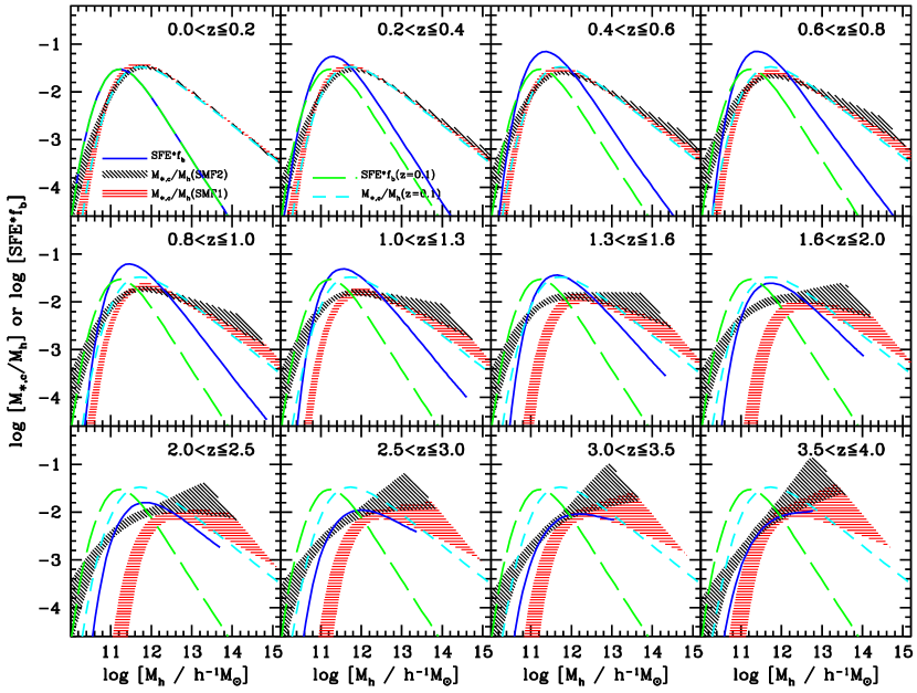
Figure 11.— Instantaneous versus integrated mass ratios. The red and black shaded regions indicate the 68% confidence levels on the ‘integrated’ mass ratios between central galaxy and host halo, $M_{\ast,c}/M_{h}$, as function of host halo mass, as obtained by Y12 from the SMF1 and SMF2 data samples, respectively. Different panels correspond to different redshift intervals, as indicated. The solid curve in each panel is the ‘instantaneous’ mass ratio, ${\rm SFE}\times f_{b}$, inferred from our model. For comparison, we also show in each panel the model predictions assuming “no-evolution”, which simply are the $M_{\ast,c}/M_{h}$ (cyan, short-dashed curves) and ${\rm SFE}\times f_{b}$ (green, long-dashed curves) at $z=0.1$.

Since the SFE indicates the fraction of newly accreted baryonic matter that is converted into stars, the quantity SFE$\times f_{b}$ can be regarded as the instantaneous mass ratio between the newly formed stars and newly accreted dark matter. It will be interesting to compare this mass ratio to that between the stellar mass of a central galaxy and the mass of its dark matter host halo. The latter has been extensively studied in recent years, and is an integration of SFE$\times f_{b}$ over cosmic time plus a contribution due to the accretion of satellite galaxies (important in massive halos at low redshift) and the impact of passive evolution (which removes $\sim 40$ percent of the stars formed at early times from the mass budget of present day stars).

We first show, in Fig. 11, the $M_{\ast,c}/M_{h}$ ratios obtained in Y12 for SMF1 (red shaded curves) and SMF2 (black shaded curves). The shaded areas reflect the 68% confidence levels resulting from the statistical errors in the resulting $M_{\ast,c}/M_{h}$ ratios. The differences between the SMF1 and SMF2 curves can be regarded as roughly reflecting the systematical errors in the current data. Compared to the ”no-evolution” model, which simply is the $M_{\ast,c}/M_{h}$ at $z=0.1$ (cyan, dashed curve in each panel), the $M_{\ast,c}/M_{h}$ ratio does evolve significantly, especially beyond redshift $z\simeq 1$. On average, the peak $M_{\ast,c}/M_{h}$ ratio at redshift $z\gtrsim 2.0$ is $\sim 0.5$dex below the one at redshift $z=0.1$.

The solid line in each panel of Fig. 11 indicates our model prediction for the instantaneous ratio, ${\rm SFE}\times f_{b}$, at the corresponding redshifts, reduced by 40% in order to (roughly) correct for passive evolution (see discussion in §3.2). Again, for comparison, we also show in each panel the “no-evolution” model predictions (long-dashed green curve), which simply is the ${\rm SFE}\times f_{b}$ ratio at $z=0.1$. Note how the peak of the ${\rm SFE}\times f_{b}$ vs. $M_{h}$ curve first increases by about $+0.4$dex from $z=0.1$ to $z\simeq 0.6$, after which it gradually decreases to about $-0.5$dex at $z\gtrsim 3.0$.

Comparing the ‘integrated’ mass ratios, $M_{\ast,c}/M_{h}$ to the ‘instantaneous’ ratios, ${\rm SFE}\times f_{b}$, in different redshift bins, one notices that the two ratios are in good agreement with each other at high redshifts ($z\gtrsim 3$). This is as expected, since (i) the SFE does not show strong time evolution at high redshift, and (ii) the contribution from satellite galaxies is negligible. Moving to lower redshifts, we see an ever increasing ‘lag’ between the ‘integrated’ and ‘instantaneous’ mass ratios at the high mass end. This is a manifestation of the quenching of central galaxies in massive haloes; their instantaneous SFRs are a poor indicator of their integrated (past) SFHs. In addition, massive centrals may have accreted a significant fraction of their stellar mass in the form of satellite galaxies (see §5.6 below), which is also not reflected in their instantaneous SFRs. Finally, at all $0.2\lesssim z\lesssim 2.5$, the peak in the ‘instantaneous’ mass ratio is higher than that in the ‘integrated’ mass ratio. This is a manifestation of the fact that the instantaneous SFE has a global peak at redshift $z\sim 0.5$. Hence, at redshifts above and in a certain range blow this peak redshift, the instantaneous mass ratio should be larger than its time-integrated equivalent.

5.5. The cosmic star formation densities

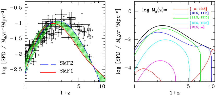
Figure 12.— The cosmic star formation densities. Left-hand panel: comparison of our model predictions with the observational data compiled by Hopkins & Beacom (2006; small dots with error bars). Our model predictions based on SMF1 and SMF2 are shown as the solid and long-dashed lines, respectively. For comparison, the shaded band indicates the range of SFDs obtained from the ‘MIN’, ‘MAX’ and ‘OBS’ models based on SMF1 and SMF2, and therefore (roughly) reflects our model uncertainties. Right-hand panel: model predictions based on SMF1 for the contributions to the total SFD due to halos of different masses, as indicated.

Once we know how the SFRs of central galaxies depend on $M_{h}$ and $z$, we can combine the dependence with the halo mass function to predict the star formation history of the universe, as described by the cosmic star formation density (SFD) defined as

$${\rm SFD}(z)=\int^{\infty}_{0}{\rm SFR}(M_{h},z)~{}n(M_{h},z){\rm d}M_{h}\,.$$ (29)

Note that our model prediction only accounts for the contribution due to central galaxies, whereas the data on the cosmic star formation history includes contributions from both centrals and satellites. However, since satellite galaxies contribute less than $\sim 40\%$ of the total galaxy population (e.g., Mandelbaum et al. 2006; Tinker et al. 2007; van den Bosch et al. 2007; Yang et al. 2008; Cacciato et al. 2013) and have significantly lower SFRs (e.g., Balogh et al. 2000; Weinmann et al. 2006, 2009; Wetzel, Tinker & Conroy 2012a,b), their contribution to the SFD is sufficiently small that a comparison of our model prediction with data is still meaningful.

In the left panel of Fig. 12, we compare our model prediction of the cosmic SFD to a compilation of data taken from Hopkins & Beacom (2006). Hopkins & Beacom (2006) converted all the SFRs to a Salpeter (1955) IMF, which is different from the Kroupa (2001) IMF used in this work. As suggested in Perez-Gonzalez et al. (2008), the stellar masses based on the Salpeter (1955) IMF are systematically larger by a factor of $\sim 1.7$ than those based on the Kroupa IMF. Here we have applied such a conversion in our comparison by multiplying our model prediction by a factor $1.7$. The solid and long dashed lines show our model predictions based on SMF1 and SMF2, respectively, with the latter obtained from the fitting formula provided in Appendix A. For comparison we also show, using a shaded band, the range of the SFDs obtained from the three models for the SFR, ‘OBS’, ‘MAX’ and ‘MIN’, and using SMF1 and SMF2. This band therefore roughly captures the uncertainties in our model.

As one can see, at low redshift ($z\lesssim 2.0$), our model prediction is in good agreement with the data. At $z\gtrsim 2.0$, however, our model under-predicts the cosmic SFD compared to the data. Several sources might contribute to this discrepancy. First, our model prediction of the SFD is based on the median SFH of central galaxies. In reality, for a given halo mass the SFR distribution has a broad (roughly log-normal) distribution (see Fig. 1). For a log-normal distribution the average SFR is larger than its median value by a factor of $e^{(\ln(10)\sigma)^{2}/2}$ which corresponds to an enhancement in the SFDs of $\sim 0.1$dex for the typical dispersion, $\sigma\sim 0.3$, shown in Fig. 1. Taking this into account will increase the predicted SFD, especially at $z=0$ because of the bi-lognormal distribution of galaxies in halos of $\sim 10^{12}\>h^{-1}{\rm M}_{\odot}$. Such an increase of $\sim 0.1$dex is insufficient to explain the apparent discrepancy at high $z$. An alternative explanation might be that we did not include the contribution due to satellite galaxies. Albeit small, adding this contribution will also slightly increase our SFD model predictions. In addition to these, the high redshift SFD depends significantly on the correction of faint galaxies. As pointed out recently by Behroozi et al. (2012) based on some new measurements of the cosmic SFD (e.g., Bouwens et al. 2012), the data compiled by Hopkins & Beacom (2006) is likely to overestimate the cosmic SFDs in the redshift range $3\lesssim z\lesssim 8$. This discrepancy is largely due to the different luminisity cuts in calculating the SFD (see Kistler et al. 2009). Taking all these uncertainties/issues into account, we conclude that our model seems to predict a cosmic SFD somewhat lower than the data at very high redshift. The discrepancy can be significantly eased either if the stellar mass functions at high redshift have a significantly steeper low mass end slope, or if the faint end slopes of the galaxy luminosity functions used in the SFD measurements are significantly under-estimated.

Finally, the right-hand panel of Fig. 12 shows our model prediction for how halos of different masses contribute to the cosmic SFD. Halos with $M_{h}<10^{10.5}\>h^{-1}{\rm M}_{\odot}$ are predicted to only contribute significantly at very high redshifts ($z\gtrsim 10$). Halos with masses $10.5<\log(M_{h}/\>h^{-1}{\rm M}_{\odot})<11.5$, on the other hand, are predicted to be the main contributors of the cosmic SFD at both $z\sim 0$ and $z\sim 7.0$. Milky-Way sized halos with masses $11.5<\log(M_{h}/\>h^{-1}{\rm M}_{\odot})<12.5$ are predicted to be the main contributors for most of the history of the Universe, all the way from $z\sim 7$ to $z\sim 0.1$. Interestingly, our model predicts that halos with $M_{h}\gtrsim 10^{12.5}\>h^{-1}{\rm M}_{\odot}$ never contributed significantly (i.e., more than 10%) to the cosmic star formation density at any redshift.

5.6. The fraction of stars formed in situ

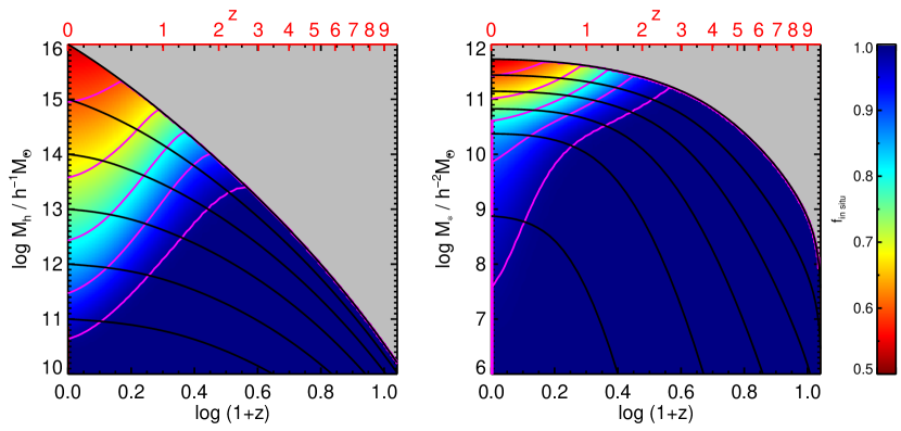
Figure 13.— Model predictions for the fraction of stars of central galaxies that formed in situ, $f_{\rm insitu}$, as function of halo mass (left-hand panel) or stellar mass (right-hand panel) and redshift. Color coding is indicated in vertical bar at the right-hand side. For clarity, the purple lines indicate the contours where $f_{\rm insitu}=0.6,0.7,0.8,0.9$ and $0.99$, respectively. The solid black curves once again show the median growth of halo mass (left-hand panel) and stellar mass (right-hand panel) along the main branch of halos with different present-day masses.

Recent cosmological simulations of galaxy formation show that the assembly of massive galaxies, which are almost always ellipticals, consists of “two phases”; a rapid early phase at $z\gtrsim 2$, during which stars are formed in situ (i.e., within the galaxy) from infalling cold gas, followed by an extended phase during which ex situ stars (in the form of satellite galaxies) are accreted (e.g. Oser et al. 2010, 2012; Hirschmann et al. 2012). Such a two-phase formation scenario for massive galaxies is supported by the strong evolution in the observed size-mass relation of massive galaxies (e.g., Bezanson et al. 2009, and references therein). Our model for the SFHs of central galaxies can predict the fraction of stars formed in situ as a function of redshift, halo mass, and stellar mass.

The total stellar mass of a central galaxy at a given redshift $z_{0}$ can be obtained from Eq. (24). The stellar mass of stars that formed in situ can be obtained by replacing ${\rm SFR}_{\rm MAX}$ by the real star formation rate ${\rm SFR}_{\rm OBS}$, so that we can write

$$M_{\ast,{\rm SF}}(z_{0})=\int_{0}^{t_{z_{0}}}{\rm SFR}_{\rm OBS}(z(t))\,f_{\rm passive}(t_{z_{0}}-t)\,{\rm d}t\,.$$ (30)

Fig. 13 shows the ratio $f_{\rm insitu}=M_{\ast,{\rm SF}}(z_{0})/M_{\ast}(z_{0})$, between the mass of stars formed in situ and the total stellar mass, in both the $M_{h}$ - $z$ (left-hand panel) and the $M_{\ast}$ - $z$ (right-hand panel) planes. We first focus on the most massive galaxies, which are typically ellipticals in massive halos. According to our model, at $z>2.5$ more than $99\%$ of the stars in these galaxies are formed in situ. This fraction decreases as a function of redshift, dropping to $\sim 60\%$ at $z=0$. Thus even today’s most massive ellipticals, for which the accretion of stars from (satellite) galaxies is expected to be most important, are predicted to have the majority of their stellar mass contributed by early, in situ star formation (on average). For central galaxies in less massive halos, the fraction of stars formed in situ is even lower. For a Milky Way sized halo of $M_{h}\sim 10^{12}\>h^{-1}{\rm M}_{\odot}$ at the present day, more than $80\%$ of the stars are expected to have formed in situ. Clearly, major mergers of stellar components (e.g. major ‘dry mergers’) of galaxies cannot be a dominant mode of stellar mass assembly for galaxies of any stellar mass (on average).

6. Summary

In this paper we have presented model predictions for the star formation histories (SFHs) of central galaxies as a function of halo mass. The model is based on self-consistent modeling of the conditional stellar mass function across cosmic time by Yang et al. (2012). Two key ingredients are used in deriving the SFHs. The first is the mass assembly histories of central galaxies and their accreted satellite galaxies, and second is the local observational constraints on the star formation rates of central galaxies as function of halo mass. The difference in total stellar mass between the accreted and surviving satellites provides the maximum contribution available to the growth of the central galaxy through accretion of stars from satellites. The minimum (zero) and maximum contributions from the accreted satellites correspond to the maximum and minimum amounts of stars that formed in situ in a central galaxy. As expected, the local observational constraints on the star formation rates (SFRs) of central galaxy, obtained from the SDSS DR7 group catalog, fall between these extrema.

Using these data, we have obtained median SFHs for central galaxies as function of their present-day halo mass. We have presented a universal fitting formula that adequately describes the dependence of these SFHs on halo mass, galaxy stellar mass and redshift. We also used this model to make predictions for (i) the star formation rates (SFRs), star formation rate densities (SFRDs), gas mass depletion rates (GMDRs), and star formation efficiencies (SFEs), all as functions of redshift, halo mass and stellar mass; (ii) the cosmic star formation rate density; and (iii) the fraction of stars that have formed in situ over cosmic time (as apposed to have been accreted). Our main findings can be summarized as follows.

1. The SSFR at high $z$ increases rapidly with increasing redshift [$\propto(1+z)^{2.5}$] for halos of a given mass, and slowly with halo mass ($\propto M_{h}^{0.12}$) for a given $z$. This scaling is almost identical to that of the specific mass accretion rate of dark matter halos (Dekel et al. 2009; McBride et al. 2009; Fakhouri et al. 2010), indicating that the SFR of (star-forming) central galaxies is largely regulated by the rate at which their host halos accrete mass. Such a picture has strong theoretical support (e.g., Dutton, van den Bosch & Dekel 2010; Bouché et al. 2010; Davé, Finlator & Oppenheimer 2012).

2. The ratio between the SFR in the halo’s main progenitor and the final stellar mass of a galaxy peaks roughly at a constant value, $\sim 10^{-9.3}h^{2}{\rm yr}^{-1}$, independent of the halo mass and stellar mass of the galaxy at the present day. The redshift at which this SFR peaks ($z_{\rm pk}$), however, increases rapidly with the present-day halo mass of the galaxy, with $z_{\rm pk}\sim 0.5$ for $M_{h}=10^{11}\>h^{-1}{\rm M}_{\odot}$, and $z_{\rm pk}\sim 3$ for $M_{h}=10^{15}\>h^{-1}{\rm M}_{\odot}$.

3. More than half of the stars in the present-day Universe were formed in halos with masses between $10^{11.1}\>h^{-1}{\rm M}_{\odot}$ and $10^{12.3}\>h^{-1}{\rm M}_{\odot}$ in the redshift range $0.4$ - $1.9$. Halos with masses between $10^{11.5}\>h^{-1}{\rm M}_{\odot}$ and $10^{12.5}\>h^{-1}{\rm M}_{\odot}$ dominate the star formation rate density of the universe over a large range of redshift, from $z\sim 1$ to $\sim 5$; at $z<1$ the star formation rate density is dominated by halos with $10^{10.5}\>h^{-1}{\rm M}_{\odot}<M_{h}<10^{11.5}\>h^{-1}{\rm M}_{\odot}$; the total amounts of stars formed in small halos with $M_{h}<10^{10.5}\>h^{-1}{\rm M}_{\odot}$ and in massive halos with $M_{h}>10^{12.5}\>h^{-1}{\rm M}_{\odot}$ are both negligibly small at any $z<5$.

4. For individual centrals, the SFE, defined as the star formation rate divided by the baryonic accretion rate, initially increases, until it reaches a maximum, after which it decreases rapidly to a quenched state. For centrals in present-day halos with $M_{h}\gtrsim 10^{13}\>h^{-1}{\rm M}_{\odot}$, quenching occurs when their main progenitor halo reaches a mass $\sim 10^{12.5}\>h^{-1}{\rm M}_{\odot}$, at which point the SFE is $\sim 0.1$. For centrals in present-day halos with $M_{h}\lesssim 10^{13}\>h^{-1}{\rm M}_{\odot}$ the quenching mass shifts to lower halo masses at higher peak SFE; at the present, the quenching mass is $\sim 2\times 10^{11}\>h^{-1}{\rm M}_{\odot}$, with a peak SFE close to unity.

5. Whereas the SFE histories of central galaxies that end-up in present-day halos with $M_{h}\lesssim 10^{12.5}\>h^{-1}{\rm M}_{\odot}$ are consistent with the presence of a halo mass floor of $\sim 10^{11}\>h^{-1}{\rm M}_{\odot}$, as suggested by Bouché et al. (2010), our model indicates that such a halo mass floor (below which star formation is suppressed) needs to be substantially lower, or even absent, at high $z$.

6. There are some indications that our model may underpredict the cosmic star formation density at high redshifts ($z\gtrsim 3$). The discrepancy can be significantly reduced if either the stellar mass functions at high redshift have a significantly steeper low-mass end slope, or the faint-end slopes of the luminosity functions used in the SFD measurements are significantly under-estimated.

7. At redshift $z\gtrsim 2.5$ more than $99\%$ of the stars in the progenitors of massive galaxies (mainly ellipticals) are formed in situ, and this fraction decreases as a function of redshift, dropping to $\sim 60\%$ at $z=0$; for a Milky Way sized halo of $M_{h}\sim 10^{12}\>h^{-1}{\rm M}_{\odot}$ more than $80\%$ of all the stars in the central galaxy are formed in situ. Hence, major mergers cannot be a dominant mode of stellar mass assembly for any stellar mass (on average).

Appendix A A. The SFH fitting formula for SMF2

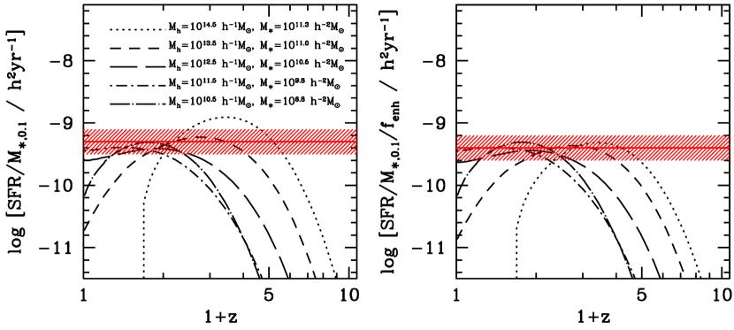
Figure 14.— Similar to right-hand panel of Fig. 4, except that here the star formation histories are obtained using SMF2, rather than SMF1. In the left-hand panel the SFHs are normalized by the stellar masses of the central galaxies at $z=0.1$, while the curves in the right-hand panel have been normalized by an additional enhancement factor, $f_{\rm enh}$, given by Eq. (A2).

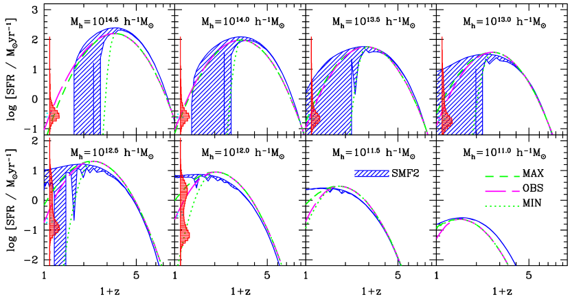
Figure 15.— The star formation histories (SFHs) of central galaxies in halos of different present-day masses, as indicated in each panel. Here we only show the results obtained from SMF2. In each panel, predictions with MIN and MAX assumptions for the star formation rate are bridged with shaded areas (see text for more details). In panels for halos with $M_{h}\geq 10^{12}\>h^{-1}{\rm M}_{\odot}$, local observational constraints are shown as the vertical shaded histograms (distributions) and stars (median). The dotted, dashed, and long-dashed lines are the MIN, MAX and OBS fits to the SFHs discussed in the text.

The discussion in the main text is mainly based on SMF1. As we have seen, the SFHs obtained from SMF1 and SMF2 have systematic differences (see, e.g., Fig. 2). For completeness, this Appendix presents our model for the SFHs of central galaxies based on SMF2, rather than SMF1. Let us first look at the amplitude of the SFHs, shown in the left panel of Fig. 14. Compared to the results obtained from SMF1 (see the right panel of Fig. 4), the peak values of the SFRs obtained from SMF2 have slightly larger variation between different halos masses. Especially the very massive galaxies in SMF2 have significantly higher SFH peaks than those in SMF1. In order to properly model the SFH peaks in the SMF2, we introduce a stellar mass dependent enhancement factor $f_{\rm enh}$, so that we can properly model the peak amplitudes. By fitting to the SFH peaks obtained from SMF2, we get the following relation between ${\rm SFR}_{\rm pk}$ and $M_{\ast,0.1}$:

$${{\rm SFR}_{\rm pk}\over[{\rm M}_{\odot}\,{\rm yr}^{-1}]}={M_{\ast,0.1}\over 10^{9.4}\>h^{-2}{\rm M}_{\odot}}f_{\rm enh}(M_{\ast,0.1})\,,$$ (A1)

where

$$f_{\rm enh}(M_{\ast,0.1})=1+(M_{\ast,0.1}/10^{11.2}\>h^{-2}{\rm M}_{\odot})^{2}\,,$$ (A2)

is a stellar mass dependent enhancement factor. The performance of the fitting results is shown in the right panel of Fig. 14. As one can see, the model describes the amplitudes remarkably well.

The shape of the SFH obtained from SMF2 can still be modeled using the same form as Eq. (18),

$${\rm SFR}(M_{h},z)={\rm SFR}_{\rm pk}\times\exp\left\{-{\log^{2}[(1+z)/(1+z_{\rm pk})]\over 2\sigma^{2}(z_{\rm pk})}\right\}\,,$$ (A3)

and here with $\sigma(z_{\rm pk})$ given as follows. For $z\geq z_{\rm pk}$,

$$\sigma(z_{\rm pk})=0.146(1+z_{\rm pk})^{-0.137}\,;$$ (A4)

while for $z<z_{\rm pk}$ it is

$$\sigma(z_{\rm pk})=\left\{\begin{array}[]{ll}0.0857(1+z_{\rm pk})^{0.391}{}{}{}&\mbox{(OBS)}\\ 0.168(1+z_{\rm pk})^{-0.208}{}{}{}&\mbox{(MAX)}\\ 0.346(1+z_{\rm pk})^{-2.18}{}{}{}&\mbox{(MIN)}\end{array}\right.\,.$$ (A8)

The predictions of this fitting model are shown as the long-dashed (OBS), dashed (MAX) and dotted (MIN) curves in Fig. 15 in comparison with the results obtained directly from SMF2.

References

- Abazajian et al. (2009) Abazajian, K. N., Adelman-McCarthy, J. K., Agüeros, M. A., et al. 2009, ApJS, 182, 543
- Avila-Reese & Firmani (2011) Avila-Reese, V., & Firmani, C. 2011, Revista Mexicana de Astronomia y Astrofisica Conference Series, 40, 27
- Balogh et al. (2000) Balogh, M. L., Navarro, J. F., & Morris, S. L. 2000, ApJ, 540, 113
- Behroozi et al. (2010) Behroozi, P. S., Conroy, C., & Wechsler, R. H. 2010, ApJ, 717, 379
- Behroozi et al. (2012) Behroozi, P. S., Wechsler, R. H., & Conroy, C. 2012, arXiv:1207.6105
- Behroozi et al. (2013) Behroozi, P. S., Wechsler, R. H., & Conroy, C. 2013, ApJ, 762, L31
- Berlind & Weinberg (2002) Berlind, A. A., & Weinberg, D. H. 2002, ApJ, 575, 587
- Bezanson et al. (2009) Bezanson, R., van Dokkum, P. G., Tal, T., Marchesini, D., Kriek, M., Franx, M., & Coppi, P. 2009, ApJ, 697, 1290
- Birnboim & Dekel (2003) Birnboim, Y., & Dekel, A. 2003, MNRAS, 345, 349
- Birnboim et al. (2007) Birnboim, Y., Dekel, A., & Neistein, E. 2007, MNRAS, 380, 339
- Birnboim & Dekel (2011) Birnboim, Y., & Dekel, A. 2011, MNRAS, 415, 2566
- Blanton et al. (2005) Blanton, M. R., Schlegel, D. J., Strauss, M. A., et al. 2005, AJ, 129, 2562
- Bouché et al. (2010) Bouché, N., et al. 2010, ApJ, 718, 1001
- Bouwens et al. (2011) Bouwens, R. J., Illingworth, G. D., Oesch, P. A., et al. 2011, ApJ, 737, 90
- Bouwens et al. (2012) Bouwens, R. J., Illingworth, G. D., Oesch, P. A., et al. 2012, ApJ, 754, 83
- Bower et al. (2007) Bower, R. G., Benson, A. J., Malbon, R., Helly, J. C., Frenk, C. S., Baugh, C. M., Cole, S., & Lacey, C. G. 2006, MNRAS, 370, 645
- Boylan-Kolchin et al. (2008) Boylan-Kolchin, M., Ma, C.-P., & Quataert, E. 2008, MNRAS, 383, 93
- Brinchmann et al. (2004) Brinchmann, J., Charlot, S., White, S. D. M., et al. 2004, MNRAS, 351, 1151
- Brown et al. (2008) Brown, M. J. I., Zheng, Z., White, M., et al. 2008, ApJ, 682, 937
- Bruzual & Charlot (2003) Bruzual, G., & Charlot, S. 2003, MNRAS, 344, 1000
- Bullock et al. (2002) Bullock, J. S., Wechsler, R. H., & Somerville, R. S. 2002, MNRAS, 329, 246
- Cacciato et al. (2009) Cacciato, M., van den Bosch, F. C., More, S., et al. 2009, MNRAS, 394, 929
- Cacciato et al. (2013) Cacciato, M., van den Bosch, F. C., More, S., Mo, H., & Yang, X. 2013, MNRAS, 430, 767
- Cattaneo et al. (2006) Cattaneo, A., Dekel, A., Devriendt, J., Guiderdoni, B., & Blaizot, J. 2006, MNRAS, 370, 1651
- Chabrier (2003) Chabrier, G. 2003, PASP, 115, 763
- Choi et al. (2010) Choi, Y.-Y., Han, D.-H., & Kim, S. S. 2010, Journal of Korean Astronomical Society, 43, 191
- Ciotti & Ostriker (1997) Ciotti, L., & Ostriker, J. P. 1997, ApJ, 487, L105
- Colless et al. (2001) Colless, M., Dalton, G., Maddox, S., et al. 2001, MNRAS, 328, 1039
- Conroy et al. (2005) Conroy, C., Newman, J. A., Davis, M., et al. 2005, ApJ, 635, 982
- Conroy et al. (2006) Conroy, C., Wechsler, R. H., & Kravtsov, A. V. 2006, ApJ, 647, 201
- Conroy et al. (2007) Conroy, C., Wechsler, R. H., & Kravtsov, A. V. 2007, ApJ, 668, 826
- Conroy & Wechsler (2009) Conroy, C., & Wechsler, R. H. 2009, ApJ, 696, 620
- Cooray (2005) Cooray, A. 2005, MNRAS, 364, 303
- Cooray (2006) Cooray, A. 2006, MNRAS, 365, 842
- Cooray & Ouchi (2006) Cooray, A., & Ouchi, M. 2006, MNRAS, 369, 1869
- Croton et al. (2006) Croton, D. J., et al. 2006, MNRAS, 365, 11
- Davé et al. (2012) Davé R., Finlator, K., & Oppenheimer, B. D. 2012, MNRAS, 421, 98
- Davis et al. (2003) Davis, M., Faber, S. M., Newman, J., et al. 2003, Proc. SPIE, 4834, 161
- Dekel & Birnboim (2008) Dekel, A., & Birnboim, Y. 2008, MNRAS, 383, 119
- Dekel et al. (2009) Dekel, A., et al. 2009, Nature, 457, 451
- Drory et al. (2005) Drory, N., Salvato, M., Gabasch, A., et al. 2005, ApJ, 619, L131
- Dutton et al. (2010) Dutton, A. A., van den Bosch, F. C., & Dekel, A. 2010, MNRAS, 405, 1690
- Fabian (2003) Fabian, A. C. 2003, MNRAS, 344, L27
- Fakhouri et al. (2010) Fakhouri, O., Ma, C.-P., & Boylan-Kolchin, M. 2010, MNRAS, 406, 2267
- Fontana et al. (2006) Fontana, A., Salimbeni, S., Grazian, A., et al. 2006, A&A, 459, 745
- Geha et al. (2012) Geha, M., Blanton, M. R., Yan, R., & Tinker, J. L. 2012, ApJ, 757, 85
- Gill et al. (2005) Gill, S. P. D., Knebe, A., & Gibson, B. K. 2005, MNRAS, 356, 1327
- Gonzalez et al. (2005) Gonzalez, A. H., Zabludoff, A. I., & Zaritsky, D. 2005, ApJ, 618, 195
- Guo et al. (2010) Guo, Q., White, S., Li, C., & Boylan-Kolchin, M. 2010, MNRAS, 404, 1111
- Hamana et al. (2006) Hamana, T., Yamada, T., Ouchi, M., Iwata, I., & Kodama, T. 2006, MNRAS, 369, 1929
- Hirschmann et al. (2012) Hirschmann, M., Naab, T., Somerville, R. S., Burkert, A., & Oser, L. 2012, MNRAS, 419, 3200
- Hopkins (2004) Hopkins, A. M. 2004, ApJ, 615, 209
- Hopkins & Beacom (2006) Hopkins, A. M., & Beacom, J. F. 2006, ApJ, 651, 142
- Hopkins et al. (2006) Hopkins, P. F., Hernquist, L., Cox, T. J., Di Matteo, T., Robertson, B., & Springel, V. 2006, ApJS, 163, 1
- Jing et al. (1998) Jing, Y. P., Mo, H. J., & Boerner, G. 1998, ApJ, 494, 1
- Kang & van den Bosch (2008) Kang, X., & van den Bosch, F. C. 2008, ApJ, 676, 101
- Keres et al. (2005) Kereš, D., Katz, N., Weinberg, D. H., & Davé, R. 2005, MNRAS, 363, 2
- Khochfar & Ostriker (2008) Khochfar, S., & Ostriker, J. P. 2008, ApJ, 680, 54
- Kim & Narayan (2003) Kim, W.-T., & Narayan, R. 2003, ApJ, 596, 889
- Kistler et al. (2009) Kistler, M. D., Yüksel, H., Beacom, J. F., Hopkins, A. M., & Wyithe, J. S. B. 2009, ApJ, 705, L104
- Komatsu et al. (2011) Komatsu, E., Smith, K. M., Dunkley, J., et al. 2011, ApJS, 192, 18
- Kroupa (2001) Kroupa, P. 2001, MNRAS, 322, 231
- Le Fèvre et al. (2005) Le Fèvre, O., Vettolani, G., Garilli, B., et al. 2005, A&A, 439, 845
- Leauthaud et al. (2012) Leauthaud, A., Tinker, J., Bundy, K., et al. 2012, ApJ, 744, 159
- Lee et al. (2006) Lee, K.-S., Giavalisco, M., Gnedin, O. Y., et al. 2006, ApJ, 642, 63
- Leitner (2012) Leitner, S. N. 2012, ApJ, 745, 149
- Leitner & Kravtsov (2011) Leitner, S. N., & Kravtsov, A. V. 2011, ApJ, 734, 48
- Lin et al. (2003) Lin, W. P., Jing, Y. P., & Lin, L. 2003, MNRAS, 344, 1327
- Ludlow et al. (2009) Ludlow, A. D., Navarro, J. F., Springel, V., et al. 2009, ApJ, 692, 931
- Mandelbaum et al. (2006) Mandelbaum, R., Seljak, U., Kauffmann, G., Hirata, C. M., & Brinkmann, J. 2006, MNRAS, 368, 715
- Marchesini et al. (2009) Marchesini, D., van Dokkum, P. G., Förster Schreiber, N. M., et al. 2009, ApJ, 701, 1765
- McBride et al. (2009) McBride, J., Fakhouri, O., & Ma, C.-P. 2009, MNRAS, 398, 1858
- Mo & Fukugita (1996) Mo, H. J., & Fukugita, M. 1996, ApJ, 467, L9
- Mo et al. (1998) Mo, H. J., Mao, S., & White, S. D. M. 1998, MNRAS, 295, 319
- Mo et al. (1999) Mo, H. J., Mao, S., & White, S. D. M. 1999, MNRAS, 304, 175
- Mo et al. (2010) Mo, H., van den Bosch, F. C., & White, S. 2010, Galaxy Formation and Evolution. Cambridge University Press, 2010. ISBN: 9780521857932,
- More et al. (2009) More, S., van den Bosch, F. C., Cacciato, M., et al. 2009, MNRAS, 392, 801
- More et al. (2011) More, S., van den Bosch, F. C., Cacciato, M., et al. 2011, MNRAS, 410, 210
- Moster et al. (2010) Moster, B. P., Somerville, R. S., Maulbetsch, C., et al. 2010, ApJ, 710, 903
- Moster et al. (2013) Moster, B. P., Naab, T., & White, S. D. M. 2013, MNRAS, 428, 3121
- Moustakas & Somerville (2002) Moustakas, L. A., & Somerville, R. S. 2002, ApJ, 577, 1
- Navarro & White (1993) Navarro, J. F., & White, S. D. M. 1993, MNRAS, 265, 271
- Neistein et al. (2011) Neistein, E., Li, C., Khochfar, S., et al. 2011, MNRAS, 416, 1486
- Neistein et al. (2011) Neistein, E., Weinmann, S. M., Li, C., & Boylan-Kolchin, M. 2011, MNRAS, 414, 1405
- Oser et al. (2010) Oser, L., Ostriker, J. P., Naab, T., Johansson, P. H., & Burkert, A. 2010, ApJ, 725, 2312
- Oser et al. (2012) Oser, L., Naab, T., Ostriker, J. P., & Johansson, P. H. 2012, ApJ, 744, 63
- Peacock & Smith (2000) Peacock, J. A., & Smith, R. E. 2000, MNRAS, 318, 1144
- Peng et al. (2012) Peng, Y., Lilly, S. J., Renzini, A., & Carollo, M. 2012, ApJ, 757, 4
- Pérez-González et al. (2008) Pérez-González, P. G., Rieke, G. H., Villar, V., et al. 2008, ApJ, 675, 234
- Purcell et al. (2008) Purcell, C. W., Bullock, J. S., & Zentner, A. R. 2008, MNRAS, 391, 550
- Salpeter (1955) Salpeter, E. E. 1955, ApJ, 121, 161
- Scannapieco et al. (2012) Scannapieco, C., Wadepuhl, M., Parry, O. H., et al. 2012, MNRAS, 423, 1726
- Seigar et al. (2007) Seigar, M. S., Graham, A. W., & Jerjen, H. 2007, MNRAS, 378, 1575
- Shankar et al. (2006) Shankar, F., Lapi, A., Salucci, P., De Zotti, G., & Danese, L. 2006, ApJ, 643, 14
- Stark et al. (2009) Stark, D. P., Ellis, R. S., Bunker, A., et al. 2009, ApJ, 697, 1493
- Tabor & Binney (1993) Tabor, G., & Binney, J. 1993, MNRAS, 263, 323
- Tinker et al. (2005) Tinker, J. L., Weinberg, D. H., Zheng, Z., & Zehavi, I. 2005, ApJ, 631, 41
- Tinker et al. (2007) Tinker, J. L., Norberg, P., Weinberg, D. H., & Warren, M. S. 2007, ApJ, 659, 877
- Tinker et al. (2008) Tinker, J., Kravtsov, A. V., Klypin, A., et al. 2008, ApJ, 688, 709
- Vale & Ostriker (2006) Vale, A., & Ostriker, J. P. 2006, MNRAS, 371, 1173
- Vale & Ostriker (2004) Vale, A., & Ostriker, J. P. 2004, MNRAS, 353, 189
- van den Bosch et al. (2003) van den Bosch, F. C., Yang, X., & Mo, H. J. 2003, MNRAS, 340, 771
- van den Bosch et al. (2007) van den Bosch, F. C., Yang, X., Mo, H. J., et al. 2007, MNRAS, 376, 841
- van den Bosch et al. (2008) van den Bosch, F. C., Aquino, D., Yang, X., Mo, H. J., Pasquali, A., McIntosh, D. H., Weinmann, S. M., & Kang, X. 2008, MNRAS, 387, 79
- Wake et al. (2011) Wake, D. A., Whitaker, K. E., Labbé, I., et al. 2011, ApJ, 728, 46
- Wang et al. (2009a) Wang, H., Mo, H. J., & Jing, Y. P. 2009a, MNRAS, 396, 2249
- Wang & Jing (2010) Wang, L., & Jing, Y. P. 2010, MNRAS, 402, 1796
- Wang et al. (2012) Wang, L., Farrah, D., Oliver, S. J., et al. 2012, arXiv:1203.5828
- Wang et al. (2009b) Wang, Y., Yang, X., Mo, H. J., et al. 2009b, ApJ, 697, 247
- Weinmann et al. (2006) Weinmann, S. M., van den Bosch, F. C., Yang, X., & Mo, H. J. 2006, MNRAS, 366, 2
- Weinmann et al. (2009) Weinmann, S. M., Kauffmann, G., van den Bosch, F. C., Pasquali, A., McIntosh, D. H., Mo, H. J., & Yang, X. 2009, MNRAS, 394, 1213
- Wetzel & White (2010) Wetzel, A. R., & White, M. 2010, MNRAS, 403, 1072
- Wetzel, Tinker & Conroy (2012) Wetzel, A. R., Tinker, J. L., & Conroy, C. 2012a, MNRAS, 424, 232
- Wetzel et al. (2012b) Wetzel, A. R., Tinker, J. L., Conroy, C., & van den Bosch, F. C. 2012b, preprint (arXiv:1206.3571)
- Wetzel et al. (2013) Wetzel, A. R., Tinker, J. L., Conroy, C., & van den Bosch, F. C. 2013, in preparation
- White et al. (2007) White, M., Zheng, Z., Brown, M. J. I., Dey, A., & Jannuzi, B. T. 2007, ApJ, 655, L69
- Wolf et al. (2004) Wolf, C., Meisenheimer, K., Kleinheinrich, M., et al. 2004, A&A, 421, 913
- Yan et al. (2003) Yan, R., Madgwick, D. S., & White, M. 2003, ApJ, 598, 848
- Yang et al. (2003) Yang, X., Mo, H. J., & van den Bosch, F. C. 2003, MNRAS, 339, 1057
- Yang et al. (2005) Yang, X., Mo, H. J., van den Bosch, F. C., & Jing, Y. P. 2005, MNRAS, 356, 1293
- Yang et al. (2007) Yang, X., Mo, H. J., van den Bosch, F. C., et al. 2007, ApJ, 671, 153
- Yang et al. (2008) Yang, X., Mo, H. J., & van den Bosch, F. C. 2008, ApJ, 676, 248
- Yang et al. (2009) Yang, X., Mo, H. J., & van den Bosch, F. C. 2009a, ApJ, 693, 830
- Yang et al. (2009) Yang, X., Mo, H. J., & van den Bosch, F. C. 2009b, ApJ, 695, 900
- Yang et al. (2011) Yang, X., Mo, H. J., Zhang, Y., & van den Bosch, F. C. 2011, ApJ, 741, 13
- Yang et al. (2012) Yang, X., Mo, H. J., van den Bosch, F. C., Zhang, Y., & Han, J. 2012, ApJ, 752, 41
- York et al. (2000) York, D. G., Adelman, J., Anderson, J. E., Jr., et al. 2000, AJ, 120, 1579
- Zentner et al. (2005) Zentner, A. R., Berlind, A. A., Bullock, J. S., Kravtsov, A. V., & Wechsler, R. H. 2005, ApJ, 624, 505
- Zhao et al. (2003) Zhao, D. H., Mo, H. J., Jing, Y. P., Börner, G. 2003, MNRAS, 339, 12
- Zhao et al. (2009) Zhao, D. H., Jing, Y. P., Mo, H. J., Börner, G. 2009, ApJ, 707, 354
- Zheng (2004) Zheng, Z. 2004, ApJ, 610, 61
- Zheng et al. (2005) Zheng, Z., Berlind, A. A., Weinberg, D. H., et al. 2005, ApJ, 633, 791
- Zheng et al. (2007) Zheng, Z., Coil, A. L., & Zehavi, I. 2007, ApJ, 667, 760
- Zhu et al. (2011) Zhu, W., Feng, L.-L., & Fang, L.-Z. 2011, MNRAS, 415, 1093