A Comparison of Superposition Coding Schemes

Abstract

There are two variants of superposition coding schemes. Cover’s original superposition coding scheme has code clouds of the identical shape, while Bergmans’s superposition coding scheme has code clouds of independently generated shapes. These two schemes yield identical achievable rate regions in several scenarios, such as the capacity region for degraded broadcast channels. This paper shows that under the optimal maximum likelihood decoding, these two superposition coding schemes can result in different rate regions. In particular, it is shown that for the two-receiver broadcast channel, Cover’s superposition coding scheme can achieve rates strictly larger than Bergmans’s scheme.

I Introduction

Superposition coding is one of the fundamental building blocks of coding schemes in network information theory. This idea was first introduced by Cover in 1970 at the IEEE International Symposium on Information Theory, Noordwijk, the Netherlands, in a talk titled “Simultaneous Communication,” and appeared in his 1972 paper [6]. Subsequently, Bergmans [2] adapted Cover’s superposition coding scheme to the general degraded broadcast channel (this scheme is actually applicable to any nondegraded broadcast channel), which establishes the capacity region along with the converse proof by Gallager [11]. Since then, superposition coding has been applied in numerous problems, including multiple access channels [12], interference channels [3, 13, 5], relay channels [7], channels with feedback [8, 15], and wiretap channels [9, 4].

In a nutshell, the objective of superposition coding is to communicate two message simultaneously by encoding them into a single signal in two layers. A “better” receiver of the signal can then recover the messages on both layers while a “worse” receiver can recover the message on the coarse layer of the signal and ignore the one on the fine layer.

On a closer look, there are two variants of the superposition coding idea in the literature, which differ in how the codebooks are generated. The first variant is described in Cover’s original 1972 paper [6]. Both messages are first encoded independently via separate random codebooks of auxiliary sequences. To send a message pair, the auxiliary sequences associated with each message are then mapped through a symbol-by-symbol superposition function (such as addition) to generate the actual codeword. One can visualize the image of one of the codebooks centered around a fixed codeword from the other as a “cloud” (see the illustration in Figure 1(a)). Since all clouds are images of the same random codebook (around different cloud centers), we refer to this variant as homogeneous superposition coding. Note that in this variant, both messages enter on an equal footing and the corresponding auxiliary sequences play the same role. Thus, there is no natural distinction between “coarse” and “fine” layers and there are two ways to group the resulting superposition codebook into clouds.

The second variant was introduced in Bergmans’s 1973 paper [2]. Here, the coarse message is encoded in a random codebook of auxiliary sequences. For each auxiliary sequence, a random satellite codebook is generated conditionally independently to represent the fine layer message. This naturally results in clouds of codewords given each such satellite codebook. Since all clouds are generated independently, we refer to this variant as heterogeneous superposition coding. This is illustrated in Figure 1(b).

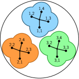
(a) Homogeneous coding

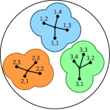
(b) Heterogeneous coding

Figure 1: Superposition codebooks for which (a) the structure within each cloud is identical and (b) the structure is nonidentical between clouds. Codewords (dots) are annotated by “$m_{1},m_{2}$”, where $m_{1}$ is the coarse layer message and $m_{2}$ is the fine layer message.

A natural question is whether these two variants are fundamentally different, and if so, which of the two is preferable. Both variants achieve the capacity region of the degraded broadcast channel [2]. For the two-user-pair interference channel, the two variants again achieve the identical Han–Kobayashi inner bound (see [13] for homogeneous superposition coding and [5] for heterogeneous superposition coding). Since heterogeneous superposition coding usually yields a simpler characterization of the achievable rate region with fewer auxiliary random variables, it is tempting to prefer this variant.

In contrast, we show in this paper that homogeneous superposition coding always achieves a rate region at least as large as that of heterogeneous superposition coding for two-user broadcast channels, provided that the optimal maximum likelihood decoding rule is used. Furthermore, this dominance can be sometimes strict. Intuitively speaking, homogeneous superposition coding results in more structured interference from the undesired layer, the effect of which becomes tangible under optimal decoding.

The rest of the paper is as follows. In Section II, we formally define the two variants of superposition coding schemes and present their respective rate regions. In Section III, we compare these rate regions. Additional remarks are provided in Section IV.

Throughout the paper, we closely follow the notation in [10]. In particular, for $X\sim p(x)$ and $\epsilon\in(0,1)$, we define the set of $\epsilon$-typical $n$-sequences $x^{n}$ (or the typical set in short) [14] as ${\mathcal{T}_{\epsilon}^{(n)}}(X)=\{x^{n}\mathchar 58\relax\mathchoice{\mspace{1.0mu}|\mspace{1.0mu}}{|}{|}{|}\#\{i\mathchar 58\relax x_{i}=x\}/n-p(x)\mathchoice{\mspace{1.0mu}|\mspace{1.0mu}}{|}{|}{|}\leq\epsilon p(x)\text{ for all }x\in\mathcal{X}\}$.

II Rate Regions for the Two-Receiver BC

Consider a two-receiver discrete memoryless broadcast channel depicted in Figure 2. The sender wishes to communicate message $M_{1}$ to receiver 1 and message $M_{2}$ to receiver 2. We define a $(2^{nR_{1}},2^{nR_{2}},n)$ code by an encoder $x^{n}(m_{1},m_{2})$ and two receivers ${\hat{m}}_{1}(y_{1}^{n})$ and ${\hat{m}}_{2}(y_{2}^{n})$. We assume the message pair $(M_{1},M_{2})$ is uniform over $[1\mathchoice{\mspace{-1.5mu}\mathchar 58\relax\mspace{-1.5mu}}{\mspace{-1.5mu}\mathchar 58\relax\mspace{-1.5mu}}{\mathchar 58\relax}{\mathchar 58\relax}2^{nR_{1}}]\times[1\mathchoice{\mspace{-1.5mu}\mathchar 58\relax\mspace{-1.5mu}}{\mspace{-1.5mu}\mathchar 58\relax\mspace{-1.5mu}}{\mathchar 58\relax}{\mathchar 58\relax}2^{nR_{2}}]$ and independent of each other. The average probability of error is defined as ${P_{e}^{(n)}}=\operatorname{\textsf{P}}\{(M_{1},M_{2})\neq(\hat{M}_{1},\hat{M}_{2})\}$. A rate pair $(R_{1},R_{2})$ is said to be achievable if there exists a sequence of $(2^{nR_{1}},2^{nR_{2}},n)$ code such that $\lim_{n\to\infty}{P_{e}^{(n)}}=0$.

\psfrag{m}[c]{\footnotesize$M_{1},M_{2}$}\psfrag{x}[b]{\footnotesize$X^{n}$}\psfrag{p}[c]{\footnotesize$p(y_{1},y_{2}\mathchoice{\mspace{1.0mu}|\mspace{1.0mu}}{|}{|}{|}x)$}\psfrag{y1}[b]{\footnotesize$Y_{1}^{n}$}\psfrag{y2}[b]{\footnotesize$Y_{2}^{n}$}\psfrag{m1}[b]{\footnotesize${\hat{M}}_{1}$}\psfrag{m2}[b]{\footnotesize${\hat{M}}_{2}$}\psfrag{e}[c]{\footnotesize Enc}\psfrag{d1}[c]{\footnotesize Dec~{}1}\psfrag{d2}[c]{\footnotesize Dec~{}2}\includegraphics[scale={0.4}]{figs/broadcast.eps}

Figure 2: Two-receiver broadcast channel.

We now describe the two superposition coding techniques for this channel and compare their achievable rate regions under optimal decoding.

II-A Homogeneous Superposition Coding ($UV$ Scheme)

Codebook generation: Fix a pmf $p(u)\hskip 1.50696ptp(v)$ and a function $x(u,v)$. Randomly and independently generate $2^{nR_{1}}$ sequences $u^{n}(m_{1})$, $m_{1}\in[1\mathchoice{\mspace{-1.5mu}\mathchar 58\relax\mspace{-1.5mu}}{\mspace{-1.5mu}\mathchar 58\relax\mspace{-1.5mu}}{\mathchar 58\relax}{\mathchar 58\relax}2^{nR_{1}}]$, each according to $\prod_{i=1}^{n}p_{U}(u_{i})$, and $2^{nR_{2}}$ sequences $v^{n}(m_{2})$, $m_{2}\in[1\mathchoice{\mspace{-1.5mu}\mathchar 58\relax\mspace{-1.5mu}}{\mspace{-1.5mu}\mathchar 58\relax\mspace{-1.5mu}}{\mathchar 58\relax}{\mathchar 58\relax}2^{nR_{2}}]$, each according to $\prod_{i=1}^{n}p_{V}(v_{i})$.

Encoding: To send the message pair $(m_{1},m_{2})$, transmit $x_{i}(u_{i}(m_{1}),v_{i}(m_{2}))$ at time $i\in[1\mathchoice{\mspace{-1.5mu}\mathchar 58\relax\mspace{-1.5mu}}{\mspace{-1.5mu}\mathchar 58\relax\mspace{-1.5mu}}{\mathchar 58\relax}{\mathchar 58\relax}n]$.

Decoding: Both receivers use simultaneous nonunique decoding, which is rate-optimal in the sense that it achieves the same rate region as maximum likelihood decoding [1] under the codebook ensemble at hand. In particular, upon receiving $y_{1}^{n}$, receiver 1 declares ${\hat{m}}_{1}$ is sent if it is the unique message such that

$$\big{(}u^{n}({\hat{m}}_{1}),v^{n}(m_{2}),y_{1}^{n}\big{)}\in{\mathcal{T}_{\epsilon}^{(n)}}$$

for some $m_{2}$. If there is no unique  ${\hat{m}}_{1}$, it declares an error. Similarly, upon receiving $y_{2}^{n}$, receiver 2 declares ${\hat{m}}_{2}$ is sent if it is the unique message such that

$$\big{(}u^{n}(m_{1}),v^{n}({\hat{m}}_{2}),y_{2}^{n}\big{)}\in{\mathcal{T}_{\epsilon}^{(n)}}$$

for some $m_{1}$. If there is no unique ${\hat{m}}_{2}$, it declares an error. Standard typicality arguments show that receiver 1 will succeed if

$$R_{1}<I(U;Y_{1})\quad\quad\text{or}\qquad\begin{aligned} R_{1}+R_{2}&<I(X;Y_{1})\\ R_{1}&<I(X;Y_{1}\mathchoice{\,|\,}{\mspace{2.0mu}|\mspace{2.0mu}}{|}{|}V),\end{aligned}$$ (1)

or, equivalently, if

$$R_{1} <I(X;Y_{1}\mathchoice{\,|\,}{\mspace{2.0mu}|\mspace{2.0mu}}{|}{|}V)$$

$$R_{1}+\min\{R_{2},I(X;Y_{1}\mathchoice{\,|\,}{\mspace{2.0mu}|\mspace{2.0mu}}{|}{|}U)\} <I(X;Y_{1}).$$

Similarly, receiver 2 will succeed if

$$R_{2}<I(V;Y_{2})\quad\quad\text{or}\qquad\begin{aligned} R_{1}+R_{2}&<I(X;Y_{2})\\ R_{2}&<I(X;Y_{2}\mathchoice{\,|\,}{\mspace{2.0mu}|\mspace{2.0mu}}{|}{|}U),\end{aligned}$$ (2)

or, equivalently, if

$$R_{2} <I(X;Y_{2}\mathchoice{\,|\,}{\mspace{2.0mu}|\mspace{2.0mu}}{|}{|}U)$$

$$R_{2}+\min\{R_{1},I(X;Y_{2}\mathchoice{\,|\,}{\mspace{2.0mu}|\mspace{2.0mu}}{|}{|}V)\} <I(X;Y_{2}).$$

The regions for both receivers are depicted in Table II-A. Letting $\mathscr{R}_{UV}(p)$ denote the set of rates $(R_{1},R_{2})$ satisfying (1) and (2), it follows that the rate region

$$\mathscr{R}_{UV}=\text{co}\bigg{(}\bigcup_{p\in\mathcal{P}_{UV}}\mathscr{R}_{UV}(p)\bigg{)}$$

is achievable. Here, $\text{co}(\cdot)$ denotes convex hull, and $\mathcal{P}_{UV}$ is the set of distributions of the form $p=p(u)\hskip 1.50696ptp(v)\hskip 1.50696ptp(x\mathchoice{\mspace{1.0mu}|\mspace{1.0mu}}{|}{|}{|}u,v)$ where $p(x\mathchoice{\mspace{1.0mu}|\mspace{1.0mu}}{|}{|}{|}u,v)$ represents a deterministic function.

	Receiver 1	Receiver 2
$\mathscr{R}_{UV}(p)$	$\hskip 118.0002ptR_{1}<I(X;Y_{1}\mathchoice{\,|\,}{\mspace{2.0mu}|\mspace{2.0mu}}{|}{|}V)$	$\hskip 118.0002ptR_{2}<I(X;Y_{2}\mathchoice{\,|\,}{\mspace{2.0mu}|\mspace{2.0mu}}{|}{|}U)$
$p=p(u)\hskip 1.50696ptp(v)\hskip 1.50696ptp(x\mathchoice{\mspace{1.0mu}|\mspace{1.0mu}}{|}{|}{|}u,v)$	$R_{1}+\min\{R_{2},I(X;Y_{1}\mathchoice{\,|\,}{\mspace{2.0mu}|\mspace{2.0mu}}{|}{|}U)\}<I(X;Y_{1})$	$R_{2}+\min\{R_{1},I(X;Y_{2}\mathchoice{\,|\,}{\mspace{2.0mu}|\mspace{2.0mu}}{|}{|}V)\}<I(X;Y_{2})$

& $\mathscr{R}_{UX}(p)$ $R_{1}+\min\{R_{2},I(X;Y_{1}\mathchoice{\,|\,}{\mspace{2.0mu}|\mspace{2.0mu}}{|}{|}U)\}<I(X;Y_{1})$ $\hskip 37.00002ptR_{2}<I(X;Y_{2}\mathchoice{\,|\,}{\mspace{2.0mu}|\mspace{2.0mu}}{|}{|}U)$ $p=p(u,x)$ $R_{1}+R_{2}<I(X;Y_{2})$

TABLE I: Rate regions for homogeneous and heterogeneous superposition coding.

II-B Heterogeneous Superposition Coding (UX Scheme)

Codebook generation: Fix a pmf $p(u,x)$. Randomly and independently generate $2^{nR_{1}}$ sequences $u^{n}(m_{1})$, $m_{1}\in[1\mathchoice{\mspace{-1.5mu}\mathchar 58\relax\mspace{-1.5mu}}{\mspace{-1.5mu}\mathchar 58\relax\mspace{-1.5mu}}{\mathchar 58\relax}{\mathchar 58\relax}2^{nR_{1}}]$, each according to $\prod_{i=1}^{n}p_{U}(u_{i})$. For each message $m_{1}\in[1\mathchoice{\mspace{-1.5mu}\mathchar 58\relax\mspace{-1.5mu}}{\mspace{-1.5mu}\mathchar 58\relax\mspace{-1.5mu}}{\mathchar 58\relax}{\mathchar 58\relax}2^{nR_{1}}]$, randomly and conditionally independently generate $2^{nR_{2}}$ sequences $x^{n}(m_{1},m_{2})$, $m_{2}\in[1\mathchoice{\mspace{-1.5mu}\mathchar 58\relax\mspace{-1.5mu}}{\mspace{-1.5mu}\mathchar 58\relax\mspace{-1.5mu}}{\mathchar 58\relax}{\mathchar 58\relax}2^{nR_{2}}]$, each according to $\prod_{i=1}^{n}p_{X\mathchoice{\mspace{1.0mu}|\mspace{1.0mu}}{|}{|}{|}U}(x_{i}\mathchoice{\mspace{1.0mu}|\mspace{1.0mu}}{|}{|}{|}u_{i}(m_{1}))$.

Encoding: To send $(m_{1},m_{2})$, transmit $x^{n}(m_{1},m_{2})$.

Decoding: Both receivers use simultaneous nonunique decoding, which is rate-optimal as we show below. In particular, upon receiving $y_{1}^{n}$, receiver 1 declares ${\hat{m}}_{1}$ is sent if it is the unique message such that (u^n(^m_1),x^n(^m_1,m_2),y_1^n ) ∈T_ϵ^(n) for some $m_{2}$. If there is no unique ${\hat{m}}_{1}$, it declares an error. Similarly, upon receiving $y_{2}^{n}$, receiver 2 declares ${\hat{m}}_{2}$ is sent if it is the unique message such that (u^n(m_1),x^n(m_1,^m_2),y_2^n ) ∈T_ϵ^(n) for some $m_{1}$. If there is no unique ${\hat{m}}_{2}$, it declares an error. Standard arguments show that receiver 1 will succeed if

$$R_{1}<I(U;Y_{1})\qquad\text{or}\qquad R_{1}+R_{2}<I(X;Y_{1}),$$ (3)

or, equivalently, if

$$R_{1}+\min\{R_{2},I(X;Y_{1}\mathchoice{\,|\,}{\mspace{2.0mu}|\mspace{2.0mu}}{|}{|}U)\}<I(X;Y_{1}).$$

Following an analogous argument to the one in [1], it can be shown that this region cannot be improved by applying maximum likelihood decoding.

Receiver 2 will succeed if

$$\begin{split}R_{2}&\leq I(X;Y_{2}\mathchoice{\,|\,}{\mspace{2.0mu}|\mspace{2.0mu}}{|}{|}U)\\ R_{1}+R_{2}&\leq I(X;Y_{2}).\end{split}$$ (4)

In the Appendix, we show that this region cannot be improved by applying maximum likelihood decoding. The regions for both receivers are depicted in Table II-A. Let $\mathscr{R}_{UX}(p)$ denote the set of all $(R_{1},R_{2})$ pairs satisfying both (3) and (4). Clearly, the rate region R_UX=co(⋃_p∈P_UX R_UX(p)) is achievable. Here, $\mathcal{P}_{UX}$ is the set of distributions of the form $p=p(u,x)$.

If the roles of $m_{1}$ and $m_{2}$ in code generation are reversed, one can also achieve the region $\mathscr{R}_{VX}=\text{co}(\cup_{p}\mathscr{R}_{VX}(p))$ obtained by swapping $Y_{1}$ with $Y_{2}$ and $R_{1}$ with $R_{2}$ in the definition of $\mathscr{R}_{UX}(p)$.

It is worth reiterating that the two schemes above differ only in the dependence/independence between clouds around different $u^{n}$ sequences, and not in the underlying distributions from which the clouds are generated. Indeed, it is well known that the classes of distributions $\mathcal{P}_{UX}$ and $\mathcal{P}_{UV}$ are equivalent in the sense that for every $p(u,x)\in\mathcal{P}_{UX}$, there exists a $q(u)\hskip 1.50696ptq(v)\hskip 1.50696ptq(x\mathchoice{\mspace{1.0mu}|\mspace{1.0mu}}{|}{|}{|}u,v)\in\mathcal{P}_{UV}$ such that $\sum_{v}q(u)\hskip 1.50696ptq(v)\hskip 1.50696ptq(x\mathchoice{\mspace{1.0mu}|\mspace{1.0mu}}{|}{|}{|}u,v)=p(u,x)$ (see for example [10, p. 626]).

III Main Result

Theorem 1.

The rate region achieved by homogeneous superposition coding includes the rate region achieved by heterogeneous superposition coding, i.e.,

$$\text{co}\big{(}\mathscr{R}_{UX}\cup\mathscr{R}_{VX}\big{)} \subseteq\mathscr{R}_{UV}.$$

Moreover, there are channels for which the inclusion is strict.

(a) Rate region in (6).

(b) Rate region in (7).

Figure 3: Rate regions for the proof of Theorem 1.

Proof.

Due to the convexity of $\mathscr{R}_{UV}$ and the symmetry between $UX$ and $VX$ coding, it suffices to show that $\mathscr{R}_{UX}(p)\subseteq\mathscr{R}_{UV}$ for all $p\in\mathcal{P}_{UX}$. Fix any $p\in\mathcal{P}_{UX}$. Let $q^{\prime}\in\mathcal{P}_{UV}$ be such that $U=X$, $V=\emptyset$, and the marginal on $X$ is preserved $q^{\prime}(x)=p(x)$. Let $q^{\prime\prime}\in\mathcal{P}_{UV}$ be such that $V=X,U=\emptyset$, and the marginal on $X$ is preserved $q^{\prime\prime}(x)=p(x)$. An inspection of (1)–(4) and Table II-A reveals that $\mathscr{R}_{UV}(q^{\prime})$ is the set of rates satisfying

$$R_{2} =0$$

$$R_{1} \leq I(X;Y_{1}),$$

and $\mathscr{R}_{UV}(q^{\prime\prime})$ is the set of rates satisfying

$$R_{1} =0$$

$$R_{2} \leq I(X;Y_{2}).$$

It then follows that $\text{co}\big{(}\mathscr{R}_{UV}(q^{\prime})\cup\mathscr{R}_{UV}(q^{\prime\prime})\big{)}$ includes the rate region

$$R_{1}+R_{2}\leq\min\big{\{}I(X;Y_{1}),I(X;Y_{2})\big{\}}.$$ (5)

We will consider three cases and show the claim for each.

• If $I(X;Y_{1})\geq I(X;Y_{2})$ then $\mathscr{R}_{UX}(p)$ reduces to the rate region

  $$R_{2} \leq I(X;Y_{2}\mathchoice{\,|\,}{\mspace{2.0mu}|\mspace{2.0mu}}{|}{|}U)$$

  $$R_{1}+R_{2} \leq I(X;Y_{2}),$$

  which is included in the rate region in (5), and therefore in $\mathscr{R}_{UV}$.

• If $I(X;Y_{1})<I(X;Y_{2})$ and $I(X;Y_{1}\mathchoice{\,|\,}{\mspace{2.0mu}|\mspace{2.0mu}}{|}{|}U)\geq I(X;Y_{2}\mathchoice{\,|\,}{\mspace{2.0mu}|\mspace{2.0mu}}{|}{|}U)$, then $\mathscr{R}_{UX}(p)$ reduces to the rate region

  $$R_{2} \leq I(X;Y_{2}\mathchoice{\,|\,}{\mspace{2.0mu}|\mspace{2.0mu}}{|}{|}U)$$

  $$R_{1}+R_{2} \leq I(X;Y_{1}),$$

  which is also included in the rate region in (5), and therefore in $\mathscr{R}_{UV}$.

• If $I(X;Y_{1})<I(X;Y_{2})$ and $I(X;Y_{1}\mathchoice{\,|\,}{\mspace{2.0mu}|\mspace{2.0mu}}{|}{|}U)<I(X;Y_{2}\mathchoice{\,|\,}{\mspace{2.0mu}|\mspace{2.0mu}}{|}{|}U)$, then $\mathscr{R}_{UX}(p)$ reduces to the rate region (see Figure 3(a))

  $$\begin{split}R_{2}&\leq I(X;Y_{2}\mathchoice{\,|\,}{\mspace{2.0mu}|\mspace{2.0mu}}{|}{|}U)\\ R_{1}+\min\{R_{2},I(X;Y_{1}\mathchoice{\,|\,}{\mspace{2.0mu}|\mspace{2.0mu}}{|}{|}U)\}&\leq I(X;Y_{1}).\end{split}$$ (6)

  Find a $q\in\mathcal{P}_{UV}$ with $q(u,x)=p(u,x)$, and note that $\mathscr{R}_{UV}(q)$ is described by the bounds

  $$\begin{split}R_{2}&\leq I(X;Y_{2}\mathchoice{\,|\,}{\mspace{2.0mu}|\mspace{2.0mu}}{|}{|}U)\\ R_{1}&\leq I(X;Y_{1}\mathchoice{\,|\,}{\mspace{2.0mu}|\mspace{2.0mu}}{|}{|}V)\\ R_{1}+\min\{R_{2},I(X;Y_{1}\mathchoice{\,|\,}{\mspace{2.0mu}|\mspace{2.0mu}}{|}{|}U)\}&\leq I(X;Y_{1}).\end{split}$$ (7)

  Comparing (6) with (7) (Figure 3(b)), one sees that $\mathscr{R}_{UX}(p)\subseteq\text{co}\big{(}\mathscr{R}_{UV}(q)\cup\mathscr{R}_{UV}(q^{\prime})\big{)}$. This proves the first claim of the theorem.

Now consider the vector broadcast channel with binary inputs $(X_{1},X_{2})$ and outputs $(Y_{1},Y_{2})=(X_{1},X_{2})$. For all $p\in\mathcal{P}_{UX}$, we have from (4) that $R_{1}+R_{2}\leq I(X_{1}X_{2};Y_{2})\leq 1$, and similarly for all $p\in\mathcal{P}_{VX}$. Thus, $\big{(}\mathscr{R}_{UX}\cup\mathscr{R}_{VX}\big{)}$ is included in the rate region $R_{1}+R_{2}\leq 1$. Note, however, that the rate pair $(1,1)$ is achievable using the $UV$ scheme by setting $U=X_{1}$ and $V=X_{2}$. This proves the second claim. ∎

IV Discussion

In addition to the basic superposition coding schemes presented in Section II, one can consider coded time sharing [10], which could potentially enlarge the achievable rate regions. In the present setting, however, it can be easily checked that coded time sharing does not enlarge $\mathscr{R}_{UX}$. Thus, the conclusion of Theorem 1 continues to hold and homogeneous superposition coding with coded time sharing outperforms heterogeneous superposition coding with coded time sharing.

[Optimality of the Rate Region in (4)] We show that no decoding rule for receiver 2 can achieve a larger rate region than the one in (4) given the codebook ensemble of heterogeneous superposition coding. To this end, denote the random codebook by C= (U^n(1),U^n(2),…, X^n(1,1), X^n(1,2), …). By the averaged version of Fano’s inequality in [1],

$$H(M_{2}\mathchoice{\,|\,}{\mspace{2.0mu}|\mspace{2.0mu}}{|}{|}Y_{2}^{n},\mathcal{C}) \leq n\epsilon_{n},$$ (8)

where $\epsilon_{n}\to 0$ as $n\to\infty$. Thus,

$$nR_{2} =H(M_{2})$$

$$\leq I(M_{2};Y_{2}^{n}\mathchoice{\,|\,}{\mspace{2.0mu}|\mspace{2.0mu}}{|}{|}\mathcal{C})+n\epsilon_{n}$$

$$\overset{\text{(a)}}{=}I(M_{2};Y_{2}^{n}\mathchoice{\,|\,}{\mspace{2.0mu}|\mspace{2.0mu}}{|}{|}\mathcal{C},M_{1})+n\epsilon_{n}$$

$$=H(Y_{2}^{n}\mathchoice{\,|\,}{\mspace{2.0mu}|\mspace{2.0mu}}{|}{|}\mathcal{C},M_{1})-H(Y_{2}^{n}\mathchoice{\,|\,}{\mspace{2.0mu}|\mspace{2.0mu}}{|}{|}\mathcal{C},M_{1},M_{2})+n\epsilon_{n}$$

$$\overset{\text{\!\!\!(b)\!\!\!}}{\leq}nH(Y_{2}\mathchoice{\,|\,}{\mspace{2.0mu}|\mspace{2.0mu}}{|}{|}U)-H(Y_{2}\mathchoice{\,|\,}{\mspace{2.0mu}|\mspace{2.0mu}}{|}{|}X)+n\epsilon_{n}$$

$$=I(X;Y_{2}\mathchoice{\,|\,}{\mspace{2.0mu}|\mspace{2.0mu}}{|}{|}U)+n\epsilon_{n},$$

where (a) follows by providing $M_{1}$ to receiver 2 as side information from a genie and (b) follows from the codebook ensemble and the memoryless property.

To see the second inequality, first assume that

$$R_{1}<I(X;Y_{2}).$$ (9)

After receiver 2 has recovered $m_{2}$, the codebook given this message reduces to C’ = (X^n(1,m_2), X^n(2,m_2), X^n(3,m_2),…). These codewords are pairwise independent since they do not share common $U^{n}$ sequences, and thus $\mathcal{C}^{\prime}$ is a nonlayered random codebook. Since (9) holds, receiver 2 can reliably recover $M_{1}$ by using, for example, a typicality decoder. Thus, by (8),

$$H(M_{1},M_{2}\mathchoice{\,|\,}{\mspace{2.0mu}|\mspace{2.0mu}}{|}{|}Y_{2}^{n},\mathcal{C}) =H(M_{2}\mathchoice{\,|\,}{\mspace{2.0mu}|\mspace{2.0mu}}{|}{|}Y_{2}^{n},\mathcal{C})+H(M_{1}\mathchoice{\,|\,}{\mspace{2.0mu}|\mspace{2.0mu}}{|}{|}Y_{2}^{n},\mathcal{C},M_{2})$$

$$\leq 2n\epsilon_{n}.$$

Hence

$$n(R_{1}+R_{2}) =H(M_{1},M_{2})$$

$$\leq I(M_{1},M_{2};Y_{2}^{n}\mathchoice{\,|\,}{\mspace{2.0mu}|\mspace{2.0mu}}{|}{|}\mathcal{C})+2n\epsilon_{n}$$

$$\leq nI(X;Y_{2})+2n\epsilon_{n}.$$ (10)

To conclude the argument, assume there exists a decoding rule that achieves a rate point $(R_{1},R_{2})$ with $R_{1}\geq I(X;Y_{2})$. Then, this decoding rule must also achieve $(R^{\prime}_{1},R^{\prime}_{2})=(I(X;Y_{2})-R_{2}/2,R_{2})$, a rate point that is dominated by $(R_{1},R_{2})$. Since $R^{\prime}_{1}<I(X;Y_{2})$, by our previous argument, $(R^{\prime}_{1},R^{\prime}_{2})$ must satisfy (10). It does not, which yields a contradiction.

References

• [1] B. Bandemer, A. El Gamal, and Y.-H. Kim, “Optimal achievable rates for interference networks with random codes,” 2012, preprint available at http://arxiv.org/abs/1210.4596/.
• [2] P. P. Bergmans, “Random coding theorem for broadcast channels with degraded components,” IEEE Trans. Inf. Theory, vol. 19, no. 2, pp. 197–207, 1973.
• [3] A. B. Carleial, “Interference channels,” IEEE Trans. Inf. Theory, vol. 24, no. 1, pp. 60–70, 1978.
• [4] Y.-K. Chia and A. El Gamal, “3-receiver broadcast channels with common and confidential messages,” in Proc. IEEE Int. Symp. Inf. Theory, Seoul, Korea, June/July 2009, pp. 1849–1853.
• [5] H.-F. Chong, M. Motani, H. K. Garg, and H. El Gamal, “On the Han–Kobayashi region for the interference channel,” IEEE Trans. Inf. Theory, vol. 54, no. 7, pp. 3188–3195, Jul. 2008.
• [6] T. M. Cover, “Broadcast channels,” IEEE Trans. Inf. Theory, vol. 18, no. 1, pp. 2–14, Jan. 1972.
• [7] T. M. Cover and A. El Gamal, “Capacity theorems for the relay channel,” IEEE Trans. Inf. Theory, vol. 25, no. 5, pp. 572–584, Sep. 1979.
• [8] T. M. Cover and C. S. K. Leung, “An achievable rate region for the multiple-access channel with feedback,” IEEE Trans. Inf. Theory, vol. 27, no. 3, pp. 292–298, 1981.
• [9] I. Csiszár and J. Körner, “Broadcast channels with confidential messages,” IEEE Trans. Inf. Theory, vol. 24, no. 3, pp. 339–348, 1978.
• [10] A. El Gamal and Y.-H. Kim, Network Information Theory.   Cambridge: Cambridge University Press, 2011.
• [11] R. G. Gallager, “Capacity and coding for degraded broadcast channels,” Probl. Inf. Transm., vol. 10, no. 3, pp. 3–14, 1974.
• [12] A. J. Grant, B. Rimoldi, R. L. Urbanke, and P. A. Whiting, “Rate-splitting multiple access for discrete memoryless channels,” IEEE Trans. Inf. Theory, vol. 47, no. 3, pp. 873–890, 2001.
• [13] T. S. Han and K. Kobayashi, “A new achievable rate region for the interference channel,” IEEE Trans. Inf. Theory, vol. 27, no. 1, pp. 49–60, 1981.
• [14] A. Orlitsky and J. R. Roche, “Coding for computing,” IEEE Trans. Inf. Theory, vol. 47, no. 3, pp. 903–917, 2001.
• [15] L. H. Ozarow, “The capacity of the white Gaussian multiple access channel with feedback,” IEEE Trans. Inf. Theory, vol. 30, no. 4, pp. 623–629, 1984.