Cellular Probabilistic Automata - A Novel Method for Uncertainty Propagation

Dominic Kohler111Technical University Munich, Centre for Mathematical Sciences, Boltzmannstr. 3, D-85748 Garching/Munich, Germany; Siemens AG, Corporate Technology, Otto-Hahn-Ring 6, 81730 Munich, Germany (dominic.kohler@mytum.de)    Johannes Müller222Technical University Munich, Centre for Mathematical Sciences, Boltzmannstr. 3, D-85748 Garching/Munich, Germany (johannes.mueller@mytum.de)    Utz Wever333Siemens AG, Corporate Technology, Otto-Hahn-Ring 6, 81730 Munich, Germany (utz.wever@siemens.com)
Abstract

We propose a novel density based numerical method for uncertainty propagation under certain partial differential equation dynamics. The main idea is to translate them into objects that we call cellular probabilistic automata and to evolve the latter. The translation is achieved by state discretization as in set oriented numerics and the use of the locality concept from cellular automata theory. We develop the method at the example of initial value uncertainties under deterministic dynamics and prove a consistency result. As an application we discuss arsenate transportation and adsorption in drinking water pipes and compare our results to Monte Carlo computations.

1 Introduction

The numerical treatment of differential equations that are subject to uncertain data has attracted a lot of interest lately. A prominent approach is to use Polynomial Chaos expansions [44, 8, 21]. It can be improved by decomposing the random space [42], and only recently numerical implementations of this improvement have been investigated [1]. Alternative approaches are based on the Monte Carlo idea, like the Markov Chain Monte Carlo Method [10], Latin Hypercube Sampling [32], the Quasi Monte Carlo Method [7], importance sampling [33] and the Multi-Level Monte Carlo Method [2]. Further well-known approaches use the Itô calculus [35, 23, 24, 37] or the Fokker-Planck equation [29]. Although the approaches have proven to be successful for many tasks, they often encounter certain efficiency restrictions in higher dimensions of the random space. New methods are needed to meet these challenges.

Time-continuous dynamical systems on continuous state space can be approximated by time-discrete Markov chains on finite state space [17]. This technique of state space discretization has led to the powerful tools of set oriented numerics [4, 5]. It is especially useful to study ergodic theory, asymptotic dynamics and optimal control [28, 11]. Recently, also contributions to uncertainty quantification have been made [19].

In this paper we introduce a novel numerical scheme for uncertainty propagation in certain spatio-temporal processes. It is based on the concept of state space discretization and on ideas from cellular automata (CA) theory [20, 6, 16]. We develop the method at the example of the propagation of initial value uncertainties under deterministic partial differential equation (PDE) dynamics and pave the way towards an extension to more general stochastic influences on the system.

In particular we introduce a discretization of PDE which do not depend explicitly on the independent variables. First a finite difference scheme is applied to a PDE; the spatial and temporal continuum is replaced by discrete sites and discrete time steps. Second the state of the resulting system is discretized. Because this procedure emphasizes the interaction between neighboring sites, a property that strongly resembles the locality and shift-invariance in cellular automata, the resulting completely discrete system is termed a cellular probabilistic automaton (CPA). Such an automaton is much simpler than the PDE and becomes accessible to very efficient simulation techniques.

CPA basically consist of information about transition probabilities between discretized portions of phase space in a site’s neighborhood. The transition probabilities are interpreted as to approximate the evolution of the system’s probability density in transfer operator theory [30]. Hence CPA can be used for uncertainty propagation [34]. While the translation from PDE into CPA may be rather time-consuming, the evolution of uncertainties with CPA is fast. The accuracy of the approximation depends on two parameters: one measures the state space resolution at every site, and the other the degree of locality, i.e. the extent to which correlations between neighboring sites are preserved.

The paper is structured as follows. In Section 2 we formulate the problem of initial value uncertainty propagation under deterministic dynamics and deterministic boundary conditions. Here we also present the idea of density based uncertainty propagation through phase space discretization. By exploiting locality and shift-invariance of our problem this leads to the definition and discussion of CPA in Section 3. A consistency result for our construction is presented in Section 4. In Section 5 we show how CPA can be extended to incorporate stochastic boundary conditions and apply the theory to the example of arsenate transportation and adsorption in water pipes. The results are compared to Monte Carlo computations. Finally we conclude in Section 6.

2 Density Based Uncertainty Propagation

In this section we first formulate the problem and then develop the idea of density based uncertainty propagation. Finally the CPA idea is derived in this context.

2.1 Problem Formulation

We are interested in the time evolution of uncertain initial data in a specific deterministic dynamical system. First we introduce some notation from probability theory and the Frobenius-Perron operator as the suitable tool to describe this process. Second we specify the deterministic dynamical system that we will work with, and third we formulate the problem.

Let (X,𝒜,μ)𝑋𝒜𝜇(X,\mathcal{A},\mu) be a probability space, (X,𝒜,μ)superscript𝑋superscript𝒜superscript𝜇(X^{\prime},\mathcal{A}^{\prime},\mu^{\prime}) a measure space and V:XX:𝑉𝑋superscript𝑋V:X\to X^{\prime} a random variable with distribution μVsubscript𝜇𝑉\mu_{V}. We say that V𝑉V has density g𝑔g if there is g1(X,𝒜,μ)𝑔superscript1superscript𝑋superscript𝒜superscript𝜇g\in\mathcal{L}^{1}(X^{\prime},\mathcal{A}^{\prime},\mu^{\prime}) such that

μV[A]=Ag𝑑μ, for all A𝒜.formulae-sequencesubscript𝜇𝑉delimited-[]superscript𝐴subscriptsuperscript𝐴𝑔differential-dsuperscript𝜇 for all superscript𝐴superscript𝒜\mu_{V}[A^{\prime}]=\int_{A^{\prime}}gd\mu^{\prime},\quad\text{ for all }A^{\prime}\in\mathcal{A}^{\prime}.

The set of densities on (X,𝒜,μ)superscript𝑋superscript𝒜superscript𝜇(X^{\prime},\mathcal{A}^{\prime},\mu^{\prime}) is denoted by

D(X):={g1(X,𝒜,μ)|g0,g1=1}.assign𝐷superscript𝑋conditional-set𝑔superscript1superscript𝑋superscript𝒜superscript𝜇formulae-sequence𝑔0subscriptnorm𝑔11D(X^{\prime}):=\{g\in\mathcal{L}^{1}(X^{\prime},\mathcal{A}^{\prime},\mu^{\prime})\,|\,g\geq 0,\|g\|_{1}=1\}.

Let now (X,𝒜,μ)=(mn,(mn),λ)superscript𝑋superscript𝒜superscript𝜇superscript𝑚𝑛superscript𝑚𝑛𝜆(X^{\prime},\mathcal{A}^{\prime},\mu^{\prime})=(\mathbb{R}^{mn},\mathcal{B}(\mathbb{R}^{mn}),\lambda), where m,n𝑚𝑛m,n\in\mathbb{N}, (mn)superscript𝑚𝑛\mathcal{B}(\mathbb{R}^{mn}) is the Borel σ𝜎\sigma-algebra and λ𝜆\lambda the Lebesgue measure. A measurable map S:mnmn:𝑆superscript𝑚𝑛superscript𝑚𝑛S:\mathbb{R}^{mn}\to\mathbb{R}^{mn} is called non-singular if λ(S1(A))=0𝜆superscript𝑆1superscript𝐴0\lambda(S^{-1}(A^{\prime}))=0 for all A(mn)superscript𝐴superscript𝑚𝑛A^{\prime}\in\mathcal{B}(\mathbb{R}^{mn}) with λ(A)=0𝜆superscript𝐴0\lambda(A^{\prime})=0. For any such map a unique operator can be defined on the basis of the Radon-Nikodym theorem [30].

Definition 2.1.

Given a non-singular map S:mnmn:𝑆maps-tosuperscript𝑚𝑛superscript𝑚𝑛S:\mathbb{R}^{mn}\mapsto\mathbb{R}^{mn}, for g1(mn)𝑔superscript1superscript𝑚𝑛g\in\mathcal{L}^{1}(\mathbb{R}^{mn}) the Frobenius-Perron operator (FPO) PS:1(mn)1(mn):subscript𝑃𝑆superscript1superscript𝑚𝑛superscript1superscript𝑚𝑛P_{S}:\mathcal{L}^{1}(\mathbb{R}^{mn})\to\mathcal{L}^{1}(\mathbb{R}^{mn}) is defined by

APSg(x)𝑑x=S1(A)g(x)𝑑xA(mn).formulae-sequencesubscriptsuperscript𝐴subscript𝑃𝑆𝑔𝑥differential-d𝑥subscriptsuperscript𝑆1superscript𝐴𝑔𝑥differential-d𝑥for-allsuperscript𝐴superscript𝑚𝑛\int_{A^{\prime}}P_{S}g(x)dx=\int_{S^{-1}(A^{\prime})}g(x)dx\quad\forall A^{\prime}\in\mathcal{B}(\mathbb{R}^{mn}).

The FPO preserves positivity and normalization and hence describes how densities are mapped under phase space evolution. We focus on a particular type of phase space evolution.

Definition 2.2.

Consider a deterministic dynamical system (T,mn,Φ)𝑇superscript𝑚𝑛Φ(T,\mathbb{R}^{mn},\Phi) specified as follows:

  • i)

    (T,+)𝑇(T,+) is an additive half-group of time,

  • ii)

    mn=×In\mathbb{R}^{mn}=\times_{I}\mathbb{R}^{n} is the state space, where I={1,,m}𝐼1𝑚I=\{1,...,m\},

  • iii)

    the flow Φ:T×mnmn:Φ𝑇superscript𝑚𝑛superscript𝑚𝑛\Phi:T\times\mathbb{R}^{mn}\to\mathbb{R}^{mn} is non-singular for all tT𝑡𝑇t\in T,

  • iv)

    there is a neighborhood U={r,,s}𝑈𝑟𝑠U=\{-r,...,s\} with r,s0𝑟𝑠subscript0r,s\in\mathbb{N}_{0}, r+sm𝑟𝑠𝑚r+s\leq m, such that ΦΦ\Phi has the locality property, i.e. that there is h:T×(n)|U|n:𝑇superscriptsuperscript𝑛𝑈superscript𝑛h:T\times(\mathbb{R}^{n})^{|U|}\to\mathbb{R}^{n} with

    Φ(t,v)i=h(t,vir,,vi+s)Φsubscript𝑡𝑣𝑖𝑡subscript𝑣𝑖𝑟subscript𝑣𝑖𝑠\Phi(t,v)_{i}=h(t,v_{i-r},...,v_{i+s})

    for all tT,v=(v1,,vm)×Int\in T,v=(v_{1},...,v_{m})\in\times_{I}\mathbb{R}^{n} and i{1+r,,ms}𝑖1𝑟𝑚𝑠i\in\{1+r,...,m-s\},

  • v)

    and that the system acts as the identity on K={1,,r}{ms+1,,m}𝐾1𝑟𝑚𝑠1𝑚K=\{1,...,r\}\cup\{m-s+1,...,m\}, i.e. Φ(t,v)|K=v|Kevaluated-atΦ𝑡𝑣𝐾evaluated-at𝑣𝐾\Phi(t,v)|_{K}=v|_{K} for all tT𝑡𝑇t\in T and all v×Inv\in\times_{I}\mathbb{R}^{n}.

We will write Φt(v):=Φ(t,v)assignsuperscriptΦ𝑡𝑣Φ𝑡𝑣\Phi^{t}(v):=\Phi(t,v) in the following and refer to [12] for further information on dynamical systems. Assume that there is a compact ΩnΩsuperscript𝑛\Omega\subsetneq\mathbb{R}^{n} such that ΩmsuperscriptΩ𝑚\Omega^{m} is positively invariant under the flow and fix τT,τ0formulae-sequence𝜏𝑇𝜏0\tau\in T,\tau\neq 0.

Our main application is the analysis of a PDE

tv=h~(xxv,xv,v),v(x,t)Ωformulae-sequencesubscript𝑡𝑣~subscript𝑥𝑥𝑣subscript𝑥𝑣𝑣𝑣𝑥𝑡Ω\partial_{t}v=\tilde{h}(\partial_{xx}v,\partial_{x}v,v),\quad v(x,t)\in\Omega

on a one-dimensional compact spatial domain x[a,b]𝑥𝑎𝑏x\in[a,b] for a,b𝑎𝑏a,b\in\mathbb{R}. Under certain regularity assumptions a dynamical system like the above is obtained by applying a finite difference method with space discretization Δx=bam1Δ𝑥𝑏𝑎𝑚1\Delta x=\frac{b-a}{m-1}, where m,m2formulae-sequence𝑚𝑚2m\in\mathbb{N},m\geq 2, and time step τ𝜏\tau. Then U𝑈U is naturally induced by the choice of the finite difference scheme; e.g. usually U={1,0,1}𝑈101U=\{-1,0,1\} is suitable to account for central second order difference quotients. Because of the PDE context we call I𝐼I the set of sites. By only considering trajectories with v0|K=k×Knv^{0}|_{K}=k\in\times_{K}\mathbb{R}^{n}, the system can be interpreted as to obey boundary conditions.

The time evolution of uncertain initial data in the deterministic dynamical system is described by real random variables V0,V1,:XΩm:superscript𝑉0superscript𝑉1𝑋superscriptΩ𝑚V^{0},V^{1},...:X\to\Omega^{m} on probability space (X,𝒜,μ)𝑋𝒜𝜇(X,\mathcal{A},\mu), where Vn+1=ΦτVnsuperscript𝑉𝑛1superscriptΦ𝜏superscript𝑉𝑛V^{n+1}=\Phi^{\tau}V^{n}. We focus on deterministic boundary conditions: V0(x)|K=k×KnV^{0}(x)|_{K}=k\in\times_{K}\mathbb{R}^{n} for all xX𝑥𝑋x\in X. If Vnsuperscript𝑉𝑛V^{n} has density gnD(mn)superscript𝑔𝑛𝐷superscript𝑚𝑛g^{n}\in D(\mathbb{R}^{mn}), the density of Vn+1superscript𝑉𝑛1V^{n+1} is given by application of the associated FPO: gn+1=PΦτ(gn)superscript𝑔𝑛1subscript𝑃superscriptΦ𝜏superscript𝑔𝑛g^{n+1}=P_{\Phi^{\tau}}(g^{n}). The goal is to develop an algorithm that approximates the density evolution. It will be achieved by translating the system into a CPA in two steps. First the FPO is discretized via a state discretization procedure, and then locality and shift-invariance are used to further transform it into a CPA.

2.2 State Space Discretization

In this section first we introduce the concept of state space discretization. Second we investigate according densities, and third we construct a discretized version of the FPO. In principle these ideas are well-known in the literature [4, 5]. Here they are adapted to the special structure of the dynamical system.

Definition 2.3.

A partition or coding E𝐸E of ΩΩ\Omega is a finite collection of disjoint sets {Ωe}eEsubscriptsubscriptΩ𝑒𝑒𝐸\{\Omega_{e}\}_{e\in E} whose union is ΩΩ\Omega. We call eE𝑒𝐸e\in E the symbol of coding domain ΩesubscriptΩ𝑒\Omega_{e}, and the coding map is the function T:ΩE:𝑇maps-toΩ𝐸T:\Omega\mapsto E, where T(v)=e𝑇𝑣𝑒T(v)=e if vΩe𝑣subscriptΩ𝑒v\in\Omega_{e}. A partition is called uniform, if there is a resolution ΔΩΔΩ\Delta\Omega\in\mathbb{R} such that ΩesubscriptΩ𝑒\Omega_{e} is a n𝑛n-dimensional hypercube with side length ΔΩΔΩ\Delta\Omega for all eE𝑒𝐸e\in E.

To avoid technical complications in the following proofs we only consider uniform partitions while developing the theory. They are also the ones that are relevant in practical algorithms.

A partition E𝐸E of ΩΩ\Omega with coding map T𝑇T and |E|=N𝐸𝑁|E|=N naturally induces a partition EIsuperscript𝐸𝐼E^{I} of ΩmsuperscriptΩ𝑚\Omega^{m} with coding map

T^:ΩmEI,vT^(v) with (T^(v))i=T(vi) for iI.:^𝑇formulae-sequencesuperscriptΩ𝑚superscript𝐸𝐼maps-to𝑣^𝑇𝑣 with subscript^𝑇𝑣𝑖𝑇subscript𝑣𝑖 for 𝑖𝐼\hat{T}:\Omega^{m}\to E^{I},v\mapsto\hat{T}(v)\text{ with }(\hat{T}(v))_{i}=T(v_{i})\text{ for }i\in I.

Note that |EI|=mNsuperscript𝐸𝐼𝑚𝑁|E^{I}|=mN. For φEJ𝜑superscript𝐸𝐽\varphi\in E^{J}, where JI𝐽𝐼J\subseteq I, we write

Ωφ={vΩm|jJ:T^(v)(j)=φ(j)}.subscriptΩ𝜑conditional-set𝑣superscriptΩ𝑚:for-all𝑗𝐽^𝑇𝑣𝑗𝜑𝑗\Omega_{\varphi}=\{v\in\Omega^{m}\,|\,\forall j\in J:\,\hat{T}(v)(j)=\varphi(j)\}.

Now we study densities that are compatible with state space discretization. For this purpose we introduce the measure space (EI,𝒫(EI),γ)superscript𝐸𝐼𝒫superscript𝐸𝐼𝛾(E^{I},\mathcal{P}(E^{I}),\gamma), where 𝒫(EI)𝒫superscript𝐸𝐼\mathcal{P}(E^{I}) is the power set of EIsuperscript𝐸𝐼E^{I} and γ𝛾\gamma is the counting measure. The densities D(EI)𝐷superscript𝐸𝐼D(E^{I}) consist of the weight functions

g:EI[0,],g(φ)=pφ,:𝑔formulae-sequencesuperscript𝐸𝐼0𝑔𝜑subscript𝑝𝜑g:E^{I}\to[0,\infty],\quad g(\varphi)=p_{\varphi},

where (pφ)φEIsubscriptsubscript𝑝𝜑𝜑superscript𝐸𝐼(p_{\varphi})_{\varphi\in E^{I}} are nonnegative numbers with φEIpφ=1subscript𝜑superscript𝐸𝐼subscript𝑝𝜑1\sum_{\varphi\in E^{I}}p_{\varphi}=1.

Definition 2.4.

  • i)

    T^1(mn)=span(B)subscriptsuperscript1^𝑇superscript𝑚𝑛span𝐵\mathcal{L}^{1}_{\hat{T}}(\mathbb{R}^{mn})=\text{span}(B) is the finite-dimensional 1(mn)superscript1superscript𝑚𝑛\mathcal{L}^{1}(\mathbb{R}^{mn})-subspace of piecewise constant functions with basis B={χΩφ/λ(Ωφ)}φEI𝐵subscriptsubscript𝜒subscriptΩ𝜑𝜆subscriptΩ𝜑𝜑superscript𝐸𝐼B=\{\chi_{\Omega_{\varphi}}/\lambda(\Omega_{\varphi})\}_{\varphi\in E^{I}}. The set of piecewise constant densities is given by DT^(mn):=T^1(mn)D(mn).assignsubscript𝐷^𝑇superscript𝑚𝑛subscriptsuperscript1^𝑇superscript𝑚𝑛𝐷superscript𝑚𝑛D_{\hat{T}}(\mathbb{R}^{mn}):=\mathcal{L}^{1}_{\hat{T}}(\mathbb{R}^{mn})\cap D(\mathbb{R}^{mn}).

  • ii)

    The coordinate representation κB:T^1(mn)EI,gκB(g):subscript𝜅𝐵formulae-sequencesubscriptsuperscript1^𝑇superscript𝑚𝑛superscriptsuperscript𝐸𝐼maps-to𝑔subscript𝜅𝐵𝑔\kappa_{B}:\mathcal{L}^{1}_{\hat{T}}(\mathbb{R}^{mn})\to\mathbb{R}^{E^{I}},\quad g\mapsto\kappa_{B}(g) with respect to the basis B𝐵B is given by κB(g)(φ)=cφsubscript𝜅𝐵𝑔𝜑subscript𝑐𝜑\kappa_{B}(g)(\varphi)=c_{\varphi} for φEI𝜑superscript𝐸𝐼\varphi\in E^{I} and g=ψEIcψλ(Ωψ)χΩψ𝑔subscript𝜓superscript𝐸𝐼subscript𝑐𝜓𝜆subscriptΩ𝜓subscript𝜒subscriptΩ𝜓g=\sum_{\psi\in E^{I}}\frac{c_{\psi}}{\lambda(\Omega_{\psi})}\chi_{\Omega_{\psi}}. Obviously κB(DT^(mn))=D(EI)subscript𝜅𝐵subscript𝐷^𝑇superscript𝑚𝑛𝐷superscript𝐸𝐼\kappa_{B}(D_{\hat{T}}(\mathbb{R}^{mn}))=D(E^{I}).

  • iii)

    Let ρEK𝜌superscript𝐸𝐾\rho\in E^{K} such that ρi=T(ki)subscript𝜌𝑖𝑇subscript𝑘𝑖\rho_{i}=T(k_{i}) for all iK𝑖𝐾i\in K. The densities that are compatible with the boundary conditions are given by

    DBC(EI):={gD(EI)|g(φ)=0 if φ|Kρ}.assignsubscript𝐷𝐵𝐶superscript𝐸𝐼conditional-set𝑔𝐷superscript𝐸𝐼𝑔𝜑evaluated-at0 if 𝜑𝐾𝜌D_{BC}(E^{I}):=\{g\in D(E^{I})\,|\,g(\varphi)=0\text{ if }\varphi|_{K}\neq\rho\}.

By averaging in the coding domains every function in 1(mn)superscript1superscript𝑚𝑛\mathcal{L}^{1}(\mathbb{R}^{mn}) can be mapped to a piecewise constant function.

Definition 2.5.

A restriction operator to the subspace of piecewise constant functions is given by

R:1(mn)T^1(mn),R(g)=φEIcφλ(Ωφ)χΩφ,:𝑅formulae-sequencesuperscript1superscript𝑚𝑛subscriptsuperscript1^𝑇superscript𝑚𝑛𝑅𝑔subscript𝜑superscript𝐸𝐼subscript𝑐𝜑𝜆subscriptΩ𝜑subscript𝜒subscriptΩ𝜑R:\mathcal{L}^{1}(\mathbb{R}^{mn})\to\mathcal{L}^{1}_{\hat{T}}(\mathbb{R}^{mn}),\quad R(g)=\sum_{\varphi\in E^{I}}\frac{c_{\varphi}}{\lambda(\Omega_{\varphi})}\chi_{\Omega_{\varphi}},

where

cφ=Ωφg(w)𝑑w.subscript𝑐𝜑subscriptsubscriptΩ𝜑𝑔𝑤differential-d𝑤c_{\varphi}=\int_{\Omega_{\varphi}}g(w)dw.

R𝑅R is idempotent, i.e. RR=R𝑅𝑅𝑅R\circ R=R, and furthermore R(DT^(mn))DT^(mn)𝑅subscript𝐷^𝑇superscript𝑚𝑛subscript𝐷^𝑇superscript𝑚𝑛R(D_{\hat{T}}(\mathbb{R}^{mn}))\subseteq D_{\hat{T}}(\mathbb{R}^{mn}). In the following we will use the restriction operator to construct a discretized version of the FPO on density level: RPΦτ𝑅subscript𝑃superscriptΦ𝜏RP_{\Phi^{\tau}}. This procedure is well-known in ergodicity theory when invariant measures are approximated. There it is called Ulam’s method [40].

The matrix representation of the linear RPΦτ|T^1(mn)evaluated-at𝑅subscript𝑃superscriptΦ𝜏subscriptsuperscript1^𝑇superscript𝑚𝑛RP_{\Phi^{\tau}}|_{\mathcal{L}^{1}_{\hat{T}}(\mathbb{R}^{mn})} is given by PB=κBRPΦτκB1EI×EIsubscript𝑃𝐵subscript𝜅𝐵𝑅subscript𝑃superscriptΦ𝜏superscriptsubscript𝜅𝐵1superscriptsuperscript𝐸𝐼superscript𝐸𝐼P_{B}=\kappa_{B}RP_{\Phi^{\tau}}\kappa_{B}^{-1}\in\mathbb{R}^{E^{I}\times E^{I}} with entries

PB,φ,ψ=ΩψPΦτχΩφλ(Ωφ)𝑑λ=Φτ(Ωψ)χΩφλ(Ωφ)𝑑λ=λ(ΩφΦτ(Ωψ))λ(Ωφ).subscript𝑃𝐵𝜑𝜓subscriptsubscriptΩ𝜓subscript𝑃superscriptΦ𝜏subscript𝜒subscriptΩ𝜑𝜆subscriptΩ𝜑differential-d𝜆subscriptsuperscriptΦ𝜏subscriptΩ𝜓subscript𝜒subscriptΩ𝜑𝜆subscriptΩ𝜑differential-d𝜆𝜆subscriptΩ𝜑superscriptΦ𝜏subscriptΩ𝜓𝜆subscriptΩ𝜑\displaystyle P_{B,\varphi,\psi}=\int_{\Omega_{\psi}}P_{\Phi^{\tau}}\frac{\chi_{\Omega_{\varphi}}}{\lambda(\Omega_{\varphi})}d\lambda=\int_{\Phi^{-\tau}(\Omega_{\psi})}\frac{\chi_{\Omega_{\varphi}}}{\lambda(\Omega_{\varphi})}d\lambda=\frac{\lambda(\Omega_{\varphi}\cap\Phi^{-\tau}(\Omega_{\psi}))}{\lambda(\Omega_{\varphi})}.

PB,φ,ψsubscript𝑃𝐵𝜑𝜓P_{B,\varphi,\psi} is the probability of finding a realization of a random variable with uniform density in ΩφsubscriptΩ𝜑\Omega_{\varphi} in ΩψsubscriptΩ𝜓\Omega_{\psi}, when ΦτsuperscriptΦ𝜏\Phi^{\tau} is applied. Hence we may interpret PB,φ,ψsubscript𝑃𝐵𝜑𝜓P_{B,\varphi,\psi} as the transition rate from ΩφsubscriptΩ𝜑\Omega_{\varphi} to ΩψsubscriptΩ𝜓\Omega_{\psi} of a finite state Markov chain on {Ωφ}φEIsubscriptsubscriptΩ𝜑𝜑superscript𝐸𝐼\{\Omega_{\varphi}\}_{\varphi\in E^{I}}. This chain approximates the behavior of the dynamical system for uncertain initial values.

In the following we regard PB:DBC(EI)DBC(EI):subscript𝑃𝐵subscript𝐷𝐵𝐶superscript𝐸𝐼subscript𝐷𝐵𝐶superscript𝐸𝐼P_{B}:D_{BC}(E^{I})\to D_{BC}(E^{I}) as a function which maps densities that are compatible with the boundary conditions by matrix multiplication.

2.3 Using Locality - Towards Cellular Probabilistic Automata

EIsuperscript𝐸𝐼E^{I} grows exponentially in m𝑚m. For a growing number of sites it becomes numerically expensive to obtain global transition rates and to handle global states and densities.

However, our dynamical system has a special structure: We use the locality property to approximate the set of global transition probabilities by several identical sets of local ones. This is possible out of two reasons. First because we find identical dynamics at all sites away from the boundaries, and second because the transition probabilities at one particular site mainly depend on the state of its neighborhood rather than on the whole global configuration.

For the formal definition of these local transition probabilities we need to introduce the shift by l𝑙l\in\mathbb{Z} on finite grid J𝐽J\subset\mathbb{Z}. It is given by

σl:FJFl+J,φσl(φ),σl(φ)(l+j)=φ(j),:subscript𝜎𝑙formulae-sequencesuperscript𝐹𝐽superscript𝐹𝑙𝐽formulae-sequencemaps-to𝜑subscript𝜎𝑙𝜑subscript𝜎𝑙𝜑𝑙𝑗𝜑𝑗\sigma_{l}:F^{J}\to F^{-l+J},\quad\varphi\mapsto\sigma_{l}(\varphi),\quad\sigma_{l}(\varphi)(-l+j)=\varphi(j),

where F𝐹F is an arbitrary set, e. g. F=E𝐹𝐸F=E or F=D(EV)𝐹𝐷superscript𝐸𝑉F=D(E^{V}). Moreover, for arbitrary V={p,,q},W={t,,u}formulae-sequence𝑉𝑝𝑞𝑊𝑡𝑢V=\{-p,...,q\},W=\{-t,...,u\} with p,q,t,u0𝑝𝑞𝑡𝑢subscript0p,q,t,u\in\mathbb{N}_{0} and l𝑙l\in\mathbb{Z} we use the conventions l+V={p+l,,q+l}𝑙𝑉𝑝𝑙𝑞𝑙l+V=\{-p+l,...,q+l\} and V+W={pt,,q+u}𝑉𝑊𝑝𝑡𝑞𝑢V+W=\{-p-t,...,q+u\}.

Definition 2.6.

Let V={p,,q}𝑉𝑝𝑞V=\{-p,...,q\} with p,q0𝑝𝑞subscript0p,q\in\mathbb{N}_{0} and p+q+r+sm𝑝𝑞𝑟𝑠𝑚p+q+r+s\leq m. A local function f0:EU+VD(EV):subscript𝑓0superscript𝐸𝑈𝑉𝐷superscript𝐸𝑉f_{0}:E^{U+V}\to D(E^{V}) is then given by

f0(φ)(ψ)=λ(Ωσi(φ)Φτ(Ωσi(ψ)))λ(Ωσi(φ)),subscript𝑓0𝜑𝜓𝜆subscriptΩsubscript𝜎𝑖𝜑superscriptΦ𝜏subscriptΩsubscript𝜎𝑖𝜓𝜆subscriptΩsubscript𝜎𝑖𝜑f_{0}(\varphi)(\psi)=\frac{\lambda(\Omega_{\sigma_{-i}(\varphi)}\cap\Phi^{-\tau}(\Omega_{\sigma_{-i}(\psi)}))}{\lambda(\Omega_{\sigma_{-i}(\varphi)})},

where i=1+p+r𝑖1𝑝𝑟i=1+p+r, φEU+V𝜑superscript𝐸𝑈𝑉\varphi\in E^{U+V} and ψEV𝜓superscript𝐸𝑉\psi\in E^{V}

Note that because of the locality property the definition is independent of the chosen site i{1+p+r,,mqs}𝑖1𝑝𝑟𝑚𝑞𝑠i\in\{1+p+r,...,m-q-s\}. The set V𝑉V controls the degree of locality, i.e. the number of sites that give rise to a local transition. It will turn out that by enlarging it we can diminish the error of the locality approximation.

In the following section we develop a method of how to combine several such local transitions to approximate a global one. This will finish the construction of a CPA from the FPO.

3 Cellular Probabilistic Automata

CPA are defined by extending the definition of deterministic CA according to [6, 16]: In CPA the local transition function specifies a time- and space-independent probability distribution of next states for each possible neighborhood configuration. Because we do not want to follow one realization but rather the whole ensemble, unlike in the literature we define CPA to work on densities. This enables their utilization for uncertainty propagation.

In the last chapter we showed how the discretized FPO PBsubscript𝑃𝐵P_{B} on state space DBC(EI)subscript𝐷𝐵𝐶superscript𝐸𝐼D_{BC}(E^{I}) can be used to approximate the FPO PΦτsubscript𝑃superscriptΦ𝜏P_{\Phi^{\tau}} on D(mn)𝐷superscript𝑚𝑛D(\mathbb{R}^{mn}). CPA further approximate the discretized FPO on a product space of local densities, see Fig. 1 for a sketch. Uncertainty propagation with CPA therefore requires two definitions. First one about how to translate between global densities and the product space of local densities, and second one about how to evolve local densities in time with the help of the local function.

Because the definitions can be best understood for V={0}𝑉0V=\{0\}, in Section 3.1 we first introduce CPA in this special case to demonstrate the basic construction. Afterwards we develop the de Bruijn calculus as a connection between local and global objects for more general V𝑉V in Section 3.2. This connection leads to the generalization of CPA to general V𝑉V in Section 3.3.

Refer to caption
Figure 1: The relations between the FPO PΦτsubscript𝑃superscriptΦ𝜏P_{\Phi^{\tau}} and its approximations. By state discretization we obtain the discretized FPO PBsubscript𝑃𝐵P_{B} which still works globally, and by exploiting locality we approximate PBsubscript𝑃𝐵P_{B} further by the CPA with global function f𝑓f. The state space on which the CPA operates is a collection of local densities, see text.

3.1 Cellular Probabilistic Automata: A Special Case

A crucial step is to translate between global densities DBC(EI)subscript𝐷𝐵𝐶superscript𝐸𝐼D_{BC}(E^{I}) and a (subset of a) collection of local densities (D(EV))I~superscript𝐷superscript𝐸𝑉~𝐼(D(E^{V}))^{\tilde{I}}, where I~~𝐼\tilde{I} contains the sites away from the boundary. We introduce an operator β^:DBC(EI)(D(EV))I~:^𝛽subscript𝐷𝐵𝐶superscript𝐸𝐼superscript𝐷superscript𝐸𝑉~𝐼\hat{\beta}:D_{BC}(E^{I})\to(D(E^{V}))^{\tilde{I}} and a concatenation operator α^:(D(EV))I~DBC(EI):^𝛼superscript𝐷superscript𝐸𝑉~𝐼subscript𝐷𝐵𝐶superscript𝐸𝐼\hat{\alpha}:(D(E^{V}))^{\tilde{I}}\to D_{BC}(E^{I}). β^^𝛽\hat{\beta} localizes the information to densities on states of length V𝑉V and thus erases far-reaching correlations. α^^𝛼\hat{\alpha} in turn constructs global densities out of information about local densities. As we will see in the next section, this process is by no means unique and requires some technical refinement of the space of local densities. However, for V={0}𝑉0V=\{0\} there are canonical definitions for α^^𝛼\hat{\alpha} and β^^𝛽\hat{\beta}: multiplication of local probabilities for independent events and calculation of marginal distributions.

Definition 3.1.

As before let I={1,,m}𝐼1𝑚I=\{1,...,m\}, U={r,,s}𝑈𝑟𝑠U=\{-r,...,s\} for r,s,m0𝑟𝑠𝑚subscript0r,s,m\in\mathbb{N}_{0} with 1m,1+r+sm,formulae-sequence1𝑚1𝑟𝑠𝑚1\leq m,1+r+s\leq m, and K={1,,r}{ms+1,,m}𝐾1𝑟𝑚𝑠1𝑚K=\{1,...,r\}\cup\{m-s+1,...,m\}. Furthermore I~={1+r,,ms}~𝐼1𝑟𝑚𝑠\tilde{I}=\{1+r,...,m-s\}.

  • i)

    We set α^:(D(E))I~DBC(EI),gα^(g):^𝛼formulae-sequencesuperscript𝐷𝐸~𝐼subscript𝐷𝐵𝐶superscript𝐸𝐼maps-to𝑔^𝛼𝑔\hat{\alpha}:(D(E))^{\tilde{I}}\to D_{BC}(E^{I}),\,g\mapsto\hat{\alpha}(g) with

    α^(g)(ψ)^𝛼𝑔𝜓\displaystyle\hat{\alpha}(g)(\psi) ={iI~g(i)(ψ(i)) if ψ|K=ρ0 else absentcasessubscriptproduct𝑖~𝐼𝑔𝑖𝜓𝑖evaluated-at if 𝜓𝐾𝜌0 else \displaystyle=\left\{\begin{array}[]{ll}\prod_{i\in\tilde{I}}g(i)(\psi(i))&\mbox{ if }\psi|_{K}=\rho\\ 0&\mbox{ else }\\ \end{array}\right.
  • ii)

    and β^:DBC(EI)(D(E))I~,gβ^(g):^𝛽formulae-sequencesubscript𝐷𝐵𝐶superscript𝐸𝐼superscript𝐷𝐸~𝐼maps-to𝑔^𝛽𝑔\hat{\beta}:D_{BC}(E^{I})\to(D(E))^{\tilde{I}},\,g\mapsto\hat{\beta}(g) with

    β^(g)(i)(e)=χEI s. t. χ(i)=eg(χ).^𝛽𝑔𝑖𝑒subscript𝜒superscript𝐸𝐼 s. t. 𝜒𝑖𝑒𝑔𝜒\hat{\beta}(g)(i)(e)=\sum_{\chi\in E^{I}\text{ s. t. }\chi(i)=e}g(\chi).
Definition 3.2.

A cellular probabilistic automaton (CPA) is a tuple (I,U,E,f0)𝐼𝑈𝐸subscript𝑓0(I,U,E,f_{0}), where for m,r,s0𝑚𝑟𝑠subscript0m,r,s\in\mathbb{N}_{0} with 1m1𝑚1\leq m and 1+r+sm1𝑟𝑠𝑚1+r+s\leq m

  • i)

    I={1,,m}𝐼1𝑚I=\{1,...,m\} is a finite grid,

  • ii)

    U={r,,s}𝑈𝑟𝑠U=\{-r,...,s\} is the neighborhood,

  • iii)

    E𝐸E is a finite set of local states

  • iv)

    and f0:EUD(E):subscript𝑓0superscript𝐸𝑈𝐷𝐸f_{0}:E^{U}\rightarrow D(E) is the local function.

With the boundary conditions ρEK𝜌superscript𝐸𝐾\rho\in E^{K} the global function is given by

f:(D(E))I~(D(E))I~,gf(g),:𝑓formulae-sequencesuperscript𝐷𝐸~𝐼superscript𝐷𝐸~𝐼maps-to𝑔𝑓𝑔f:(D(E))^{\tilde{I}}\rightarrow(D(E))^{\tilde{I}},\quad g\mapsto f(g),
f(g)(i)(ψ)=for kKi+UφEU s.t. φ(ki)=ρ(k)j(i+U)\Kg(j)(φ(j))f0(φ)(ψ).𝑓𝑔𝑖𝜓subscript𝜑superscript𝐸𝑈 s.t. 𝜑𝑘𝑖𝜌𝑘for 𝑘𝐾𝑖𝑈subscriptproduct𝑗\𝑖𝑈𝐾𝑔𝑗𝜑𝑗subscript𝑓0𝜑𝜓f(g)(i)(\psi)=\sum_{\overset{\varphi\in E^{U}\text{ s.t. }\varphi(k-i)=\rho(k)}{\text{for }k\in K\cap i+U}}\prod_{j\in(i+U)\backslash K}g(j)(\varphi(j))f_{0}(\varphi)(\psi).

The trajectory starting with g0(D(E))I~superscript𝑔0superscript𝐷𝐸~𝐼g^{0}\in(D(E))^{\tilde{I}} is given by the sequence (gn)nsubscriptsuperscript𝑔𝑛𝑛(g^{n})_{n\in\mathbb{N}}, where gn=f(gn1)superscript𝑔𝑛𝑓superscript𝑔𝑛1g^{n}=f(g^{n-1}) for n+𝑛superscriptn\in\mathbb{N}^{+}.

A CPA can be used to evolve an input distribution β^(g)^𝛽𝑔\hat{\beta}(g) for gDBC(EI)𝑔subscript𝐷𝐵𝐶superscript𝐸𝐼g\in D_{BC}(E^{I}) via the global function. After n𝑛n time steps the approximated global density is then given by α^fnβ^(g)^𝛼superscript𝑓𝑛^𝛽𝑔\hat{\alpha}f^{n}\hat{\beta}(g), see also Fig. 1 with DdBI~=DdBeI~=(D(E))I~superscriptsubscript𝐷𝑑𝐵~𝐼superscriptsubscript𝐷𝑑𝐵𝑒~𝐼superscript𝐷𝐸~𝐼D_{dB}^{\tilde{I}}=D_{dBe}^{\tilde{I}}=(D(E))^{\tilde{I}}. The role model for the global function is the matrix operation with the discretized FPO PBsubscript𝑃𝐵P_{B}: The product of the transition probability with the probability of being in a preimage state is summed up over all possible preimage states. A probability is assigned to a preimage state φEU𝜑superscript𝐸𝑈\varphi\in E^{U} by multiplication of local probabilities like in the definition of α^^𝛼\hat{\alpha}.

To cope with boundary conditions it is necessary that the global function only operates on I~~𝐼\tilde{I} instead of I𝐼I. Deterministic CA are special cases of CPA: assume that for all φEU𝜑superscript𝐸𝑈\varphi\in E^{U} there is eE𝑒𝐸e\in E such that f0(φ)(e)=1subscript𝑓0𝜑𝑒1f_{0}(\varphi)(e)=1 and that the input is deterministic.

3.2 De Bruijn Calculus

To generalize the construction to arbitrary V𝑉V we first study the relation between local and global objects in more depth. We introduce the de Bruijn density calculus on the basis of pattern ideas in cellular automata theory [14, 41], in the theory of de Bruijn graphs [39] and in pair approximation [22].

As before, we introduce an operator βWsubscript𝛽𝑊\beta_{W} that localizes the global information to densities on states of length V𝑉V, this time |V|1𝑉1|V|\geq 1. The precise definition of βWsubscript𝛽𝑊\beta_{W} is still rather straight forward: marginal distributions dismiss all information but the one over a certain range V𝑉V. We will find below that the reconstruction of global densities out of local information by αWsubscript𝛼𝑊\alpha_{W} is more involving. However, let us first define βWsubscript𝛽𝑊\beta_{W}.

Definition 3.3.

Let V={p,,q}𝑉𝑝𝑞V=\{-p,...,q\} and W={t,,u}𝑊𝑡𝑢W=\{-t,...,u\} for p,q𝑝𝑞p,q\in\mathbb{N} and t,u,tuformulae-sequence𝑡𝑢𝑡𝑢t,u\in\mathbb{Z},-t\leq u. βW:D(EV+W)(D(EV))W:subscript𝛽𝑊𝐷superscript𝐸𝑉𝑊superscript𝐷superscript𝐸𝑉𝑊\beta_{W}:D(E^{V+W})\to(D(E^{V}))^{W} is given by

βW(g)(i)(ψ)subscript𝛽𝑊𝑔𝑖𝜓\displaystyle\beta_{W}(g)(i)(\psi) =χ|i+V=σi(ψ)χEV+W s. t. g(χ).absentsubscript𝜒superscript𝐸𝑉𝑊 s. t. evaluated-at𝜒𝑖𝑉subscript𝜎𝑖𝜓𝑔𝜒\displaystyle=\sum_{\overset{\chi\in E^{V+W}\text{ s. t. }}{\chi|_{i+V}=\sigma_{-i}(\psi)}}g(\chi).
Example 3.1.

Let E=V=W={0,1}𝐸𝑉𝑊01E=V=W=\{0,1\}, p(0,1)𝑝01p\in(0,1) and g,g~D(EV+W)𝑔~𝑔𝐷superscript𝐸𝑉𝑊g,\tilde{g}\in D(E^{V+W}) be given by

g(ψ)𝑔𝜓\displaystyle g(\psi) ={p if ψ=(001)1p if ψ=(100)0 else ,absentcases𝑝 if 𝜓0011𝑝 if 𝜓1000 else \displaystyle=\left\{\begin{array}[]{ll}p&\mbox{ if }\psi=(001)\\ 1-p&\mbox{ if }\psi=(100)\\ 0&\mbox{ else }\\ \end{array}\right., g~(ψ)={p(1p) if ψ=(000),ψ=(101)p2 if ψ=(001)(1p)2 if ψ=(100)0 else .~𝑔𝜓cases𝑝1𝑝formulae-sequence if 𝜓000𝜓101superscript𝑝2 if 𝜓001superscript1𝑝2 if 𝜓1000 else \displaystyle\tilde{g}(\psi)=\left\{\begin{array}[]{ll}p(1-p)&\mbox{ if }\psi=(000),\psi=(101)\\ p^{2}&\mbox{ if }\psi=(001)\\ (1-p)^{2}&\mbox{ if }\psi=(100)\\ 0&\mbox{ else }\\ \end{array}\right..

We find that βW(g)=βW(g~)subscript𝛽𝑊𝑔subscript𝛽𝑊~𝑔\beta_{W}(g)=\beta_{W}(\tilde{g}) with

βW(g)(0)(ψ)subscript𝛽𝑊𝑔0𝜓\displaystyle\beta_{W}(g)(0)(\psi) ={p if ψ=(00)1p if ψ=(10)0 else ,absentcases𝑝 if 𝜓001𝑝 if 𝜓100 else \displaystyle=\left\{\begin{array}[]{ll}p&\mbox{ if }\psi=(00)\\ 1-p&\mbox{ if }\psi=(10)\\ 0&\mbox{ else }\\ \end{array}\right., βW(g)(1)(ψ)={(1p) if ψ=(00)p if ψ=(01)0 else .subscript𝛽𝑊𝑔1𝜓cases1𝑝 if 𝜓00𝑝 if 𝜓010 else \displaystyle\beta_{W}(g)(1)(\psi)=\left\{\begin{array}[]{ll}(1-p)&\mbox{ if }\psi=(00)\\ p&\mbox{ if }\psi=(01)\\ 0&\mbox{ else }\\ \end{array}\right..

Ex. 3.1 shows that information is lost under βWsubscript𝛽𝑊\beta_{W}, i.e. different global densities are mapped to the same collection of local densities. Now we are interested in αW:D(EV+W)(D(EV))W:subscript𝛼𝑊𝐷superscript𝐸𝑉𝑊superscript𝐷superscript𝐸𝑉𝑊\alpha_{W}:D(E^{V+W})\to(D(E^{V}))^{W}. Although the properties of βWsubscript𝛽𝑊\beta_{W} allow to define αWsubscript𝛼𝑊\alpha_{W} as the solution of a linear nonnegative least squares problem [31], this algebraic approach is not appropriate. We rather suggest a probabilistic approach that fulfills two requirements: first αWsubscript𝛼𝑊\alpha_{W} shall degenerate to simple multiplication of local densities for V={0}𝑉0V=\{0\}, and second αWsubscript𝛼𝑊\alpha_{W} and βWsubscript𝛽𝑊\beta_{W} shall be inverse on important sets. For this purpose we first introduce several definitions, see also Fig. 2a.

Definition 3.4.

  • i)

    XdBW=(𝒫(EV))Wsuperscriptsubscript𝑋𝑑𝐵𝑊superscript𝒫superscript𝐸𝑉𝑊X_{dB}^{W}=(\mathcal{P}(E^{V}))^{W} is the set of de Bruijn states, where 𝒫(EV)𝒫superscript𝐸𝑉\mathcal{P}(E^{V}) is the power set of EVsuperscript𝐸𝑉E^{V}. The elements of EVsuperscript𝐸𝑉E^{V} are called patterns of size V𝑉V.

  • ii)

    The subset of extendable de Bruijn states is given by

    XdBeW={ΦXdB|iWφΦ(i)ψEV+WiW:σi(ψ)|V=φ},superscriptsubscript𝑋𝑑𝐵𝑒𝑊conditional-setΦsubscript𝑋𝑑𝐵:for-all𝑖𝑊for-all𝜑Φ𝑖𝜓superscript𝐸𝑉𝑊for-all𝑖𝑊evaluated-atsubscript𝜎𝑖𝜓𝑉𝜑X_{dBe}^{W}=\{\Phi\in X_{dB}\,|\,\forall i\in W\,\forall\varphi\in\Phi(i)\,\exists\psi\in E^{V+W}\,\forall i\in W:\,\sigma_{i}(\psi)|_{V}=\varphi\},

    the set of completely extendable de Bruijn states.

  • iii)

    DdBW=(D(EV))Wsubscriptsuperscript𝐷𝑊𝑑𝐵superscript𝐷superscript𝐸𝑉𝑊D^{W}_{dB}=(D(E^{V}))^{W} is called the set of de Bruijn densities.

  • iv)

    The subset of extendable de Bruijn densities is given by
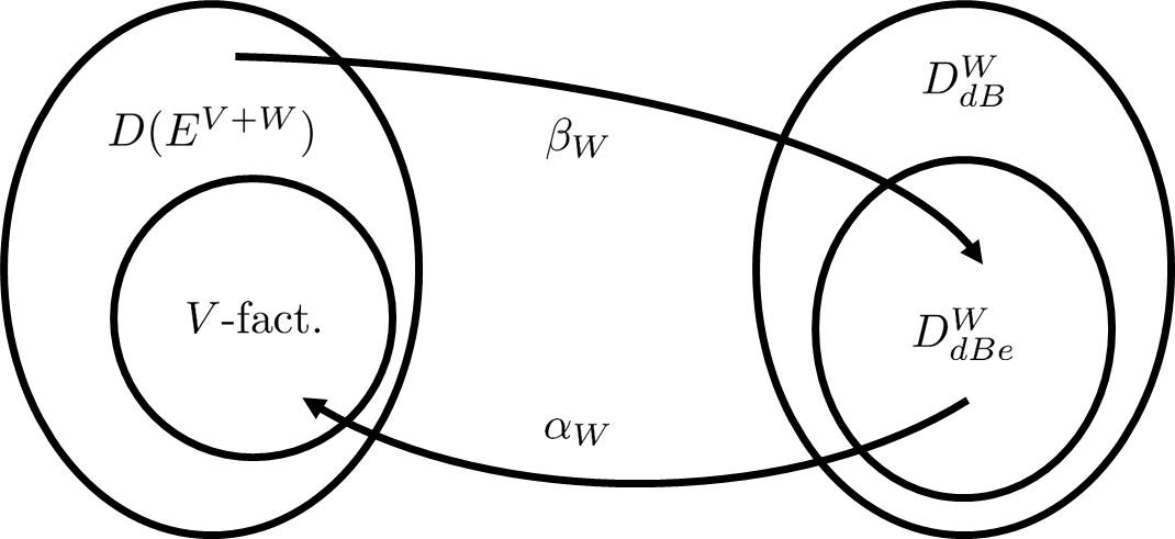
    DdBeW={gDdBW|×iWsupp g(i)XdBeW}.D^{W}_{dBe}=\{g\in D^{W}_{dB}\,|\,\times_{i\in W}\text{supp }g(i)\in X^{W}_{dBe}\}.
Refer to caption
(a)
Refer to caption
(b)
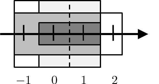
Figure 2: (a) The relation between global densities and de Bruijn densities. (b) An example of an approximation for W={1,0,1}𝑊101W=\{-1,0,1\}, V={0,1}𝑉01V=\{0,1\} and i=0𝑖0i=0. The thin and dark grey box that covers sites 00 and 111 is the factor at site 00. The medium box that covers sites 11-1 to 222 is the factor at site 111: the local state at site 222 depends on the local states from 11-1 to 111 (medium grey part). In the approximation (dashed line) the local state at 222 only depends on the one at 111. The thick box covering sites 11-1 to 111 is the factor at site 11-1. The local state at site 11-1 depends on the local states on sites 00 and 111 (light grey part). In the approximation the dependence stops again at the dashed line.

The idea behind extendable de Bruijn states is that every pattern can be extended to a global state by gluing suitable patterns on it. An example of an extendable de Bruijn density is βW(g)subscript𝛽𝑊𝑔\beta_{W}(g) in Example 3.1: for example pattern (10)10(10) at site 00 can be extended by (01)01(01) at site 111 to the global state (101)101(101), because the patterns coincide in the overlapping state 00. We find that this observation can be generalized.

Lemma 3.1.

im (βW)DdBeWim subscript𝛽𝑊subscriptsuperscript𝐷𝑊𝑑𝐵𝑒\text{im }(\beta_{W})\subseteq D^{W}_{dBe}.

Proof Let gim (βW)𝑔im subscript𝛽𝑊g\in\text{im }(\beta_{W}), jW𝑗𝑊j\in W and φEV𝜑superscript𝐸𝑉\varphi\in E^{V} with g(j)(φ)>0𝑔𝑗𝜑0g(j)(\varphi)>0. Then there is g~D(EV+W)~𝑔𝐷superscript𝐸𝑉𝑊\tilde{g}\in D(E^{V+W}) and ψEV+W𝜓superscript𝐸𝑉𝑊\psi\in E^{V+W} such that g~(ψ)>0~𝑔𝜓0\tilde{g}(\psi)>0 and σj(ψ)|V=φevaluated-atsubscript𝜎𝑗𝜓𝑉𝜑\sigma_{j}(\psi)|_{V}=\varphi. But furthermore already g(i)(σi(ψ)|V)>0𝑔𝑖evaluated-atsubscript𝜎𝑖𝜓𝑉0g(i)(\sigma_{i}(\psi)|_{V})>0 for all iW𝑖𝑊i\in W, and therefore ×iWsupp g(i)XdBeW\times_{i\in W}\text{supp }g(i)\in X^{W}_{dBe}. ∎

Because only the extendable de Bruijn densities are addressed by βWsubscript𝛽𝑊\beta_{W}, we only look for αWsubscript𝛼𝑊\alpha_{W} on them. Our choice is motivated by the following calculation, for which we first introduce some notation. For J𝐽J\subseteq\mathbb{Z} and A,BEJ𝐴𝐵superscript𝐸𝐽A,B\subseteq E^{J}, μ[A]=φAg(φ)𝜇delimited-[]𝐴subscript𝜑𝐴𝑔𝜑\mu[A]=\sum_{\varphi\in A}g(\varphi) denotes the distribution associated with gD(EJ)𝑔𝐷superscript𝐸𝐽g\in D(E^{J}), and μ[A|B]=μ[AB]μ[B]𝜇delimited-[]conditional𝐴𝐵𝜇delimited-[]𝐴𝐵𝜇delimited-[]𝐵\mu[A|B]=\frac{\mu[A\cap B]}{\mu[B]} the conditional probability. Furthermore

{ψ|J~J}={φEJ|φ|J~=ψ|J~}evaluated-at𝜓~𝐽𝐽conditional-set𝜑superscript𝐸𝐽evaluated-at𝜑~𝐽evaluated-at𝜓~𝐽\left\{\psi|^{J}_{\tilde{J}}\right\}=\left\{\varphi\in E^{J}\,|\,\varphi|_{\tilde{J}}=\psi|_{\tilde{J}}\right\}

for J~,J^,J~Jformulae-sequence~𝐽^𝐽~𝐽𝐽\tilde{J},\hat{J}\subseteq\mathbb{Z},\tilde{J}\subseteq J, J~J^,~𝐽^𝐽\tilde{J}\subseteq\hat{J}, and ψEJ^𝜓superscript𝐸^𝐽\psi\in E^{\hat{J}}, and we also write {ψ|J~}={ψ|J~J}evaluated-at𝜓~𝐽evaluated-at𝜓~𝐽𝐽\left\{\psi|_{\tilde{J}}\right\}=\left\{\psi|^{J}_{\tilde{J}}\right\} if J𝐽J is clear from the context. We calculate for iW𝑖𝑊i\in W and ψEV+W𝜓superscript𝐸𝑉𝑊\psi\in E^{V+W} that

μ[{ψ}]=𝜇delimited-[]𝜓absent\displaystyle\mu[\{\psi\}]= μ[{ψ|{t,,i}+V}]l=i+1uμ[{ψ|{t,,l}+V}]μ[{ψ|{t,,l}+V}]𝜇delimited-[]evaluated-at𝜓𝑡𝑖𝑉superscriptsubscriptproduct𝑙𝑖1𝑢𝜇delimited-[]evaluated-at𝜓𝑡𝑙𝑉𝜇delimited-[]evaluated-at𝜓𝑡𝑙subscript𝑉\displaystyle\mu[\{\psi|_{\{-t,...,i\}+V}\}]\,\prod_{l=i+1}^{u}\frac{\mu[\{\psi|_{\{-t,...,l\}+V}\}]}{\mu[\{\psi|_{\{-t,...,l\}+V_{-}}\}]}
=\displaystyle= k=ti1μ[{ψ|{kp}}|{ψ|{k,,i}+V+}]μ[{ψ|i+V}]l=i+1uμ[{ψ|{l+q}}|{ψ|{t,,l}+V}],\displaystyle\prod_{k=-t}^{i-1}\mu[\{\psi|_{\{k-p\}}\}\,|\,\{\psi|_{\{k,...,i\}+V_{+}}\}]\,\mu[\{\psi|_{i+V}\}]\,\prod_{l=i+1}^{u}\mu[\{\psi|_{\{l+q\}}\}\,|\,\{\psi|_{\{-t,...,l\}+V_{-}}\}],

where V+={p+1,,q}subscript𝑉𝑝1𝑞V_{+}=\{-p+1,...,q\} and V={p,,q1}subscript𝑉𝑝𝑞1V_{-}=\{-p,...,q-1\}. If there are no far-reaching correlations, we expect the following approximations to be suitable:

μ[{ψ|{kp}}|{ψ|{k,,i}+V+}]\displaystyle\mu[\{\psi|_{\{k-p\}}\}\,|\,\{\psi|_{\{k,...,i\}+V_{+}}\}] μ[{ψ|{kp}}|{ψ|k+V+}],\displaystyle\approx\mu[\{\psi|_{\{k-p\}}\}\,|\,\{\psi|_{k+V_{+}}\}],
μ[{ψ|{l+q}}|{ψ|{t,,l}+V}]\displaystyle\mu[\{\psi|_{\{l+q\}}\}\,|\,\{\psi|_{\{-t,...,l\}+V_{-}}\}] μ[{ψ|{l+q}}|{ψ|l+V}]\displaystyle\approx\mu[\{\psi|_{\{l+q\}}\}\,|\,\{\psi|_{l+V_{-}}\}]

for k{t,,i1}𝑘𝑡𝑖1k\in\{-t,...,i-1\} and l{i+1,,u}𝑙𝑖1𝑢l\in\{i+1,...,u\}. They resemble a Markov property of order |V|1𝑉1|V|-1 in space, see also Fig. 2b: a site’s state is independent from the states at sites that are more than |V|1𝑉1|V|-1 sites apart.

Lemma 3.2.

Let μjsubscript𝜇𝑗\mu_{j} be the distribution associated with βW(g)(j)D(EV)subscript𝛽𝑊𝑔𝑗𝐷superscript𝐸𝑉\beta_{W}(g)(j)\in D(E^{V}) for jW𝑗𝑊j\in W. Then

μ[{ψ|{kp}}|{ψ|k+V+}]\displaystyle\mu[\{\psi|_{\{k-p\}}\}\,|\,\{\psi|_{k+V_{+}}\}] =μk[{σk(ψ)|{p}}|{σk(ψ)|V+}],\displaystyle=\mu_{k}[\{\sigma_{k}(\psi)|_{\{-p\}}\}\,|\,\{\sigma_{k}(\psi)|_{V_{+}}\}],
μ[{ψ|i+V}]𝜇delimited-[]evaluated-at𝜓𝑖𝑉\displaystyle\mu[\{\psi|_{i+V}\}] =μi[{σi(ψ)|V}],absentsubscript𝜇𝑖delimited-[]evaluated-atsubscript𝜎𝑖𝜓𝑉\displaystyle=\mu_{i}[\{\sigma_{i}(\psi)|_{V}\}],
μ[{ψ|{lp}}|{ψ|l+V}]\displaystyle\mu[\{\psi|_{\{l-p\}}\}\,|\,\{\psi|_{l+V_{-}}\}] =μl[{σl(ψ)|{p}}|{σl(ψ)|V}],\displaystyle=\mu_{l}[\{\sigma_{l}(\psi)|_{\{-p\}}\}\,|\,\{\sigma_{l}(\psi)|_{V_{-}}\}],

for iW𝑖𝑊i\in W, k{t,,i1}𝑘𝑡𝑖1k\in\{-t,...,i-1\} and l{i+1,,u}𝑙𝑖1𝑢l\in\{i+1,...,u\}.

Proof Without loss of generality we prove the statement only for k{t,,i1}𝑘𝑡𝑖1k\in\{-t,...,i-1\}:

μ[{ψ|{kp}}|{ψ|k+V+}]\displaystyle\mu[\{\psi|_{\{k-p\}}\}\,|\,\{\psi|_{k+V_{+}}\}] =χ{ψ|k+V}g(χ)χ{ψ|k+V+}g(χ)=βW(g)(k)(σk(ψ)|V)φ{σk(ψ)|V+V}χ{σk(φ)|k+VV+W}g(χ)absentsubscript𝜒evaluated-at𝜓𝑘𝑉𝑔𝜒subscript𝜒evaluated-at𝜓𝑘subscript𝑉𝑔𝜒subscript𝛽𝑊𝑔𝑘evaluated-atsubscript𝜎𝑘𝜓𝑉subscript𝜑evaluated-atsubscript𝜎𝑘𝜓subscript𝑉𝑉subscript𝜒evaluated-atsubscript𝜎𝑘𝜑𝑘𝑉𝑉𝑊𝑔𝜒\displaystyle=\frac{\sum_{\chi\in\{\psi|_{k+V}\}}g(\chi)}{\sum_{\chi\in\{\psi|_{k+V_{+}}\}}g(\chi)}=\frac{\beta_{W}(g)(k)(\sigma_{k}(\psi)|_{V})}{\sum_{\varphi\in\left\{\sigma_{k}(\psi)|^{V}_{V_{+}}\right\}}\sum_{\chi\in\left\{\sigma_{-k}(\varphi)|_{k+V}^{V+W}\right\}}g(\chi)}
=βW(g)(k)(σk(ψ)|V)φ{σk(ψ)|V+V}βW(g)(k)(φ)=μk[{σk(ψ)|{p}}|{σk(ψ)|V+}].\displaystyle=\frac{\beta_{W}(g)(k)(\sigma_{k}(\psi)|_{V})}{\sum_{\varphi\in\left\{\sigma_{k}(\psi)|^{V}_{V_{+}}\right\}}\beta_{W}(g)(k)(\varphi)}=\mu_{k}[\{\sigma_{k}(\psi)|_{\{-p\}}\}\,|\,\{\sigma_{k}(\psi)|_{V_{+}}\}].\qquad\qed

Using the approximations introduced above and the lemma we find that

μ[{ψ}]𝜇delimited-[]𝜓absent\displaystyle\mu[\{\psi\}]\approx k=ti1μ[{ψ|{kp}}|{ψ|k+V+}]μ[{ψ|i+V}]l=i+1uμ[{ψ|{l+q}}|{ψ|l+V}]\displaystyle\prod_{k=-t}^{i-1}\mu[\{\psi|_{\{k-p\}}\}\,|\,\{\psi|_{k+V_{+}}\}]\,\mu[\{\psi|_{i+V}\}]\,\prod_{l=i+1}^{u}\mu[\{\psi|_{\{l+q\}}\}\,|\,\{\psi|_{l+V_{-}}\}]
=\displaystyle= k=ti1μk[{σk(ψ)|{p}}|{σk(ψ)|V+}]μi[{σi(ψ)|V}]l=i+1uμl[{σl(ψ)|{q}}|{σl(ψ)|V}].\displaystyle\prod_{k=-t}^{i-1}\mu_{k}[\{\sigma_{k}(\psi)|_{\{-p\}}\}\,|\,\{\sigma_{k}(\psi)|_{V_{+}}\}]\,\mu_{i}[\{\sigma_{i}(\psi)|_{V}\}]\,\prod_{l=i+1}^{u}\mu_{l}[\{\sigma_{l}(\psi)|_{\{q\}}\}\,|\,\{\sigma_{l}(\psi)|_{V_{-}}\}].

This way we are led to the following definition.

Definition 3.5.

Let iW𝑖𝑊i\in W. Then αW,i:DdBeWD(EV+W):subscript𝛼𝑊𝑖subscriptsuperscript𝐷𝑊𝑑𝐵𝑒𝐷superscript𝐸𝑉𝑊\alpha_{W,i}:D^{W}_{dBe}\to D(E^{V+W}) is given by

αW,i(g)(ψ)=k=ti1μk[{σk(ψ)|{p}}|{σk(ψ)|V+}]μi[{σi(ψ)|V}]l=i+1uμl[{σl(ψ)|{q}}|{σl(ψ)|V}],\alpha_{W,i}(g)(\psi)=\prod_{k=-t}^{i-1}\mu_{k}[\{\sigma_{k}(\psi)|_{\{-p\}}\}\,|\,\{\sigma_{k}(\psi)|_{V_{+}}\}]\,\mu_{i}[\{\sigma_{i}(\psi)|_{V}\}]\,\prod_{l=i+1}^{u}\mu_{l}[\{\sigma_{l}(\psi)|_{\{q\}}\}\,|\,\{\sigma_{l}(\psi)|_{V_{-}}\}],

where μjsubscript𝜇𝑗\mu_{j} is the distribution associated with g(j)D(EV)𝑔𝑗𝐷superscript𝐸𝑉g(j)\in D(E^{V}) for jW𝑗𝑊j\in W, and ψEV+W𝜓superscript𝐸𝑉𝑊\psi\in E^{V+W}.

For W={u},u,formulae-sequence𝑊𝑢𝑢W=\{u\},u\in\mathbb{Z}, the definition simplifies to α{u},u(g)(ψ)=g(u)(σu(ψ))subscript𝛼𝑢𝑢𝑔𝜓𝑔𝑢subscript𝜎𝑢𝜓\alpha_{\{u\},u}(g)(\psi)=g(u)(\sigma_{u}(\psi)). For V={0}𝑉0V=\{0\} the conditions vanish, and we get back simple multiplication, αW,i(g)(ψ)=kWg(k)(ψ(k))subscript𝛼𝑊𝑖𝑔𝜓subscriptproduct𝑘𝑊𝑔𝑘𝜓𝑘\alpha_{W,i}(g)(\psi)=\prod_{k\in W}g(k)(\psi(k)). We justify the general definition in the following lemma.

Lemma 3.3.

Let gDdBeW𝑔subscriptsuperscript𝐷𝑊𝑑𝐵𝑒g\in D^{W}_{dBe} and iW𝑖𝑊i\in W. Then αW,i(g)D(EV+W)subscript𝛼𝑊𝑖𝑔𝐷superscript𝐸𝑉𝑊\alpha_{W,i}(g)\in D(E^{V+W}).

Proof Let gDdBeW𝑔subscriptsuperscript𝐷𝑊𝑑𝐵𝑒g\in D^{W}_{dBe} and iW𝑖𝑊i\in W. αW,i(g)0not-equivalent-tosubscript𝛼𝑊𝑖𝑔0\alpha_{W,i}(g)\not\equiv 0 because there is at least one extendable pattern with nonzero probability. We prove that it is also normalized in the following. Without loss of generality we assume that i=u𝑖𝑢i=u. Then

φEV+WαW,u(g)(φ)=subscript𝜑superscript𝐸𝑉𝑊subscript𝛼𝑊𝑢𝑔𝜑absent\displaystyle\sum_{\varphi\in E^{V+W}}\alpha_{W,u}(g)(\varphi)= φEV+Wk=tu1μk[{σk(φ)|{p}}|{σk(φ)|V+}]μu[{σu(φ)|V}]\displaystyle\sum_{\varphi\in E^{V+W}}\prod_{k=-t}^{u-1}\mu_{k}[\{\sigma_{k}(\varphi)|_{\{-p\}}\}\,|\,\{\sigma_{k}(\varphi)|_{V_{+}}\}]\,\mu_{u}[\{\sigma_{u}(\varphi)|_{V}\}]\,
=\displaystyle= φ~EV+W\{t}φ{φ~|V+W\{t}V+W}μt[{σt(φ)|{p}}|{σt(φ~)|V+}]\displaystyle\sum_{\tilde{\varphi}\in E^{V+W\backslash\{-t\}}}\sum_{\varphi\in\left\{\tilde{\varphi}|_{V+W\backslash\{-t\}}^{V+W}\right\}}\mu_{-t}[\{\sigma_{-t}(\varphi)|_{\{-p\}}\}\,|\,\{\sigma_{-t}(\tilde{\varphi})|_{V_{+}}\}]
k=t+1u1μk[{σk(φ~)|{p}}|{σk(φ~)|V+}]μu[{σu(φ~)|V}]\displaystyle\prod_{k=-t+1}^{u-1}\mu_{k}[\{\sigma_{k}(\tilde{\varphi})|_{\{-p\}}\}\,|\,\{\sigma_{k}(\tilde{\varphi})|_{V_{+}}\}]\,\mu_{u}[\{\sigma_{u}(\tilde{\varphi})|_{V}\}]
=\displaystyle= φ~EV+W\{t}k=t+1u1μk[{σk(φ~)|{p}}|{σk(φ~)|V+}]μu[{σu(φ~)|V}]\displaystyle\sum_{\tilde{\varphi}\in E^{V+W\backslash\{-t\}}}\prod_{k=-t+1}^{u-1}\mu_{k}[\{\sigma_{k}(\tilde{\varphi})|_{\{-p\}}\}\,|\,\{\sigma_{k}(\tilde{\varphi})|_{V_{+}}\}]\,\mu_{u}[\{\sigma_{u}(\tilde{\varphi})|_{V}\}]
=\displaystyle= =φEu+Vμu[{σu(φ)|V}]=φEVg(φ)=1.subscript𝜑superscript𝐸𝑢𝑉subscript𝜇𝑢delimited-[]evaluated-atsubscript𝜎𝑢𝜑𝑉subscript𝜑superscript𝐸𝑉𝑔𝜑1\displaystyle...=\sum_{\varphi\in E^{u+V}}\mu_{u}[\{\sigma_{u}(\varphi)|_{V}\}]=\sum_{\varphi\in E^{V}}g(\varphi)=1.

The steps indicated by … follow by induction in |W|𝑊|W|. ∎

We find the following results for our construction.

Lemma 3.4.

Let iW𝑖𝑊i\in W and gim (βW)𝑔im subscript𝛽𝑊g\in\text{im }(\beta_{W}). Then αW,i(g)=αW,j(g)subscript𝛼𝑊𝑖𝑔subscript𝛼𝑊𝑗𝑔\alpha_{W,i}(g)=\alpha_{W,j}(g) for all i,jW𝑖𝑗𝑊i,j\in W.

Proof We show that αW,i(g)=αW,i+1(g)subscript𝛼𝑊𝑖𝑔subscript𝛼𝑊𝑖1𝑔\alpha_{W,i}(g)=\alpha_{W,i+1}(g) for all iW\{t}𝑖\𝑊𝑡i\in W\backslash\{-t\}. An index shift to the left can be proven analogously.

Note that μi[{σi(ψ)|V}]=g(i)(σi(ψ)|V)subscript𝜇𝑖delimited-[]evaluated-atsubscript𝜎𝑖𝜓𝑉𝑔𝑖evaluated-atsubscript𝜎𝑖𝜓𝑉\mu_{i}[\{\sigma_{i}(\psi)|_{V}\}]=g(i)(\sigma_{i}(\psi)|_{V}) and that for k{t,,i1}𝑘𝑡𝑖1k\in\{-t,...,i-1\} and l{i+1,,u}𝑙𝑖1𝑢l\in\{i+1,...,u\}

μk[{σk(ψ)|{p}}|{σk(ψ)|V+}]\displaystyle\mu_{k}[\{\sigma_{k}(\psi)|_{\{-p\}}\}\,|\,\{\sigma_{k}(\psi)|_{V_{+}}\}] =g(k)(σk(ψ)|V)χ{σk(ψ)|V+V}g(k)(χ),absent𝑔𝑘evaluated-atsubscript𝜎𝑘𝜓𝑉subscript𝜒evaluated-atsubscript𝜎𝑘𝜓subscript𝑉𝑉𝑔𝑘𝜒\displaystyle=\frac{g(k)(\sigma_{k}(\psi)|_{V})}{\sum_{\chi\in\left\{\sigma_{k}(\psi)|^{V}_{V_{+}}\right\}}g(k)(\chi)},
μl[{σl(ψ)|{q}}|{σl(ψ)|V}]\displaystyle\mu_{l}[\{\sigma_{l}(\psi)|_{\{q\}}\}\,|\,\{\sigma_{l}(\psi)|_{V_{-}}\}] =g(l)(σl(ψ)|V)χ{σl(ψ)|VV}g(l)(χ).absent𝑔𝑙evaluated-atsubscript𝜎𝑙𝜓𝑉subscript𝜒evaluated-atsubscript𝜎𝑙𝜓subscript𝑉𝑉𝑔𝑙𝜒\displaystyle=\frac{g(l)(\sigma_{l}(\psi)|_{V})}{\sum_{\chi\in\left\{\sigma_{l}(\psi)|^{V}_{V_{-}}\right\}}g(l)(\chi)}.

Therefore αW,i(g)(ψ)subscript𝛼𝑊𝑖𝑔𝜓\alpha_{W,i}(g)(\psi) and αW,i+1(g)(ψ)subscript𝛼𝑊𝑖1𝑔𝜓\alpha_{W,i+1}(g)(\psi) have the same numerator and only differ in the denominator. It is enough to show that a factor in the denominator may be shifted one step to the right: Let iW\{u}𝑖\𝑊𝑢i\in W\backslash\{u\} and g=βW(g~)𝑔subscript𝛽𝑊~𝑔g=\beta_{W}(\tilde{g}) for g~D(EV+W)~𝑔𝐷superscript𝐸𝑉𝑊\tilde{g}\in D(E^{V+W}). Then

χ{σi(ψ)|V+V}βW(g~)(i)(χ)subscript𝜒evaluated-atsubscript𝜎𝑖𝜓subscript𝑉𝑉subscript𝛽𝑊~𝑔𝑖𝜒\displaystyle\sum_{\chi\in\left\{\sigma_{i}(\psi)|^{V}_{V_{+}}\right\}}\beta_{W}(\tilde{g})(i)(\chi) =\displaystyle= χ{σi(ψ)|V+V}φ{σi(χ)|i+VV+W}g~(φ)subscript𝜒evaluated-atsubscript𝜎𝑖𝜓subscript𝑉𝑉subscript𝜑evaluated-atsubscript𝜎𝑖𝜒𝑖𝑉𝑉𝑊~𝑔𝜑\displaystyle\sum_{\chi\in\left\{\sigma_{i}(\psi)|^{V}_{V_{+}}\right\}}\,\,\sum_{\varphi\in\left\{\sigma_{-i}(\chi)|^{V+W}_{i+V}\right\}}\tilde{g}(\varphi)
=\displaystyle= φ{ψ|i+V+V+W}g~(φ)subscript𝜑evaluated-at𝜓𝑖subscript𝑉𝑉𝑊~𝑔𝜑\displaystyle\sum_{\varphi\in\left\{\psi|^{V+W}_{i+V_{+}}\right\}}\tilde{g}(\varphi) =\displaystyle= φ{ψ|i+1+VV+W}g~(φ)subscript𝜑evaluated-at𝜓𝑖1subscript𝑉𝑉𝑊~𝑔𝜑\displaystyle\sum_{\varphi\in\left\{\psi|^{V+W}_{i+1+V_{-}}\right\}}\tilde{g}(\varphi)
=\displaystyle= χ{σi+1(ψ)|VV}φ{σ(i+1)(χ)|i+1+VV+W}g~(φ)subscript𝜒evaluated-atsubscript𝜎𝑖1𝜓subscript𝑉𝑉subscript𝜑evaluated-atsubscript𝜎𝑖1𝜒𝑖1𝑉𝑉𝑊~𝑔𝜑\displaystyle\sum_{\chi\in\left\{\sigma_{i+1}(\psi)|^{V}_{V_{-}}\right\}}\,\,\sum_{\varphi\in\left\{\sigma_{-(i+1)}(\chi)|^{V+W}_{i+1+V}\right\}}\tilde{g}(\varphi) =\displaystyle= χ{σi+1(ψ)|VV}βW(g~)(i+1)(χ)subscript𝜒evaluated-atsubscript𝜎𝑖1𝜓subscript𝑉𝑉subscript𝛽𝑊~𝑔𝑖1𝜒\displaystyle\sum_{\chi\in\left\{\sigma_{i+1}(\psi)|^{V}_{V_{-}}\right\}}\beta_{W}(\tilde{g})(i+1)(\chi)\qquad\qed
Theorem 3.5.

Let gim(βW)𝑔imsubscript𝛽𝑊g\in\text{im}(\beta_{W}). Then βWαW,i(g)=gsubscript𝛽𝑊subscript𝛼𝑊𝑖𝑔𝑔\beta_{W}\alpha_{W,i}(g)=g for all iW𝑖𝑊i\in W.

Proof Let iW𝑖𝑊i\in W and gim(βW)𝑔imsubscript𝛽𝑊g\in\text{im}(\beta_{W}). We prove βWαW,i(g)(j)=g(j)subscript𝛽𝑊subscript𝛼𝑊𝑖𝑔𝑗𝑔𝑗\beta_{W}\alpha_{W,i}(g)(j)=g(j) without loss of generality only for j=u𝑗𝑢j=u.

With Lm. 3.4 and because a conditional distribution is a distribution as well, for ψEV𝜓superscript𝐸𝑉\psi\in E^{V}

βWαW,i(g)(u)(ψ)=subscript𝛽𝑊subscript𝛼𝑊𝑖𝑔𝑢𝜓absent\displaystyle\beta_{W}\alpha_{W,i}(g)(u)(\psi)= βWαW,u(g)(u)(ψ)=φ{σu(ψ)|u+VV+W}αW,u(g)(φ)subscript𝛽𝑊subscript𝛼𝑊𝑢𝑔𝑢𝜓subscript𝜑evaluated-atsubscript𝜎𝑢𝜓𝑢𝑉𝑉𝑊subscript𝛼𝑊𝑢𝑔𝜑\displaystyle\beta_{W}\alpha_{W,u}(g)(u)(\psi)=\sum_{\varphi\in\left\{\sigma_{-u}(\psi)|^{V+W}_{u+V}\right\}}\alpha_{W,u}(g)(\varphi)
=\displaystyle= φ~{σu(ψ)|u+VV+W\{t}}φ{φ~|V+W\{t}V+W}μt[{σt(φ)|{p}}|{σt(φ~)|V+}]\displaystyle\sum_{\tilde{\varphi}\in\left\{\sigma_{-u}(\psi)|^{V+W\backslash\{-t\}}_{u+V}\right\}}\,\,\sum_{\varphi\in\left\{\tilde{\varphi}|^{V+W}_{V+W\backslash\{-t\}}\right\}}\mu_{-t}[\{\sigma_{-t}(\varphi)|_{\{-p\}}\}\,|\,\{\sigma_{-t}(\tilde{\varphi})|_{V_{+}}\}]
k=t+1u1μk[{σk(φ~)|{p}}|{σk(φ~)|V+}]μu[{σu(φ~)|V}]\displaystyle\prod_{k=-t+1}^{u-1}\mu_{k}[\{\sigma_{k}(\tilde{\varphi})|_{\{-p\}}\}\,|\,\{\sigma_{k}(\tilde{\varphi})|_{V_{+}}\}]\,\mu_{u}[\{\sigma_{u}(\tilde{\varphi})|_{V}\}]\,
=\displaystyle= φ~{σu(ψ)|u+VV+W\{t}}k=t+1u1μk[{σk(φ~)|{p}}|{σk(φ~)|V+}]μu[{σu(φ~)|V}]\displaystyle\sum_{\tilde{\varphi}\in\left\{\sigma_{-u}(\psi)|^{V+W\backslash\{-t\}}_{u+V}\right\}}\,\,\prod_{k=-t+1}^{u-1}\mu_{k}[\{\sigma_{k}(\tilde{\varphi})|_{\{-p\}}\}\,|\,\{\sigma_{k}(\tilde{\varphi})|_{V_{+}}\}]\,\mu_{u}[\{\sigma_{u}(\tilde{\varphi})|_{V}\}]\,
=\displaystyle= =g(u)(ψ).𝑔𝑢𝜓\displaystyle...=g(u)(\psi).

The last steps follow by induction in |W|𝑊|W|. ∎

Now we focus on global densities that are preserved under αW,iβWsubscript𝛼𝑊𝑖subscript𝛽𝑊\alpha_{W,i}\beta_{W} for all iW𝑖𝑊i\in W. We will see that they enable an algebraic interpretation of βWsubscript𝛽𝑊\beta_{W}. Our choice of αW,isubscript𝛼𝑊𝑖\alpha_{W,i} is further justified thereby.

Definition 3.6.

gD(EV+W)𝑔𝐷superscript𝐸𝑉𝑊g\in D(E^{V+W}) is called V𝑉V-factorizable, if g=αW,iβW(g)𝑔subscript𝛼𝑊𝑖subscript𝛽𝑊𝑔g=\alpha_{W,i}\beta_{W}(g) for all iW𝑖𝑊i\in W.

An example of a {0,1}01\{0,1\}-factorizable density is g~~𝑔\tilde{g} in Ex. 3.1. g𝑔g in the same example however has correlations over 222 sites and is not {0,1}01\{0,1\}-factorizable: a state only has positive probability if the local states at sites 00 and 222 differ. The correlations are ignored by βWsubscript𝛽𝑊\beta_{W}.

Lemma 3.6.

Let iW𝑖𝑊i\in W and gim (βW)𝑔im subscript𝛽𝑊g\in\text{im }(\beta_{W}). Then αW,i(g)subscript𝛼𝑊𝑖𝑔\alpha_{W,i}(g) is V-factorizable.

Proof Let gim (βW)𝑔im subscript𝛽𝑊g\in\text{im }(\beta_{W}) and i,jW𝑖𝑗𝑊i,j\in W. Then by Lm. 3.4 and Thm. 3.5

αW,i(g)=αW,j(g)=αW,jβWαW,i(g),subscript𝛼𝑊𝑖𝑔subscript𝛼𝑊𝑗𝑔subscript𝛼𝑊𝑗subscript𝛽𝑊subscript𝛼𝑊𝑖𝑔\displaystyle\alpha_{W,i}(g)=\alpha_{W,j}(g)=\alpha_{W,j}\beta_{W}\alpha_{W,i}(g),

and hence αW,i(g)subscript𝛼𝑊𝑖𝑔\alpha_{W,i}(g) is V-factorizable. ∎

Theorem 3.7.

For all gD(EV+W)𝑔𝐷superscript𝐸𝑉𝑊g\in D(E^{V+W}) there is a V𝑉V-factorizable g~D(EV+W)~𝑔𝐷superscript𝐸𝑉𝑊\tilde{g}\in D(E^{V+W}) such that βW(g~)=βW(g)subscript𝛽𝑊~𝑔subscript𝛽𝑊𝑔\beta_{W}(\tilde{g})=\beta_{W}(g).

Proof Let gD(EV+W)𝑔𝐷superscript𝐸𝑉𝑊g\in D(E^{V+W}) and choose g~=αW,uβW(g)~𝑔subscript𝛼𝑊𝑢subscript𝛽𝑊𝑔\tilde{g}=\alpha_{W,u}\beta_{W}(g). Then g~~𝑔\tilde{g} is V𝑉V-factorizable by Lm. 3.6, and the definition does not depend on the site u𝑢u. Furthermore βW(g~)=βWαW,uβW(g)=βW(g)subscript𝛽𝑊~𝑔subscript𝛽𝑊subscript𝛼𝑊𝑢subscript𝛽𝑊𝑔subscript𝛽𝑊𝑔\beta_{W}(\tilde{g})=\beta_{W}\alpha_{W,u}\beta_{W}(g)=\beta_{W}(g) by Thm. 3.5. ∎

βWsubscript𝛽𝑊\beta_{W} induces equivalence classes on D(EV+W)𝐷superscript𝐸𝑉𝑊D(E^{V+W}) by collecting all global densities with the same image in one class. According to Thm. 3.7 each equivalence class contains at least one V𝑉V-factorizable state. Moreover, we know that there is exactly one such state, because βWsubscript𝛽𝑊\beta_{W} is injective on these states by definition. It is given as the image under αW,iβWsubscript𝛼𝑊𝑖subscript𝛽𝑊\alpha_{W,i}\beta_{W} of any state in the class for any iW𝑖𝑊i\in W. Therefore it is possible to choose the V𝑉V-factorizable states as the representatives of the equivalence classes. These representatives are preserved under αW,iβWsubscript𝛼𝑊𝑖subscript𝛽𝑊\alpha_{W,i}\beta_{W} for any iW𝑖𝑊i\in W. Ex. 3.1 provides an example: g𝑔g and g~~𝑔\tilde{g} are in the same equivalence class, and g~=αW,0βW(g)~𝑔subscript𝛼𝑊0subscript𝛽𝑊𝑔\tilde{g}=\alpha_{W,0}\beta_{W}(g) is the unique V𝑉V-factorizable representative of the class.

However, in general αW,i(g)subscript𝛼𝑊𝑖𝑔\alpha_{W,i}(g) is not V𝑉V-factorizable if gDdBeW\im (βW)𝑔\subscriptsuperscript𝐷𝑊𝑑𝐵𝑒im subscript𝛽𝑊g\in D^{W}_{dBe}\backslash\text{im }(\beta_{W}). There is a degree of freedom in how to map a density collection to a global density on this set. We choose the arithmetic mean over all αW,isubscript𝛼𝑊𝑖\alpha_{W,i}, where iW𝑖𝑊i\in W. Note that for gim (βW)𝑔im subscript𝛽𝑊g\in\text{im }(\beta_{W}) the definition then coincides with any αW,isubscript𝛼𝑊𝑖\alpha_{W,i}.

Definition 3.7.

αW:DdBeWD(EV+W):subscript𝛼𝑊superscriptsubscript𝐷𝑑𝐵𝑒𝑊𝐷superscript𝐸𝑉𝑊\alpha_{W}:D_{dBe}^{W}\to D(E^{V+W}) is given by αW(g)=1|W|iWαW,i(g)subscript𝛼𝑊𝑔1𝑊subscript𝑖𝑊subscript𝛼𝑊𝑖𝑔\alpha_{W}(g)=\frac{1}{|W|}\sum_{i\in W}\alpha_{W,i}(g).

It is clear that αW(g)subscript𝛼𝑊𝑔\alpha_{W}(g) is a density by similar reasoning as for αW,i(g)subscript𝛼𝑊𝑖𝑔\alpha_{W,i}(g).

3.3 General Cellular Probabilistic Automata

With the de Bruijn calculus at hand we can now generalize the definition of CPA to general V𝑉V.

Definition 3.8.

As before let I={1,,m}𝐼1𝑚I=\{1,...,m\}, U={r,,s}𝑈𝑟𝑠U=\{-r,...,s\}, V={p,,q}𝑉𝑝𝑞V=\{-p,...,q\} for p,q,r,s,m0𝑝𝑞𝑟𝑠𝑚subscript0p,q,r,s,m\in\mathbb{N}_{0} with m1,1+p+q+r+smformulae-sequence𝑚11𝑝𝑞𝑟𝑠𝑚m\geq 1,1+p+q+r+s\leq m and K={1,,r}{ms+1,,m}𝐾1𝑟𝑚𝑠1𝑚K=\{1,...,r\}\cup\{m-s+1,...,m\}. We now set il=1+p+rsubscript𝑖𝑙1𝑝𝑟i_{l}=1+p+r, ir=mqssubscript𝑖𝑟𝑚𝑞𝑠i_{r}=m-q-s and I~={il,,ir}~𝐼subscript𝑖𝑙subscript𝑖𝑟\tilde{I}=\{i_{l},...,i_{r}\}.

  • i)

    We set α^:DdBeI~DBC(EI),gα^(g):^𝛼formulae-sequencesuperscriptsubscript𝐷𝑑𝐵𝑒~𝐼subscript𝐷𝐵𝐶superscript𝐸𝐼maps-to𝑔^𝛼𝑔\hat{\alpha}:D_{dBe}^{\tilde{I}}\to D_{BC}(E^{I}),\,g\mapsto\hat{\alpha}(g) with

    α^(g)(ψ)^𝛼𝑔𝜓\displaystyle\hat{\alpha}(g)(\psi) ={αI~(g)(ψ|{1+r,,ms}) if ψ|K=ρ0 else absentcasessubscript𝛼~𝐼𝑔evaluated-at𝜓1𝑟𝑚𝑠evaluated-at if 𝜓𝐾𝜌0 else \displaystyle=\left\{\begin{array}[]{ll}\alpha_{\tilde{I}}(g)(\psi|_{\{1+r,...,m-s\}})&\mbox{ if }\psi|_{K}=\rho\\ 0&\mbox{ else }\\ \end{array}\right.
  • ii)

    and β^:DBC(EI)DdBeI~,gβ^(g):^𝛽formulae-sequencesubscript𝐷𝐵𝐶superscript𝐸𝐼superscriptsubscript𝐷𝑑𝐵𝑒~𝐼maps-to𝑔^𝛽𝑔\hat{\beta}:D_{BC}(E^{I})\to D_{dBe}^{\tilde{I}},\,g\mapsto\hat{\beta}(g) with

    β^(g)(i)(ψ)=χ|i+V=σi(ψ)χEI s. t. g(χ).^𝛽𝑔𝑖𝜓subscript𝜒superscript𝐸𝐼 s. t. evaluated-at𝜒𝑖𝑉subscript𝜎𝑖𝜓𝑔𝜒\hat{\beta}(g)(i)(\psi)=\sum_{\overset{\chi\in E^{I}\text{ s. t. }}{\chi|_{i+V}=\sigma_{-i}(\psi)}}g(\chi).
Definition 3.9.

A cellular probabilistic automaton (CPA) is a tuple (I,U,V,E,f0)𝐼𝑈𝑉𝐸subscript𝑓0(I,U,V,E,f_{0}), where for m,p,q,r,s0𝑚𝑝𝑞𝑟𝑠subscript0m,p,q,r,s\in\mathbb{N}_{0} with m1𝑚1m\geq 1 and 1+p+q+r+sm1𝑝𝑞𝑟𝑠𝑚1+p+q+r+s\leq m

  • i)

    I={1,,m}𝐼1𝑚I=\{1,...,m\} is a finite grid,

  • ii)

    U={r,,s}𝑈𝑟𝑠U=\{-r,...,s\} is the neighborhood,

  • iii)

    V={p,,q}𝑉𝑝𝑞V=\{-p,...,q\} gives rise to de Bruijn patterns,

  • iv)

    E𝐸E is a finite set of local states

  • v)

    and f0:EU+VD(EV):subscript𝑓0superscript𝐸𝑈𝑉𝐷superscript𝐸𝑉f_{0}:E^{U+V}\rightarrow D(E^{V}) is the local function.

With the boundary conditions ρEK𝜌superscript𝐸𝐾\rho\in E^{K} for K={1,,r}{ms+1,,m}𝐾1𝑟𝑚𝑠1𝑚K=\{1,...,r\}\cup\{m-s+1,...,m\} and the definitions il=1+p+rsubscript𝑖𝑙1𝑝𝑟i_{l}=1+p+r, ir=mqssubscript𝑖𝑟𝑚𝑞𝑠i_{r}=m-q-s, I~={il,,ir}~𝐼subscript𝑖𝑙subscript𝑖𝑟\tilde{I}=\{i_{l},...,i_{r}\}, U~(i)={u¯(i),,u¯(i)}~𝑈𝑖¯𝑢𝑖¯𝑢𝑖\tilde{U}(i)=\{-\underline{u}(i),...,\overline{u}(i)\} and u¯,u¯:I~U:¯𝑢¯𝑢~𝐼𝑈\underline{u},\overline{u}:\tilde{I}\to U with

u¯(i)¯𝑢𝑖\displaystyle\underline{u}(i) ={iil if i{il,,il+r1}r else ,absentcases𝑖subscript𝑖𝑙 if 𝑖subscript𝑖𝑙subscript𝑖𝑙𝑟1𝑟 else \displaystyle=\left\{\begin{array}[]{ll}i-i_{l}&\mbox{ if }i\in\{i_{l},...,i_{l}+r-1\}\\ r&\mbox{ else }\\ \end{array}\right.,
u¯(i)¯𝑢𝑖\displaystyle\overline{u}(i) ={iri if i{irs+1,,ir}s else ,absentcasessubscript𝑖𝑟𝑖 if 𝑖subscript𝑖𝑟𝑠1subscript𝑖𝑟𝑠 else \displaystyle=\left\{\begin{array}[]{ll}i_{r}-i&\mbox{ if }i\in\{i_{r}-s+1,...,i_{r}\}\\ s&\mbox{ else }\\ \end{array}\right.,

the global function is given by

f:DdBeI~DdBeI~,gf(g),:𝑓formulae-sequencesuperscriptsubscript𝐷𝑑𝐵𝑒~𝐼superscriptsubscript𝐷𝑑𝐵𝑒~𝐼maps-to𝑔𝑓𝑔f:D_{dBe}^{\tilde{I}}\rightarrow D_{dBe}^{\tilde{I}},\quad g\mapsto f(g),
f(g)(i)(ψ)=for kKi+U+VφEU+V s.t. φ(ki)=ρ(k)αU~(i)(σi(g)|U~(i))(φ|V+U~(i))f0(φ)(ψ).𝑓𝑔𝑖𝜓subscript𝜑superscript𝐸𝑈𝑉 s.t. 𝜑𝑘𝑖𝜌𝑘for 𝑘𝐾𝑖𝑈𝑉subscript𝛼~𝑈𝑖evaluated-atsubscript𝜎𝑖𝑔~𝑈𝑖evaluated-at𝜑𝑉~𝑈𝑖subscript𝑓0𝜑𝜓f(g)(i)(\psi)=\sum_{\overset{\varphi\in E^{U+V}\text{ s.t. }\varphi(k-i)=\rho(k)}{\text{for }k\in K\cap i+U+V}}\alpha_{\tilde{U}(i)}(\sigma_{i}(g)|_{\tilde{U}(i)})(\varphi|_{V+\tilde{U}(i)})\cdot f_{0}(\varphi)(\psi).

The trajectory starting with g0(D(EV))I~superscript𝑔0superscript𝐷superscript𝐸𝑉~𝐼g^{0}\in(D(E^{V}))^{\tilde{I}} is given by the sequence (gn)nsubscriptsuperscript𝑔𝑛𝑛(g^{n})_{n\in\mathbb{N}}, where gn=f(gn1)superscript𝑔𝑛𝑓superscript𝑔𝑛1g^{n}=f(g^{n-1}) for n+𝑛superscriptn\in\mathbb{N}^{+}.

See Fig. 3 for a sketch of how the CPA works on general patterns. Remark that f0subscript𝑓0f_{0} is not arbitrary but connected to a dynamical system with the locality property. By investigating this relation we can assure that the global function is well-defined.
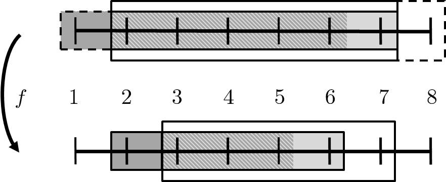
Refer to caption
Figure 3: An example of a CPA with I={1,,8}𝐼18I=\{1,...,8\}, U={1,0,1}𝑈101U=\{-1,0,1\} and V={2,,2}𝑉22V=\{-2,...,2\}. The global function considers patterns located at I~={4,5}~𝐼45\tilde{I}=\{4,5\} and sketched in the image (lower part) by rectangles of small and large height, respectively. The corresponding preimage patterns (upper part) are larger due to the neighborhood, and their probability of occurence is influenced by boundary conditions (dashed parts). From an implementational point of view, V𝑉V may be constructed from V~={2,,1}~𝑉21\tilde{V}=\{-2,...,1\} and W={0,1}𝑊01W=\{0,1\}, see Section 5.2: Focus on a pattern at site 444. The transition probability from a preimage pattern is calculated from the information about two subtransitions between light and dark grey subpatterns.
Lemma 3.8.

f(DdBeI~)DdBeI~𝑓superscriptsubscript𝐷𝑑𝐵𝑒~𝐼superscriptsubscript𝐷𝑑𝐵𝑒~𝐼f(D_{dBe}^{\tilde{I}})\subseteq D_{dBe}^{\tilde{I}}.

Proof Because DdBeI~=(D(EV))I~superscriptsubscript𝐷𝑑𝐵𝑒~𝐼superscript𝐷superscript𝐸𝑉~𝐼D_{dBe}^{\tilde{I}}=(D(E^{V}))^{\tilde{I}} for |V|=1𝑉1|V|=1, the statement is trivial in this case. So we focus on |V|>1𝑉1|V|>1. We show that without loss of generality any pattern in the support of any site in the image can be extended to the right by a pattern in the support of the neighboring site.

Let gDdBeI~,i{il,,ir1}formulae-sequence𝑔superscriptsubscript𝐷𝑑𝐵𝑒~𝐼𝑖subscript𝑖𝑙subscript𝑖𝑟1g\in D_{dBe}^{\tilde{I}},i\in\{i_{l},...,i_{r}-1\} and ψsupp f(g)(i)𝜓supp 𝑓𝑔𝑖\psi\in\text{supp }f(g)(i). By the construction of f𝑓f and αU~(i)subscript𝛼~𝑈𝑖\alpha_{\tilde{U}(i)} we know that there is φEU+V𝜑superscript𝐸𝑈𝑉\varphi\in E^{U+V} such that σj(φ)|Vsupp(g)(i+j)evaluated-atsubscript𝜎𝑗𝜑𝑉supp𝑔𝑖𝑗\sigma_{j}(\varphi)|_{V}\in\text{supp}(g)(i+j) for all jU𝑗𝑈j\in U and f0(φ)(ψ)>0subscript𝑓0𝜑𝜓0f_{0}(\varphi)(\psi)>0. Because of the extension property of the preimage g𝑔g we can find φ~EU+V~𝜑superscript𝐸𝑈𝑉\tilde{\varphi}\in E^{U+V} such that σj(φ~)|V=σj+1(φ)|Vsupp (g)(i+1+j)evaluated-atsubscript𝜎𝑗~𝜑𝑉evaluated-atsubscript𝜎𝑗1𝜑𝑉supp 𝑔𝑖1𝑗\sigma_{j}(\tilde{\varphi})|_{V}=\sigma_{j+1}(\varphi)|_{V}\in\text{supp }(g)(i+1+j) for all j{r,,s1}𝑗𝑟𝑠1j\in\{-r,...,s-1\} and σs(φ~)|Vsupp (g)(i+1+s)evaluated-atsubscript𝜎𝑠~𝜑𝑉supp 𝑔𝑖1𝑠\sigma_{s}(\tilde{\varphi})|_{V}\in\text{supp }(g)(i+1+s).

This enables us to find ψ~supp f(g)(i+1)~𝜓supp 𝑓𝑔𝑖1\tilde{\psi}\in\text{supp }f(g)(i+1) such that ψ~|V=σ1(ψ|V+)evaluated-at~𝜓subscript𝑉subscript𝜎1evaluated-at𝜓subscript𝑉\tilde{\psi}|_{V_{-}}=\sigma_{1}(\psi|_{V_{+}}), as we will show in the following. Hence the pattern ψ𝜓\psi may be extended to the right by ψ~~𝜓\tilde{\psi}, and the proof is complete.

Since f0(φ)(ψ)>0subscript𝑓0𝜑𝜓0f_{0}(\varphi)(\psi)>0 and the partition is uniform, there is an ϵitalic-ϵ\epsilon-ball Bϵsubscript𝐵italic-ϵB_{\epsilon} with respect to the 2-norm in mnsuperscript𝑚𝑛\mathbb{R}^{mn}, ϵ>0,italic-ϵ0\epsilon>0, such that

BϵΩσi(φ)Φτ(Ωσi(ψ)).subscript𝐵italic-ϵsubscriptΩsubscript𝜎𝑖𝜑superscriptΦ𝜏subscriptΩsubscript𝜎𝑖𝜓B_{\epsilon}\subseteq\Omega_{\sigma_{-i}(\varphi)}\cap\Phi^{-\tau}(\Omega_{\sigma_{-i}(\psi)}).

Because the set is just restricted on sites i+U+V𝑖𝑈𝑉i+U+V due to the locality property, we may independently restrict at site i+1+q+s𝑖1𝑞𝑠i+1+q+s and can still find ϵ>0superscriptitalic-ϵ0\epsilon^{\prime}>0 with

Bϵsubscript𝐵superscriptitalic-ϵ\displaystyle B_{\epsilon^{\prime}} Ωσi(φ)Ωσ(i+1)(φ~(q+s))Φτ(Ωσi(ψ))absentsubscriptΩsubscript𝜎𝑖𝜑subscriptΩsubscript𝜎𝑖1~𝜑𝑞𝑠superscriptΦ𝜏subscriptΩsubscript𝜎𝑖𝜓\displaystyle\subseteq\Omega_{\sigma_{-i}(\varphi)}\cap\Omega_{\sigma_{-(i+1)}(\tilde{\varphi}(q+s))}\cap\Phi^{-\tau}(\Omega_{\sigma_{-i}(\psi)})
Ωσi(φ|V++U)Ωσ(i+1)(φ~|q+s)Φτ(Ωσi(ψ|V+))absentsubscriptΩsubscript𝜎𝑖evaluated-at𝜑subscript𝑉𝑈subscriptΩsubscript𝜎𝑖1evaluated-at~𝜑𝑞𝑠superscriptΦ𝜏subscriptΩsubscript𝜎𝑖evaluated-at𝜓subscript𝑉\displaystyle\subseteq\Omega_{\sigma_{-i}(\varphi|_{V_{+}+U})}\cap\Omega_{\sigma_{-(i+1)}(\tilde{\varphi}|_{q+s})}\cap\Phi^{-\tau}(\Omega_{\sigma_{-i}(\psi|_{V_{+}})})
=Ωσ(i+1)(φ~)Φτ(Ωσi(ψ|V+)).absentsubscriptΩsubscript𝜎𝑖1~𝜑superscriptΦ𝜏subscriptΩsubscript𝜎𝑖evaluated-at𝜓subscript𝑉\displaystyle=\Omega_{\sigma_{-(i+1)}(\tilde{\varphi})}\cap\Phi^{-\tau}(\Omega_{\sigma_{-i}(\psi|_{V_{+}})}).

In the second line we have again used the locality property, and the equality sign holds due to σi(φ|V++U)=σ(i+1)(φ~|V+U)subscript𝜎𝑖evaluated-at𝜑subscript𝑉𝑈subscript𝜎𝑖1evaluated-at~𝜑subscript𝑉𝑈\sigma_{-i}(\varphi|_{V_{+}+U})=\sigma_{-(i+1)}(\tilde{\varphi}|_{V_{-}+U}). We now define ψ~EV~𝜓superscript𝐸𝑉\tilde{\psi}\in E^{V} by ψ~|V=σ1(ψ|V+)evaluated-at~𝜓subscript𝑉subscript𝜎1evaluated-at𝜓subscript𝑉\tilde{\psi}|_{V_{-}}=\sigma_{1}(\psi|_{V_{+}}) and choose ψ~(q)~𝜓𝑞\tilde{\psi}(q) such that there is ϵ′′>0superscriptitalic-ϵ′′0\epsilon^{\prime\prime}>0 with

Bϵ′′BϵΦτ(Ωσ(i+1)(ψ(q))).subscript𝐵superscriptitalic-ϵ′′subscript𝐵superscriptitalic-ϵsuperscriptΦ𝜏subscriptΩsubscript𝜎𝑖1𝜓𝑞B_{\epsilon^{\prime\prime}}\subseteq B_{\epsilon^{\prime}}\cap\Phi^{-\tau}(\Omega_{\sigma_{-(i+1)}(\psi(q))}).

Therefore

Bϵ′′Ωσ(i+1)(φ~)Φτ(Ωσ(i+1)(ψ~)),subscript𝐵superscriptitalic-ϵ′′subscriptΩsubscript𝜎𝑖1~𝜑superscriptΦ𝜏subscriptΩsubscript𝜎𝑖1~𝜓B_{\epsilon^{\prime\prime}}\subseteq\Omega_{\sigma_{-(i+1)}(\tilde{\varphi})}\cap\Phi^{-\tau}(\Omega_{\sigma_{-(i+1)}(\tilde{\psi})}),

f0(φ~)(ψ~)>0subscript𝑓0~𝜑~𝜓0f_{0}(\tilde{\varphi})(\tilde{\psi})>0, and ψ~supp f(g)(i+1)~𝜓supp 𝑓𝑔𝑖1\tilde{\psi}\in\text{supp }f(g)(i+1). ∎

We denote the case of il=irsubscript𝑖𝑙subscript𝑖𝑟i_{l}=i_{r} with Vmaxsubscript𝑉V_{\max} and find that α^β^(g)=g^𝛼^𝛽𝑔𝑔\hat{\alpha}\hat{\beta}(g)=g for all gDBC(EI)𝑔subscript𝐷𝐵𝐶superscript𝐸𝐼g\in{D_{BC}(E^{I})} and β^α^(g)=g^𝛽^𝛼𝑔𝑔\hat{\beta}\hat{\alpha}(g)=g for all g(D(EV))I~𝑔superscript𝐷superscript𝐸𝑉~𝐼g\in(D(E^{V}))^{\tilde{I}}. Furthermore U~(I~)={0}~𝑈~𝐼0\tilde{U}(\tilde{I})=\{0\} in this case, and it can be calculated for gDdBeI~𝑔superscriptsubscript𝐷𝑑𝐵𝑒~𝐼g\in D_{dBe}^{\tilde{I}} and φEU+V𝜑superscript𝐸𝑈𝑉\varphi\in E^{U+V} that

α{0}(σil(g))(φ|V)=g(il)(φ|V).subscript𝛼0subscript𝜎subscript𝑖𝑙𝑔evaluated-at𝜑𝑉𝑔subscript𝑖𝑙evaluated-at𝜑𝑉\alpha_{\{0\}}(\sigma_{i_{l}}(g))(\varphi|_{V})=g(i_{l})(\varphi|_{V}).

For ψEV𝜓superscript𝐸𝑉\psi\in E^{V} then

f(g)(il)(ψ)=g(il)(φ|V)f0(φ)(ψ),𝑓𝑔subscript𝑖𝑙𝜓𝑔subscript𝑖𝑙evaluated-at𝜑𝑉subscript𝑓0𝜑𝜓f(g)(i_{l})(\psi)=\sum g(i_{l})(\varphi|_{V})\cdot f_{0}(\varphi)(\psi),

where the sum is taken over all φEU+V𝜑superscript𝐸𝑈𝑉\varphi\in E^{U+V} such that the boundary conditions are fulfilled. For Vmaxsubscript𝑉V_{\max} the evolution of the global density is calculated directly, and locality is completely omitted.

4 Consistency

The goal is to prove in Section 4.3 that time evolution of probability densities under CPA can approximate time evolution under FPO arbitrarily close. We prepare this consistency result by investigating first the two features state space discretization and locality in more depth in Sections 4.1 and 4.2, respectively.

4.1 State Space Discretization

In this section we just compare the discretized FPO to the real FPO without considering locality. There are many ways to study distances between probability measures [9]. In our density based formulation we use the 1superscript1\mathcal{L}^{1}-norm for probability densities which leads to the notion of strong convergence in the literature [30]. It is well-known that in this norm the discretized operator converges pointwise to the FPO for increasing state space resolution in the case of Lipschitz continuous input densities [26]. But because the image under RPΦτ𝑅subscript𝑃superscriptΦ𝜏RP_{\Phi^{\tau}} is in general not continuous, for iteration we need to generalize the result to 1superscript1\mathcal{L}^{1}-functions. We start with some necessary tools.

A subset MX𝑀𝑋M\subseteq X of a metric space (X,d)𝑋𝑑(X,d) is called totally bounded, if for every ϵ>0italic-ϵ0\epsilon>0 there exist n𝑛n\in\mathbb{N} and x1,,xnMsubscript𝑥1subscript𝑥𝑛𝑀x_{1},...,x_{n}\in M such that

Mi=1n{xX|d(x,xi)<ϵ}.𝑀superscriptsubscript𝑖1𝑛conditional-set𝑥𝑋𝑑𝑥subscript𝑥𝑖italic-ϵM\subseteq\bigcup_{i=1}^{n}\{x\in X\,|\,d(x,x_{i})<\epsilon\}.

Totally bounded subsets of p(n)superscript𝑝superscript𝑛\mathcal{L}^{p}(\mathbb{R}^{n}) can be alternatively characterized in a functional analytical sense by the theorem of Kolmogorov-Riesz [15, 45]. In the following |.||.| denotes the 2-norm in nsuperscript𝑛\mathbb{R}^{n}.

Theorem 4.1.

Kolmogorov-Riesz

A set Mp(n)𝑀superscript𝑝superscript𝑛M\subset\mathcal{L}^{p}(\mathbb{R}^{n}), 1p<1𝑝1\leq p<\infty is totally bounded if and only if the following criteria are fulfilled:

  • i)

    M𝑀M is bounded in p(n)superscript𝑝superscript𝑛\mathcal{L}^{p}(\mathbb{R}^{n}), i.e. supgMgp<subscriptsupremum𝑔𝑀subscriptnorm𝑔𝑝\sup_{g\in M}\|g\|_{p}<\infty.

  • ii)

    For every ϵ>0italic-ϵ0\epsilon>0 there is some R𝑅R so that for every gM𝑔𝑀g\in M

    |v|>R|g(v)|p𝑑v<ϵp.subscript𝑣𝑅superscript𝑔𝑣𝑝differential-d𝑣superscriptitalic-ϵ𝑝\int_{|v|>R}|g(v)|^{p}dv<\epsilon^{p}.
  • iii)

    For every ϵ>0italic-ϵ0\epsilon>0 there is δ>0𝛿0\delta>0 so that for every gM𝑔𝑀g\in M and wn𝑤superscript𝑛w\in\mathbb{R}^{n} with |w|<δ𝑤𝛿|w|<\delta

    n|g(v+w)g(v)|p𝑑v<ϵp.subscriptsuperscript𝑛superscript𝑔𝑣𝑤𝑔𝑣𝑝differential-d𝑣superscriptitalic-ϵ𝑝\int_{\mathbb{R}^{n}}|g(v+w)-g(v)|^{p}dv<\epsilon^{p}.
Theorem 4.2.

Let gD(mn)𝑔𝐷superscript𝑚𝑛g\in D(\mathbb{R}^{mn}) with supp(g)Ωmsupp𝑔superscriptΩ𝑚\text{supp}(g)\subseteq\Omega^{m} and T:ΩE:𝑇Ω𝐸T:\Omega\to E a uniform partition with resolution ΔΩΔΩ\Delta\Omega. Then R𝑅R converges pointwise to the identity with respect to the 1superscript1\mathcal{L}^{1}-norm,

R(g)g10(ΔΩ0).subscriptnorm𝑅𝑔𝑔10ΔΩ0\|R(g)-g\|_{1}\to 0\quad(\Delta\Omega\to 0).

Proof

R(g)g1subscriptnorm𝑅𝑔𝑔1\displaystyle\|R(g)-g\|_{1} =vΩm|φEIχΩφ(v)1ΔΩmnwΩφg(w)𝑑wφEIχΩφ(v)g(v)|𝑑vabsentsubscript𝑣superscriptΩ𝑚subscript𝜑superscript𝐸𝐼subscript𝜒subscriptΩ𝜑𝑣1ΔsuperscriptΩ𝑚𝑛subscript𝑤subscriptΩ𝜑𝑔𝑤differential-d𝑤subscript𝜑superscript𝐸𝐼subscript𝜒subscriptΩ𝜑𝑣𝑔𝑣differential-d𝑣\displaystyle=\int_{v\in\Omega^{m}}\left|\sum_{\varphi\in E^{I}}\chi_{\Omega_{\varphi}}(v)\frac{1}{\Delta\Omega^{mn}}\int_{w\in\Omega_{\varphi}}g(w)dw-\sum_{\varphi\in E^{I}}\chi_{\Omega_{\varphi}}(v)g(v)\right|dv
φEI1ΔΩmnvΩφwΩφ|g(w)g(v)|𝑑w𝑑vabsentsubscript𝜑superscript𝐸𝐼1ΔsuperscriptΩ𝑚𝑛subscript𝑣subscriptΩ𝜑subscript𝑤subscriptΩ𝜑𝑔𝑤𝑔𝑣differential-d𝑤differential-d𝑣\displaystyle\leq\sum_{\varphi\in E^{I}}\frac{1}{\Delta\Omega^{mn}}\int_{v\in\Omega_{\varphi}}\int_{w\in\Omega_{\varphi}}\left|g(w)-g(v)\right|dwdv
=φEI1ΔΩmnvΩφuΩφv|g(v+u)g(v)|𝑑u𝑑vabsentsubscript𝜑superscript𝐸𝐼1ΔsuperscriptΩ𝑚𝑛subscript𝑣subscriptΩ𝜑subscript𝑢subscriptΩ𝜑𝑣𝑔𝑣𝑢𝑔𝑣differential-d𝑢differential-d𝑣\displaystyle=\sum_{\varphi\in E^{I}}\frac{1}{\Delta\Omega^{mn}}\int_{v\in\Omega_{\varphi}}\int_{u\in\Omega_{\varphi}-v}\left|g(v+u)-g(v)\right|dudv

The last step involves a change of variables from w𝑤w to u:=wvassign𝑢𝑤𝑣u:=w-v, and Ωφv:={uv|uΩφ}assignsubscriptΩ𝜑𝑣conditional-set𝑢𝑣𝑢subscriptΩ𝜑\Omega_{\varphi}-v:=\{u-v\,|\,u\in\Omega_{\varphi}\}. As

Ωφv[ΔΩ,ΔΩ]mnsubscriptΩ𝜑𝑣superscriptΔΩΔΩ𝑚𝑛\Omega_{\varphi}-v\subseteq[-\Delta\Omega,\Delta\Omega]^{mn}

for vΩφ𝑣subscriptΩ𝜑v\in\Omega_{\varphi} with φEI𝜑superscript𝐸𝐼\varphi\in E^{I}, we calculate with Fubini’s theorem

R(g)g1subscriptnorm𝑅𝑔𝑔1\displaystyle\|R(g)-g\|_{1} φEI1ΔΩmnvΩφu[ΔΩ,ΔΩ]mn|g(v+u)g(v)|𝑑u𝑑vabsentsubscript𝜑superscript𝐸𝐼1ΔsuperscriptΩ𝑚𝑛subscript𝑣subscriptΩ𝜑subscript𝑢superscriptΔΩΔΩ𝑚𝑛𝑔𝑣𝑢𝑔𝑣differential-d𝑢differential-d𝑣\displaystyle\leq\sum_{\varphi\in E^{I}}\frac{1}{\Delta\Omega^{mn}}\int_{v\in\Omega_{\varphi}}\int_{u\in[-\Delta\Omega,\Delta\Omega]^{mn}}\left|g(v+u)-g(v)\right|dudv
1ΔΩmnu[ΔΩ,ΔΩ]mnvmn|g(v+u)g(v)|𝑑v𝑑u.absent1ΔsuperscriptΩ𝑚𝑛subscript𝑢superscriptΔΩΔΩ𝑚𝑛subscript𝑣superscript𝑚𝑛𝑔𝑣𝑢𝑔𝑣differential-d𝑣differential-d𝑢\displaystyle\leq\frac{1}{\Delta\Omega^{mn}}\int_{u\in[-\Delta\Omega,\Delta\Omega]^{mn}}\int_{v\in\mathbb{R}^{mn}}\left|g(v+u)-g(v)\right|dvdu.

Let ϵ>0italic-ϵ0\epsilon>0. Because the set {g}1(n)𝑔superscript1superscript𝑛\{g\}\subset\mathcal{L}^{1}(\mathbb{R}^{n}) is totally bounded, the theorem of Kolmogorov-Riesz, Thm. 4.1, guarantees that there is δ>0𝛿0\delta>0 such that

vmn|g(v+u)g(v)|𝑑v<ϵ2mnsubscript𝑣superscript𝑚𝑛𝑔𝑣𝑢𝑔𝑣differential-d𝑣italic-ϵsuperscript2𝑚𝑛\int_{v\in\mathbb{R}^{mn}}\left|g(v+u)-g(v)\right|dv<\frac{\epsilon}{2^{mn}}

for |u|<δ𝑢𝛿|u|<\delta. If we choose ΔΩΔΩ\Delta\Omega such that ΔΩ<δmnΔΩ𝛿𝑚𝑛\Delta\Omega<\frac{\delta}{\sqrt{mn}} we ensure that

|u|=i=1mn|ui|2i=1mnΔΩ2=mnΔΩ<δ𝑢superscriptsubscript𝑖1𝑚𝑛superscriptsubscript𝑢𝑖2superscriptsubscript𝑖1𝑚𝑛ΔsuperscriptΩ2𝑚𝑛ΔΩ𝛿|u|=\sqrt{\sum_{i=1}^{mn}|u_{i}|^{2}}\leq\sqrt{\sum_{i=1}^{mn}\Delta\Omega^{2}}=\sqrt{mn}\Delta\Omega<\delta

for all u[ΔΩ,ΔΩ]mn𝑢superscriptΔΩΔΩ𝑚𝑛u\in[-\Delta\Omega,\Delta\Omega]^{mn} and hence

R(g)g1subscriptnorm𝑅𝑔𝑔1\displaystyle\|R(g)-g\|_{1} <1ΔΩmnu[ΔΩ,ΔΩ]mnϵ2mn𝑑u=ϵ.absent1ΔsuperscriptΩ𝑚𝑛subscript𝑢superscriptΔΩΔΩ𝑚𝑛italic-ϵsuperscript2𝑚𝑛differential-d𝑢italic-ϵ\displaystyle<\frac{1}{\Delta\Omega^{mn}}\int_{u\in[-\Delta\Omega,\Delta\Omega]^{mn}}\frac{\epsilon}{2^{mn}}du=\epsilon.

Therefore R(g)g10subscriptnorm𝑅𝑔𝑔10\|R(g)-g\|_{1}\to 0 for ΔΩ0ΔΩ0\Delta\Omega\to 0.   ∎

4.2 Locality

In this section we investigate in more depth the role of locality in approximating the discretized FPO PBsubscript𝑃𝐵P_{B} by a CPA. It turns out that the CPA covers the dynamics of the underlying PBsubscript𝑃𝐵P_{B} if only the support is considered. However, we cannot obtain the precise behavior of the global density with CPA in general, as will be shown with two examples. In the end we will see that according errors vanish for maximal pattern size.

Let us start with the cover property.

Lemma 4.3.

For all n𝑛n\in\mathbb{N}, for all gDBC(EI)𝑔subscript𝐷𝐵𝐶superscript𝐸𝐼g\in D_{BC}(E^{I}) and all iI~𝑖~𝐼i\in\tilde{I} it holds that

supp (β^PBn(g)(i))supp (fnβ^(g)(i)).supp ^𝛽superscriptsubscript𝑃𝐵𝑛𝑔𝑖supp superscript𝑓𝑛^𝛽𝑔𝑖\text{supp }(\hat{\beta}P_{B}^{n}(g)(i))\subseteq\text{supp }(f^{n}\hat{\beta}(g)(i)).

Proof Let n𝑛n\in\mathbb{N}, gDBC(EI)𝑔subscript𝐷𝐵𝐶superscript𝐸𝐼g\in D_{BC}(E^{I}), iI~𝑖~𝐼i\in\tilde{I} and χsupp (β^PBn(g)(i))EV𝜒supp ^𝛽superscriptsubscript𝑃𝐵𝑛𝑔𝑖superscript𝐸𝑉\chi\in\text{supp }(\hat{\beta}P_{B}^{n}(g)(i))\in E^{V}. Then there is ψEI𝜓superscript𝐸𝐼\psi\in E^{I} such that PBn(g)(ψ)>0superscriptsubscript𝑃𝐵𝑛𝑔𝜓0P_{B}^{n}(g)(\psi)>0 and σi(ψ)|V=χevaluated-atsubscript𝜎𝑖𝜓𝑉𝜒\sigma_{i}(\psi)|_{V}=\chi. Let φn=ψsubscript𝜑𝑛𝜓\varphi_{n}=\psi. Per induction it can be shown that we can find φ0,,φn1EIsubscript𝜑0subscript𝜑𝑛1superscript𝐸𝐼\varphi_{0},...,\varphi_{n-1}\in E^{I} such that PB,φk1,φk=λ(Ωφk1Φτ(Ωφn))λ(Ωφn1)>0subscript𝑃𝐵subscript𝜑𝑘1subscript𝜑𝑘𝜆subscriptΩsubscript𝜑𝑘1superscriptΦ𝜏subscriptΩsubscript𝜑𝑛𝜆subscriptΩsubscript𝜑𝑛10P_{B,\varphi_{k-1},\varphi_{k}}=\frac{\lambda(\Omega_{\varphi_{k-1}}\cap\Phi^{-\tau}(\Omega_{\varphi_{n}}))}{\lambda(\Omega_{\varphi_{n-1}})}>0 and PBk1(g)(φk1)>0superscriptsubscript𝑃𝐵𝑘1𝑔subscript𝜑𝑘10P_{B}^{k-1}(g)(\varphi_{k-1})>0 for k{1,,n}𝑘1𝑛k\in\{1,...,n\}. Because for all jI~𝑗~𝐼j\in\tilde{I}

Ωφk1Φτ(Ωφk)subscriptΩsubscript𝜑𝑘1superscriptΦ𝜏subscriptΩsubscript𝜑𝑘\displaystyle\Omega_{\varphi_{k-1}}\cap\Phi^{-\tau}(\Omega_{\varphi_{k}}) Ωφk1|j+U+VΦτ(Ωφn|k+U+V),absentsubscriptΩevaluated-atsubscript𝜑𝑘1𝑗𝑈𝑉superscriptΦ𝜏evaluated-atsubscriptΩsubscript𝜑𝑛𝑘𝑈𝑉\displaystyle\subseteq\Omega_{\varphi_{k-1}|_{j+U+V}}\cap\Phi^{-\tau}(\Omega_{\varphi_{n}}|_{k+U+V}),
Ωφk1subscriptΩsubscript𝜑𝑘1\displaystyle\Omega_{\varphi_{k-1}} Ωφk1|j+U+V,absentevaluated-atsubscriptΩsubscript𝜑𝑘1𝑗𝑈𝑉\displaystyle\subseteq\Omega_{\varphi_{k-1}}|_{j+U+V},

we conclude that f0(σj(φk1)|U+V)(σj(φk)|V)>0subscript𝑓0evaluated-atsubscript𝜎𝑗subscript𝜑𝑘1𝑈𝑉evaluated-atsubscript𝜎𝑗subscript𝜑𝑘𝑉0f_{0}(\sigma_{j}(\varphi_{k-1})|_{U+V})(\sigma_{j}(\varphi_{k})|_{V})>0 for all jI~𝑗~𝐼j\in\tilde{I}. Furthermore β^(g)(j)(σj(φ0))>0^𝛽𝑔𝑗subscript𝜎𝑗subscript𝜑00\hat{\beta}(g)(j)(\sigma_{j}(\varphi_{0}))>0 for all jI~𝑗~𝐼j\in\tilde{I}, and therefore fβ^(g)(j)(σj(φ1)|V)>0𝑓^𝛽𝑔𝑗evaluated-atsubscript𝜎𝑗subscript𝜑1𝑉0f\hat{\beta}(g)(j)(\sigma_{j}(\varphi_{1})|_{V})>0 for all jI~𝑗~𝐼j\in\tilde{I}. This induces f2β^(g)(j)(σj(φ2)|V)>0superscript𝑓2^𝛽𝑔𝑗evaluated-atsubscript𝜎𝑗subscript𝜑2𝑉0f^{2}\hat{\beta}(g)(j)(\sigma_{j}(\varphi_{2})|_{V})>0 for all jI~𝑗~𝐼j\in\tilde{I} and so on, and therefore fnβ^(g)(j)(σj(φn)|V)>0superscript𝑓𝑛^𝛽𝑔𝑗evaluated-atsubscript𝜎𝑗subscript𝜑𝑛𝑉0f^{n}\hat{\beta}(g)(j)(\sigma_{j}(\varphi_{n})|_{V})>0 for all jI~𝑗~𝐼j\in\tilde{I}. Recalling that σi(φn)|V=χevaluated-atsubscript𝜎𝑖subscript𝜑𝑛𝑉𝜒\sigma_{i}(\varphi_{n})|_{V}=\chi, we conclude that χsupp (fnβ^(g)(i))𝜒supp superscript𝑓𝑛^𝛽𝑔𝑖\chi\in\text{supp }(f^{n}\hat{\beta}(g)(i)). ∎

However, we cannot recover the precise global behavior of the discretized FPO from a CPA. The errors that can occur are twofold, and we will provide examples for both types here. On the one hand it may happen that correlations over |V|𝑉|V| sites are not preserved because we work on patterns of size V𝑉V. On the other hand we will see that even for UV𝑈𝑉U\subseteq V in general there are locally allowed transitions of a global state that are not allowed in a global consideration with PBsubscript𝑃𝐵P_{B}. This is remarkable, since such behavior was ruled out for the underlying dynamical system by the locality property. But because a CPA only computes locally, that may also lead to errors. While the first error type is a true locality effect, the second arises from the interplay of locality and state space discretization.

Example 4.1.

This example shows that in general correlations over |V|𝑉|V| sites are not preserved. We compare one CPA time step to one time step with the discretized FPO. Consider I={1,2,3}𝐼123I=\{1,2,3\}, and the dynamical system that is given by the identity on Ωm=[0,1]2superscriptΩ𝑚superscript012\Omega^{m}=[0,1]^{2}, i.e. U={0}𝑈0U=\{0\} and K=𝐾K=\emptyset. We choose the partition Ω0=[0,0.5)subscriptΩ000.5\Omega_{0}=[0,0.5) and Ω1=[0.5,1]subscriptΩ10.51\Omega_{1}=[0.5,1], i.e. E={0,1}𝐸01E=\{0,1\}, and look at the CPA with V={0,1}𝑉01V=\{0,1\} and I~={1,2}~𝐼12\tilde{I}=\{1,2\}. We find f0(φ)(ψ)=δφ,ψsubscript𝑓0𝜑𝜓subscript𝛿𝜑𝜓f_{0}(\varphi)(\psi)=\delta_{\varphi,\psi} for all φ,ψE{0}𝜑𝜓superscript𝐸0\varphi,\psi\in E^{\{0\}}.

Consider gDBC(EI)=D(EV+W)𝑔subscript𝐷𝐵𝐶superscript𝐸𝐼𝐷superscript𝐸𝑉𝑊g\in D_{BC}(E^{I})=D(E^{V+W}) with W=I~𝑊~𝐼W=\tilde{I} from Ex. 3.1. β^(g)=βI~(g)^𝛽𝑔subscript𝛽~𝐼𝑔\hat{\beta}(g)=\beta_{\tilde{I}}(g), and also fβ^(g)=βI~(g)𝑓^𝛽𝑔subscript𝛽~𝐼𝑔f\hat{\beta}(g)=\beta_{\tilde{I}}(g). So α^β^(g)=αI~βI~(g)=g~^𝛼^𝛽𝑔subscript𝛼~𝐼subscript𝛽~𝐼𝑔~𝑔\hat{\alpha}\hat{\beta}(g)=\alpha_{\tilde{I}}\beta_{\tilde{I}}(g)=\tilde{g}. However, PB(g)=gsubscript𝑃𝐵𝑔𝑔P_{B}(g)=g, and so α^fβ^(g)PB(g)^𝛼𝑓^𝛽𝑔subscript𝑃𝐵𝑔\hat{\alpha}f\hat{\beta}(g)\neq P_{B}(g).

Refer to caption
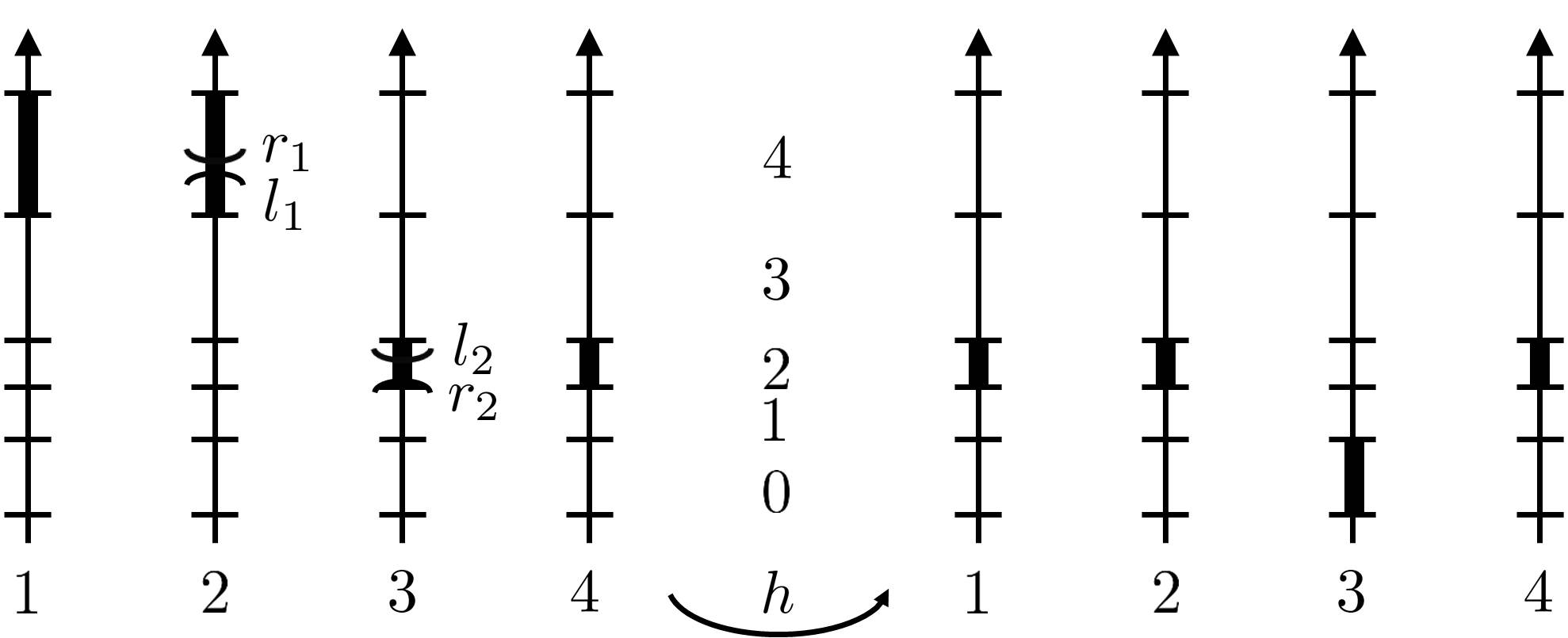
Figure 4: Illustration of a transition from χ=(4,4,2,2)𝜒4422\chi=(4,4,2,2) to ψ=(2,2,0,2)𝜓2202\psi=(2,2,0,2) in Ex. 4.2. The left side shows the preimage, the right the image state. The horizontal numbers correspond to the respective sites, while the vertical numbers display E={0,,4}𝐸04E=\{0,...,4\}. The states χ𝜒\chi and ψ𝜓\psi are marked by black rectangles at the corresponding sites.
Example 4.2.

This example shows that transitions at different sites are not independent in general. By comparing one CPA time step to one time step with the discretized FPO we see that a specific local transition at one site cannot take place if another specific local transition happens at a neighboring site, although both transitions are allowed locally. Consider I={1,,4}𝐼14I=\{1,...,4\}, and the system on dynamically invariant state space Ωm=[0,1]4superscriptΩ𝑚superscript014\Omega^{m}=[0,1]^{4} given for all n𝑛n\in\mathbb{N} by vin+1=h(vin,vi+1n)=vin+vi+1n3.75superscriptsubscript𝑣𝑖𝑛1superscriptsubscript𝑣𝑖𝑛superscriptsubscript𝑣𝑖1𝑛superscriptsubscript𝑣𝑖𝑛superscriptsubscript𝑣𝑖1𝑛3.75v_{i}^{n+1}=h(v_{i}^{n},v_{i+1}^{n})=\frac{v_{i}^{n}+v_{i+1}^{n}}{3.75} for i{1,,m1}𝑖1𝑚1i\in\{1,...,m-1\}. We have U={0,1}𝑈01U=\{0,1\} and define 555 intervals

Ωj=[wj,wj+1), for j{0,,3},Ω4=[w4,w5]formulae-sequencesubscriptΩ𝑗subscript𝑤𝑗subscript𝑤𝑗1formulae-sequence for 𝑗03subscriptΩ4subscript𝑤4subscript𝑤5\Omega_{j}=[w_{j},w_{j+1}),\quad\text{ for }j\in\{0,...,3\},\quad\Omega_{4}=[w_{4},w_{5}]

with

w0=0,w1=0.183,w2=0.31,w3=0.4,w4=0.7,w5=1,formulae-sequencesubscript𝑤00formulae-sequencesubscript𝑤10.183formulae-sequencesubscript𝑤20.31formulae-sequencesubscript𝑤30.4formulae-sequencesubscript𝑤40.7subscript𝑤51w_{0}=0,\quad w_{1}=0.183,\quad w_{2}=0.31,\quad w_{3}=0.4,\quad w_{4}=0.7,\quad w_{5}=1,

name them by their index and obtain a partition of ΩΩ\Omega with E={0,,4}𝐸04E=\{0,...,4\}, see Fig. 4. The induced flow is denoted by Φ1superscriptΦ1\Phi^{1} for one time step. We consider the CPA with V=U𝑉𝑈V=U for deterministic input gDBC(EI)𝑔subscript𝐷𝐵𝐶superscript𝐸𝐼g\in D_{BC}(E^{I}) given by g(φ)=δχ,φ𝑔𝜑subscript𝛿𝜒𝜑g(\varphi)=\delta_{\chi,\varphi}, where χ=(4,4,2,2)EI𝜒4422superscript𝐸𝐼\chi=(4,4,2,2)\in E^{I}. We focus on the image state ψ=(2,2,0,2)EI𝜓2202superscript𝐸𝐼\psi=(2,2,0,2)\in E^{I} and determine

l1=0.8,l2=0.3625,r1=0.83875,r2=0.32375formulae-sequencesubscript𝑙10.8formulae-sequencesubscript𝑙20.3625formulae-sequencesubscript𝑟10.83875subscript𝑟20.32375l_{1}=0.8,\quad l_{2}=0.3625,\quad r_{1}=0.83875,\quad r_{2}=0.32375

as the solution of the equations

h(w4,l1)=w3,h(l1,l2)=w2,h(r1,r2)=w2,h(r2,w2)=w1.formulae-sequencesubscript𝑤4subscript𝑙1subscript𝑤3formulae-sequencesubscript𝑙1subscript𝑙2subscript𝑤2formulae-sequencesubscript𝑟1subscript𝑟2subscript𝑤2subscript𝑟2subscript𝑤2subscript𝑤1h(w_{4},l_{1})=w_{3},\quad h(l_{1},l_{2})=w_{2},\quad h(r_{1},r_{2})=w_{2},\quad h(r_{2},w_{2})=w_{1}.

It is possible to show that

{Ωχ|1+U+VΦ1(Ωψ|1+V)}subscriptΩevaluated-at𝜒1𝑈𝑉superscriptΦ1subscriptΩevaluated-at𝜓1𝑉\displaystyle\{\Omega_{\chi|_{1+U+V}}\cap\Phi^{-1}(\Omega_{\psi|_{1+V}})\} {vΩ|w4v2l1,l2v3w3},absentconditional-set𝑣Ωformulae-sequencesubscript𝑤4subscript𝑣2subscript𝑙1subscript𝑙2subscript𝑣3subscript𝑤3\displaystyle\subseteq\{v\in\Omega\,|\,w_{4}\leq v_{2}\leq l_{1},l_{2}\leq v_{3}\leq w_{3}\},
{Ωσ1(χ|2+U+V)Φ1(Ωσ1(ψ|2+V))}subscriptΩsubscript𝜎1evaluated-at𝜒2𝑈𝑉superscriptΦ1subscriptΩsubscript𝜎1evaluated-at𝜓2𝑉\displaystyle\{\Omega_{\sigma_{1}(\chi|_{2+U+V})}\cap\Phi^{-1}(\Omega_{\sigma_{1}(\psi|_{2+V})})\} {vΩ|r1v21,w2v3r2},absentconditional-set𝑣Ωformulae-sequencesubscript𝑟1subscript𝑣21subscript𝑤2subscript𝑣3subscript𝑟2\displaystyle\subseteq\{v\in\Omega\,|\,r_{1}\leq v_{2}\leq 1,w_{2}\leq v_{3}\leq r_{2}\},

f0(σ1(χ|1+U+V))(σ1(ψ|1+V)))>0f_{0}(\sigma_{1}(\chi|_{1+U+V}))(\sigma_{1}(\psi|_{1+V})))>0 and f0(σ2(χ|2+U+V))(σ2(ψ|2+V))>0subscript𝑓0subscript𝜎2evaluated-at𝜒2𝑈𝑉subscript𝜎2evaluated-at𝜓2𝑉0f_{0}(\sigma_{2}(\chi|_{2+U+V}))(\sigma_{2}(\psi|_{2+V}))>0. Hence α^fβ^(g)(ψ)>0^𝛼𝑓^𝛽𝑔𝜓0\hat{\alpha}f\hat{\beta}(g)(\psi)>0, but

PB(g)(ψ)subscript𝑃𝐵𝑔𝜓\displaystyle P_{B}(g)(\psi) =φEIg(φ)PB,φ,ψ=λ(ΩχΦ1(Ωψ))λ(Ωχ)absentsubscript𝜑superscript𝐸𝐼𝑔𝜑subscript𝑃𝐵𝜑𝜓𝜆subscriptΩ𝜒superscriptΦ1subscriptΩ𝜓𝜆subscriptΩ𝜒\displaystyle=\sum_{\varphi\in E^{I}}g(\varphi)P_{B,\varphi,\psi}=\frac{\lambda(\Omega_{\chi}\cap\Phi^{-1}(\Omega_{\psi}))}{\lambda(\Omega_{\chi})}
\displaystyle\leq λ((Ωχ|1+U+VΦ1(Ωψ|1+V))(Ωχ|2+U+VΦ1(Ωψ|2+V)))λ(Ωχ)𝜆subscriptΩevaluated-at𝜒1𝑈𝑉superscriptΦ1subscriptΩevaluated-at𝜓1𝑉subscriptΩevaluated-at𝜒2𝑈𝑉superscriptΦ1subscriptΩevaluated-at𝜓2𝑉𝜆subscriptΩ𝜒\displaystyle\frac{\lambda((\Omega_{\chi|_{1+U+V}}\cap\Phi^{-1}(\Omega_{\psi|_{1+V}}))\cap(\Omega_{\chi|_{2+U+V}}\cap\Phi^{-1}(\Omega_{\psi|_{2+V}})))}{\lambda(\Omega_{\chi})}
=\displaystyle= λ()λ(Ωχ)=0,𝜆𝜆subscriptΩ𝜒0\displaystyle\frac{\lambda(\emptyset)}{\lambda(\Omega_{\chi})}=0,

and so α^fβ^(g)PB(g)^𝛼𝑓^𝛽𝑔subscript𝑃𝐵𝑔\hat{\alpha}f\hat{\beta}(g)\neq P_{B}(g).

Both examples are scalable in the sense that we can find analogous partitions of [0,c],c(0,1),0𝑐𝑐01[0,c],c\in(0,1), with the above properties by dividing all phase space coordinates by c𝑐c and complete the partition in [c,1]𝑐1[c,1] arbitrarily. So for decreasing size of the coding domains we can still find a partition of [0,1]01[0,1] with the above effects: locality errors are independent from resolution errors.

Furthermore the examples suggest to choose large V𝑉V for good approximations. Accordingly it can be proven that for maximal V𝑉V the CPA exactly corresponds to the discretized FPO.

Proposition 4.4.

For V=Vmax𝑉subscript𝑉V=V_{\max} we find that α^fβ^=PB^𝛼𝑓^𝛽subscript𝑃𝐵\hat{\alpha}f\hat{\beta}=P_{B}.

4.3 Consistency Theorem

The preceding results can be composed to a consistency result for uncertainty propagation with CPA: Up to technical postprocessing time evolution of probability densities with CPA can approximate time evolution with the FPO arbitrarily close.

Corollary 4.5.

Let T:ΩE:𝑇Ω𝐸T:\Omega\to E be a uniform partition with resolution ΔΩΔΩ\Delta\Omega and gκB1(DBC(EI))𝑔superscriptsubscript𝜅𝐵1subscript𝐷𝐵𝐶superscript𝐸𝐼g\in\kappa_{B}^{-1}(D_{BC}(E^{I})). Then

limΔΩ0limVVmaxκB1α^fβ^κB(g)PΦτ(g)1=0.subscriptΔΩ0subscript𝑉subscript𝑉𝑚𝑎𝑥subscriptnormsuperscriptsubscript𝜅𝐵1^𝛼𝑓^𝛽subscript𝜅𝐵𝑔subscript𝑃superscriptΦ𝜏𝑔10\lim_{\Delta\Omega\to 0}\lim_{V\to V_{max}}\|\kappa_{B}^{-1}\hat{\alpha}f\hat{\beta}\kappa_{B}(g)-P_{\Phi^{\tau}}(g)\|_{1}=0.

Proof Because there is only a finite number of possible V𝑉V, the limit VVmax𝑉subscript𝑉V\to V_{\max} is taken in the discrete topology. So the limit point is the evaluation with Vmaxsubscript𝑉V_{\max}, and Prop. 4.4 can be used. In a second step Thm. 4.2 can be applied to PΦτ(g)subscript𝑃superscriptΦ𝜏𝑔P_{\Phi^{\tau}}(g):

limΔΩ0limVVmaxκB1α^fβ^κB(g)PΦτ(g)1subscriptΔΩ0subscript𝑉subscript𝑉𝑚𝑎𝑥subscriptnormsuperscriptsubscript𝜅𝐵1^𝛼𝑓^𝛽subscript𝜅𝐵𝑔subscript𝑃superscriptΦ𝜏𝑔1\displaystyle\lim_{\Delta\Omega\to 0}\lim_{V\to V_{max}}\|\kappa_{B}^{-1}\hat{\alpha}f\hat{\beta}\kappa_{B}(g)-P_{\Phi^{\tau}}(g)\|_{1}
=\displaystyle= limΔΩ0limVVmaxκB1α^fβ^κB(g)PΦτ(g)1subscriptΔΩ0subscriptnormsubscript𝑉subscript𝑉superscriptsubscript𝜅𝐵1^𝛼𝑓^𝛽subscript𝜅𝐵𝑔subscript𝑃superscriptΦ𝜏𝑔1\displaystyle\lim_{\Delta\Omega\to 0}\|\lim_{V\to V_{\max}}\kappa_{B}^{-1}\hat{\alpha}f\hat{\beta}\kappa_{B}(g)-P_{\Phi^{\tau}}(g)\|_{1}
=\displaystyle= limΔΩ0RPΦτ(g)PΦτ(g)1subscriptΔΩ0subscriptnorm𝑅subscript𝑃superscriptΦ𝜏𝑔subscript𝑃superscriptΦ𝜏𝑔1\displaystyle\lim_{\Delta\Omega\to 0}\|RP_{\Phi^{\tau}}(g)-P_{\Phi^{\tau}}(g)\|_{1}
=\displaystyle= 0.0\displaystyle 0.\qquad\qed

5 Example

In this section we comment on how to implement an algorithm to evolve uncertainties with CPA. The algorithm is tested at the problem of arsenate transportation and asorption in drinking water pipes, and the results are compared to a Monte Carlo calculation. Although the theory has been developed for uncertainties in initial conditions, in this applicational part we extend the concept slightly such that CPA can cope with certain stochastic boundary conditions. This is important in contaminant transport modeling [43]. With this first generalization we want to provide evidence that with CPA the treatment of more general stochastic spatio-temporal processes seems feasible.

5.1 Stochastic Boundary Conditions

We deal with stationary temporal white noise boundary conditions

glD(EKl)subscript𝑔𝑙𝐷superscript𝐸subscript𝐾𝑙\displaystyle g_{l}\in D(E^{K_{l}}) for Kl={1,,r},for subscript𝐾𝑙1𝑟\displaystyle\text{ for }K_{l}=\{1,...,r\},
grD(EKr)subscript𝑔𝑟𝐷superscript𝐸subscript𝐾𝑟\displaystyle g_{r}\in D(E^{K_{r}}) for Kr={ms+1,,m}for subscript𝐾𝑟𝑚𝑠1𝑚\displaystyle\text{ for }K_{r}=\{m-s+1,...,m\}

instead of deterministic ρEK𝜌superscript𝐸𝐾\rho\in E^{K}. With stationary we mean that the densities do not change in time, and the term temporal white noise indicates that there are no correlations in the boundary random variable’s realizations at different times.

For this purpose the global function in Def. 3.9 is extendend to

f:DdBeI~DdBeI~,gf(g),:𝑓formulae-sequencesuperscriptsubscript𝐷𝑑𝐵𝑒~𝐼superscriptsubscript𝐷𝑑𝐵𝑒~𝐼maps-to𝑔𝑓𝑔f:D_{dBe}^{\tilde{I}}\rightarrow D_{dBe}^{\tilde{I}},\quad g\mapsto f(g),
g¯(i)(φ)¯𝑔𝑖𝜑\displaystyle\underline{g}(i)(\varphi) =σil(φ)|{1,,r+ili}χEKl s.t. σiil(χ)|{1,,r+ili}=gl(χ),absentsubscript𝜒evaluated-atsuperscript𝐸subscript𝐾𝑙 s.t. subscript𝜎𝑖subscript𝑖𝑙𝜒1𝑟subscript𝑖𝑙𝑖absentevaluated-atsubscript𝜎subscript𝑖𝑙𝜑1𝑟subscript𝑖𝑙𝑖subscript𝑔𝑙𝜒\displaystyle=\sum_{\overset{\chi\in E^{K_{l}}\text{ s.t. }\sigma_{i-i_{l}}(\chi)|_{\{1,...,r+i_{l}-i\}}=}{\sigma_{-i_{l}}(\varphi)|_{\{1,...,r+i_{l}-i\}}}}g_{l}(\chi),
g¯(i)(φ)¯𝑔𝑖𝜑\displaystyle\overline{g}(i)(\varphi) =σir(φ)|{ms+1i+ir,,m}χEKr s.t. σiir(χ)|{ms+1i+ir,,m}=gr(χ),absentsubscript𝜒evaluated-atsuperscript𝐸subscript𝐾𝑟 s.t. subscript𝜎𝑖subscript𝑖𝑟𝜒𝑚𝑠1𝑖subscript𝑖𝑟𝑚absentevaluated-atsubscript𝜎subscript𝑖𝑟𝜑𝑚𝑠1𝑖subscript𝑖𝑟𝑚subscript𝑔𝑟𝜒\displaystyle=\sum_{\overset{\chi\in E^{K_{r}}\text{ s.t. }\sigma_{i-i_{r}}(\chi)|_{\{m-s+1-i+i_{r},...,m\}}=}{\sigma_{-i_{r}}(\varphi)|_{\{m-s+1-i+i_{r},...,m\}}}}g_{r}(\chi),
f(g)(i)(ψ)𝑓𝑔𝑖𝜓\displaystyle f(g)(i)(\psi) =φEU+Vg¯(i)(φ)αU~(i)(σi(g)|U~(i))(φ|V+U~(i))g¯(i)(φ)f0(φ)(ψ).absentsubscript𝜑superscript𝐸𝑈𝑉¯𝑔𝑖𝜑subscript𝛼~𝑈𝑖evaluated-atsubscript𝜎𝑖𝑔~𝑈𝑖evaluated-at𝜑𝑉~𝑈𝑖¯𝑔𝑖𝜑subscript𝑓0𝜑𝜓\displaystyle=\sum_{\varphi\in E^{U+V}}\underline{g}(i)(\varphi)\cdot\alpha_{\tilde{U}(i)}(\sigma_{i}(g)|_{\tilde{U}(i)})(\varphi|_{V+\tilde{U}(i)})\cdot\overline{g}(i)(\varphi)\cdot f_{0}(\varphi)(\psi).

Furthermore the relations between global and de Bruijn densities then have to be generalized to α^:D(EKl)×DdBeI~×D(EKr)D(EI),(gl×g×gr)α^((gl×g×gr)):^𝛼formulae-sequence𝐷superscript𝐸subscript𝐾𝑙superscriptsubscript𝐷𝑑𝐵𝑒~𝐼𝐷superscript𝐸subscript𝐾𝑟𝐷superscript𝐸𝐼maps-tosubscript𝑔𝑙𝑔subscript𝑔𝑟^𝛼subscript𝑔𝑙𝑔subscript𝑔𝑟\hat{\alpha}:D(E^{K_{l}})\times D_{dBe}^{\tilde{I}}\times D(E^{K_{r}})\to D(E^{I}),\,(g_{l}\times g\times g_{r})\mapsto\hat{\alpha}((g_{l}\times g\times g_{r})) with

α^((gl×g×gr))(ψ)^𝛼subscript𝑔𝑙𝑔subscript𝑔𝑟𝜓\displaystyle\hat{\alpha}((g_{l}\times g\times g_{r}))(\psi) =gl(ψ|Kl)αI~(g)(ψ|{1+r,,ms})gr(ψ|Kr)absentsubscript𝑔𝑙evaluated-at𝜓subscript𝐾𝑙subscript𝛼~𝐼𝑔evaluated-at𝜓1𝑟𝑚𝑠subscript𝑔𝑟evaluated-at𝜓subscript𝐾𝑟\displaystyle=g_{l}(\psi|_{K_{l}})\alpha_{\tilde{I}}(g)(\psi|_{\{1+r,...,m-s\}})g_{r}(\psi|_{K_{r}})

and β^:D(EI)D(EKl)×DdBeI~×D(EKr),gβ^(g)=(gl,gI~,gr):^𝛽formulae-sequence𝐷superscript𝐸𝐼𝐷superscript𝐸subscript𝐾𝑙superscriptsubscript𝐷𝑑𝐵𝑒~𝐼𝐷superscript𝐸subscript𝐾𝑟maps-to𝑔^𝛽𝑔subscript𝑔𝑙subscript𝑔~𝐼subscript𝑔𝑟\hat{\beta}:D(E^{I})\to D(E^{K_{l}})\times D_{dBe}^{\tilde{I}}\times D(E^{K_{r}}),\,g\mapsto\hat{\beta}(g)=(g_{l},g_{\tilde{I}},g_{r}) with

gl(ψ)subscript𝑔𝑙𝜓\displaystyle g_{l}(\psi) =χEI s. t. χ|Kr=ψg(χ),absentsubscript𝜒evaluated-atsuperscript𝐸𝐼 s. t. 𝜒subscript𝐾𝑟𝜓𝑔𝜒\displaystyle=\sum_{\chi\in E^{I}\text{ s. t. }\chi|_{K_{r}}=\psi}g(\chi),
gI~(i)(ψ)subscript𝑔~𝐼𝑖𝜓\displaystyle g_{\tilde{I}}(i)(\psi) =χ|i+V=σi(ψ)χEI s. t. g(χ),absentsubscript𝜒superscript𝐸𝐼 s. t. evaluated-at𝜒𝑖𝑉subscript𝜎𝑖𝜓𝑔𝜒\displaystyle=\sum_{\overset{\chi\in E^{I}\text{ s. t. }}{\chi|_{i+V}=\sigma_{-i}(\psi)}}g(\chi),
gr(ψ)subscript𝑔𝑟𝜓\displaystyle g_{r}(\psi) =χEI s. t. χ|Kl=ψg(χ).absentsubscript𝜒evaluated-atsuperscript𝐸𝐼 s. t. 𝜒subscript𝐾𝑙𝜓𝑔𝜒\displaystyle=\sum_{\chi\in E^{I}\text{ s. t. }\chi|_{K_{l}}=\psi}g(\chi).

CPA with stochastic boundary conditions may be used to approximate spatio-temporal processes with deterministic dynamics, in which the initial and boundary conditions are stochastic. We remark that it is straight-forward to use time-dependent stochastic boundary conditions instead of stationary ones.

5.2 Implementation

From an implementational point of view two steps of uncertainty propagation with CPA have to be distinguished. Step one is the tranlation of the completely continuous system into a CPA. This is independent of initial or boundary conditions and can be achieved in a preprocessing procedure. Step two consists of the CPA evolution with given initial and boundary values. It turns out that step one is numerically more expensive than step two. For industrial applications like simulation based system monitoring the CPA method points towards real-time uncertainty quantification, because the slow step one only has to be performed once before the actual simulation. We furthermore note that by construction the simulation is parallelizable in space.

Step one basically consists of the approximation of local transition probabilities. We propose a local version of the standard Monte Carlo quadrature approach [18] in set oriented numerics for this purpose. We remark that also advanced adaptive methods have been suggested, see e. g. [13].

  • i)

    For φEU+V𝜑superscript𝐸𝑈𝑉\varphi\in E^{U+V} choose Wφsubscript𝑊𝜑W_{\varphi} test vectors wi=(wi,rp,,wi,s+q)(n)U+Vsubscript𝑤𝑖subscript𝑤𝑖𝑟𝑝subscript𝑤𝑖𝑠𝑞superscriptsuperscript𝑛𝑈𝑉w_{i}=(w_{i,-r-p},...,w_{i,s+q})\in(\mathbb{R}^{n})^{U+V}, where {wi,j}iWφsubscriptsubscript𝑤𝑖𝑗𝑖subscript𝑊𝜑\{w_{i,j}\}_{i\leq W_{\varphi}} is randomly distributed over coding domain Ωφ(j)ΩsubscriptΩ𝜑𝑗Ω\Omega_{\varphi(j)}\subseteq\Omega, respectively.

  • ii)

    Compute for all iWφ𝑖subscript𝑊𝜑i\leq W_{\varphi} the image points

    w~i=(h(τ,wi,rp,,wi,sp),h(τ,wi,rp+1,,wi,sp+1),,h(τ,wi,r+q,,wi,s+q)).subscript~𝑤𝑖𝜏subscript𝑤𝑖𝑟𝑝subscript𝑤𝑖𝑠𝑝𝜏subscript𝑤𝑖𝑟𝑝1subscript𝑤𝑖𝑠𝑝1𝜏subscript𝑤𝑖𝑟𝑞subscript𝑤𝑖𝑠𝑞\tilde{w}_{i}=(h(\tau,w_{i,-r-p},...,w_{i,s-p}),h(\tau,w_{i,-r-p+1},...,w_{i,s-p+1}),...,h(\tau,w_{i,-r+q},...,w_{i,s+q})).
  • iii)

    Determine ψ1,,ψLEVsubscript𝜓1subscript𝜓𝐿superscript𝐸𝑉\psi_{1},...,\psi_{L}\in E^{V} such that there is lL𝑙𝐿l\leq L and w~isubscript~𝑤𝑖\tilde{w}_{i} with T((w~i)j)=(ψl)j𝑇subscriptsubscript~𝑤𝑖𝑗subscriptsubscript𝜓𝑙𝑗T((\tilde{w}_{i})_{j})=(\psi_{l})_{j} for all jV𝑗𝑉j\in V. Let the number of image points in the specific coding domain be denoted by Wψlsubscript𝑊subscript𝜓𝑙W_{\psi_{l}}, i.e. l=1LWψl=Wφsuperscriptsubscript𝑙1𝐿subscript𝑊subscript𝜓𝑙subscript𝑊𝜑\sum_{l=1}^{L}W_{\psi_{l}}=W_{\varphi}. The local transition function is then approximated by

    f0(φ)(ψ)={Wψ/Wφ for all ψ{ψ1,,ψL}0 else .subscript𝑓0𝜑𝜓casessubscript𝑊𝜓subscript𝑊𝜑 for all 𝜓subscript𝜓1subscript𝜓𝐿0 else f_{0}(\varphi)(\psi)=\left\{\begin{array}[]{ll}W_{\psi}/W_{\varphi}&\mbox{ for all }\psi\in\{\psi_{1},...,\psi_{L}\}\\ 0&\mbox{ else }\\ \end{array}\right..

With increasing number of test points the approximation is expected to get better. However, the number of evaluations grows exponentially in |V|𝑉|V|. So we suggest to use de Bruijn calculus to determine transition probabilities for large V𝑉V from transition probabilities for smaller V~~𝑉\tilde{V}, see Fig. 3. For given f~0:EU+V~D(EV~):subscript~𝑓0superscript𝐸𝑈~𝑉𝐷superscript𝐸~𝑉\tilde{f}_{0}:E^{U+\tilde{V}}\to D(E^{\tilde{V}}) and W𝑊W given by V=V~+W𝑉~𝑉𝑊V=\tilde{V}+W

f0:EV+UD(EV),φf0(φ),:subscript𝑓0formulae-sequencesuperscript𝐸𝑉𝑈𝐷superscript𝐸𝑉maps-to𝜑subscript𝑓0𝜑f_{0}:E^{V+U}\to D(E^{V}),\quad\varphi\mapsto f_{0}(\varphi),

where

f0(φ)(ψ)=αW(g^)(ψ),subscript𝑓0𝜑𝜓subscript𝛼𝑊^𝑔𝜓f_{0}(\varphi)(\psi)=\alpha_{W}(\hat{g})(\psi),
g^(D(EV~))W,g^(i)=f~0(φ|i+V~+U).formulae-sequence^𝑔superscript𝐷superscript𝐸~𝑉𝑊^𝑔𝑖subscript~𝑓0evaluated-at𝜑𝑖~𝑉𝑈\hat{g}\in(D(E^{\tilde{V}}))^{W},\quad\hat{g}(i)=\tilde{f}_{0}(\varphi|_{i+\tilde{V}+U}).

It can be shown with an example similar to Ex. 4.2 that this is again just an approximation of the directly calculated f0subscript𝑓0f_{0}.

Regarding step two, the simulation with CPA, we remark that it is important to only follow and store states with probability larger than a specified threshold whenever possible. Otherwise already for reasonably large E𝐸E or V𝑉V the calculations are not feasible. An example is the de Bruijn density DdBeI~superscriptsubscript𝐷𝑑𝐵𝑒~𝐼D_{dBe}^{\tilde{I}}, where |E||V|superscript𝐸𝑉|E|^{|V|} numbers would have to be handled at every site in I~~𝐼\tilde{I}. The set of states with positive probability is much smaller, although it typically first grows and then shrinks again in the transient phase of dynamics. Note that our de Bruijn choice of αWsubscript𝛼𝑊\alpha_{W} enables such sparse calculations, whereas the whole space is needed to solve for example a linear nonnegative least squares problem.

5.3 Arsenate Fate in Water Pipe

Consider the advection and adsorption of arsenate in drinking water pipes, a topic that has attracted a lot of attention in the water supply community lately [38, 25]. We describe a water tank on a hill and a pipe to a consumer in a valley. Report locations to observe the arsenate concentrations are installed in a distance of ΔxΔ𝑥\Delta x, see Fig. 5a. The physics is described by the Langmuir adsorption model [27]

tD+vxD=1rh11k1+1kf(SmaxA)(D(SmaxA)KeqA),tA=11k1+1kf(SmaxA)(D(SmaxA)KeqA)formulae-sequencesubscript𝑡𝐷𝑣subscript𝑥𝐷1subscript𝑟11subscript𝑘11subscript𝑘𝑓subscript𝑆𝑚𝑎𝑥𝐴𝐷subscript𝑆𝑚𝑎𝑥𝐴subscript𝐾𝑒𝑞𝐴subscript𝑡𝐴11subscript𝑘11subscript𝑘𝑓subscript𝑆𝑚𝑎𝑥𝐴𝐷subscript𝑆𝑚𝑎𝑥𝐴subscript𝐾𝑒𝑞𝐴\begin{split}\partial_{t}D+v\partial_{x}D&=-\frac{1}{r_{h}}\frac{1}{\frac{1}{k_{1}}+\frac{1}{k_{f}}(S_{max}-A)}(D(S_{max}-A)-K_{eq}A),\\ \partial_{t}A&=\frac{1}{\frac{1}{k_{1}}+\frac{1}{k_{f}}(S_{max}-A)}(D(S_{max}-A)-K_{eq}A)\end{split}

where D𝐷D is the concentration of dissolved arsenate in mgl𝑚𝑔𝑙\frac{mg}{l} and A𝐴A the concentration of arsenate adsorbed at the pipe wall in mgm2𝑚𝑔superscript𝑚2\frac{mg}{m^{2}}. We adopt realistic parameter values from [25, 36]

v𝑣\displaystyle v =10mmin,absent10𝑚𝑚𝑖𝑛\displaystyle=10\frac{m}{min}, rhsubscript𝑟\displaystyle r_{h} =50lm2,absent50𝑙superscript𝑚2\displaystyle=50\frac{l}{m^{2}},
k1subscript𝑘1\displaystyle k_{1} =0.2lmgmin,absent0.2𝑙𝑚𝑔𝑚𝑖𝑛\displaystyle=0.2\frac{l}{mg\,min}, Smaxsubscript𝑆𝑚𝑎𝑥\displaystyle S_{max} =100mgm2,absent100𝑚𝑔superscript𝑚2\displaystyle=100\frac{mg}{m^{2}},
Keqsubscript𝐾𝑒𝑞\displaystyle K_{eq} =0.0537mgl,absent0.0537𝑚𝑔𝑙\displaystyle=0.0537\frac{mg}{l}, kfsubscript𝑘𝑓\displaystyle k_{f} =2.4lm2min,absent2.4𝑙superscript𝑚2𝑚𝑖𝑛\displaystyle=2.4\frac{l}{m^{2}\,min},

and consider the system on the approximately positively invariant ΩΩ\Omega given by D[0,1]𝐷01D\in[0,1] and A[0,Smax]𝐴0subscript𝑆𝑚𝑎𝑥A\in[0,S_{max}]. The backward difference with U={1,0}𝑈10U=\{-1,0\}, Δx=100mΔ𝑥100𝑚\Delta x=100m and Δt=Δx/v=10minΔ𝑡Δ𝑥𝑣10𝑚𝑖𝑛\Delta t=\Delta x/v=10min is used.

Refer to caption
(a)
Refer to caption
(b)
Refer to caption
(c)
Refer to caption
(d)
Refer to caption
(e)
Figure 5: (a) A reservoir on a hill is connected to a consumer in a valley through a pipe with 6 report locations. (b) The phase space at every report location is divided into 5×5555\times 5 coding domains, and the steady states are drawn in green. For example f0(((1,4),(2,4)))subscript𝑓01424f_{0}(((1,4),(2,4))) can be approximated by the transition of blue test points in domain (1,4)14(1,4) and black ones in domain (2,4)24(2,4) to the set of red points. (c) shows the initial conditions for an exemplary simulation with the according CPA, and the results after 1 and 7 hours are shown in (d) and (e), respectively. See also Fig. 6.

To obtain the local function of a CPA we map test points by using intermediate steps on the basis of the method of characteristics with the smaller Δt=0.1minΔsuperscript𝑡0.1𝑚𝑖𝑛\Delta t^{\prime}=0.1min and Δx=1mΔsuperscript𝑥1𝑚\Delta x^{\prime}=1m. We use V=V~={0}𝑉~𝑉0V=\tilde{V}=\{0\} and partition the phase space equidistantly with 5 symbols in each of the n=2𝑛2n=2 directions. If we label the coding domains from 00 to 444 in each direction, the corresponding CPA results from transition probabilities like

f0(((1,4),(2,4)))(ψ)={0.806 if ψ=(1,4)0.194 if ψ=(2,4)0 else ,subscript𝑓01424𝜓cases0.806 if 𝜓140.194 if 𝜓240 else f_{0}(((1,4),(2,4)))(\psi)=\left\{\begin{array}[]{ll}0.806&\mbox{ if }\psi=(1,4)\\ 0.194&\mbox{ if }\psi=(2,4)\\ 0&\mbox{ else }\\ \end{array}\right.,

see Fig. 5b. White noise boundary conditions are applied to describe a random arsenate source in the tank, and deterministic initial values represent a pipe which is completely empty in the beginning. The observed dynamics is shown in Fig. 5c-5e: Dissolved arsenate is transported along the pipe, and over time the walls are covered more and more with adsorbed arsenate. After 242424 hours a steady state is reached, and we compare it to a Monte Carlo calculation, see Fig. 6a-6b. The latter has also been obtained on the basis of the method of characteristics with Δt=0.1minΔsuperscript𝑡0.1𝑚𝑖𝑛\Delta t^{\prime}=0.1min and Δx=1mΔsuperscript𝑥1𝑚\Delta x^{\prime}=1m for 200002000020000 evaluations. The boundary condition has been drawn from the stationary boundary distribution every 10min10𝑚𝑖𝑛10min and held constant in the meantime. Our example features an interesting probabilitic effect due to the nonlinearity of the reaction equations. Although the boundary values are distributed in the D𝐷D-domains 24242-4, the consumer mostly observes dissolved arsenate at a concentration of domain 444 in the steady state.

Refer to caption
(a)
Refer to caption
(b)
Refer to caption
(c)
Refer to caption
(d)
Figure 6: Steady states after 242424 hours. (a) shows the result of a Monte Carlo computation. In (b) one finds the result for a CPA with a state space resolution of 5×5555\times 5 and pattern size V~=V={0}~𝑉𝑉0\tilde{V}=V=\{0\}, in (c) the results for 5×155155\times 15 and V~=V={0}~𝑉𝑉0\tilde{V}=V=\{0\}, and in (d) the ones for 5×5555\times 5 and V~={0},V={1,0}formulae-sequence~𝑉0𝑉10\tilde{V}=\{0\},V=\{-1,0\}.

Furthermore we plot the steady state results from CPA for which the approximation parameters are altered. In Fig. 6c the result is plotted for V~=V={0}~𝑉𝑉0\tilde{V}=V=\{0\} with an equidistant phase space partition of 555 domains in D𝐷D- and 151515 domains in A𝐴A-direction, whereas in Fig. 6d the pattern size is extended by W={1,0}𝑊10W=\{-1,0\} to V={1,0}𝑉10V=\{-1,0\}. It is observed that in this example increasing the pattern size does not improve the result if compared to the Monte Carlo case, but increasing the state space resolution has a notable effect. In all cases we used 75 test points for the coding domain at site 00 and 37 at site 11-1 to approximate the local function, and a probability threshold of 0.000050.000050.00005 in the simulation.

We note that there is often no interest in global results and accordingly no need to transform between local and fully global states with α^^𝛼\hat{\alpha}. Local information like indicated in the graphs can be directly extracted from the CPA result. Similarly, in practice the information about initial values is often given locally, such that there is no need to use the full β^^𝛽\hat{\beta}. Besides, we note that the discrete state space information is often completely sufficient in practice. In the example a consumer is interested rather in risk level or threshold information about water contamination than in information in form of exact concentrations. In some biological sytems even the Boolean case, |E|=2𝐸2|E|=2, is enough [3].

6 Conclusion

We have introduced a numerical scheme for density based uncertainty propagation in certain spatio-temporal systems. It consists of a preprocessing step, in which the underlying PDE system is translated into a cellular probabilistic automaton, and a simulation step, in which initial and boundary conditions are evolved. The simulation is parallelizable in the space extension and fast in relation to the preprocessing. Furthermore it computes on discrete states instead of on the continuous phase space. Because the discrete states can be interpreted as risk levels, fast uncertainty propagation directly on this simplified state space suites industrial demands.

The algorithm is based on state space discretization like in set oriented numerics and on the de Bruijn state idea from cellular automata theory. There are two parameters that allow to control the approximation of the exact density evolution: state space resolution and de Bruijn pattern size. We have proven consistency of the method for uncertain initial conditions under deterministic dynamics and have paved the way towards the handling of spatio-temporal processes with more involved stochastic influence. More precisely, it has been shown how to deal with white noise boundary conditions, an important topic for example in contaminant transport modeling. However, it seems difficult to preserve temporal correlations in random parameters with our algorithm. Future research will focus on white noise parameters. We are confident that they only extend the preprocessing, whereas the simulation step is not changed. In this sense CPA promise to overcome the curse of dimension in parameter space. Besides, we want to investigate how our algorithm performs in more complex applications like the simulation of drinking or waste water grids.

7 Acknowledgements

The authors would like to thank Birgit Obst from Siemens Corporate Technology for helpful discussions about the arsenate example.

References

  • [1] F. Augustin and P. Rentrop, Stochastic Galerkin techniques for random ordinary differential equations, Numer. Math., (2012), pp. 1–21.
  • [2] A. Barth, C. Schwab, and N. Zollinger, Multi-Level Monte Carlo Finite Element method for elliptic PDE’s with stochastic coefficients, ETH Zürich, Research Report, 2010-18 (2010).
  • [3] M. Davidich and S. Bornholdt, The transition from differential equations to Boolean networks: A case study in simplifying a regulatory network model., J. Theor. Biol., 255 (2008), pp. 269–277.
  • [4] M. Dellnitz and O. Junge, On the Approximation of Complicated Dynamical Behavior, SIAM J. Numer. Anal., 36 (1999), pp. 491–515.
  • [5]  , Set oriented numerical methods for dynamical systems, vol. 2 of Handbook of Dynamical Systems, Elsevier Science, 2002, pp. 221–264.
  • [6] A. Deutsch and S. Dormann, Cellular automaton modeling of biological pattern formation, Birkhäuser, Boston, MA, 2005.
  • [7] B. L. Fox, Strategies for Quasi-Monte Carlo, Kluwer Academic Publishers Group, Dordrecht, Netherlands, 1999.
  • [8] R. Ghanem and P. Spanos, Stochastic Finite Elements: A Spectral Approach, Springer-Verlag, New York, NY, 1991.
  • [9] A. L. Gibbs and F. E. Su, On choosing and bounding probability metrics, Internat. Statist. Rev., 70 (2002), pp. 419–435.
  • [10] W. R. Gilks, S. Richardson, and D. J. Spiegelhalter, Markov Chain Monte Carlo in practice, Chapman and Hall/CRC, Boca Raton, FL, 1995.
  • [11] L. Grüne and O. Junge, Global optimal control of perturbed systems, J. Optimiz. Theory App., 136 (2008), pp. 411–429.
  • [12] J. Guckenheimer and P. Holmes, Nonlinear Oscillations, Dynamical Systems, and Bifurcations of Vector Fields, Springer-Verlag, New York, NY, 1983.
  • [13] R. Guder, M. Dellnitz, and E. Kreuzer, An adaptive method for the approximation of the generalized cell mapping, Chaos, Soliton. Fract., 8 (1997), pp. 525–534.
  • [14] F. v. Haeseler, H.-O. Peitgen, and G. Skordev, Cellular automata, matrix substitutions and fractals, Ann. Math. Artif. Intel., 8 (1993), pp. 345–362.
  • [15] H. Hanche-Olsen and H. Holden, The Kolmogorov-Riesz compactness theorem, Expo. Math., 28 (2010), pp. 385–394.
  • [16] J. Hawkins and D. Molinek, One-dimensional stochastic cellular automata, Topol. P., 31 (2007), pp. 515–532.
  • [17] C. S. Hsu, Cell-to-Cell Mapping: A Method of Global Analysis for Nonlinear Systems, Springer, New York, NY, 1987.
  • [18] F. Y. Hunt, A Monte Carlo approach to the approximation of invariant measures, Random Comput. Dynam., 2 (1994), pp. 111–133.
  • [19] O. Junge, J. E. Marsden, and I. Mezić, Uncertainty in the dynamics of conservative maps, Proceedings of the 43rd IEEE Conference on Decision and Control, 2004.
  • [20] J. Kari, Theory of cellular automata: A survey, Theor. Comput. Sci., 334 (2005), pp. 3–33.
  • [21] G. E. Karniadakis, C. H. Su, D. Xiu, D. Lucor, C. Schwab, and R. A. Todor, Generalized polynomial chaos solution for differential equations with random inputs, ETH Zürich, Research Report, 2005-01 (2005).
  • [22] J. M. Keeling, The effects of local spatial structure on epidemiological invasions, Proc. R. Soc. Lond. B, 266 (1999), pp. 859–867.
  • [23] P. E. Kloeden and E. Platen, Numerical Solution of Stochastic Differential Equations, Springer, New York, NY, 2011.
  • [24] P. E. Kloeden, E. Platen, and H. Schurz, Numerical Solution of SDE through Computer Experiments, Springer, Berlin, Germany, 1994.
  • [25] S. Klostermann, R. Murray, J. Szabo, J. Hall, and J. Uber, Modeling and simulation of arsenate fate and transport in a distribution system simulator, in Proceedings of Water Distribution System Analysis, 2010.
  • [26] P. Koltai, Efficient approximation methods for the global long-term behavior of dynamical systems - Theory, algorithms and examples, PhD thesis, 2010.
  • [27] L. K. Koopal and M. J. Avena, A simple model for adsorption kinetics at charged solid-liquid interfaces, Colloid. Surface. A, 192 (2001), pp. 93–107.
  • [28] H. Kushner and P. Dupuis, Numerical Methods for Stochastic Control Problems in Continuous Time, Springer, New York, NY, 2001.
  • [29] H. P. Langtangen, Numerical solution of first passage problems in random vibrations, SIAM J. Sci. Comput., 15 (1994), pp. 977–996.
  • [30] A. Lasota and M. C. Mackey, Chaos, Fractals, and Noise: Stochastic Aspects of Dynamics, Springer, New York, NY, 1993.
  • [31] C. L. Lawson and R. J. Hanson, Solving least squares problems, Prentice-Hall, Englewood Cliffs, NJ, 1974.
  • [32] W. L. Loh, On Latin Hypercube Sampling, Ann. Stat., 24 (1996), pp. 2058–2080.
  • [33] R. E. Melchers, Structural Reliability Analysis and Prediction, John Wiley & Sons, Chichester, United Kingdom, 1999.
  • [34] I. Mezić and T. Runolfsson, Uncertainty propagation in dynamical systems, Automatica, 44 (2008), pp. 3003–3013.
  • [35] B. K. Oksendal, Stochastic Differential Equations: An Introduction with Applications, Springer, New York, NY, 2002.
  • [36] M. L. Pierce and C. B. Moore, Adsorption of arsenite and arsenate on amorphous iron hydroxide, Water Res., 16 (1982), pp. 1247–1253.
  • [37] A. Rössler, Runge-Kutta Methods for the strong approximation of solutions of stochastic differential equations, SIAM J. Numer. Anal., 48 (2010), pp. 922–952.
  • [38] F. Shang, J. G. Uber, L. A. Rossman, R. Janke, and R. Murray, EPANET Multi-Species Extension User’s Manual, US Environmental Protection Agency, Cincinatti, OH, 2011.
  • [39] K. Sutner, De Bruijn Graphs and Linear Cellular Automata, Complex Systems, 5 (1991), pp. 19–30.
  • [40] S. M. Ulam, A Collection of Mathematical Problems, Interscience Publisher, New York, NY, 1960.
  • [41] R. Vollmar, Algorithmen in Zellularautomaten, Teubner, Stuttgart, Germany, 1979.
  • [42] X. Wan and G. E. Karniadakis, Multi-element generalized polynomial chaos for arbitrary probability measures, SIAM J. Sci. Comput., 28 (2006), pp. 901–928.
  • [43] P. P. Wang and C. Zheng, Contaminant transport models under random sources, Ground water, 43 (2005), pp. 423–433.
  • [44] N. Wiener, The homogeneous chaos, Am. J. Math., 60 (1938), pp. 897–936.
  • [45] J. Wloka, Funktionalanalysis und Anwendungen, Walter de Gruyter, Berlin, Germany, 1971.