Using proper divergence functions to evaluate
climate models
Abstract
It has been argued persuasively that, in order to evaluate climate models, the probability distributions of model output need to be compared to the corresponding empirical distributions of observed data. Distance measures between probability distributions, also called divergence functions, can be used for this purpose. We contend that divergence functions ought to be proper, in the sense that acting on modelers’ true beliefs is an optimal strategy. Score divergences that derive from proper scoring rules are proper, with the integrated quadratic distance and the Kullback-Leibler divergence being particularly attractive choices. Other commonly used divergences fail to be proper. In an illustration, we evaluate and rank simulations from fifteen climate models for temperature extremes in a comparison to re-analysis data.
1 Introduction
Traditionally, climate models have been assessed by comparing summary statistics or point estimates that derive from the simulated model output to the corresponding observed quantities [1, 2]. However, there is a growing consensus that in order to evaluate climate models the probability distribution of model output needs to be compared to the corresponding distribution of observed data. Guttorp [3, p. 820] argues powerfully that
Climate models are difficult to compare to data. Often climatologists compute some summary statistic, such as global annual mean temperature, and compare climate models using observed (or rather estimated) forcings to the observed (or rather estimated) temperatures. However, it seems more appropriate to compare the distribution (over time and space) of climate model output to the corresponding distribution of observed data, as opposed to point estimates with or without confidence intervals.
Palmer [4, p. 850] and Arnold et al. [5] join this argument, by proposing the use of the Hellinger distance between simulated and observed probability distributions to assess climate models. A pioneering effort in these directions is that of Perkins et al. [6] who use a transportation type metric; however, this metric applies to densities only and thus requires density estimates.
Taking a broader perspective, predictive models are key tools in many realms of science and society, and principled methods for assessing their performance are in strong demand. Any such evaluation procedure ought to provide a quantitative assessment of the compatibility of the simulation model, and the real world phenomena it is meant to represent, in a manner that encourages careful assessment and integrity. In this paper, we focus on the setting in which the simulation model supplies a probability distribution, , typically consisting of model output composited over time and/or space, and we wish to evaluate it against the empirical measure, , associated with the corresponding observations. The evaluation then is usually performed by computing a distance measure or divergence, , between the probability distributions and , where the divergence function is such that and for all probability distributions and . Competing climate models give rise to distinct simulated probability distributions, and those that yield the smallest divergences when compared to the empirical measure are considered to perform best.
Myriads of distance measures for probability distributions have been studied in the literature, as reviewed comprehensively by Deza and Deza [7, Chapter 14] and Gibbs and Su [8], and it is far from obvious which ought to be used for evaluation purposes. Our paper aims to provide guidance in the choice of the divergence function in a general setting, including both categorical and continuous, real- or vector-valued observations. The task is not unique to climatology, and essentially the same problem arises in the emerging transdisciplinary field of uncertainty quantification. In this latter context, Ferson et al. [9, §5.2] list desirable properties of a divergence function in the case of a real-valued observation, in that444Ferson et al. [9, §5.2] furthermore request the unboundedness of the divergence function. We suppress this request, as the compatibility property (i) implies unboundedness.
-
(i)
the divergence between point measures and ought to reduce to the absolute error ;
-
(ii)
the divergence ought to be sensitive to all distributional facets, rather than just means and variances;
-
(iii)
the divergence ought to be expressible in physical units555For example, if we are concerned with temperature simulations in degrees Celsius, then the divergence should have a value in degrees Celsius.;
-
(iv)
the divergence function ought to be “mathematically well behaved and well understood”.
Our goal here is to formalize property (iv), by proposing and studying a propriety condition for divergence functions that resembles the classical propriety condition of Winkler and Murphy [10] for scoring rules. Specifically, suppose that is a predictive probability distribution for a single future quantity or event, . In this setting, predictive performance is assessed by assigning a numerical score, , based on the predictive distribution, , and the verifying value, . We suppose that scoring rules are negatively oriented, that is, the smaller, the better, and we write for the expectation of when is a random variable with distribution .
The scoring rule is said to be proper if for all , where is a suitable class of probability measures. In other words, a proper scoring rule is such that the expected score or penalty is minimized when the predictive distribution, , agrees with the true distribution, , of the quantity or event to be forecast. As the use of proper scoring rules encourages honest and careful assessments,666If a scoring rule is not proper, it may, for instance, be the case that an artificial deflation of the predictive variance entails purported higher skill [11]. and is deeply entrenched in first decision theoretic principles, it is considered essential in scientific and managerial practice [11, 12].
2 Notions of Propriety for Divergences
Divergence functions address situations where the prediction takes the form of a probability distribution within a convex class, , of probability measures on a general sample space . The predictive distribution then needs to be compared against observations and the corresponding empirical measure,
where is the point measure in the observation . A divergence then is a function
such that and for all probability distributions . Divergences are sometimes called divergence functions or discrepancy functions, or validation metrics [13], even though they are typically not metrics in the mathematical sense. We generally assume that the convex class contains all empirical measures, and we write
to denote the expectation of when the predictive distribution is , and the observations in the empirical measure are independent with distribution .
Definition 1. A divergence function is -proper for a positive integer if
| (1) |
for all probability distributions . It is asymptotically proper if
| (2) |
for all .
Thus, if the divergence is -proper, and we believe that the observations form a sample from the probability distribution , then an optimal strategy is to act on one’s true beliefs. In this sense, the use of proper divergence functions encourages honest and careful assessments.
Technically, the propriety condition (1) relates closely to the corresponding condition for scoring rules. Recall777As noted in Section 1, a scoring rule is a function , with the first argument being a probability distribution and the second argument being an observed value. In a slight abuse of notation, we write for the expectation of when is a random variable with distribution . that a scoring rule is proper if
for all probability distributions . Thus we see that if the divergence is 1-proper, the scoring rule is proper. Conversely, if is a proper scoring rule and is finite for all , then
is a divergence function, which we refer to as the score divergence associated with the proper scoring rule .
Theorem 2. If is a score divergence, then is -proper for all positive integers .
Proof.
If is a score divergence, then there exists a proper scoring rule such that
| (3) |
where
| (4) |
and denotes the expected score when the predictive distribution is the empirical measure and the observation is drawn from the latter in a bootstrap-like manner. Using these conventions,
which is the desired expectation inequality. ∎
A score divergence in fact satisfies the defining inequality (1) whenever the observations are identically distributed, with or without an assumption of independence. In practice, the score divergence (3) and the raw score (4) yield the same rankings, though the divergence might be preferred, as it is nonnegative and anchored at an ideal value of zero.
A usefully general construction proceeds as follows. Let be a negative definite kernel, i.e., for all , and for all positive integers , all that sum to zero, and all it is true that
Subject to natural moment conditions a proper scoring rule can be defined as
| (5) |
where and are independent random variables with distribution [11]. In the subsequent sections, we will identify various popular divergence functions as score divergences associated with proper scoring rules of this form.
Clearly, if the divergence is -proper for all positive integers , then it is asymptotically proper. However, asymptotic propriety arises under rather weak conditions.
Theorem 3. If for each there exists a constant such that for all positive integers and almost surely, then is asymptotically proper.
Proof.
By the Lebesgue Dominated Convergence Theorem,
In view of the divergence being nonnegative, the defining inequality (2) holds for all probability distributions . ∎
In applications, the number is often naturally limited by the number of time points or spatial locations at a fixed scale within the study domain. It can then be difficult to assess whether the value of at hand is sufficiently large for asymptotic propriety to be relevant. Therefore, it is advisable to rank competing models by using a divergence that is -proper, rather than just asymptotically proper. In particular, we advocate the use of score divergences, as they are guaranteed to be -proper for all integers .
3 Continuous Outcomes
We now discuss the propriety of commonly used divergence functions in the case of continuous outcomes or observations. In this setting we assume that , and we let denote the convex class of the Borel probability measures on with finite absolute moments of order .
3.1 Integrated Quadratic Distance
We initially consider real-valued outcomes and identify a probability distribution on with its cumulative distribution function (CDF). The integrated quadratic distance is then defined as the integral
| (6) |
over the squared difference between the corresponding CDFs, when evaluated at all thresholds.
If we restrict attention to the class of the probability measure with finite first moment, well known results [14, 11] allow us to identify the integrated quadratic distance as the score divergence associated with a kernel score of the form (5), where , namely the continuous ranked probability score [15, 11], which is defined by
| (7) |
where denotes an indicator function. This proves the -propriety of the integrated quadratic distance for all positive integers . Indeed, the score satisfies all the properties listed in the introduction, with property (i) being immediate from equation (6) and property (iii) being implied by the kernel score representation (7). It also follows that we can write
which decomposes into a term describing the variability between and , and terms relating to the variability within each of and .
Salazar et al. [16] apply the continuous ranked probability score to rank climate model predictions based on the corresponding mean score of the form (4), where is the simulated distribution. As noted, this yields the same ranking as applying the integrated quadratic distance (6) to the empirical measure of the observations.
A possible generalization is to the class of weighted integrated quadratic distances of the form
where is a nonnegative weigth function with . When and belong to the class it follows from results in [15] that is a score divergence and thus it is -proper for all positive integers . We may extend further to higher dimensions, by defining
where , is a nonnegative weigth function with , and where again we think of and as CDFs.
3.2 Mean Value Divergence and the Optimal Fingerprint Method
In the optimal fingerprint method [17, 18, 19, 20] a model generated climate change signal is said to be detected if its amplitude in the observations is large compared to the amplitude of unforced model output signal or uncontaminated data. The amplitude is measured by the square of the Mahalanobis distance [21] using the covariance matrix of the natural climate variability. In our setting, we consider the divergence between probability measures and on that is defined by the square,
of the Mahalanobis distance, where the positive definite matrix may depend on but not on . This distance depends on the predictive distribution only through the mean vector , and it is readily seen that
whence is -proper for all positive integers . In particular, if we take to be the identity matrix, we obtain the mean value divergence,
| (8) |
The variant defined by , where is the covariance matrix of , fails to be proper, as we can diminish the expected divergence by artificially inflating .
3.3 Dawid-Sebastiani Divergence
Dawid and Sebastiani [22] study score divergences between probability measures and on that depend on the mean vector, , and the covariance matrix, of the forecast distribution only. A prominent example is the Dawid-Sebastiani divergence,
| (9) |
which arises as the score divergence associated with the proper scoring rule [22, 11]
The expression on the right-hand side corresponds to the non-normalized log-likelihood function for a multivariate normal density, whence is equivalent to the Kullback-Leibler divergence between multivariate normal distributions with mean vectors and covariance matrices equal to those of and .
3.4 Area Validation Metric and Wasserstein Distance
We now return to real-valued outcomes and identify a probability distribution on with its CDF. In this setting, Ferson et al. [9] propose the area validation metric,
as a divergence function. This resembles the integrated quadratic distance (6) and satisfies the desirable properties (i), (ii) and (iii) stated in the introduction.
Furthermore, by Theorem 3 and standard results in the theory of empirical processes [23, p. 66], the area validation metric is asymptotically proper as a divergence measure for probability distributions with finite first moment. Nevertheless, property (iv) is violated, as generally fails to be -proper. For example, let be the uniform distribution on , and let be discrete with probability mass in for . Then
and for in Monte Carlo experiments, thereby suggesting that encourages underdispersed model simulations.
The area validation metric can be identified with a special case of the transportation distance or Wasserstein distance [24, 7] of order , namely
where and the infimum is taken over all jointly distributed random variables and with marginal distributions and , respectively. For , it holds that , and for we may write , where and are shifted versions of and with mean zero [24]. While the Wasserstein distance is asymptotically proper as a divergence measure within the class , it generally fails to be -proper for finite .
3.5 Kolmogorov-Smirnov Distance
To continue the consideration of real-valued outcomes, the Kolmogorov-Smirnov distance,
where and are interpreted as CDFs, is commonly used as a divergence function. By the Glivenko-Cantelli Theorem and our Theorem 3, the Kolmogorov-Smirnov distance is asymptotically proper. However, it is generally not -proper. For example, if is uniform on and is discrete with mass in for , then
and for in Monte Carlo experiments. We thus have reservations about the use of the Kolmogorov-Smirnov distance for ranking competing models; however, we hasten to add that any concerns about the use of improper divergence functions are task dependent and may not apply to testing problems.
4 Categorical Outcomes
We now consider categorical outcomes or observations. Without loss of generality, we may assume that the sample space is the finite set . A probability distribution on can then be identified with a probability vector . Similarly, the empirical measure can be identified with a vector of the form , where for . This is frequently the setting in climate model studies, where simulations and observations typically are continuous values, but may be binned or categorized prior to further analysis.
4.1 Kullback-Leibler Divergence
The Kullback-Leibler divergence is a commonly used asymmetric measure of the difference between two probability vectors, namely
| (10) |
The Kullback-Leibler divergence is the score divergence associated with the proper logarithmic score [11, 12] and so it is -proper for all positive integers by Theorem 2.
4.2 Brier Divergence
4.3 Hellinger Distance
Palmer [4] suggests the use of the Hellinger distance,
to compare probability distributions derived from climate model output to the corresponding data distributions. While the Hellinger distance is asymptotically proper by Theorem 3, it generally fails to be -proper. When and and are represented by the probability vectors and , respectively, we find that
which generally does not attain a minimum when the forecast probability equals . For instance, if and , Monte Carlo experiments show that
for and .
5 Case study: Temperature Extremes Over Europe
Anthropogenic climate change has awaken strong scientific, societal and policy interest in predicting future climate evolution. The simulation of climate elements is usually carried out by coupled atmosphere-ocean circulation models. The output from the models is then used to provide insight into future climate states. In this illustration, we focus on annual maxima of 2m (surface) temperature. We evaluate 15 different climate models by comparing simulations of past climate to corresponding re-analysis data, where historical weather observation data are used to reconstruct realized states of the atmosphere on a global grid, thereby facilitating direct comparison to climate model output.
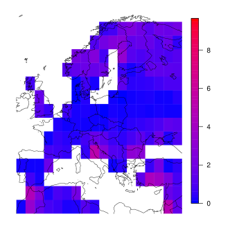
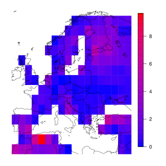
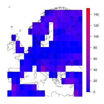
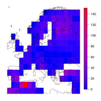
Our study region consists of large parts of Europe (8W–40E, 32N–74N) as illustrated in Figure 1. The climate model projections are obtained from the Coupled Model Intercomparison Project phase 3 (CMIP3) multi-model dataset [26]. The various models operate on distinct global grids. To allow for a grid based comparison, we transform to a common global grid of size , as used for the re-analysis data. At this resolution, our study region contains a total of 154 grid boxes. As observational data, we work with the ERA-40 re-analysis [27] by the European Centre for Medium-Range Weather Forecasts and the NCEP-1 re-analysis [28] by the U.S. National Centers for Environmental Prediction. In our comparison, we only use a single simulation from each of the 15 climate models; if multiple simulations are available, one instance is selected at random. Both the climate models and the re-analyses provide daily outputs for 2m maximum temperature. At each grid box, the climate model simulation then is represented by the location-specific empirical distribution function of the resulting annual maxima over the study period from 1961 to 1990.
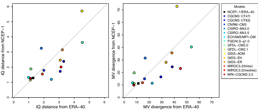
Figure 2 shows the integrated quadratic distance (6) in the unit of degrees Celsius and the mean value divergence (8) of the simulations from the two sets of re-analysis data, with each value being an average over the 154 grid boxes. The divergences result in similar rankings of the climate models relative to the re-analysis data sets. For three models, the divergences between the model and the re-analysis data are at the level of the internal variability between the ERA-40 and the NCEP-1 re-analyses, which is the best performance one might reasonably hope for. These are the ECHAM5/MPI-OM model from the Max Planck Institute for Meteorology in Germany, the GFDL-CM2.1 model developed by the Geophysical Fluid Dynamics Laboratory in the United States and the MRI-CGCM2.3.2 model from the Meteorological Research Institute of Japan. The first two models have a slightly higher spatial resolution than the re-analyses while the MRI-CGCM2.3.2 model operates on a grid of size .
In Figure 1, we can identify the location-specific divergences for the ECHAM5/MPI-OM model under both sets of re-analysis data. Any differences between the two re-analyses seem to be more pronounced in coastal regions, in particular around the Mediterranean Sea and on the Eastern shore of the Baltic Sea. As the two types of divergences operate on different scales, the results for the integrated quadratic distance cannot be compared directly to the mean value divergence. However, the results seem to indicate that there is more local variability under the integrated quadratic distance, as is to be expected, given that it addresses all distributional features, as opposed to the mean value divergence.
6 Discussion
We have introduced the notion of propriety for divergences, i.e., distance measures between probability distributions. In a nutshell, if the divergence is proper, and we believe that the observations form a sample from the probability distribution , then an optimal, expectation minimizing predictive distribution is . This property is important in settings such as that of Figure 2, where we compared climate models based on the average divergence between the probability distributions of model output and the corresponding empirical distributions of temperature extremes. Empirical means correspond to expectations and therefore, for a proper divergence function, the average divergence criterion favors skillful climate models in decision theoretically coherent ways. In this context, the question for meaningful or perhaps even optimal ways of averaging and aggregating deserves further study.
Score divergences tha t derive from proper scoring rules are -proper for all positive integers , with the integrated quadratic distance (6), the Dawid-Sebastiani divergence (9) and the Kullback-Leibler divergence (10) being particularly attractive choices, while other commonly used distances fail to be proper. In the case of real-valued variables, the integrated quadratic distance is the only divergence available that satisfies the desirable properties listed in the introduction, and thus we endorse and encourage its use.
The evaluation of model simulations continues to provide challenges. In this paper we have considered the case of individual climate model runs, which we have ranked based on their grid averaged divergences from re-analysis data sets. Fricker et al. [29] consider further simulation formats, such as ensemble hindcasts, and in the case of a single model run, their pooled ensemble CRPS [29, p. 252] equals the integrated quadratic distance. An important caveat is that if we evaluate model simulations for a univariate quantity, such as an annual temperature maximum, by using a divergence function, the assessment is restricted to univariate aspects. If multivariate aspects, such as the behavior of temperature extremes at several sites simultaneously, are of interest, divergence functions for probability distributions in higher-dimensional spaces are to be considered.
Acknowledgments
The work of Nadine Gissibl and Tilmann Gneiting has been supported by the European Union Seventh Framework Programme under grant agreement no. 290976, Thordis L. Thorarinsdottir acknowledges the support of sfi2, Statistics for Innovation in Oslo. We are grateful to Sebastian Mieruch, Jana Sillmann, Jon Wellner and Johanna Ziegel for discussions and/or assistance with the data handling, and thank an associate editor and two reviewers for constructive comments. We acknowledge the modeling groups, the Program for Climate Model Diagnosis and Intercomparison (PCMDI) and the World Climate Research Programme’s (WCRP’s) Working Group on Coupled Modelling (WGCM) for making the WCRP CMIP3 multi-model dataset available. Support of this dataset is provided by the Office of Science, U.S. Department of Energy.
References
- [1] P. J. Gleckler, K. E. Taylor and C. Doutriaux Performance metrics for climate models J. Geophys. Res. 113 (2008) D06104.
- [2] L. O. Mearns, R. Arritt, S. Biner, M. S. Bukovsky, S. McGinnis, S. Sain, D. Caya, J. Correia Jr, D. Flory, W. Gutowski, E. S. Takle,R. Jones, R. Leung, W. Moufouma-Okia, L. McDaniel, A. M. B. Nunes, Y. Qian, J. Roads, L. Sloan and M. Snyder The North American regional climate change assessment program: Overview of phase I results Bull. Am. Meteorol. Soc. 93 (2012) pp. 1337–1362.
- [3] P. Guttorp The role of statisticians in international science policy Environmetrics 22 (2011) pp. 817–825.
- [4] T. N. Palmer Towards the probabilistic Earth-system simulator: A vision for the future of climate and weather prediction Q. J. R. Meteorol. Soc. 138 (2012) pp. 841–861.
- [5] H. M. Arnold, I. M. Moroz and T. N. Palmer Stochastic parameterizations and model uncertainty in the Lorenz ’96 system Phil. Trans. R. Soc. A 371 (2013) 20110479.
- [6] S. E. Perkins, A. J. Pitman, N. J. Holbrook and J. McAneney Estimation of the AR4 climate models’ simulated daily maximum temperature, minimum temperature, and precipitation over Australia using probability density functions J. Clim. 20 (2007) pp. 4356–4376.
- [7] M. M. Deza and E. Deza Encyclopedia of Distances 2nd edition Springer Berlin 2013.
- [8] A. L. Gibbs and F. E. Su On choosing and bounding probability metrics Int. Stat. Rev. 70 (2002) pp. 419–435.
- [9] S. Ferson, W. L. Oberkampf and L. Ginzburg Model validation and predictive capability for the thermal challenge problem Computat. Meth. Appl. Mech. Eng. 197 (2008) pp. 2408–2430.
- [10] R. L. Winkler and A. H. Murphy “Good” probability assessors J. Appl. Meteorol. 7 (1968) pp. 751–758.
- [11] T. Gneiting and A. E. Raftery Strictly proper scoring rules, prediction, and estimation J. Am. Stat. Assoc. 102 (2007) pp. 359–378.
- [12] J. Bröcker and L. A. Smith Scoring probabilistic forecasts: The importance of being proper Wea. Forecasting 22 (2007) pp. 382–388.
- [13] Y. Liu, W. Chen, P. Arendt and H. Z. Huang Toward a better understanding of model validation metrics J. Mech. Design 133 (2011) 071005.
- [14] G. Székely and M. L. Rizzo Hierarchical clustering via joint between-within distances: Extending Ward’s minimum variance method J. Classific. 22 (2005) pp. 151–183.
- [15] J. E. Matheson and R. L. Winkler Scoring rules for continuous probability distributions Manag. Sci. 22 (1976) pp. 1087–1096.
- [16] E. Salazar, B. Sansó, A. O. Finley, D. Hammerling, I. Steinsland, X. Wang and P. Delamater Comparing and blending regional climate model predictions for the American Southwest J. Agric. Biol. Env. Stat. 16 (2011) pp. 586–605.
- [17] K. Hasselmann Optimal fingerprints for the detection of time-dependent climate change J. Clim. 6 (1993) pp. 1957–1971.
- [18] G. C. Hegerl, H. von Storch, K. Hasselmann, B. D. Santer, U. Cubasch and P. D. Jones Detecting greenhouse-gas-induced climate change with an optimal fingerprint method J. Clim. 9 (1996) pp. 2281–2306.
- [19] T. P. Barnett, D. W. Pierce, K. M. AchutaRao, P. J. Gleckler, B. D. Santer, J. M. Gregory and W. M. Washington Penetration of human-induced warming into the world’s oceans Science 309 (2005) pp. 284–287.
- [20] X. Zhang, F. W. Zwiers, G. C. Hegerl, F. H. Lambert, N. P. Gillett, S. Solomon, P. A. Stott and T. Nozawa Detection of human influence on twentieth-century precipitation trends Nature 448 (2007) pp. 461–465.
- [21] P. C. Mahalanobis On the generalized distance in statistics Proc. Natl. Inst. Sci. India 2 (1936) pp. 49–55.
- [22] A. P. Dawid and P. Sebastiani Coherent dispersion criteria for optimal experimental design Ann. Stat. 27 (1999) pp. 65–81.
- [23] G. R. Shorack and J. A. Wellner Empirical Processes with Applications to Statistics Wiley New York 1986.
- [24] P. Bickel and D. A. Freedman Some asymptotic theory for the bootstrap Ann. Stat. 9 (1981) pp. 1196–1217.
- [25] G. W. Brier Verification of forecasts expressed in terms of probability Mon. Wea. Rev. 78 (1950) pp. 1–3.
- [26] G. A. Meehl, C. Covey, T. Delworth, M. Latif, B. McAvaney, J. F. B. Mitchell, R. J. Stouffer and K. E. Taylor The WCRP CMIP3 multi-model dataset: A new era in climate change research Bull. Am. Meteorol. Soc. 88 (2007) pp. 1383–1394.
- [27] S. M. Uppala, P. W. Kållberg, A. J. Simmons, U. Andrae, V. D. C.Bechtold, M. Fiorino, J. K. Gibson, J. Haseler, A. Hernandez, G. A. Kelly, X. Li, K. Onogi, S. Saarinen, N. Sokka, R. P. Allan, E. Andersson, K. Arpe, M. A. Balmaseda, A. C. M. Beljaars, L. Van De Berg, J. Bidlot, N. Bormann, S. Caires, F. Chevallier, A. Dethof, M. Dragosavac, M. Fisher, M. Fuentes, S. Hagemann, E. Hólm, B. J. Hoskins, L. Isaksen, P. A. E. M. Janssen, R. Jenne, A. P. Mcnally, J.-F. Mahfouf, J.-J. Morcrette, N. A. Rayner, R. W. Saunders, P. Simon, A. Sterl, K. E. Trenberth, A. Untch, D. Vasiljevic, P. Viterbo and J. Woollen The ERA-40 re-analysis Q. J. R. Meteorol. Soc. 131 (2005) pp. 2961–3012.
- [28] E. Kalnay, M. Kanamitsu, R. Kistler, W. Collins, D. Deaven, L. Gandin, M. Iredell, S. Saha, G. White, J. Woollen, Y. Zhu, M. Chelliah, W. Ebisuzaki, W. Higgins, J. Janowiak, K. C. Mo, C. Ropelewski, J. Wang, A. Leetmaa, R. Reynolds, R. Jenne and D. Joseph The NCEP/NCAR 40-year reanalysis project Bull. Am. Meteorol. Soc. 77 (1996) pp. 437–470.
- [29] T. E. Fricker, C. A. T. Ferro and D. B. Stephenson Three recommendations for evaluating climate predictions Meteorol. Appl. 20 (2013) pp. 246–255.