Optimal Reconstruction of Material Properties in Complex Multiphysics Phenomena

Abstract

We develop an optimization–based approach to the problem of reconstructing
temperature–dependent material properties in complex thermo–fluid systems described by the equations for the conservation of mass, momentum and energy. Our goal is to estimate the temperature dependence of the viscosity coefficient in the momentum equation based on some noisy temperature measurements, where the temperature is governed by a separate energy equation. We show that an elegant and computationally efficient solution of this inverse problem is obtained by formulating it as a PDE–constrained optimization problem which can be solved with a gradient–based descent method. A key element of the proposed approach, the cost functional gradients are characterized by mathematical structure quite different than in typical problems of PDE–constrained optimization and are expressed in terms of integrals defined over the level sets of the temperature field. Advanced techniques of integration on manifolds are required to evaluate numerically such gradients, and we systematically compare three different methods. As a model system we consider a two–dimensional unsteady flow in a lid–driven cavity with heat transfer, and present a number of computational tests to validate our approach and illustrate its performance.

Keywords: parameter estimation, material properties, optimization, adjoint analysis, integration on level sets.

1 Introduction

In this work we propose and validate a computational approach to the reconstruction of material properties in complex multiphysics phenomena based on incomplete and possibly noisy measurements. The material properties we are interested in here are the transport coefficients characterizing diffusion processes such as the viscosity or the thermal conductivity, and we focus on problems in which these coefficients depend on the state variables in the system. By the “multiphysics” aspect we mean situations in which the material property used in one conservation equation is a function of a state variable governed by a different conservation equation, e.g., reconstruction of the temperature dependence of the viscosity coefficient used in the momentum equation, where the temperature is governed by a separate energy equation, which is the specific model problem investigated in this study. This research is motivated by questions arising in the computational analysis and optimization of advanced welding processes which involves modelling complex alloys in the liquid phase at high temperatures [1].

Inverse problems of parameter estimation for partial differential equations (PDEs) have received significant attention in the literature, both regarding theoretical [2] and practical aspects [3]. However, most of the attention focused on problems in which the material properties are functions of the space variable (i.e., the independent variable in the problem). Such problems are, at least in principle, relatively well understood and represent the foundation of, for example, numerous imaging techniques in medicine [4] and earth sciences [5]. The problem considered here is in fact different, in that the material properties are sought as functions of the state (dependent) variables in the system which gives rise to a number of computational challenges absent in the “classical” parameter estimation problem. Other than the seminal work of Chavent and Lemonnier [6], our earlier study [7] concerning a simplified model problem and a few investigations of fully discrete formulations surveyed in [7], there does not seem to be much literature concerning computational methods for this type of parameter estimation problems. One way to solve such inverse problems is to formulate them as optimization problems and this is the approach we will follow focusing on the “optimize–then–discretize” paradigm in which the optimality conditions are formulated at the continuous (PDE) level and only then discretized. The goal of this investigation is to extend the approach formulated in [7] for a simple model to a realistic multiphysics problem involving time–dependent fluid flow in a two–dimensional (2D) domain. As will be shown below, a number of computational difficulties will need to be overcome in order to achieve this goal.

As a key contribution of this work, we address a number of computational challenges related to accurate and efficient evaluation of cost functional gradients which are critical to the implementation of the proposed approach. More specifically, these gradients are given in terms of integrals of expressions involving state and adjoint variables defined on a grid over contours given by the level sets of the temperature field. A number of techniques have been proposed for the numerical evaluation of integrals defined over manifolds defined by level–set functions. Some of them rely on regularized Dirac delta and Heaviside functions [9, 8], or discretization of the Dirac delta function [11, 10, 12]. Similar approaches, based on approximations of the Dirac delta functions obtained using the level–set function and its gradient, were developed by Towers [13, 14]. The family of geometric approaches proposed by Min and Gibou in [15, 16] relies on a decomposition of the entire domain into simplices. We emphasize that the problem discussed in this work is in fact more complicated, as the computation of our cost functional gradients requires evaluation of the corresponding integrals for the level–set values spanning the entire state space of interest, hence there are also additional issues related to the discretization of the state space which were outside the scope of references [8, 9, 10, 11, 12, 15, 16, 13, 14]. Thus, in order to address these questions and assess the different trade–offs in the choice of the numerical parameters we will compare the computational performance of three different methods for the evaluation of cost functional gradients.

The structure of this paper is as follows: in the next Section we formulate our model problem, in the following Section we cast the problem of parameter estimation as an optimization problem, an adjoint–based gradient–descent algorithm is formulated in Section 4, in Section 5 we outline some regularization strategies needed in the presence of measurement noise, whereas in Section 6 we analyze three different numerical approaches to the evaluation of the cost functional gradients; extensive computational results are presented in Section 7 with discussion and conclusions deferred to Section 8.

2 Model Problem

Let $\Omega\subset{\mathbb{R}}^{d}$, $d=2,3$, be the spatial domain on which our model problem is formulated. To fix attention, but without loss of generality, in the present investigation we focus on the problem of a reconstruction of the temperature dependence $\mu=\mu(T)$ of the viscosity coefficient $\mu\>:\>{\mathbb{R}}\rightarrow{\mathbb{R}}^{+}$ in the momentum equation (Navier-Stokes equation), where the temperature $T$ is governed by a separate energy equation

$$\partial_{t}{\bf u}+({\bf u}\cdot\boldsymbol{\nabla}){\bf u}+\boldsymbol{\nabla}p-\boldsymbol{\nabla}\cdot\left[\mu(T)[\boldsymbol{\nabla}{\bf u}+(\boldsymbol{\nabla}{\bf u})^{T}]\right] = 0\qquad \textrm{in}\ \Omega,$$ (1a)

$$\boldsymbol{\nabla}\cdot{\bf u} = 0\qquad \textrm{in}\ \Omega,$$ (1b)

$$\partial_{t}T+({\bf u}\cdot\boldsymbol{\nabla})T-\boldsymbol{\nabla}\cdot[k\boldsymbol{\nabla}T] = 0\qquad \textrm{in}\ \Omega,$$ (1c)

subject to appropriate Dirichlet (or Neumann) boundary and initial conditions

$${\bf u} ={\bf u}_{B}\qquad \textrm{on}\ \partial\Omega,$$ (2a)

$$T =T_{B}\qquad \textrm{on}\ \partial\Omega,$$ (2b)

$${\bf u}(\cdot,0) ={\bf u}_{0},\ T(\cdot,0)=T_{0}\qquad \textrm{in}\ \Omega.$$ (2c)

The specific inverse problem we address in this investigation is formulated as follows. Given a set of time–dependent “measurements” $\{\tilde{T}_{i}(t)\}_{i=1}^{M}$ of the state variable (temperature) $T$ at a number of points $\{{\bf x}_{i}\}_{i=1}^{M}$ in the domain $\Omega$ (or along the boundary $\partial\Omega$) and obtained within the time window $t\in[0,t_{f}]$, we seek to reconstruct the constitutive relation $\mu=\mu(T)$ such that solutions of problem (1)-(2) obtained with this reconstructed function will fit best the available measurements.

In regard to reconstruction of constitutive relations in general, it is important that such relations be consistent with the second principle of thermodynamics [17]. There exist two mathematical formalisms, one due to Coleman and Noll [18] and another one due to Liu [19], developed to ensure in a very general setting that a given form of the constitutive relation does not violate the second principle of thermodynamics. In continuous thermodynamical and mechanical systems this principle is expressed in terms of the Clausius–Duhem inequality [20] which in the case of our present model problem (1)–(2) reduces to the statement that $\mu(T)>0$ for all possible values of $T$.

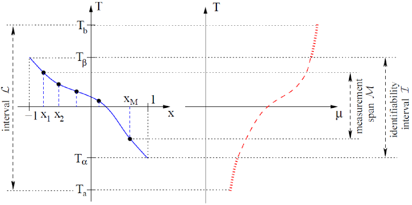
In our discussion below we will also need definitions of the following intervals, cf. Figure 1:

• $[T_{\alpha},T_{\beta}]\triangleq[\min_{{\bf x}\in\overline{\Omega}}T({\bf x}),\max_{{\bf x}\in\overline{\Omega}}T({\bf x})]$ which represents the temperature range spanned by the solution of problem (1); thus, following [21], we will refer to the interval ${\mathcal{I}}\triangleq[T_{\alpha},T_{\beta}]$ as the identifiability interval,

• ${\mathcal{L}}\triangleq[T_{a},T_{b}]$, where $T_{a}\leq T_{\alpha}$ and $T_{b}\geq T_{\beta}$; this will be the temperature interval on which we will seek to obtain a reconstruction of the material property; we note that in general the interval ${\mathcal{L}}$ will be larger than the identifiability interval, i.e., ${\mathcal{I}}\subseteq{\mathcal{L}}$, and

• ${\mathcal{M}}\triangleq[\min_{1\leq i\leq M}\min_{0<t\leq t_{f}}\tilde{T}_{i}(t),\max_{1\leq i\leq M}\max_{0<t\leq t_{f}}\tilde{T}_{i}(t)]$ which defines the temperature range spanned by the measurements $\{\tilde{T}_{i}\}_{i=1}^{M}$; this interval is always contained the identifiability interval ${\mathcal{I}}$, i.e., ${\mathcal{M}}\subseteq{\mathcal{I}}$; we will refer to the interval ${\mathcal{M}}$ as the measurement span.

Figure 1: Schematic showing (left) the solution $T(t_{0},x)$ at some fixed time $t_{0}$ and (right) the corresponding constitutive relation $\mu(T)$ defined over their respective domains, i.e., $\Omega=(-1,1)$ and the identifiability region ${\mathcal{I}}$. The thick dotted line represents an extension of the constitutive relation $\mu(T)$ from ${\mathcal{I}}$ to the interval ${\mathcal{L}}$. In the Figure on the right the horizontal axis is to be interpreted as the ordinate.

3 Parameter Estimation as an Optimization Problem

It is assumed that the constitutive relations $\mu(T)$ are differentiable functions of the state variable (temperature) and belong to the following set

$${\mathcal{S}}_{\mu}=\{\mu(T)\ \textrm{piecewise}\ C^{1}\ \textrm{on}\ {\mathcal{L}};\ 0<m_{\mu}\leq\mu(T)\leq M_{\mu}<\infty,\ \forall\,T\in{\mathcal{L}}\},$$ (3)

where $m_{\mu},M_{\mu}\in{\mathbb{R}}^{+}$. We will also assume that the set ${\mathcal{S}}_{\mu}$ consisting of constitutive relations $\mu(T)$ defined on ${\mathcal{L}}$ is embedded in a Hilbert (function) space ${\mathcal{X}}$ to be specified below. Solving our parameter estimation problem is therefore equivalent to finding a solution to the operator equation

$${\mathcal{F}}(\mu)=T,$$ (4)

where ${\mathcal{F}}\,:\,{\mathcal{S}}_{\mu}\rightarrow\left(L_{2}([0,t_{f}])\right)^{M}$ is the map from the constitutive relations to the measurements. An approach commonly used to solve such problems consists in reformulating them as least–squares minimization problems which in the present case can be done by defining the cost functional ${\mathcal{J}}\>:\>{\mathcal{X}}\rightarrow{\mathbb{R}}$ as

$${\mathcal{J}}(\mu)\triangleq\frac{1}{2}\int_{0}^{t_{f}}\sum_{i=1}^{M}\left[T(\tau,{\bf x}_{i};\mu)-\tilde{T}_{i}(\tau)\right]^{2}d\tau,$$ (5)

where the dependence of the temperature field $T(\cdot;\mu)$ on the form of the constitutive relation $\mu=\mu(T)$ is given by governing system (1)–(2). The optimal reconstruction $\hat{\mu}$ is obtained as a minimizer of cost functional (5), i.e.,

$$\hat{\mu}=\underset{\mu\in{\mathcal{S}}_{\mu}}{\operatorname{argmin}}\,{\mathcal{J}}(\mu).$$ (6)

We recall that the constitutive property is required to satisfy the positivity condition $\mu(T)>0$ for all $T\in{\mathcal{L}}$, cf. (3). Therefore, the optimal reconstruction $\hat{\mu}$ should in fact be obtained as an inequality–constrained minimizer of cost functional (5), i.e.,

$$\hat{\mu}=\underset{\stackrel{{\scriptstyle\mu\in{\mathcal{X}},}}{{\mu(T)>0,\ T\in{\mathcal{L}}}}}{\operatorname{argmin}}{\mathcal{J}}(\mu).$$ (7)

We add that in problems involving constitutive relations depending on several state variables the inequality constraint $\mu(T)>0$ will be replaced with a more general form of the Clausius–Duhem inequality [20]. Different computational approaches for converting inequality–constrained optimization problems to unconstrained formulations are surveyed in [22, 23]. Here we follow a straightforward approach based on the so-called “slack” variable [24]. We define a new function $\theta(T)\>:\>{\mathbb{R}}\rightarrow{\mathbb{R}}$ such that

$$\mu(T)=\theta^{2}(T)+m_{\mu},$$ (8)

where $m_{\mu}$ is a lower bound for $\mu(T)$, cf. (3). This change of variables allows us to transform the inequality–constrained optimization problem (7) to a new unconstrained one

$$\hat{\theta}=\underset{\theta\in{\mathcal{X}}}{\operatorname{argmin}}\,{\mathcal{J}}(\theta),$$ (9)

where the constraint $\mu(T)>0$ is satisfied automatically when minimization is performed with respect to the new variable $\theta(T)$. In view of (3), we note that the new optimization variable $\theta$ belongs to the following set

$${\mathcal{S}}_{\theta}=\{\theta(T)\ \textrm{piecewise}\ C^{1}\ \textrm{on}\ {\mathcal{L}};\ |\theta(T)|<\sqrt{M_{\mu}-m_{\mu}},\ \forall\,T\in{\mathcal{L}}\}.$$ (10)

The governing PDE system (1) can thus be rewritten in the form

$$\partial_{t}{\bf u}+({\bf u}\cdot\boldsymbol{\nabla}){\bf u}+\boldsymbol{\nabla}p-\boldsymbol{\nabla}\cdot\left[(\theta^{2}(T)+m_{\mu})[\boldsymbol{\nabla}{\bf u}+(\boldsymbol{\nabla}{\bf u})^{T}]\right] = 0\qquad \textrm{in}\ \Omega,$$ (11a)

$$\boldsymbol{\nabla}\cdot{\bf u} = 0\qquad \textrm{in}\ \Omega,$$ (11b)

$$\partial_{t}T+({\bf u}\cdot\boldsymbol{\nabla})T-\boldsymbol{\nabla}\cdot[k\boldsymbol{\nabla}T] = 0\qquad \textrm{in}\ \Omega,$$ (11c)

subject to Dirichlet boundary and initial conditions (2). The new problem (9) requires redefining cost functional (5) in terms of the new variable

$${\mathcal{J}}(\theta)=\frac{1}{2}\int_{0}^{t_{f}}\sum_{i=1}^{M}\left[T(\tau,{\bf x}_{i};\theta)-\tilde{T}_{i}(\tau)\right]^{2}\,d\tau.$$ (12)

Problem (9) is characterized by the first–order optimality condition which requires the Gâteaux differential of cost functional (12), defined as ${\mathcal{J}}^{\prime}(\theta;\theta^{\prime})\triangleq\lim_{\epsilon\rightarrow 0}\epsilon^{-1}[{\mathcal{J}}(\theta+\epsilon\theta^{\prime})-{\mathcal{J}}(\theta)]$, to vanish for all perturbations $\theta^{\prime}\in{\mathcal{X}}$ [25], i.e.,

$$\forall_{\theta^{\prime}\in{\mathcal{X}}}\ \ {\mathcal{J}}^{\prime}(\hat{\theta};\theta^{\prime})=0.$$ (13)

The (local) optimizer $\hat{\theta}$ can be computed with the following gradient descent algorithm as $\hat{\theta}=\lim_{n\rightarrow\infty}\theta^{(n)}$, where

$$\left\{\begin{aligned} &\theta^{(n+1)}&&=\theta^{(n)}-\tau^{(n)}\boldsymbol{\nabla}_{\theta}{\mathcal{J}}(\theta^{(n)}),\qquad n=1,\dots,\\ &\theta^{(1)}&&=\theta_{0},\end{aligned}\right.$$ (14)

in which $\boldsymbol{\nabla}_{\theta}{\mathcal{J}}(\theta)$ represents the gradient of cost functional ${\mathcal{J}}(\theta)$ with respect to the control variable $\theta$ (we will adopt the convention that a subscript on the operator $\boldsymbol{\nabla}$ will be used when differentiation is performed with respect to variables other than ${\bf x}$), $\tau^{(n)}$ is the length of the step along the descent direction at the $n$–th iteration, whereas $\theta_{0}=\sqrt{\mu_{0}-m_{\mu}}$ is the initial guess taken, for instance, corresponding to a constant $\mu_{0}$, or some other appropriate initial approximation. For the sake of clarity, formulation (14) represents the steepest–descent algorithm, however, in practice one typically uses more advanced minimization techniques, such as the conjugate gradient method, or one of the quasi–Newton techniques [26]. We note that, since minimization problem (9) is in general nonconvex, condition (13) characterizes only a local, rather than global, minimizer.

The key ingredient of minimization algorithm (14) is computation of the cost functional gradient $\boldsymbol{\nabla}_{\theta}{\mathcal{J}}(\theta)$. We emphasize that, since $\theta=\theta(T)$ is a continuous variable, the gradient $\boldsymbol{\nabla}_{\theta}{\mathcal{J}}(\theta)$ represents in fact the infinite–dimensional sensitivity of ${\mathcal{J}}(\theta)$ to perturbations of $\theta(T)$. This gradient can be determined based on suitably defined adjoint variables (Lagrange multipliers) obtained from the solution of the corresponding adjoint system. Since this derivation differs in a number of imported technical details from analogous derivations in “standard” PDE–constrained optimization problems, it will be reviewed in Section 4. The expression for the gradient is then validated for consistency in Section 7.4.

4 Cost Functional Gradients via Adjoint–based Analysis

Since the new variable $\theta(T)$ belongs to set ${\mathcal{S}}_{\theta}$, cf. (10), we will seek to reconstruct $\theta(T)$ as elements of the Sobolev space $H^{1}({\mathcal{L}})$, so that the gradient $\boldsymbol{\nabla}_{\theta}{\mathcal{J}}$ will need to be obtained with respect to the corresponding inner product. However, in order to make the derivation procedure easier to follow, we will first obtain an expression for the gradient in the space $L_{2}({\mathcal{L}})$, and only then will obtain the Sobolev gradients which will be eventually used in the solution of optimization problem (9). In all these steps our transformations will be formal. We begin by computing the directional (Gâteaux) differential of cost functional (12) which yields

$${\mathcal{J}}^{\prime}(\theta;\theta^{\prime})=\int_{0}^{t_{f}}\sum_{i=1}^{M}[T(\tau,{\bf x}_{i};\theta)-\tilde{T}_{i}(\tau)]\,T^{\prime}(\tau,{\bf x}_{i};\theta,\theta^{\prime})\,d\tau,$$ (15)

where the perturbation variable $T^{\prime}(\theta,\theta^{\prime})$ satisfies the perturbation system obtained from (1)–(2). Next, we invoke the Riesz representation theorem [27] for the directional differential ${\mathcal{J}}^{\prime}(\theta;\cdot)$ which yields

$${\mathcal{J}}^{\prime}(\theta;\theta^{\prime})=\Big{\langle}\boldsymbol{\nabla}_{\theta}{\mathcal{J}},\theta^{\prime}\Big{\rangle}_{{\mathcal{X}}},$$ (16)

where $\langle\cdot,\cdot\rangle_{{\mathcal{X}}}$ represents an inner product in the Hilbert space ${\mathcal{X}}$ (we will first set ${\mathcal{X}}=L_{2}({\mathcal{L}})$ and afterwards change this to ${\mathcal{X}}=H^{1}({\mathcal{L}})$). We note that the expression on the right–hand side (RHS) in (15) is not consistent with Riesz representation (16), since, as will be shown below, the perturbation variable $\theta^{\prime}$ is hidden in the system defining $T^{\prime}(\theta,\theta^{\prime})$. However, this expression can be transformed to Riesz form (16) with the help of a suitably–defined adjoint variable, a result which is stated in Theorem 19 below. The main aspect in which this derivation differs from the standard adjoint analysis [28] is that the inner product in Riesz identity (16) is defined using the state variable (temperature) as the integration variable, whereas the variational formulation of (1)–(2) is defined using integration with respect to the independent variables (${\bf x}$ and $t$).

Theorem 4.1.

Let $\Omega$ be a sufficiently regular open bounded domain and $\theta^{\prime}\in{\mathcal{X}}=H^{1}({\mathcal{L}})$. We assume that the solutions ${\bf u}$ and $T$ of system (1)–(2) are sufficiently smooth. Then, the Riesz representation of directional differential (15) has the form

$${\mathcal{J}}^{\prime}(\theta;\theta^{\prime})=-2\int_{-\infty}^{\infty}\int_{\Omega}\delta(T({\bf x})-s)\,\theta(s)\,\left[\int^{t_{f}}_{0}[\boldsymbol{\nabla}{\bf u}+(\boldsymbol{\nabla}{\bf u})^{T}]:\boldsymbol{\nabla}{\bf u}^{*}\,d\tau\right]\,\theta^{\prime}(s)\,d{\bf x}\,ds,$$ (17)

where $\delta(\cdot)$ denotes Dirac delta function and the adjoint state $\{{\bf u}^{*},T^{*}\}$ is defined as the solution of the system

$$-\partial_{t}{\bf u}^{*}-({\bf u}\cdot\boldsymbol{\nabla}){\bf u}^{*}-\boldsymbol{\nabla}\cdot\boldsymbol{\sigma}^{*}+{\bf u}^{*}\cdot(\boldsymbol{\nabla}{\bf u})^{T}+T^{*}\boldsymbol{\nabla}T =0\qquad \mathrm{in}\ \Omega,$$ (18a)

$$\boldsymbol{\nabla}\cdot{\bf u}^{*} =0\qquad \mathrm{in}\ \Omega,$$ (18b)

$$-\partial_{t}T^{*}-({\bf u}\cdot\boldsymbol{\nabla})T^{*}-\boldsymbol{\nabla}\cdot[k\boldsymbol{\nabla}T^{*}]+2\theta(T)\,\dfrac{d\theta}{dT}(T)\,[\boldsymbol{\nabla}{\bf u}+(\boldsymbol{\nabla}{\bf u})^{T}]:\boldsymbol{\nabla}^{*}{\bf u}$$

$$=\sum_{i=1}^{M}[T({\bf x}_{i};\theta)-\tilde{T}_{i}]\delta({\bf x}-{\bf x}_{i}) \mathrm{in}\ \Omega,$$ (18c)

where $\boldsymbol{\sigma}^{*}\triangleq-p^{*}{\mathcal{I}}+(\theta^{2}(T)+m_{\mu})\left[\boldsymbol{\nabla}{\bf u}^{*}+(\boldsymbol{\nabla}{\bf u}^{*})^{T}\right]$, with the following boundary and terminal conditions

$${\bf u}^{*} =0\qquad \mathrm{on}\ \partial\Omega,$$ (19)

$$T^{*} =0\qquad \mathrm{on}\ \partial\Omega,$$

$${\bf u}^{*}(\cdot;t_{f}) =0,\ T^{*}(\cdot;t_{f})=0\qquad \mathrm{in}\ \Omega.$$

Proof.

We will denote the stress tensor $\boldsymbol{\sigma}\triangleq-p{\mathcal{I}}+(\theta^{2}(T)+m_{\mu})\left[\boldsymbol{\nabla}{\bf u}+(\boldsymbol{\nabla}{\bf u})^{T}]\right]$ and rewrite the governing system (11) as

$$\partial_{t}{\bf u}+({\bf u}\cdot\boldsymbol{\nabla}){\bf u}-\boldsymbol{\nabla}\cdot\boldsymbol{\sigma} = 0 \textrm{in}\ \Omega,$$ (20)

$$\boldsymbol{\nabla}\cdot{\bf u} = 0 \textrm{in}\ \Omega,$$

$$\partial_{t}T+({\bf u}\cdot\boldsymbol{\nabla})T-\boldsymbol{\nabla}\cdot[k\boldsymbol{\nabla}T] = 0 \textrm{in}\ \Omega$$

with the boundary and initial conditions (2). Perturbing the state variables ${\bf u}$, $p$ and $T$, which are functions of time and space, we get

$${\bf u} ={\bf u}_{0}+\epsilon{\bf u}^{\prime}+{\mathcal{O}}(\epsilon^{2}),$$ (21)

$$p =p_{0}+\epsilon p^{\prime}+{\mathcal{O}}(\epsilon^{2}),$$

$$T =T_{0}+\epsilon T^{\prime}+{\mathcal{O}}(\epsilon^{2}),$$

so that the corresponding expansion of the constitutive relation $\theta(T)$ will have the following form

$$\theta(T)=\theta_{0}(T)+\epsilon\theta^{\prime}(T)+{\mathcal{O}}(\epsilon^{2})=\theta_{0}(T_{0})+\epsilon\dfrac{d\theta}{dT}(T_{0})\,T^{\prime}(\theta_{0};\theta^{\prime})+\epsilon\theta^{\prime}(T_{0})+{\mathcal{O}}(\epsilon^{2}),$$ (22)

where the subscript “$0$” is used to denote the unperturbed (reference) material property and the state variable, whereas the prime denotes the corresponding perturbations. We also have

$$\theta^{2}(T)=\theta^{2}_{0}(T_{0})+2\epsilon\theta_{0}(T_{0})\,\dfrac{d\theta}{dT}(T_{0})\,T^{\prime}(\theta_{0};\theta^{\prime})+2\epsilon\theta_{0}(T_{0})\theta^{\prime}(T_{0})+{\mathcal{O}}(\epsilon^{2}).$$ (23)

Substituting (21) and (23) into (20), collecting terms corresponding to $\epsilon$ in different powers and denoting

$${}\hat{\boldsymbol{\sigma}} \triangleq-p^{\prime}{\mathcal{I}}+(\theta^{2}(T)+m_{\mu})\left[\boldsymbol{\nabla}{\bf u}^{\prime}+(\boldsymbol{\nabla}{\bf u}^{\prime})^{T}\right],$$

$$\tilde{\boldsymbol{\sigma}} \triangleq\left(2\theta(T)\,\dfrac{d\theta}{dT}(T)\,T^{\prime}(\theta_{0};\theta^{\prime})+2\theta(T)\,\theta^{\prime}(T)\right)\left[\boldsymbol{\nabla}{\bf u}+(\boldsymbol{\nabla}{\bf u})^{T}\right],$$

we obtain the perturbation (sensitivity) system corresponding to (11)

$$\partial_{t}{\bf u}^{\prime}+({\bf u}^{\prime}\cdot\boldsymbol{\nabla}){\bf u}+({\bf u}\cdot\boldsymbol{\nabla}){\bf u}^{\prime}-\boldsymbol{\nabla}\cdot(\hat{\boldsymbol{\sigma}}+\tilde{\boldsymbol{\sigma}}) = 0\qquad \textrm{in}\ \Omega,$$ (24a)

$$\boldsymbol{\nabla}\cdot{\bf u}^{\prime} = 0\qquad \textrm{in}\ \Omega,$$ (24b)

$$\partial_{t}T^{\prime}+({\bf u}^{\prime}\cdot\boldsymbol{\nabla})T+({\bf u}\cdot\boldsymbol{\nabla})T^{\prime}-\boldsymbol{\nabla}\cdot[k\boldsymbol{\nabla}T^{\prime}] = 0\qquad \textrm{in}\ \Omega$$ (24c)

with the following boundary and initial conditions

$${\bf u}^{\prime} =0\qquad \textrm{on}\ \partial\Omega,$$ (25a)

$$T^{\prime} =0\qquad \textrm{on}\ \partial\Omega,$$ (25b)

$${\bf u}^{\prime}(\cdot,0) =0,\ T^{\prime}(\cdot,0)=0\qquad \textrm{in}\ \Omega.$$ (25c)

Then, integrating equation (24a) against ${\bf u}^{*}$, equation (24b) against $p^{*}$, and equation (24c) against $T^{*}$ over the space domain $\Omega$ and time $[0,t_{f}]$, integrating by parts and factorizing ${\bf u}^{\prime}$, $T^{\prime}$ and $p^{\prime}$, we arrive at the following relation

$$\int^{t_{f}}_{0}\int_{\Omega}\left[-\partial_{t}{\bf u}^{*}+{\bf u}^{*}\cdot(\boldsymbol{\nabla}{\bf u})^{T}-({\bf u}\cdot\boldsymbol{\nabla}){\bf u}^{*}-\boldsymbol{\nabla}\cdot\boldsymbol{\sigma}^{*}+T^{*}\boldsymbol{\nabla}T\right]\cdot{\bf u}^{\prime}\,d{\bf x}\,d\tau$$ (26)

$$- \int^{t_{f}}_{0}\int_{\Omega}(\boldsymbol{\nabla}\cdot{\bf u}^{*})p^{\prime}\,d{\bf x}\,d\tau$$

$$+ \int^{t_{f}}_{0}\int_{\Omega}\left[-\partial_{t}T^{*}-({\bf u}\cdot\boldsymbol{\nabla})T^{*}-\boldsymbol{\nabla}\cdot(k\boldsymbol{\nabla}T^{*})+2\theta(T)\dfrac{d\theta}{dT}(T)[\boldsymbol{\nabla}{\bf u}+(\boldsymbol{\nabla}{\bf u})^{T}]:\boldsymbol{\nabla}{\bf u}^{*}\right]T^{\prime}\,d{\bf x}\,d\tau$$

$$+ \int^{t_{f}}_{0}\int_{\Omega}2\theta(T)\theta^{\prime}(T)[\boldsymbol{\nabla}{\bf u}+(\boldsymbol{\nabla}{\bf u})^{T}]:\boldsymbol{\nabla}{\bf u}^{*}\,d{\bf x}\,d\tau=0.$$

We now require that the adjoint variables ${\bf u}^{*}$, $p^{*}$ and $T^{*}$ satisfy system (18)–(19). We also note that owing to the judicious choice of the RHS term in (18c), the last term in relation (26) is in fact equal to the directional differential ${\mathcal{J}}^{\prime}(\theta;\theta^{\prime})$, so that we have

$${\mathcal{J}}^{\prime}(\theta;\theta^{\prime})=-2\int^{t_{f}}_{0}\int_{\Omega}\theta(T({\bf x},\tau))\theta^{\prime}(T({\bf x},\tau))\,[\boldsymbol{\nabla}{\bf u}({\bf x},\tau)+(\boldsymbol{\nabla}{\bf u}({\bf x},\tau))^{T}]:\boldsymbol{\nabla}{\bf u}^{*}({\bf x},\tau)\,d{\bf x}\,d\tau,$$ (27)

where, for emphasis, we indicated the integration variables as arguments of the state and adjoint variables. We note that this expression is still not in Riesz form (16), where integration must be performed with respect to the state variable (temperature $T$). Thus, we proceed to express for any given function $f(T)$ its pointwise evaluation at $T({\bf x})$ through the following integral transform. It is defined using a “change–of–variable” operator, denoted $\Pi$, such that for given functions $f\,:\,{\mathbb{R}}\rightarrow{\mathbb{R}}$ and $T\,:\,\Omega\rightarrow{\mathbb{R}}$, we have

$$f(T({\bf x}))=\int_{-\infty}^{+\infty}\delta(T({\bf x})-s)f(s)\,ds\triangleq(\Pi f)({\bf x}).$$ (28)

Using this transform to express $f(T({\bf x}))=\theta(T({\bf x},\tau))\theta^{\prime}(T({\bf x},\tau))$ in (27) and changing the order of integration (Fubini’s Theorem), we obtain expression (17) which is the required Riesz representation (16) of directional differential (15). ∎

We remark that we were able to prove an analogous result using a simpler approach based on the Kirchhoff transform in [7], where both the constitutive relation and the state variable were governed by the same equation (i.e., the problem was not of the “multiphysics” type).

With the Riesz representation established in (17), we now proceed to identify expressions for the cost functional gradient $\boldsymbol{\nabla}_{\theta}{\mathcal{J}}$ according to (16) using different spaces ${\mathcal{X}}$. While this is not the gradient that we will use in actual computations, we analyze first the “simplest” case when ${\mathcal{X}}=L_{2}({\mathcal{L}})$, i.e., the space of functions square integrable on $[T_{a},T_{b}]$, as it already offers some interesting insights into the structure of the problem. The $L_{2}$ gradient of the cost functional hence takes the form

$$\boldsymbol{\nabla}_{\theta}^{L_{2}}{\mathcal{J}}(s)=-2\int_{0}^{t_{f}}\int_{\Omega}\delta(T({\bf x})-s)\,\theta(s)\,[\boldsymbol{\nabla}{\bf u}+(\boldsymbol{\nabla}{\bf u})^{T}]:\boldsymbol{\nabla}{\bf u}^{*}\ d{\bf x}\,d\tau.$$ (29)

As was discussed at length in [7], the $L_{2}$ gradients are not suitable for the reconstruction of material properties in the present problem, because in addition to lacking necessary smoothness, they are not defined outside the identifiability region (other than perhaps through a trivial extension with zero). Given the regularity required of the constitutive relations, cf. (10), the cost functional gradients should be elements of the Sobolev space $H^{1}({\mathcal{L}})$ of functions with square–integrable derivatives on ${\mathcal{L}}$. Using (16), now with ${\mathcal{X}}=H^{1}({\mathcal{L}})$, we obtain

$${\mathcal{J}}^{\prime}(\theta;\theta^{\prime}) =\Big{\langle}\boldsymbol{\nabla}_{\theta}^{L_{2}}{\mathcal{J}},\theta^{\prime}\Big{\rangle}_{L_{2}({\mathcal{L}})}=\Big{\langle}\boldsymbol{\nabla}_{\theta}^{H^{1}}{\mathcal{J}},\theta^{\prime}\Big{\rangle}_{H^{1}({\mathcal{L}})}$$ (30)

$$=\int_{T_{a}}^{T_{b}}\left[(\boldsymbol{\nabla}_{\theta}^{H^{1}}{\mathcal{J}})\,\theta^{\prime}+\ell^{2}\frac{d(\boldsymbol{\nabla}_{\theta}^{H^{1}}{\mathcal{J}})}{ds}\frac{d\theta^{\prime}}{ds}\right]\,ds$$

in which $\ell\in{\mathbb{R}}$ is a parameter with the meaning of a “temperature–scale” [we note that the $L_{2}$ inner product is recovered by setting $\ell=0$ in (30)]. Performing integration by parts with the assumption that the Sobolev gradient $\boldsymbol{\nabla}_{\theta}^{H^{1}}{\mathcal{J}}$ satisfies the homogeneous Neumann boundary conditions at $T=T_{a},T_{b}$, and noting that relation (30) must be satisfied for any arbitrary $\theta^{\prime}$, we conclude that the Sobolev gradient can be determined as a solution of the following inhomogeneous elliptic boundary–value problem where the state variable (temperature) acts as the independent variable

$$\boldsymbol{\nabla}_{\theta}^{H^{1}}{\mathcal{J}}-\ell^{2}\frac{d^{2}}{ds^{2}}\boldsymbol{\nabla}_{\theta}^{H^{1}}{\mathcal{J}} =\boldsymbol{\nabla}_{\theta}^{L_{2}}{\mathcal{J}}\qquad \textrm{on}\ (T_{a},T_{b}),$$ (31a)

$$\frac{d}{ds}\boldsymbol{\nabla}_{\theta}^{H^{1}}{\mathcal{J}} =0 \textrm{for}\ s=T_{a},T_{b}.$$ (31b)

We recall that by changing the value of the temperature–scale parameter $\ell$ we can control the smoothness of the gradient $\boldsymbol{\nabla}_{\theta}^{H^{1}}{\mathcal{J}}(\theta)$, and therefore also the relative smoothness of the resulting reconstruction of $\theta(T)$, and hence also the regularity of $\mu(T)$. More specifically, as was shown in [29], extracting cost functional gradients in the Sobolev spaces $H^{p}$, $p>0$, is equivalent to applying a low–pass filter to the $L_{2}$ gradient with the quantity $\ell$ representing the “cut-off” scale. There are also other ways of defining the Sobolev gradients in the present problem which result in gradients characterized by a different behavior outside the identifiability region. These approaches were thoroughly investigated in [7], and since they typically lead to inferior results, they will not be considered here. We finally conclude that iterative reconstruction of the constitutive relation $\mu(T)$ involves the following computations

1. solution of direct problem (11) with boundary and initial conditions (2),

2. solution of adjoint problem (18)–(19),

3. evaluation of expression (29) for the cost functional gradient,

4. computation of the smoothed Sobolev gradient by solving (31).

While steps (1), (2) and (4) are fairly straightforward, step (3) is not and will be thoroughly investigated in Section 6.

As we discussed in detail in [7], while the Sobolev gradient $\boldsymbol{\nabla}_{\theta}^{H^{1}}{\mathcal{J}}$ may be defined on an arbitrary interval ${\mathcal{L}}\supset{\mathcal{I}}$, the actual sensitivity information is essentially available only on the identifiability interval ${\mathcal{I}}$ (see Figure 1). In other words, extension of the gradient outside ${\mathcal{I}}$ via (31) does not generate new sensitivity information. Since, as demonstrated by our computational results reported in [7], such techniques are not capable of accurately reconstructing the relation $\mu(T)$ on an interval ${\mathcal{L}}$ much larger than the identifiability region ${\mathcal{I}}$, here we mention a different method to “extend” the identifiability region, so that the relation $\mu(T)$ can be reconstructed on a larger interval. This can be done in a straightforward manner by choosing appropriate time–dependent boundary conditions for temperature $T_{B}$ in (2b) which will result in a suitable identifiability region ${\mathcal{I}}$ and the measurement span ${\mathcal{M}}$. Computational results illustrating the performance of our approach with different identifiability regions obtained using this method will be presented in Section 7.5. We remark that extending the identifiability region in this way is not possible in time–independent problems where an iterative approach has to be used involving solution of a sequence of reconstruction problems on shifted identifiability regions [7].

5 Reconstruction in the Presence of Measurement Noise

In this Section we discuss the important issue of reconstruction in the presence of noise in the measurements. As can be expected based on the general properties of parameter estimation problems [3], and as will be confirmed in Section 7.6, incorporation of random noise into the measurements leads to an instability in the form of small–scale oscillations appearing in the reconstructed constitutive relations. In the optimization framework a standard approach to mitigate this problem is Tikhonov regularization [30] in which original cost functional (12) is replaced with a regularized expression of the form

$${\mathcal{J}}_{\lambda}(\theta)\triangleq{\mathcal{J}}(\theta)+\dfrac{\lambda}{2}\big{\|}\theta-\bar{\theta}\big{\|}^{2}_{{\mathcal{Y}}({\mathcal{I}})},$$ (32)

where $\lambda\in{\mathbb{R}}^{+}$ is an adjustable regularization parameter, $\bar{\theta}(T)$ represents a constitutive relation which our reconstruction $\theta(T)$ should not differ too much from, whereas $\|\cdot\|_{{\mathcal{Y}}({\mathcal{I}})}$ is the Hilbert space norm in which we measure the deviation $(\theta-\bar{\theta})$. Thus, the regularization term in (32), i.e., the second one on the RHS, involves some additional information which needs to be specified a priori, namely, the choice of the reference relation $\bar{\theta}(T)$ and the space ${\mathcal{Y}}({\mathcal{I}})$. As regards the reference function $\bar{\theta}(T)$, one natural possibility is to consider a constant value corresponding to a constant material property, and this is the solution we will adopt below. We recall here that $\theta(T)$ is in fact a “slack” variable and is related to the actual constitutive relation via (8). As regards the choice of the space ${\mathcal{Y}}({\mathcal{I}})$, we will follow the discussion in [7] and consider a regularization term involving derivatives, namely ${\mathcal{Y}}({\mathcal{I}})=\dot{H}^{1}({\mathcal{I}})$, where $\dot{H}^{1}({\mathcal{I}})$ denotes the Sobolev space equipped with the semi–norm $\|z\|_{\dot{H}^{1}({\mathcal{I}})}\triangleq\int_{T_{\alpha}}^{T_{\beta}}\left({\partial z\over\partial s}\right)^{2}\,ds$, $\forall_{z\in H^{1}({\mathcal{I}})}$; the regularization term in (32) then becomes

$$\dfrac{\lambda}{2}\big{\|}\theta-\bar{\theta}\big{\|}^{2}_{\dot{H}^{1}({\mathcal{I}})}=\dfrac{\lambda}{2}\int_{T_{\alpha}}^{T_{\beta}}\left(\dfrac{d\theta}{ds}-\dfrac{d\bar{\theta}}{ds}\right)^{2}ds$$ (33)

yielding the following $L_{2}$ gradient of the regularized cost functional

$$\boldsymbol{\nabla}_{\theta}^{L_{2}}{\mathcal{J}}_{\lambda}(s)= -2\int_{0}^{t_{f}}\int_{\Omega}\delta(T({\bf x})-s)\,\theta(s)\,[\boldsymbol{\nabla}{\bf u}+(\boldsymbol{\nabla}{\bf u})^{T}]:\boldsymbol{\nabla}{\bf u}^{*}\ d{\bf x}\,d\tau$$ (34)

$$+\lambda\left\{\dfrac{d\theta}{ds}\left[\delta(s-T_{\beta})-\delta(s-T_{\alpha})\right]-\dfrac{d^{2}\theta}{ds^{2}}\right\}.$$

We remark that in obtaining (34) integration by parts was applied to the directional derivative of the regularization term. Expression (34) can now be used to compute the Sobolev gradients as discussed in Section 4. We add that penalty term (33) is defined on the identifiability interval ${\mathcal{I}}$ which is contained in the interval ${\mathcal{L}}$ on which the Sobolev gradients are computed. Computational tests illustrating the performance of the Tikhonov regularization on a problem with noisy data will be presented in Section 7.6. In that Section we will also briefly analyze the effect of the regularization parameter $\lambda$. We add that the stability and convergence of Tikhonov regularization using the Sobolev norm $H^{1}$ in the regularization term and applied to an inverse problem with similar mathematical structure, but formulated for a simpler PDE than (1), was established rigorously in [21].

6 Numerical Approaches to Gradient Evaluation

Without loss of generality, hereafter we will focus our discussion on the 2D case. For some technical reasons we will also assume that

$$\forall_{t\in[0,t_{f}]}\quad\textrm{meas}\left\{{\bf x}\in\Omega,\ |\boldsymbol{\nabla}T(t,{\bf x})|=0\right\}=0,$$ (35)

i.e., that the temperature gradient may not vanish on subregions with finite area. (This assumption is naturally satisfied when the temperature evolution is governed by an equation of the parabolic type such as (1c).)

A key element of reconstruction algorithm (14) is evaluation of the cost functional gradients given, in the $L_{2}$ case, by expression (29). The difficulty consists in the fact that at every instant of time $t\in[0,t_{f}]$ and for every value of $s$ (i.e., the dependent variable), one has to compute a line integral defined on the level set

$$\Gamma_{s}(t)\triangleq\{{\bf x}\in\Omega,\ T(t,{\bf x})=s\}$$ (36)

of the temperature field $T(t,{\bf x})$. To focus attention on the main issue, the time dependence will be omitted in the discussion below. The integrand expression in such integrals is given in terms of solutions of the direct and adjoint problems (1)–(2) and (18)–(19) which are approximated on a grid. As will be shown below, this problem is closely related to approximation of one–dimensional Dirac measures in ${\mathbb{R}}^{d}$, an issue which has received some attention in the literature [8, 9, 10, 11, 12, 15, 16, 13, 14]. We will compare different computational approaches to this problem, and in order to better assess their accuracy, we will first test them on the generic expression

$$f(s)=\int_{\Omega}\delta(\phi(s,{\bf x}))g({\bf x})\,d{\bf x}$$ (37)

for which the actual formula for the cost functional gradient (29) is a special case (except for the time integration). In (37) the function $\phi(s,{\bf x}):{\mathbb{R}}\times\Omega\rightarrow{\mathbb{R}}$ represents the field whose $s$-level sets define the contours of integration $\Gamma_{s}$, whereas the function $g({\bf x}):\Omega\rightarrow{\mathbb{R}}$ represents the actual integrand expression. We note that by setting $\phi(s,{\bf x})=T({\bf x})-s$, $g({\bf x})=2\theta(T({\bf x}))[\boldsymbol{\nabla}{\bf u}({\bf x})+(\boldsymbol{\nabla}{\bf u}({\bf x}))^{T}]:\boldsymbol{\nabla}{\bf u}^{*}({\bf x})$ and adding time integration in (37), we recover the original expression (29) for the cost functional gradient. We emphasize, however, that the advantage of using (37) with some simple, closed–form expressions for $\phi(s,{\bf x})$ and $g({\bf x})$ as a testbed is that this will make our assessment of the accuracy of the proposed methods independent of the accuracy involved in the numerical solution of the governing and adjoint PDEs (needed to approximate ${\bf u}$, $T$ and ${\bf u}^{*}$).

In anticipation of one of the proposed numerical approaches, it is useful to rewrite (37) explicitly as a line integral

$$f(s)=\int_{\Gamma_{s}}\dfrac{g({\bf x})}{|\boldsymbol{\nabla}\phi|}\,d\sigma$$ (38)

which is valid provided $|\boldsymbol{\nabla}\phi|\neq 0$ for every ${\bf x}\in\Gamma_{s}$, cf. assumption (35) (proof of the equivalence of expressions (37) and (38) may be found, for example, in [31]). Formula (38) makes it clear that for a fixed value of $s$ expression (29) for the cost functional gradient can be interpreted as a sum of line integrals defined on the instantaneous $s$–level sets of the temperature field $T(t,{\bf x})$.

The problem of accurate numerical evaluation of the expressions given by either (37) or (38) has received much attention, especially since the invention of the level-set approach by Osher and Sethian [32]. Traditionally, the problem of integration over codimension–1 manifolds defined by a level–set function $\phi({\bf x})$ is studied in terms of the numerical evaluation of either the left–hand side (LHS) or right–hand side (RHS) expression in the following relation, analogous to (37)–(38),

$$\int_{\Gamma:\ \phi({\bf x})=0}h({\bf x})d\sigma=\int_{\Omega}\delta(\phi({\bf x}))|\boldsymbol{\nabla}\phi({\bf x})|h({\bf x})\,d{\bf x},$$ (39)

where, by absorbing the factor $|\boldsymbol{\nabla}\phi({\bf x})|^{-1}$ into the definition of the function $h\;:\;\Omega\rightarrow{\mathbb{R}}$, one bypasses the problem of the points ${\bf x}\in\Gamma_{s}$ where $|\boldsymbol{\nabla}\phi({\bf x})|=0$, cf. (35). These approaches fall into two main groups:
      (A) reduction to a line (contour) integral, cf. (38), or the LHS of (39), and (B) evaluation of an area integral, cf. (37), or the RHS of (39).
In the context of this classification, the methods of geometric integration developed by Min and Gibou [15, 16] fall into the first category. This approach is based on decomposing the domain $\Omega$ into simplices, which in the simplest 2D case can be achieved via a standard triangulation, and then approximating the level sets given by $\phi({\bf x})=0$ with piecewise splines inside each simplex. Expression (38) then breaks up into a number of definite integrals which can be evaluated using standard quadratures.

In practice, however, area integration techniques (B) seem to have become more popular. One family of such techniques relies on regularization $\delta_{\epsilon}$ of the Dirac delta function with a suitable choice of the regularization parameter $\epsilon$ which characterizes the size of the support. While in the simplest case in which the parameter $\epsilon$ is determined based on the mesh size the error is ${\mathcal{O}}(1)$ [8], recently developed approaches [8, 9] achieve better accuracy by adjusting $\epsilon$ based on the local gradient $|\boldsymbol{\nabla}\phi|$ of the level–set function. Another family of area integration approaches is represented by the work of Mayo [10] further developed by Smereka [11] where a discrete approximation $\tilde{\delta}$ of the Dirac delta function was obtained. This approach can also be regarded as yet another way to regularize delta function $\delta(\phi({\bf x}))$ using a fixed compact support in the one–dimensional (1D) space of values $\phi({\bf x})$. In the second group of approaches we also mention consistent approximations to delta function obtained by Towers in [13, 14] using the level–set function and its gradient computed via finite differences.

In our present reconstruction problem, we have to evaluate the gradient expression (29) for the whole range of $T\in{\mathcal{L}}$, hence the discretization of the interval ${\mathcal{L}}$ will also affect the overall accuracy of the reconstruction, in addition to the accuracy characterizing evaluation of the gradient for a particular value of $T$. This is an aspect of the present problem which is outside the scope of earlier investigations concerning evaluation of the contour integrals of grid–based data [8, 9, 10, 11, 12, 15, 16, 13, 14]. Thus, we need to understand how the interplay of the discretizations of the physical space $\Omega$ with the step size $h$ and the state space ${\mathcal{L}}$ with the step size $h_{T}$ affects the accuracy of the reconstruction. In principle, one could also consider the effect of discretizing the time interval $[0,t_{f}]$, however, the corresponding step size is linked to $h$ via the CFL condition, hence this effect will not be separately analyzed here. There are also questions concerning the computational complexity of the different approaches. We will consider below the following three methods to evaluate expression (37), or equivalently (38), which are representative of the different approaches mentioned above

1. line integration over approximate level sets which is a method from group A based on a simplified version of the geometric integration developed by Min and Gibou in [15, 16],

2. approximation of Dirac delta measures developed by Smereka in [11] which is an example of a regularization technique and utilizes the area integration strategy from group B, and

3. approximation of contour integrals with area integrals, a method which also belongs to group B and combines some properties of regularization and discretization of Dirac delta measures discussed above [9, 8, 11]; more details about this approach, including an analysis for its accuracy, are provided in Section 6.3.

To fix attention, we now introduce two different finite–element (FEM) discretizations of the domain $\Omega$ based on

• triangular elements $\Omega^{\vartriangle}_{i}$, $i=1,\dots,N_{\vartriangle}$, such that

  $$\Omega=\bigcup^{N_{\vartriangle}}_{i=1}\Omega^{\vartriangle}_{i},\ \ \textrm{and}$$ (40)

• quadrilateral elements $\Omega^{\square}_{i}$, $i=1,\dots,N_{\square}$, such that

  $$\Omega=\bigcup^{N_{\square}}_{i=1}\Omega^{\square}_{i},$$ (41)

where $N_{\vartriangle}$ and $N_{\square}$ are the total numbers of the elements for each type of discretization (in case of uniform triangulation one has $N_{\vartriangle}=2N_{\square}$). In our computational tests we will assume that the functions $\phi(s,{\bf x})$ and $g({\bf x})$ are given either analytically, or in terms of the following FEM representations

$$\phi(s,{\bf x})|_{\Omega^{\vartriangle}_{i}}=\Sigma_{k=1}^{3}\phi_{k}^{i}\psi_{k}^{i}({\bf x}),\qquad g({\bf x})|_{\Omega^{\vartriangle}_{i}}=\Sigma_{k=1}^{3}g_{k}^{i}\psi_{k}^{i}({\bf x}),\qquad i=1,\dots,N_{\vartriangle},$$ (42)

$$\phi(s,{\bf x})|_{\Omega^{\square}_{i}}=\Sigma_{k=1}^{4}\phi_{k}^{i}\psi_{k}^{i}({\bf x}),\qquad g({\bf x})|_{\Omega^{\square}_{i}}=\Sigma_{k=1}^{4}g_{k}^{i}\psi_{k}^{i}({\bf x}),\qquad i=1,\dots,N_{\square},$$ (43)

where $\phi_{k}^{i}$ and $g_{k}^{i}$ are the given nodal values of the functions $\phi(s,{\bf x})$ and $g({\bf x})$, whereas $\psi_{k}^{i}({\bf x})$ are the basis functions (linear in (42) and bilinear in (43) [33]). We also discretize the reconstruction interval (solution space) ${\mathcal{L}}=[T_{a},T_{b}]$ with the step size $h_{T}$ as follows

$$T_{i}=T_{a}+i\,h_{T},\ \ i=0,\dots,N_{T},\ \ h_{T}=\dfrac{T_{b}-T_{a}}{N_{T}}.$$ (44)

6.1 Line Integration Over Approximate Level Sets

This approach is a variation of the geometric integration technique developed by Min and Gibou [15, 16]. The main idea behind both methods is decomposition of the domain $\Omega$ into simplices, which in our simplest 2D case is represented by triangulation (40), and then approximating the level sets given by $\phi(s,{\bf x})=0$ with piecewise linear splines inside each simplex (triangle). While in the geometric integration approach of Min and Gibou one uses linear interpolation to refine locally the finite elements which contain the level sets $\phi(s,{\bf x})=0$ and then the second–order midpoint rule for approximating line integrals over the selected simplices, in the present method we employ analogous approximations of the level sets, but without local refinement, to reduce line integral (38) to a 1D definite integral which is then evaluated using standard quadratures.

The starting point for this approach is formula (38). For a fixed value of $s$ the corresponding level set can be described as

$$\Gamma_{s}=\bigcup^{M(s)}_{j=1}\Gamma^{j}_{s},$$ (45)

where $\Gamma^{j}_{s}\subset\Omega_{j}^{\vartriangle}$ and $M(s)$ is the total number of the finite elements containing segments of the level set $\Gamma_{s}$. We thus need to approximate $\int_{\Gamma^{j}_{s}}\dfrac{g({\bf x})}{|\boldsymbol{\nabla}\phi(s,{\bf x})|}\,d\sigma$, i.e., the line integral over the part of the level–set curve contained in the $j$-th finite element $\Omega^{\vartriangle}_{j}$. In view of (42), the integrand expression $\varrho(s,{\bf x})\triangleq\dfrac{g({\bf x})}{|\boldsymbol{\nabla}\phi(s,{\bf x})|}$ can be approximated as

$$\tilde{\varrho}(s,{\bf x})|_{\Omega^{\vartriangle}_{i}}\cong\Sigma_{k=1}^{3}\varrho_{k}^{i}\psi_{k}^{i}({\bf x}),$$

where $\varrho_{k}^{i}$ are the known nodal values of the function $\varrho(s,{\bf x})$. An approximation $\tilde{\Gamma}_{s}^{j}$ of the part of the level set $\Gamma_{s}^{j}$ belonging to the $j$-th finite element can be obtained in an explicit form $y=y(x)$, $x\in[x^{\prime},x^{\prime\prime}]$, or a parametric form $x=x(t)$, $y=y(t)$ with $t\in[t^{\prime},t^{\prime\prime}]$, based on representation (42) of the level–set function $\phi(s,{\bf x})$. This leads to the following two possible reductions of the line integral to a definite integral

$$\int_{\tilde{\Gamma}_{s}^{j}}\tilde{\varrho}(s,{\bf x})d\sigma=\int_{x^{\prime}}^{x^{\prime\prime}}\tilde{\varrho}(x,y(x))\sqrt{\left(\frac{dy}{dx}\right)^{2}+1}\,dx$$ (46a)

$$\int_{\tilde{\Gamma}_{s}^{j}}\tilde{\varrho}(s,{\bf x})d\sigma=\int_{t^{\prime}}^{t^{\prime\prime}}\tilde{\varrho}(x(t),y(t))\sqrt{\left(\frac{dx}{dt}\right)^{2}+\left(\frac{dy}{dt}\right)^{2}}\,dt$$ (46b)

which can be evaluated using standard quadratures for 1D definite integrals. We then have

$$f(s)\approx\Sigma_{j=1}^{M(s)}\int_{\tilde{\Gamma}_{s}^{j}}\tilde{\varrho}(s,{\bf x})\,d\sigma.$$ (47)

We note that the accuracy of this approach is mainly determined by the order of interpolation used to represent the level set $\tilde{\Gamma}^{j}_{s}$ and the integrand expression $\tilde{\varrho}(s,{\bf x})$ which depend on the type of the finite elements used [33]. (The error of the quadrature employed to evaluate (46) does not have a dominating effect.) As was mentioned in [15], the use of triangulation (40) together with linear interpolation of $\phi(s,{\bf x})$ and $\varrho(s,{\bf x})$ results in the overall second–order accuracy of this method.

6.2 Approximation of Dirac Delta Measures

This approach has formula (37) for its starting point and relies on a discrete approximation of the Dirac delta function obtained by Smereka in [11]. It is derived via truncation of the discrete Laplacian of the corresponding Green’s function. Suppose the domain $\Omega$ is covered with a uniform Cartesian grid corresponding to (41), i.e., with nodes $x_{i}=x_{0}+ih$, $y_{j}=y_{0}+jh$, where $i,j$ are integer indices, $x_{0},y_{0}\in{\mathbb{R}}$ and $h$ is the step size. The first–order accurate approximation of the discrete Dirac delta function at the node $(x_{i},y_{j})$ is

$$\tilde{\delta}(\phi_{i,j})=\tilde{\delta}_{i,j}^{(+x)}+\tilde{\delta}_{i,j}^{(-x)}+\tilde{\delta}_{i,j}^{(+y)}+\tilde{\delta}_{i,j}^{(-y)},$$ (48)

where

$$\tilde{\delta}_{i,j}^{(+x)}\triangleq\left\{\begin{aligned} \dfrac{|\phi_{i+1,j}D^{0}_{x}\phi_{i,j}|}{h^{2}|D^{+}_{x}\phi_{i,j}||\boldsymbol{\nabla}^{\epsilon}_{0}\phi_{i,j}|}\qquad&\textrm{if}\ \phi_{i,j}\phi_{i+1,j}\leq 0,\\ 0,\qquad&\textrm{otherwise},\end{aligned}\right.$$

$$\tilde{\delta}_{i,j}^{(-x)}\triangleq\left\{\begin{aligned} \dfrac{|\phi_{i-1,j}D^{0}_{x}\phi_{i,j}|}{h^{2}|D^{-}_{x}\phi_{i,j}||\boldsymbol{\nabla}^{\epsilon}_{0}\phi_{i,j}|}\qquad&\textrm{if}\ \phi_{i,j}\phi_{i-1,j}<0,\\ 0,\qquad&\textrm{otherwise},\end{aligned}\right.$$

$$\tilde{\delta}_{i,j}^{(+y)}\triangleq\left\{\begin{aligned} \dfrac{|\phi_{i,j+1}D^{0}_{y}\phi_{i,j}|}{h^{2}|D^{+}_{y}\phi_{i,j}||\boldsymbol{\nabla}^{\epsilon}_{0}\phi_{i,j}|}\qquad&\textrm{if}\ \phi_{i,j}\phi_{i,j+1}\leq 0,\\ 0,\qquad&\textrm{otherwise},\end{aligned}\right.$$

$$\tilde{\delta}_{i,j}^{(-y)}\triangleq\left\{\begin{aligned} \dfrac{|\phi_{i,j-1}D^{0}_{y}\phi_{i,j}|}{h^{2}|D^{-}_{y}\phi_{i,j}||\boldsymbol{\nabla}^{\epsilon}_{0}\phi_{i,j}|}\qquad&\textrm{if}\ \phi_{i,j}\phi_{i,j-1}<0,\\ 0,\qquad&\textrm{otherwise},\end{aligned}\right.$$

where for the discretized level–set function $\phi_{i,j}\triangleq\phi(s,x_{i},y_{j})$ we have the following definitions

$$D^{+}_{x}\phi_{i,j}\triangleq\dfrac{\phi_{i+1,j}-\phi_{i,j}}{h},\quad D^{-}_{x}\phi_{i,j}\triangleq\dfrac{\phi_{i,j}-\phi_{i-1,j}}{h},\quad D^{0}_{x}\phi_{i,j}\triangleq\dfrac{\phi_{i+1,j}-\phi_{i-1,j}}{2h}$$

and

$$|\boldsymbol{\nabla}^{\epsilon}_{0}\phi_{i,j}|\triangleq\sqrt{(D^{0}_{x}\phi_{i,j})^{2}+(D^{0}_{y}\phi_{i,j})^{2}+\varepsilon},$$

in which $\varepsilon\ll 1$ is used for regularization [11]. The expressions $D^{+}_{y}\phi_{i,j}$, $D^{-}_{y}\phi_{i,j}$, $D^{0}_{y}\phi_{i,j}$ are defined analogously. Using the definition of the discrete delta function from (48), the value $f(s)$ in (37) can be thus approximated in the following way

$$f(s)\approx h^{2}\sum_{i,j}\tilde{\delta}_{i,j}\,g_{i,j},$$ (49)

where $g_{i,j}$ are the nodal values of the function $g({\bf x})$. We note that this method was validated in [11] exhibiting the theoretically predicted first order of accuracy only in cases in which the level sets $\Gamma_{s}$ do not intersect the domain boundary $\partial\Omega$, a situation which may occur in the present reconstruction problem.

6.3 Approximation of Contour Integrals with Area Integrals

Our third method, in which the level–set integral (37) is approximated with an area integral defined over a region containing the level set $\Gamma_{s}$, cf. (36), appears to be a new approach and will be presented in some detail here. It consists of the following three steps

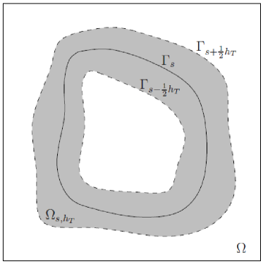
1. for a fixed value of the state variable $s=T_{i}$ we define the interval $[T_{i-\frac{1}{2}},T_{i+\frac{1}{2}}]=[s-\frac{1}{2}h_{T},s+\frac{1}{2}h_{T}]\subset{\mathcal{L}}$; then, we have

   $$f(s)\approx\frac{1}{h_{T}}\int_{s-\frac{1}{2}h_{T}}^{s+\frac{1}{2}h_{T}}f(\zeta)\,d\zeta,$$ (50)

2. now we define a subdomain $\Omega_{s,h_{T}}\subset\Omega$ which contains all the points of $\Omega$ that lie between the two level–set curves $\Gamma_{s-\frac{1}{2}h_{T}}$ and $\Gamma_{s+\frac{1}{2}h_{T}}$

   $$\Omega_{s,h_{T}}\triangleq\left\{{\bf x}\in\Omega,\,T({\bf x})\in\left[s-\frac{1}{2}h_{T},s+\frac{1}{2}h_{T}\right]\right\},$$ (51)

   see Figure 2a; we then approximate $\Omega_{s,h_{T}}$ with the region

   $$\tilde{\Omega}_{s,h_{T}}\triangleq\bigcup^{N_{s,h_{T}}}_{j=1}\Omega^{\square}_{s,h_{T};j},\quad\textrm{where}\ \ \Omega^{\square}_{s,h_{T};j}=\left\{\Omega^{\square}_{j}\;:\;{\bf x}^{0}_{j}\in\Omega^{\square}_{j}\ \textrm{and}\ T({\bf x}^{0}_{j})\in\left[s-\frac{1}{2}h_{T},s+\frac{1}{2}h_{T}\right]\right\},$$ (52)

   see Figure 2b, which consists of the quadrilateral finite elements $\Omega^{\square}_{s,h_{T};j}$, $j=1,\dots,N_{s,h_{T}}$, with the center points ${\bf x}^{0}_{j}$ satisfying the condition $T({\bf x}^{0}_{j})\in[s-(1/2)h_{T},s+(1/2)h_{T}]$,

3. in view of (50), expression (37) is approximated with an area integral over the region contained between the level–set curves $\Gamma_{s-\frac{1}{2}h_{T}}$ and $\Gamma_{s+\frac{1}{2}h_{T}}$, which is in turn approximated by the FEM region $\tilde{\Omega}_{s,h_{T}}$ given by (52); finally, the integral over this region is approximated using the standard 2D compound midpoint rule as

   $$f(s)\approx\frac{1}{h_{T}}\int_{s-\frac{1}{2}h_{T}}^{s+\frac{1}{2}h_{T}}\int_{\Omega}\delta(s({\bf x})-\zeta)g({\bf x})\,d{\bf x}\,d\zeta\approx\dfrac{h^{2}}{h_{T}}\sum_{j=1}^{N_{s,h_{T}}}g({\bf x}^{0}_{j}).$$ (53)

As regards the accuracy of this approach, we have the following

Theorem 6.1.

Formula (53) is second order accurate with respect to the discretization of the space domain and first order accurate with respect to the discretization of the state domain, i.e.,

$$f(s)=\int_{\Omega}\delta(T({\bf x})-s)g({\bf x})\ d{\bf x}=\dfrac{h^{2}}{h_{T}}\sum_{j=1}^{N_{s,h_{T}}}g({\bf x}^{0}_{j})+{\mathcal{O}}(h^{2})+{\mathcal{O}}(h_{T}).$$ (54)

Proof.

We start by integrating both sides of (37) over the interval $[T_{i-\frac{1}{2}};T_{i+\frac{1}{2}}]=[s-\frac{1}{2}h_{T};s+\frac{1}{2}h_{T}]$ obtaining

$$\int_{s-\frac{1}{2}h_{T}}^{s+\frac{1}{2}h_{T}}f(\zeta)\ d\zeta=\int_{\Omega}\left[\int_{s-\frac{1}{2}h_{T}}^{s+\frac{1}{2}h_{T}}\delta(T({\bf x})-\zeta)\ d\zeta\right]g({\bf x})\ d{\bf x}=\int_{\Omega}\chi_{[s-\frac{1}{2}h_{T},s+\frac{1}{2}h_{T}]}(T({\bf x}))\ g({\bf x})\ d{\bf x},$$ (55)

where the characteristic function

$$\chi_{[T^{\prime},T^{\prime\prime}]}(T({\bf x}))=\left\{\begin{aligned} &1\quad&&\textrm{for}\ T({\bf x})\in[T^{\prime},T^{\prime\prime}],\\ &0&&\textrm{for}\ T({\bf x})\notin[T^{\prime},T^{\prime\prime}]\end{aligned}\right.$$

describes the subdomain $\Omega_{s,h_{T}}$ introduced earlier in (51), cf. Figure 2a. Now, using a second–order accurate midpoint rule for 1D integration, we can express the LHS of (55) as

$$\int_{s-\frac{1}{2}h_{T}}^{s+\frac{1}{2}h_{T}}f(\zeta)\ d\zeta=f\left(\dfrac{T_{i-\frac{1}{2}}+T_{i+\frac{1}{2}}}{2}\right)\cdot h_{T}+{\mathcal{O}}(h_{T}^{2})=f(s)h_{T}+{\mathcal{O}}(h_{T}^{2}).$$ (56)

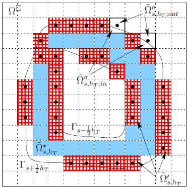
Approximation of the RHS in (55) takes place in two steps. In the first step we approximate the actual integration domain $\Omega_{s,h_{T}}$ with the union of the finite elements $\tilde{\Omega}_{s,h_{T}}$, cf. (52). In order to estimate the error

$$E_{1}\triangleq\left|\int_{\Omega_{s,h_{T}}}g({\bf x})\ d{\bf x}-\int_{\tilde{\Omega}_{s,h_{T}}}g({\bf x})\ d{\bf x}\right|$$

of this step, we divide the set of cells $\tilde{\Omega}_{s,h_{T}}$ into two subsets, see Figure 2b,

$$\tilde{\Omega}_{s,h_{T}}=\tilde{\Omega}^{*}_{s,h_{T}}\cup\tilde{\Omega}^{\prime}_{s,h_{T}},$$

where $\tilde{\Omega}^{*}_{s,h_{T}}$ consists of the cells with all 4 vertices $\{{\bf x}_{k}\}_{k=1}^{4}$ satisfying the condition $T({\bf x}_{k})\in[s-\frac{1}{2}h_{T},s+\frac{1}{2}h_{T}]$. The subregion $\tilde{\Omega}^{\prime}_{s,h_{T}}$, defined as the compliment of $\tilde{\Omega}^{*}_{s,h_{T}}$ in $\tilde{\Omega}_{s,h_{T}}$, represents the union of “truncated” cells, i.e., cells which have at least one node outside $\Omega_{s,h_{T}}$. This subregion is in turn further subdivided into two subsets, i.e.,

$$\tilde{\Omega}^{\prime}_{s,h_{T}}=\tilde{\Omega}^{\prime}_{s,h_{T};in}\cup\tilde{\Omega}^{\prime}_{s,h_{T};out},$$

where

$$\tilde{\Omega}^{\prime}_{s,h_{T};in}\triangleq\left\{{\bf x}\in\tilde{\Omega}^{\prime}_{s,h_{T}},\,T({\bf x})\in\left[s-\frac{1}{2}h_{T},s+\frac{1}{2}h_{T}\right]\right\},$$

$$\tilde{\Omega}^{\prime}_{s,h_{T};out}\triangleq\left\{{\bf x}\in\tilde{\Omega}^{\prime}_{s,h_{T}},\,T({\bf x})\notin\left[s-\frac{1}{2}h_{T},s+\frac{1}{2}h_{T}\right]\right\}.$$

We have to define one more set $\tilde{\Omega}^{\prime\prime}_{s,h_{T}}$ which consists of the cells with at least one vertex $\{{\bf x}_{k}\}_{k=1}^{4}$ satisfying the condition $T({\bf x}_{k})\in[s-\frac{1}{2}h_{T},s+\frac{1}{2}h_{T}]$, but whose center points ${\bf x}^{0}_{j}$ lie outside $\Omega_{s,h_{T}}$. We also further subdivide this set into two subsets

$$\tilde{\Omega}^{\prime\prime}_{s,h_{T}}=\tilde{\Omega}^{\prime\prime}_{s,h_{T};in}\cup\tilde{\Omega}^{\prime\prime}_{s,h_{T};out},$$

where

$$\tilde{\Omega}^{\prime\prime}_{s,h_{T};in}\triangleq\left\{{\bf x}\in\tilde{\Omega}^{\prime\prime}_{s,h_{T}},\,T({\bf x})\in\left[s-\frac{1}{2}h_{T},s+\frac{1}{2}h_{T}\right]\right\},$$

$$\tilde{\Omega}^{\prime\prime}_{s,h_{T};out}\triangleq\left\{{\bf x}\in\tilde{\Omega}^{\prime\prime}_{s,h_{T}},\,T({\bf x})\notin\left[s-\frac{1}{2}h_{T},s+\frac{1}{2}h_{T}\right]\right\}.$$

We thus have

$$\int_{\Omega_{s,h_{T}}}g({\bf x})\ d{\bf x}=\int_{\tilde{\Omega}^{*}_{s,h_{T}}}g({\bf x})\ d{\bf x}+\int_{\tilde{\Omega}^{\prime}_{s,h_{T};in}}g({\bf x})\ d{\bf x}+\int_{\tilde{\Omega}^{\prime\prime}_{s,h_{T};in}}g({\bf x})\ d{\bf x},$$ (57)

$$\int_{\tilde{\Omega}_{s,h_{T}}}g({\bf x})\ d{\bf x} =\int_{\tilde{\Omega}^{*}_{s,h_{T}}}g({\bf x})\ d{\bf x}+\int_{\tilde{\Omega}^{\prime}_{s,h_{T}}}g({\bf x})\ d{\bf x}$$ (58)

$$=\int_{\tilde{\Omega}^{*}_{s,h_{T}}}g({\bf x})\ d{\bf x}+\int_{\tilde{\Omega}^{\prime}_{s,h_{T};in}}g({\bf x})\ d{\bf x}+\int_{\tilde{\Omega}^{\prime}_{s,h_{T};out}}g({\bf x})\ d{\bf x},$$

so that the domain approximation error can be estimated as follows

$$E_{1}=\left|\int_{\tilde{\Omega}^{\prime}_{s,h_{T};out}}g({\bf x})\ d{\bf x}-\int_{\tilde{\Omega}^{\prime\prime}_{s,h_{T};in}}g({\bf x})\ d{\bf x}\right| \leq\left|\int_{\tilde{\Omega}^{\prime}_{s,h_{T};out}}g({\bf x})\ d{\bf x}\right|+\left|\int_{\tilde{\Omega}^{\prime\prime}_{s,h_{T};in}}g({\bf x})\ d{\bf x}\right|$$ (59)

$$\leq\max_{{\bf x}\in\Omega}|g({\bf x})|\ \left(\left|\tilde{\Omega}^{\prime}_{s,h_{T}}\right|+\left|\tilde{\Omega}^{\prime\prime}_{s,h_{T}}\right|\right)={\mathcal{O}}(h^{2}),$$

where $|\Omega|\triangleq\textrm{meas}\ \Omega$. The second error in the approximation of the RHS of (55) is related to the accuracy of the quadrature applied to $\int_{\tilde{\Omega}_{s,h_{T}}}g({\bf x})\ d{\bf x}$ and for the 2D compound midpoint rule is $E_{2}={\mathcal{O}}(h^{2})$, so that we obtain

$$\left|\int_{\tilde{\Omega}_{s,h_{T}}}g({\bf x})\,d{\bf x}-\sum_{j=1}^{N_{s,h_{T}}}g({\bf x}^{0}_{j})\,h^{2}\right|={\mathcal{O}}(h^{2}).$$ (60)

Comparing (53) with (56) and dividing both sides into $h_{T}$ we finally obtain (54) which completes the proof. ∎

Figure 2: Illustration of approach #3 where line integral (37) is approximated with an area integral (see Section 6.3): (a) region $\Omega_{s,h_{T}}$ which lies between the two level–set curves $\Gamma_{s-\frac{1}{2}h_{T}}$ and $\Gamma_{s+\frac{1}{2}h_{T}}$ and (b) its approximation with the region $\tilde{\Omega}_{s,h_{T}}=\tilde{\Omega}^{*}_{s,h_{T}}\cup\tilde{\Omega}^{\prime}_{s,h_{T}}$, where checked cells represent $\tilde{\Omega}^{\prime}_{s,h_{T}}$ and shaded cells represent $\tilde{\Omega}^{*}_{s,h_{T}}$. Figure (b) also shows a part of the region $\tilde{\Omega}^{\prime\prime}_{s,h_{T}}=\tilde{\Omega}^{\prime\prime}_{s,h_{T};in}\cup\tilde{\Omega}^{\prime\prime}_{s,h_{T};out}$ represented by 2 elements in the top right corner.

So far, we have considered the discretizations of the physical and state spaces, $\Omega$ and ${\mathcal{L}}$, as independent. We remark that using the relationship

$$\min_{{\bf x}\in\Omega}|\boldsymbol{\nabla}T({\bf x})|\cdot h\leq h_{T}\leq\max_{{\bf x}\in\Omega}|\boldsymbol{\nabla}T({\bf x})|\cdot h$$ (61)

one could link the corresponding discretization parameters $h$ and $h_{T}$ to each other.

7 Computational Results

7.1 Comparison of Different Approaches to Gradient Evaluation

In this Section we discuss the accuracy and efficiency of the three methods for evaluation of expression (37) presented in Sections 6.1, 6.2 and 6.3. In order to assess their utility for the parameter reconstruction problem studied in this work, we will consider the following three test cases

1. single (fixed) value of $s$ with $\phi(s,{\bf x})$ and $g({\bf x})$ given analytically,

2. parameter $s$ varying over a finite range with $\phi(s,{\bf x})$ and $g({\bf x})$ given analytically,

3. parameter $s$ varying over a finite range with $\phi(s,{\bf x})$ and $g({\bf x})$ given in terms of solutions of the direct and adjoint problem.

Tests (ii) and (iii) with $s$ spanning the entire interval ${\mathcal{L}}$ are particularly relevant for the present reconstruction problem, as they help us assess the accuracy of the cost functional gradients over their entire domains of definition, including the values of $s$ for which the level sets $\Gamma_{s}$ intersect the domain boundary $\partial\Omega$. Results of tests (i)–(iii) are presented below.

7.1.1 Tests for a Single Value of $s$ with $\phi(s,{\bf x})$ and $g({\bf x})$ Given Analytically

Here we employ our three methods to compute numerically the value of a line integral over the circle $x^{2}+y^{2}=1$

1. in domain $\Omega_{1}=[-2,2]^{2}$ which contains the entire curve

   $$I_{ex,1}=\int_{x^{2}+y^{2}=1}(3x^{2}-y^{2})\ d\sigma=2\pi$$ (62)

   (this test problem is actually borrowed from [11]),

2. and in domain $\Omega_{2}=[0,2]^{2}$ which contains only a part of the curve in the first quadrant

   $$I_{ex,2}=\int_{x^{2}+y^{2}=1,\,x,y>0}(3x^{2}-y^{2})\ d\sigma=\frac{\pi}{2}.$$ (63)

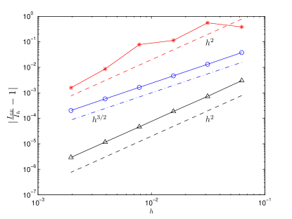
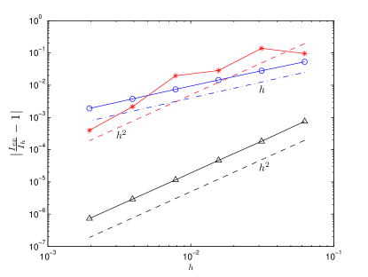
The main difference between test cases (a) and (b) is that while in (a) the contour is entirely contained in the domain $\Omega_{1}$, it intersects the domain boundary $\partial\Omega_{2}$ in case (b). As shown in Figure 3, methods #1 (line integration) and #3 (area integration) in both cases show the expected accuracy of ${\mathcal{O}}(h^{2})$, where $h=\Delta x=\Delta y=2^{-(3+i)}$, $i=1\dots 6$, while method #2 (delta function approximation) is ${\mathcal{O}}(h^{3/2})$ accurate in case (a) and only ${\mathcal{O}}(h^{1})$ accurate in case (b). We also add that the line integration method exhibits the smallest constant prefactor characterizing the error.

 

Figure 3: Relative error $|\frac{I_{ex,i}}{I_{h}}-1|$, $i=1,2$, versus discretization step $h=\Delta x=\Delta y$ in the numerical approximation $I_{h}$ of (a) line integral (62) and (b) line integral (63), see Section 7.1.1. Triangles represent the line integration approach (method #1), circles represent the results obtained using the delta function approximation (method #2), whereas asterisks show the data for the area integration approach (method #3).

7.1.2 Tests for $s$ Varying Over a Finite Range with $\phi(s,{\bf x})$ and $g({\bf x})$ Given Analytically

In order to analyze this case we will introduce a new diagnostic quantity. We begin with the integral transform formula (28) applied to some perturbation $\mu^{\prime}(T({\bf x}))$

$$\mu^{\prime}(T({\bf x}))=\int_{-\infty}^{+\infty}\delta(\phi(s,{\bf x}))\mu^{\prime}(s)\,ds,$$ (64)

where $\phi(s,{\bf x})=T({\bf x})-s$. Multiplying both sides of (64) by $g({\bf x})$, integrating over the domain $\Omega$ and changing the order of integration we obtain the following useful identity

$$\int_{\Omega}\mu^{\prime}(T({\bf x}))g({\bf x})\,d{\bf x}=\int_{-\infty}^{+\infty}f(s)\mu^{\prime}(s)\,ds$$ (65)

with $f(s)$ defined in (37), where the RHS has the structure of the Riesz identity for the Gâteaux differential of the cost functional, cf. (30), whereas the LHS is a simple area integral which can be easily evaluated using high–accuracy quadratures. Given the formal similarity of the RHS of (65) and the Riesz formula (30), this test is quite relevant for the optimization problem we are interested in here. We will thus use our three methods to evaluate the RHS of (65) and compared it to the LHS, which is evaluated with high precision on a refined grid in $\Omega$, so that it can be considered “exact”. Our tests are based on the following data

• spatial domain $\Omega=[0,1]^{2}$ discretized with $h=\Delta x=\Delta y=2^{-(4+i)}$, $i=1\dots 7$,

• state domain ${\mathcal{L}}=[T_{a},T_{b}]$, where $T_{a}=100$, $T_{b}=700$, discretized using $N_{T}=200,1000,10000$ points for methods #2 and #3 and $N_{T}=200,2000,20000$ points for method #1; $h_{T}=\dfrac{T_{b}-T_{a}}{N_{T}}$,

• $T({\bf x})=100(x^{2}+y^{2})+300$,   $g({\bf x})=\cos(x)+3\sin(2y-1)$, ${\bf x}\in\Omega$,

• perturbations used $\mu^{\prime}_{1}(s)=\exp(-\frac{s}{1000})$, $\mu^{\prime}_{2}(s)=\frac{10}{s^{2}}$ and $\mu^{\prime}_{3}(s)=-\frac{s^{2}}{90000}+\frac{2s}{225}+\frac{2}{9}$, $s\in[T_{a},T_{b}]$.

Figure 4: Relative error $|\xi-1|$, where $\xi=\frac{\textrm{LHS of \eqref{eq:test2_int}}}{\textrm{RHS of \eqref{eq:test2_int}}}$, versus discretization step $h=\Delta x=\Delta y$ in approximating the RHS in (65). The first, second and third row of figures show the results for $\mu^{\prime}_{1}$, $\mu^{\prime}_{2}$ and $\mu^{\prime}_{3}$, respectively, while the figures in the first, second and third column represent line integration (#1), delta function approximation (#2) and area integration (#3) methods, respectively.

Figure 5: Relative error $|\xi-1|$, where $\xi=\frac{\textrm{LHS of \eqref{eq:test2_int}}}{\textrm{RHS of \eqref{eq:test2_int}}}$, versus discretization step $h_{T}$ in the state space ${\mathcal{L}}$ in approximating the RHS in (65). The first, second and third row of figures show the results for $\mu^{\prime}_{1}$, $\mu^{\prime}_{2}$ and $\mu^{\prime}_{3}$, respectively, while the figures in the first, second and third column represent line integration (#1), delta function approximation (#2) and area integration (#3) methods, respectively.

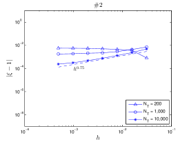
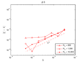
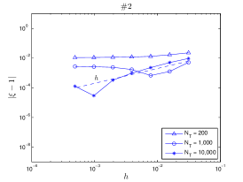
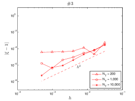
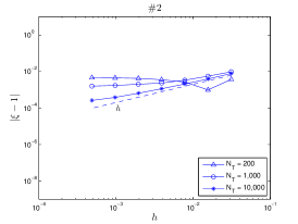
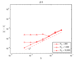
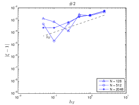
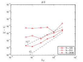
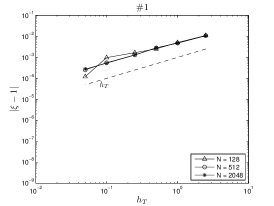
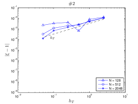
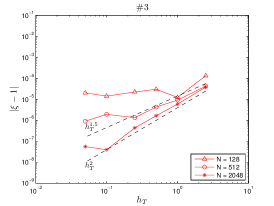
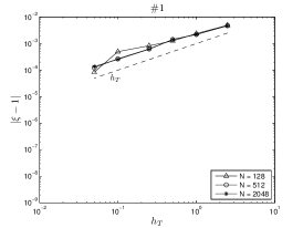
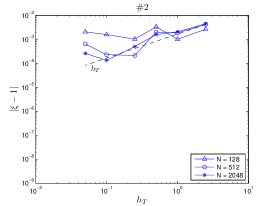
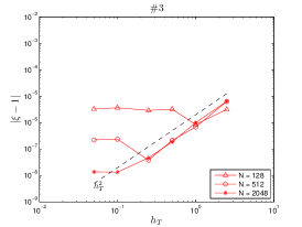
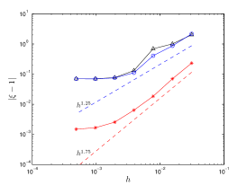
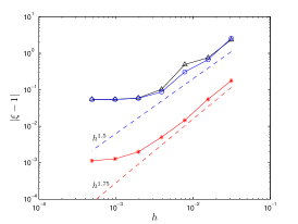
As is evident from Figure 4, all three methods show similar qualitative behavior, namely, the error decreases with decreasing $h$ until it saturates which is due to the error terms depending on $h_{T}$ becoming dominant. The saturation value of the error depends on the state space resolution $h_{T}$ and is different for the different methods. Method #3 (area integration) reveals accuracy ${\mathcal{O}}(h^{2})$, whereas method #2 (delta function approximation) is again only of accuracy about ${\mathcal{O}}(h)$ for the same discretization of the interval ${\mathcal{L}}$. Method #1 (line integration) performs better and shows accuracy up to ${\mathcal{O}}(h^{5})$, but requires much finer resolution in the state space, namely $N_{T}>20000$ ($h_{T}<0.03$) is needed for this behavior to be visible. On the other hand, method #3 (area integration) leads to the smallest errors for all the cases tested.

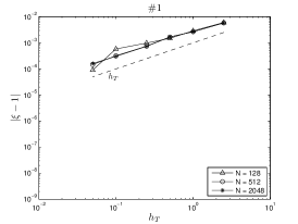
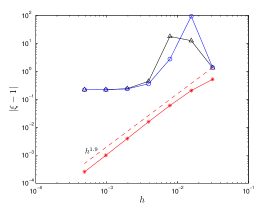
Analogous data is plotted in Figure 5 now as a function of the state space resolution $h_{T}$ with $h$ acting as a parameter. Similar trends are observed as in Figure 4, namely, the errors decrease with $h_{T}$ until they eventually saturate when the error terms depending on $h$ become dominant. Methods #1 and #2 reveal accuracy ${\mathcal{O}}(h_{T})$, whereas method #3 has accuracy ${\mathcal{O}}(h_{T}^{1.5\div 2})$ which is actually better than stipulated by Theorem 54, cf. (54). Method #3 is also characterized by the smallest value of the constant prefactor leading to the smallest overall errors.

7.1.3 Tests for $s$ Varying Over a Finite Range with $\phi(s,{\bf x})$ and $g({\bf x})$ Given by Solutions of Direct and Adjoint Problem

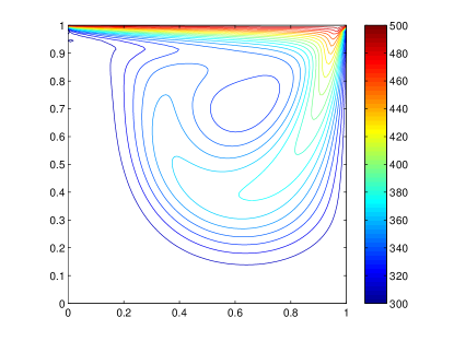
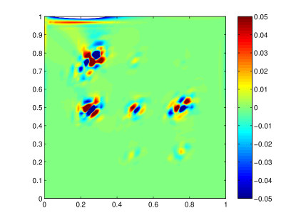
We now repeat the test described in Section 7.1.2 using $\phi(s,{\bf x})=T({\bf x})-s$ and $g({\bf x})=[\boldsymbol{\nabla}{\bf u}({\bf x})+(\boldsymbol{\nabla}{\bf u}({\bf x}))^{T}]:\boldsymbol{\nabla}{\bf u}^{*}({\bf x})$, where the fields ${\bf u}$, $T$ and ${\bf u}^{*}$ come from the solutions of the direct and adjoint problem (1)–(2) and (18)–(19) at some fixed time $t$, see Figure 6 (details of these computations will be given in Section 7.5). As before, we discretize the domain $\Omega=[0,1]^{2}$ with the step $h=\Delta x=\Delta y=2^{-(4+i)}$, $i=1\dots 7$, and the state space ${\mathcal{L}}=[T_{a},T_{b}]$, $T_{a}=100$ and $T_{b}=700$, with the step $h_{T}=0.06$ ($N_{T}=10000$).

Figure 6: The fields (a) $T({\bf x})$ (level set contours) and (b) $g({\bf x})=[\boldsymbol{\nabla}{\bf u}({\bf x})+(\boldsymbol{\nabla}{\bf u}({\bf x}))^{T}]:\boldsymbol{\nabla}{\bf u}^{*}({\bf x})$ obtained at some time $t$ by solving (1)–(2) and (18)–(19).

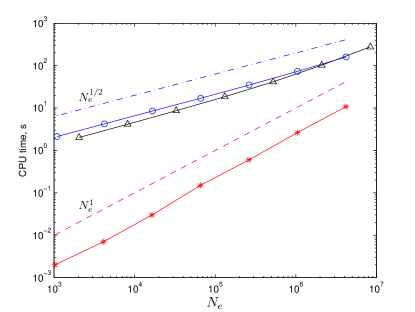
The data shown in Figure 7 confirms our findings from Sections 7.1.1 and 7.1.2, namely, that in this case as well the error of all three methods decreases with $h$ until it eventually saturates when the errors depending on $h_{T}$ become dominant. Method #3 is again characterized by the smallest prefactor and hence leads to much smaller overall errors than in methods #1 and #2. The computational complexity of our three approaches is addressed in Figure 8, where $N_{e}$ is defined as a number of computational elements, i.e., $N_{e}=N_{\triangle}$, or $N_{e}=N_{\square}$, using (40) or (41), respectively. We see that, while the complexity of methods #1 and #2 scales as ${\mathcal{O}}(\sqrt{N_{e}})$, method #3 exhibits the scaling of ${\mathcal{O}}(N_{e})$. On the other hand, however, method #3 has the smallest prefactor and, at least in the range of resolutions considered here, results in the shortest execution time.

In conclusion, these observations make the area integration approach (method #3) the method of choice for the present parameter reconstruction problem, and this is the approach we will use in all subsequent computations.

Figure 7: Relative error $|\xi-1|$, where $\xi=\frac{\textrm{LHS of \eqref{eq:test2_int}}}{\textrm{RHS of \eqref{eq:test2_int}}}$, versus discretization step $h=\Delta x=\Delta y$ in estimating the RHS in (65), where $\phi(s,{\bf x})=T({\bf x})-s$, and $g({\bf x})=[\boldsymbol{\nabla}{\bf u}+(\boldsymbol{\nabla}{\bf u})^{T}]:\boldsymbol{\nabla}{\bf u}^{*}$ is obtained by solving (1)–(2) and (18)–(19). Figures (a), (b) and (c) show the results for $\mu^{\prime}_{1}$, $\mu^{\prime}_{2}$ and $\mu^{\prime}_{3}$, respectively, using the same discretization of the state space ${\mathcal{L}}$ with $N_{T}=10000$. Triangles represent the line integration approach (#1), circles show the results for the method of the delta function approximation (#2), while asterisks show the data from the area integration approach (#3).

Figure 8: CPU time (in seconds) versus the number $N_{e}$ of computational elements used in the different approaches, namely, (triangles) finite elements $\Omega^{\vartriangle}_{i}$ in the line integration approach (method #1), (circles) grid nodes in the method of the delta function approximation (#2) and (asterisks) finite elements $\Omega^{\square}_{i}$ in the area integration approach (#3). The data shown corresponds to the estimation of the RHS in (65) for $\mu^{\prime}_{1}$ using the same discretization of the state space with $N_{T}=10000$, $\phi(s,{\bf x})=T({\bf x})-s$ and $g({\bf x})=[\boldsymbol{\nabla}{\bf u}+(\boldsymbol{\nabla}{\bf u})^{T}]:\boldsymbol{\nabla}{\bf u}^{*}$ obtained by solving (1)–(2) and (18)–(19).

7.2 Models for Constitutive Relations

For validation purposes one needs an algebraic expression to represent the dependence of the viscosity coefficient on temperature which could serve as the “true” material property we will seek to reconstruct. The dynamic viscosity in liquids is usually approximated by exponential relations [34] and one of the most common expression for the coefficient of the dynamic viscosity is the law of Andrade (also referred to as the Nahme law) which is given in the dimensional form valid for $T$ expressed in Kelvins in (66) below

$$\tilde{\mu}(T)=C_{1}e^{C_{2}/T},$$ (66)

where $C_{1},\ C_{2}>0$ are constant parameters. As regards the thermal conductivity $k$, since it typically reveals a rather weak dependence on the temperature, for the sake of simplicity we will treat it as a constant setting $k=0.002$ in all computations presented in this paper.

7.3 Model Geometry and PDE Solvers

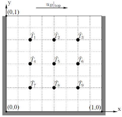
To validate the accuracy and performance of the proposed approach to reconstruct $\mu(T)$, we use a simple 2D lid–driven (shear–driven) cavity flow, cf. Figure 9, as our model problem. Due to the simplicity of its geometry and boundary conditions, the lid–driven cavity flow problem has been used for a long time to validate novel solution approaches and codes [35, 36]. Numerical results are available for different aspect ratios and the problem was solved in both laminar and turbulent regimes using different numerical techniques. Thus, this problem is a useful testbed as there is a great deal of numerical data that can be used for comparison. Our code for solving direct problem (1)–(2) and adjoint problem (18)–(19) has been implemented using FreeFem++ [37], an open–source, high–level integrated development environment for the numerical solution of PDEs based on the the Finite Element Method. The direct solver has been thoroughly validated against available benchmark data from [35, 36], and all details are reported in [31].

Figure 9: Geometry of the 2D lid-driven (shear-driven) cavity.

To solve numerically the direct problem we discretize system (1)–(2) in time using a second–order accurate semi-implicit approach. Spatial discretization is carried out using triangular finite elements (40) and the P2 piecewise quadratic (continuous) representations for the velocity ${\bf u}$ and the temperature $T$ fields, and the P1 piecewise linear (continuous) representation for the pressure $p$ field. The system of algebraic equations obtained after such discretization is solved at every time step with UMFPACK, a solver for nonsymmetric sparse linear systems [38]. We add that incompressibility is ensured by an implicit treatment of equation (1b). Stability is enforced by choosing the time step $\Delta t$ so that it satisfies the following CFL condition

$$\left|\Delta t\left(\frac{\max_{{\bf x}\in\Omega}u({\bf x})}{h_{x}}+\frac{\max_{{\bf x}\in\Omega}v({\bf x})}{h_{y}}\right)\right|\leq 1.$$ (67)

The same technique is used for the numerical solution of adjoint problem (18)–(19).

All our computations are performed using a 2D square domain $\Omega=[0,1]^{2}$ shown in Figure 9. Governing system (1)–(2) and adjoint system (18)–(19) are discretized on a uniform mesh with $N=N_{x}=N_{y}=32$ grid points in every direction using triangular finite elements combined with the cubic spline interpolation of the function $\mu(T({\bf x}))$. The rather modest spatial resolution used is a consequence of the fact that in a single reconstruction problem the governing and adjoint systems need to be solved ${\mathcal{O}}(10^{3}-10^{4})$ times, hence there are limitations of the computational time. Unless stated otherwise, the interval ${\mathcal{L}}=[100.0,700.0]$ is discretized using an equispaced grid with $N_{T}=600$ points. The actual constitutive relation $\tilde{\mu}(T)$ we seek to reconstruct is given by Andrade law (66) with $C_{1}=0.001$ and $C_{2}=10^{3}$. In the computational tests reported below we used $M=9$ measurement points distributed uniformly inside the cavity (Figure 9). To mimic an actual experimental procedure, first relation (66) is used in combination with governing system (1)–(2) to obtain pointwise temperature measurements $\{\tilde{T}_{i}\}_{i=1}^{M}$. Relation (66) is then “forgotten” and is reconstructed using gradient–based algorithm (14). In terms of the initial guess in (14), unless stated otherwise, we take a constant approximation $\mu_{0}$ to (66), given by $\mu_{0}=\frac{1}{2}\left(\tilde{\mu}(T_{\alpha})+\tilde{\mu}(T_{\beta})\right)=\frac{C_{1}}{2}\left(e^{C_{2}/T_{\alpha}}+e^{C_{2}/T_{\beta}}\right)$ which translates into the following expression for the new optimization variable $\theta$, cf. (8), $\theta_{0}=\sqrt{\mu_{0}-m_{\mu}}$, where $m_{\mu}=\frac{1}{2}\tilde{\mu}(T_{\beta})=\frac{C_{1}}{2}e^{C_{2}/T_{\beta}}$. Since in the present problem the viscosity $\mu(T)$ is a function of the temperature, the Reynolds number is defined locally (both in space and in time) and varies in the range $Re=0.05\div 240$.

Unless stated otherwise, the boundary conditions for the temperature are $T_{B}|_{\textrm{top}}=T_{\beta}=500$ and $T_{B}|_{\textrm{else}}=T_{\alpha}=300$ which results in the identifiability region ${\mathcal{I}}=[300.0,500.0]$. The velocity boundary conditions ${\bf u}_{B}=[u_{B},v_{B}]^{T}$ are given by $u_{B}|_{\textrm{top}}=U_{0}\cos(2\pi t)$, $U_{0}=1$ and $v_{B}|_{\textrm{top}}=0$ on the top boundary segment and ${\bf u}_{B}|_{\textrm{else}}={\bf 0}$ on the remaining boundary segments. Their time–dependent character ensures that the obtained flow is unsteady at the values of the Reynolds number for which self–sustained oscillations do not spontaneously occur (the study of higher Reynolds numbers was restricted by the numerical resolution used, see comments above). The initial conditions $\{{\bf u}_{0},T_{0}\}$ used in the reconstruction problem correspond to a developed flow obtained at $t=10$ from the following initial and boundary conditions $T_{B}|_{\textrm{top}}=500$, $T_{B}|_{\textrm{else}}=300$ and $u_{B}|_{\textrm{top}}=1$, $v_{B}|_{\textrm{top}}=0$, ${\bf u}_{B}|_{\textrm{else}}={\bf 0}$, $T_{0}=300$, ${\bf u}_{0}={\bf 0}$. We emphasize that adjoint system (18)–(19) is in fact a terminal–value problem which needs to be integrated backwards in time, and its coefficients depend on the solution $\{{\bf u},T\}$ of the direct problem around which linearization is performed at the given iteration. Our reconstructions are performed using the following time windows $[0,t_{f}]$, $t_{f}=\left\{\frac{1}{4},\frac{1}{2},1\right\}$ which correspond to a fraction of, or a full, forcing cycle in the boundary conditions described above. These time windows are all discretized with the time step $\Delta t=5\cdot 10^{-3}$ in both the direct and adjoint problems. This choice of the time step $\Delta t$ ensures stability by satisfying the CFL condition (67).

7.4 Validation of Gradients

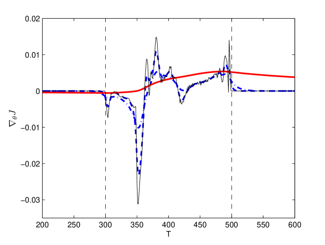
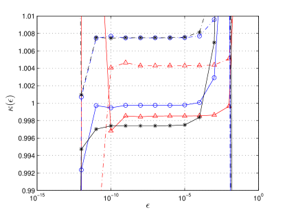
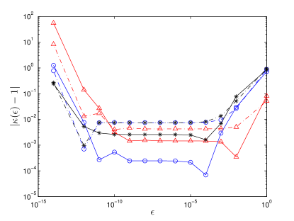
In this Section we present results demonstrating the consistency of the cost functional gradients obtained with the approach described in Section 4. In Figure 10 we present the $L_{2}$ and several Sobolev $H^{1}$ gradients obtained at the first iteration. In the first place, we observe that, as was anticipated in Section 4, the $L_{2}$ gradients indeed exhibit quite irregular behaviour lacking necessary smoothness which makes them unsuitable for the reconstruction of constitutive relations with required properties, cf. (10). On the other hand, the gradients extracted in the Sobolev space $H^{1}$ are characterized by the required smoothness and therefore hereafter we will solely use the Sobolev gradients. Next, in Figure 11 we present the results of a diagnostic test commonly employed to verify the correctness of the cost functional gradient [39]. It consists in computing the directional Gâteaux differential ${\mathcal{J}}^{\prime}(\theta;\theta^{\prime})$ for some selected perturbations $\theta^{\prime}$ in two different ways, namely, using a finite–difference approximation and using (29) which is based on the adjoint field, and then examining the ratio of the two quantities, i.e.,

$$\kappa(\epsilon)\triangleq\dfrac{\epsilon^{-1}\left[{\mathcal{J}}(\theta+\epsilon\theta^{\prime})-{\mathcal{J}}(\theta)\right]}{\int_{-\infty}^{+\infty}\boldsymbol{\nabla}_{\theta}{\mathcal{J}}(s)\,\theta^{\prime}(s)\,ds}$$ (68)

for a range of values of $\epsilon$. If the gradient $\boldsymbol{\nabla}_{\theta}{\mathcal{J}}(\theta)$ is computed correctly, then for intermediate values of $\epsilon$, $\kappa(\epsilon)$ will be close to the unity. Remarkably, this behavior can be observed in Figure 11 over a range of $\epsilon$ spanning about 6 orders of magnitude for three different perturbations $\theta^{\prime}(T)$. Furthermore, we also emphasize that refining the time step $\Delta t$ used in the time–discretization of (1)–(2) and (18)–(19) yields values of $\kappa(\epsilon)$ closer to the unity. The reason is that in the “optimize–then–discretize” paradigm adopted here such refinement of discretization leads to a better approximation of the continuous gradient (29). We add that the quantity $\log_{10}|\kappa(\epsilon)-1|$ plotted in Figure 11b shows how many significant digits of accuracy are captured in a given gradient evaluation. As can be expected, the quantity $\kappa(\epsilon)$ deviates from the unity for very small values of $\epsilon$, which is due to the subtractive cancellation (round–off) errors, and also for large values of $\epsilon$, which is due to the truncation errors, both of which are well–known effects.

Figure 10: Comparison of (thin solid line) the $L_{2}$ gradient $\boldsymbol{\nabla}^{L_{2}}_{\theta}{\mathcal{J}}$ and the Sobolev gradients $\boldsymbol{\nabla}^{H^{1}}_{\theta}{\mathcal{J}}$ defined in (31) for different values of the smoothing coefficient (thick dashed line) $\ell=2.5$, (thick dash–dotted line) $\ell=10.0$ and (thick solid line) $\ell=200.0$ at the first iteration with the initial guess $\mu_{0}=const=0.0177$. The vertical dashed lines represent the boundaries of the identifiability interval ${\mathcal{I}}$ and the vertical scale in the plot is arbitrary.

Figure 11: The behavior of (a) $\kappa(\epsilon)$ and (b) $\log_{10}|\kappa(\epsilon)-1|$ as a function of $\epsilon$ for different perturbations (triangles) $\theta^{\prime}(T)=\frac{10}{T}$, (circles) $\theta^{\prime}(T)=e^{-\frac{T}{1000}}$ and (asterisks) $\theta^{\prime}(T)=-\frac{T^{2}}{90000}+\frac{2T}{225}+\frac{2}{9}$. The time steps used in the time integration of (1)–(2) and (18)–(19) are (dash–dotted line) $\Delta t=5.0\cdot 10^{-3}$ and (solid line) $\Delta t=5.0\cdot 10^{-4}$.

7.5 Reconstruction Results

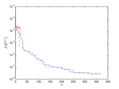
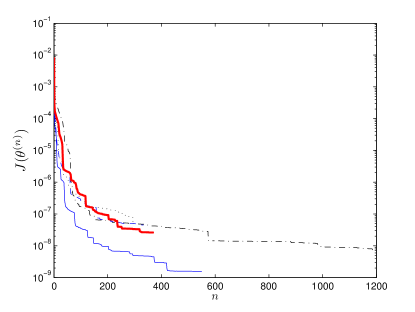
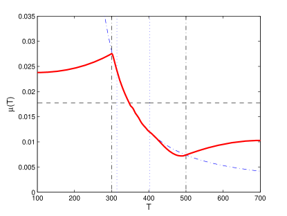
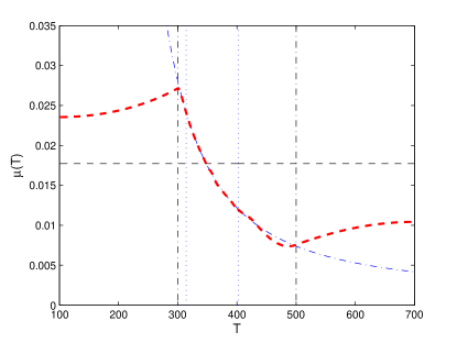
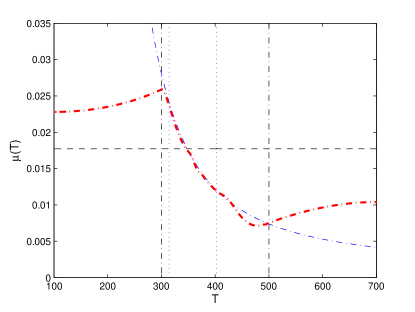
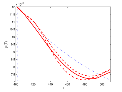
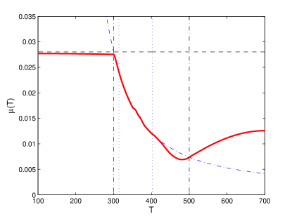
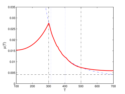
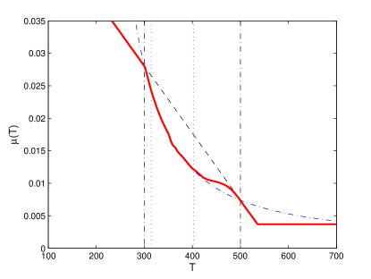
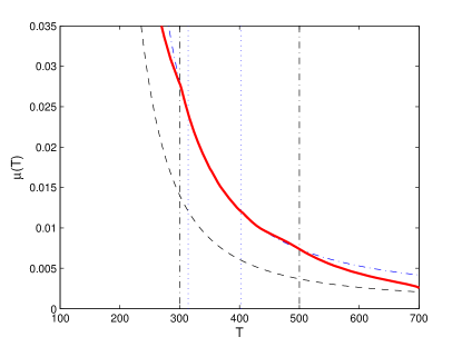
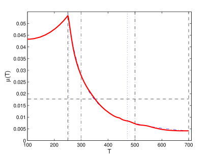
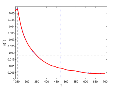
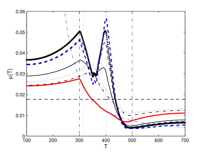
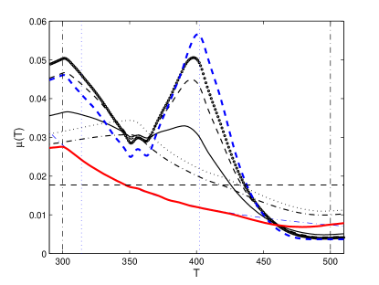
We solve minimization problem (9) using the Steepest Descent (SD), Conjugate Gradient (CG) and BFGS algorithms [26] and, unless indicated otherwise, using Sobolev gradients computed with $\ell=200.0$ which was found by trial–and–error to result in the fastest rate of convergence of iterations (14). The termination condition used was $\left|\frac{{\mathcal{J}}(\theta^{(n)})-{\mathcal{J}}(\theta^{(n-1)})}{{\mathcal{J}}(\theta^{(n-1)})}\right|<10^{-6}$. The behavior of the cost functional ${\mathcal{J}}(\theta^{(n)})$ as a function of the iteration count $n$ is shown in Figure 12a for all three minimization algorithms (SD, CG and BFGS). We note that in all cases a decrease over several orders of magnitude is observed in just a few iterations. Since the three descent methods tested reveal comparable performance, our subsequent computations will be based on the steepest descent method as the simplest one of the three. The effect of the different initial guesses $\mu_{0}$ on the decrease of the cost functional is illustrated in Figure 12b. Again, a substantial decrease of the cost functional corresponding to about 5–6 orders of magnitude is observed for all the initial guesses tested. Reconstructions $\hat{\mu}(T)$ of the constitutive relation obtained using the initial guess $\mu_{0}=\frac{C_{1}}{2}\left(e^{C_{2}/T_{\alpha}}+e^{C_{2}/T_{\beta}}\right)=0.0177$ and the optimization time windows with $t_{f}=\frac{1}{4},\frac{1}{2},1$ are shown in Figure 13. Comparing the accuracy of the reconstruction obtained for these different time windows, we can conclude that better results are achieved on shorter time windows $t_{f}=\frac{1}{4},\frac{1}{2}$. Given considerations of the computational time, hereafter we will therefore focus on the case with $t_{f}=\frac{1}{4}$. In Figure 14 we show the reconstructions $\hat{\mu}(T)$ of the constitutive relation obtained from different initial guesses already tested in Figure 12b such as constant values of $\mu_{0}$, $\mu_{0}(T)$ varying linearly with the temperature $T$ and $\mu_{0}$ given as a rescaling of the true relationship $\tilde{\mu}$. As expected, the best results are obtained in the cases where some prior information about the true material property is already encoded in the initial guess $\mu_{0}$, such as the slope, cf. Figure 14c, or the exponent, cf. Figure 14d. We may also conclude that, since all the reconstructions shown in Figures 13 and 14 are rather different, the iterations starting from different initial guesses converge in fact to different local minimizers. However, it should be emphasized that in all cases the reconstructions do capture the main qualitative features of the actual material property with differences becoming apparent only outside the measurement span interval ${\mathcal{M}}$. In order to make our tests more challenging, in the subsequent computations we will use the initial guess $\mu_{0}=\frac{1}{2}\left(\tilde{\mu}(T_{\alpha})+\tilde{\mu}(T_{\beta})\right)=0.0177$ (cf. Figure 13) which contains little prior information about the true material property.

In Figure 15 we show the results of the reconstruction performed with a larger identifiability region ${\mathcal{I}}=[250.0,700.0]={\mathcal{L}}$ which is done by adopting the corresponding values for temperature boundary conditions (2b), i.e., $T_{B}|_{\textrm{else}}=250$ and $T_{B}|_{\textrm{top}}=700$. We note that in this case the target interval for the reconstruction ${\mathcal{L}}$ has been chosen to coincide with identifiability interval ${\mathcal{I}}$. Fairly accurate reconstruction can be observed in this problem as well, and we emphasize that this is also the case for values of the temperature outside the identifiability interval studied in the previous case. This example demonstrates that accurate reconstruction on different intervals ${\mathcal{L}}$ can in fact be achieved by adjusting the identifiability region via a suitable choice of temperature boundary conditions (2b). This process can be interpreted as adjusting the conditions of the actual experiment used to obtain the measurements $\{\tilde{T}_{i}\}_{i=1}^{M}$.

Figure 12: (a) Decrease of the cost functional ${\mathcal{J}}(\theta^{(n)})$ with iterations $n$ using the Sobolev gradient $\boldsymbol{\nabla}^{H^{1}}_{\theta}{\mathcal{J}}$ defined in (31) and obtained with (solid line) steepest descent, (dash dotted line) conjugate gradient and (line with dots) BFGS methods with initial guess $\mu_{0}=0.0177$. (b) Decrease of the cost functional ${\mathcal{J}}(\theta^{(n)})$ with iterations $n$ for different initial guesses: (dots) $\mu_{0}=\tilde{\mu}(T_{\alpha})=0.0280$, (dash–dotted line) $\mu_{0}=\tilde{\mu}(T_{b})=0.0042$, (dashed line) $\mu_{0}(T)$ varying linearly between $\tilde{\mu}(T_{\alpha})$ and $\tilde{\mu}(T_{\beta})$, (thin solid line) $\mu_{0}=\frac{1}{2}\tilde{\mu}(T)$ and (thick solid line) $\mu_{0}=0.0177$.

Figure 13: Reconstruction $\hat{\mu}(T)$ of the material property obtained using the Sobolev gradients defined in (31) on (a,b,c) the interval ${\mathcal{L}}$ and (d) close–up view showing the interval outside the identifiability region ${\mathcal{I}}$ with the time window $[0,t_{f}]$, where (a) $t_{f}=\frac{1}{4}$ (b) $t_{f}=\frac{1}{2}$ and (c) $t_{f}=1$. The dash–dotted line represents the true material property (66), the thick solid, dashed and dash dotted lines are the reconstructions for (a,d) $t_{f}=\frac{1}{4}$, (b,d) $t_{f}=\frac{1}{2}$ and (c,d) $t_{f}=1$, respectively, whereas the dashed line represents the initial guess $\mu_{0}=0.0177$; the vertical dash–dotted and dotted lines represent, respectively, the boundaries of the identifiability interval ${\mathcal{I}}$ and the measurement span ${\mathcal{M}}$.

Figure 14: Reconstruction $\hat{\mu}(T)$ of the material property obtained using different initial guesses (a) $\mu_{0}=\tilde{\mu}(T_{\alpha})=0.0280$, (b) $\mu_{0}=\tilde{\mu}(T_{b})=0.0042$, (c) $\mu_{0}(T)$ varying linearly between $\tilde{\mu}(T_{\alpha})$ and $\tilde{\mu}(T_{\beta})$ and (d) $\mu_{0}=\frac{1}{2}\tilde{\mu}(T)$, and the Sobolev gradients defined in (31) on the interval ${\mathcal{L}}$. The dash–dotted line represents the true material property (66), the solid line is the reconstruction $\hat{\mu}(T)$, whereas the dashed line represents the initial guess $\mu_{0}$; the vertical dash–dotted and dotted lines represent, respectively, the boundaries of the identifiability interval ${\mathcal{I}}$ and the measurement span ${\mathcal{M}}$.

Figure 15: Reconstruction $\hat{\mu}(T)$ of the material property using an extended identifiability region ${\mathcal{I}}=[250.0,700.0]={\mathcal{L}}$ shown on (a) the interval $[100.0,700.0]$ and (b) magnification of this new identifiability region. The dash–dotted line represents the true material property (66), the solid line is the reconstruction $\hat{\mu}(T)$, whereas the dashed line represents the initial guess $\mu_{0}$; the vertical dash–dotted and dotted lines represent, respectively, the boundaries of the identifiability interval ${\mathcal{I}}_{0}=[300.0,500.0]$ used previously and the measurement span ${\mathcal{M}}$, while the dashed vertical lines show the boundaries of the new identifiability interval ${\mathcal{I}}$.

7.6 Reconstruction in the Presence of Noise

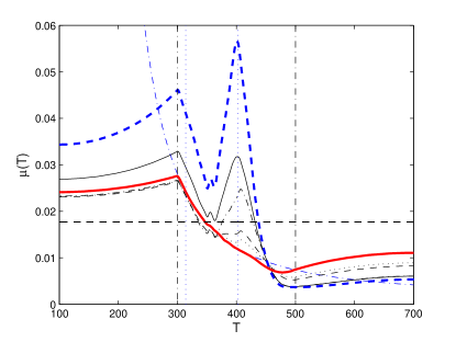
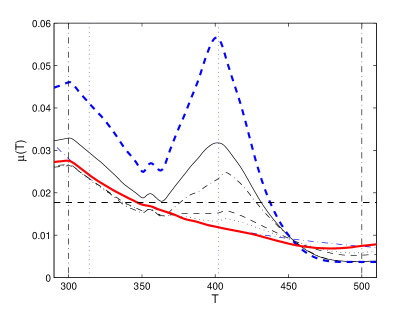
In this Section we first assess the effect of noise on the reconstruction without the Tikhonov regularization and then study the efficiency of the regularization techniques introduced in Section 5. In Figure 16a,b we revisit the case already presented in Figure 13a (reconstruction on the interval ${\mathcal{L}}=[100.0,700.0]$ with the identifiability region ${\mathcal{I}}=[300.0,500.0]$), now for measurements contaminated with 0.05%, 0.1%, 0.3%, 0.5% and 1.0% uniformly distributed noise and without Tikhonov regularization. To incorporate noise, say of $\eta\%$, into the measurements $\{\tilde{T}_{i}(t)\}_{i=1}^{M}$, we replace these measurements at every discrete time step $t_{j}\in[0,t_{f}]$ with a new set $\{\tilde{T}_{i}^{\eta}(t_{j})\}_{i=1}^{M}$, where the independent random variables $\tilde{T}_{i}^{\eta}(t_{j})$ have a uniform distribution with the mean $\tilde{T}_{i}(t_{j})$ and the standard deviation $\Delta\eta=\frac{1}{M}\sum_{i=1}^{M}\tilde{T}_{i}(t_{j})\cdot\frac{\eta}{100\%}$. Unless stated otherwise, in order to be able to directly compare reconstructions from noisy measurements with different noise levels, the same noise realization is used after rescaling to the standard deviation $\Delta\eta$. As expected, in Figure 16a,b we see that increasing the level of noise leads to oscillatory instabilities developing in the reconstructed constitutive relations $\hat{\mu}(T)$. We note that the reconstructions become poor already for relatively low noise levels, i.e., on the order of $1\%$. One reason for this seems to be the time-dependent nature of the problem in which independent noise is added to the measurements at every (discrete) time instant leading to accumulation of uncertainty. Indeed, such loss of information was not observed in the case of the steady problem studied in [7] where reliable reconstructions could be obtained with noise levels an order of magnitude larger than in the present investigation. In regard to the results shown in Figure 16a,b, we add that the pattern introduced by the noise in the reconstructions depends on the specific noise sample used (which was the same for all the reconstructions shown in the Figure). Reconstructions performed using different realizations of the noise produce distinct patterns in the reconstructed constitutive relations $\hat{\mu}(T)$. In our computational experiments we also observe that inclusion of noise in the measurements tends to replace the original minimizers with perturbed ones (this is evident from the uniform, with respect to $T$, convergence of the perturbed minimizers to the noise-free reconstructions as the noise level goes to zero in Figure 16a,b).

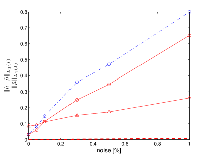
The effect of the Tikhonov regularization is studied in Figure 16c,d, where we illustrate the performance of the technique described in Section 5, cf. (33), on the reconstruction problem with 1.0% noise in the measurement data (i.e., the “extreme” case presented in Figures 16a,b). In terms of the (constant) reference function we take $\overline{\theta}=\sqrt{\mu_{0}-m_{\mu}}$, where $\mu_{0}=0.0177$. We note that by increasing the values of the regularization parameter $\lambda$ in (33) from 0 (no regularization) to 2500 we manage to eliminate the instabilities caused by the presence of noise in the measurements and obtain as a result smoother constitutive relations, cf. Figure 16c,d. We add that, while after introducing the Tikhonov regularization the reconstructed solutions converge in fact to different local minimizers (in comparison with the reconstructions without noise), this does not prevent the reconstructions from capturing the main qualitative features of the actual material property. Systematic methods for determining the optimal values of regularization parameters are discussed for instance in [30]. Finally, in Figure 17 we present the relative reconstruction errors $\|\hat{\mu}-\tilde{\mu}\|_{L_{1}({\mathcal{I}})}\,/\,\|\tilde{\mu}\|_{L_{1}({\mathcal{I}})}$ obtained using the approach described earlier in Section 5 for data with different noise levels and averaged over 10 different noise samples. From Figure 17 we conclude that larger values of the regularization parameter $\lambda$ are required for more noisy measurements. We close this Section by concluding, in agreement with our earlier results reported in [7], that Tikhonov regularization performs as expected in problems with noise present in the measurement data.

Figure 16: (a,b) Reconstruction $\hat{\mu}(T)$ of the material property obtained in the presence of different noise levels in the measurement data: (thick solid line) no noise, (dotted line) 0.05%, (dashed line) 0.1%, (dash–dotted line) 0.3%, (thin solid line) 0.5%, and (thick dashed line) 1.0% on (a) the interval ${\mathcal{L}}$ and (b) close–up view showing the identifiability interval ${\mathcal{I}}$. (c,d) Effect of Tikhonov regularization on the reconstruction from the measurement data with 1.0% noise using regularization term (33) on (c) the interval ${\mathcal{L}}$ and (d) close–up view showing the identifiability interval ${\mathcal{I}}$. In both figures (c,d) the following values of the regularization parameter were used: (thick dashed line) $\lambda=0$, (circles) $\lambda=2.5$, (dashed line) $\lambda=6.25$, (thin solid line) $\lambda=25.0$, (dash–dotted line) $\lambda=250.0$, and (dots) $\lambda=2500.0$. For all figures the horizontal dashed line represents the initial guess $\mu_{0}=0.0177$; the vertical dash–dotted and dotted lines represent, respectively, the boundaries of the identifiability interval ${\mathcal{I}}$ and the measurement span ${\mathcal{M}}$.

Figure 17: Relative $L_{1}$ reconstruction errors $\|\hat{\mu}-\tilde{\mu}\|_{L_{1}({\mathcal{I}})}\,/\,\|\tilde{\mu}\|_{L_{1}({\mathcal{I}})}$ obtained in the presence of noise with the amplitude indicated and averaged over 10 samples: (dash–dotted line) reconstruction with Sobolev gradients and without Tikhonov regularization, and (solid line) reconstruction with $\dot{H}^{1}$ Tikhonov regularization term (33) [(circles) $\lambda=2.5$, (triangles) $\lambda=250.0$]. The thick dashed line represents the “error” in the exact material property (66) obtained by adding noise to $T$ and averaging over time steps.

8 Conclusions and Summary

We developed an optimization–based approach to the problem of reconstructing temperature–dependent material properties in complex thermo–fluid systems. As a model problem we considered two–dimensional unsteady flows in a lid–driven cavity involving also heat transfer. A key element of this approach is the gradient of the cost functional which is computed based on a suitably–defined adjoint system, and is shown to have mathematical structure different than in most problems involving adjoint–based PDE optimization. We discussed three different numerical approaches to evaluation of these cost functional gradients which are given in terms of integrals defined on the level sets of the temperature field. As compared to earlier work on the numerical approximation of such expressions [8, 9, 10, 11, 12, 15, 16, 13, 14], we also addressed at length the question of the discretization of the solution space which is specific to our reconstruction problem. Evidence is shown for the superior performance with respect to the discretizations of the physical and the solution space, as well as the computational time, of a new approach to evaluation of gradients which is proposed in this study.

The reconstruction results obtained demonstrate good performance of the algorithm, in particular, it is shown that by suitably adjusting the boundary conditions in the governing system we can extend the identifiability region. There are two comments we wish to make concerning these results. As regards the data shown in Figure 13, it might appear somewhat surprising that reconstructions on longer time windows (which use more information from the measurements) do not necessarily lead to better results. A probable reason is that such reconstruction problems defined on longer time windows tend to be harder to solve numerically, hence the solutions found may not be global minimizers (or even “good” local ones). Another comment we have concerns the relatively modest noise levels for which stable reconstructions could be obtained in Section 7.6. We note that inclusion of even a small amount of noise could alter the nature of the reconstructed constitutive relations. On the other hand, we also remark that reconstructions performed based on a steady-state problem and reported in [7] did allow for significantly higher noise levels. We therefore conjecture that the sensitivity to noise in the present problem is related to its time-dependent character, as here the effect of instantaneously small noise levels may be compounded by its continuous accumulation over the entire time window. Since the flow problem studied here was admittedly very simple, this issue may certainly limit the applicability of the proposed method to problems characterized by higher Reynolds numbers and therefore merits a more thorough study in the future (this is not the question of the numerical resolution alone, but rather of the interplay between this resolution and the complexity of the underlying optimization problem). Experience with other data assimilation problems may suggest that acquiring the measurements less frequently in time may actually help mitigate this effect.

The approach developed in the present study was recently successfully applied to the problem of system identification involving a dynamical system in the phase-space representation. More precisely, in [40] we used this method to reconstruct an invariant manifold in a realistic reduced-order model of a hydrodynamic instability. Our future work will involve extensions of the present approach to more complicated problems involving systems of coupled PDEs depending on time and defined on domains in three dimensions. In the context of such systems an interesting issue is the reconstruction of anisotropic constitutive relations. A more challenging problem is related to reconstruction of constitutive relations in systems involving phase changes. In addition to the governing PDE in the form of a free–boundary problem, one would also have to deal with constitutive relations with distinct functional forms in each of the phases. Interesting questions also arise in the reconstruction of material properties defined on the interfaces between different phases, such as for example the temperature–dependent surface tension coefficient playing an important role in Marangoni flows. In the study of such more complicated problems close attention will need to be paid to the question of ensuring consistency of the reconstructed constitutive relation with the second principle of thermodynamics, which can be done by including a form of the Clausius–Duhem inequality [20] in the optimization formulation. In such more general problems it is not obvious whether this additional constraint can be eliminated by introducing a slack–variable formulation similar to the one used in this study, and one may have to perform numerical optimization in the presence of inequality constraints. These questions are left for future research.

References

- [1] O. Volkov, B. Protas, W. Liao and D. Glander, “Adjoint–Based Optimization of Thermo–Fluid Phenomena in Welding Processes”, Journal of Engineering Mathematics 65, 201–220, (2009).
- [2] V. Isakov, Inverse Problems for Partial Differential Equations, Springer, (2006).
- [3] A. Tarantola, Inverse Problem Theory and Methods for Model Parameter Estimation, SIAM (2005).
- [4] M. Z. Nashed and O. Scherzer, Inverse Problems, Image Analysis, and Medical Imaging, AMS (2002).
- [5] J. Gottlieb and P. DuChateau, Parameter Identification and Inverse Problems in Hydrology, Geology, and Ecology, Kluwer Academic Publishers (1996)
- [6] G. Chavent and P. Lemonnier, “Identification de la Non–Linearité D’Une Équation Parabolique Quasilineaire”, Applied Mathematics and Optimization 1, 121–162, (1974).
- [7] V. Bukshtynov, O. Volkov, B. Protas, “On Optimal Reconstruction of Constitutive Relations”, Physica D 240, 1228–1244, (2011).
- [8] B. Engquist, A.-K. Tornberg and R. Tsai, “Discretization of Dirac Delta Functions in Level Set Methods”, Journal of Computational Physics 207, 28–51, (2004).
- [9] S. Zahedi, A.-K. Tornberg, “Delta Functions Approximations in Level Set Methods by Distance Function Extension”, Journal of Computational Physics 229, 2199–2219, (2010).
- [10] A. Mayo, “The Fast Solution of Poisson’s and the Biharmonic Equations on Irregular Regions”, SIAM Journal of Numerical Analysis 21, 285–299, (1984).
- [11] P. Smereka, “The Numerical Approximation of a Delta Function with Application to Level Set Methods”, Journal of Computational Physics 211, 77–90, (2006).
- [12] J. T. Beale, “A Proof That a Discrete Delta Function is Second-Order Accurate”, Journal of Computational Physics 227, 2195–2197, (2008).
- [13] J. D. Towers, “Discretizing Delta Functions via Finite Differences and Gradient Normalization”, Journal of Computational Physics 228, 3816–3836, (2009).
- [14] J. D. Towers, “Two Methods for Discretizing a Delta Function Supported on a Level Set”, Journal of Computational Physics 220, 915–931, (2007).
- [15] C. Min, F. Gibou, “Geometric Integration over Irregular Domains with Application to Level–Set Methods”, Journal of Computational Physics 226, 1432–1443, (2007).
- [16] C. Min, F. Gibou, “Robust Second–Order Accurate Discretizations of the Multi-Dimensional Heaviside and Dirac Delta Functions”, Journal of Computational Physics 227, 9686–9695, (2008).
- [17] W. Muschik, “Aspects of Non–Equilibrium Thermodynamics”, World Scientific, (1989).
- [18] B. D. Coleman and W. Noll, “The Thermodynamics of Elastic Materials with Heat Conduction and Viscosity”, Arch. Rat. Mech. Anal 13, 167–178, (1963).
- [19] I.-S. Liu, “Method of Lagrange Multipliers for Exploitation of the Entropy Principle”, Arch. Rat. Mech. Anal 46, 131–148, (1972).
- [20] V. Triano, Ch. Papenfuss, V. A. Cimmelli, and W. Muschik, “Exploitation of the Second Law: Coleman–Noll and Liu Procedure in Comparison”, J. Non–Equilib. Thermodyn. 33, 47–60, (2008).
- [21] Ph. Kügler, “Identification of a Temperature Dependent Heat Conductivity from Single Boundary Measurements”, SIAM J. Numer. Anal. 41, 1543–1563, (2003).
- [22] A. Ruszczyński, Nonlinear Optimization, Princeton University Press (2006).
- [23] C. R. Vogel, Computational Methods for Inverse Problems, SIAM (2002).
- [24] S. Boyd and L. Vandenberghe, Convex Optimization, Cambridge University Press, (2004).
- [25] D. Luenberger, Optimization by Vector Space Methods, John Wiley and Sons (1969).
- [26] J. Nocedal and S. Wright, Numerical Optimization, Springer (2002).
- [27] M. S. Berger, Nonlinearity and Functional Analysis, Academic Press (1977).
- [28] M. D. Gunzburger, Perspectives in Flow Control and Optimization, SIAM (2003).
- [29] B. Protas, T. Bewley and G. Hagen, “A Comprehensive Framework for the Regularization of Adjoint Analysis in Multiscale PDE Systems”, Journal of Computational Physics 195, 49–89, (2004).
- [30] H. Engl, M. Hanke and A. Neubauer, Regularization of Inverse Problems, Kluwer (1996).
-
[31]
V. Bukshtynov, Computational Methods for the