Phase Diagram and Approximate Message Passing for Blind Calibration and Dictionary Learning

Abstract

We consider dictionary learning and blind calibration for signals and matrices created from a random ensemble. We study the mean-squared error in the limit of large signal dimension using the replica method and unveil the appearance of phase transitions delimiting impossible, possible-but-hard and possible inference regions. We also introduce an approximate message passing algorithm that asymptotically matches the theoretical performance, and show through numerical tests that it performs very well, for the calibration problem, for tractable system sizes.

I Introduction

Matrix decomposition $Y=FX$, where $Y$ is known and one seeks $F$ and $X$, with requirements (e.g. sparsity, probability distribution of elements etc.) on the properties of $X$ and $F$, is a generic problem that appears in many applications [1]. Theoretical limits on when matrix decompositions is possible and tractable are still very poorly understood. In this work we make a step towards this understanding by determining the limits of matrix decomposition when $Y$ is created using randomly generated matrices $F$ and $X$.

Consider a set of $P$ $K$-sparse $N$-dimensional vectors (“signals”), with iid components created from the distribution (denoting $\rho=K/N$)

$$P(x^{0}_{il})\!=\!(1-\rho)\delta(x^{0}_{il})+\rho{\phi}(x^{0}_{il}),$$ (1)

where $i\!=\!1,\ldots,N$, $l\!=\!1,\ldots,P$. For each of the vectors we perform $M$ linear measurements, summarized by a $M\!\times\!N$ measurement matrix with iid elements $\mathcal{F}^{0}_{\mu i}=F^{0}_{\mu i}/\sqrt{N}$ (this rescaling ensures that the measurements are of $O(1)$) where the $F^{0}_{\mu i}$ are generated from a probability distribution $\phi_{F}(F^{0}_{\mu i})$ (in the numerical examples we will always consider a Gaussian distribution of zero mean and unit variance). We have only access to the (noisy) results of these measures, that is, to the $P$ vectors ${y}_{l}$ such that

$$y_{\mu l\!}=\!\sum_{i}\mathcal{F}_{\mu i}^{0}x_{il}^{0}+\xi_{\mu l}\,,$$ (2)

where $\xi_{\mu l}$ is a Gaussian additive noise with variance $\Delta$.

Is it possible to find both the vectors $x^{0}$ and the matrix (dictionary) $F^{0}$ (up to a permutation of $N\!$ elements and their signs)? This is the dictionary learning problem. A related situation is when one knows at least a noisy version of the matrix $F^{0}$, defined by $F^{\prime}=(F^{0}+\sqrt{\eta}W)/\sqrt{1+\eta}$ where $W$ is a random matrix with the same statistics as $F^{0}$. $P(F^{0}|F^{\prime})$ then reads, for each matrix element

$$P(F^{0}_{\mu i}|F^{\prime}_{\mu i})={\cal N}(\frac{F^{\prime}_{\mu i}}{\sqrt{1+\eta}},\frac{\eta}{1+\eta})\,.$$ (3)

Recovering $F^{0}$ and $x^{0}$, knowing this time $F^{\prime}$ and the $P$ vectors $y_{l}$ is a problem that we shall refer to as blind calibration. It becomes equivalent to dictionary learning when $\eta\to\infty$.

Our goal here is to analyse optimal Bayes inference (that provides the MMSE (minimal MSE)) where the signal $x_{il}^{0}$ and the dictionary $F^{0}_{\mu i}$ are estimated from the marginals of the posterior probability

$$P(x_{il},F_{\mu i}|y_{\mu l},F^{\prime}_{\mu i})=\frac{1}{Z}\prod_{\mu i}P(F_{\mu i}|F^{\prime}_{\mu i})$$

$$\prod_{il}\!P(x_{il})\prod_{\mu l}\!\!\left[\frac{1}{\sqrt{2\pi\Delta}}e^{-\frac{(y_{\mu l}-\sum_{i}F_{\mu i}x_{il}/\sqrt{N})^{2}}{2\Delta}}\!\right]\,.$$ (4)

I-A Related works

There are several algorithm suggested and tested for dictionary learning, see e.g. [2, 3, 4, 5]. The algorithm we derive in this paper is closely related but different to the bilinear AMP proposed by [6] as explained in Sec. III.

The question of how many samples $P$ are necessary for the dictionary to be identifiable has a straightforward lower bound $MP>N(M+P\rho)$, otherwise there is more unknown variables than measurements and hence exact recovery is clearly impossible. Several works analyzed what is a sufficient number of samples for exact recovery. While early rigorous results were able to show learnability from only exponential many samples [7], more recent analysis of convex relaxation based approaches shows that $O(N\log{N})$ samples are needed for $\alpha=1$ [8] and polynomially many for $\alpha<1$ [9]. Another study of sample complexity for dictionary learning for $\alpha<1$ establishes a $O(N\log{N})$ bound for the number of samples [10]. A very recent non-rigorous work suggested that $P\!=\!O(N)$ samples should be sufficient to identify the dictionary [11]. That work was based on the replica analysis of the problem, but did not analyze the Bayes-optimal approach.

Several works also considered blind calibration, where only a uncertain version of the matrix $F$ is known, on the other hand one has the access to many signals and their measurements such that calibration of the matrix $F$ is possible, see e.g. [12] and reference therein. Cases when both the signal and the dictionary are sparse are also considered in the literature, e.g. [13], and our theory can be applied to these as well.

I-B Main results

The present paper has three main results. First, using the replica method [14] we estimate the Bayes optimal MMSE in the limit of large signals $N\to\infty$. In particular, we define $\alpha\!=\!M/N$, $\pi\!=\!P/N$ and show that for the noiseless case, $\Delta=0$, exact reconstruction is possible if $\pi\!>\!\pi^{*}\!=\!{\alpha}/{(\alpha-\rho)}$ and $\alpha>\rho$. In this regime, it is thus possible to recover the matrix and the signal exactly if one can compute the marginals of the posterior probability distribution (4). This result is striking, all the more because it is independent of $\eta$.

Computing the marginals of the posterior probability distribution is an extremely hard problem, all the more when there is a phase transition in the problem. We determine the value $\pi^{s}(\eta)$ (the spinodal transition) below which iterative sampling (using for instance Monte Carlo Markov chains or message passing) is believed to be intractable in polynomial time.

Finally, we introduce an AMP-like message passing algorithm designed to perform such sampling, and show that it performs very well for the calibration problem. However, at the moderate size we are able to study numerically, finite-size deviation from the asymptotic behavior become large as $\eta$ grows and prevents our algorithm to function nicely in the dictionary learning limit. However, we believe that this still sets a very promising stage for new algorithmic development for dictionary learning.

II Asymptotic analysis with the replica method

II-A Replica analysis for matrix decomposition

Figure 1: Phase diagram for $\alpha\!=\!0.5$ and $\Delta\!=\!0$. For both blind calibration and dictionary learning, exact learning is possible by the Bayes optimal approach above the full red line $\pi^{*}=\frac{\alpha}{\alpha-\rho}$. However, such a sampling procedures will not be tractable below the spinodal transition $\pi^{s}(\eta)$ shown here in dotted line for dictionary learning ($\eta\!=\!\infty$) and blind calibration.

Figure 2: MMSE $D$ (for the matrix $F$) and $E$ (for the signal ${x}$) corresponding to $\rho=0.2$, $\alpha=0.5$, $\Delta=0$, for three values of $\eta$. The MMSE jumps abruptly from a finite value to zero at $\pi^{*}$. However, sampling should remain intractable until the spinodal transition arises at a larger value $\pi^{s}(\eta)$ and we denote the corresponding MSE in dotted line. The figure remains qualitatively the same for small value of the additive noise $\Delta>0$, where the MMSE at large $\pi$ is not zero but rather $O(\Delta)$. If $\Delta$ is large enough, however, the sharp transition disappears and the MMSE is continuous (see e.g. Fig. 4).

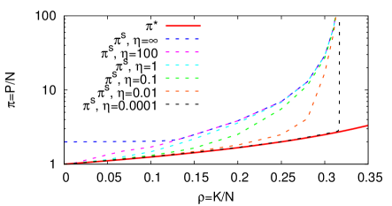
The MMSE obtained from the Bayes-optimal approach can be computed exactly in the limit of large $N$ via the replica method. Although this method is in general non-rigorous, it is sometimes possibles to prove that the results derived from it are exact., We shall leave out details of the derivation and refer instead to [15, 16] for a very similar computation in the case of compressed sensing. We estimate the Bayes optimal MMSE by computing the marginals of the matrix and signals elements. Our computation is also very similar to the one of [11], who however did not analyze the Bayes optimal MMSE.

We now compute $\Phi={\mathbb{E}}_{F^{0},F^{\prime},x^{0}}(\log{Z(F^{0},F^{\prime},x^{0})})/NP$, where $Z$, the so-called partition sum (or evidence), is the normalization in eq. (4) for a given instance of the problem. In order to do so we compute ${\mathbb{E}}_{F^{0},F^{\prime},x^{0}}(Z^{n})$ and then use the replica trick $\log{Z}=\lim_{n\to 0}(Z^{n}-1)/n$. We use the replica symmetric ansatz which is correct for inference problems with prior distributions corresponding to the generative process. The final result is that in the large signal limit, $N\to\infty$, the MMSE $D$ (on the matrix) and $E$ (on the signals) are given by

$${\rm MMSE}(\alpha,\pi,\rho,\Delta,\eta)=\arg\!\max_{E,D}\Phi(E,D)\,,$$ (5)

where the so-called “potential” is given by

$$\!\!\!\!\!\!\!\!\!\!\!\!\!\Phi(\!E\!,\!D\!)\!\!=\!\!-\frac{\alpha}{2}\log{(\Delta\!+\!E\!+\!D(\rho-E))}\!\!-\!\!\frac{\alpha(\Delta+\rho)}{\Delta+E+D(\rho-E)}$$

$$+ \!\!\!\!\frac{\alpha}{2}+\!\!\left[\int{\cal D}z\log{\left\{\left[e^{-\frac{\hat{m}_{x}}{2}x^{2}+\hat{m}_{x}xx^{0}+z\sqrt{\hat{m}_{x}}x}\right]_{P(x)}\right\}}\right]_{P(x^{0})}$$

$$+ \!\!\!\!\!\!\frac{\alpha}{\pi}\!\!\left[\int{\cal D}z\!\log{\left[e^{-\frac{\hat{m}_{F}F^{2}}{2}+\hat{m}_{F}FF^{0}+z\sqrt{\hat{m}_{F}}F}\right]_{P(F|F^{\prime})}}\right]_{\!P(F^{0}\!,F^{\prime})}\,.$$

Here $[f(u)]_{Q(u)}$ denotes an average of a function $f$ of the random variable $u$ with distribution $Q(u)$, ${\cal D}z$ a Gaussian measure with zero mean and unit variance. The probability distributions $P(x)$, and $P(F|F^{\prime})$ are the single-element distributions introduced in eqs. (1) and (3). Finally we denoted

$$\hat{m}_{x}\!=\!\frac{\alpha(1-D)}{\Delta+E+\rho D-ED},~{}~{}~{}\hat{m}_{F}\!=\!\frac{\pi(\rho-E)}{\Delta+E+\rho D-ED}\,.$$ (6)

Note that the present expression for the potential is very general and can be used to study many similar problems, such as matrix completion, or sparse matrix decomposition, by changing the distribution of the matrix and of the signal.

II-B Gaussian matrix and Gauss-Bernoulli signal

When the matrix elements $F^{0}_{\mu i}$ are generated from a Gaussian with zero mean and unit variance, and $x^{0}_{il}$ from Gauss-Bernoulli distribution, the potential simplifies to

$$\!\!\!\!\!\!\!\!\!\!\!\!\!\Phi(E,D)\!\!=\!\!-\frac{\alpha}{2}\!\log{(\Delta\!+\!E\!+\!D(\rho-E))}\!\!-\!\!\frac{\alpha(\Delta+\rho)}{\Delta\!+\!E\!+\!D(\rho-E)}$$ (7)

$$+ \!\!\frac{\alpha}{2}+(1-\rho)\int{\cal D}z\,\log{\left(1-\rho+\frac{\rho}{\sqrt{\hat{m}_{x}+1}}e^{\frac{z^{2}\hat{m}_{x}}{2(\hat{m}_{x}+1)}}\right)}$$

$$+ \!\!\!\rho\!\int{\!\!\cal D}z\log{\!\left(\!1\!-\!\rho\!+\!\frac{\rho}{\sqrt{\hat{m}_{x}\!+\!1}}e^{\frac{z^{2}\hat{m}_{x}}{2}}\!\right)}+\frac{\alpha}{2\pi}\!\hat{m}_{F}$$

$$- \frac{\alpha}{2\pi}\log{\left(1+\frac{\eta\hat{m}_{F}}{1+\eta}\right)}\,.$$

The Bayes-optimal MMSE is obtained by maximizing $\Phi(E,D)$. Analyzing the above expression in the zero-noise limit ($\Delta=0$) allows to demonstrate our first main result: in both the blind calibration and dictionary learning problems, the global maximum is given by $D\!=\!E\!=\!0$, with $\Phi\to\infty$, as long as $\alpha\!>\!\rho$ and $\pi\!>\!\pi^{*}\!=\!{\alpha}/{(\alpha-\rho)}$. Hence for $\pi\!>\!\pi^{*}$ it is possible to learn the matrix and the signal exactly from the measurements. This result is striking since it is independent of $\eta$ as long as $\eta>0$; and coincides with the simple counting lower bound. When $\eta\to 0$, more precisely when $\eta\ll\Delta$, then the compressed sensing phase transition —that goes to $\alpha=\rho$ when $\Delta\to 0$— is recovered independently of $\pi$.

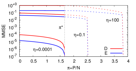
Bayes-optimal learning, however, requires exact sampling from the measure (4), and this remains an extremely hard computational problem. In this regard, another important transition (the “spinodal”), that can be studied from the form of the potential function $\Phi(E,D)$, is the appearance of a high-MSE local maxima. This phenomenon marks the downfall of many sampling strategy, such as Gibbs sampling or message-passing strategy (that performs a steepest ascent in the $\Phi(E,D)$ function). We determine the value $\pi^{s}(\eta)$ (the so-called “spinodal” transition) above which $\Phi(E,D)$ does not have the spurious secondary maxima. As shown in Fig. 1 and Fig. 2, it depends strongly on the value $\eta$. In fact, when $\eta\to 0$, we recover again the compressed sensing limit we have obtained in [16]. Figs. 2 and 4 depict the values of MMSE for the signal $E$ and the matrix $D$ reached for large systems $N\to\infty$ by the Bayes optimal sampling and by local sampling strategies that reach $D=E=0$ discontinuously at $\pi^{s}$.

The behavior with finite noise $\Delta<\eta$ is also interesting and we observe a phenomenology similar to that described in [16] in the case of compressed sensing. Because of a two-maxima shape of the function $\Phi(E,D)$ for moderate $\Delta$, the MMSE displays a sharp transition separating a region of parameters with a small MMSE, comparable to $\Delta$, from a region with a larger $O(\eta)$ MMSE. For larger value of $\Delta$ we do not see any abrupt transition, and the MMSE continuously decays with $\pi$ (see e.g. Fig. 4).

To conclude, there exist three regions in the phase diagram, corresponding to impossible (below $\pi^{*}$), intractable (below $\pi^{s}$), and perhaps-tractable learning. We will now study algorithmically the later one.

III Message-passing algorithm

To make the Bayes optimal sampling tractable we have to resort to approximations. In compressed sensing, the Bayesian approach combined with a belief propagation (BP) reconstruction algorithm leads to the so-called approximate message passing (AMP) algorithm. It was first derived in [17] for the minimization of $\ell_{1}$, and subsequently generalized in [18, 19]. We shall now adapt this strategy to the present case.

III-A From BP to AMP

Figure 3: Factor graph used for the belief propagation inference, here drawn using $N=3$, $P=2$ and $M=2$. The factor nodes ensure (in probability) the condition $y_{\mu l\!}=\!\sum_{i}\mathcal{F}_{\mu i}x_{il}+\xi_{\mu l}$.

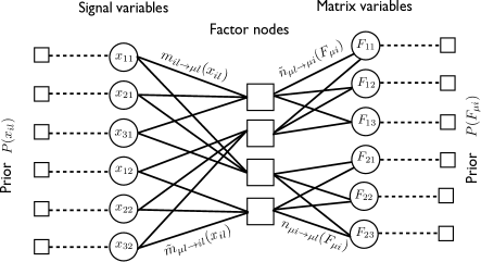
The factor graph corresponding to the posterior probability (4) is depicted in Fig. 3. The canonical BP iterative equations are written for messages $m,n,\hat{m},\hat{n}$ and read

$$m_{il\to\mu l}(x_{il}) \propto P(x_{il})\prod_{\nu\neq\mu}^{M}\hat{m}_{\nu l\to il}(x_{il})\,,$$ (8)

$$n_{\mu i\to\mu l}(F_{\mu i}) \propto P(F_{\mu i}|F^{\prime}_{\mu i})\prod_{n\neq l}^{P}\hat{n}_{\mu n\to\mu i}(F_{\mu i})\,,$$ (9)

$$\hat{m}_{\mu l\to il}(x_{il}) \propto \int\prod_{j\neq i}dx_{jl}dF_{\mu k}e^{-\frac{(y_{\mu l}-\sum_{i}F_{\mu i}x_{il}/\sqrt{N})^{2}}{2\Delta}}$$ (10)

$$\prod_{k}n_{\mu k\to\mu l}(F_{\mu k})\prod_{j\neq i}m_{jl\to\mu l}(x_{jl})\,,$$

$$\hat{n}_{\mu l\to\mu i}(F_{\mu i}) \propto \int dx_{jl}\prod_{k\neq i}dF_{\mu k}e^{-\frac{(y_{\mu l}-\sum_{i}F_{\mu i}x_{il}/\sqrt{N})^{2}}{2\Delta}}$$ (11)

$$\prod_{k\neq i}n_{\mu k\to\mu l}(F_{\mu k})\prod_{j}m_{jl\to\mu l}(x_{jl})\,.$$

A major simplification of these iterative equations arises when one uses the central limit theorem and realizes that only the two first moments of the above distributions are important for the leading contribution when $N\to\infty$. This ”Gaussian” approximation is at the basis of approximate message passing as used in compressed sensing. The next step of the derivation again neglects $O(1/N)$ terms and allows to reduce the number of messages to be iterated from $O(N^{4})$ to $O(N^{2})$. This leads to a TAP-like set of equations [20]. Finally if the matrix $F^{0}$ and signal $x^{0}$ have known distribution of elements this further simplifies the algorithm. A full derivation will be given elsewhere and we instead refer the reader to the re-derivation of AMP in [16] where we followed essentially the very same steps.

The final form of our algorithm for blind calibration and dictionary learning follows. We denote the mean and variance of the BP estimates of marginals over $x_{il}$ as $a_{il}$ and $c_{il}$, and those over $\mathcal{F}_{\mu i}$ as $r_{\mu i}$ and $s_{\mu l}$. We define several auxiliary values (all of them are of order $O(1)$):

$$\overline{a^{2}} = \frac{1}{NP}\sum_{jl}a^{2}_{jl},~{}~{}\overline{c}=\frac{1}{NP}\sum_{jl}c_{jl}\,,$$

$$\overline{r^{2}} = \frac{1}{M}\sum_{\nu j}r^{2}_{\nu j},~{}~{}\overline{s}=\frac{1}{M}\sum_{\nu j}c_{\nu j}\,,$$

$$\overline{(y-\omega)^{2}} = \frac{1}{MP}\sum_{\nu l}(y_{\nu l}-\omega_{\nu l})^{2}\,.$$

Then our AMP algorithm reads

$$\omega_{\nu l}^{t+1} = \sum_{j}r_{\nu j}a_{jl}^{t}-\frac{y_{\nu l}-\omega^{t}_{\nu l}}{\overline{(y-\omega)^{2}}^{t}}(\overline{c}^{t}\overline{r^{2}}^{t}+\overline{a^{2}}^{t}\overline{s}^{t})\,\!\!,$$ (12)

$$(\Sigma_{R}^{t+1})^{2} = \left[\alpha\frac{\overline{r^{2}}^{t}}{\overline{(y-\omega)^{2}}^{t+1}}\right]^{-1}\,,$$ (13)

$$(\Sigma_{S}^{t+1})^{2} = \left[\pi\frac{\overline{a^{2}}^{t}}{\overline{(y-\omega)^{2}}^{t+1}}\right]^{-1}\,,$$ (14)

$$R_{il}^{t+1} = a_{il}^{t}-a_{il}^{t}\frac{\overline{s}^{t}}{\overline{r^{2}}^{t}}+\frac{\sum_{\nu}(y_{\nu l}-\omega_{\nu l}^{t+1})r_{\nu i}^{t}}{\alpha\overline{r^{2}}^{t}}\,,$$ (15)

$$S_{\nu i}^{t+1} = r_{\nu i}^{t}-r_{\nu i}^{t}\frac{\overline{c}^{t}}{\overline{a^{2}}^{t}}+\frac{\sum_{l}(y_{\nu l}-\omega_{\nu l}^{t+1})a_{il}^{t}}{N\pi\overline{a^{2}}^{t}}\,,$$ (16)

$$a^{t+1}_{il} = f_{a}\left((\Sigma_{R}^{t+1})^{2},R^{t+1}_{il}\right),$$ (17)

$$v^{t+1}_{il} = f_{c}\left((\Sigma_{R}^{t+1})^{2},R^{t+1}_{il}\right)\,,$$ (18)

$$r^{t+1}_{\mu i} = f_{r}\left((\Sigma_{S}^{t+1})^{2},S^{t+1}_{\mu i}\right),$$ (19)

$$s^{t+1}_{\mu i} = f_{s}\left((\Sigma_{S}^{t+1})^{2},S^{t+1}_{\mu i}\right)\,.$$ (20)

where only the following functions are prior-dependent:

$$f_{a}(\Sigma^{2},T) = \frac{\rho\,e^{-\frac{T^{2}}{2(\Sigma^{2}+1)}}\frac{\Sigma}{(\Sigma^{2}+1)^{\frac{3}{2}}}(\Sigma^{2}+T)}{(1-\rho)e^{-\frac{T^{2}}{2\Sigma^{2}}}+\rho\frac{\Sigma}{\sqrt{\Sigma^{2}+1}}e^{-\frac{T^{2}}{2(\Sigma^{2}+1)}}}\,,$$ (21)

$$f_{c}(\Sigma^{2},T) = \Sigma^{2}\frac{{\rm d}}{{\rm d}T}f_{a}(\Sigma^{2},T)\,,$$ (22)

$$f_{r}(\Sigma^{2},T) = \frac{T+\Sigma^{2}F^{\prime}_{\mu i}\frac{\sqrt{1+\eta}}{\sqrt{N}\eta}}{(1+\frac{1}{\eta})\Sigma^{2}+1}\,,$$ (23)

$$f_{s}(\Sigma^{2},T) = \frac{1}{N}\frac{\Sigma^{2}}{(1+\frac{1}{\eta})\Sigma^{2}+1}\,.$$ (24)

Initial conditions are set so that the marginals correspond to the means and variances of the prior, and $\omega_{\mu l}=y_{\mu l}$. One iteration of the algorithm takes $O(N^{3})$ steps. In practice, we also damp the expressions (17,18,19,20) to ensure convergence. If the matrix elements are not learned, this algorithm reduces to the AMP for matrix uncertainty from [21], and is asymptotically equivalent to the MU-AMP of [22]. The bilinear AMP suggested in [6] for matrix decomposition consists of fixing a current value of $F$ and its uncertainty, running MU-AMP, then fixing a current values of $x$ and its variances, running MU-AMP, and repeating. Whereas the difference in performances between the present algorithm and the one of [6] is yet to be studied, it is not clear if the later implements asymptotically the Bayes optimal inference, and neither if the state evolution (next paragraph) applies to it.

III-B State evolution

The AMP approach is amenable to asymptotic ($N\to\infty$) analysis using a method known as “cavity method” in statistical physics [14], or “state evolution” in compressed sensing [17]. Given the parameters $\rho$, $\alpha$,$\pi$ $\eta$, $\Delta$, the MSE given by our approach follows, in the infinite size limit:

$$E^{t+1} = (1-\rho)\int{\cal D}zf_{c}(\hat{m}_{x},z\sqrt{\hat{m}_{x}})$$ (25)

$$+ \rho\int{\cal D}zf_{c}(\hat{m}_{x},z\sqrt{\hat{m}^{2}_{x}+\hat{m}_{x}})\,,$$

$$D^{t+1} = \frac{1}{\hat{m}_{F}+\frac{1+\eta}{\eta}}\,,$$ (26)

where $\hat{m}_{F}^{t}$ and $\hat{m}_{x}^{t}$ follow from eq. (6), with $E^{t},D^{t}$ on the right hand side, $E^{t=0}=\rho$, $D^{t=0}=1$, ${\cal D}z$ is a Gaussian integral, and $f_{c}$ is defined by eq. (22).

From eqs. (25,26), one can show that the evolution of the algorithm is equivalent to a steepest ascent of the potential $\phi(E,D)$ obtained in eq. (7). This explains the peculiar meaning of the spinodal transition arising at $\pi^{s}$ and shows that for $\pi>\pi^{s}$ our algorithm should approximates correctly the Bayes optimal inference for matrix decomposition for large systems, $N\to\infty$, as AMP does for compressed sensing. Note that in the later case, the state evolution approach has been proveen rigorously [23] and would be interesting to see if this could be generalize to the present, arguably more complex, case.

III-C Numerical tests

Figure 4: Comparison of the performance of the AMP algorithm with the MMSE $D$ (for the matrix) and $E$ (for the signal, fewer points are shown for visibility) for different system sizes $N$. Top: A case with continuous decay of the MMSE for $\Delta=10^{-8}$, $\eta=10^{-4}$, $\alpha=0.3$, $\rho=0.1$. The initial error on the matrix is about $1\%$. Bottom: A case with a jump in the MMSE for $\Delta=10^{-8}$, $\eta=10^{-2}$, $\alpha=0.5$, $\rho=0.2$, the initial error on the matrix is about $10\%$. As $N$ increases, the MSE found by the algorithm approaches the MMSE computed theoretically. In the large $\pi$ region, corrections to the asymptotic behavior are roughly proportional to $\eta/N$.

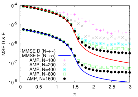
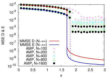
We have tested our algorithm on instances of tractable sizes. The results are shown in Fig. 4 for two noisy cases of matrix calibration. The agreement with the theoretical large $N$ prediction is excellent for small $\pi$. In the large $\pi$ region, however, we observe finite-size corrections going roughly as $\eta/N$. Despite these finite size effect, the MSE reached by the algorithm is excellent in both case. To appreciate the performance of the algorithm, note that a $\ell_{1}$-minimization would give very poor results even with a perfectly known matrix, as the values of $\alpha$ and $\rho$ are above the Donoho-Tanner transition [24].

The presence of $O(\eta/N)$ corrections prevents us from using our algorithm successfully for large $\eta$. This means that so far we are not able to solve efficiently the dictionary learning. More work will be needed to reduce these effects.

IV Perspectives

It would be interesting to see if our result for the MMSE and the exactness of the state evolution can be proven rigorously, as in compressed sensing [25, 23]. Further, it is important to investigate if our algorithm can be improved and the finite size effects reduced. One can also generalize our approach to other matrix decomposition problems and their applications.

References

- [1] I. Carron, “The matrix factorization jungle,” https://sites.google.com/site/igorcarron2/matrixfactorizations.
- [2] B. A. Olshausen and D. J. Field, “Sparse coding with an overcomplete basis set: A strategy employed by v1,” Vision Research, vol. 37, p. 3311, 1997.
- [3] K. Engan, S. O. Aase, and H. J. Husoy, “Method of optimal directions for frame design,” IEEE Acoustic, Speech and Signal Processing, vol. 5, p. 2443, 1999.
- [4] M. Aharon, M. Elad, and A. M. Bruckstein, “K-svd: An algorithm for designing overcomplete dictionaries for sparse representation,” IEEE Transactions on Signal Processing, vol. 54, p. 4311, 2006.
- [5] J. Mairal, F. Bach, J. Ponce, and G. Sapiro, “Online dictionary learning for sparse coding,” in Proceedings of the 26 th International Conference on Machine Learning, Montreal, Canada, 2009., 2009.
- [6] P. Schniter, J. Parker, and V. Cevher, “Bilinear generalized approximate message passing (big-amp) for matrix recovery problem,” in Workshop on Information Theory and Applications (ITA), San Diego CA, 2012.
- [7] A. M. B. Michal Aharon, Michael Elad, “On the uniqueness of overcomplete dictionaries, and a practical way to retrieve them,” Linear Algebra and its Applications, vol. 416, pp. 48–67, 2006.
- [8] R. Gribonval and K. Schnass, “Dictionary identification - sparse matrix-factorisation via -minimisation,” IEEE Transactions on Information Theory, vol. 56, no. 7, pp. 3523–3539, 2010.
- [9] Q. Geng, H. Wang, and J. Wright, “On the local correctness of -minimization for dictionary learning,” 2011, arXiv:1101.5672.
- [10] D. Vainsencher, S. Mannor, and A. M. Bruckstein, “The sample complexity of dictionary learning,” Journal of Machine Learning Research, vol. 12, pp. 3259–3281, 2011.
- [11] A. Sakata and Y. Kabashima, “Statistical mechanics of dictionary learning,” 2012, arXiv:1203.6178.
- [12] R. Gribonval, G. Chardon, and L. Daudet, “Blind calibration for compressed sensing by convex optimization,” in Acoustics, Speech and Signal Processing (ICASSP), 2012 IEEE International Conference on, 2012, pp. 2713 –2716.
- [13] R. Rubinstein, M. Zibulevsky, and M. Elad, “Double sparsity: Learning sparse dictionaries for sparse signal approximation,” IEEE Transactions on Signal Processing, vol. 58, p. 1553, 2010.
- [14] M. Mézard, G. Parisi, and M. A. Virasoro, Spin-Glass Theory and Beyond, ser. Lecture Notes in Physics. Singapore: World Scientific, 1987, vol. 9.
- [15] F. Krzakala, M. Mézard, F. Sausset, Y. Sun, and L. Zdeborová, “Statistical physics-based reconstruction in compressed sensing,” Phys. Rev. X, vol. 2, p. 021005, 2012.
- [16] F. Krzakala, M. Mézard, F. Sausset, Y. Sun, and L. Zdeborová, “Probabilistic reconstruction in compressed sensing: Algorithms, phase diagrams, and threshold achieving matrices,” J. Stat. Mech., vol. P08009, 2012.
- [17] D. L. Donoho, A. Maleki, and A. Montanari, “Message-passing algorithms for compressed sensing,” Proc. Natl. Acad. Sci., vol. 106, no. 45, pp. 18 914–18 919, 2009.
- [18] D. Donoho, A. Maleki, and A. Montanari, “Message passing algorithms for compressed sensing: I. motivation and construction,” in Information Theory Workshop (ITW), 2010 IEEE, 2010, pp. 1 –5.
- [19] S. Rangan, “Generalized approximate message passing for estimation with random linear mixing,” in IEEE International Symposium on Information Theory Proceedings (ISIT), 31 2011-aug. 5 2011, pp. 2168 –2172.
- [20] D. J. Thouless, P. W. Anderson, and R. G. Palmer, “Solution of ‘solvable model of a spin-glass’,” Phil. Mag., vol. 35, pp. 593–601, 1977.
- [21] F. Krzakala, M. Mézard, and L. Zdeborová, “Compressed sensing under matrix uncertainty: Optimum thresholds and robust approximate message passing,” 2012, arXiv:1301.0901 [cs.IT].
- [22] J. Parker, V. Cevher, and P. Schniter, “Compressive sensing under matrix uncertainties: An approximate message passing approach,” in Conference Record of the Forty Fifth Asilomar, 2011.
- [23] M. Bayati and A. Montanari, “The dynamics of message passing on dense graphs, with applications to compressed sensing,” IEEE Transactions on Information Theory, vol. 57, no. 2, pp. 764 –785, 2011.
- [24] D. L. Donoho and J. Tanner, “Sparse nonnegative solution of underdetermined linear equations by linear programming,” Proceedings of the National Academy of Sciences of the United States of America, vol. 102, no. 27, pp. 9446–9451, 2005.
- [25] Y. Wu and S. Verdu, “Optimal phase transitions in compressed sensing,” 2011, arXiv:1111.6822v1 [cs.IT].
- [26] A. Sakata and Y. Kabashima, “Sample complexity of bayesian optimal dictionary learning,” preprint received from the authors.