Self-Propelled Particles with Selective Attraction-Repulsion Interaction - From Microscopic Dynamics to Coarse-Grained Theories

R Großmann1, L Schimansky-Geier1 and P Romanczuk2 1 Department of Physics, Humboldt-Universität zu Berlin, Newtonstr. 15, 12489 Berlin, Germany 2 Max Planck Institute for the Physics of Complex Systems, Nöthnitzerstr. 38, 01187 Dresden, Germany prom@pks.mpg.de
Abstract

In this work we derive and analyze coarse-grained descriptions of self-propelled particles with selective attraction-repulsion interaction, where individuals may respond differently to their neighbours depending on their relative state of motion (approach versus movement away). Based on the formulation of a nonlinear Fokker-Planck equation, we derive a kinetic description of the system dynamics in terms of equations for the Fourier modes of the one-particle density function. This approach allows effective numerical investigation of the stability of solutions of the nonlinear Fokker-Planck equation.

Further on, we also derive a hydrodynamic theory by performing a closure at the level of the second Fourier mode of the one-particle density function. We show that the general form of equations is in agreement with the theory formulated by Toner and Tu. The stability of spatially homogeneous solutions is analyzed and the range of validity of the hydrodynamic equations is quantified.

Finally, we compare our analytical predictions on the stability of the homogeneous solutions with results of individual-based simulations. They show good agreement for sufficiently large densities and non-negligible short-ranged repulsion. The results of the kinetic theory for weak short-ranged repulsion reveal the existence of a previously unknown phase of the model consisting of dense, nematically aligned filaments, which cannot be accounted for by the present hydrodynamics theory of the Toner and Tu type for polar active matter.

pacs:
05.40.Ca, 05.40Jc, 87.10.Mn, 05.70.Ln, 05.20.Dd

1 Introduction

In recent decades, there has been an increased research focus on far-from-equilibrium systems in biology and physics which is referred to as “active matter”. The relevant length scales of such systems span several orders of magnitude. They range from the (sub-)micrometer scale governing the dynamics of individual active units in motility assays in-vitro [1] and the actin cortex in-vivo [2], via the mesoscopic length scales of interest in collective dynamics of large bacterial ensembles [3, 4] and artificial self-propelled particles [5], up to the macroscopic scales of driven granular matter [6, 7] or flocks of birds [8], schools of fish [9], and swarms of insects [10, 11], where the spatial dimensions can be in the order of kilometers.

Despite the apparent variety, all these systems share the fundamental property of local uptake and/or conversion of internal energy into kinetic energy of motion by its individual units. This – together with additional interactions between those units – distinguishes these systems from related equilibrium systems and yields fascinating examples of self-organization and collective dynamics.

The question of universal properties of such active matter systems from the statistical physics point of view is a vibrant research field. To a large extent, it was initiated by the numerical study of a minimal, individual-based model of active matter published by Vicsek et alin 1995 [12]. Shortly after this publication, Toner and Tu made a seminal contribution by formulating the hydrodynamic equations of polar active matter at largest relevant length and time scales purely based on symmetry arguments [13, 14]. The analysis of these generic equations, as well as their counterparts for nematic order, improved our understanding of the fundamental properties of active matter, such as the existence of long range order or giant number fluctuations [15, 16].

However, the direct derivation of a hydrodynamic theory of the Toner and Tu type from microscopic models of active matter was a long standing problem. Only recently, such a link between microscopic parameters determining the dynamics of individual active units and parameters governing the macroscopic flow of active matter was established by formulating kinetic equations for minimal models of self-propelled particles with velocity-alignment [17, 18, 19, 20] and self-propelled aligning rods [21]. Furthermore, coarse-grained descriptions for active particles with variable speeds and velocity-alignment were derived in [22, 23, 24, 25, 26].

In this paper, we will derive a kinetic and a hydrodynamic description for self-propelled agents interacting via a selective attraction and repulsion interaction. A corresponding model was recently introduced to describe the onset of collective motion in insect swarms and is directly motivated by response of individual agents to looming visual stimuli and in particular the distinction of approaching and moving away objects[27, 28].

A fundamental difference of our model and the Vicsek model is its formulation in continuous time using stochastic differential equations. The interaction of individuals are modelled by superposition of (binary) interaction forces. This allows on the one hand a straight forward generalization of the model, e.g. towards variable speed of individuals, and on the other hand can be directly coarse-grained by deriving the Fokker-Planck equation for the corresponding probability density functions. The latter being the main focus of this work.

The model shows different phases including large scale collective motion, a disordered clustering phase and a nematic phase despite the absence of an explicit velocity-alignment interaction.

First, we will introduce the microscopic, individual-based model in terms of stochastic differential equations. Then we will proceed with the discussion of a kinetic description of the collective dynamics based on the nonlinear Fokker-Planck equation for the one-particle density function, which allows efficient numerical analysis of the stability of solutions of the Fokker-Planck equation in Fourier space. Further on, we will derive a hydrodynamic theory for self-propelled particles with selective attraction-repulsion interaction, which yields hydrodynamic equations in agreement with the theory by Toner and Tu. A direct comparison of the kinetic approach, which in principle can be considered up to arbitrary accuracy, to the hydrodynamic theory, which corresponds to a closure at the level of the second Fourier mode of the probability density function, reveals the range of validity of the hydrodynamic equations at large wavenumbers. Moreover, the analysis provides insights into the origin of unphysical divergences at large wavenumbers related to the approximations used namely the usage of Taylor polynomials. Finally, we compare the results of the kinetic and hydrodynamic theory with direct numerical simulations of the individual-based model.

2 Microscopic Model

We consider N𝑁N self-propelled particles of mass m=1𝑚1m=1 in two spatial dimensions, so-called agents. Each individual moves at a constant speed s0subscript𝑠0s_{0}, thus the velocity vector of each agent is determined by its polar orientation angle φisubscript𝜑𝑖\varphi_{i}. The equations of motion for the positions risubscriptri\bi{r}_{i} and the polar orientation angles φisubscript𝜑𝑖\varphi_{i} read:

ritdifferential-dsubscriptridifferential-d𝑡\displaystyle\frac{\rmd\bi{r}_{i}}{\rmd t} =\displaystyle= s0ei,h(t)=s0(𝐜𝐨𝐬𝝋i(t)𝐬𝐢𝐧𝝋i(t)),subscript𝑠0subscripteihtsubscripts0subscript𝝋itsubscript𝝋it\displaystyle s_{0}\bi{e}_{i,h}(t)=s_{0}\!\left(\begin{array}[]{c}\cos\varphi_{i}(t)\\ \sin\varphi_{i}(t)\\ \end{array}\right), (2.1c)
φitdifferential-dsubscript𝜑𝑖differential-d𝑡\displaystyle\frac{\rmd\varphi_{i}}{\rmd t} =\displaystyle= 1s0(Fi,φ+2Dφξi(t)).1subscript𝑠0subscript𝐹𝑖𝜑2subscript𝐷𝜑subscript𝜉𝑖𝑡\displaystyle\frac{1}{s_{0}}\left(F_{i,\varphi}+\sqrt{2D_{\varphi}}\,\xi_{i}(t)\right)\,. (2.1d)

Here, Fi,φ=Fiei,𝝋subscript𝐹𝑖𝜑bold-⋅subscriptFisubscriptei𝝋F_{i,\varphi}=\bi{F}_{i}\cdot\bi{e}_{i,\varphi} is the projection of an effective social force vector FisubscriptFi\bi{F}_{i} on the angular degree of freedom φisubscript𝜑𝑖\varphi_{i}, which induces a turning behaviour of the focal individual due to interaction with others. ei,𝝋=(𝐬𝐢𝐧𝝋i,𝐜𝐨𝐬𝝋i)Tsubscriptei𝝋superscriptsubscript𝝋isubscript𝝋iT\bi{e}_{i,\varphi}=(-\sin\varphi_{i},\cos\varphi_{i})^{T} is the angular unit vector perpendicular to ei,hsubscripteih\bi{e}_{i,h}.

The second term within the brackets in (2.1d) stands for random angular noise with intensity Dφsubscript𝐷𝜑D_{\varphi}. ξi(t)subscript𝜉𝑖𝑡\xi_{i}(t) are independent, Gaussian random processes with vanishing mean and temporal δ𝛿\delta-correlations, i.e. ξi(t)ξj(t+τ)=δijδ(τ)delimited-⟨⟩subscript𝜉𝑖𝑡subscript𝜉𝑗𝑡𝜏subscript𝛿𝑖𝑗𝛿𝜏\left<\xi_{i}(t)\xi_{j}(t+\tau)\right>=\delta_{ij}\,\delta(\tau) (Gaussian white noise).

The total social force is given by a sum of three components:

FisubscriptFi\displaystyle\bi{F}_{i} =fi,r+fi,m+fi,a.absentsubscriptfirsubscriptfimsubscriptfia\displaystyle=\bi{f}_{i,r}+\bi{f}_{i,m}+\bi{f}_{i,a}. (2.1b)

The first term represents a short-ranged repulsion allowing for finite sized agents. It reads

fi,rsubscriptfir\displaystyle\bi{f}_{i,r} =j=1Nμr(rji)^rjiθ(lcrji)absentsuperscriptsubscript𝑗1𝑁subscript𝜇𝑟subscript𝑟𝑗𝑖bold-^absentsubscript𝑟𝑗𝑖𝜃subscript𝑙𝑐subscript𝑟𝑗𝑖\displaystyle=-\sum_{j=1}^{N}\mu_{r}({r}_{ji})\hat{\bi}{r}_{ji}\theta(l_{c}-r_{ji}) (2.1c)

with μr(rji)0subscript𝜇𝑟subscript𝑟𝑗𝑖0\mu_{r}({r}_{ji})\geq 0 being a repulsive turning rate, which in general depends on distance rji=|rji|=|rjri|subscript𝑟𝑗𝑖subscriptrjisubscriptrjsubscriptrir_{ji}=\left|\bi{r}_{ji}\right|=\left|\bi{r}_{j}-\bi{r}_{i}\right| between two particles. We assume that this repulsive interaction is strictly short-ranged, i.e. it vanishes above a finite repulsive radius lcsubscript𝑙𝑐l_{c}, as indicated by the Heaviside (unit-step) function θ(x)𝜃𝑥\theta(x).

The other two forces read:

fi,msubscriptfim\displaystyle\bi{f}_{i,m} =j=1Nμm(rji)^rjiθ(lsrji)θ(rjilc)|v~ji|θ(+v~ji),absentsuperscriptsubscript𝑗1𝑁subscript𝜇𝑚subscript𝑟𝑗𝑖bold-^absentsubscript𝑟𝑗𝑖𝜃subscript𝑙𝑠subscript𝑟𝑗𝑖𝜃subscript𝑟𝑗𝑖subscript𝑙𝑐subscript~𝑣𝑗𝑖𝜃subscript~𝑣𝑗𝑖\displaystyle=\sum_{j=1}^{N}\mu_{m}({r}_{ji})\hat{\bi}{r}_{ji}\theta(l_{s}-r_{ji})\theta(r_{ji}-l_{c})\left|\tilde{v}_{ji}\right|\theta(+\tilde{v}_{ji}), (2.1da)
fi,asubscriptfia\displaystyle\bi{f}_{i,a} =j=1Nμa(rji)^rjiθ(lsrji)θ(rjilc)|v~ji|θ(v~ji).absentsuperscriptsubscript𝑗1𝑁subscript𝜇𝑎subscript𝑟𝑗𝑖bold-^absentsubscript𝑟𝑗𝑖𝜃subscript𝑙𝑠subscript𝑟𝑗𝑖𝜃subscript𝑟𝑗𝑖subscript𝑙𝑐subscript~𝑣𝑗𝑖𝜃subscript~𝑣𝑗𝑖\displaystyle=\sum_{j=1}^{N}\mu_{a}({r}_{ji})\hat{\bi}{r}_{ji}\theta(l_{s}-r_{ji})\theta(r_{ji}-l_{c})\left|\tilde{v}_{ji}\right|\theta(-\tilde{v}_{ji}). (2.1db)

These forces can be considered as a sum over binary interactions, which act always along the unit vector ^rji=(rjri)/rjibold-^absentsubscript𝑟𝑗𝑖subscriptrjsubscriptrisubscriptrji\hat{\bi}{r}_{ji}=(\bi{r}_{j}-\bi{r}_{i})/r_{ji} pointing towards the center of mass of the neighbouring particle j𝑗j. The corresponding response strengths μa,m(rji)subscript𝜇𝑎𝑚subscript𝑟𝑗𝑖\mu_{a,m}(r_{ji}) are distance dependent and may in general be both positive (attraction) and negative (repulsion). Furthermore, the overall response to other individuals is assumed to vanish above a finite sensory range lssubscript𝑙𝑠l_{s}: μa,m(rji>ls)=0subscript𝜇𝑎𝑚subscript𝑟𝑗𝑖subscript𝑙𝑠0\mu_{a,m}(r_{ji}>l_{s})=0, whereby lslcsubscript𝑙𝑠subscript𝑙𝑐l_{s}\geq l_{c}.

Refer to caption
Figure 1: Visualization of the spatial regions for approaching and receding self-propelled particles for a binary interaction of the i𝑖ith particle with velocity vector 𝐯isubscript𝐯𝑖{\bf v}_{i} (heading angle φisubscript𝜑𝑖\varphi_{i}), and a neighbouring particle j𝑗j with velocity 𝐯jsubscript𝐯𝑗{\bf v}_{j} (heading angle φjsubscript𝜑𝑗\varphi_{j}) within its sensory range lssubscript𝑙𝑠l_{s}. The center of the circle corresponds to the position of the focal particle i𝑖i. The dotted line, determined by the mean angle (φi+φj)/2subscript𝜑𝑖subscript𝜑𝑗2(\varphi_{i}+\varphi_{j})/2, represents the border between the two distinct spatial regions (half-discs) corresponding to approaching and moving away of individual j𝑗j. If the j𝑗jth particle is located above the dotted line in the red region, the two particles are coming closer (approaching). Otherwise, if the neighbouring particle is located in the blue region, the two particles move away from each other (as shown in this example).

The decisive factor in the distinction of the two forces is the sign of the relative velocity v~jisubscript~𝑣𝑗𝑖\tilde{v}_{ji} defined by the temporal derivative of the distance r˙jisubscript˙𝑟𝑗𝑖{\dot{r}}_{ji} between particles i𝑖i and j𝑗j, and equals the projection of the velocity difference 𝐯ji=𝐯j𝐯isubscript𝐯𝑗𝑖subscript𝐯𝑗subscript𝐯𝑖{\bf v}_{ji}={\bf v}_{j}-{\bf v}_{i} of neighbour j𝑗j and the focal individual i𝑖i on the relative position unit vector r^jisubscript^r𝑗𝑖\hat{\bi{r}}_{ji}: v~ji=𝐯jir^ji=v~ijsubscript~𝑣𝑗𝑖subscript𝐯𝑗𝑖subscript^r𝑗𝑖subscript~𝑣𝑖𝑗\tilde{v}_{ji}={\bf v}_{ji}\cdot\hat{\bi{r}}_{ji}=\tilde{v}_{ij}. Hence fi,asubscriptfia\bi{f}_{i,a} is the response to approaching individuals characterized by a negative relative velocity v~ji<0subscript~𝑣𝑗𝑖0\tilde{v}_{ji}<0, whereas fi,msubscriptfim\bi{f}_{i,m} is the corresponding response to moving away (or receding) individuals characterized by positive relative velocity v~ji>0subscript~𝑣𝑗𝑖0\tilde{v}_{ji}>0. Both force terms are proportional to the absolute value of the relative velocity, leading to stronger responses to faster approaching or receding individuals. Using the definition v~ji=r˙jisubscript~𝑣𝑗𝑖subscript˙𝑟𝑗𝑖\tilde{v}_{ji}=\dot{r}_{ji}, one obtains the relative velocity

v~ji=v~ji(φi,φj,αji)=2s0sin(φj+φi2αji)sin(φiφj2)subscript~𝑣𝑗𝑖subscript~𝑣𝑗𝑖subscript𝜑𝑖subscript𝜑𝑗subscript𝛼𝑗𝑖2subscript𝑠0subscript𝜑𝑗subscript𝜑𝑖2subscript𝛼𝑗𝑖subscript𝜑𝑖subscript𝜑𝑗2\displaystyle\tilde{v}_{ji}=\tilde{v}_{ji}(\varphi_{i},\varphi_{j},\alpha_{ji})=2{s}_{0}\sin\left(\frac{\varphi_{j}+\varphi_{i}}{2}-\alpha_{ji}\right)\,\sin\left(\frac{\varphi_{i}-\varphi_{j}}{2}\right) (2.1de)

as a function of the velocity angles φisubscript𝜑𝑖\varphi_{i}, φjsubscript𝜑𝑗\varphi_{j} and the angle αjisubscript𝛼𝑗𝑖\alpha_{ji} of the distance vector rjisubscriptrji\bi{r}_{ji}, with rji=rji(𝐜𝐨𝐬𝜶ji,𝐬𝐢𝐧𝜶ji)subscriptrjisubscriptrjisubscript𝜶jisubscript𝜶ji\bi{r}_{ji}=r_{ji}\left(\cos\alpha_{ji},\sin\alpha_{ji}\right). From (2.1de), one finds the two different spatial regions of approaching and receding particles, respectively, where the relative velocity has a different sign for fixed φisubscript𝜑𝑖\varphi_{i} and φjsubscript𝜑𝑗\varphi_{j} in the interval φiφj<φi+2πsubscript𝜑𝑖subscript𝜑𝑗subscript𝜑𝑖2𝜋\varphi_{i}\leq\varphi_{j}<\varphi_{i}+2\pi:

v~ji>0forφj+φi2<αji<φj+φi2+πmoving away,v~ji<0forφj+φi2+π<αji<φj+φi2+2πapproaching.subscript~𝑣𝑗𝑖0forsubscript𝜑𝑗subscript𝜑𝑖2absentsubscript𝛼𝑗𝑖absentsubscript𝜑𝑗subscript𝜑𝑖2𝜋moving away,subscript~𝑣𝑗𝑖0forsubscript𝜑𝑗subscript𝜑𝑖2𝜋absentsubscript𝛼𝑗𝑖absentsubscript𝜑𝑗subscript𝜑𝑖22𝜋approaching.\displaystyle\begin{array}[]{c c r c l c}\tilde{v}_{ji}>0&\mbox{for}&\frac{\varphi_{j}+\varphi_{i}}{2}&<\alpha_{ji}<&\frac{\varphi_{j}+\varphi_{i}}{2}+\pi&\mbox{moving away,}\\ \tilde{v}_{ji}<0&\mbox{for}&\frac{\varphi_{j}+\varphi_{i}}{2}+\pi&<\alpha_{ji}<&\frac{\varphi_{j}+\varphi_{i}}{2}+2\pi&\mbox{approaching.}\end{array} (2.1dh)

Hence, a particle located in the half-sphere in clockwise direction from the mean angle (φj+φi)/2subscript𝜑𝑗subscript𝜑𝑖2(\varphi_{j}+\varphi_{i})/2 approaches the focal particle i𝑖i, whereas particles located in the other half-sphere anticlockwise from the mean angle are moving away (see figure 1). Please note that for φj=φisubscript𝜑𝑗subscript𝜑𝑖\varphi_{j}=\varphi_{i} the social force vanishes as v~ji=0subscript~𝑣𝑗𝑖0\tilde{v}_{ji}=0 according to (2.1de).

Four different regions in the (μm,μa)subscript𝜇𝑚subscript𝜇𝑎(\mu_{m},\mu_{a})-parameter space are distinguished [28]:

  • pure attraction: μm>0subscript𝜇𝑚0\mu_{m}>0, μa>0subscript𝜇𝑎0\mu_{a}>0;

  • effective alignment: μm>0subscript𝜇𝑚0\mu_{m}>0, μa<0subscript𝜇𝑎0\mu_{a}<0, i.e. attraction to particles moving away, repulsion from particles coming closer;

  • pure repulsion: μm<0subscript𝜇𝑚0\mu_{m}<0, μa<0subscript𝜇𝑎0\mu_{a}<0;

  • effective anti-alignment: μm<0subscript𝜇𝑚0\mu_{m}<0, μa>0subscript𝜇𝑎0\mu_{a}>0, i.e. attraction to particles coming closer, repulsion from particles moving away.

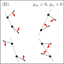
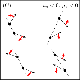
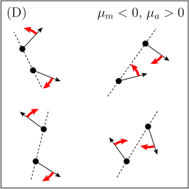
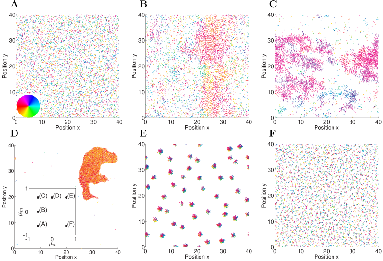
Some typical spatial snapshots obtained from individual-based simulations of (2) are shown in figure 2. A schematic visualisation of the turning behavior of interacting agents in the different regimes is shown in A.

Please note that in previous publications [27, 28], the “effective alignment” regime was referred to as “escape and pursuit”, whereas “effective anti-alignment” was labelled “head on head”. These previous labels had their origin in the context of heterogeneous agents and the respective response of individual agents to neighbors irrespective on their behavior. Furthermore, an asymmetric alignment response for μm>0subscript𝜇𝑚0\mu_{m}>0, μa<0subscript𝜇𝑎0\mu_{a}<0, yields in the present model the same qualitative dependence of the observed spatial patterns on the interaction strengths as in the original “escape and pursuit” model [33]. Nevertheless, for self-propelled agents with constant speed, the above labels appear more appropriate.

One could argue, that in the effective alignment regime the macroscopic dynamics is essentially identical to other models, as for example the minimal Vicsek-model. However, for strong attraction to particles moving away in comparison to the repulsion to approaching particles, we observe the emergence of dense, collectively moving clusters, which do not appear in simple alignment models.
Refer to caption
Figure 2: Spatial snapshots of the microscopic model for different interaction strengths after the system relaxes towards a steady-state: (A) disordered, homogeneous state for μa=μm=0.6subscript𝜇𝑎subscript𝜇𝑚0.6\mu_{a}=\mu_{m}=-0.6 (pure repulsion), (B) diffuse collectively moving bands for μa=0.6subscript𝜇𝑎0.6\mu_{a}=-0.6, μm=0subscript𝜇𝑚0\mu_{m}=0 (repulsion from approaching individuals), (C) collectively moving bands for μa=0.6subscript𝜇𝑎0.6\mu_{a}=-0.6, μm=0.6subscript𝜇𝑚0.6\mu_{m}=0.6 (effective alignment), (D) dense, collectively moving cluster for μm=0.6subscript𝜇𝑚0.6\mu_{m}=0.6, μa=0subscript𝜇𝑎0\mu_{a}=0 (attraction to individuals moving away), (E) cluster state for μm=μa=0.6subscript𝜇𝑚subscript𝜇𝑎0.6\mu_{m}=\mu_{a}=0.6 (pure attraction), (F) disordered, homogeneous state for μm=0.6subscript𝜇𝑚0.6\mu_{m}=-0.6, μa=0.6subscript𝜇𝑎0.6\mu_{a}=0.6 (effective anti-alignment). The velocity vectors of individual particles are coloured corresponding to their polar direction of motion according to the inset of (A). The inset in (D) indicates the positions of the snapshots in the (μm,μa)subscript𝜇𝑚subscript𝜇𝑎(\mu_{m},\mu_{a})-parameter plane. Other parameters: N=4000𝑁4000N=4000, L=40𝐿40L=40, Dφ=0.02subscript𝐷𝜑0.02D_{\varphi}=0.02, ls=1subscript𝑙𝑠1l_{s}=1, lc=0.2subscript𝑙𝑐0.2l_{c}=0.2, μr=5subscript𝜇𝑟5\mu_{r}=5, s0=0.25subscript𝑠00.25s_{0}=0.25.

Our model corresponds to the ones studied in [27, 28], if the distance dependent interaction strengths μr(rji)subscript𝜇𝑟subscript𝑟𝑗𝑖\mu_{r}(r_{ji}) and μa,m(rji)subscript𝜇𝑎𝑚subscript𝑟𝑗𝑖\mu_{a,m}(r_{ji}) are assumed to be constant and the forces are rescaled by the number of particles within the interaction area of the focal particle.

3 Kinetic Description

3.1 Mean-Field Theory - Derivation and Analysis of a Nonlinear Fokker-Planck Equation

In this section, we derive a kinetic description for the above individual-based model (2). For this purpose, we introduce the N𝑁N-particle probability density function (PDF)

PN(r1,𝝋1;r2,𝝋2;;rN,𝝋N;t),subscript𝑃𝑁subscriptr1subscript𝝋1subscriptr2subscript𝝋2bold-…subscriptrNsubscript𝝋Nt\displaystyle P_{N}(\bi{r}_{1},\varphi_{1};\bi{r}_{2},\varphi_{2};\ldots;\bi{r}_{N},\varphi_{N};t)\,, (2.1da)

which determines the probability to find particle i𝑖i at position risubscriptri\bi{r}_{i} moving into the direction φisubscript𝜑𝑖\varphi_{i} (i=1,2,,N𝑖12𝑁i=1,2,\ldots,N) at time t𝑡t. It is normalized with respect to integration over all positions and angles:

[j=1N(2rj02πφj)]PN(r1,𝝋1;r2,𝝋2;;rN,𝝋N;t)=1.delimited-[]superscriptsubscriptproduct𝑗1𝑁superscriptdifferential-d2subscript𝑟𝑗superscriptsubscript02𝜋differential-dsubscript𝜑𝑗subscript𝑃𝑁subscriptr1subscript𝝋1subscriptr2subscript𝝋2bold-…subscriptrNsubscript𝝋Nt1\displaystyle\left[\;\prod_{j=1}^{N}\left(\int\rmd^{2}r_{j}\int_{0}^{2\pi}\rmd\varphi_{j}\right)\right]P_{N}(\bi{r}_{1},\varphi_{1};\bi{r}_{2},\varphi_{2};\ldots;\bi{r}_{N},\varphi_{N};t)=1\,. (2.1db)

In agreement with (2), we can write down the Fokker-Planck equation (FPE) for the dynamics of the PDF as follows.

PNt=s0i=1Nri(ei,hPN)i=1Nφi(Fi,φPNs0)+Dφs02i=1N2PNφi2subscript𝑃𝑁𝑡subscript𝑠0superscriptsubscript𝑖1𝑁subscriptsubscriptrisubscripteihsubscriptPNsuperscriptsubscript𝑖1𝑁subscript𝜑𝑖subscript𝐹𝑖𝜑subscript𝑃𝑁subscript𝑠0subscript𝐷𝜑superscriptsubscript𝑠02superscriptsubscript𝑖1𝑁superscript2subscript𝑃𝑁superscriptsubscript𝜑𝑖2\displaystyle\frac{\partial P_{N}}{\partial t}=-s_{0}\sum_{i=1}^{N}\nabla_{\bi{r}_{i}}\cdot\left(\bi{e}_{i,h}P_{N}\right)-\sum_{i=1}^{N}\frac{\partial}{\partial\varphi_{i}}\left(\frac{F_{i,\varphi}\,P_{N}}{s_{0}}\right)+\frac{D_{\varphi}}{s_{0}^{2}}\sum_{i=1}^{N}\frac{\partial^{2}P_{N}}{\partial\varphi_{i}^{2}} (2.1dc)

From the linear FPE above one can derive an evolution equation for the marginal PDF

P(ri,𝝋i,t)=[jiN(2rj02𝝅𝝋j)]PN(r1,𝝋1;r2,𝝋2;;rN,𝝋N;t)𝑃subscriptrisubscript𝝋itdelimited-[]superscriptsubscriptproductjiNsuperscriptdifferential-d2subscriptrjsuperscriptsubscript02𝝅differential-dsubscript𝝋jsubscriptPNsubscriptr1subscript𝝋1subscriptr2subscript𝝋2bold-…subscriptrNsubscript𝝋Nt\displaystyle P(\bi{r}_{i},\varphi_{i},t)=\left[\;\prod_{j\neq i}^{N}\left(\int\rmd^{2}r_{j}\int_{0}^{2\pi}\rmd\varphi_{j}\right)\right]P_{N}(\bi{r}_{1},\varphi_{1};\bi{r}_{2},\varphi_{2};\ldots;\bi{r}_{N},\varphi_{N};t) (2.1dd)

by integrating (2.1dc) over the degrees of freedom of particles ji𝑗𝑖j\neq i. In what follows, we assume that correlations between particles can be neglected. Therefore, the N𝑁N-particle PDF factorizes, i.e.

PN(r1,𝝋1;r2,𝝋2;;rN,𝝋N;t)=i=1NP(ri,𝝋i,t).subscript𝑃𝑁subscriptr1subscript𝝋1subscriptr2subscript𝝋2bold-…subscriptrNsubscript𝝋Ntsuperscriptsubscriptproducti1NPsubscriptrisubscript𝝋it\displaystyle P_{N}(\bi{r}_{1},\varphi_{1};\bi{r}_{2},\varphi_{2};\ldots;\bi{r}_{N},\varphi_{N};t)=\prod_{i=1}^{N}P(\bi{r}_{i},\varphi_{i},t). (2.1de)

By this means, one obtains an effective one-particle description

P(ri,𝝋i,t)t=s0ri(ei,hP)N1s0φi(FφP)+Dφs022Pφi2,𝑃subscriptrisubscript𝝋it𝑡subscript𝑠0subscriptsubscriptrisubscripteihP𝑁1subscript𝑠0subscript𝜑𝑖subscript𝐹𝜑𝑃subscript𝐷𝜑superscriptsubscript𝑠02superscript2𝑃superscriptsubscript𝜑𝑖2\displaystyle\frac{\partial P(\bi{r}_{i},\varphi_{i},t)}{\partial t}=-s_{0}\nabla_{\bi{r}_{i}}\cdot\left(\bi{e}_{i,h}P\right)-\frac{N-1}{s_{0}}\frac{\partial}{\partial\varphi_{i}}\left(F_{\varphi}\,P\right)+\frac{D_{\varphi}}{s_{0}^{2}}\frac{\partial^{2}P}{\partial\varphi_{i}^{2}}\,, (2.1df)

where the force Fφsubscript𝐹𝜑F_{\varphi} is given by the following integral over P(ri,𝝋i,t)𝑃subscriptrisubscript𝝋itP(\bi{r}_{i},\varphi_{i},t):

Fφsubscript𝐹𝜑\displaystyle F_{\varphi} (ri,𝝋i,t)=2s0𝝋i𝝋i+2𝝅d𝝋j𝐬𝐢𝐧(𝝋i𝝋j2)lclsdrjirjisubscriptrisubscript𝝋it2subscripts0superscriptsubscriptsubscript𝝋isubscript𝝋i2𝝅dsubscript𝝋jsubscript𝝋isubscript𝝋j2superscriptsubscriptsubscriptlcsubscriptlsdsubscriptrjisubscriptrji\displaystyle(\bi{r}_{i},\varphi_{i},t)=2s_{0}\int_{\varphi_{i}}^{\varphi_{i}+2\pi}\mbox{d}\varphi_{j}\,\sin\left(\frac{\varphi_{i}-\varphi_{j}}{2}\right)\int_{l_{c}}^{l_{s}}\mbox{d}r_{ji}\,r_{ji} (2.1dg)
[μm(rji)φi+φj2φi+φj2+πdαjisin(αjiφi)sin(φi+φj2αji)P(ri+rji,𝝋j,t)\displaystyle\left[\mu_{m}(r_{ji})\int_{\frac{\varphi_{i}+\varphi_{j}}{2}}^{\frac{\varphi_{i}+\varphi_{j}}{2}+\pi}\mbox{d}\alpha_{ji}\,\sin(\alpha_{ji}-\varphi_{i})\sin\left(\frac{\varphi_{i}+\varphi_{j}}{2}-\alpha_{ji}\right)P(\bi{r}_{i}+\bi{r}_{ji},\varphi_{j},t)\right.
μa(rji)φi+φj2+πφi+φj2+2πdαjisin(αjiφi)sin(φi+φj2αji)P(ri+rji,𝝋j,t)]\displaystyle\left.-\mu_{a}(r_{ji})\int_{\frac{\varphi_{i}+\varphi_{j}}{2}+\pi}^{\frac{\varphi_{i}+\varphi_{j}}{2}+2\pi}\mbox{d}\alpha_{ji}\,\sin(\alpha_{ji}-\varphi_{i})\sin\left(\frac{\varphi_{i}+\varphi_{j}}{2}-\alpha_{ji}\right)P(\bi{r}_{i}+\bi{r}_{ji},\varphi_{j},t)\right]
φiφi+2πdφj0lcdrjirji02πdαjiμr(rji)sin(αjiφi)P(ri+rji,𝝋j,t).superscriptsubscriptsubscript𝜑𝑖subscript𝜑𝑖2𝜋dsubscript𝜑𝑗superscriptsubscript0subscript𝑙𝑐dsubscript𝑟𝑗𝑖subscript𝑟𝑗𝑖superscriptsubscript02𝜋dsubscript𝛼𝑗𝑖subscript𝜇𝑟subscript𝑟𝑗𝑖subscript𝛼𝑗𝑖subscript𝜑𝑖𝑃subscriptrisubscriptrjisubscript𝝋jt\displaystyle-\int_{\varphi_{i}}^{\varphi_{i}+2\pi}\mbox{d}\varphi_{j}\int_{0}^{l_{c}}\mbox{d}r_{ji}\,r_{ji}\int_{0}^{2\pi}\mbox{d}\alpha_{ji}\,\mu_{r}(r_{ji})\sin(\alpha_{ji}-\varphi_{i})P(\bi{r}_{i}+\bi{r}_{ji},\varphi_{j},t)\,.

The factor N1𝑁1N-1 in (2.1df) arises, because (2.1dc) was integrated over the positions and angles of N1𝑁1N-1 identical particles. In other words, the focal particle can interact with N1𝑁1N-1 identical neighbours. For the same reason, the particle index i𝑖i is omitted henceforward.

The FPE (2.1df), which was derived from the linear FPE (2.1dc) governing the dynamics of PNsubscript𝑃𝑁P_{N}, is nonlinear since the force terms Fφsubscript𝐹𝜑F_{\varphi} depend on P(r,𝝋,t)𝑃r𝝋tP(\bi{r},\varphi,t). In this sense, assumption (2.1de) is a mean-field approximation: a single particle is affected by a force due to its own PDF (2.1dg).

By introducing the one-particle density function p(r,𝝋,t)=NP(r,𝝋,t)𝑝r𝝋tNPr𝝋tp(\bi{r},\varphi,t)=NP(\bi{r},\varphi,t) we can eliminate the factor (N1)N𝑁1𝑁(N-1)\approx N from (2.1df). Accordingly, p(r,𝝋,t)𝑝r𝝋tp(\bi{r},\varphi,t) is interpreted as particle density obeying the nonlinear Fokker-Planck equation

p(r,𝝋,t)t=s0r(ehp)φFφ(r,𝝋,t)ps0+Dφs022pφ2.𝑝r𝝋t𝑡subscript𝑠0subscriptrsubscriptehp𝜑subscript𝐹𝜑r𝝋tpsubscript𝑠0subscript𝐷𝜑superscriptsubscript𝑠02superscript2𝑝superscript𝜑2\displaystyle\frac{\partial p(\bi{r},\varphi,t)}{\partial t}=-s_{0}\nabla_{\bi{r}}\cdot\left(\bi{e}_{h}\,p\right)-\frac{\partial}{\partial\varphi}\frac{F_{\varphi}(\bi{r},\varphi,t)\,p}{s_{0}}+\frac{D_{\varphi}}{s_{0}^{2}}\frac{\partial^{2}p}{\partial\varphi^{2}}\,. (2.1dh)

First, we assume a spatially homogeneous situation where p(r,𝝋,t)=p(𝝋,t)𝑝r𝝋tp𝝋tp(\bi{r},\varphi,t)=p(\varphi,t) holds. In this case, (2.1dh) is reduced to

p(φ,t)t=Dφs02φ[κρ0φφ+2πφjsin(φjφ)p(φj,t)p(φ,t)pφ],𝑝𝜑𝑡𝑡subscript𝐷𝜑superscriptsubscript𝑠02𝜑delimited-[]𝜅subscript𝜌0superscriptsubscript𝜑𝜑2𝜋differential-dsubscript𝜑𝑗subscript𝜑𝑗𝜑𝑝subscript𝜑𝑗𝑡𝑝𝜑𝑡𝑝𝜑\displaystyle\frac{\partial p(\varphi,t)}{\partial t}=-\frac{D_{\varphi}}{s_{0}^{2}}\frac{\partial}{\partial\varphi}\left[\frac{\kappa}{\rho_{0}}\,\,\int_{\varphi}^{\varphi+2\pi}\rmd\varphi_{j}\,\sin(\varphi_{j}-\varphi)p(\varphi_{j},t)\,p(\varphi,t)-\frac{\partial p}{\partial\varphi}\right]\,, (2.1di)

where the dimensionless coupling parameter

κ=πρ0s022Dφlclsrjirji(μm(rji)μa(rji))𝜅𝜋subscript𝜌0superscriptsubscript𝑠022subscript𝐷𝜑superscriptsubscriptsubscript𝑙𝑐subscript𝑙𝑠differential-dsubscript𝑟𝑗𝑖subscript𝑟𝑗𝑖subscript𝜇𝑚subscript𝑟𝑗𝑖subscript𝜇𝑎subscript𝑟𝑗𝑖\displaystyle\kappa=\frac{\pi\rho_{0}s_{0}^{2}}{2D_{\varphi}}\int_{l_{c}}^{l_{s}}\rmd r_{ji}\,r_{ji}\left(\mu_{m}(r_{ji})-\mu_{a}(r_{ji})\right) (2.1dj)

is introduced, where ρ0=N/L2subscript𝜌0𝑁superscript𝐿2\rho_{0}=N/L^{2} is the homogeneous particle density, with L𝐿L being the linear spatial dimension of the two-dimensional square-shaped system.

One obtains the same Fokker-Planck equation as (2.1di) for self-propelled particles interacting via a velocity-alignment mechanism or globally coupled Kuramoto oscillators [36, 37]. Hence, the selective attraction-repulsion interaction reduces to effective velocity-alignment as considered in [38] (continuum time form of the original Vicsek model [12]), if spatial inhomogeneities are neglected. Furthermore, the effective alignment strength is proportional to μmμasubscript𝜇𝑚subscript𝜇𝑎\mu_{m}-\mu_{a} and may be negative, leading to anti-alignment as a consequence of repulsion from particles moving away and attraction to particles coming closer, respectively (see also figure 10(D)).

The spatially homogeneous, time-independent particle density

p(Φ)(φ)=ρ02πexp(κΦcos(φφ0))I0(κΦ)superscript𝑝Φ𝜑subscript𝜌02𝜋𝜅Φ𝜑subscript𝜑0subscript𝐼0𝜅Φ\displaystyle p^{(\Phi)}(\varphi)=\frac{\rho_{0}}{2\pi}\,\frac{\exp\left(\kappa\Phi\cos(\varphi-\varphi_{0})\right)}{I_{0}(\kappa\Phi)} (2.1dk)

is a solution to both nonlinear Fokker-Planck equations (2.1dh) and (2.1di), as can be easily shown by inserting (2.1dk) into (2.1di). Iν(x)subscript𝐼𝜈𝑥I_{\nu}(x) denotes the modified Bessel-function of the first kind. Without loss of generality, we choose the frame of reference such that the direction of collective motion φ0subscript𝜑0\varphi_{0} defines the x-coordinate, i.e. φ0=0subscript𝜑00\varphi_{0}=0. From the definition of the polar order parameter

ΦΦ\displaystyle\Phi =\displaystyle= |eiφ|=|02π𝑑φp(Φ)(φ)eiφ|delimited-⟨⟩superscript𝑒𝑖𝜑superscriptsubscript02𝜋differential-d𝜑superscript𝑝Φ𝜑superscript𝑒𝑖𝜑\displaystyle\left|\left<e^{i\varphi}\right>\right|=\left|\int_{0}^{2\pi}d\varphi\,p^{(\Phi)}(\varphi)e^{i\varphi}\right| (2.1dl)

we can determine the order parameter by solving the transcendental equation

ΦΦ\displaystyle\Phi =\displaystyle= I1(κΦ)I0(κΦ).subscript𝐼1𝜅Φsubscript𝐼0𝜅Φ\displaystyle\frac{I_{1}(\kappa\Phi)}{I_{0}(\kappa\Phi)}\ . (2.1dm)

Equation (2.1dm) is always fulfilled for Φ=0Φ0\Phi=0. In that case, (2.1dk) yields the uniform distribution (spatially homogeneous, disordered state), i.e.

p(0)=ρ02π.superscript𝑝0subscript𝜌02𝜋\displaystyle p^{(0)}=\frac{\rho_{0}}{2\pi}\,. (2.1dn)

If κ>2𝜅2\kappa>2 (high effective alignment strength μmμasubscript𝜇𝑚subscript𝜇𝑎\mu_{m}-\mu_{a} and low noise Dφsubscript𝐷𝜑D_{\varphi}, respectively), there is a second nontrivial solution Φ>0Φ0\Phi>0 to (2.1dm) describing a spatially homogeneous state with polar order (collective motion; swarming phase). In this parameter region, the distribution p(Φ)superscript𝑝Φp^{(\Phi)} describing polar order (Φ>0Φ0\Phi>0) is stable with respect to spatially homogeneous perturbations δp=δp(φ,t)𝛿𝑝𝛿𝑝𝜑𝑡\delta p=\delta p(\varphi,t), whereas the homogeneous distribution p(0)superscript𝑝0p^{(0)} is stable for κ<2𝜅2\kappa<2 [36, 37].

The critical line κ=2𝜅2\kappa=2 for the order-disorder transition is translated to microscopic model parameters as follows:

lclsrjirji(μm(rji)μa(rji))=4Dφπρ0s02.superscriptsubscriptsubscript𝑙𝑐subscript𝑙𝑠differential-dsubscript𝑟𝑗𝑖subscript𝑟𝑗𝑖subscript𝜇𝑚subscript𝑟𝑗𝑖subscript𝜇𝑎subscript𝑟𝑗𝑖4subscript𝐷𝜑𝜋subscript𝜌0superscriptsubscript𝑠02.\displaystyle\int_{l_{c}}^{l_{s}}\rmd r_{ji}\,r_{ji}\left(\mu_{m}(r_{ji})-\mu_{a}(r_{ji})\right)=\frac{4D_{\varphi}}{\pi\rho_{0}s_{0}^{2}}\,\mbox{. } (2.1do)

The above is a generalization of the previous result obtained in [28]. Since the order-disorder transition described by (2.1dm) is continuous, the right hand side of (2.1dm) can be expanded in a Taylor series so that the dependence Φ=Φ(κ)ΦΦ𝜅\Phi=\Phi(\kappa) is known close to the critical point κc=2subscript𝜅𝑐2\kappa_{c}=2 analytically:

Φ(κ)κ2+𝒪((k2)3/2).similar-to-or-equalsΦ𝜅𝜅2𝒪superscript𝑘232\displaystyle\Phi(\kappa)\simeq\sqrt{\kappa-2}+\mathcal{O}\left((k-2)^{3/2}\right)\,. (2.1dp)

The stability analysis of the spatially homogeneous solutions p(Φ)superscript𝑝Φp^{(\Phi)} with respect to arbitrary perturbations δp=δp(r,𝝋,t)𝛿𝑝𝛿𝑝r𝝋t\delta p=\delta p(\bi{r},\varphi,t) is carried out in the next section.

3.2 Stability Analysis in Fourier Space

In this section it is shown, how the stability of solutions of the nonlinear Fokker-Planck equation (2.1dh) can be analyzed in Fourier space. A similar approach was used by Chou et alin order to achieve a kinetic theory for self-propelled particles with metric-free interactions [29].

In order to analyze the Fokker-Planck equation (2.1dh) analytically and especially to solve the integral (2.1dg), it is convenient to work in Fourier space with respect to the spatial coordinates rr\bi{r} and the angular variable φ𝜑\varphi. The dynamics of the Fourier coefficients

g^n(k,t)=2r02𝝅𝝋p(r,𝝋,t)eikr+in𝝋subscript^𝑔𝑛ktsuperscriptdifferential-d2rsuperscriptsubscript02𝝅differential-d𝝋pr𝝋tsuperscriptebold-⋅ikrin𝝋\displaystyle{\hat{g}}_{n}(\bi{k},t)=\int\rmd^{2}r\int_{0}^{2\pi}\rmd\varphi\,p(\bi{r},\varphi,t)e^{i\bi{k}\cdot\bi{r}+in\varphi} (2.1dq)

reads

g^n(k,t)tikxs02(g^n+1+g^n1)kys02(g^n+1g^n1)=n2Dφs02g^nsubscript^𝑔𝑛kt𝑡𝑖subscript𝑘𝑥subscript𝑠02subscript^𝑔𝑛1subscript^𝑔𝑛1subscript𝑘𝑦subscript𝑠02subscript^𝑔𝑛1subscript^𝑔𝑛1superscript𝑛2subscript𝐷𝜑superscriptsubscript𝑠02subscript^𝑔𝑛\displaystyle\frac{\partial{\hat{g}}_{n}(\bi{k},t)}{\partial t}-\frac{ik_{x}s_{0}}{2}\left({\hat{g}}_{n+1}+{\hat{g}}_{n-1}\right)-\frac{k_{y}s_{0}}{2}\left({\hat{g}}_{n+1}-{\hat{g}}_{n-1}\right)=-n^{2}\frac{D_{\varphi}}{s_{0}^{2}}{\hat{g}}_{n}
+in(2π)3s0j=2qg^j(q,t)K^nj(kq,t),𝑖𝑛superscript2𝜋3subscript𝑠0superscriptsubscript𝑗superscriptdifferential-d2𝑞subscript^𝑔𝑗qtsubscriptbold-^Knjkqt\displaystyle+\frac{in}{(2\pi)^{3}s_{0}}\sum_{j=-\infty}^{\infty}\int\rmd^{2}q\,{\hat{g}}_{j}(\bi{q},t){\hat{K}}_{n-j}(\bi{k}-\bi{q},t)\,, (2.1dr)

where the Fourier coefficients of the force (2.1dg) are defined as

K^n(k,t)=2r02𝝅𝝋F𝝋(r,𝝋,t)eikr+in𝝋.subscript^𝐾𝑛ktsuperscriptdifferential-d2rsuperscriptsubscript02𝝅differential-d𝝋subscriptF𝝋r𝝋tsuperscriptebold-⋅ikrin𝝋\displaystyle{\hat{K}}_{n}(\bi{k},t)=\int\rmd^{2}r\int_{0}^{2\pi}\rmd\varphi\,F_{\varphi}(\bi{r},\varphi,t)e^{i\bi{k}\cdot\bi{r}+in\varphi}\,. (2.1ds)

Obviously, the Fokker-Planck equation turns into an infinite hierarchy of equations (3.2) in Fourier space.

For the stability analysis, the Fourier coefficients K^n(k,t)subscript^𝐾𝑛kt{\hat{K}}_{n}(\bi{k},t) of the force (2.1dg) are required. Due to the fact, that the force Fφ(r,𝝋,t)subscript𝐹𝜑r𝝋tF_{\varphi}(\bi{r},\varphi,t) depends on the integral over p(r,𝝋,t)𝑝r𝝋tp(\bi{r},\varphi,t) (2.1dg), the Fourier coefficients K^n(k,t)subscript^𝐾𝑛kt{\hat{K}}_{n}(\bi{k},t) of the force can be written as a linear combination of the Fourier coefficients g^r(k,t)subscript^𝑔𝑟kt{\hat{g}}_{r}(\bi{k},t)

K^n(k,t)=r=K~n,r(k)g^r(k,t)subscript^𝐾𝑛ktsuperscriptsubscriptrsubscriptbold-~Knrksubscriptbold-^grkt\displaystyle{\hat{K}}_{n}(\bi{k},t)=\sum_{r=-\infty}^{\infty}\tilde{K}_{n,r}(\bi{k})\,{\hat{g}}_{r}(\bi{k},t) (2.1dt)

using an infinite dimensional matrix K~n,r(k)subscript~𝐾𝑛𝑟k\tilde{K}_{n,r}(\bi{k}). Details on the calculation of the matrix elements are given in B. Consequently, the dynamics of the Fourier coefficients g^n(k,t)subscript^𝑔𝑛kt{\hat{g}}_{n}(\bi{k},t) read

g^n(k,t)tikxs02(g^n+1+g^n1)kys02(g^n+1g^n1)=n2Dφs02g^nsubscript^𝑔𝑛kt𝑡𝑖subscript𝑘𝑥subscript𝑠02subscript^𝑔𝑛1subscript^𝑔𝑛1subscript𝑘𝑦subscript𝑠02subscript^𝑔𝑛1subscript^𝑔𝑛1superscript𝑛2subscript𝐷𝜑superscriptsubscript𝑠02subscript^𝑔𝑛\displaystyle\frac{\partial{\hat{g}}_{n}(\bi{k},t)}{\partial t}-\frac{ik_{x}s_{0}}{2}\left({\hat{g}}_{n+1}+{\hat{g}}_{n-1}\right)-\frac{k_{y}s_{0}}{2}\left({\hat{g}}_{n+1}-{\hat{g}}_{n-1}\right)=-n^{2}\frac{D_{\varphi}}{s_{0}^{2}}{\hat{g}}_{n}
+in(2π)3s0j=r=2qg^j(q,t)g^r(kq,t)K~nj,r(kq).𝑖𝑛superscript2𝜋3subscript𝑠0superscriptsubscript𝑗superscriptsubscript𝑟superscriptdifferential-d2𝑞subscript^𝑔𝑗qtsubscriptbold-^grkqtsubscriptbold-~Knjrkq\displaystyle+\frac{in}{(2\pi)^{3}s_{0}}\sum_{j=-\infty}^{\infty}\sum_{r=-\infty}^{\infty}\int\rmd^{2}q\,{\hat{g}}_{j}(\bi{q},t){\hat{g}}_{r}(\bi{k}-\bi{q},t)\tilde{K}_{n-j,r}(\bi{k}-\bi{q})\,. (2.1du)

Let g^n(0)(k,t)superscriptsubscript^𝑔𝑛0kt{\hat{g}}_{n}^{(0)}(\bi{k},t) be a solution of the equation above. The dynamics of a small perturbation δg^n(k,t)=g^n(k,t)g^n(0)(k,t)𝛿subscript^𝑔𝑛ktsubscriptbold-^gnktsuperscriptsubscriptbold-^gn0kt\delta{\hat{g}}_{n}(\bi{k},t)={\hat{g}}_{n}(\bi{k},t)-{\hat{g}}_{n}^{(0)}(\bi{k},t) is determined by the linearized equation

δg^n(k,t)tikxs02(δg^n+1+δg^n1)kys02(δg^n+1δg^n1)=n2Dφs02δg^n+in(2π)3s0𝛿subscript^𝑔𝑛kt𝑡𝑖subscript𝑘𝑥subscript𝑠02𝛿subscript^𝑔𝑛1𝛿subscript^𝑔𝑛1subscript𝑘𝑦subscript𝑠02𝛿subscript^𝑔𝑛1𝛿subscript^𝑔𝑛1superscript𝑛2subscript𝐷𝜑superscriptsubscript𝑠02𝛿subscript^𝑔𝑛𝑖𝑛superscript2𝜋3subscript𝑠0\displaystyle\frac{\partial\delta{\hat{g}}_{n}(\bi{k},t)}{\partial t}-\frac{ik_{x}s_{0}}{2}\left(\delta{\hat{g}}_{n+1}+\delta{\hat{g}}_{n-1}\right)-\frac{k_{y}s_{0}}{2}\left(\delta{\hat{g}}_{n+1}-\delta{\hat{g}}_{n-1}\right)=-n^{2}\frac{D_{\varphi}}{s_{0}^{2}}\delta{\hat{g}}_{n}+\frac{in}{(2\pi)^{3}s_{0}}
j=r=2q(δg^j(q,t)g^r(0)(kq,t)+g^j(0)(q,t)𝜹g^r(kq,t))K~nj,r(kq).superscriptsubscript𝑗superscriptsubscript𝑟superscriptdifferential-d2𝑞𝛿subscript^𝑔𝑗qtsuperscriptsubscriptbold-^gr0kqtsuperscriptsubscriptbold-^gj0qt𝜹subscriptbold-^grkqtsubscript~𝐾𝑛𝑗𝑟kq\displaystyle\sum_{j=-\infty}^{\infty}\sum_{r=-\infty}^{\infty}\int\rmd^{2}q\,\left(\delta{\hat{g}}_{j}(\bi{q},t){\hat{g}}_{r}^{(0)}(\bi{k}-\bi{q},t)+{\hat{g}}_{j}^{(0)}(\bi{q},t)\delta{\hat{g}}_{r}(\bi{k}-\bi{q},t)\right)\tilde{K}_{n-j,r}(\bi{k}-\bi{q}). (2.1dv)

The stability analysis of the solutions

p(Φ)(φ)=ρ02πexp(κΦcosφ)I0(κΦ)superscript𝑝Φ𝜑subscript𝜌02𝜋𝜅Φ𝜑subscript𝐼0𝜅Φ\displaystyle p^{(\Phi)}(\varphi)=\frac{\rho_{0}}{2\pi}\,\frac{\exp\left(\kappa\Phi\cos\varphi\right)}{I_{0}(\kappa\Phi)} (2.1dw)

requires the corresponding Fourier coefficients

g^n(k;Φ)subscript^𝑔𝑛kΦ\displaystyle{\hat{g}}_{n}(\bi{k};\Phi) =(2π)2ρ0In(κΦ)I0(κΦ)δ(k).absentsuperscript2𝜋2subscript𝜌0subscript𝐼𝑛𝜅Φsubscript𝐼0𝜅Φ𝛿k\displaystyle=(2\pi)^{2}\rho_{0}\,\frac{I_{n}(\kappa\Phi)}{I_{0}(\kappa\Phi)}\,\delta(\bi{k})\,. (2.1dx)

Inserting those in (3.2) yields the following linearized ordinary differential equations

δg^n(k,t)t=r=M~n,r(k)𝜹g^r(k,t)𝛿subscript^𝑔𝑛kt𝑡superscriptsubscript𝑟subscript~𝑀𝑛𝑟k𝜹subscriptbold-^grkt\displaystyle\frac{\partial\delta{\hat{g}}_{n}(\bi{k},t)}{\partial t}=\sum_{r=-\infty}^{\infty}\tilde{M}_{n,r}(\bi{k})\,\delta{\hat{g}}_{r}(\bi{k},t) (2.1dy)

with the matrix

M~n,r(k)=subscript~𝑀𝑛𝑟kabsent\displaystyle\tilde{M}_{n,r}(\bi{k})= ikxs02(δn+1,r+δn1,r)+kys02(δn+1,rδn1,r)n2Dφs02δn,r𝑖subscript𝑘𝑥subscript𝑠02subscript𝛿𝑛1𝑟subscript𝛿𝑛1𝑟subscript𝑘𝑦subscript𝑠02subscript𝛿𝑛1𝑟subscript𝛿𝑛1𝑟superscript𝑛2subscript𝐷𝜑superscriptsubscript𝑠02subscript𝛿𝑛𝑟\displaystyle\frac{ik_{x}s_{0}}{2}\left(\delta_{n+1,r}+\delta_{n-1,r}\right)+\frac{k_{y}s_{0}}{2}\left(\delta_{n+1,r}-\delta_{n-1,r}\right)-n^{2}\frac{D_{\varphi}}{s_{0}^{2}}\,\delta_{n,r} (2.1dz)
+inρ02πs0j=Ij(κΦ)I0(κΦ)(K~nr,j(0)+K~nj,r(k)).𝑖𝑛subscript𝜌02𝜋subscript𝑠0superscriptsubscript𝑗subscript𝐼𝑗𝜅Φsubscript𝐼0𝜅Φsubscript~𝐾𝑛𝑟𝑗0subscript~𝐾𝑛𝑗𝑟k\displaystyle+\frac{in\rho_{0}}{2\pi s_{0}}\sum_{j=-\infty}^{\infty}\frac{I_{j}(\kappa\Phi)}{I_{0}(\kappa\Phi)}\left(\tilde{K}_{n-r,j}(0)+\tilde{K}_{n-j,r}(\bi{k})\right)\,.

The eigenvalues σ𝜎\sigma of the matrix above determine the stability of p(Φ)superscript𝑝Φp^{(\Phi)}. In order to calculate the eigenvalues numerically as a function of the wavevector kk\bi{k} (dispersion relation σ(k)𝜎k\sigma(\bi{k})), it is necessary to find an appropriate closure of the infinite dimensional system of linear equations. Here we assume, that a critical n~>0~𝑛0\tilde{n}>0 exists, such that δg^n=0𝛿subscript^𝑔𝑛0\delta{\hat{g}}_{n}=0 for |n|>n~𝑛~𝑛\left|n\right|>\tilde{n} holds approximatively (cf. [29]). That assumption is reasonable, because the n𝑛nth Fourier coefficient is strongly damped, since

δg^n(k,t)tn2Dφs02δg^n(k,t).proportional-to𝛿subscript^𝑔𝑛kt𝑡superscript𝑛2subscript𝐷𝜑superscriptsubscript𝑠02𝛿subscript^𝑔𝑛kt\displaystyle\frac{\partial\delta{\hat{g}}_{n}(\bi{k},t)}{\partial t}\propto-n^{2}\frac{D_{\varphi}}{s_{0}^{2}}\,\delta{\hat{g}}_{n}(\bi{k},t)\,. (2.1daa)

For the numerical analysis, n~=50~𝑛50\tilde{n}=50 is assumed. Using this approximation, the stability of the spatially homogeneous states can be studied. Please note, that only two approximations were used: First, correlations between particles are neglected (2.1de) (mean-field); Second, the truncation of the hierarchy of equations (2.1dy). In principle, it is possible to analyze the stability for arbitrary wavevectors kk\bi{k}, notably, there is no restriction to small wavenumbers k𝑘k. The procedure described above implies arbitrary directions of perturbations (with respect to the direction of collective motion) of the homogeneous distribution p(Φ)superscript𝑝Φp^{(\Phi)}. However, the wavevector k=(k,0)Tksuperscriptk0T\bi{k}=(k,0)^{T} is chosen parallel with respect to the direction of collective motion.

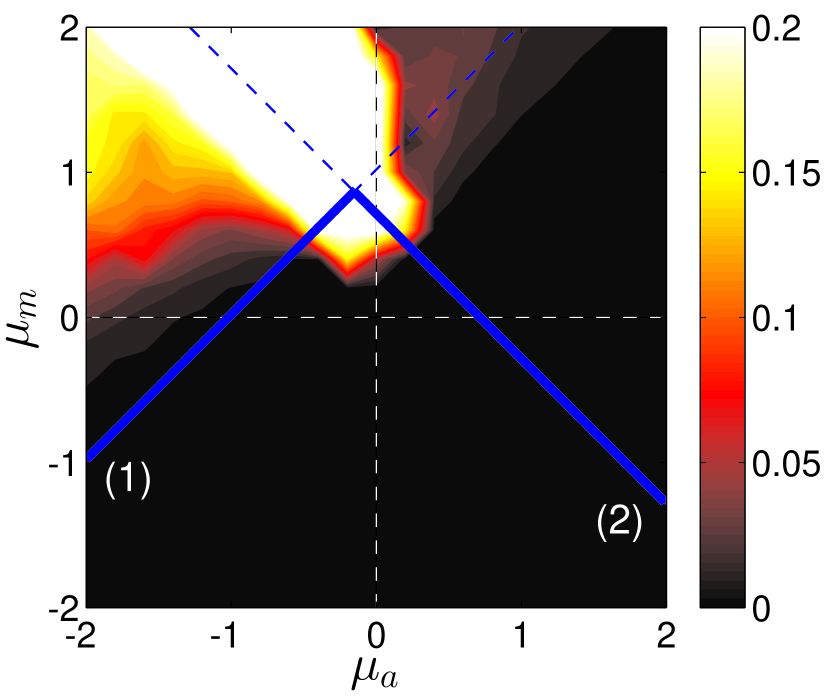
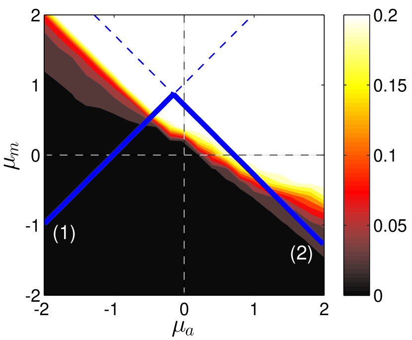
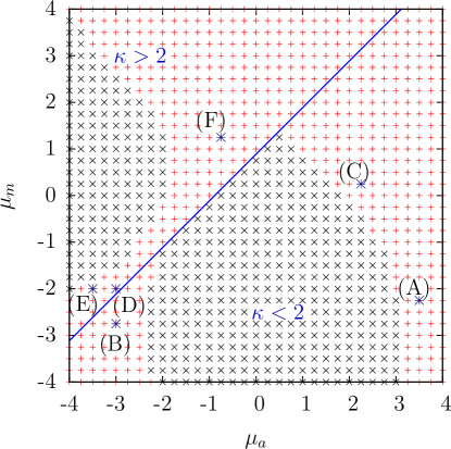
The illustrated method allows to explore the structure of the phase space of the dynamical system. In particular, we are interested in the stability of the solutions p(Φ)superscript𝑝Φp^{(\Phi)} in the (μm,μa)subscript𝜇𝑚subscript𝜇𝑎(\mu_{m},\mu_{a})-parameter space. For κ<2𝜅2\kappa<2, the stability of p(0)=ρ0/(2π)superscript𝑝0subscript𝜌02𝜋p^{(0)}=\rho_{0}/(2\pi) is investigated (Φ=0Φ0\Phi=0), whereas the solution p(Φ)(φ)superscript𝑝Φ𝜑p^{(\Phi)}(\varphi) (Φ>0Φ0\Phi>0) describing polar order is inserted in (2.1dz) for κ>2𝜅2\kappa>2. Figures 3 and 4 show the results of the stability analysis in the (μm,μa)subscript𝜇𝑚subscript𝜇𝑎(\mu_{m},\mu_{a})-parameter space and the dispersion relations for specific points (named (A)-(F) in figure 3 and figure 4), respectively.

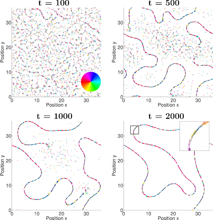
The kinetic approach reveals instabilities nearby the points (A) and (B). In these parameter regions, an interval of wavenumbers becomes unstable (cf. figure 4). In (A), nematic filaments are found in the individual based simulations (see section 5). However, a long-wavelength instability of the spatially homogeneous, disordered state p(0)superscript𝑝0p^{(0)} is found in (C). According to the individual based simulations, a clustering phase emerges nearby the point (C) (cf. figure 2E for a snapshot of a related simulation).

Close to the order-disorder transition line in the regime of collective motion (κ>2𝜅2\kappa>2), a long-wavelength instability emerges as can be seen in figure 4(D). According to figures 4(D)-(F), two hydrodynamic modes exist, which satisfy σ(k0)0bold-→𝜎bold-→k00\sigma(\bi{k}\rightarrow 0)\rightarrow 0, corresponding to transversal and longitudinal perturbations with respect to the direction of collective motion. The destabilization of the spatially homogeneous, ordered state p(Φ)superscript𝑝Φp^{(\Phi)} is always determined by these hydrodynamic modes, leading to long-wavelength instabilities.

Furthermore, there exists a region in the parameter space, where p(Φ)superscript𝑝Φp^{(\Phi)} is stable against spatially dependent perturbations. According to figure 3, this region is approximately bounded by the critical line κ=2𝜅2\kappa=2 (2.1do) and the secondary diagonal μm=μasubscript𝜇𝑚subscript𝜇𝑎\mu_{m}=-\mu_{a}, which is equally confirmed by the individual based simulation (see section 5).

In summary, it can be stated that the kinetic approach enables the prediction of the structure of the phase space as well as the dispersion relation for any microscopic model parameters. However, the analysis involves numerical methods. Unfortunately, it is not possible to deduce further analytical criteria for the stability of the solutions considered. For that purpose, additional assumptions are necessary, namely the restriction to the lowest Fourier coefficients and small wavenumbers, as shown in section 4. The hydrodynamic theory supplies analytical criteria for the stability of the solutions considered, such as critical microscopic model parameters.
Refer to caption
Figure 3: Stability of the solutions p(Φ)superscript𝑝Φp^{(\Phi)} in the (μm,μa)subscript𝜇𝑚subscript𝜇𝑎(\mu_{m},\mu_{a})-parameter space as predicted by the kinetic theory (truncation of (2.1dz) at n~=50~𝑛50\tilde{n}=50): black crosses indicate stable solutions, red plus signs indicate instabilities. The blue (solid) line corresponds to the critical line κ=2𝜅2\kappa=2 (2.1do). Collective motion is possible for κ>2𝜅2\kappa>2. The dispersion relation for the specific points (A)-(F) is given in figure 4. Whereas an interval of wavenumbers becomes unstable in (A) and (B), long-wavelength instabilities are found in (C)-(F). Parameters: Dφ=0.5subscript𝐷𝜑0.5D_{\varphi}=0.5; ρ0=1.5subscript𝜌01.5\rho_{0}=1.5; lc=0.2subscript𝑙𝑐0.2l_{c}=0.2; ls=1subscript𝑙𝑠1l_{s}=1; s0=1subscript𝑠01s_{0}=1; μr=1subscript𝜇𝑟1\mu_{r}=1; μasubscript𝜇𝑎\mu_{a} and μmsubscript𝜇𝑚\mu_{m} piecewise constant.
Refer to caption
Refer to caption
Refer to caption
Refer to caption
Refer to caption
Refer to caption
Figure 4: Dispersion relation σ(k=(k,0))𝜎kk0\sigma(\bi{k}=(k,0)) for specific points indicated in figure 3. Whereas an interval of wavenumbers becomes unstable in (A) and (B), long-wavelength instabilities are found in (C)-(F). Parameters: (A) μa=3.5subscript𝜇𝑎3.5\mu_{a}=3.5, μm=2.25subscript𝜇𝑚2.25\mu_{m}=-2.25; (B) μa=3subscript𝜇𝑎3\mu_{a}=-3, μm=2.75subscript𝜇𝑚2.75\mu_{m}=-2.75; (C) μa=2.25subscript𝜇𝑎2.25\mu_{a}=2.25, μm=0.25subscript𝜇𝑚0.25\mu_{m}=0.25; (D) μa=3subscript𝜇𝑎3\mu_{a}=-3, μm=2subscript𝜇𝑚2\mu_{m}=-2; (E) μa=3.5subscript𝜇𝑎3.5\mu_{a}=-3.5, μm=2subscript𝜇𝑚2\mu_{m}=-2; (F) μa=0.75subscript𝜇𝑎0.75\mu_{a}=-0.75, μm=1.25subscript𝜇𝑚1.25\mu_{m}=1.25. Other parameters: Dφ=0.5subscript𝐷𝜑0.5D_{\varphi}=0.5; ρ0=1.5subscript𝜌01.5\rho_{0}=1.5; lc=0.2subscript𝑙𝑐0.2l_{c}=0.2; ls=1subscript𝑙𝑠1l_{s}=1; s0=1subscript𝑠01s_{0}=1; μr=1subscript𝜇𝑟1\mu_{r}=1; μasubscript𝜇𝑎\mu_{a} and μmsubscript𝜇𝑚\mu_{m} piecewise constant.

In this context, we would like to emphasize one difficulty which occurs if the focus is put on the dynamics of the lowest Fourier coefficients on large length scales, i.e. small wavenumbers k𝑘k: The matrix elements K~n,r(k)subscript~𝐾𝑛𝑟k\tilde{K}_{n,r}(\bi{k}) involve Bessel functions of the first kind of k𝑘k (see B and [29]), which are oscillating functions with alternating Taylor coefficients [30]. The approximation

Jν,N(kx)m=0N(1)mm!Γ(m+ν+1)(kx2)2m+νsubscript𝐽𝜈𝑁𝑘𝑥superscriptsubscript𝑚0𝑁superscript1𝑚𝑚Γ𝑚𝜈1superscript𝑘𝑥22𝑚𝜈\displaystyle J_{\nu,N}(kx)\approx\sum_{m=0}^{N}\frac{(-1)^{m}}{m!\,\Gamma(m+\nu+1)}{\left(\frac{kx}{2}\right)}^{2m+\nu} (2.1dab)

will only be valid in the vicinity of k=0𝑘0k=0. For large k𝑘k, Jν,N(kx)subscript𝐽𝜈𝑁𝑘𝑥J_{\nu,N}(kx) tends to either plus or minus infinity, but never to zero. This issue will be important for the derivation of hydrodynamic equations in the next section and is restricting their validity to small wavenumbers k𝑘k and large length scales, respectively.

4 Derivation of Hydrodynamic Equations

4.1 Expansion of the Fokker-Planck Equation in the Angular Fourier Domain

In this section, a hydrodynamic description of the many-particle system is derived directly from the one-particle FPE (2.1dh). For this purpose, it is convenient to work in Fourier space with respect to the angular variable φ𝜑\varphi. Both, the particle density p(r,𝝋,t)𝑝r𝝋tp(\bi{r},\varphi,t) and the force Fφ(r,𝝋,t)subscript𝐹𝜑r𝝋tF_{\varphi}(\bi{r},\varphi,t) (2.1dg) are 2π2𝜋2\pi-periodic functions in φ𝜑\varphi. Hence, they can be expanded in a Fourier series as follows:

p(r,𝝋,t)𝑝r𝝋t\displaystyle p(\bi{r},\varphi,t) =12πn=f^n(r,t)ein𝝋,absent12𝜋superscriptsubscript𝑛subscript^𝑓𝑛rtsuperscriptein𝝋,\displaystyle=\frac{1}{2\pi}\sum_{n=-\infty}^{\infty}{\hat{f}}_{n}(\bi{r},t)\,e^{-in\varphi}\,\mbox{, } (2.1daa)
Fφ(r,𝝋,t)subscript𝐹𝜑r𝝋t\displaystyle F_{\varphi}(\bi{r},\varphi,t) =12πn=Q^n(r,t)ein𝝋.absent12𝜋superscriptsubscript𝑛subscript^𝑄𝑛rtsuperscriptein𝝋.\displaystyle=\frac{1}{2\pi}\sum_{n=-\infty}^{\infty}{\hat{Q}}_{n}(\bi{r},t)\,e^{-in\varphi}\,\mbox{. } (2.1dab)

The Fokker-Planck equation in Fourier space is obtained by multiplying (2.1dh) with einφsuperscript𝑒𝑖𝑛𝜑e^{in\varphi} and integration over φ[0,2π]𝜑02𝜋\varphi\in\left[0,2\pi\right]:

f^nt+s0(~f^n1+~f^n+1)=12πins0j=f^jQ^njn2Dφs02f^n.subscript^𝑓𝑛𝑡subscript𝑠0~subscript^𝑓𝑛1superscript~subscript^𝑓𝑛112𝜋𝑖𝑛subscript𝑠0superscriptsubscript𝑗subscript^𝑓𝑗subscript^𝑄𝑛𝑗superscript𝑛2subscript𝐷𝜑superscriptsubscript𝑠02subscript^𝑓𝑛.\displaystyle\frac{\partial{\hat{f}}_{n}}{\partial t}+s_{0}\left(\utilde{\nabla}{\hat{f}}_{n-1}+\utilde{\nabla}^{*}{\hat{f}}_{n+1}\right)=\frac{1}{2\pi}\frac{in}{s_{0}}\sum_{j=-\infty}^{\infty}{\hat{f}}_{j}\,{\hat{Q}}_{n-j}-n^{2}\frac{D_{\varphi}}{s_{0}^{2}}{\hat{f}}_{n}\,\mbox{. } (2.1dab)

In (2.1dab), the complex derivative ~=0.5(x+iy)~0.5subscript𝑥𝑖subscript𝑦\utilde{\nabla}=0.5\left(\partial_{x}+i\partial_{y}\right) was introduced. The Fourier coefficients

f^n(r,t)=02𝝅𝝋p(r,𝝋,t)ein𝝋=𝝆(r,t)ein𝝋subscript^𝑓𝑛rtsuperscriptsubscript02𝝅differential-d𝝋pr𝝋tsuperscriptein𝝋𝝆rtdelimited-⟨⟩superscriptein𝝋\displaystyle{\hat{f}}_{n}(\bi{r},t)=\int_{0}^{2\pi}\rmd\varphi\,p(\bi{r},\varphi,t)e^{in\varphi}=\rho(\bi{r},t)\left<e^{in\varphi}\right> (2.1dac)

obey the symmetry f^n(r,t)=f^n(r,t)superscriptsubscript^𝑓𝑛rtsubscriptbold-^fnrt{\hat{f}}_{n}^{*}(\bi{r},t)={\hat{f}}_{-n}(\bi{r},t), since p(r,𝝋,t)𝑝r𝝋tp(\bi{r},\varphi,t) is real-valued. The lowest Fourier coefficients are related to macroscopic physical quantities, namely the marginal particle density ρ(r,t)𝜌rt\rho(\bi{r},t) and also the momentum field w(r,t)=(wx,wy)wrtsubscriptwxsubscriptwy\bi{w}(\bi{r},t)=(w_{x},w_{y}) via

ρ(r,t)𝜌rt\displaystyle\rho(\bi{r},t) =f^0(r,t),absentsubscript^𝑓0rt\displaystyle={\hat{f}}_{0}(\bi{r},t)\,, (2.1dada)
wx(r,t)subscript𝑤𝑥rt\displaystyle w_{x}(\bi{r},t) =s02(f^1(r,t)+f^1(r,t)),absentsubscript𝑠02subscript^𝑓1rtsubscriptbold-^f1rt\displaystyle=\frac{s_{0}}{2}\left({\hat{f}}_{1}(\bi{r},t)+{\hat{f}}_{-1}(\bi{r},t)\right)\,, (2.1dadb)
wy(r,t)subscript𝑤𝑦rt\displaystyle w_{y}(\bi{r},t) =s02i(f^1(r,t)f^1(r,t)).absentsubscript𝑠02𝑖subscript^𝑓1rtsubscriptbold-^f1rt\displaystyle=\frac{s_{0}}{2i}\left({\hat{f}}_{1}(\bi{r},t)-{\hat{f}}_{-1}(\bi{r},t)\right)\,. (2.1dadc)

The second Fourier coefficients are related to the nematic order parameter |e2iφ|delimited-⟨⟩superscript𝑒2𝑖𝜑\left|\left<e^{2i\varphi}\right>\right| and the symmetric temperature tensor, as defined in [25, 23, 28], which is a measure for the width of the velocity distribution (see D for details). The dynamics of the temperature tensor is not derived explicitly in this context.

In the following, the dynamics of the density and the momentum field is deduced from (2.1dab). Therefore, the Fourier coefficients of the force Q^n(r,t)subscript^𝑄𝑛rt{\hat{Q}}_{n}(\bi{r},t) are approximatively calculated by expanding p(r+rji,𝝋,t)𝑝rsubscriptrji𝝋tp(\bi{r}+\bi{r}_{ji},\varphi,t) into a multidimensional Taylor series for small |rji|subscriptrji\left|\bi{r}_{ji}\right| [31], substituting (2.1daa) into (2.1dg) and evaluating the remaining integral. Here, we consider all terms up to the second order of the Taylor expansion. This approximation holds for spatially slowly varying densities, i.e. large system size compared to the interaction radius lssubscript𝑙𝑠l_{s}.

Again, the Fokker-Planck equation turns into an infinite hierarchy of equations (2.1dab) in Fourier space. An appropriate closure scheme is used in order to consider only the first Fourier coefficients. Close to the order-disorder transition, the degree of polar order is assumed to be small, i.e. |w|/(s0ρ)ϵproportional-towsubscript𝑠0𝜌italic-ϵ\left|\bi{w}\right|/(s_{0}\rho)\propto\epsilon, where ϵitalic-ϵ\epsilon is a small number and the particle density is locally close to the homogeneous distribution. Furthermore, the dynamics of the Fourier coefficients (2.1dab) suggests, that |f^1|subscript^𝑓1\left|{\hat{f}}_{1}\right| is larger than |f^n|subscript^𝑓𝑛\left|{\hat{f}}_{n}\right| with |n|>1𝑛1\left|n\right|>1, because of the damping term in (2.1dab) proportional to n2superscript𝑛2n^{2}, leading to the scaling relations

ρ(r,t)𝝆0ϵ,~ϵ,tϵ,f^nϵ|n|.formulae-sequenceproportional-to𝜌rtsubscript𝝆0bold-italic-ϵformulae-sequenceproportional-tobold-~bold-∇bold-italic-ϵformulae-sequenceproportional-tosubscripttbold-italic-ϵproportional-tosubscriptbold-^fnsuperscriptbold-italic-ϵn\displaystyle\rho(\bi{r},t)-\rho_{0}\propto\epsilon\,,\quad\utilde{\nabla}\propto\epsilon\,,\quad\partial_{t}\propto\epsilon\,,\quad{\hat{f}}_{n}\propto\epsilon^{\left|n\right|}\,. (2.1dade)

In [20] it is argued, that the scaling ansatz of the temporal and spatial derivatives reflects the propagating nature of the system. This closure scheme described above was already used in [17, 20, 31, 22] and in [21] in a modified way for nematic particles. A system of three nonlinear partial differential equations is obtained by keeping all terms up to the order ϵ3superscriptitalic-ϵ3\epsilon^{3}.

ρt𝜌𝑡\displaystyle\frac{\partial\rho}{\partial t} =s0(~f^1+~f^1)absentsubscript𝑠0~superscriptsubscript^𝑓1superscript~subscript^𝑓1\displaystyle=-s_{0}\left(\utilde{\nabla}{\hat{f}}_{1}^{*}+\utilde{\nabla}^{*}{\hat{f}}_{1}\right) (2.1dadfa)
f^1tsubscript^𝑓1𝑡\displaystyle\frac{\partial{\hat{f}}_{1}}{\partial t} =(ξ1ρξ5)f^1ξ1f^2f^1+(3245ξ3ρs0)~f^2+(329ξ3ρξ2ρs0)~ρabsentsubscript𝜉1𝜌subscript𝜉5subscript^𝑓1subscript𝜉1subscript^𝑓2superscriptsubscript^𝑓13245subscript𝜉3𝜌subscript𝑠0superscript~subscript^𝑓2329subscript𝜉3𝜌subscript𝜉2𝜌subscript𝑠0~𝜌\displaystyle=\left(\xi_{1}\rho-\xi_{5}\right){\hat{f}}_{1}-\xi_{1}{\hat{f}}_{2}{\hat{f}}_{1}^{*}+\left(\frac{32}{45}\xi_{3}\rho-s_{0}\right)\utilde{\nabla}^{*}{\hat{f}}_{2}+\left(\frac{32}{9}\xi_{3}\rho-\xi_{2}\rho-s_{0}\right)\utilde{\nabla}\rho (2.1dadfb)
6445ξ3f^1~f^1+ξ4ρ2(Δf^1+2~2f^1)6445subscript𝜉3superscriptsubscript^𝑓1~subscript^𝑓1subscript𝜉4𝜌2Δsubscript^𝑓12superscript~2superscriptsubscript^𝑓1\displaystyle\quad-\frac{64}{45}\xi_{3}{\hat{f}}_{1}^{*}\utilde{\nabla}{\hat{f}}_{1}+\frac{\xi_{4}\rho}{2}\left(\Delta{\hat{f}}_{1}+2\utilde{\nabla}^{2}{\hat{f}}_{1}^{*}\right)
f^2tsubscript^𝑓2𝑡\displaystyle\frac{\partial{\hat{f}}_{2}}{\partial t} =2[2ξ5f^2+ξ1f^12(s02+6445ξ3ρ)~f^1+(329ξ3ξ2)f^1~ρξ4ρ~2ρ]absent2delimited-[]2subscript𝜉5subscript^𝑓2subscript𝜉1superscriptsubscript^𝑓12subscript𝑠026445subscript𝜉3𝜌~subscript^𝑓1329subscript𝜉3subscript𝜉2subscript^𝑓1~𝜌subscript𝜉4𝜌superscript~2𝜌\displaystyle=2\left[-2\xi_{5}{\hat{f}}_{2}+\xi_{1}{\hat{f}}_{1}^{2}-\left(\frac{s_{0}}{2}+\frac{64}{45}\xi_{3}\rho\right)\utilde{\nabla}{\hat{f}}_{1}+\left(\frac{32}{9}\xi_{3}-\xi_{2}\right){\hat{f}}_{1}\utilde{\nabla}\rho-\xi_{4}\rho\utilde{\nabla}^{2}\rho\right] (2.1dadfc)

The following coefficients are introduced:

ξ1=subscript𝜉1absent\displaystyle\xi_{1}= π4lclsrjirji[μm(rji)μa(rji)],𝜋4superscriptsubscriptsubscript𝑙𝑐subscript𝑙𝑠differential-dsubscript𝑟𝑗𝑖subscript𝑟𝑗𝑖delimited-[]subscript𝜇𝑚subscript𝑟𝑗𝑖subscript𝜇𝑎subscript𝑟𝑗𝑖\displaystyle\frac{\pi}{4}\int_{l_{c}}^{l_{s}}\rmd r_{ji}\,r_{ji}\left[\mu_{m}(r_{ji})-\mu_{a}(r_{ji})\right]\,, (2.1dadfga)
ξ2=subscript𝜉2absent\displaystyle\xi_{2}= πs00lcrjirji2μr(rji),𝜋subscript𝑠0superscriptsubscript0subscript𝑙𝑐differential-dsubscript𝑟𝑗𝑖superscriptsubscript𝑟𝑗𝑖2subscript𝜇𝑟subscript𝑟𝑗𝑖\displaystyle\frac{\pi}{s_{0}}\int_{0}^{l_{c}}\rmd r_{ji}\,r_{ji}^{2}\,\mu_{r}(r_{ji})\,, (2.1dadfgb)
ξ3=subscript𝜉3absent\displaystyle\xi_{3}= 1πlclsrjirji2[μm(rji)+μa(rji)],1𝜋superscriptsubscriptsubscript𝑙𝑐subscript𝑙𝑠differential-dsubscript𝑟𝑗𝑖superscriptsubscript𝑟𝑗𝑖2delimited-[]subscript𝜇𝑚subscript𝑟𝑗𝑖subscript𝜇𝑎subscript𝑟𝑗𝑖\displaystyle\frac{1}{\pi}\int_{l_{c}}^{l_{s}}\rmd r_{ji}\,r_{ji}^{2}\left[\mu_{m}(r_{ji})+\mu_{a}(r_{ji})\right]\,, (2.1dadfgc)
ξ4=subscript𝜉4absent\displaystyle\xi_{4}= π8lclsrjirji3[μm(rji)μa(rji)],𝜋8superscriptsubscriptsubscript𝑙𝑐subscript𝑙𝑠differential-dsubscript𝑟𝑗𝑖superscriptsubscript𝑟𝑗𝑖3delimited-[]subscript𝜇𝑚subscript𝑟𝑗𝑖subscript𝜇𝑎subscript𝑟𝑗𝑖\displaystyle\frac{\pi}{8}\int_{l_{c}}^{l_{s}}\rmd r_{ji}\,r_{ji}^{3}\left[\mu_{m}(r_{ji})-\mu_{a}(r_{ji})\right]\,, (2.1dadfgd)
ξ5=subscript𝜉5absent\displaystyle\xi_{5}= Dφs02.subscript𝐷𝜑superscriptsubscript𝑠02\displaystyle\frac{D_{\varphi}}{s_{0}^{2}}\,. (2.1dadfge)

Equation (2.1dadfa) is simply the continuity equation representing the conservation of the particle number N𝑁N.

4.2 Hydrodynamic Limit

Another simplification of the system (4.1) is reached by adiabatically eliminating f^2subscript^𝑓2{\hat{f}}_{2}, i.e. tf^20subscript𝑡subscript^𝑓20\partial_{t}{\hat{f}}_{2}\approx 0, where

f^212ξ5[ξ1f^12(s02+6445ξ3ρ)~f^1]subscript^𝑓212subscript𝜉5delimited-[]subscript𝜉1superscriptsubscript^𝑓12subscript𝑠026445subscript𝜉3𝜌~subscript^𝑓1\displaystyle{\hat{f}}_{2}\approx\frac{1}{2\xi_{5}}\left[\xi_{1}{\hat{f}}_{1}^{2}-\left(\frac{s_{0}}{2}+\frac{64}{45}\xi_{3}\rho\right)\utilde{\nabla}{\hat{f}}_{1}\right] (2.1dadfgh)

follows. This approximation is only valid if the first Fourier mode relaxes considerably slower than f^2subscript^𝑓2{\hat{f}}_{2}. The assumption of a time scale separation between the first and second Fourier mode can be only be justified if |ξ1ρξ5|4ξ5much-less-thansubscript𝜉1𝜌subscript𝜉54subscript𝜉5\left|\xi_{1}\rho-\xi_{5}\right|\ll 4\xi_{5}, which is equivalent to 6κ10much-less-than6𝜅much-less-than10-6\ll\kappa\ll 10. Furthermore ξ5Dφ>0proportional-tosubscript𝜉5subscript𝐷𝜑0\xi_{5}\propto D_{\varphi}>0 has to hold.

Please note, that all terms of the order ϵ3superscriptitalic-ϵ3\epsilon^{3} were dropped in (2.1dadfgh) according to the scaling relations (2.1dade).

By identifying Fourier coefficients with physical quantities (4.1), familiar hydrodynamic equations are obtained.

ρt𝜌𝑡\displaystyle\frac{\partial\rho}{\partial t} =wabsentw\displaystyle=-\nabla\cdot\bi{w} (2.1dadfgia)
wtw𝑡\displaystyle\frac{\partial\bi{w}}{\partial t} =(λ1η1|w|2)w+𝝀2𝝆+𝝀4Δw+𝝀5(w)+𝜼2(w)wabsentsubscript𝜆1subscript𝜂1superscriptw2wsubscript𝝀2bold-∇𝝆subscript𝝀4Δwsubscript𝝀5bold-∇bold-⋅bold-∇wsubscript𝜼2bold-⋅wbold-∇w\displaystyle=\left(\lambda_{1}-\eta_{1}\left|\bi{w}\right|^{2}\right)\bi{w}+\lambda_{2}\nabla\rho+\lambda_{4}\,\Delta\bi{w}+\lambda_{5}\nabla(\nabla\cdot\bi{w})+\eta_{2}(\bi{w}\cdot\nabla)\,\bi{w} (2.1dadfgib)
+η3(12|w|2w(w))subscript𝜂312superscriptw2wbold-⋅bold-∇w\displaystyle\quad+\eta_{3}\left(\frac{1}{2}\nabla\left|\bi{w}\right|^{2}-\bi{w}\,(\nabla\cdot\bi{w})\right)

The transport coefficients {λi,ηi}subscript𝜆𝑖subscript𝜂𝑖\{\lambda_{i},\eta_{i}\} as functions of ξisubscript𝜉𝑖\xi_{i} (2.1dadf) read

λ1subscript𝜆1\displaystyle\lambda_{1} =ξ1ρξ5,absentsubscript𝜉1𝜌subscript𝜉5\displaystyle=\xi_{1}\rho-\xi_{5}, (2.1dadfgija)
λ2subscript𝜆2\displaystyle\lambda_{2} =s02(329ξ3ρξ2ρs0),absentsubscript𝑠02329subscript𝜉3𝜌subscript𝜉2𝜌subscript𝑠0\displaystyle=\frac{s_{0}}{2}\left(\frac{32}{9}\xi_{3}\rho-\xi_{2}\rho-s_{0}\right), (2.1dadfgijb)
λ4subscript𝜆4\displaystyle\lambda_{4} =14[s03245ξ3ρ2ξ5(s02+6445ξ3ρ)+ξ4ρ],absent14delimited-[]subscript𝑠03245subscript𝜉3𝜌2subscript𝜉5subscript𝑠026445subscript𝜉3𝜌subscript𝜉4𝜌\displaystyle=\frac{1}{4}\left[\frac{s_{0}-\frac{32}{45}\xi_{3}\rho}{2\xi_{5}}\left(\frac{s_{0}}{2}+\frac{64}{45}\xi_{3}\rho\right)+\xi_{4}\rho\right], (2.1dadfgijc)
λ5subscript𝜆5\displaystyle\lambda_{5} =ξ4ρ2,absentsubscript𝜉4𝜌2\displaystyle=\frac{\xi_{4}\rho}{2}, (2.1dadfgijd)
η1subscript𝜂1\displaystyle\eta_{1} =ξ122ξ5s02,absentsuperscriptsubscript𝜉122subscript𝜉5superscriptsubscript𝑠02\displaystyle=\frac{\xi_{1}^{2}}{2\xi_{5}s_{0}^{2}}, (2.1dadfgije)
η2subscript𝜂2\displaystyle\eta_{2} =3ξ18s0ξ5(256ξ3ρ135s0)32ξ345s0,absent3subscript𝜉18subscript𝑠0subscript𝜉5256subscript𝜉3𝜌135subscript𝑠032subscript𝜉345subscript𝑠0\displaystyle=\frac{3\xi_{1}}{8s_{0}\xi_{5}}\left(\frac{256\xi_{3}\rho}{135}-s_{0}\right)-\frac{32\xi_{3}}{45s_{0}}, (2.1dadfgijf)
η3subscript𝜂3\displaystyle\eta_{3} =5ξ18ξ532ξ345s0.absent5subscript𝜉18subscript𝜉532subscript𝜉345subscript𝑠0\displaystyle=\frac{5\xi_{1}}{8\xi_{5}}-\frac{32\xi_{3}}{45s_{0}}\ . (2.1dadfgijg)

The hydrodynamic equations (4.2) are comparable in structure to the theory of Toner and Tu [13, 14].

In the theory of Toner and Tu, the coefficients η2subscript𝜂2\eta_{2} and η3subscript𝜂3\eta_{3} are assumed to be nonzero phenomenological parameters due to the absence of Galilean invariance [14]. Indeed, in our model, η2subscript𝜂2\eta_{2} and η3subscript𝜂3\eta_{3} can take both, negative and positive values. Likewise, λ2subscript𝜆2\lambda_{2} can be positive and negative: A positive λ2subscript𝜆2\lambda_{2}-term leads to a flow into the direction of higher densities and consequently to clustering, as shown below. The damping coefficient η1subscript𝜂1\eta_{1} is positive for all microscopic parameters, consistently. The sign of the different transport coefficients is discussed in C in detail.

The stability of the hydrodynamic equations (4.2) requires that λ4subscript𝜆4\lambda_{4} and λ5subscript𝜆5\lambda_{5} are greater than zero. In this region, the hydrodynamic equations describe collectively moving bands and the theory of Toner and Tu applies. In contrast to the original Vicsek model, in our model the coefficients λ4subscript𝜆4\lambda_{4} and λ5subscript𝜆5\lambda_{5} may change signs. As shown in [3], a negative λ4subscript𝜆4\lambda_{4} may lead to an instability of spatially homogeneous states. In this case, higher order derivatives are needed in (2.1dadfgib) in order to guarantee the stability of the dynamics666The derivation of those terms goes beyond the scope of the present work. . Moreover, the time scale seperation of the first and second Fourier mode is only justified for ξ1ρξ5subscript𝜉1𝜌subscript𝜉5\xi_{1}\rho\approx\xi_{5}, i.e. λ10subscript𝜆10\lambda_{1}\approx 0. For the remaining analysis of the hydrodynamic equations, we will assume the stability and validity of our hydrodynamic theory (4.2).

Let us begin the analysis of (4.2) by neglecting the spatial derivatives and analyzing the fixed points of

wt=(λ1η1|w|2)w.differential-dwdifferential-d𝑡subscript𝜆1subscript𝜂1superscriptw2w\displaystyle\frac{\rmd\bi{w}}{\rmd t}=\left(\lambda_{1}-\eta_{1}\left|\bi{w}\right|^{2}\right)\bi{w}\,. (2.1dadfgijk)

That is the standard symmetry-breaking term present in all models of collective motion [14, 18, 3, 19, 31, 22, 20]. Apparently, two spatially homogeneous solutions exist: First, w0=0subscriptw00\bi{w}_{0}=0 corresponding to a disordered phase and vanishing center of mass velocity. Second,

w1=𝝀1𝜼1e,subscriptw1subscript𝝀1subscript𝜼1e\displaystyle\bi{w}_{1}=\sqrt{\frac{\lambda_{1}}{\eta_{1}}}\,\bi{e}\,, (2.1dadfgijl)

where ee\bi{e} denotes an arbitrary unit vector reflecting the isotropy of the system. Without loss of generality we set e=exesubscripte𝑥{\bi e}={\bi e}_{x}. For λ1<0subscript𝜆10\lambda_{1}<0, only the fixed point w0subscriptw0\bi{w}_{0} exists and is stable against spatially homogeneous perturbations. For λ10subscript𝜆10\lambda_{1}\geq 0, w1subscriptw1\bi{w}_{1} is a second fixed point corresponding to an ordered phase with nonzero mean-speed (swarming phase).
Refer to caption
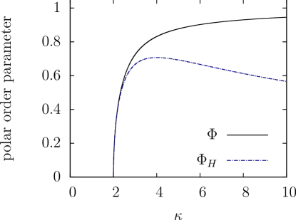
Figure 5: Comparison of the order parameter for the spatially homogeneous obtained as an exact solution of the nonlinear Fokker-Planck equation from (2.1dm) and the hydrodynamic theory (2.1dadfgijo).

The supercritical pitchfork bifurcation in λ1=0subscript𝜆10\lambda_{1}=0, i.e.

lclsrjirji(μm(rji)μa(rji))=4Dφπρ0s02,superscriptsubscriptsubscript𝑙𝑐subscript𝑙𝑠differential-dsubscript𝑟𝑗𝑖subscript𝑟𝑗𝑖subscript𝜇𝑚subscript𝑟𝑗𝑖subscript𝜇𝑎subscript𝑟𝑗𝑖4subscript𝐷𝜑𝜋subscript𝜌0superscriptsubscript𝑠02,\displaystyle\int_{l_{c}}^{l_{s}}\rmd r_{ji}\,r_{ji}\left(\mu_{m}(r_{ji})-\mu_{a}(r_{ji})\right)=\frac{4D_{\varphi}}{\pi\rho_{0}s_{0}^{2}}\,\mbox{, } (2.1dadfgijm)

corresponds to the order-disorder transition (2.1dp) described in section 3.1. By introducing the dimensionless coupling strength κ𝜅\kappa (2.1dj) again,

κ=πρ0s022Dφlclsrjirji(μm(rji)μa(rji)),𝜅𝜋subscript𝜌0superscriptsubscript𝑠022subscript𝐷𝜑superscriptsubscriptsubscript𝑙𝑐subscript𝑙𝑠differential-dsubscript𝑟𝑗𝑖subscript𝑟𝑗𝑖subscript𝜇𝑚subscript𝑟𝑗𝑖subscript𝜇𝑎subscript𝑟𝑗𝑖\displaystyle\kappa=\frac{\pi\rho_{0}s_{0}^{2}}{2D_{\varphi}}\int_{l_{c}}^{l_{s}}\rmd r_{ji}\,r_{ji}\left(\mu_{m}(r_{ji})-\mu_{a}(r_{ji})\right)\,, (2.1dadfgijn)

the polar order parameter ΦH=|w1|/(s0ρ0)subscriptΦ𝐻subscriptw1subscript𝑠0subscript𝜌0\Phi_{H}=\left|\bi{w}_{1}\right|/(s_{0}\rho_{0}) as described by the hydrodynamic theory can be written as follows777The density ρ(r,t)𝜌rt\rho(\bi{r},t) was approximated by ρ0subscript𝜌0\rho_{0} for that argument in accordance with (2.1dade). :

ΦH=2κ2κ.subscriptΦ𝐻2𝜅2𝜅\displaystyle\Phi_{H}=2\,\frac{\sqrt{\kappa-2}}{\kappa}\,. (2.1dadfgijo)

Close to the critical point κc=2subscript𝜅𝑐2\kappa_{c}=2, one recovers the correct scaling behaviour ΦHκ2similar-to-or-equalssubscriptΦ𝐻𝜅2\Phi_{H}\simeq\sqrt{\kappa-2} (2.1dp). However, for large κ𝜅\kappa the polar order parameter ΦHsubscriptΦ𝐻\Phi_{H} tends to zero according to (2.1dadfgijo) as shown in figure 5. This is a consequence of the approximations made, namely the elimination of higher Fourier modes. If one allows a maximal relative error (ΦΦH)/ΦΦsubscriptΦ𝐻Φ(\Phi-\Phi_{H})/\Phi of 5%percent55\%, an upper bound for κ𝜅\kappa is found numerically: κ2.617𝜅2.617\kappa\leq 2.617.

Equation (2.1dadfgijm) defines the transition line in the (μm(\mu_{m},μa)\mu_{a})-parameter space. Interestingly, only the integrated interaction strengths are important, the exact functional dependence on the distance between two particles μm,a=μm,a(rji)subscript𝜇𝑚𝑎subscript𝜇𝑚𝑎subscript𝑟𝑗𝑖\mu_{m,a}=\mu_{m,a}(r_{ji}) does not matter. Furthermore, collective motion is possible in both situations, pure attraction to particles moving away (μm>0subscript𝜇𝑚0\mu_{m}>0, μa=0subscript𝜇𝑎0\mu_{a}=0) and pure repulsion from approaching particles (μm=0subscript𝜇𝑚0\mu_{m}=0, μa<0subscript𝜇𝑎0\mu_{a}<0), respectively. Since the critical coupling parameter κc=2subscript𝜅𝑐2\kappa_{c}=2 is positive, polar order cannot be found in the anti-alignment regime.

4.3 Stability of the spatially homogeneous solutions

We proceed with the analysis of homogeneous solutions against spatial perturbations. At first, let us consider the stability of the disordered, homogeneous solution with w0=0subscriptw00\bi{w}_{0}=0. In order to investigate the stability of w0subscriptw0\bi{w}_{0}, the ansatz

ρ(r,t)𝜌rt\displaystyle\rho(\bi{r},t) =ρ0+δρ(r,t),absentsubscript𝜌0𝛿𝜌rt\displaystyle=\rho_{0}+\delta\rho(\bi{r},t)\,, (2.1dadfgijpa)
w(r,t)wrt\displaystyle\bi{w}(\bi{r},t) =δw(r,t)absent𝛿wrt\displaystyle=\delta\bi{w}(\bi{r},t)\, (2.1dadfgijpb)

is inserted in (4.2) and the resulting equations are linearized in the perturbations which are assumed to be small. The linearized equations read

δρt𝛿𝜌𝑡\displaystyle\frac{\partial\delta\rho}{\partial t} =δw,absent𝛿w\displaystyle=-\nabla\cdot\delta\bi{w}\,, (2.1dadfgijpqa)
δwt𝛿w𝑡\displaystyle\frac{\partial\delta\bi{w}}{\partial t} =λ1δw+𝝀2𝜹𝝆+𝝀4Δ𝜹w+𝝀5(𝜹w).absentsubscript𝜆1𝛿wsubscript𝝀2bold-∇𝜹𝝆subscript𝝀4Δ𝜹wsubscript𝝀5bold-∇bold-⋅bold-∇𝜹w\displaystyle=\lambda_{1}\delta\bi{w}+\lambda_{2}\nabla\delta\rho+\lambda_{4}\,\Delta\delta\bi{w}+\lambda_{5}\nabla(\nabla\cdot\delta\bi{w})\,. (2.1dadfgijpqb)

Inserting the exponential ansatz

δρ(r,t)𝛿𝜌rt\displaystyle\delta\rho(\bi{r},t) =ζρexp(σt+ikr),absentsubscript𝜁𝜌𝜎𝑡bold-⋅𝑖kr\displaystyle=\zeta_{\rho}\exp\left(\sigma t+i\bi{k}\cdot\bi{r}\right)\,, (2.1dadfgijpqra)
δw(r,t)𝛿wrt\displaystyle\delta\bi{w}(\bi{r},t) =𝜻wexp(σt+ikr)absentsubscript𝜻w𝜎𝑡bold-⋅𝑖kr\displaystyle=\boldsymbol{\zeta}_{\bi{w}}\exp\left(\sigma t+i\bi{k}\cdot\bi{r}\right) (2.1dadfgijpqrb)

yields the dispersion relation σ(k)𝜎k\sigma(\bi{k}). Since w0subscriptw0\bi{w}_{0} is isotropic, the eigenvalues σ𝜎\sigma are independent of the direction of the wavevector.

σ1subscript𝜎1\displaystyle\sigma_{1} =λ1λ4k2,absentsubscript𝜆1subscript𝜆4superscript𝑘2\displaystyle=\lambda_{1}-\lambda_{4}k^{2}\,, (2.1dadfgijpqrsa)
σ2,3subscript𝜎23\displaystyle\sigma_{2,3} =12[λ1(λ4+λ5)k2±[λ1(λ4+λ5)k2]2+4k2λ2].absent12delimited-[]plus-or-minussubscript𝜆1subscript𝜆4subscript𝜆5superscript𝑘2superscriptdelimited-[]subscript𝜆1subscript𝜆4subscript𝜆5superscript𝑘224superscript𝑘2subscript𝜆2\displaystyle=\frac{1}{2}\left[\lambda_{1}-\left(\lambda_{4}+\lambda_{5}\right)k^{2}\pm\sqrt{\left[\lambda_{1}-(\lambda_{4}+\lambda_{5})\,k^{2}\right]^{2}+4k^{2}\lambda_{2}}\,\right]\,. (2.1dadfgijpqrsb)

Provided all eigenvalues are less than zero, the disordered spatially homogeneous state is stable. The first eigenvalue σ1subscript𝜎1\sigma_{1} is equal to λ1subscript𝜆1\lambda_{1} for k=0𝑘0k=0, i.e. the stability of w0subscriptw0\bi{w}_{0} is determined by the sign of λ1subscript𝜆1\lambda_{1}. That is the destabilization of the homogeneous state as discussed before. For λ4>0subscript𝜆40\lambda_{4}>0, the first eigenvalue σ1subscript𝜎1\sigma_{1} is monotonically decreasing. However, the eigenvalue σ1subscript𝜎1\sigma_{1} is monotonically increasing for λ4<0subscript𝜆40\lambda_{4}<0. In this case, the hydrodynamic equations (4.2) loose their validity. This unphysical behaviour is due to the restriction to second derivatives when the integral (2.1dg) was calculated. Furthermore, it is problematically that the Taylor coefficients have alternating signs so that Taylor polynomials converge slowly as argued at the end of section 3.2. To predict the behaviour of the system in that case, one needs to consider higher order terms. Unfortunately, the number of terms and Fourier coefficients that has to be considered to be consistent with the scaling ansatz (2.1dade), grows rapidly.

Nevertheless, it is possible to predict the stability of w0subscriptw0\bi{w}_{0} by analyzing those eigenvalues, which tend to zero for small wavenumbers (hydrodynamic modes [14]). For small wavenumbers, the eigenvalue σ2subscript𝜎2\sigma_{2} (σ2>σ3subscript𝜎2subscript𝜎3\sigma_{2}>\sigma_{3}) is expanded in a Taylor series:

σ2λ2λ1k2+λ22λ1λ2(λ4+λ5)λ13k4+𝒪(k6).similar-to-or-equalssubscript𝜎2subscript𝜆2subscript𝜆1superscript𝑘2superscriptsubscript𝜆22subscript𝜆1subscript𝜆2subscript𝜆4subscript𝜆5superscriptsubscript𝜆13superscript𝑘4𝒪superscript𝑘6\displaystyle\sigma_{2}\simeq-\frac{\lambda_{2}}{\lambda_{1}}\,k^{2}+\frac{\lambda_{2}^{2}-\lambda_{1}\lambda_{2}\left(\lambda_{4}+\lambda_{5}\right)}{\lambda_{1}^{3}}\,k^{4}+\mathcal{O}(k^{6})\,. (2.1dadfgijpqrst)

Close to the order-disorder transition line, λ1subscript𝜆1\lambda_{1} is approximately zero. Therefore it is sufficient to keep the leading order terms in 1/λ11subscript𝜆11/\lambda_{1} [18]:

σ2λ2λ1k2+λ22λ13k4+𝒪(k6).similar-to-or-equalssubscript𝜎2subscript𝜆2subscript𝜆1superscript𝑘2superscriptsubscript𝜆22superscriptsubscript𝜆13superscript𝑘4𝒪superscript𝑘6\displaystyle\sigma_{2}\simeq-\frac{\lambda_{2}}{\lambda_{1}}\,k^{2}+\frac{\lambda_{2}^{2}}{\lambda_{1}^{3}}\,k^{4}+\mathcal{O}(k^{6})\,. (2.1dadfgijpqrsu)

Suppose, w0subscriptw0\bi{w}_{0} is stable against spatially homogeneous perturbations, i.e. λ1<0subscript𝜆10\lambda_{1}<0. In that case, a long-wavelength instability emerges for positive λ2subscript𝜆2\lambda_{2}. Considering (4.2), this instability is reasonable: for λ2>0subscript𝜆20\lambda_{2}>0, inhomogeneities in the particle density will lead to a flow in the direction of the density gradients while for λ2<0subscript𝜆20\lambda_{2}<0 density inhomogeneities decay due to inverse flows. The amplification of density gradients will lead to an agglomeration of particles (cf. figure 2E). This hypothesis is supported by numerical simulations of the microscopic model, as shown in the next section and in [28]. A similar instability due to the gradient term in (4.2) is also known from other active matter systems [22]. Whereas in [22] the instability is due to the density-dependent motility of the particles, in our case the instability is referable to the selective interaction. The critical line is given by λ2=0subscript𝜆20\lambda_{2}=0, i.e.

lclsdrjirji2(μm(rji)+μa(rji))=9π16s0ρ0(s022+ρ0π20lcrjirji2μr(rji)).superscriptsubscriptsubscript𝑙𝑐subscript𝑙𝑠dsubscript𝑟𝑗𝑖superscriptsubscript𝑟𝑗𝑖2subscript𝜇𝑚subscript𝑟𝑗𝑖subscript𝜇𝑎subscript𝑟𝑗𝑖9𝜋16subscript𝑠0subscript𝜌0superscriptsubscript𝑠022subscript𝜌0𝜋2superscriptsubscript0subscript𝑙𝑐differential-dsubscript𝑟𝑗𝑖superscriptsubscript𝑟𝑗𝑖2subscript𝜇𝑟subscript𝑟𝑗𝑖\displaystyle\int_{l_{c}}^{l_{s}}\mbox{d}r_{ji}\,r_{ji}^{2}\left(\mu_{m}(r_{ji})+\mu_{a}(r_{ji})\right)=\frac{9\pi}{16s_{0}\rho_{0}}\left(\frac{s_{0}^{2}}{2}+\frac{\rho_{0}\pi}{2}\int_{0}^{l_{c}}\rmd r_{ji}\,r_{ji}^{2}\mu_{r}(r_{ji})\right)\,. (2.1dadfgijpqrsv)

The corresponding analysis of the stability of the spatially homogeneous ordered state for |w1|>0subscriptw10|\bi{w}_{1}|>0 using the full hydrodynamic equations is much more complicated. It is done in great detail for the original Vicsek model in [18] for structurally identical hydrodynamic equations. In the following, the key points of the analysis are summarized. Moreover, an additional instability is found that is not present in the Vicsek model because in our model the transport coefficients λ2subscript𝜆2\lambda_{2}, η2subscript𝜂2\eta_{2} and η3subscript𝜂3\eta_{3} may change their algebraic signs. Inserting the ansatz

ρ(r,t)𝜌rt\displaystyle\rho(\bi{r},t) =ρ0+δρ(r,t),absentsubscript𝜌0𝛿𝜌rt\displaystyle=\rho_{0}+\delta\rho(\bi{r},t)\,, (2.1dadfgijpqrswa)
w(r,t)wrt\displaystyle\bi{w}(\bi{r},t) =w1+𝜹w(r,t)absentsubscriptw1𝜹wrt\displaystyle=\bi{w}_{1}+\delta\bi{w}(\bi{r},t)\, (2.1dadfgijpqrswb)

into (4.2) and linearization yields

δρt𝛿𝜌𝑡\displaystyle\frac{\partial\delta\rho}{\partial t} =δw,absent𝛿w\displaystyle=-\nabla\cdot\delta\bi{w}\,, (2.1dadfgijpqrswxa)
δwt𝛿w𝑡\displaystyle\frac{\partial\delta\bi{w}}{\partial t} =λ1ρ|ρ0δρw12𝜼1(w1𝜹w)w1+𝝀2𝜹𝝆+𝝀4Δ𝜹w+𝝀5(𝜹w)absentevaluated-atsubscript𝜆1𝜌subscript𝜌0𝛿𝜌subscriptw12subscript𝜼1bold-⋅subscriptw1𝜹wsubscriptw1subscript𝝀2bold-∇𝜹𝝆subscript𝝀4Δ𝜹wsubscript𝝀5bold-∇bold-⋅bold-∇𝜹w\displaystyle=\left.\frac{\partial\lambda_{1}}{\partial\rho}\right|_{\rho_{0}}\delta\rho\,\bi{w}_{1}-2\eta_{1}\left(\bi{w}_{1}\cdot\delta\bi{w}\right)\bi{w}_{1}+\lambda_{2}\nabla\delta\rho+\lambda_{4}\Delta\delta\bi{w}+\lambda_{5}\nabla(\nabla\cdot\delta\bi{w}) (2.1dadfgijpqrswxb)
+η2(w1)δw+𝜼3((w1𝜹w)w1(𝜹w)).subscript𝜂2bold-⋅subscriptw1bold-∇𝛿wsubscript𝜼3bold-∇bold-⋅subscriptw1𝜹wsubscriptw1bold-⋅bold-∇𝜹w\displaystyle\quad+\eta_{2}\left(\bi{w}_{1}\cdot\nabla\right)\delta\bi{w}+\eta_{3}\left(\nabla\left(\bi{w}_{1}\cdot\delta\bi{w}\right)-\bi{w}_{1}\left(\nabla\cdot\delta\bi{w}\right)\right)\,.

Again, inserting (2.1dadfgijpq) yields the growth rate σ𝜎\sigma dependent on the wavevector kk\bi{k}. We restrict ourselves to longitudinal perturbations, meaning that the wavevector kk\bi{k}, the perturbation δw𝛿w\delta\bi{w} and the direction of collective motion w0subscriptw0\bi{w}_{0} are pointing in the same direction, because we are interested in the emergence of collectively moving bands (cf. figure 2). The growth rate reads

σ±subscript𝜎plus-or-minus\displaystyle\sigma_{\pm} =12[2λ1(λ4+λ5)k2+iη2|w1|k±α1+iα2],absent12delimited-[]plus-or-minus2subscript𝜆1subscript𝜆4subscript𝜆5superscript𝑘2𝑖subscript𝜂2subscriptw1𝑘subscript𝛼1𝑖subscript𝛼2\displaystyle=\frac{1}{2}\left[-2\lambda_{1}-\left(\lambda_{4}+\lambda_{5}\right)k^{2}+i\eta_{2}\left|\bi{w}_{1}\right|k\pm\sqrt{\alpha_{1}+i\alpha_{2}}\,\right]\,, (2.1dadfgijpqrswxy)

where the coefficients

α1subscript𝛼1\displaystyle\alpha_{1} =[(λ4+λ5)k2+2λ1]2k2[(η2|w1|)24λ2],absentsuperscriptdelimited-[]subscript𝜆4subscript𝜆5superscript𝑘22subscript𝜆12superscript𝑘2delimited-[]superscriptsubscript𝜂2subscriptw124subscript𝜆2\displaystyle=\left[\left(\lambda_{4}+\lambda_{5}\right)k^{2}+2\lambda_{1}\right]^{2}-k^{2}\left[\left(\eta_{2}\left|\bi{w}_{1}\right|\right)^{2}-4\lambda_{2}\right]\,, (2.1dadfgijpqrswxza)
α2subscript𝛼2\displaystyle\alpha_{2} =2|w1|k{2λ1ρ|ρ0+η2[(λ4+λ5)k2+2λ1]}absent2subscriptw1𝑘evaluated-at2subscript𝜆1𝜌subscript𝜌0subscript𝜂2delimited-[]subscript𝜆4subscript𝜆5superscript𝑘22subscript𝜆1\displaystyle=-2\left|\bi{w}_{1}\right|k\left\{2\left.\frac{\partial\lambda_{1}}{\partial\rho}\right|_{\rho_{0}}+\eta_{2}\left[\left(\lambda_{4}+\lambda_{5}\right)k^{2}+2\lambda_{1}\right]\right\} (2.1dadfgijpqrswxzb)

were introduced. The real part of the largest eigenvalue reads as follows:

Re(σ+)(k2)Resubscript𝜎superscript𝑘2\displaystyle\mbox{Re}(\sigma_{+})(k^{2}) =λ1λ4+λ52k2+α1+α12+α228.absentsubscript𝜆1subscript𝜆4subscript𝜆52superscript𝑘2subscript𝛼1superscriptsubscript𝛼12superscriptsubscript𝛼228\displaystyle=-\lambda_{1}-\frac{\lambda_{4}+\lambda_{5}}{2}k^{2}+\sqrt{\frac{\alpha_{1}+\sqrt{\alpha_{1}^{2}+\alpha_{2}^{2}}}{8}}\,. (2.1dadfgijpqrswxzaa)

Close to the order-disorder transition, λ1subscript𝜆1\lambda_{1} is small, with the result that it is sufficient to keep the lowest order in 1/λ11subscript𝜆11/\lambda_{1}. The following expression is obtained for small wavenumbers [18]:

Re(σ+)(k2)=ξ128η1λ12k25ξ14128η12λ15k4+𝒪(k6).Resubscript𝜎superscript𝑘2superscriptsubscript𝜉128subscript𝜂1superscriptsubscript𝜆12superscript𝑘25superscriptsubscript𝜉14128superscriptsubscript𝜂12superscriptsubscript𝜆15superscript𝑘4𝒪superscript𝑘6\displaystyle\mbox{Re}(\sigma_{+})(k^{2})=\frac{\xi_{1}^{2}}{8\eta_{1}\lambda_{1}^{2}}k^{2}-\frac{5\xi_{1}^{4}}{128\eta_{1}^{2}\lambda_{1}^{5}}k^{4}+\mathcal{O}(k^{6})\,. (2.1dadfgijpqrswxzab)

That implies, that for λ10greater-than-or-equivalent-tosubscript𝜆10\lambda_{1}\gtrsim 0, a long-wavelength instability emerges. By expanding (2.1dadfgijpqrswxzaa) in a Taylor series for small k𝑘k (not assuming that λ10similar-to-or-equalssubscript𝜆10\lambda_{1}\simeq 0), one obtains

Re(σ+)(k2)=(1η1(ξ1λ1+η2)η22η1+4λ2λ1)k28+𝒪(k4).Resubscript𝜎superscript𝑘21subscript𝜂1subscript𝜉1subscript𝜆1subscript𝜂2superscriptsubscript𝜂22subscript𝜂14subscript𝜆2subscript𝜆1superscript𝑘28𝒪superscript𝑘4\displaystyle\mbox{Re}(\sigma_{+})(k^{2})=\left(\frac{1}{\eta_{1}}\left(\frac{\xi_{1}}{\lambda_{1}}+\eta_{2}\right)-\frac{\eta_{2}^{2}}{\eta_{1}}+\frac{4\lambda_{2}}{\lambda_{1}}\right)\frac{k^{2}}{8}+\mathcal{O}(k^{4})\,. (2.1dadfgijpqrswxzac)

In general, an instability appears, if the first Taylor coefficient becomes positive, because σ+(k0)0subscript𝜎𝑘00\sigma_{+}(k\rightarrow 0)\rightarrow 0. Unfortunately, it is not illuminating to derive the critical line μm=f(μa)subscript𝜇𝑚𝑓subscript𝜇𝑎\mu_{m}=f(\mu_{a}), where the relevant Taylor coefficient is zero, analytically, because the resulting expressions are quite complicated. The numerical analysis reveals that the spatially homogeneous, ordered state is unstable beyond a hyperbola which is bounded by the two asymptotes (see also figure 6)

μm+μa=135π64ρ0s0(ls3lc3)(s022+2πρ0lc3μr21),subscript𝜇𝑚subscript𝜇𝑎135𝜋64subscript𝜌0subscript𝑠0superscriptsubscript𝑙𝑠3superscriptsubscript𝑙𝑐3superscriptsubscript𝑠0222𝜋subscript𝜌0superscriptsubscript𝑙𝑐3subscript𝜇𝑟21\displaystyle\mu_{m}+\mu_{a}=\frac{135\pi}{64\rho_{0}s_{0}\left(l_{s}^{3}-l_{c}^{3}\right)}\left(\frac{s_{0}^{2}}{2}+\frac{2\pi\rho_{0}l_{c}^{3}\mu_{r}}{21}\right)\,, (2.1dadfgijpqrswxzada)
μmμa=8Dφπρ0s02(ls2lc2).subscript𝜇𝑚subscript𝜇𝑎8subscript𝐷𝜑𝜋subscript𝜌0superscriptsubscript𝑠02superscriptsubscript𝑙𝑠2superscriptsubscript𝑙𝑐2\displaystyle\mu_{m}-\mu_{a}=\frac{8D_{\varphi}}{\pi\rho_{0}s_{0}^{2}\left(l_{s}^{2}-l_{c}^{2}\right)}\,. (2.1dadfgijpqrswxzadb)

The instability of w1subscriptw1\bi{w}_{1} for

μm+μa>135π64ρ0s0(ls3lc3)(s022+2πρ0lc3μr21)subscript𝜇𝑚subscript𝜇𝑎135𝜋64subscript𝜌0subscript𝑠0superscriptsubscript𝑙𝑠3superscriptsubscript𝑙𝑐3superscriptsubscript𝑠0222𝜋subscript𝜌0superscriptsubscript𝑙𝑐3subscript𝜇𝑟21\displaystyle\mu_{m}+\mu_{a}>\frac{135\pi}{64\rho_{0}s_{0}\left(l_{s}^{3}-l_{c}^{3}\right)}\left(\frac{s_{0}^{2}}{2}+\frac{2\pi\rho_{0}l_{c}^{3}\mu_{r}}{21}\right) (2.1dadfgijpqrswxzadae)

is due to the selective interaction, therefore it is not present in the original Vicsek model. The two asymptotes (4.3) were derived using the approximation that the interaction strengths do not depend on the distance. The second line (2.1dadfgijpqrswxzadb) is equal to the critical line λ1=0subscript𝜆10\lambda_{1}=0 (2.1dadfgijm).

As already mentioned, negative values of λ4subscript𝜆4\lambda_{4} and λ5subscript𝜆5\lambda_{5} may lead to additional instabilities, which go beyond the scope of this work, because the hydrodynamic equations are restricted to second derivatives. However, neither (2.1dadfgijpqrsu), (2.1dadfgijpqrswxzab) nor (2.1dadfgijpqrswxzac) depend on λ4subscript𝜆4\lambda_{4} and λ5subscript𝜆5\lambda_{5}. Hence, the spatially homogeneous states and instabilities described above are always present in our model.
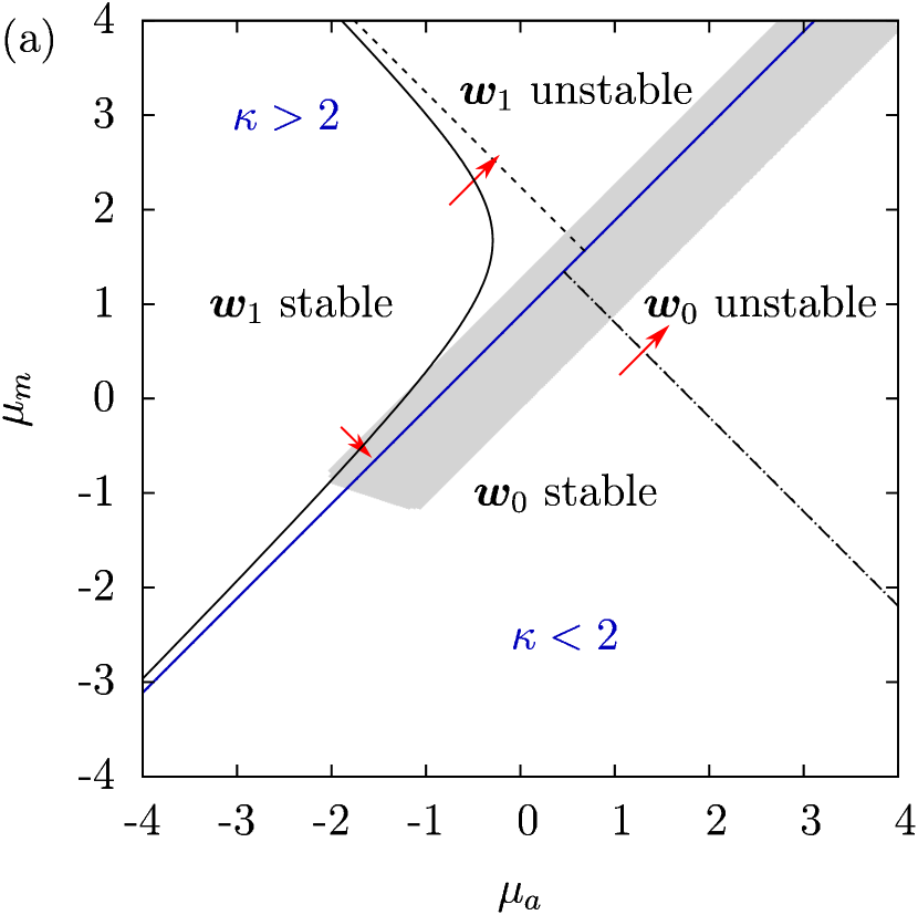
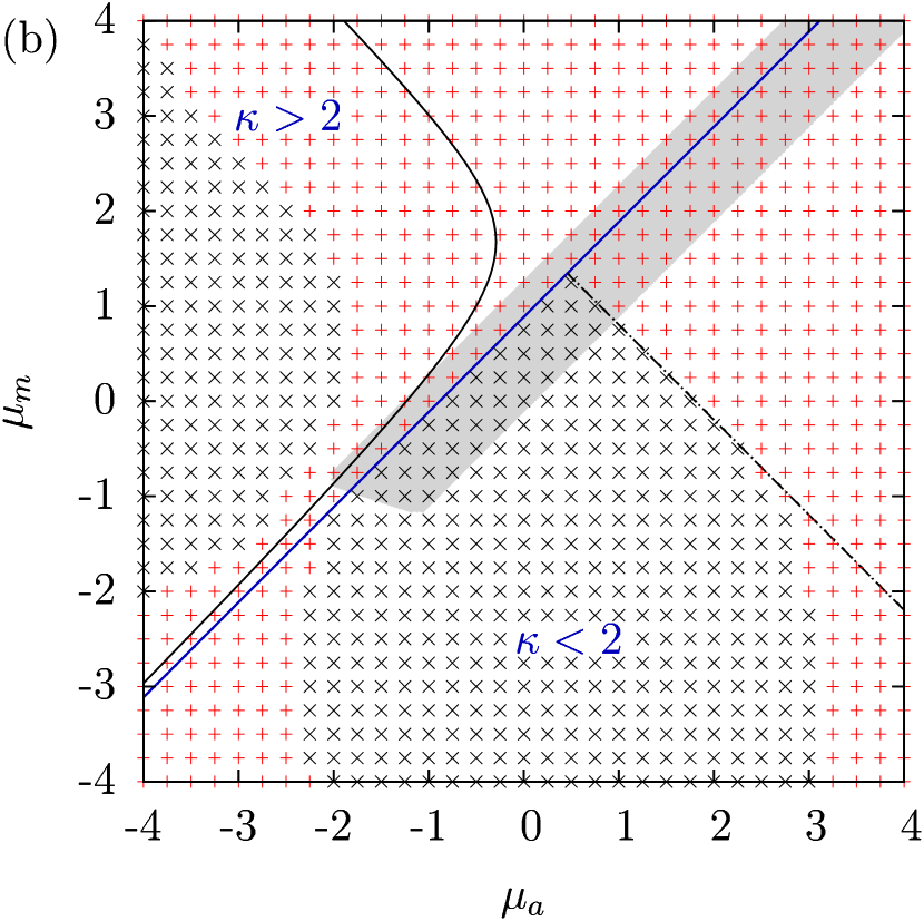
Refer to caption
Refer to caption
Figure 6: (a) Phase space as predicted by the hydrodynamic theory and (b) phase space in comparison to the predictions of the kinetic approach (see section 3.2). The arrows indicate long-wavelength instabilities in (a), black crosses indicate stable solutions, red plus signs indicate instabilities (see also figure 3) in figure (b). Below the critical blue (solid) line λ1=0subscript𝜆10\lambda_{1}=0 (equal to κ=2𝜅2\kappa=2 (2.1dadfgijm)), only the solution w0=0subscriptw00\bi{w}_{0}=0 (among the spatially homogeneous solutions) exists. It is unstable above the critical (dotdashed) line λ2=0subscript𝜆20\lambda_{2}=0 (2.1dadfgijpqrsv). Above the blue (solid) line, w0subscriptw0\bi{w}_{0} is unstable. Besides, the solution w1=𝝀1/𝜼1esubscriptw1subscript𝝀1subscript𝜼1e\bi{w}_{1}=\sqrt{\lambda_{1}/\eta_{1}}\,\bi{e} exists. It is unstable beyond a hyperbola that is bounded by two asymptotes according to the hydrodynamic theory: black (dashed) line (2.1dadfgijpqrswxzada) and blue (solid) line (2.1dadfgijpqrswxzadb). The subspace of the parameter space where the hydrodynamic theory is valid is indicated by the grey-shaded region. Parameters: Dφ=0.5subscript𝐷𝜑0.5D_{\varphi}=0.5; ρ0=1.5subscript𝜌01.5\rho_{0}=1.5; lc=0.2subscript𝑙𝑐0.2l_{c}=0.2; ls=1subscript𝑙𝑠1l_{s}=1; s0=1subscript𝑠01s_{0}=1; μr=1subscript𝜇𝑟1\mu_{r}=1; μasubscript𝜇𝑎\mu_{a} and μmsubscript𝜇𝑚\mu_{m} piecewise constant.

The predictions of the hydrodynamic theory, derived in this section, are compared to the predictions of the stability analysis using the kinetic description in section 3.2 in figure 6(b). The long-wavelength instability of w0subscriptw0\bi{w}_{0}, leading to clustering for λ2>0subscript𝜆20\lambda_{2}>0 as well as the long-wavelength instability close to the critical point (κ=2𝜅2\kappa=2, λ1=0subscript𝜆10\lambda_{1}=0) are confirmed by the kinetic approach.

Within the range of validity of the hydrodynamic theory, no contradictions are found with the kinetic theory. However, figure 6(b) indicates that the range of validity of the hydrodynamic theory does not cover all relevant parts of the parameter space. In particular, the destabilization of the ordered state w1subscriptw1\bi{w}_{1} is not sufficiently well described by the hydrodynamic equations. Please note, that the hydrodynamic theory is only valid for λ4>0subscript𝜆40\lambda_{4}>0 (guarantees the stability for large wavenumbers) and 0κ2.6170𝜅2.6170\leq\kappa\leq 2.617, where the lower bound is equivalent to λ5>0subscript𝜆50\lambda_{5}>0 and the upper bound ensures small deviations ΦΦHΦsubscriptΦ𝐻\Phi-\Phi_{H}. Due to the last limitation, it is impossible to study the dynamics of the system for high order parameters, i.e. far away from the critical point.

However, one can show numerically that the dispersion relations of the hydrodynamic theory (4.2) and the full system (3.2) coincide for small wavenumbers in the parameter range, where the hydrodynamic equations are valid. The hydrodynamic theory yields only three eigenvalues, which coincide with three eigenvalues given by the kinetic theory in the limit k0𝑘0k\rightarrow 0. For large k𝑘k, deviations occur due to the restriction to second derivatives (cf. scaling ansatz (2.1dade)).

Nevertheless, the hydrodynamic theory yields important insights on the macroscopic behaviour of the system. The symmetry breaking, i.e. the existence of a collective motion mode is predicted. Moreover, the stability of the homogeneous solutions to the hydrodynamic equations can be analyzed analytically and it allows to obtain analytical results on the order-disorder transition line as well as the occurrence of clustering. Thus, the structure of the phase space is roughly estimated by the hydrodynamic theory. New instabilities are found due to changes in the algebraic signs of the coefficients λ2subscript𝜆2\lambda_{2} and η2subscript𝜂2\eta_{2}. Furthermore, the structure of the theory suggests, that all predictions of the theory by Toner and Tu [14] are expected to arise in our system, such as giant number fluctuations. Within the range of validity of the hydrodynamic theory, the predictions of the kinetic theory, which is based on the mean-field assumption only (see section 3 for details), are in agreement with the hydrodynamic theory, whose range of validity is known quantitatively.

4.4 Large-System Limit

The hydrodynamic theory is simplified further, if the limit of large systems, i.e. large particle densities (N𝑁N\rightarrow\infty) and small interaction regions (ls0subscript𝑙𝑠0l_{s}\rightarrow 0) is considered, such that the number of particle within the interaction area is kept fixed: ρls2const𝜌superscriptsubscript𝑙𝑠2const\rho\,l_{s}^{2}\approx\mbox{const}. This approximation corresponds to a zeroth order Taylor expansion of the force (2.1dg): p(r+rji,𝝋j,t)p(r,𝝋j,t)𝑝rsubscriptrjisubscript𝝋jtprsubscript𝝋jtp(\bi{r}+\bi{r}_{ji},\varphi_{j},t)\approx p(\bi{r},\varphi_{j},t). This approximation of “ultra-local” coupling is used in [18, 20] within a Boltzmann approach, where the collision integral is an integral over the particles orientation but not over relative distances. In that case, the hydrodynamic equations read

ρt𝜌𝑡\displaystyle\frac{\partial\rho}{\partial t} =w,absentw\displaystyle=-\nabla\cdot\bi{w}\,, (2.1dadfgijpqrswxzadafa)
wtw𝑡\displaystyle\frac{\partial\bi{w}}{\partial t} +3s02ξ18Dφ(w)w=[(𝝃1𝝆D𝝋s02)𝝃122D𝝋|w|2]ws022𝝆+s0416D𝝋Δw3superscriptsubscript𝑠02subscript𝜉18subscript𝐷𝜑bold-⋅wbold-∇wdelimited-[]subscript𝝃1𝝆subscriptD𝝋superscriptsubscripts02superscriptsubscript𝝃122subscriptD𝝋superscriptw2wsuperscriptsubscripts022bold-∇𝝆superscriptsubscripts0416subscriptD𝝋Δw\displaystyle+\frac{3s_{0}^{2}\,\xi_{1}}{8D_{\varphi}}\,(\bi{w}\cdot\nabla)\,\bi{w}=\left[\left(\xi_{1}\rho-\frac{D_{\varphi}}{s_{0}^{2}}\right)-\frac{\xi_{1}^{2}}{2D_{\varphi}}\left|\bi{w}\right|^{2}\right]\bi{w}-\frac{s_{0}^{2}}{2}\nabla\rho+\frac{s_{0}^{4}}{16D_{\varphi}}\,\Delta\bi{w} (2.1dadfgijpqrswxzadafb)
+5s02ξ18Dφ(12|w|2w(w)).5superscriptsubscript𝑠02subscript𝜉18subscript𝐷𝜑12superscriptw2wbold-⋅bold-∇w\displaystyle+\frac{5s_{0}^{2}\,\xi_{1}}{8D_{\varphi}}\left(\frac{1}{2}\nabla\left|\bi{w}\right|^{2}-\bi{w}\,(\nabla\cdot\bi{w})\right)\,.

Since Dφsubscript𝐷𝜑D_{\varphi} is always positive, the dynamics is stable for all microscopic parameters. The coefficient ξ1subscript𝜉1\xi_{1} in front of the hydrodynamic term (w)wbold-⋅wbold-∇w(\bi{w}\cdot\nabla)\,\bi{w}, which corresponds to the convective derivative in the equilibrium case, is positive for μm>μasubscript𝜇𝑚subscript𝜇𝑎\mu_{m}>\mu_{a} and is negative for μm<μasubscript𝜇𝑚subscript𝜇𝑎\mu_{m}<\mu_{a}. The same holds true for the other “hydrodynamic terms” |w|2superscriptw2\nabla\left|\bi{w}\right|^{2} and w(w)wbold-⋅bold-∇w\bi{w}\,(\nabla\cdot\bi{w}). Microscopically, the transition from positive ξ1subscript𝜉1\xi_{1} to negative ξ1subscript𝜉1\xi_{1} means, that the selective interaction turns from an effective alignment to an effective anti-aligning interaction, meaning that a focal particle aligns its velocity in an anti-parallel fashion with respect to the local mean-velocity (see figure 10). Similar conclusion could possibly be drawn from [22, 38], if one allows the alignment strength to be negative. In that part of the parameter space, the nematic structures emerge in our model according to the individual based simulations discussed in the next section.

5 Comparison with Numerical Simulations

In order to analyze the stability of the disordered, homogeneous state, we have performed systematic numerical simulations of the individual-based model (2). The degree of collective motion was measured using the time averaged polar order parameter

Φt=|1Ns0i=1Nvi(t)|t.subscriptdelimited-⟨⟩Φ𝑡subscriptdelimited-⟨⟩1𝑁subscript𝑠0superscriptsubscript𝑖1𝑁subscriptv𝑖𝑡𝑡\left<\Phi\right>_{t}=\left<\left|\frac{1}{Ns_{0}}\sum_{i=1}^{N}{\bi v}_{i}(t)\right|\right>_{\!t}\,. (2.1dadfgijpqrswxzadafa)

Here tsubscriptdelimited-⟨⟩𝑡\langle\cdot\rangle_{t} represents a temporal average. Φt=1subscriptdelimited-⟨⟩Φ𝑡1\left<\Phi\right>_{t}=1 corresponds to perfect orientational order with all agents moving in the same direction, whereas a vanishing Φtsubscriptdelimited-⟨⟩Φ𝑡\left<\Phi\right>_{t} corresponds to a completely disordered system. Please note that Φt=0subscriptdelimited-⟨⟩Φ𝑡0\left<\Phi\right>_{t}=0 can only be observed in the thermodynamic limit (N𝑁N\to\infty). In a finite, disordered system we will measure a small, but finite Φt0greater-than-or-approximately-equalssubscriptdelimited-⟨⟩Φ𝑡0\left<\Phi\right>_{t}\gtrapprox 0 due to finite size fluctuations of the order 1/N1𝑁1/\sqrt{N}.

In order to measure the deviations from a spatially homogeneous state, we have subdivided the simulation domain into square cells of size ls×lssubscript𝑙𝑠subscript𝑙𝑠l_{s}\times l_{s} set by the sensory range. We used this spatial subdivision to calculate the spatial entropy function

S=j,nj0pjlogpj=j,nj0njNlognjN,𝑆subscript𝑗subscript𝑛𝑗0subscript𝑝𝑗subscript𝑝𝑗subscript𝑗subscript𝑛𝑗0subscript𝑛𝑗𝑁subscript𝑛𝑗𝑁\displaystyle S=-\sum_{j,n_{j}\neq 0}p_{j}\log p_{j}=-\sum_{j,n_{j}\neq 0}\frac{n_{j}}{N}\log\frac{n_{j}}{N}, (2.1dadfgijpqrswxzadafb)

where the summation occurs over all occupied cells of the grid with nj1subscript𝑛𝑗1n_{j}\geq 1 (njsubscript𝑛𝑗n_{j} is the number of particles in the j𝑗jths cell). This allows us to define the following spatial order parameter

Ψt=1SSmaxtsubscriptdelimited-⟨⟩Ψ𝑡subscriptdelimited-⟨⟩1𝑆subscript𝑆𝑚𝑎𝑥𝑡\left<\Psi\right>_{t}=\left<1-\frac{S}{S_{max}}\right>_{t} (2.1dadfgijpqrswxzadafc)

with Smaxsubscript𝑆𝑚𝑎𝑥S_{max} being the maximal value of the spatial entropy corresponding to a homogeneous distribution of particles. Ψt=0subscriptdelimited-⟨⟩Ψ𝑡0\left<\Psi\right>_{t}=0 corresponds to a perfectly disordered state, whereas Ψt>0subscriptdelimited-⟨⟩Ψ𝑡0\left<\Psi\right>_{t}>0 indicates a spatially inhomogeneous distribution of particles (clusters, bands), where Ψt=1subscriptdelimited-⟨⟩Ψ𝑡1\left<\Psi\right>_{t}=1 corresponds to the extreme situation where all particles are located in a single cell.

In order to test the stability of the disordered state, we have averaged the two order parameters over a time interval Δt=1000Δ𝑡1000\Delta t=1000 after an initial time tini=1000subscript𝑡𝑖𝑛𝑖1000t_{ini}=1000. Please note, that for certain parameter values it is possible that the system has not reached a stationary state after t=1000𝑡1000t=1000. However, this initial time is sufficient to account for deviations from the homogeneous disordered state, which we are interested in. Accordingly, we are not interested in the actual stationary values of Φtsubscriptdelimited-⟨⟩Φ𝑡\left<\Phi\right>_{t} and Ψtsubscriptdelimited-⟨⟩Ψ𝑡\left<\Psi\right>_{t}. Thus, we set the upper limit of the colour bar for both order parameters in figures 7 and 8 to 0.20.20.2. In consequence, all regions of parameter space, where Φt0.2subscriptdelimited-⟨⟩Φ𝑡0.2\left<\Phi\right>_{t}\geq 0.2 or Ψt0.2subscriptdelimited-⟨⟩Ψ𝑡0.2\left<\Psi\right>_{t}\geq 0.2 will appear white in figures 7 & 8.

The stochastic differential equations of the microscopic model were integrated with periodic boundary conditions using the stochastic version of the Euler algorithm with a numerical time step dt=0.01𝑑𝑡0.01dt=0.01. This time steps is two orders of magnitude smaller than the average time scale of turning of individuals due to binary interactions for the range of interaction strengths in the simulations. Additional sample runs with smaller time steps did not show any significant differences in the simulation results. The initial condition for all simulations was the disordered, spatially homogeneous state.

For simplicity, we consider only constant interaction strengths (independent of the distance): μm,a(rji)=μm,a=const.subscript𝜇𝑚𝑎subscript𝑟𝑗𝑖subscript𝜇𝑚𝑎const.\mu_{m,a}(r_{ji})=\mu_{m,a}=\mbox{const.} Here, we focus on the analysis of the stability of the disordered, homogeneous solution with respect to variations of the interaction parameters μasubscript𝜇𝑎\mu_{a} and μmsubscript𝜇𝑚\mu_{m}. The analytical predictions of the hydrodynamic theory for the onset of instability of the disordered solution are represented by two intersecting critical lines in the (μa,μm)subscript𝜇𝑎subscript𝜇𝑚(\mu_{a},\mu_{m})-plane perpendicular to each other (figure 7). The first one (μaμmsimilar-tosubscript𝜇𝑎subscript𝜇𝑚\mu_{a}\sim\mu_{m}) corresponds to the orientational instability and onset of collective motion, cf. (2.1dadfgijm) and line (1) in figure 7, whereas the second one (μaμmsimilar-tosubscript𝜇𝑎subscript𝜇𝑚\mu_{a}\sim-\mu_{m}) corresponds to the density instability associated with structure formation due to effective attraction between particles, cf. (2.1dadfgijpqrsv) and line (2) in figure 7. The homogeneous, disordered solution is predicted to be linearly stable only “below” both critical lines.
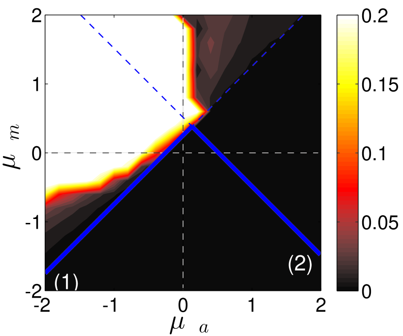
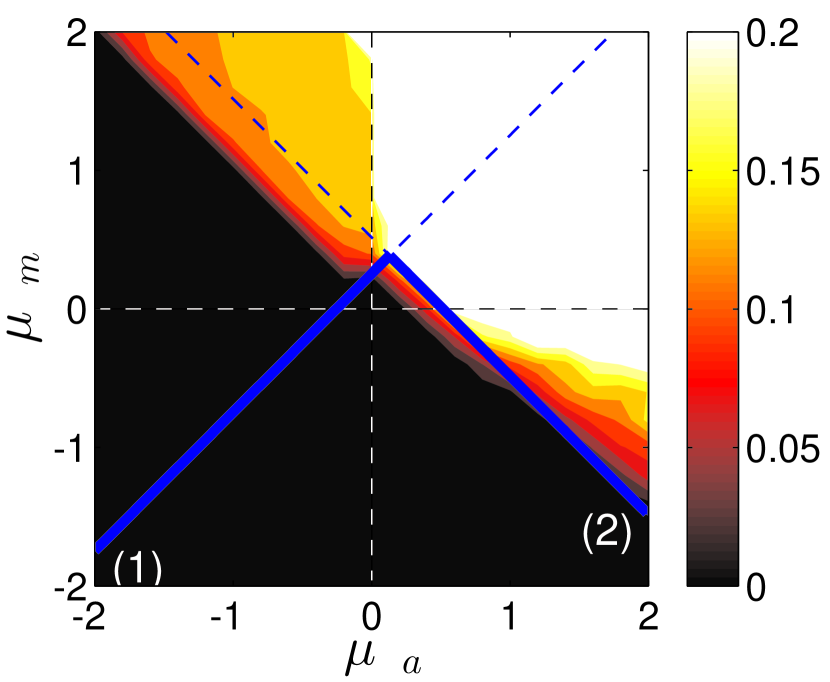
ρ0=10.0subscript𝜌010.0\rho_{0}=10.0

Φtsubscriptdelimited-⟨⟩Φ𝑡\langle\Phi\rangle_{t}

Refer to caption

Ψtsubscriptdelimited-⟨⟩Ψ𝑡\langle\Psi\rangle_{t}

Refer to caption

ρ0=2.5subscript𝜌02.5\rho_{0}=2.5

Φtsubscriptdelimited-⟨⟩Φ𝑡\langle\Phi\rangle_{t}

Refer to caption

Ψtsubscriptdelimited-⟨⟩Ψ𝑡\langle\Psi\rangle_{t}

Refer to caption
Figure 7: Comparison of numerical simulations of the individual-based model with the predictions of the hydrodynamic theory on the stability of the disordered solution in the (μm,μa)subscript𝜇𝑚subscript𝜇𝑎(\mu_{m},\mu_{a})-plane for different densities: ρ0=10.0subscript𝜌010.0\rho_{0}=10.0 (L=20𝐿20L=20, top) and ρ0=2.5subscript𝜌02.5\rho_{0}=2.5 (L=40𝐿40L=40, bottom). Left: Average orientational order parameter Φtsubscriptdelimited-⟨⟩Φ𝑡\langle\Phi\rangle_{t}; Right: Average spatial inhomogeneity order parameter Ψtsubscriptdelimited-⟨⟩Ψ𝑡\langle\Psi\rangle_{t}. The solid blue (gray) lines show the critical lines for the instability of the disordered solution. Line (1) corresponding to the orientation instability (2.1dadfgijm), whereas line (2) corresponds to the clustering instability (2.1dadfgijpqrsv). Other parameters: Dφ=0.06subscript𝐷𝜑0.06D_{\varphi}=0.06, N=4000𝑁4000N=4000, μr=5subscript𝜇𝑟5\mu_{r}=5, lc=0.2subscript𝑙𝑐0.2l_{c}=0.2, ls=1subscript𝑙𝑠1l_{s}=1, s0=0.25subscript𝑠00.25s_{0}=0.25, dt=0.01𝑑𝑡0.01dt=0.01.

The emergence of collective motion as well as the destabilization of the homogeneous density distribution is mostly confirmed by the numerical individual-based simulations. In specific parameter regions, deviations from the hydrodynamic theory are observed.

In particular, we observe a high degree of collective motion in the effective-alignment region and strong deviations from the homogeneous spatial distribution of particles in the pure attraction regime as well as in the effective-alignment regime (in particular in the regime (μm,μa){(μm,μa):|μm|>|μa|,μm>0}subscript𝜇𝑚subscript𝜇𝑎conditional-setsubscript𝜇𝑚subscript𝜇𝑎formulae-sequencesubscript𝜇𝑚subscript𝜇𝑎subscript𝜇𝑚0\left(\mu_{m},\mu_{a}\right)\in\left\{\left(\mu_{m},\mu_{a}\right):|\mu_{m}|>|\mu_{a}|,\mu_{m}>0\right\}). This also confirms our previous results of comprehensive numerical investigations of related individual-based models [33, 28].

Disagreements between simulations and the theoretical prediction (non-vanishing orientational order and/or clustering in simulations below the two critical lines) appear predominantly close to the intersection of the two critical lines and are stronger at low densities. They might be associated with the mean-field assumptions used in order to derive the hydrodynamic theory. On the one hand, at low densities the assumption of a continuous density of neighbours is strongly violated. On the other hand, correlations between particles may play an important role in the respective parameter range (likewise for high densities). Thus, the factorization of the N-particle PDF into a product of one-particle PDFs (2.1de) leads to a questionable approximation in that case.

Another possible explanation for disagreement between theory and simulation is a breakdown of the homogeneous, disordered solution due to finite amplitude instabilities at parameters where this solution is still linearly stable.

For weak (or vanishing) short-ranged repulsion (lslcmuch-greater-thansubscript𝑙𝑠subscript𝑙𝑐l_{s}\gg l_{c} or μr|μm,a|much-less-thansubscript𝜇𝑟subscript𝜇𝑚𝑎\mu_{r}\ll|\mu_{m,a}|), we observe inhomogeneous states without polar order far in the effective anti-alignment regime (μm<0subscript𝜇𝑚0\mu_{m}<0, μa>0subscript𝜇𝑎0\mu_{a}>0), clearly below the critical line predicted by the hydrodynamic theory as shown in figure 8. This instability was missed in the previous study of the model [28]. We were able to confirm it, using our kinetic approach (see section 3) by positive eigenvalues of the matrix determining the stability of the disordered solution at the respective parameter values. A close inspection of the dynamics of the individual-based model in this parameter region reveals the emergence of dense nematic filaments with particles moving in an anti-parallel fashion within the filament, whereby approximately half of the particles moves in either direction along the filament (see figure 9).
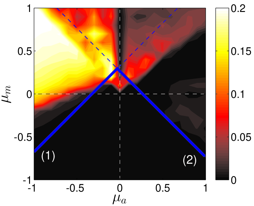
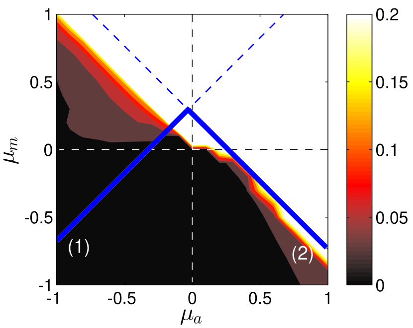
Φtsubscriptdelimited-⟨⟩Φ𝑡\langle\Phi\rangle_{t}

Refer to caption

Ψtsubscriptdelimited-⟨⟩Ψ𝑡\langle\Psi\rangle_{t}

Refer to caption
Figure 8: Results of numerical simulations on the stability of the disordered solution in the (μm,μa)subscript𝜇𝑚subscript𝜇𝑎(\mu_{m},\mu_{a})-plane for vanishing short-ranged repulsion (lc=0subscript𝑙𝑐0l_{c}=0). The spatial order parameter Ψtsubscriptdelimited-⟨⟩Ψ𝑡\left<\Psi\right>_{t} shows emergence of structures below the critical line (2). Other parameters: N=4000𝑁4000N=4000, ls=1subscript𝑙𝑠1l_{s}=1, s0=0.25subscript𝑠00.25s_{0}=0.25, Dφ=0.02subscript𝐷𝜑0.02D_{\varphi}=0.02, L=40𝐿40L=40.
Refer to caption
Figure 9: A sequence of snapshots of one simulation for different times visualizing the formation of nematic filaments for μa=0.6subscript𝜇𝑎0.6\mu_{a}=0.6, μm=0.4subscript𝜇𝑚0.4\mu_{m}=-0.4. The inset in (D) shows a close up of the spatial region indicated by the square in the upper left corner. Other parameters: N=4000𝑁4000N=4000, ls=1subscript𝑙𝑠1l_{s}=1, lc=0subscript𝑙𝑐0l_{c}=0, s0=0.25subscript𝑠00.25s_{0}=0.25, Dφ=0.02subscript𝐷𝜑0.02D_{\varphi}=0.02, L=36𝐿36L=36.

The hydrodynamic theory derived in section 4 is not able to account for this kind of structures as it considers only the (polar) momentum field and not the nematic director field as a coarse-grained variable. An extension of the hydrodynamic theory by including an equation for the nematic director field may allow for identifying instabilities due to the onset of nematic order, however it goes beyond the scope of this work. We refer the reader to some recent theoretical works on active nematics [34, 35, 39, 40, 21].

6 Discussion

The self-propelled particle model with selective attraction-repulsion interaction shows a rich dynamical behavior. In the “effective alignment” regime, characterized by repulsion from approaching agents and attraction to moving away agents, the model behavior is closely related to the well-known Vicsek model: For repulsion from approaching particles equal to, or stronger than, the attraction to particles moving away, we typically observe the homogeneous flocking phase with giant number fluctuations predicted by Toner and Tu. However, in the opposite case, if the attraction to particles moving away starts to dominate, we observe strong clustering and effective phase separation, which is not observed in minimal models with constant speed and velocity alignment. Furthermore, by continuously varying model parameters, we can observe other phases such as unpolarized clusters for pure attraction or dense filamentous nematic structures in the effective anti-alignment regime.

In order to obtain a fundamental understanding of the phase diagram of the model, we derived first a kinetic description of the system based on the Fourier transform of the probability density function. The corresponding system of equations for the successive Fourier modes can be used for efficient numerical analysis of the linear stability of solutions of the nonlinear Fokker-Planck equation. We have analyzed the stability of the spatially homogeneous solutions. In addition, we have shown that the integration over the social forces yields Bessel functions of the first kind, which enter the matrix elements of the corresponding linearized system of differential equations in Fourier space. Due to the alternating Taylor coefficients of the corresponding Bessel functions, a closure approximation, corresponding to a finite order expansion, immediately leads to unphysical divergences at large wavenumbers k𝑘k.

Furthermore, we have derived a hydrodynamic theory by truncating the “small-wavenumber-expansion” at the second order. The resulting hydrodynamic equations are in agreement with the generic Toner and Tu theory of active matter. Our work establishes a direct link between the microscopic parameters of the individual-based model and the macroscopic parameters governing the behaviour of the coarse-grained hydrodynamic variables (density and momentum fields). Interestingly, the hydrodynamic parameters, as for example η3subscript𝜂3\eta_{3}, which relates to a splay elasticity in corresponding equilibrium systems, or λ4subscript𝜆4\lambda_{4} and λ5subscript𝜆5\lambda_{5} which govern the relaxation of splay and bend fluctuations [mishra_fluctuations_2010], may change their sign in dependence on microscopic model parameters. Using the hydrodynamic theory, we can track down such sign changes to corresponding microscopic dynamics. Considering a limit of large system sizes, we reveal the importance of the change of sign of σ1subscript𝜎1\sigma_{1}, which indicates the transition from an overall aligning effect of the social interaction to the opposite case where the interaction tend to anti-align interacting particles. Finally, a comparison between the eigenvalues obtained from hydrodynamic theory and the kinetic description, which takes higher orders into account, allows us to assess the validity of the hydrodynamic theory.

We performed extensive simulations of the microscopic model based on stochastic differential equations focusing on the (μm,μa)subscript𝜇𝑚subscript𝜇𝑎(\mu_{m},\mu_{a})-plane in the parameter space. The critical lines obtained from the hydrodynamic theory, where the disordered, spatially homogeneous solution becomes unstable, show good agreement with the numerical results at sufficiently high densities. However, at certain parameters clear deviations appear, as for example in the vicinity of the crossing of the two critical lines at low densities.

This leads us to the important question of the validity of the approximations made during the coarse-graining. One common assumption is that of molecular chaos, which allows to factorize the N-particle PDF into a product of N one-particle PDFs. In models with collision-like interactions, the approximation is supposed to work best at low densities, where the mean-free path of particles between interactions is large[17, 19]. However, in our case, we observe large deviations at low densities. This contradicting effect may be due to an approximation required to evaluate the integrals over the social forces. It relies on a Taylor expansion of the one-particle density function around the position of a focal individual. However at low densities, the interaction range lssubscript𝑙𝑠l_{s} is not the suitable coarse-graining scale as assumed implicitly in the formulation of the one-particle Fokker-Planck equation. Similar arguments have been put forward also in [22]. The impact of individual (angular) noise on the mean-field assumption may also be not straight forward. Intuitively, one would argue that uncorrelated individual noise terms always decrease correlations between interacting particles. However, for self-propelled particles, angular noise leads to a stronger localization of particles [41, 42], thus in principle also to a prolonged interaction between neighbours, which may in principle enhance multi-particle correlations.

Furthermore, the systematic comparison of the prediction of the kinetic theory with the predictions of the hydrodynamic theory and numerical simulations revealed an unexpected additional instability. It corresponds to the emergence of dense filamentous structures with nematic order. Onset of nematic order is linked to the dynamics of the second Fourier amplitude, which was adiabatically eliminated in order to derive the hydrodynamic theory. Thus, the presented hydrodynamic theory cannot account for this instability, but it can be well traced by numerical evaluation of the linearized kinetic equations derived in section 3.

So far, hydrodynamic equations of active matter were derived directly from minimal microscopic models of self-propelled particles with velocity-alignment. Here, we show that it is also possible to derive such equations for a more complex model of self-propelled particles with selective attraction-repulsion interaction and establish a direct link between the microscopic and macroscopic level of description. The model exhibits a large variety of different phases and we believe, it might be not only of interest from the biological point of view, as an alternative to models including explicit alignment of individual agents, but that it offers also interesting playground for the study of self-organization, pattern formation and phase transitions at far-from-equilibrium conditions.

Appendix A Schematic Visualization of Social Interactions
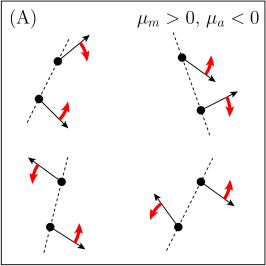
Refer to caption
Refer to caption
Refer to caption
Refer to caption
Figure 10: Turning of self-propelled particles due to the social interaction in the four regions of the (μm,μa)subscript𝜇𝑚subscript𝜇𝑎(\mu_{m},\mu_{a})-parameter space. In each panel, the left drawings corresponds to movement away v~ji>0subscript~𝑣𝑗𝑖0\tilde{v}_{ji}>0 and right drawings to approach v~ji<0subscript~𝑣𝑗𝑖0\tilde{v}_{ji}<0 of the agents. The red arrows indicate the torques acting on the agents, whereas the dashed line indicates the axis connecting the interaction partners, (anti-) parallel to the social forces; (A) effective alignment, (B) pure attraction, (C) pure repulsion and (D) effective anti-alignment.

Appendix B Calculation of K~p,nsubscript~𝐾𝑝𝑛\tilde{K}_{p,n} (2.1dt)

In this section, it is sketched, how the matrix elements K~p,n(k)subscript~𝐾𝑝𝑛k\tilde{K}_{p,n}(\bi{k}), defined by

K^p(k,t)subscript^𝐾𝑝kt\displaystyle{\hat{K}}_{p}(\bi{k},t) =2r02πφF(r,𝝋,t)eikr+ip𝝋,absentsuperscriptdifferential-d2𝑟superscriptsubscript02𝜋differential-d𝜑𝐹r𝝋tsuperscriptebold-⋅ikrip𝝋\displaystyle=\int\rmd^{2}r\int_{0}^{2\pi}\rmd\varphi\,F(\bi{r},\varphi,t)e^{i\bi{k}\cdot\bi{r}+ip\varphi}\,, (B.1a)
K^p(k,t)subscript^𝐾𝑝kt\displaystyle{\hat{K}}_{p}(\bi{k},t) =r=K~p,r(k)g^r(k,t)absentsuperscriptsubscript𝑟subscript~𝐾𝑝𝑟ksubscriptbold-^grkt\displaystyle=\sum_{r=-\infty}^{\infty}\tilde{K}_{p,r}(\bi{k}){\hat{g}}_{r}(\bi{k},t) (B.1b)

and used for the stability analysis of the spatial homogeneous solutions (2.1dk) of the Fokker-Planck equation (2.1dh) in section 3.2, are calculated. K~p,nsubscript~𝐾𝑝𝑛\tilde{K}_{p,n} is obtained by inserting the inverse Fourier transform of the one-particle PDF

p(r,𝝋,t)=1(2𝝅)3n=2kg^n(k,t)eikrin𝝋𝑝r𝝋t1superscript2𝝅3superscriptsubscriptnsuperscriptdifferential-d2ksubscriptbold-^gnktsuperscriptebold-⋅ikrin𝝋\displaystyle p(\bi{r},\varphi,t)=\frac{1}{(2\pi)^{3}}\sum_{n=-\infty}^{\infty}\int\rmd^{2}k\,{\hat{g}}_{n}(\bi{k},t)e^{-i\bi{k}\cdot\bi{r}-in\varphi} (B.2)

into (2.1dg) and solving the remaining integral:

Fφ(r,𝝋,t)=subscript𝐹𝜑r𝝋tabsent\displaystyle F_{\varphi}(\bi{r},\varphi,t)= 1(2π)3p=d2kg^p(k,t)eikr𝝋𝝋+2𝝅d𝝋jeip𝝋j{2s0𝐬𝐢𝐧(𝝋𝝋j2)\displaystyle\frac{1}{(2\pi)^{3}}\sum_{p=-\infty}^{\infty}\int\mbox{d}^{2}k\,{\hat{g}}_{p}(\bi{k},t)e^{-i\bi{k}\cdot\bi{r}}\int_{\varphi}^{\varphi+2\pi}\mbox{d}\varphi_{j}e^{-ip\varphi_{j}}\left\{2s_{0}\sin\left(\frac{\varphi-\varphi_{j}}{2}\right)\right.\, (B.3)
lclsdrjirji[μm(rji)φ+φj2φ+φj2+πdαeikrjisin(αφ)sin(φ+φj2α)\displaystyle\int_{l_{c}}^{l_{s}}\mbox{d}r_{ji}\,r_{ji}\left[\mu_{m}(r_{ji})\int_{\frac{\varphi+\varphi_{j}}{2}}^{\frac{\varphi+\varphi_{j}}{2}+\pi}\mbox{d}\alpha\,e^{-i\bi{k}\cdot\bi{r}_{ji}}\sin(\alpha-\varphi)\sin\left(\frac{\varphi+\varphi_{j}}{2}-\alpha\right)\right.
μa(rji)φ+φj2+πφ+φj2+2πdαeikrjisin(αφ)sin(φ+φj2α)]\displaystyle\left.-\mu_{a}(r_{ji})\int_{\frac{\varphi+\varphi_{j}}{2}+\pi}^{\frac{\varphi+\varphi_{j}}{2}+2\pi}\mbox{d}\alpha\,e^{-i\bi{k}\cdot\bi{r}_{ji}}\sin(\alpha-\varphi)\sin\left(\frac{\varphi+\varphi_{j}}{2}-\alpha\right)\right]
0lcrjirjiμr(rji)02παsin(αφ)eikrji}.\displaystyle\left.-\int_{0}^{l_{c}}\rmd r_{ji}\,r_{ji}\,\mu_{r}(r_{ji})\int_{0}^{2\pi}\rmd\alpha\,\sin(\alpha-\varphi)e^{-i\bi{k}\cdot\bi{r}_{ji}}\right\}\,.

In order to perform the integration over α𝛼\alpha and φjsubscript𝜑𝑗\varphi_{j}, the following identity is used to express the exponential function

eikrji=J0(krji)+2s=1(i)sJs(krji)cos(s(αχ)),superscript𝑒bold-⋅𝑖ksubscriptrjisubscript𝐽0𝑘subscript𝑟𝑗𝑖2superscriptsubscript𝑠1superscript𝑖𝑠subscript𝐽𝑠𝑘subscript𝑟𝑗𝑖𝑠𝛼𝜒\displaystyle e^{-i\bi{k}\cdot\bi{r}_{ji}}=J_{0}(k\,r_{ji})+2\sum_{s=1}^{\infty}(-i)^{s}J_{s}(k\,r_{ji})\cos\left(s\left(\alpha-\chi\right)\right)\,, (B.4)

where k=k(𝐜𝐨𝐬𝝌,𝐬𝐢𝐧𝝌)kk𝝌𝝌\bi{k}=k\left(\cos\chi,\sin\chi\right) and rji=rji(𝐜𝐨𝐬𝜶,𝐬𝐢𝐧𝜶)subscriptrjisubscriptrji𝜶𝜶\bi{r}_{ji}=r_{ji}\left(\cos\alpha,\sin\alpha\right). The Bessel functions of the first kind are denoted by Jν(x)subscript𝐽𝜈𝑥J_{\nu}(x).

Performing the integration yields the force expanded into a Fourier series and as a linear combination (B.1b) of the Fourier coefficients g^r(k,t)subscript^𝑔𝑟kt{\hat{g}}_{r}(\bi{k},t), where one can read off the elements of the infinite dimensional matrix K~p,n(k)subscript~𝐾𝑝𝑛k\tilde{K}_{p,n}(\bi{k}):

K~p,n(k)=subscript~𝐾𝑝𝑛kabsent\displaystyle\tilde{K}_{p,n}(\bi{k})= s0π22i{(μ~m,0(k)μ~a,0(k))(δp,1δn,1δp,1δn,1)+(μ~m,2(k)μ~a,2(k))\displaystyle\frac{s_{0}\pi^{2}}{2i}\left\{\left(\tilde{\mu}_{m,0}(k)-\tilde{\mu}_{a,0}(k)\right)\left(\delta_{p,1}\delta_{n,1}-\delta_{p,-1}\delta_{n,-1}\right)+\left(\tilde{\mu}_{m,2}(k)-\tilde{\mu}_{a,2}(k)\right)\right. (B.5)
[e2iχ(δp,1δn,1δp,2δn,0)e2iχ(δp,1δn,1δp,2δn,0)]}\displaystyle\left.\left[e^{-2i\chi}\left(\delta_{p,-1}\,\delta_{n,1}-\delta_{p,-2}\,\delta_{n,0}\right)-e^{2i\chi}\left(\delta_{p,1}\,\delta_{n,-1}-\delta_{p,2}\,\delta_{n,0}\right)...\right]\right\}
+2π2μ~r(k)δn,0(eiχδp,1eiχδp,1)+2s0s=0(1)s(μ~m,2s+1(k)+μ~a,2s+1(k))2superscript𝜋2subscript~𝜇𝑟𝑘subscript𝛿𝑛0superscript𝑒𝑖𝜒subscript𝛿𝑝1superscript𝑒𝑖𝜒subscript𝛿𝑝12subscript𝑠0superscriptsubscript𝑠0superscript1𝑠subscript~𝜇𝑚2𝑠1𝑘subscript~𝜇𝑎2𝑠1𝑘\displaystyle+2\pi^{2}\tilde{\mu}_{r}(k)\,\delta_{n,0}\left(e^{i\chi}\,\delta_{p,1}-e^{-i\chi}\,\delta_{p,-1}\right)+2s_{0}\sum_{s=0}^{\infty}(-1)^{s}\left(\tilde{\mu}_{m,2s+1}(k)+\tilde{\mu}_{a,2s+1}(k)\right)
[Λp,sei(2s+1)χδp+2s+1,nΓp,sei(2s+1)χδp(2s+1),n].delimited-[]subscriptΛ𝑝𝑠superscript𝑒𝑖2𝑠1𝜒subscript𝛿𝑝2𝑠1𝑛subscriptΓ𝑝𝑠superscript𝑒𝑖2𝑠1𝜒subscript𝛿𝑝2𝑠1𝑛\displaystyle\left[\Lambda_{p,s}\,e^{-i(2s+1)\chi}\,\delta_{p+2s+1,n}-\Gamma_{p,s}\,e^{i(2s+1)\chi}\,\delta_{p-(2s+1),n}\right]\,.

The following coefficients were introduced:

μ~m,ν(k)subscript~𝜇𝑚𝜈𝑘\displaystyle\tilde{\mu}_{m,\nu}(k) =lclsrjirjiμm(rji)Jν(krji),absentsuperscriptsubscriptsubscript𝑙𝑐subscript𝑙𝑠differential-dsubscript𝑟𝑗𝑖subscript𝑟𝑗𝑖subscript𝜇𝑚subscript𝑟𝑗𝑖subscript𝐽𝜈𝑘subscript𝑟𝑗𝑖\displaystyle=\int_{l_{c}}^{l_{s}}\rmd r_{ji}\,r_{ji}\,\mu_{m}(r_{ji})J_{\nu}(k\,r_{ji})\,, (B.6a)
μ~a,ν(k)subscript~𝜇𝑎𝜈𝑘\displaystyle\tilde{\mu}_{a,\nu}(k) =lclsrjirjiμa(rji)Jν(krji),absentsuperscriptsubscriptsubscript𝑙𝑐subscript𝑙𝑠differential-dsubscript𝑟𝑗𝑖subscript𝑟𝑗𝑖subscript𝜇𝑎subscript𝑟𝑗𝑖subscript𝐽𝜈𝑘subscript𝑟𝑗𝑖\displaystyle=\int_{l_{c}}^{l_{s}}\rmd r_{ji}\,r_{ji}\,\mu_{a}(r_{ji})J_{\nu}(k\,r_{ji})\,, (B.6b)
μ~r(k)subscript~𝜇𝑟𝑘\displaystyle\tilde{\mu}_{r}(k) =0lcrjirjiμr(rji)J1(krji),absentsuperscriptsubscript0subscript𝑙𝑐differential-dsubscript𝑟𝑗𝑖subscript𝑟𝑗𝑖subscript𝜇𝑟subscript𝑟𝑗𝑖subscript𝐽1𝑘subscript𝑟𝑗𝑖\displaystyle=\int_{0}^{l_{c}}\rmd r_{ji}\,r_{ji}\,\mu_{r}(r_{ji})J_{1}(k\,r_{ji})\,, (B.6c)
Λp,ssubscriptΛ𝑝𝑠\displaystyle\Lambda_{p,s} =32p(2s1)(1+2s)(3+2s)(1+2p+2s)(1+2p+2s)(3+2p+2s),absent32𝑝2𝑠112𝑠32𝑠12𝑝2𝑠12𝑝2𝑠32𝑝2𝑠\displaystyle=\frac{32p}{(2s-1)(1+2s)(3+2s)(-1+2p+2s)(1+2p+2s)(3+2p+2s)}\,, (B.6d)
Γp,ssubscriptΓ𝑝𝑠\displaystyle\Gamma_{p,s} =32p(2s1)(1+2s)(3+2s)(1+2p2s)(1+2p2s)(3+2p2s).absent32𝑝2𝑠112𝑠32𝑠12𝑝2𝑠12𝑝2𝑠32𝑝2𝑠\displaystyle=\frac{32p}{(2s-1)(1+2s)(3+2s)(-1+2p-2s)(1+2p-2s)(-3+2p-2s)}\,. (B.6e)

The Bessel functions Jν(x)subscript𝐽𝜈𝑥J_{\nu}(x) are oscillating functions with alternating Taylor coefficients. A truncation of the Taylor series (as done in section 4) at a finite order may therefore lead to unphysical behaviour for large wavenumbers k𝑘k.

Appendix C Algebraic Sign of the Transport Coefficients

Besides the coefficient η1subscript𝜂1\eta_{1}, which is always positive, all transport coefficients may be of either sign, positive or negative. In the following, the sign of every coefficient is discussed in the (μm,μa)subscript𝜇𝑚subscript𝜇𝑎(\mu_{m},\mu_{a})-parameter plane. For simplicity, it is assumed, that the interaction strengths μasubscript𝜇𝑎\mu_{a} and μmsubscript𝜇𝑚\mu_{m} do not depend on the distance between two particles.

λ1subscript𝜆1\lambda_{1} is positive above a critical line (positive slope and ordinate-intercept γ1subscript𝛾1\gamma_{1}) which is given by

μmμa=8Dφπρ0s02(ls2lc2)=:γ1>0,\displaystyle\mu_{m}-\mu_{a}=\frac{8D_{\varphi}}{\pi\rho_{0}s_{0}^{2}(l_{s}^{2}-l_{c}^{2})}\;{=:}\;\gamma_{1}>0\,, (C.1)

whereas λ2subscript𝜆2\lambda_{2} is positive above a critical line (negative slope and positive ordinate-intercept γ2subscript𝛾2\gamma_{2}), given by

μm+μa=27π16s0ρ0(ls3lc3)(s022+πρ0μrlc36)=:γ29π32s0lc3ls3lc3μr>0.\displaystyle\mu_{m}+\mu_{a}=\frac{27\pi}{16s_{0}\rho_{0}(l_{s}^{3}-l_{c}^{3})}\left(\frac{s_{0}^{2}}{2}+\frac{\pi\rho_{0}\mu_{r}l_{c}^{3}}{6}\right)\;{=:}\;\gamma_{2}\geq\frac{9\pi}{32s_{0}}\frac{l_{c}^{3}}{l_{s}^{3}-l_{c}^{3}}\,\mu_{r}>0\,. (C.2)

The analysis of the coefficient λ4subscript𝜆4\lambda_{4} is somewhat more involved. λ4subscript𝜆4\lambda_{4} is greater than zero inside a parabola, which is oriented along the line

μm+μa=405πs0256ρ0(ls3lc3)=:γ3>0.\displaystyle\mu_{m}+\mu_{a}=\frac{405\pi s_{0}}{256\rho_{0}\left(l_{s}^{3}-l_{c}^{3}\right)}\;{=:}\;\gamma_{3}>0\,. (C.3)

The width of the parabola is proportional to the noise strength Dφsubscript𝐷𝜑D_{\varphi} and inverse proportional to the density ρ0subscript𝜌0\rho_{0}. The vertex of the parabola has the coordinates

μa(v)=12(405πs0256ρ0(ls3lc3)+25s042πρ0(ls4lc4)Dφ),superscriptsubscript𝜇𝑎𝑣12405𝜋subscript𝑠0256subscript𝜌0superscriptsubscript𝑙𝑠3superscriptsubscript𝑙𝑐325superscriptsubscript𝑠042𝜋subscript𝜌0superscriptsubscript𝑙𝑠4superscriptsubscript𝑙𝑐4subscript𝐷𝜑\displaystyle\mu_{a}^{(v)}=\frac{1}{2}\left(\frac{405\pi s_{0}}{256\rho_{0}(l_{s}^{3}-l_{c}^{3})}+\frac{25s_{0}^{4}}{2\pi\rho_{0}(l_{s}^{4}-l_{c}^{4})D_{\varphi}}\right)\,, (C.4a)
μm(v)=12(405πs0256ρ0(ls3lc3)25s042πρ0(ls4lc4)Dφ).superscriptsubscript𝜇𝑚𝑣12405𝜋subscript𝑠0256subscript𝜌0superscriptsubscript𝑙𝑠3superscriptsubscript𝑙𝑐325superscriptsubscript𝑠042𝜋subscript𝜌0superscriptsubscript𝑙𝑠4superscriptsubscript𝑙𝑐4subscript𝐷𝜑\displaystyle\mu_{m}^{(v)}=\frac{1}{2}\left(\frac{405\pi s_{0}}{256\rho_{0}(l_{s}^{3}-l_{c}^{3})}-\frac{25s_{0}^{4}}{2\pi\rho_{0}(l_{s}^{4}-l_{c}^{4})D_{\varphi}}\right)\,. (C.4b)

The parabola itself is given by777Equations (C.5) and (C.6) are much easier to visualize in new coordinates β1=μm+μasubscript𝛽1subscript𝜇𝑚subscript𝜇𝑎\beta_{1}=\mu_{m}+\mu_{a} and β2=μmμasubscript𝛽2subscript𝜇𝑚subscript𝜇𝑎\beta_{2}=\mu_{m}-\mu_{a}. The transformation basically corresponds to a rotation in the (μm,μa)subscript𝜇𝑚subscript𝜇𝑎(\mu_{m},\mu_{a})-parameter plane.

μmμa=8s04πρ0(ls4lc4)Dφsubscript𝜇𝑚subscript𝜇𝑎8superscriptsubscript𝑠04𝜋subscript𝜌0superscriptsubscript𝑙𝑠4superscriptsubscript𝑙𝑐4subscript𝐷𝜑\displaystyle\mu_{m}-\mu_{a}=\frac{8s_{0}^{4}}{\pi\rho_{0}(l_{s}^{4}-l_{c}^{4})D_{\varphi}} [(64ρ0(ls3lc3)135πs0)2(μm+μa)2\displaystyle\left[\left(\frac{64\rho_{0}(l_{s}^{3}-l_{c}^{3})}{135\pi s_{0}}\right)^{2}(\mu_{m}+\mu_{a})^{2}\right. (C.5)
32ρ0(ls3lc3)45πs0(μm+μa)1].\displaystyle\left.\;-\frac{32\rho_{0}(l_{s}^{3}-l_{c}^{3})}{45\pi s_{0}}\,(\mu_{m}+\mu_{a})-1\right]\,.

The coefficient λ5subscript𝜆5\lambda_{5} is positive above the main diagonal, i.e. μm>μasubscript𝜇𝑚subscript𝜇𝑎\mu_{m}>\mu_{a}. Transport coefficient η2subscript𝜂2\eta_{2} is less than zero inbetween two hyperbolas, which are bounded by the asymptotes (C.1) and (C.3). The hyperbolas are determined by

μmμa=γ3(μm+μa)(μm+μa)γ1subscript𝜇𝑚subscript𝜇𝑎subscript𝛾3subscript𝜇𝑚subscript𝜇𝑎subscript𝜇𝑚subscript𝜇𝑎subscript𝛾1\displaystyle\mu_{m}-\mu_{a}=\gamma_{3}\,\frac{\left(\mu_{m}+\mu_{a}\right)}{\left(\mu_{m}+\mu_{a}\right)-\gamma_{1}} (C.6)

or rather

μm=12(γ1+γ3±4μa2+4μa(γ1γ3)+(γ1+γ3)2).subscript𝜇𝑚12plus-or-minussubscript𝛾1subscript𝛾34superscriptsubscript𝜇𝑎24subscript𝜇𝑎subscript𝛾1subscript𝛾3superscriptsubscript𝛾1subscript𝛾32\displaystyle\mu_{m}=\frac{1}{2}\left(\gamma_{1}+\gamma_{3}\pm\sqrt{4\mu_{a}^{2}+4\mu_{a}(\gamma_{1}-\gamma_{3})+(\gamma_{1}+\gamma_{3})^{2}}\right)\,. (C.7)

The extrema of the hyperbolas are located at

(μa(ext),μm(min))=(γ3γ12,(γ1γ3)22),superscriptsubscript𝜇𝑎𝑒𝑥𝑡superscriptsubscript𝜇𝑚𝑚𝑖𝑛subscript𝛾3subscript𝛾12superscriptsubscript𝛾1subscript𝛾322\displaystyle\left(\mu_{a}^{(ext)},\mu_{m}^{(min)}\right)=\left(\frac{\gamma_{3}-\gamma_{1}}{2},\frac{\left(\sqrt{\gamma_{1}}-\sqrt{\gamma_{3}}\right)^{2}}{2}\right)\,, (C.8a)
(μa(ext),μm(max))=(γ3γ12,(γ1+γ3)22).superscriptsubscript𝜇𝑎𝑒𝑥𝑡superscriptsubscript𝜇𝑚𝑚𝑎𝑥subscript𝛾3subscript𝛾12superscriptsubscript𝛾1subscript𝛾322\displaystyle\left(\mu_{a}^{(ext)},\mu_{m}^{(max)}\right)=\left(\frac{\gamma_{3}-\gamma_{1}}{2},\frac{\left(\sqrt{\gamma_{1}}+\sqrt{\gamma_{3}}\right)^{2}}{2}\right)\,. (C.8b)

The critical line for η3=0subscript𝜂30\eta_{3}=0 depends on the noise strength, whereby the critical noise strength reads

Dφ(c)=675π2s03(ls2lc2)2048(ls3lc3).superscriptsubscript𝐷𝜑𝑐675superscript𝜋2superscriptsubscript𝑠03superscriptsubscript𝑙𝑠2superscriptsubscript𝑙𝑐22048superscriptsubscript𝑙𝑠3superscriptsubscript𝑙𝑐3\displaystyle D_{\varphi}^{(c)}=\frac{675\pi^{2}s_{0}^{3}(l_{s}^{2}-l_{c}^{2})}{2048(l_{s}^{3}-l_{c}^{3})}\,. (C.9)

η3subscript𝜂3\eta_{3} is positive, if

μm{>μaDφ(c)+DφDφ(c)Dφ,Dφ<Dφ(c),<μaDφ(c)+DφDφ(c)Dφ,Dφ>Dφ(c).subscript𝜇𝑚casesformulae-sequenceabsentsubscript𝜇𝑎superscriptsubscript𝐷𝜑𝑐subscript𝐷𝜑superscriptsubscript𝐷𝜑𝑐subscript𝐷𝜑subscript𝐷𝜑superscriptsubscript𝐷𝜑𝑐otherwiseformulae-sequenceabsentsubscript𝜇𝑎superscriptsubscript𝐷𝜑𝑐subscript𝐷𝜑superscriptsubscript𝐷𝜑𝑐subscript𝐷𝜑subscript𝐷𝜑superscriptsubscript𝐷𝜑𝑐otherwise\displaystyle\mu_{m}\cases{>\mu_{a}\cdot\frac{D_{\varphi}^{(c)}+D_{\varphi}}{D_{\varphi}^{(c)}-D_{\varphi}}\,,\quad D_{\varphi}<D_{\varphi}^{(c)}\,,\\ <\mu_{a}\cdot\frac{D_{\varphi}^{(c)}+D_{\varphi}}{D_{\varphi}^{(c)}-D_{\varphi}}\,,\quad D_{\varphi}>D_{\varphi}^{(c)}\,.} (C.10)

Please note, that the slope of the lines is bounded by one (Dφ=0subscript𝐷𝜑0D_{\varphi}=0) and minus one (Dφsubscript𝐷𝜑D_{\varphi}\rightarrow\infty), respectively. Hence, η3subscript𝜂3\eta_{3} is always positive for {(μa,μm):μa<0,|μa|<μm<|μa|}conditional-setsubscript𝜇𝑎subscript𝜇𝑚formulae-sequencesubscript𝜇𝑎0subscript𝜇𝑎subscript𝜇𝑚subscript𝜇𝑎\left\{(\mu_{a},\mu_{m}):\mu_{a}<0\,,-\left|\mu_{a}\right|<\mu_{m}<\left|\mu_{a}\right|\right\} and η3subscript𝜂3\eta_{3} always negative for {(μa,μm):μa>0,μa<μm<μa}conditional-setsubscript𝜇𝑎subscript𝜇𝑚formulae-sequencesubscript𝜇𝑎0subscript𝜇𝑎subscript𝜇𝑚subscript𝜇𝑎\left\{(\mu_{a},\mu_{m}):\mu_{a}>0\,,-\mu_{a}<\mu_{m}<\mu_{a}\right\}. All criteria discussed above are summarized in figure 11.
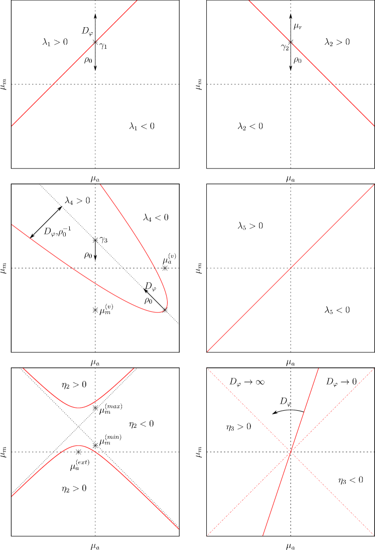
Refer to caption
Figure 11: The figure shows different regions in the (μm,μa)subscript𝜇𝑚subscript𝜇𝑎(\mu_{m},\mu_{a})-parameter space, where the transport coefficients have different algebraic signs. Critical lines, where the transport coefficients vanish, are drawn in red. Black arrows indicate the shift of characteristic points with increasing noise Dφsubscript𝐷𝜑D_{\varphi} and density ρ0subscript𝜌0\rho_{0}, respectively. See the main text for definitions.

The stability of the hydrodynamic equations (4.2) requires that both λ4subscript𝜆4\lambda_{4} and λ5subscript𝜆5\lambda_{5} are greater than zero. This is in principle true in the effective-alignment region (at least for sufficient high noise and low densities), as well as parts of the pure attraction and pure repulsion region. In this parameter region, the hydrodynamic equations describe collectively moving bands.

Appendix D Temperature Tensor

In [25, 23, 28], the symmetric temperature tensor

T^=(cosφ2cosφ2sinφcosφsinφcosφsinφcosφsinφcosφsinφ2sinφ2)^𝑇delimited-⟨⟩superscript𝜑2superscriptdelimited-⟨⟩𝜑2delimited-⟨⟩𝜑𝜑delimited-⟨⟩𝜑delimited-⟨⟩𝜑delimited-⟨⟩𝜑𝜑delimited-⟨⟩𝜑delimited-⟨⟩𝜑delimited-⟨⟩superscript𝜑2superscriptdelimited-⟨⟩𝜑2\hat{T}=\left(\begin{array}[]{cc}\left<\cos\varphi^{2}\right>-\left<\cos\varphi\right>^{2}&\left<\sin\varphi\cos\varphi\right>-\left<\sin\varphi\right>\left<\cos\varphi\right>\\ \left<\sin\varphi\cos\varphi\right>-\left<\sin\varphi\right>\left<\cos\varphi\right>&\left<\sin\varphi^{2}\right>-\left<\sin\varphi\right>^{2}\end{array}\right) (D.3)

is defined. It is a measure for the width of the velocity distribution (fluctuations around the mean velocity). The temperature is basically related to the second Fourier coefficients:

Txxsubscript𝑇𝑥𝑥\displaystyle T_{xx} =12(1+f^2(r,t)+f^2(r,t)2ρ(r,t))(f^1(r,t)+f^1(r,t)2ρ(r,t))2,absent121subscript^𝑓2rtsubscriptbold-^f2rt2𝜌rtsuperscriptsubscript^𝑓1rtsubscriptbold-^f1rt2𝜌rt2\displaystyle=\frac{1}{2}\left(1+\frac{{\hat{f}}_{2}(\bi{r},t)+{\hat{f}}_{-2}(\bi{r},t)}{2\rho(\bi{r},t)}\right)-\left(\frac{{\hat{f}}_{1}(\bi{r},t)+{\hat{f}}_{-1}(\bi{r},t)}{2\rho(\bi{r},t)}\right)^{2}\,, (D.4a)
Txysubscript𝑇𝑥𝑦\displaystyle T_{xy} =f^2(r,t)f^2(r,t)4iρ(r,t)(f^1(r,t))2(f^1(r,t))24i(ρ(r,t))2,absentsubscript^𝑓2rtsubscriptbold-^f2rt4𝑖𝜌rtsuperscriptsubscript^𝑓1rt2superscriptsubscript^𝑓1rt24𝑖superscript𝜌rt2\displaystyle=\frac{{\hat{f}}_{2}(\bi{r},t)-{\hat{f}}_{-2}(\bi{r},t)}{4i\rho(\bi{r},t)}-\frac{\left({\hat{f}}_{1}(\bi{r},t)\right)^{2}-\left({\hat{f}}_{-1}(\bi{r},t)\right)^{2}}{4i\left(\rho(\bi{r},t)\right)^{2}}\,, (D.4b)
Tyysubscript𝑇𝑦𝑦\displaystyle T_{yy} =12(1f^2(r,t)+f^2(r,t)2ρ(r,t))+(f^1(r,t)f^1(r,t)2ρ(r,t))2.absent121subscript^𝑓2rtsubscriptbold-^f2rt2𝜌rtsuperscriptsubscript^𝑓1rtsubscriptbold-^f1rt2𝜌rt2\displaystyle=\frac{1}{2}\left(1-\frac{{\hat{f}}_{2}(\bi{r},t)+{\hat{f}}_{-2}(\bi{r},t)}{2\rho(\bi{r},t)}\right)+\left(\frac{{\hat{f}}_{1}(\bi{r},t)-{\hat{f}}_{-1}(\bi{r},t)}{2\rho(\bi{r},t)}\right)^{2}\,. (D.4c)

The second Fourier coefficients are assumed to be fast variables in section 4.2, so that the temperature is implicitly contained in the hydrodynamic description of the system, even though the dynamics of the temperature tensor is not derived explicitly in this context.

References

References

  • [1] V. Schaller, C. Weber, C. Semmrich, E. Frey, and A. R. Bausch. Polar patterns of driven filaments. Nature, 467(7311):73–77, 2010.
  • [2] G. Salbreux, G. Charras, and E. Paluch. Actin cortex mechanics and cellular morphogenesis. Trends in Cell Biology, 22(10):536–545, October 2012.
  • [3] H. H. Wensink, J. Dunkel, S. Heidenreich, K. Drescher, R. E. Goldstein, H. Löwen, and J. M. Yeomans. Meso-scale turbulence in living fluids. Proceedings of the National Academy of Sciences, 109(36):14308–14313, September 2012.
  • [4] F. Peruani, J. Starruß, V. Jakovljevic, L. Søgaard-Andersen, A. Deutsch, and M. Bär. Collective motion and nonequilibrium cluster formation in colonies of gliding bacteria. Physical Review Letters, 108(9):098102, February 2012.
  • [5] I. Theurkauff, C. Cottin-Bizonne, J. Palacci, C. Ybert, and L. Bocquet. Dynamic clustering in active colloidal suspensions with chemical signaling. Physical Review Letters, 108(26):268303, June 2012.
  • [6] A. Kudrolli, G. Lumay, D. Volfson, and L. S. Tsimring. Swarming and swirling in self-propelled polar granular rods. Physical Review Letters, 100(5):058001, February 2008.
  • [7] J. Deseigne, O. Dauchot, and H. Chaté. Collective motion of vibrated polar disks. Physical Review Letters, 105(9):098001, 2010.
  • [8] M. Ballerini, N. Cabibbo, R. Candelier, A. Cavagna, E. Cisbani, I. Giardina, V. Lecomte, A. Orlandi, G. Parisi, A. Procaccini, M. Viale, and V. Zdravkovic. Interaction ruling animal collective behavior depends on topological rather than metric distance: Evidence from a field study. Proceedings of the National Academy of Sciences, 105(4):1232 –1237, January 2008.
  • [9] U. Lopez, J. Gautrais, I. D. Couzin, and G. Theraulaz. From behavioural analyses to models of collective motion in fish schools. Interface Focus, October 2012.
  • [10] J. Buhl, D. J. T. Sumpter, I. D. Couzin, J. J. Hale, E. Despland, E. R. Miller, and S. J. Simpson. From disorder to order in marching locusts. Science, 312(5778):1402–1406, June 2006.
  • [11] S. Bazazi, P. Romanczuk, S. Thomas, L. Schimansky-Geier, J. J. Hale, G. A. Miller, G. A. Sword, S. J. Simpson, and I. D. Couzin. Nutritional state and collective motion: from individuals to mass migration. Proceedings of the Royal Society B: Biological Sciences, 278(1704):356 –363, February 2011.
  • [12] T. Vicsek, A. Czirók, E. Ben-Jacob, I. Cohen, and O. Shochet. Novel type of phase transisition in a system of Self-Driven particles. Physical Review Letters, 75(6):1226–1229, 1995.
  • [13] J. Toner and Y. Tu. Long-Range order in a two-dimensional dynamical XY model: How birds fly together. Physical Review Letters, 75(23):4326, 1995.
  • [14] J. Toner and Y. Tu. Flocks, herds, and schools: A quantitative theory of flocking. Physical Review E, 58(4):4828–4858, 1998.
  • [15] J. Toner, Y. Tu, and S. Ramaswamy. Hydrodynamics and phases of flocks. Annals of Physics, 318(1):170–244, July 2005.
  • [16] S. Ramaswamy. The mechanics and statistics of active matter. Annual Review of Condensed Matter Physics, 1(1):323–345, August 2010.
  • [17] E. Bertin, M. Droz, and G. Grégoire. Boltzmann and hydrodynamic description for self-propelled particles. Physical Review E (Statistical, Nonlinear, and Soft Matter Physics), 74(2):022101–4, 2006.
  • [18] E. Bertin, M. Droz, and G. Grégoire. Microscopic derivation of hydrodynamic equations for self-propelled particles. Journal of Physics A: Mathematical and Theoretical, 42:445001, 2009.
  • [19] T. Ihle. Kinetic theory of flocking: Derivation of hydrodynamic equations. Physical Review E, 83(3):030901, March 2011.
  • [20] A. Peshkov, S. Ngo, E. Bertin, H. Chaté, and F. Ginelli. Continuous theory of active matter systems with metric-free interactions. Phys. Rev. Lett., 109:098101, August 2012.
  • [21] A. Peshkov, I. S. Aranson, E. Bertin, H. Chaté, and F. Ginelli. Nonlinear field equations for aligning self-propelled rods. Physical Review Letters, 109(26):268701, December 2012.
  • [22] F. D. C. Farrell, M. C. Marchetti, D. Marenduzzo, and J. Tailleur. Pattern formation in self-propelled particles with density-dependent motility. Phys. Rev. Lett., 108:248101, June 2012.
  • [23] R. Großmann, L. Schimansky-Geier, and P. Romanczuk. Active brownian particles with velocity-alignment and active fluctuations. New Journal of Physics, 14(7):073033, 2012.
  • [24] P. Romanczuk and U. Erdmann. Collective motion of active brownian particles in one dimension. The European Physical Journal Special Topics, 187(1):127–134, October 2010.
  • [25] P. Romanczuk and L. Schimansky-Geier. Mean-field theory of collective motion due to velocity alignment. Ecological Complexity, 10:83–92, June 2012.
  • [26] S. Mishra, K. Tunstrøm, I. D. Couzin, and C. Huepe. Collective dynamics of self-propelled particles with variable speed. Phys. Rev. E, 86:011901, July 2012.
  • [27] V. Guttal, P. Romanczuk, S. J. Simpson, G. A. Sword, and I. D. Couzin. Cannibalism can drive the evolution of behavioural phase polyphenism in locusts. Ecology Letters, 15(10):1158–1166, 2012.
  • [28] P. Romanczuk and L. Schimansky-Geier. Swarming and pattern formation due to selective attraction and repulsion. Interface Focus, 2(6):746–756, September 2012.
  • [29] Y.-L. Chou, R. Wolfe, and T. Ihle. Kinetic theory for systems of self-propelled particles with metric-free interactions. Phys. Rev. E, 86:021120, August 2012.
  • [30] I. N. Bronstein, K.A. Semendjajew, M. Gerhard, and H. Mühlig. Taschenbuch der Mathematik. Verlag Harri Deutsch, Frankfurt am Main, 7 edition, 2008.
  • [31] I. S. Aranson and L. S. Tsimring. Pattern formation of microtubules and motors: Inelastic interaction of polar rods. Phys. Rev. E, 71:050901, May 2005.
  • [32] S. Sankararaman, G. I. Menon, and P. B. Sunil Kumar. Self-organized pattern formation in motor-microtubule mixtures. Phys. Rev. E, 70:031905, September 2004.
  • [33] P. Romanczuk, I. D. Couzin, and L. Schimansky-Geier. Collective motion due to individual escape and pursuit response. Physical Review Letters, 102(1):010602–4, January 2009.
  • [34] S. Ramaswamy, R. A. Simha, and J. Toner. Active nematics on a substrate: Giant number fluctuations and long-time tails. Europhysics Letters (EPL), 62(2):196–202, April 2003.
  • [35] A. Baskaran and M. C. Marchetti. Hydrodynamics of self-propelled hard rods. Physical Review E, 77(1):011920, January 2008.
  • [36] S. Shinomoto and Y. Kuramoto. Phase transitions in active rotator systems. Prog. Theor. Phys., 75:1105-10,1986.
  • [37] H. Sakaguchi, S. Shinomoto, and Y. Kuramoto Phase transitions and their bifurcation analysis in a large population of active rotators with mean-field coupling. Prog. Theor. Phys., 79:600-7,1988.
  • [38] F.  Peruani, A. Deutsch, and M. Bär A mean-field theory for self-propelled particles interacting by velocity alignment mechanisms. The European Physical Journal Special Topics, 157:111-22,2008.
  • [39] F. Ginelli, F. Peruani, M. Bär, and H. Chaté. Large-scale collective properties of self-propelled rods. Physical Review Letters, 104(18):184502, 2010.
  • [40] S. Mishra, R. A. Simha, and S. Ramaswamy. A dynamic renormalization group study of active nematics. Journal of Statistical Mechanics: Theory and Experiment, 2010(02):P02003, February 2010.
  • [41] A. Mikhailov and D. Meinköhn. Self-motion in physico-chemical systems far from thermal equilibrium. In Lutz Schimansky-Geier and Thorsten Pöschel, editors, Stochastic Dynamics, volume 484 of Lecture Notes in Physics, pages 334–345. Springer Berlin Heidelberg, 1997.
  • [42] P. Romanczuk, M. Bär, W. Ebeling, B. Lindner, and L. Schimansky-Geier. Active Brownian particles. The European Physical Journal Special Topics, 202(1):1–162, March 2012.