Non-Markovian Equilibration Controlled by Symmetry Breaking

Abstract

We study the effects of symmetry breaking on non-Markovian dynamics in various system-bath arrangements. It is shown that by breaking certain symmetries features signaling non-Markovian time evolution disappear within a finite time $t_{g}$. We demonstrate numerically that the scaling of $t_{g}$ with the symmetry breaking strength is different for various types of symmetry. We provide a mathematical explanation for these differences related to the spectrum of the total system-bath Hamiltonian and provide arguments that the scaling properties of $t_{g}$ should be universal.

Introduction

Non-Markovian dynamics occurs in systems connected to a bath when information travels from the bath into the system. The name non-Markovian arises from the fact that these systems cannot be described by Markovian master equations Breuer(2002) ; Rivas(2012) ; Krovi(2007) . A system which is non-trivially joined to a finite bath will always be necessarily non-Markovian because any information which leaves the system must return Boccheri(1957) according to the Poincare recurrence theorum. In a generic finite system, the recurrence time is expected to scale exponentially with the size of the Hilbert spaceVenuti2010 . For many systems with a moderately sized finite bath, it may therefore be the case that significant non-Markovian events are only observable on timescales much longer than those of other relevant dynamics.

In order to define and quantify non-Markovianity in quantum systems different methods have been developed. For example, one can examine a distance measure between the actual evolution and the best Markovian model of a system bath arrangement. However, this approach is rarely used because of the difficulty of finding an optimum Markovian approximationWolf(2008) . There are other methods which involve examining the mathematical structure of the map defining the time evolution of the system Shabani(2009) ; Wilkie(2009) ; Budnini(2006) . Other techniques which have been proposed are based on determining the minimum amount of noise required to make the dynamics MarkovianWolf(2008) or studying the evolution of entanglement for a system prepared initially in a maximally entangled stateRivas(2010) .

Here we choose a method of studying the degree of non-Markovianity similar to the one proposed in Breuer2009 and further examined in Laine(2010) ; Breuer(2012) . Its central idea is to examine the trace distance between two different initial system states under time evolution (for examples of other methods and techniques, both analytic and numerical, see Krovi(2007) ; Wolf(2008) ; Breuer(2009-1) ; Breuer(2004) ; Churscinski(2010) ; vanWonderen(2006) ; Budnini(2006) ; Barnett(2001) ; Wilkie(2009) ; Daffler(2010) ; Kossakowski(2009) ; Shabani(2009) ; Rivas(2010) ; Breuer(2012) ; Wissmann2012 ; Piilo(2008) ). The trace distance is defined as

$$D_{\psi\psi^{\prime}}(t)=\mathrm{\frac{1}{2}Tr}(\sqrt{(\rho_{s}(t,|\psi_{0}\rangle)-\rho_{s}(t,|\psi^{\prime}_{0}\rangle))^{2}},$$ (1)

where $|\psi_{0}\rangle$ and $|\psi^{\prime}_{0}\rangle$ are two different initial states which are product states of the system and the bath with the same bath states but orthogonal system states. The system density matrix at a time $t$ is defined as

$$\rho_{s}(t,|\psi_{0}\rangle)=\mathrm{Tr}_{bath}(|\psi(t)\rangle\!\langle\psi(t)|),$$ (2)

$$|\psi(t)\rangle=\exp(-iH\>t)|\psi_{0}\rangle,$$

where $H$ is the overall system-bath Hamiltonian. A system is necessarily behaving in a non-Markovian fashion if the trace distance increases in time because of its interpretation as a measure of distinguishability. In general, the maximum of $D_{\psi\psi^{\prime}}(t)$ over all possible initial states has to be calculated (see Ref. Breuer2009 ). However, in the case where the system has only a few degrees of freedom, a single pair of orthogonal states can still provide valuable insights into the overall non-Markovian behavior of the system. Furthermore, examining non-Markovian behavior of a system by studying only two orthogonal initial states has the advantage that in numerical studies it is often impractical to maximize over all possible initial state pairs.

Non-Markovian systems have been studied intensively both theoretically and experimentally in recent years. On the experimental side the transition between Markovian and non-Markovian dynamics has been probed in optical setups Chiuri(2012) ; Liu(2011) . These experiments have been able to go from one regime to the other in a controllable way, thus allowing them to control the flow of information between system and bath. Non-Markovian effects have also been observed in solid state systems, for example with electron transport though a quantum dot Ubbelohde(2012) . Theoretically, recent research in the field of non-Markovian dynamics has been devoted to e.g. the study of memory effectsKrovi(2007) ; Churscinski(2010) ; Daffler(2010) , including examining the effect of bath memory on the equilibrium state of a system after evolving for a long timeChurscinski(2010) , the influence of a chaotic environment on non-Markovian dynamics Mata(2012) or the connection between non-Markovianty and entanglement Huelga(2012) . Interesting work has also been done in the study of multiple time correlation functions Alonso(2005) . We should also mention the vast theoretical effort to understand non-Markovianity in the framework of measurement theoryDiosi(2012) ; Gardiner(1985) ; Jack(1999) ; Jack(2000) ; Diosi(2008) ; Wiseman(2008) ; Diosi(2008)-1 ; Mazzola(2009) ; Gambetta(2003) . Still, our knowledge on the question how the internal structure of the bath influences the dynamics of the system is incomplete.

There have also been interesting studies on non-Markovian effects in a structured environment, using photonic crystals Florescu(2001) ; John(1995) as well as atoms on an optical lattice coupled to matter waves de Vega(2008) . The work in John(1995) is of particular relevance to this paper, because that work examined the effects of spontaneous symmetry breaking. This paper does not, however examine timescales of dynamical symmetry breaking as we do.

In this paper we demonstrate that non-Markovian dynamics can be controlled by breaking symmetries (e.g. parity) of the complete system-bath Hamiltonian. We show that non-Markovian events in the temporal evolution of the trace distance disappear on a certain time scale which depends on the strength of the symmetry breaking and give spectral arguments to show that the scaling behavior we observe is universal.

This paper is structured as follows. In Sec. I we explain the two system bath Hamiltonians studied in this paper, as well as the initial states and why they are chosen. In Sec. II we look at the dynamics of a tight binding torus, which has combined system-bath symmetry. In Sec. III we look at a 2 level qubit system coupled to a completely connected tight binding bath. In this case we break a symmetry which exists only in the bath. This is followed by a brief summary of conclusions. More detailed calculations are given in the supplemental material. Analysis of the bath correlations for the system bath arrangements considered in this paper is also provided in Sec. V.1 of the supplemental material.

I Setup

The first setup we study is a two-dimensional tight binding lattice whose dynamics is governed by the Hamiltonian

$$H_{2D}(g,N,r)=\sum_{<i,j>}^{N}c_{i}^{\dagger}c_{j}(1+g\>r_{ij}),$$ (3)

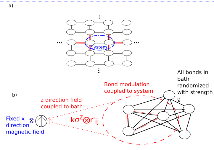
where $c_{i}$($c_{i}^{\dagger}$) is the annihilation (creation) operator on site i and $N$ is the number of sites in the lattice. The $<i,j>$ notation indicates that the sum is performed only over adjacent sites. $r_{ij}$ is a symmetric matrix, i.e. $r_{ij}=r_{ji}$ with the additional property $|r_{ij}|<1$, whose elements are chosen in a uniform random fashion. $g$ is a positive real number measuring the “strength” of the symmetry breaking. In the case of $g=0$ we recover the Hamiltonian of a particle which can move freely between the sites of the lattice. For finite values of $g$ the matrix elements of the Hamiltonian are altered randomly, which corresponds to altering the hopping rates between the sites. We initialize the system in the ground state of the Hamiltonian where 2 sites are disconnected. In the following these sites are referred to as the “system” and the remaining sites are referred to as the “bath”. At $t=0$ the system and the bath are joined in a “quench” process. Fig. 1a) shows the lattice and the quench. Evidently, the two eigenstates of the two site system Hamiltonian without any connection to the bath are a good choice of initial system states for the trace distance analysis.

The second setup we consider is a two-level (spin $\frac{1}{2}$) system coupled to a bath which is a fully connected graph. We have chosen a fully connected graph as the bath Hamiltonian because it has a very high degree of symmetry (symmetry under any permutation of sites) and therefore is a natural choice for examining the effects of symmetry breaking. The corresponding complete system-bath Hamiltonian is given by

$$H_{conn}(g,k,N,m,r,r^{\prime})=\sigma^{x}\otimes 1_{bath}+$$ (4)

$$1_{sys.}\otimes\sum_{i,j}^{N}c_{i}^{\dagger}c_{j}(1+g\>r_{ij})+k\>\sigma^{z}\otimes\sum_{p\neq q}^{m}c_{p}^{\dagger}c_{q}r^{\prime}_{pq},$$

which is of the canonical form $H=H_{sys.}\otimes 1_{bath}+1_{sys.}\otimes H_{bath}+k\>H_{sys.}^{coup}\otimes H_{bath}^{coup}$. As before, $r^{\prime}_{pq}$ and $r_{ij}$ are real symmetric matrices, ($r_{pq}^{\prime}=r_{qp}^{\prime}$, $r_{ij}=r_{ji}$) with the property $|r^{\prime}_{pq}|<1$ , $|r{}_{ij}|<1$. The elements of $r^{\prime}_{pq}$ and $r{}_{ij}$ are selected in a uniform random way. k measures the strength of the coupling between the system and the bath. For $k=0$ the system and the bath are completely decoupled. As k is increased a coupling is generated between the direction of the spin and the tunneling constants in the subset of sites 1 through m of the bath. We consider the case where $0<k\leq 1$. Depending on the sign of $r^{\prime}_{pq}$this coupling leads to either an increase or decrease in the hopping strength on each bond in the subset. If the direction of the system spin is switched, the hopping probabilities which were more favorable will become less favorable and vice versa. As in the first case g is a real number which measures the strength of the symmetry breaking. Fig. 1b) shows a sketch of this system-bath arrangement. For this Hamiltonian the spin is prepared in the +z (-z) direction and the bath is initiated with the lower energy quarter (25%) of its $k=0$ eigenstates filled with non-interacting particles. By means of this choice we can maximize the amount of information exchange between the system and the bath (for details see Sec. V.4). At $t=0$ a quench is performed when the spin-bath coupling $k$ is turned on.

Figure 1: Illustration of the two models studied in this paper a) system: 2 tight binding sites. bath: surrounding 2 dimensional tight-binding lattice b) system: single spin-$\frac{1}{2}$ in a magnetic field, bath: fully connected tight binding graph. Quench: system-bath coupling turned on at t=0.

We should also briefly discuss the definition of equilibration we use in this paper. We will consider a system to be equilibrated when remains near a stationary state which is relatively independent of the initial state for a long time. The trace distance measure we study serves as an indicator of equilibration, in the sense that it shows independence from the initial state. $D_{\psi\psi^{\prime}}(t)$ however cannot strictly be used as a measure of equilibration by itself because it does not provide information about weather or not the long time state of the system is a stationary state. The system is in fact equilibrating in both cases, as we demonstrate in section V.2 of the supplemental material.

II Two Dimensional Tight-binding Lattice with Combined System-Bath Symmetry

Figure 2: a) Trace distance versus time for two 10x10 lattices, (red) circles are for a torus and (cyan) diamonds are for a strip. b) Trace distance versus time for a 10x10 torus at half filling for various strengths of randomness g. g=0 (dotted blue line), g=0.02 (dashed red line), g=0.05 (solid green line), g=0.1 (dot dashed purple line). c) Timescale at which recurrences disappear, $t_{g}$ versus g for 10x10 torus at half filling, upper solid noisy (blue) line is the mean of $t_{g}$and the dashed (green) line is a linear fit. The lower solid (red) line is the median of $t_{g}$and the dot-dashed (black) line the corresponding linear fit. d) Non-Markovianity measure $\mathscr{N}(t,\Delta t;D)$ with $\Delta t=1000$ (blue) Xes are the mean of the measure for 400 realizations from $t=0$, (red) squares are the measure performed on the mean trace distance at times from $t=0$, (green) asterisks are the mean of the measure for times from $t=10^{8}$ and (black) diamonds are the measure of the mean at times from $t=10^{8}$ . All data in this plot are for small randomness, $g=10^{-6}$.

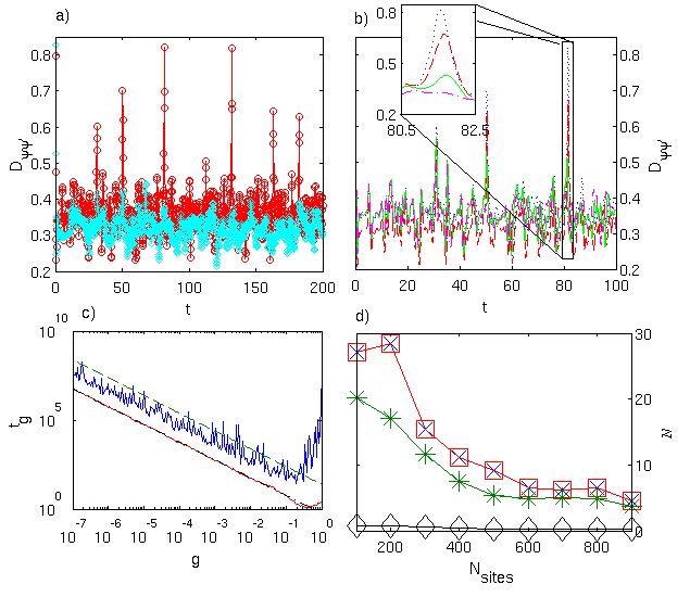
Let us now discuss how the trace distance $D_{\psi\psi^{\prime}}(t)$ evolves in time for the tight binding lattice. For a discussion concerning the numerical details, such as how we calculate the density matrix, we refer to the supplemental material (Sec. V.3). Fig. 2a) shows $D_{\psi\psi^{\prime}}(t)$ for two different boundary conditions applied to the Hamiltonian $H_{2D}$ given by Eq. 3. For periodic boundary conditions in x (x and y) we get a strip (torus). Since we monitor the temporal evolution of two orthogonal initial states the trace distance is one in the beginning of the dynamics when system and bath are joined together, that is $D_{\psi\psi^{\prime}}(t=0)=1$. Afterwards $D_{\psi\psi^{\prime}}(t)$ decreases rapidly in a short time, which is not visible in Fig. 2a) and then continues to fluctuate around a small value $D_{\psi\psi^{\prime}}(t=0)\approx 0.35$. In the case of the torus, which has the greater amount of symmetry of the two geometries, these fluctuations of the trace distance $D_{\psi\psi^{\prime}}(t)$ are interrupted by pronounced peaks. By performing a thorough analysis of the dynamics of the setup at these points in time we have found that these peaks can be explained by partial reconstructions of states which are similar to the initial states having a trace distance of one. In the following we elucidate this mechanism of state reconstruction.

For the torus the outgoing wavefunction from the initial state which is localized on the system sites propagates freely in both directions when the connections between the system and the bath are turned on. Eventually, it returns coherently to its initial position, reconstructing a wavefunction which is mostly isolated within the system. Similarly, the wavefunctions of the other states which initially have zero amplitude in the system reconstruct states with an approximately similar shape. On the contrary, for the strip geometry the wavefunctions are scattered off the open boundary such that they do not reconstruct coherently when they return. Formally, the torus has a $\mathbb{Z}_{N}\otimes\mathbb{Z}_{N}$ symmetry group whereas the strip only has the cyclic symmetry group $\mathbb{Z}_{N}$Kosmann-Schwarzbach (2010 . The larger symmetry group of the torus allows the wavefunction to preserve more of its shape while propagating. Therefore the torus allows for reconstructions which do not occur for the strip. Note that these reconstructions occur at a much shorter timescale than the recurrences which must occur because any finite closed quantum system must eventually return to a state arbitrarily close to its initial stateBoccheri(1957) . To avoid confusion we will refer to the features seen in Fig.2 a) as reconstructions and the features which must necessarily appear at long times as recurrences. Recurrences occur in the strip as well as any other geometry we could consider, but they occur at a much longer timescale than the partial reconstructions.

The coherence of the returning waves which partially reconstruct the initial state can be destroyed over time if randomness is introduced to the Hamiltonian. Fig. 2b) shows the temporal evolution of the trace distance $D_{\psi\psi^{\prime}}(t)$ in the case of the torus-geometry for different values of g, the strength of the random term. As the magnification in Fig. 2b) reveals the height of reconstruction peaks decreases with increasing $g$. In order to analyze this behavior we have studied how the time it takes for these peaks to disappear $t_{g}$ depends on the strength of the randomness $g$. Fig. 2c) shows $t_{g}$ as a function of $g$ in a double-logarithmic plot. As we can see from Fig. 2c) $t_{g}$ depends on $g$ in an inverse linear fashion, i.e.

$$t_{g}\propto\frac{1}{g}.$$ (5)

In the following we derive an intuitive understanding for this behavior. Evidently, the Hamiltonian of the complete system-bath arrangement has a discrete translational symmetry which leads to level-degeneracy in the energy spectrum. The addition of randomness breaks this symmetry and therefore leads to level splitting. For small randomness the gaps, which are created by the level splitting, are linearly proportional to $g$. The timescale associated with these gaps is simply their inverse which yields the dependency of $t_{g}$ on $g$ given by Eq. (5). The disappearance of the reconstruction by introducing randomness to the system-bath Hamiltonian peaks can be thought of as an equilibration process. We find that away from the reconstruction peaks the system density matrix is close to the fully equilibrated state for both initial conditions. The reconstructions drive the system away from this state, and therefore the system becomes more equilibrated as they are destroyed by symmetry breaking. The timescale $t_{g}$ with which these peaks disappear can therefore be thought of as a timescale for the equilibration of the system. (We also note that in Fig. 2c) the mean of $t_{g}$ is quite noisy and is much greater than the median. This indicates the presence of rare events where $t_{g}$ is very large.) In this case $t_{g}$ is defined as the timescale on which the reconstruction peaks no longer occur. Different $t_{g}$ can be observed for different choices of $r_{ij}$ from Eq.3. If we call $t_{g}$ for the kth random choice of $r_{ij}$ $t_{g}^{(k)}$, than the mean will be $t_{g}^{mean}=\sum_{k=1}^{m}\frac{t_{g}^{(k)}}{m}$. If the times are ordered such that $t_{g}^{(k)}\leq t_{g}^{(k+1)}$ than for m total samples, the median is $t_{g}^{median}=t_{g}^{(\frac{m}{2})}$.

Finally, we examine the effect of the reconstructions on the non-Markovianity of the system. To this end we calculate the total increase in trace distance over a given time period defined as

$$\mathscr{N}(t,\Delta t,D)=\intop_{t}^{t+\Delta t}d\tau[\frac{\partial D_{\psi\psi^{\prime}}(\tau)}{\partial\tau}\Theta(\frac{\partial D_{\psi\psi^{\prime}}(\tau)}{\partial\tau})],$$ (6)

where $\Theta$ is the Heavyside function and $D_{\psi\psi^{\prime}}(\tau)$ is defined in Eq. 1. $\mathscr{N}(t,\Delta t,D)$ is a measure of the information flowing from the bath into the system which allows us to distinguish between $\psi$ and $\psi^{\prime}$. It can therefore be thought of as the information allowing us to distinguish between $\psi$ and $\psi^{\prime}$ which would necessarily be lost by a Markovian approximation of the bath. Any time distinguishably between two arbitrary states is increasing the behavior of the system can be said to be non-MarkovianBreuer2009 . Fig. 2d) shows $\mathscr{N}(t,\Delta t,D)$ as a function of the number of system sites $N_{sites}$ at different points in time t with a fixed $\Delta t$. At early times the measure is the same for all realizations because the symmetry is not broken yet so the mean of the measure is the same as the measure of the mean. We see that with increasing time $\mathscr{N}(t,\Delta t,D)$ decreases systematically for all system sizes. Consequently, the evolution is less non-Markovian after the reconstruction peaks have disappeared. Furthermore, at times after the symmetry breaking has occurred, the average over different realizations of the system and bath does not show any increase. This indicates that any remaining non-Markovian features at these late times depend strongly on the details of the random symmetry breaking term. The fluctuations observed at these times are therefore not intrinsic dynamical fluctuations of the system, but a result of finite size and the presence of random symmetry breaking terms. Since the coupling between the system and bath is quite strong, there is no reason to expect Markovianity even asymptotically and in the large bath limit.

Moreover, Fig. 2d) reveals that as the system size $N_{sites}$ becomes larger the early and late non-Markovianity measures approach each other. An explanation for this is that as the system is made larger there is more time between the reconstructions. Thus the effect of the reconstructions is hidden by small fluctuations which transport information in and out of the system at all times.

III Fully Connected Graph Coupled to 2 Level System

Figure 3: a) Trace distance between two initially orthogonal states versus time for a bath consisting of 25 particles on 100 sites (N=100) with k=1 and m=20. Pluses (green) correspond to $g=0$, circles (red) to $g=10^{-3}$, and diamonds (black) to $g=10^{-1}.$ b) $t_{g}$ versus the strength of the randomness $g$ respectively the coupling parameter between system and bath $k$. The solid (blue) line is $t_{g}$ versus g for the same parameters as (a), the dot-dashed (magenta) line is the same but with $k=10^{-3}$. The dashed (red) line is $t_{g}$ versus k for g=1 and all other parameters the same as (a), the dotted (green) line is the same but with $g=10^{-3}$. c) $D_{\psi\psi^{\prime}}(t)$ for various system sizes with $k=1$, $m=\frac{N}{5}$, and quarter filling. Solid (blue) line is for $N=100$, dashed (green) $N=200$, dot-dashed (red) $N=300$, dotted (cyan) $N=400$, dashed (purple) $N=500$ and solid (gold) $N=600$. All plots are averaged over 400 realizations of the system-bath arrangement. d) Standard deviation of mean trace distance averaged over 400 samples for $g=10^{-4}$. Standard deviation of mean (red asterisks) and mean of standard deviation (green Xes) for times from $t=10^{5}$ to $t=10^{7}$, standard deviation of mean (black circles) and mean of standard deviation (blue squares), for times from $t=10^{9}$ to $t=10^{11}$.

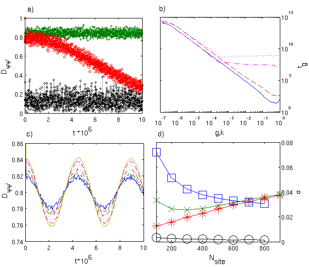
Let us now turn to the second setup which is a qubit coupled with a fully connected tight binding graph. Fig. 3a) shows the temporal evolution of the trace distance $D_{\psi\psi^{\prime}}(t)$ for different values of the randomness $g$. For $g=0$ we observe fluctuations of $D_{\psi\psi^{\prime}}(t)$ around $0.8$ after a rapid decrease from the initial value $D_{\psi\psi^{\prime}}(t=0)=1$. When the randomness is large, $g=10^{-1}$, the fluctuations occur at a much smaller value, that is $D_{\psi\psi^{\prime}}(t)\approx 0.2$. For moderate randomness, $g=10^{-3}$, the trace distance slowly decreases in time until it continues to fluctuate around an intermediate value between $0.2$ and $0.8$. Accordingly, it can be said that the system equilibrates to states with a much larger trace distance for $g=0$ compared to the case when $g$ is finite (see sec. V.2 of the supplementary materials for more information on why this can be considered equilibration) . In other words one can say that the unbroken permutation symmetry for $g=0$ prevents full equilibration for which we give a physical explanation in the next paragraph.

For $g=0$ the high degree of symmetry leads to many completely localized eigenstates in the part of the bath which is not connected to the system. Consequently, these parts of the wavefunction cannot contribute to the equilibration process. Hence for $g=0$ the system will never fully equilibrate. When a small randomness ($g\neq 0$) is added, these eigenstates acquire a finite amplitude to be in the part of the bath connected to the system and thus the system will eventually equilibrate. (see Sec. V.6)

Contrary to the first setup we observe in Fig. 3a) no peaks or systematic increases of the trace distance $D_{\psi\psi^{\prime}}(t)$ which would correspond to a flow of information from the bath into the system. Consequently, one could draw the conclusion that the second setup shows no systematic non-Markovian dynamics which do not depend on the details of $r^{\prime}_{pq}$ and $r_{ij}$. However, this is not true and we will return to this problem at a later point in the manuscript.

Let us now ask how the strength of the random term $g$ affects the equilibration time $t_{g}$ which we define as the time when the trace distance drops below $0.4$. In Fig. 3b) $t_{g}$ versus $g$ is shown in a double logarithmic plot. As we can see the equilibration time scales as

$$t_{g}\propto\frac{1}{g^{2}}.$$ (7)

as long as $g$ is sufficiently small compared to the coupling parameter $k$. Furthermore, we observe that if $g$ is large compared to $k$ the equilibration time $t_{g}$ does not depend on $g$.

The physical reason for the different dependencies of the equilibration time $t_{g}$ on the strength of the randomness $g$ for the two studied setups (compare Eqs. 5 and 7) can be traced back to the spectrum of the system bath Hamiltonian. Both Hamiltonians show a level splitting which is proportional to $g$. Nevertheless, this level splitting leaves a gap degeneracy in the case of the fully connected bath by gap degeneracy we mean that the gaps between certain energy eigenvalues of the overall Hamiltonian are the same, in this case the gap degeneracy is the result of pairs of energy levels having the same slope when the level degeneracy is split. We will later show that this gap degeneracy is effectively the same as a level degeneracy once we trace out the bath degrees of freedom. A demonstration that this happens whenever there is a symmetry in the bath which is not broken by coupling to the system can be found in Sec. IV.

As the next step we keep the randomness fixed and study how the equilibration time $t_{g}$ depends on the strength of the coupling between the system and the bath $k$. Fig. 3 b) shows that $t_{g}$ scales exactly as before in an inverse quadratic way, i.e.

$$t_{g}\propto\frac{1}{k^{2}},$$ (8)

which we are going to explain in the following. In this case the tensor product nature of the k=0 Hamiltonian produces a gap degeneracy. The tensor product structure of the coupling term in Eq. 4 means that this gap degeneracy cannot be broken by direct level splitting, but instead must be broken by level repulsion, for more details see Sec. V.5.

Now we return to question whether the dynamics of the second setup possesses hallmarks of systematic non-Markovianty or not. To do this we must compare the mean of the standard deviation of the trace distance, which shows all fluctuations, both intrinsic dynamical fluctuations and those related to the random symmetry breaking terms which is defined as

$$M_{\sigma}=\sum_{k=1}^{s}\frac{1}{s}\sqrt{\sum_{i=1}^{p}\frac{1}{p}(D_{\psi\psi^{\prime}}^{(k)}(t_{i})-\sum_{i=1}^{p}\frac{1}{p}D_{\psi\psi^{\prime}}^{(k)}(t_{i}))^{2}},$$ (9)

to the standard deviation of the mean

$$\sigma_{M}=\sqrt{\sum_{i=1}^{p}\frac{1}{p}(\sum_{k=1}^{s}\frac{1}{s}D_{\psi\psi^{\prime}}^{(k)}(t_{i})-\sum_{k=1}^{s}\frac{1}{s}\sum_{i=1}^{p}\frac{1}{p}D_{\psi\psi^{\prime}}^{(k)}(t_{i}))^{2}},$$ (10)

which only shows the intrinsic dynamical fluctuations.

We observe that Fig. 3a) shows no systematic increase of the trace distance $D_{\psi\psi^{\prime}}(t)$. Fig. 3c) shows an average of $D_{\psi\psi^{\prime}}(t)$ over 400 different realizations of $r^{\prime}_{pq}$ versus the bath size whereas the fraction $\frac{m}{N}$ is fixed and we choose $k=1$, $g=0$. Evidently, we observe systematic non-Markovian oscillations in Fig. 3c) which are masked by random fluctuations in Fig. 3a). Indeed these oscillations are systematic in the sense that they are not destroyed by averaging over different realizations. Increasing the bath size appears to actually increase the strength of the systematic oscillations. These oscillations are caused by internal bath dynamics where the bath sites which are not connected to the system effectively act as a single site, detailed calculations of how this happens can be found in Sec. V.6.

After the system has fully equilibrated the non-Markovian oscillations of the trace distance disappear as we can see from Fig. 3d) in which we examine the standard deviation of the trace distance at early (after the initial transient but before the symmetry is broken) and late (after the symmetry is broken) times. This can be seen because at late times the standard deviation of the mean over different choices of $r_{ij}$ and $r^{\prime}_{pq}$ drops to nearly zero. The drop to nearly zero means that the systematic oscillations have disappeared because the mean value over different realizations hardly fluctuates at all. At these late times we can see that there are fairly strong fluctuations in $D_{\psi\psi^{\prime}}(t)$, these fluctuations disappear however when we average over different realizations. The analogue of Fig. 3c) at late rather than early times would look like a flat line and not contain the sinusoidal oscillations we see at early times.

By examining the standard deviation of the mean trace distance compared to the mean of the standard deviation we can determine how sensitive the non-Markovian behavior is to the specific values of the randomly selected term $r^{\prime}_{pq}$ (and for late times also $r_{ij}$). As Fig. 3d) shows the standard deviation of the mean of trace distance at early times increases and is approached by the mean of the standard deviation for large system size. The closeness of these two numbers indicate that for large bath sizes the trace distance at early times is dominated by behaviors which are the same for most choices of $r^{\prime}_{pq}$ and do not depend much on the details of the random modulation of bond strengths. In contrast the standard deviation of the mean trace distance for late times is much less than the mean of the standard deviation for all system sizes, indicating that asymptotically the trace distance is dominated by random fluctuations strongly dependent on the details of $r_{ij}$ and $r^{\prime}_{pq}$.

In Fig. 3d) we examine the mean of the standard deviation of the trace distance over different random selections of $r_{ij}$ and $r^{\prime}_{pq}$, we also examine the standard deviation of the mean value of trace distance. The mean of the standard deviation tells us about the average variability of the trace distance before and after the symmetry is broken. This mean decreases with system size for late times and eventually becomes less than the value for early times for a bath with 800 total sites. This decrease with size is caused by a decrease in non-Markovian fluctuations associated with finite size effects as the bath is made bigger. In contrast the mean of the standard deviation for early times increases with system size as the trace distance oscillations shown in Fig. 3c) get stronger.

IV Spectral Arguments for the Universality of $t_{g}\propto\frac{1}{g^{2}}$ For bath symmetry breaking

Figure 4: (color online) a) Energy spectrum of the Hamiltonian for various strengths of g, dot-dashed (yellow) lines are eigenstates which are not initially part of a degenerate manifold of states for g=0, dotted (red) lines are states which are part of a degenerate manifold for g=0. A pair of eigenstates which are the same in the bath for g=0 are shown as sold (blue) lines. The slope of the energy of these two states is the same for small g but is changed by avoided crossings for larger g. b) Double logarithmic plot of the difference from the initial gap between pairs of states within the degenerate manifold which are the same in the bath for g=0 versus g.

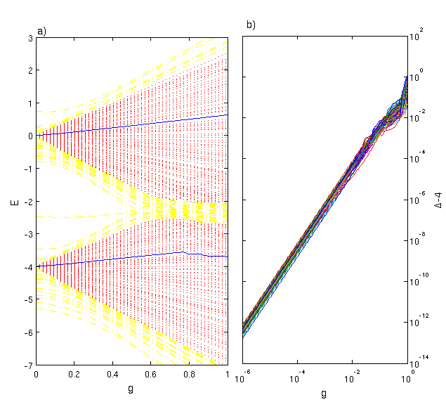
An explanation for why $t_{g}$ scales like $\frac{1}{g^{2}}$ rather than $\frac{1}{g}$ can be obtained by examining the energy spectrum of the Hamiltonian at different values of g. As we can see from Fig. 4a), the spectrum for g=0 is highly degenerate. As g is increased, the degeneracy is broken, however there will be pairs of states within the two manifolds which change energy with the same slope, as we can see from Fig. 4a). The gap between the energies of the states in these pairs will therefore remain the same until the slope of the energy is changed by an avoided crossing. The relevant process for equilibrating the system is not the splitting of the level degeneracy but rather the splitting of a gap degeneracy caused by avoided crossings. Because the slope is the same for each pair, the gap must change in a manner proportional to $g^{2}$ rather than g. We can verify that the gap increases proportionally to $g^{2}$ by looking at the double logarithmic plot of gap versus g shown in Fig. 4b).

The two degenerate manifolds in 4a) correspond to states where the particle in the bath is isolated in the sites which are not connected to the system. These two manifolds correspond to the two eigenstates of the system Hamiltonian. The total Hamiltonian can therefore be written in the form

$$H=(H^{\prime}{}_{sys}\otimes 1_{sym})\oplus H_{nosym}+g\>1_{sys}\otimes H_{break}.$$ (11)

This is the generic form of any system bath arrangement with a bath symmetry. In general we can always write $H_{break}=\lambda_{split}(H_{split}\oplus H_{2})+\lambda_{mix}H_{mix}$ where $H_{split}$ spans the same subspace as $1_{sym}$ in Eq.11. The Hamiltonian is now of the form

$$H = (H^{\prime}{}_{sys}\otimes 1_{sym}+g\>\lambda_{split}\>1_{sys}\otimes H_{split})$$

$$\oplus(H_{nosym}+g\>\lambda_{split}\>H_{2})+g\>\lambda_{mix}\>1_{sys}\otimes H_{mix}.$$

We can now construct a basis in the system such that $[|n\rangle\langle n|,H^{\prime}_{sys}]=0\;\forall|n\rangle$ and a basis in the bath such that $\langle i|1_{sym}|i\rangle=\begin{cases}1&|i\rangle\in deg.\\ 0&otherwise\end{cases}$ where deg. refers to the degenerate subspace created by the bath symmetry. For $\lambda_{mix}=0$ the density matrix of a system with an arbitrary initial state $|\psi_{0}\rangle$ can then be written as

$$\rho_{ijmn}(t) = \exp(-i\Delta_{mn}t)$$

$$\cdot (\sum_{l,k\in sym}A_{ijlkmn}\exp(-i\Delta_{ij}t))$$

$$+ \sum_{l\>or\>k\notin sym}A{}_{ijlkmn}\exp(-i\Delta{}_{lk}t),$$ (14)

$$A_{ijlkmn} = (\langle m|\otimes\langle i|)|l\rangle\left\langle l|\psi_{0}\right\rangle\left\langle\psi_{0}|k\right\rangle\langle k|(|j\rangle\otimes|n\rangle),$$

$$\Delta_{lk} = E_{l}-E_{k}$$

Where $|l\rangle$ and $|k\rangle$ are eigenstates of the overall Hamiltonian and $\Delta_{mn}=\left\langle m\mid H^{\prime}_{sys}\mid m\right\rangle-\left\langle n\mid H^{\prime}_{sys}\mid n\right\rangle$ is the gap between states within the different degenerate manifolds which is determined uniquely by n and m. We can now trace out the bath, yielding the system density matrix,

$$\rho_{nm}(t) = \sum_{q}(\exp(-i\Delta_{nm})(\sum_{l,k\in sym}A_{qqlkmn})$$

$$+ \sum_{l\>or\>k\notin sym}A{}_{qqlkmn}\exp(-\imath\Delta{}_{lk}t))$$

$$= \sum_{q}\left\langle q\mid\rho(t)\mid q\right\rangle.$$

Notice that all of the terms with $\Delta_{ij}\neq 0$ do not contribute to the final reduced density matrix, and therefore the sector of the bath containing $H_{split}$ cannot dephase the system. If $\lambda_{mix}\neq 0$ than level repulsion can occur with energy levels outside of the subspace as shown in Fig. 4, these level repulsions break the gap degeneracy and therefore destroy the tensor product structure in Eq. IV. As we can see from Fig. 4b) the gaps are widened proportionally to $g^{2}$ rather than g, therefore the timescale for the broken symmetry to equilibrate the system is proportional to $\frac{1}{g^{2}}$. The arguments given here will work for any case where a bath symmetry is broken, therefore for small g, $t_{g}\propto\frac{1}{g^{2}}$ for a generic bath symmetry being broken.

To make this argument more concrete, let us consider the case where we do not constrain the form of $H_{break}$, we can always write $H_{break}=(H_{spit}\oplus H_{2})+H_{mix}$, we note that only $H_{mix}$can break the gap degeneracy. We can further note that in this way of writing $H_{break}$ we can always choose $H_{mix}$ in such a way that it contains only off diagonal terms which mix between the sectors of the bath Hamiltonian with and without the degeneracy.

The only effect $H_{mix}$ can have on the energy levels within the degenerate subspace is though level repulsion with levels outside of this subspace (shown as dashed (yellow online) lines in Fig. 4 a). Let us consider the effect where 2 energy levels are initially separated by a gap $\Delta_{0}$ and an off diagonal term $g_{0}$ is added to split the degeneracy. For simplicity let us choose the zero of energy to lie half way between the 2 levels such that $E_{0}^{1}=\frac{\Delta_{0}}{2}=-E_{0}^{2}$. In this case we can easily find the energy as a function of $g_{0}$

$$E_{g}^{1}=\sqrt{\frac{\Delta_{0}^{2}}{4}+g_{0}^{2}}=\frac{\Delta_{0}}{2}+\frac{2g_{0}^{2}}{\Delta_{0}}+O(g_{0}^{4})$$ (16)

Because $g_{0}\propto g$ this implies that for small values of g the addition of a term $g\>H_{mix}$will cause the energies to deviate from their initial values in a manner proportional to $g^{2}$. The time scale associated with this modification of the spectrum will be inversely proportional to the splitting of the gap degeneracy, therefore $t_{g}\propto\frac{1}{g^{2}}$.

The case where more than 2 (but still finitely many) energy levels are simultaneously involved in level repulsion is slightly more complicated. In this case we can argue that because the energy is an analytic function of g for all finite (and zero) g, it can be represented as a perturbation series expanded around g=0,

$$E_{g}^{1}=a_{0}+a_{1}g+a_{2}g^{2}+\ldots+a_{\alpha}g^{\alpha}+\ldots.$$ (17)

The direct level splitting will always be the same for all sets of eigenvalues with the same bath state, and the energy levels will be initially degenerate. We have already show that $H_{split}$ cannot play a role in the equilibration. We can now further deduce that the first order contribution to the perturbation series from $H_{mix}$ vanishes because $\left\langle\phi_{split}\mid H_{mix}\mid\phi_{split}\right\rangle=0$ where $|\phi_{split}\rangle$ is an eigenvector of $H_{split}$. For this reason the constant and linear terms will not play a role in the equilibration. It is mathematically possible that the level repulsions are precisely balanced so that the term $a_{2}$ in Eq. 17 is equal to zero, in fact with enough energy levels it is mathematically possible to make all terms from $a_{2}$ up to $a_{\alpha-1}$, where $\alpha$ is a finite integer, be equal for all $E_{g}^{i}$ in the initially degenerate subspace. In this case we would have $t_{g}\propto\frac{1}{g^{\alpha}}$, such a case however is not typical in the sense that the repulsion strengths between levels would have to be precisely chosen for these terms in the perturbation series to be equal, and a small generic modification of the symmetry breaking term would restore the more universal behavior of $t_{g}\propto\frac{1}{g^{2}}$. Stated differently, for a given system bath arrangement, the set of symmetry breaking terms where $t_{g}$ does not scale like $\frac{1}{g^{2}}$ is a subset of measure zero of the set of all possible symmetry breaking terms which have the required bath symmetry.

Conclusions

In this work it has been shown that non-Markovian dynamics can be evoked by symmetry breaking. We have examined two examples of atypical equilibration which involve highly non-Markovian behavior for a period of time. In both of these examples, internal bath degrees of freedom play an important role. We have shown that these non-Markovian features are related to symmetries in the Hamiltonian, and that breaking these symmetries determines the timescales of their disappearance. Furthermore we have demonstrated that the effect of the symmetry breaking process is fundamentally different for symmetries of the overall system-bath Hamiltonian, compared to the breaking of symmetries which exist only in the bath, but are not broken by coupling to the system. There is a difference in the scaling of the equilibration timescale with the strength of the symmetry breaking. In the case of combined system-bath symmetry breaking this time scales inverse linearly with symmetry breaking strength, whereas when a symmetry only of the bath is broken, it scales inverse quadratically. This difference arises from the fact that for the breaking of a combined system-bath symmetry the relevant equilibration timescale is related to the breaking of level degeneracy, whereas in the case where a bath symmetry is broken the equilibration timescale relates to the breaking of gap degeneracies, in which the spacing between certain energy levels is the same. Because of the underlying spectral cause, these types of scaling are expected to be universal.

V Supplemental Material

V.1 Bath correlations for both systems

We can now examine the bath correlations, $|\left\langle B(0)\mid B(t)\right\rangle|$ for the two system bath arrangements considered in this paper. In the case of the torus, it is not immediately obvious how bath correlations should be defined, because there is not and underlying tensor product structure. In this case we will define B to be the part of the Hamiltonian which is turned on at t=0 and joins the system and bath.

Figure 5: (Color online) $|\left\langle B(0)\mid B(t)\right\rangle|$ versus time for 10x10 torus with the system initialized in a singlet state, and the bath initialized at half filling. Dotted (blue) line is for g=0, dashed (red) line is for g=0.01, solid (green) line is g=0.05 and dot-dashed (magenta) line is for g=0.1.

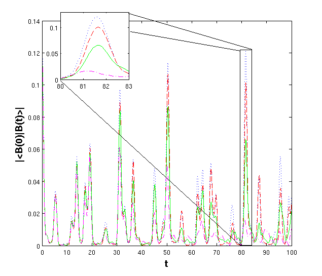
From Fig. 5 we can see that the bath correlations of the torus system bath arrangements show the same features that we observed in the trace distance. We notice peaks in this correlation which disappear on a timescale governed by g. We can also notice that the time for the bath correlations to initially decay is roughly 1 in units of coupling energy, and is independent of g.

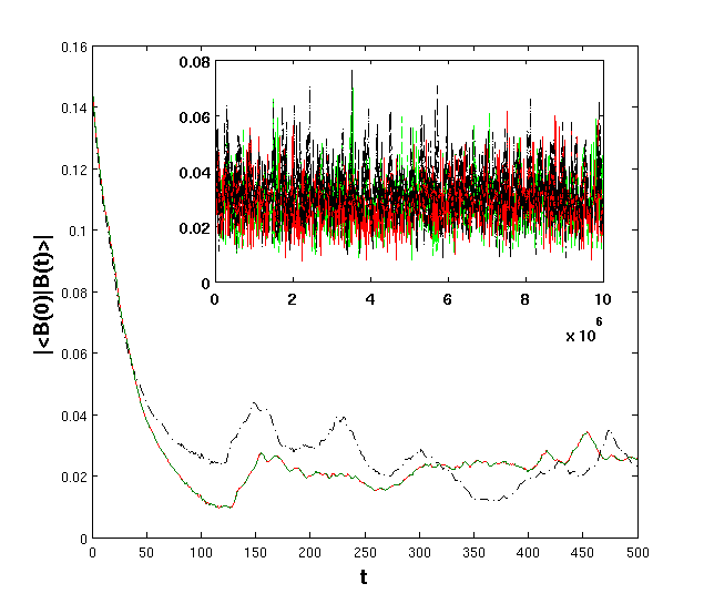
We can now also examine the bath correlations for the fully connected tight binding bath, in this case we define $B=\sum_{p\neq q}^{m}c_{p}^{\dagger}c_{q}r^{\prime}_{pq}$. From the inset of Fig. 6 we notice that the effect of the symmetry breaking is not visible from the bath correlations. We can also see from the main figure that the correlation decay time is roughly the same for all values of g and is on the order of $10^{2}$ in units of the coupling energy. The first revival of the bath correlations occurs on a similar timescale, and also appears not to depend on g. The relative independence of the details of the bath correlations on g indicates that the symmetry breaking effects observed in this system-bath arrangement are not well captured by the usual method of examining bath correlations.

Figure 6: (color online)$|\left\langle B(0)\mid B(t)\right\rangle|$ versus time for the fully connected arrangement for a bath consisting of 25 particles on 100 sites (N=100) with m=20. Dashed (green) lines correspond to $g=0$, solid (red) to $g=10^{-3}$, and dot-dashed (black) to $g=10^{-1}.$ Note that the lines for $g=0$ and $g=10^{-3}$ completely overlap throughout the main plot. Inset is the same quantities plotted over a longer timescale.

V.2 Von Neumann entropy of systems

As mentioned in the main text, showing that the trace distance becomes small does not rigorously demonstrate that the system is equilibrating. To show equilibration we need to demonstrate also that the system is near a stationary state. Trace distance does not allow us to access this information, but fortunately we can demonstrate this by examining the von Neumann entropy of one of the evolving states in each of the systems.

We choose to use base 2 von Neumann entropy, which has the formula

$$S_{VN}=\textrm{Tr}(\rho\log_{2}(\rho)).$$ (18)

The entropy in Eq. 18 is uniquely maximized by the totally dephased state $\rho_{dep}=\frac{1_{n}}{n}$ where n is the size of the system Hilbert space, in this case $S_{VN}^{max}=\log_{2}(n)$. We can clearly see that $\rho_{dep}$ will commute with any unitary time evolution operator and is therefore a stationary state. Therefore if $S_{VN}$ is close to $S_{VN}^{max}$than the system is close to a stationary state, thus fulfilling that criteria for equilibration. It is important to note that the converse is not true, stationary states do not necessarily have high $S_{VN}$, for example a pure density matrix made from an eigenstate of the Hamiltonian is stationary, but has $S_{VN}=0$.

Figure 7: (Color online) Von Neumann entropy versus time for 10x10 torus with the system initialized in a singlet state, and the bath initialized at half filling. Dotted (blue) line is for g=0, dashed (red) line is for g=0.01, solid (green) line is g=0.05 and dot-dashed (magenta) line is for g=0.1. The maximum possible entropy for this system is 2.

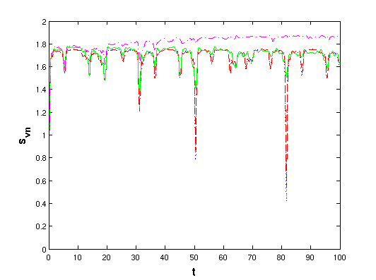
Allow us to first examine the von Neumann entropy for the torus arrangement, which can be seen in Fig. 7. We first note that because the system consists of 2 tight binding sites, the system density matrix is 4x4, meaning that the maximum $S_{VN}$ is 2. We see that except for during a reconstruction, this quantity is close to its maximum, indicating that the system is in fact near a stationary state. We can further notice from the plot for g=0.1 that the von Neumann entropy will increase slightly after the reconstructions have disappeared, this provided further evidence of an equilibration timescale related to the symmetry breaking.

Figure 8: Von Neumann entropy for the fully connected arrangement for a bath consisting of 25 particles on 100 sites (N=100) with k=1 and m=20. Dashed (green) lines correspond to $g=0$, solid (red) to $g=10^{-3}$, and dot-dashed (black) to $g=10^{-1}.$ The maximum possible entropy for this system is 1.

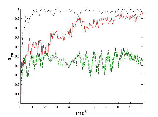
We now wish to perform the same analysis in the fully connected case. By examining Fig. 8 we can clearly see that at times greater than $t_{g}$ the von Neumann entropy approaches the maximum possible value of 1 for a single spin-$\frac{1}{2}$. We therefore can also conclude that the second system approaches a stationary state, and therefore equilibrates.

V.3 Details of density matrix construction for 2 dimensional graph

In this case we are considering a bosonic system and producing a reduced density matrix which combines the matrix elements for measuring a single particle on a site with those of measuring any finite (non-zero) number of particles on that site. For a two site system the density matrix for an individual wavefunction can be written as

$$\langle\psi|M|\psi\rangle$$ (19)

where

$$M_{i,j}=\begin{cases}0&\textrm{i or j =1}\\ {\displaystyle\sum_{i^{\prime}}^{<\delta_{i,2},\delta_{i,3}>}}|\phi_{i^{\prime}}\rangle\!\langle\phi_{i^{\prime}}|&i=j\neq 1\\ {\displaystyle\sum_{i^{\prime}}^{<\delta_{i,2},\delta_{i,3}>}\sum_{j^{\prime}}^{<\delta_{j,2},\delta_{j,3}>}}|\phi_{i^{\prime}}\rangle\!\langle\phi_{j^{\prime}}|&i\neq j\end{cases},$$

where $\delta_{i,j}$ is a Kronecker delta and <0,0> denotes the set of states where neither site is occupied, <1,0> denotes the state where site 1 is occupied and <0,1> denotes the state where site 2 is occupied. These single particle density matrices can then be combined into a 4x4 total density matrix by taking the product of density matrix elements to produce a combined density matrix using the following rule

$$\rho_{i,j}^{comb.}={\displaystyle\sum_{p,q,r,s}}B_{i}^{pq}B_{j}^{rs}\rho_{pr}^{1}\rho_{qs}^{2}$$ (20)

where B is a 4x4x4 tensor defined as

$$B_{1}^{pq} = \delta_{p=2q=3}+\delta_{p=3q=2}+\sum_{k=1}^{4}\delta_{p=1q=k}+\delta_{p=kq=1,}$$

$$B_{2}^{pq} = \delta_{p=2q=2}+\delta_{p=2q=4}+\delta_{p=4q=2,}$$

$$B_{3}^{pq} = \delta_{p=3q=3}+\delta_{p=3q=4}+\delta_{p=4q=3},$$

$$B_{4}^{pq} = \delta_{p=4q=4}.$$

These rules can be applied repeatedly to build up a full multi-particle density matrix. In this density matrix the fourth diagonal element corresponds to no particles on either site, the third diagonal element corresponds to a non-zero number of particles on site 2, but zero particles on site 1, the second corresponds to none on site 2 but a non-zero number on site 1, and the first corresponds to a non-zero number on both sites.

V.4 Estimate for long time mean of trace distance

Figure 9: Estimate of the long time mean of trace distance versus $\theta$, the angle between $\psi_{0}$ and the x-axis with $\psi^{\prime}_{0}$ chosen as the orthogonal state to $\psi_{0}$.

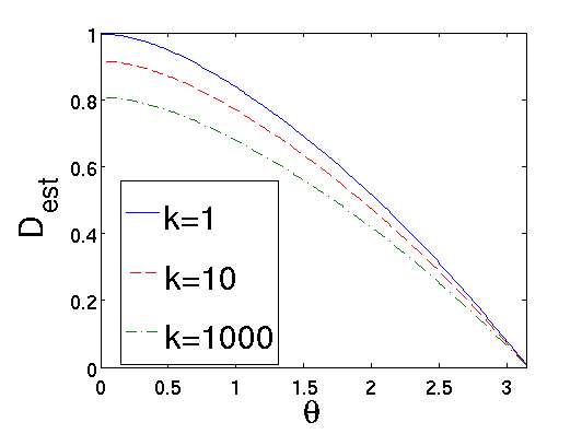
We now argue how the relevant non-Markovian dynamics of this system can be illuminated by observing only a single pair of orthogonal states. For the case of the spin system the choice of the two orthogonal initial states is not as obvious as it was for the torus. As in the case of 2d geometries, every possible choice of initial state in of the system has a single unique orthogonal partner. However, the best choice of initial state is not clear a priori. In the following we explain the choice of initial states for this setup. $H_{sys.}$ rotates spin vectors around the x-axis. Therefore, a rotation of the initial pair of states about this axis amounts to connecting the system to the bath at a different time. Fig. 9 demonstrates that the average trace distance should be smallest when $\psi_{0}$ is in the y-z plane. We can understand this intuitively because initial states pointing in the $\pm x$ direction are eigenstates of $H_{sys.}\otimes 1_{bath}+1_{sys.}\otimes H_{bath}$, whereas states in the y-z plane are only eigenstates of $1_{sys.}\otimes H_{bath}$. We want to examine states in which the maximum information travels into and out of the system, so we choose states in the y-z plane.

The estimate of the long time mean is calculated by totally dephasing (i.e. setting all off diagonal elements in the energy basis to zero) the total system-bath density matrix for the states $\psi_{0}$ and $\psi^{\prime}_{0}$ and calculating the trace distance between the resulting system density matrices. Let us call the totally dephased matrix $\rho_{\infty}$, for any operator A, $\textrm{Tr}[A\rho_{\infty}(|\psi_{0}\rangle)]=\int_{\tau=0}^{\infty}d\tau\textrm{Tr}[A\exp(-iH\>\tau)|\psi_{0}\rangle\!\langle\psi_{0}|\{\exp(iH\>\tau))]$, the long time mean of A. The trace distance can be though of as the maximum possible distinguishibility between systems with the two initial states using only measurements in the system, i.e. $D_{\psi\psi^{\prime}}(t)=\max_{A}(\textrm{Tr}[A\textrm{Tr}_{bath}[\rho(t,|\psi_{0}\rangle)]])-\textrm{Tr}[A\textrm{Tr}_{bath}[\rho(t,|\psi^{\prime}_{0}\rangle)]])$ where the eigenvalues of A are constrained to lie between 1 and 0. We therefore have for the trace distance between $\textrm{Tr}_{bath}[\rho_{\infty}(|\psi_{0}\rangle)]$ and $\textrm{Tr}_{bath}[\rho_{\infty}(|\psi^{\prime}_{0}\rangle)]$,

$$\max_{A}(\textrm{Tr}[A\textrm{Tr}_{bath}[\rho_{\infty}(|\psi_{0}\rangle)]])-\textrm{Tr}[A\textrm{Tr}_{bath}[\rho_{\infty}(|\psi^{\prime}_{0}\rangle)]])$$

$$= \max_{A}(\textrm{Tr}[A(\textrm{Tr}_{bath}[\rho_{\infty}(|\psi_{0}\rangle)]-\textrm{Tr}_{bath}[\rho_{\infty}(|\psi^{\prime}_{0}\rangle)])]$$

$$= \max_{A}(\textrm{Tr}[A(\textrm{Tr}_{bath}[\rho_{\infty}(|\psi_{0}\rangle)-\rho_{\infty}(|\psi^{\prime}_{0}\rangle)]]$$

$$= \max_{A}(\lim_{t\rightarrow\infty}\frac{1}{t}\int_{\tau=0}^{t}d\tau(\textrm{Tr}[A(\exp(-iH\>\tau)|\psi_{0}\rangle\!\langle\psi_{0}|\exp(iH\>\tau))$$

$$- \exp(-iH\>\tau)|\psi^{\prime}_{0}\rangle\!\langle\psi^{\prime}_{0}|\exp(\imath H\>\tau))]))$$

$$\lessapprox \lim_{t\rightarrow\infty}\frac{1}{t}\int_{\tau=0}^{t}d\tau(\max_{A}(\textrm{Tr}[A(\exp(-iH\>\tau)|\psi_{0}\rangle\!\langle\psi_{0}|\exp(iH\>\tau))$$

$$- \exp(-iH\>\tau)|\psi^{\prime}_{0}\rangle\!\langle\psi^{\prime}_{0}|\exp(iH\>\tau))]))$$

$$= \lim_{t\rightarrow\infty}\frac{1}{t}\int_{\tau=0}^{t}d\tau D_{\psi\psi^{\prime}}(\tau).$$

The trace distance between $\textrm{Tr}_{bath}[\rho_{\infty}(|\psi_{0}\rangle)]$ and $\textrm{Tr}_{bath}[\rho_{\infty}(|\psi_{0}^{\prime}\rangle)]$ gives the maximum average distinguishability between $\rho_{s}(t,|\psi_{0}\rangle)$ and $\rho_{s}(t,|\psi_{0}^{\prime}\rangle)$ assuming measurements are performed in the same basis at all times. The trace distance between the totally dephased states provides a lower bound for, and estimate of the average trace distance between $\rho_{s}(t,|\psi_{0}\rangle)$ and $\rho_{s}(t,|\psi_{0}^{\prime}\rangle)$ which is the maximum average distinguishability if measurements can be made in a different basis at every time.

V.5 Scaling arguments for $t_{g}$versus k

We can make very similar arguments to those given in Sec. IV of the main paper for why $t_{g}\propto\frac{1}{k^{2}}$. First let us consider the Hamiltonian of a system coupled to a bath in the canonical form

$$H=H_{sys.}\otimes 1_{bath}+1_{sys.}\otimes H_{bath}+k\>H_{sys.}^{coup}\otimes H_{bath}^{coup}.$$ (21)

Note that Hamiltonian given in Eq. 4 is of this form. We now note that we can decompose $H_{sys.}^{coup}\otimes H_{bath}^{coup}=D_{sys.}^{coup}\otimes D_{bath}^{coup}+R_{sys.}^{coup}\otimes R_{bath}^{coup}$ where $[D_{sys.}^{coup},H_{sys.}]=0$ and $[D_{bath}^{coup},H_{bath}]=0$. We now note that we can write $H_{sys.}\otimes 1_{bath}+1_{sys.}\otimes H_{bath}+k\>(D_{sys.}^{coup}\otimes D_{bath}^{coup}+R_{sys.}^{coup}\otimes R_{bath}^{coup})=H_{1}(k)+k\>R_{sys.}^{coup}\otimes R_{bath}^{coup}$ where $H_{1}(k)$ cannot equilibrate the bath by itself because $[D_{sys.}^{coup}\otimes D_{bath}^{coup},H_{sys.}\otimes 1_{bath}]=0$ and $[D_{sys.}^{coup}\otimes D_{bath}^{coup},1_{sys.}\otimes H_{bath}]=0$. In other words, a gap degeneracy will persist in $H_{1}(k)$ for any value of k. The gap degeneracy is broken by the term $k\>R_{sys.}^{coup}\otimes R_{bath}^{coup}$, however $R_{sys.}^{coup}\otimes R_{bath}^{coup}$ can always be chosen such that it contains only off diagonal elements in the energy basis of $H_{1}(k=0)$. The off diagonal elements can only change the spectrum though level repulsion rather than direct level splitting. The deviation from gap degeneracy will therefore scale like $k^{2}$rather than k, and as a result we observe $t_{g}\propto\frac{1}{k^{2}}$.

V.6 Eigenstates and eigenvalues of fully connected graph

Consider the Hamiltonian of a fully connected tight binding graph with equal coupling between all sites and zero on-site potential, $H_{c}=\sum_{i,j}^{N}c_{i}^{\dagger}c_{j}$. This Hamiltonian has a N-1 fold degenerate ground state manifold that spans all states for which the total amplitude sums to zero, i.e. $\sum_{i}\psi_{i}=0$. This can be shown in the case of zero on-site potential by observing that $(H_{c}\psi)_{i}=\sum_{j\neq i}\psi_{j}$. Therefore in the case where $\sum_{i}\psi_{i}=0$, we see that $(H_{c}\psi)_{i}=\sum_{j}\psi_{j}-\psi_{i}=-\psi_{i},$ these states therefore are eigenstates with eigenvalue -1. In the case where $\psi_{i}=\psi_{j}=\frac{\exp(\imath\phi)}{\sqrt{N}}$ we have $(H_{c}\psi)_{i}=\sum_{j\neq i}\psi_{j}=(N-1)\psi_{i}$, this state is therefore an eigenstate with an eigenvalue of N-1.

Now let us now consider a Hamiltonian of the form $H_{comb.}=H_{c}\oplus H_{a}+H_{join}$, where $H_{join}=\sum_{i=1}^{N}\sum_{j=N+1}^{N+M}c_{i}^{\dagger}c_{j}$ equally couples all N sites in $H_{c}$ to another group of sites, $H_{a}$ is an arbitrary Hamiltonian of size M. We now note that for an initial state $\psi$^trap such that $\sum_{i=1}^{N}\psi_{i}^{trap}=0$ and $\psi_{i}=0\;\forall\>i>N$. We can show that $\psi$^trap is an eigenstate of $H_{c}\oplus H_{a}$ because it has no support for $i>N$, and the part for $i\leq N$ is an eigenstate of $H_{c}$ with an eigenvalue of (N-1). We now also see that $(H_{join}\psi^{trap})_{i\leq N}=0$ and $(H_{join}\psi^{trap})_{i>N}=\sum_{i=1}^{N}\psi_{i}^{trap}=0$, therefore $H_{comb}$ will have an N-1 fold degenerate manifold of states which only have finite amplitudes in the first N sites and will have an energy of N-1. Wavefunctions in these states are effectively trapped in the first N sites.

We know by orthogonality of eigenstates, that all other eigenstates of $H_{comb}$ must have $\psi_{i}=\psi_{j}=\psi_{cc}$ for all i and j less then N+1. This constraint means that the internal degrees of freedom of the first N sites do not play a role in the eigenstates outside of the manifold mentioned in the previous paragraph. The first N sites can therefore be modeled as a single site.

References

- (1) H. P. Breuer and F. Petruccione, The Theory of Open Quantum Systems (Oxford University Press, 2002)
- (2) Á. Rivas and S. F. Huelga, Open Quantum Systems An Introduction (Springer, Berlin Heidelberg, 2012)
- (3) H.Krovi, O. Oreshkov, M. Ryazanov, and D.A. Lidar, Phys. Rev. A 76,052117 (2007).
- (4) P. Bocchieri and A. Loinger, Phys. Rev. 107, 337 (1957)
- (5) L.C. Venuti and P. Zanardi, Phys. Rev. A 81, 032113 (2010)
- (6) M. M. Wolf, J. Eisert, T. S. Cubitt and J. I. Cirac, Phys.Rev. Lett. 101, 150402 (2008).
- (7) A. Shabani and D. A. Lidar, Phys. Rev. Lett. 102, 100402 (2009).
- (8) J. Wilkie and Y. M. Wong, J. Phys. A 42, 015006 (2009).
- (9) A. A. Budini, Phys. Rev. A 74, 053815 (2006)
- (10) Á. Rivas, S. F. Huelga, and M. B. Plenio, Phys. Rev. Lett. 105, 050403 (2010)
- (11) H. P. Breuer, Phys. Rev. A 70, 012106 (2004).
- (12) H.P. Breuer, E.M. Laine, J Piilo PRL 103, 2104021 (2009)
- (13) E. M. Laine, J. Piilo and H. P. Breuer, Phys. Rev. A 81, p. 062115 (2010)
- (14) H. P. Breuer, J. Phys. B: At. Mol. Opt. Phys. 45 (2012)
- (15) S. Wissmann, A.Karlsson, E.M. Laine, J. Piilo, H.P. Breuer arXiv:1209.4989 (2012)
- (16) J. Piilo, S. Maniscalco, K. Härkö̈nen and K.-A. Suominen, Phys. Rev. Lett. 100, 180402 (2008); J. Piilo, K. Härkö̈nen, S. Maniscalco and K.-A. Suominen, Phys. Rev. A 79, 062112 (2009); H. P. Breuer and J. Piilo, Europhys. Lett. 85, 50004 (2009)
- (17) H. P. Breuer and B. Vacchini, Phys. Rev. Lett. 101, 140402 (2008); Phys. Rev. E 79, 041147 (2009).
- (18) A. J. van Wonderen and K. Lendi, Europhys. Lett. 71, 737 (2006).
- (19) S. M. Barnett and S. Stenholm, Phys. Rev. A 64,033808 (2001).
- (20) A. Kossakowski and R. Rebolledo, Open Syst. Inf. Dyn. 15, 135 (2008); Open Syst. Inf. Dyn. 16, 259 (2009).
- (21) D. Chruściński, A. Kossakowski and S. Pascazio, Phys. Rev. A 81, 032101 (2010).
- (22) S. Daffer, K. Wódkiewicz, J. D. Cresser and J. K. McIver, o Phys. Rev. A 70, 010304(R) (2004).
- (23) I. Garca-Mata, C. Pineda and D. Wisniacki, Phys. Rev. A 86, 022114 (2012).
- (24) A. Chiuri, C. Greganti, L. Mazzola, M. Paternostro and P. Mataloni, Scientific Reports 2, 968 (2012)
- (25) B.-H. Liu, L. Li, Y.-F. Huang, C.-F. Li, G.-C. Guo, E.-M. Laine, H.-P. Breuer and J. Piilo, Nature Physics 7, 931934 (2011).
- (26) N. Ubbelohde, K. Roszak, F. Hohls, N. Maire, R. J. Haug & T. Novotný, Scientific Reports 2, 374 (2012)
- (27) S. F. Huelga, A. Rivas and M. B. Plenio, Phys. Rev. Lett. 108, 160402 (2012).
- (28) D. Alonso and I. de Vega, Phys. Rev. Lett. 94, 200403 (2005).
- (29) L. Diósi, Phys. Rev. A, 85, 034101 (2012).
- (30) C. W. Gardiner and M. J. Collett, Phys. Rev. A 31, 3761–3774 (1985).
- (31) M. W. Jack, M. J. Collett, and D. F. Walls, J opt. B 1, 452 (1999).
- (32) M.W.Jack and M.J.Collett, Phys. Rev. A 61, 062106 (2000).
- (33) L. Diósi, Phys. Rev. Lett. 100, 080401 (2008).
- (34) H. M. Wiseman and J. M. Gambetta, Phys. Rev. Lett. 101, 140401 (2008).
- (35) L. Diósi, Phys. Rev. Lett. 101, 149902(E) (2008).
- (36) L. Mazzola, S. Maniscalco, J. Piilo, K.-A. Suominen, and B. M. Garraway, Phys. Rev. A 80, 012104 (2009).
- (37) J. Gambetta and H. M. Wiseman, Phys. Rev. A 68, 062104 (2003).
- (38) M. Florescu and S. John, Phys. Rev. A. 64, 33801 (2001).
- (39) S. John, T. Quang, Phys. Rev. Lett. 74, 3419 (1995).
- (40) I. de Vega et. al PRL 101, 260404 (2008).
- (41) M. Diez, N. Chancellor, S. Haas, L.C. Venuti, P. Zanardi, Phys. Rev. A 82, 032113 (2010)
- (42) J. von Neumann, Zeitschrift für Physik 57, 30 (1929), see also the english translation by R. Tumulka at arXiv:1003.2133.
- (43) H. Tasaki, Phys. Rev. Lett. 80, 1373 (1998).
- (44) S. Popescu, A. J. Short, and A. Winter, Nature Physics 2, 754 (2006).
- (45) N. Linden, S. Popescu, A. J. Short, and A. Winter, Phys. Rev. E 79, 061103 (2009).
- (46) P. Reimann, Phys. Rev. Lett. 101, 190403 (2008).
- (47) S. Goldstein, J. L. Lebowitz, R. Tumulka, , and N. Zanghí (2010), 1003.2129.
- (48) M. A. Nielsen and I. L. Chuang, Quantum Computation and Quantum Information (Cambridge University Press, Cambridge, 2000)
- (49) Kosmann-Schwarzbach, Yvette. From Finite Groups to Lie Groups (Springer, New York 2010)