Cash Flow Entropy

Ulrich Kirchner
PO Box 72277, Parkview, 2122, South Africa
ulrich.kirchner@gmail.com
Simon Moolman
Department of Physics
University of the Witwatersrand
Johannesburg
Abstract

In this paper we aim to find a measure for the diversity of cash flows between agents in an economy. We argue that cash flows can be linked to probabilities of finding a currency unit in a given cash flow. We then use the information entropy as a natural measure of diversity. This leads to a hirarchical inequality measure, which includes the well-known Theil index as a special case, and a constraint on agent entropy differentials, i.e., the difference between cash inflow and outflow entropies. The last result is particularly intriguing as it formalises the fact that an economy must contain both, cash flow aggregating and cash flow diversifying agents.

1 Introduction

Most people, when inspecting their bank account statement, could make the following observation: while inflows tend to come in a few large payments (salary etc), outflows are much more dispersed (daily groceries, rent, monthly bills, etc). By considering the sources, destinations and relative sizes of the payments, it is possible to write down the probability of where a dollar of an agent’s income came from and where it is going. With this we can describe the difference between the large inflows and dispersed outflows in terms of the entropy of these probabilities.

Let us assume an economy in which no money is created or destroyed and in which, over a period, cash flows only occur between a set of discrete agents. Such an economy can clearly not exist if every agent’s cash flow situation is as above — few large inflows and many small outflows. There must be agents who collect small cash flows and pay out large sums. Examples which come to mind are generally companies, for example selling a mass produced product (small cash flows) and buying supplies and services in bulk (large payments).

This hints at the idea that the entropies of the inflow and outflow probabilities of all the agents in the economy must be related in some way.

This paper will be structured as follows: In Section 2 we formalize the cash flow-probability relationship and introduce information entropy to measure diversity. In Section 3 we examine the results for the simpler case of a steady-state economy. Section 4 contains examples for the two and three agent cases. This is followed by the Conclusion in Section 5. In the appendix we derive the information entropy subdivision property for the case of 2/3 possible outcomes.

2 Cash flows and probabilities

Let us assume that in an economy cash flows occur over a period of time between N𝑁N agents. Let ckjsubscriptsuperscript𝑐𝑗𝑘c^{j}_{k} represent the cash flow from agent j𝑗j to agent k𝑘k. This can be conviniently represented in a cash flow matrix, where each row corresponds to a source agent (upper index) and each column to a destination agent (lower index)

[c11cN1c1NcNN]delimited-[]subscriptsuperscript𝑐11subscriptsuperscript𝑐1𝑁missing-subexpressionsubscriptsuperscript𝑐𝑁1subscriptsuperscript𝑐𝑁𝑁\left[{\begin{array}[]{ccc}c^{1}_{1}&\cdots&c^{1}_{N}\\ \vdots&&\vdots\\ c^{N}_{1}&\cdots&c^{N}_{N}\end{array}}\right] (1)

With cash flow ckjsubscriptsuperscript𝑐𝑗𝑘c^{j}_{k} we can then associate a probability

pkj=defckjk,jckj.superscriptdefsubscriptsuperscript𝑝𝑗𝑘subscriptsuperscript𝑐𝑗𝑘subscript𝑘𝑗subscriptsuperscript𝑐𝑗𝑘p^{j}_{k}\stackrel{{\scriptstyle\mbox{\tiny def}}}{{=}}\frac{c^{j}_{k}}{\sum_{k,j}{c^{j}_{k}}}. (2)

which represents the likelihood that a random currency unit in the economy would have been part of cash flow ckjsubscriptsuperscript𝑐𝑗𝑘c^{j}_{k} (which assumes identifiable currency units). Note that “saving” would correspond to a cashflow cjjsubscriptsuperscript𝑐𝑗𝑗c^{j}_{j} from an agent j𝑗j to himself.

To measure the diversity of all cash flows in the economy we will use the information entropy

H=defj,kpkjlog2(pkj),superscriptdef𝐻subscript𝑗𝑘subscriptsuperscript𝑝𝑗𝑘subscript2subscriptsuperscript𝑝𝑗𝑘H\stackrel{{\scriptstyle\mbox{\tiny def}}}{{=}}-\sum_{j,k}p^{j}_{k}\log_{2}(p^{j}_{k}), (3)

which is measured in bits (due to the choice of 222 as the base of the logarithm). To simplify the notation let us extend this definition to “un-normalized” probabilities by defining a new function

K(x1,,xn)=defH(x1ixi,,xnixi).superscriptdef𝐾subscript𝑥1subscript𝑥𝑛𝐻subscript𝑥1subscript𝑖subscript𝑥𝑖subscript𝑥𝑛subscript𝑖subscript𝑥𝑖K(x_{1},\ldots,x_{n})\stackrel{{\scriptstyle\mbox{\tiny def}}}{{=}}H\left(\frac{x_{1}}{\sum_{i}x_{i}},\ldots,\frac{x_{n}}{\sum_{i}x_{i}}\right). (4)

An intriguing property of the information entropy is how it respects the grouping of possible outcomes. Lets say we group the N𝑁N possible outcomes into n<N𝑛𝑁n<N groups. The overall entropy can then be written as

H=Hg+jpjHj,𝐻subscript𝐻gsubscript𝑗subscript𝑝𝑗subscript𝐻𝑗H=H_{\mathrm{g}}+\sum_{j}p_{j}H_{j}, (5)

where pjsubscript𝑝𝑗p_{j} is the probability of the outcome being in group j𝑗j, Hjsubscript𝐻𝑗H_{j} is the “internal entropy” of group j𝑗j (entropy of the probabilities conditional on the fact that the outcome was in group j𝑗j), and

Hg=defjpjlog2pjsuperscriptdefsubscript𝐻gsubscript𝑗subscript𝑝𝑗subscript2subscript𝑝𝑗H_{\mathrm{g}}\stackrel{{\scriptstyle\mbox{\tiny def}}}{{=}}-\sum_{j}p_{j}\log_{2}p_{j} (6)

is the information entropy for the aggregate groups.

By applying above identity recursively to the probabilities corresponding to all possible cash flows one obtains a hirarchical set of inequality/diversity measures.

As a first step let us put all savings ciisubscriptsuperscript𝑐𝑖𝑖c^{i}_{i} in one group, and all remaining cash flows in another group. Using above identity we find

H=H{sc}+p{s}H{s}+p{c}H{c},𝐻subscript𝐻𝑠𝑐subscript𝑝𝑠subscript𝐻𝑠subscript𝑝𝑐subscript𝐻𝑐H=H_{\{sc\}}+p_{\{s\}}H_{\{s\}}+p_{\{c\}}H_{\{c\}}, (7)

where p{s}=defipiisuperscriptdefsubscript𝑝𝑠subscript𝑖subscriptsuperscript𝑝𝑖𝑖p_{\{s\}}\stackrel{{\scriptstyle\mbox{\tiny def}}}{{=}}\sum_{i}p^{i}_{i} and p{c}=1p{s}subscript𝑝𝑐1subscript𝑝𝑠p_{\{c\}}=1-p_{\{s\}} are the aggregate probability of a currency unit being in a “saving cash flow” and inter-agent cash flow respectively,

H{sc}=defp{s}log2(p{s})p{c}log2(p{s})superscriptdefsubscript𝐻𝑠𝑐subscript𝑝𝑠subscript2subscript𝑝𝑠subscript𝑝𝑐subscript2subscript𝑝𝑠H_{\{sc\}}\stackrel{{\scriptstyle\mbox{\tiny def}}}{{=}}-p_{\{s\}}\log_{2}(p_{\{s\}})-p_{\{c\}}\log_{2}(p_{\{s\}}) (8)

is a measure of diverisification between savings and spending,

H{s}=defK(c11,,cNN)superscriptdefsubscript𝐻𝑠𝐾subscriptsuperscript𝑐11subscriptsuperscript𝑐𝑁𝑁H_{\{s\}}\stackrel{{\scriptstyle\mbox{\tiny def}}}{{=}}K(c^{1}_{1},\ldots,c^{N}_{N}) (9)

is a measure of the saving diversity in the economy (it is highest when all agents have the same saving), and

H{c}=defK(c21,,cn1n)superscriptdefsubscript𝐻𝑐𝐾subscriptsuperscript𝑐12subscriptsuperscript𝑐𝑛𝑛1H_{\{c\}}\stackrel{{\scriptstyle\mbox{\tiny def}}}{{=}}K(c^{1}_{2},\ldots,c^{n}_{n-1}) (10)

is a measure of diversity for all inter-agent cash flows.

Cash flows can now be grouped by their origin or destination. We define the aggregated cash flows from agent j𝑗j and to agent k𝑘k excluding savings as

cj=defk,kjckjck=defj,jkckj.formulae-sequencesuperscriptdefsuperscript𝑐𝑗subscript𝑘𝑘𝑗subscriptsuperscript𝑐𝑗𝑘superscriptdefsubscript𝑐𝑘subscript𝑗𝑗𝑘subscriptsuperscript𝑐𝑗𝑘c^{j}\stackrel{{\scriptstyle\mbox{\tiny def}}}{{=}}\sum_{k,k\neq j}c^{j}_{k}\qquad c_{k}\stackrel{{\scriptstyle\mbox{\tiny def}}}{{=}}\sum_{j,j\neq k}c^{j}_{k}. (11)

The probabilities of finding a currency unit (which is not a saving) in the cash-out/in flows of an agent are

pj=cjicipk=cklclformulae-sequencesuperscript𝑝𝑗superscript𝑐𝑗subscript𝑖superscript𝑐𝑖subscript𝑝𝑘subscript𝑐𝑘subscript𝑙subscript𝑐𝑙p^{j}=\frac{c^{j}}{\sum_{i}c^{i}}\qquad p_{k}=\frac{c_{k}}{\sum_{l}c_{l}} (12)

We can now define probabilities similar to above, but within one of the cash flow groups to or from an agent for jk𝑗𝑘j\neq k

pk(j)=ckjcj(1δkj)p(k)j=ckjck(1δkj).formulae-sequencesubscriptsuperscript𝑝𝑗𝑘subscriptsuperscript𝑐𝑗𝑘superscript𝑐𝑗1subscriptsuperscript𝛿𝑗𝑘subscriptsuperscript𝑝𝑗𝑘subscriptsuperscript𝑐𝑗𝑘subscript𝑐𝑘1subscriptsuperscript𝛿𝑗𝑘p^{(j)}_{k}=\frac{c^{j}_{k}}{c^{j}}(1-\delta^{j}_{k})\quad p^{j}_{(k)}=\frac{c^{j}_{k}}{c_{k}}(1-\delta^{j}_{k}). (13)

This is the probability to find an arbitrary currency unit leaving/going to agent j𝑗j in a cash flow to/from agent k𝑘k. Evidently

kpk(j)=1jp(k)j=1formulae-sequencesubscript𝑘subscriptsuperscript𝑝𝑗𝑘1subscript𝑗subscriptsuperscript𝑝𝑗𝑘1\sum_{k}p^{(j)}_{k}=1\qquad\sum_{j}p^{j}_{(k)}=1 (14)

By grouping the cash flow by the originating agent (upper index) we find

H{c}=H+jpjHj,subscript𝐻𝑐superscript𝐻subscript𝑗superscript𝑝𝑗superscript𝐻𝑗H_{\{c\}}=H^{\prime}+\sum_{j}p^{j}H^{j}, (15)

where

H=defjpjlog2(pj)superscriptdefsuperscript𝐻subscript𝑗superscript𝑝𝑗subscript2superscript𝑝𝑗H^{\prime}\stackrel{{\scriptstyle\mbox{\tiny def}}}{{=}}-\sum_{j}p^{j}\log_{2}(p^{j}) (16)

is the entropy of the aggregate agent cash out-flow probabilities pjsuperscript𝑝𝑗p^{j} and

Hj=defkpk(j)log2(pk(j))superscriptdefsuperscript𝐻𝑗subscript𝑘subscriptsuperscript𝑝𝑗𝑘subscript2subscriptsuperscript𝑝𝑗𝑘H^{j}\stackrel{{\scriptstyle\mbox{\tiny def}}}{{=}}-\sum_{k}p^{(j)}_{k}\log_{2}(p^{(j)}_{k}) (17)

is the entropy of each agents cash outflows, i.e., the entropy of pk(j)subscriptsuperscript𝑝𝑗𝑘p^{(j)}_{k} for fixed j𝑗j. It is maximized if all cash flows from the agent are equal, and minimized (in which case it is zero) if there is only a single cash flow from agent j𝑗j. Hence this is a measure of spending diversity for agent j𝑗j.

Similarly this can be done for cash in-flows

H{c}=H′′+kpkHk,subscript𝐻𝑐superscript𝐻′′subscript𝑘subscript𝑝𝑘subscript𝐻𝑘H_{\{c\}}=H^{\prime\prime}+\sum_{k}p_{k}H_{k}, (18)

where H′′superscript𝐻′′H^{\prime\prime} is the entropy of the aggregate agent cash in-flow probabilities pksubscript𝑝𝑘p_{k} and Hksubscript𝐻𝑘H_{k} is the entropy of the p(k)jsubscriptsuperscript𝑝𝑗𝑘p^{j}_{(k)} for fixed k𝑘k. Here similarly to above

H′′=defkpklog2(pk)superscriptdefsuperscript𝐻′′subscript𝑘subscript𝑝𝑘subscript2subscript𝑝𝑘H^{\prime\prime}\stackrel{{\scriptstyle\mbox{\tiny def}}}{{=}}-\sum_{k}p_{k}\log_{2}(p_{k}) (19)
Hk=defjp(k)jlog2(p(k)j).superscriptdefsubscript𝐻𝑘subscript𝑗subscriptsuperscript𝑝𝑗𝑘subscript2subscriptsuperscript𝑝𝑗𝑘H_{k}\stackrel{{\scriptstyle\mbox{\tiny def}}}{{=}}-\sum_{j}p^{j}_{(k)}\log_{2}(p^{j}_{(k)}). (20)

Taking the sum and difference of the two expressions for H{c}subscript𝐻𝑐H_{\{c\}} we find

H{c}=H+H′′2+12j(pjHj+pjHj)subscript𝐻𝑐superscript𝐻superscript𝐻′′212subscript𝑗subscript𝑝𝑗subscript𝐻𝑗superscript𝑝𝑗superscript𝐻𝑗H_{\{c\}}=\frac{H^{\prime}+H^{\prime\prime}}{2}+\frac{1}{2}\sum_{j}(p_{j}H_{j}+p^{j}H^{j}) (21)
0=H′′H2+j(pjHjpjHj)0superscript𝐻′′superscript𝐻2subscript𝑗subscript𝑝𝑗subscript𝐻𝑗superscript𝑝𝑗superscript𝐻𝑗0=\frac{H^{\prime\prime}-H^{\prime}}{2}+\sum_{j}(p_{j}H_{j}-p^{j}H^{j}) (22)

The last equation is particularly interesting as it relates the difference of overall income and spending inequality to individual agents cash flow diversification.

3 The Steady State Economy

Cash flows to and from agents over the period are related by

[c1cN][p1(1)pN(1)p1(N)pN(N)]=[c1cN]delimited-[]superscript𝑐1superscript𝑐𝑁delimited-[]subscriptsuperscript𝑝11subscriptsuperscript𝑝1𝑁missing-subexpressionsubscriptsuperscript𝑝𝑁1subscriptsuperscript𝑝𝑁𝑁delimited-[]subscript𝑐1subscript𝑐𝑁[c^{1}\cdots c^{N}]\left[{\begin{array}[]{ccc}p^{(1)}_{1}&\cdots&p^{(1)}_{N}\\ \vdots&&\vdots\\ p^{(N)}_{1}&\cdots&p^{(N)}_{N}\end{array}}\right]=[c_{1}\cdots c_{N}] (23)

For a stationary wealth distribution we need cj=cjsubscript𝑐𝑗superscript𝑐𝑗c_{j}=c^{j} and hence

pj=pj.subscript𝑝𝑗superscript𝑝𝑗p_{j}=p^{j}. (24)

Assuming stationarity and dividing above equation by the sum of all cash flows gives

[p1pN][p1(1)pN(1)p1(N)pN(N)]=[p1pN]delimited-[]superscript𝑝1superscript𝑝𝑁delimited-[]subscriptsuperscript𝑝11subscriptsuperscript𝑝1𝑁missing-subexpressionsubscriptsuperscript𝑝𝑁1subscriptsuperscript𝑝𝑁𝑁delimited-[]superscript𝑝1superscript𝑝𝑁[p^{1}\cdots p^{N}]\left[{\begin{array}[]{ccc}p^{(1)}_{1}&\cdots&p^{(1)}_{N}\\ \vdots&&\vdots\\ p^{(N)}_{1}&\cdots&p^{(N)}_{N}\end{array}}\right]=[p^{1}\cdots p^{N}] (25)

In the case of stationarity we have H¯=defH=H′′superscriptdef¯𝐻superscript𝐻superscript𝐻′′\bar{H}\stackrel{{\scriptstyle\mbox{\tiny def}}}{{=}}H^{\prime}=H^{\prime\prime} and expression 21 becomes

H=H¯+12jpj(Hj+Hj),𝐻¯𝐻12subscript𝑗superscript𝑝𝑗subscript𝐻𝑗superscript𝐻𝑗H=\bar{H}+\frac{1}{2}\sum_{j}p^{j}(H_{j}+H^{j}), (26)

which shows how the overall entropy splits into an inter-agent component H¯¯𝐻\bar{H} and an internal component for each agent Hj+Hj2subscript𝐻𝑗superscript𝐻𝑗2\frac{H_{j}+H^{j}}{2}. We suggest that H¯¯𝐻\bar{H} is a measure of income inequality as it measures the diversity of incomes. However, H¯¯𝐻\bar{H} includes contributions from all agents, including non-human agents like corporations and government. Using the same identity as above one can express H¯¯𝐻\bar{H} in terms of agent groups, for example

H¯=H+pGHG+pCHC+pPHP,¯𝐻superscript𝐻subscriptsuperscript𝑝𝐺subscriptsuperscript𝐻𝐺subscriptsuperscript𝑝𝐶subscriptsuperscript𝐻𝐶subscriptsuperscript𝑝𝑃subscriptsuperscript𝐻𝑃\bar{H}=H^{*}+p^{*}_{G}H^{*}_{G}+p^{*}_{C}H^{*}_{C}+p^{*}_{P}H^{*}_{P}, (27)

where HPsubscriptsuperscript𝐻𝑃H^{*}_{P} measures the income distribution between human individuals and can be recognized as related to the Theil index of income inequality [3]. HGsubscriptsuperscript𝐻𝐺H^{*}_{G} and HCsubscriptsuperscript𝐻𝐶H^{*}_{C} are similar measures for government and corporates. Hsuperscript𝐻H^{*} then measures the inequality between the sectors in the economy. It is well know that these properties of the information entropy make it a suitable inequality measure [4].

Similarly (22) simplifies to

0=jpj(HjHj),0subscript𝑗superscript𝑝𝑗subscript𝐻𝑗superscript𝐻𝑗0=\sum_{j}p^{j}(H_{j}-H^{j}), (28)

which says that the probability weighted sum of the difference of agent inflow and outflow entropy vanishes. This equation is interesting as it shows how the entropy differentials between agent in and out flows have to balance in the economy.

For the agent in the economy labelled j𝑗j, the entropy Hjsubscript𝐻𝑗H_{j} represents the uncertainty of which source a dollar of j𝑗j’s came from. Similarly, the entropy Hjsuperscript𝐻𝑗H^{j} is the uncertainty of where a dollar of j𝑗j’s payments will go. The difference (HjHj)subscript𝐻𝑗superscript𝐻𝑗(H_{j}-H^{j}) is, therefore, the difference of uncertainty between the inflow and outflow probabilities. If the difference is positive, then an agent will be more uncertain about where an inflow dollar came from than where an outflow dollar is going. If the difference is negative then the opposite will be true.

Since the probabilities pjsuperscript𝑝𝑗p^{j} in (28) are all positive, it is not possible for all agents to have a positive entropy difference or all to have a negative entropy difference. Some agents must be more certain about where their next dollar will come from relative to where it is going and other agents must be more certain about where their next dollar is going than where it came from. Typically, the former could be an individual (often the whole income comes in the form of a single salary payment) while the latter could be a store or service provider (many customers pay for goods while the payments will go to few suppliers).

4 Examples

4.1 The two-agent economy

This is the simplest possible, but somewhat restricted case. Let us define the matrix of cash flows

C=def[c11c21c12c22]superscriptdef𝐶delimited-[]subscriptsuperscript𝑐11subscriptsuperscript𝑐12subscriptsuperscript𝑐21subscriptsuperscript𝑐22C\stackrel{{\scriptstyle\mbox{\tiny def}}}{{=}}\left[{\begin{array}[]{cc}c^{1}_{1}&c^{1}_{2}\\ c^{2}_{1}&c^{2}_{2}\end{array}}\right] (29)

Note that there is the freedom to rescale the cash flows by a constant factor. For stationarity we require

c21=c12.subscriptsuperscript𝑐12subscriptsuperscript𝑐21c^{1}_{2}=c^{2}_{1}. (30)

With

u=def[11]superscriptdef𝑢delimited-[]11\vec{u}\stackrel{{\scriptstyle\mbox{\tiny def}}}{{=}}\left[{\begin{array}[]{c}1\\ 1\end{array}}\right] (31)

we have

[c1c2]=Cudelimited-[]superscript𝑐1superscript𝑐2𝐶𝑢\left[{\begin{array}[]{c}c^{1}\\ c^{2}\end{array}}\right]=C\vec{u} (32)
[p1p2]=CuuCudelimited-[]superscript𝑝1superscript𝑝2𝐶𝑢superscript𝑢𝐶𝑢\left[{\begin{array}[]{c}p^{1}\\ p^{2}\end{array}}\right]=\frac{C\vec{u}}{\vec{u}^{\prime}C\vec{u}} (33)
[p1(i)p2(i)]=[c1ic2i]/(c1i+c2i)delimited-[]subscriptsuperscript𝑝𝑖1subscriptsuperscript𝑝𝑖2delimited-[]subscriptsuperscript𝑐𝑖1subscriptsuperscript𝑐𝑖2subscriptsuperscript𝑐𝑖1subscriptsuperscript𝑐𝑖2\left[{\begin{array}[]{cc}p^{(i)}_{1}&p^{(i)}_{2}\end{array}}\right]=\left[{\begin{array}[]{cc}c^{i}_{1}&c^{i}_{2}\end{array}}\right]/(c^{i}_{1}+c^{i}_{2}) (34)

From these all the entropies of interest (Hsuperscript𝐻H^{\prime}, Hjsubscript𝐻𝑗H_{j} and Hjsuperscript𝐻𝑗H^{j}) can be calculated.

Let us scale the cashflows such that c21=c12=1subscriptsuperscript𝑐12subscriptsuperscript𝑐211c^{1}_{2}=c^{2}_{1}=1, i.e., the savings are measured relative to the inter-agent cashflows. The cashflow matrix then takes the form

C=def[a11b],superscriptdef𝐶delimited-[]𝑎11𝑏C\stackrel{{\scriptstyle\mbox{\tiny def}}}{{=}}\left[{\begin{array}[]{cc}a&1\\ 1&b\end{array}}\right], (35)

where a𝑎a and b𝑏b are non-negative numbers. We then have

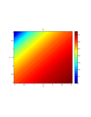
p{c}=22+a+bp{s}=1p{c}formulae-sequencesubscript𝑝𝑐22𝑎𝑏subscript𝑝𝑠1subscript𝑝𝑐p_{\{c\}}=\frac{2}{2+a+b}\qquad p_{\{s\}}=1-p_{\{c\}} (36)
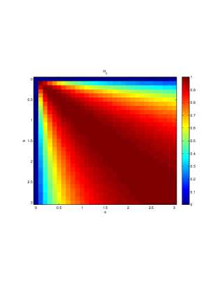
H{s}=K(a,b)H{c}=1formulae-sequencesubscript𝐻𝑠𝐾𝑎𝑏subscript𝐻𝑐1H_{\{s\}}=K(a,b)\qquad H_{\{c\}}=1 (37)

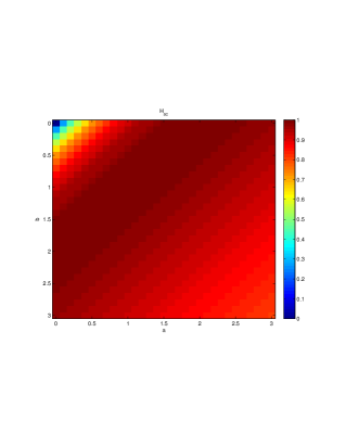
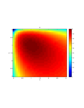
Figures 1 to 4 illustrate probabilities and entropies for this case.

Refer to caption
Figure 1: Heat-map of p{s}subscript𝑝𝑠p_{\{s\}} for the 2-agent case.
Refer to caption
Figure 2: Heat-map of H{s}subscript𝐻𝑠H_{\{s\}} for the 2-agent case.
Refer to caption
Figure 3: Heat-map of H{sc}subscript𝐻𝑠𝑐H_{\{sc\}} for the 2-agent case.
Refer to caption
Figure 4: Heat-map of the overall cash-flow entropy H𝐻H for the 2-agent case. The previous plots are a decomposition of this entropy. We have H=H{sc}+pH{s}+p{c}H{c}𝐻subscript𝐻𝑠𝑐𝑝subscript𝐻𝑠subscript𝑝𝑐subscript𝐻𝑐H=H_{\{sc\}}+pH_{\{s\}}+p_{\{c\}}H_{\{c\}}.

4.2 The three-agent economy

Let us assume stationarity and no savings. The cash-flow matrix is then

[0c21c31c120c32c13c230]delimited-[]0subscriptsuperscript𝑐12subscriptsuperscript𝑐13subscriptsuperscript𝑐210subscriptsuperscript𝑐23subscriptsuperscript𝑐31subscriptsuperscript𝑐320\left[{\begin{array}[]{ccc}0&c^{1}_{2}&c^{1}_{3}\\ c^{2}_{1}&0&c^{2}_{3}\\ c^{3}_{1}&c^{3}_{2}&0\end{array}}\right] (38)

There are two constraints resulting from the stationarity requirement

c1=c1c2=c2formulae-sequencesuperscript𝑐1subscript𝑐1superscript𝑐2subscript𝑐2c^{1}=c_{1}\qquad c^{2}=c_{2} (39)

(this implies c3=c3superscript𝑐3subscript𝑐3c^{3}=c_{3}) and one freedom to “choose the cash denomination” (allowing us to re-scale all values in the cash-flow matrix).

Let us choose the normalization such that the average agent income/spending is 1, i.e.,

c1+c2+c3=3.superscript𝑐1superscript𝑐2superscript𝑐33c^{1}+c^{2}+c^{3}=3. (40)

Furthermore, let us choose the following three parameters for the cash flow matrix

c21c1=ac32c2=bc13c3=k.formulae-sequencesubscriptsuperscript𝑐12superscript𝑐1𝑎formulae-sequencesubscriptsuperscript𝑐23superscript𝑐2𝑏subscriptsuperscript𝑐31superscript𝑐3𝑘\frac{c^{1}_{2}}{c^{1}}=a\qquad\frac{c^{2}_{3}}{c^{2}}=b\qquad\frac{c^{3}_{1}}{c^{3}}=k. (41)

Then the definition of cjsuperscript𝑐𝑗c^{j} implies

c31c1=1ac12c2=1bc23c3=1k.formulae-sequencesubscriptsuperscript𝑐13superscript𝑐11𝑎formulae-sequencesubscriptsuperscript𝑐21superscript𝑐21𝑏subscriptsuperscript𝑐32superscript𝑐31𝑘\frac{c^{1}_{3}}{c^{1}}=1-a\qquad\frac{c^{2}_{1}}{c^{2}}=1-b\qquad\frac{c^{3}_{2}}{c^{3}}=1-k. (42)

Writing down the definitions for c1superscript𝑐1c^{1}, c2superscript𝑐2c^{2} and the mean constraint as a linear system in the cjsuperscript𝑐𝑗c^{j} gives

[c1c23]=[01bka01k111][c1c2c3]delimited-[]superscript𝑐1superscript𝑐23delimited-[]01𝑏𝑘𝑎01𝑘111delimited-[]superscript𝑐1superscript𝑐2superscript𝑐3\left[{\begin{array}[]{c}c^{1}\\ c^{2}\\ 3\end{array}}\right]=\left[{\begin{array}[]{ccc}0&1-b&k\\ a&0&1-k\\ 1&1&1\end{array}}\right]\left[{\begin{array}[]{c}c^{1}\\ c^{2}\\ c^{3}\end{array}}\right] (43)

and hence

[c1c2c3]=B1[003],delimited-[]superscript𝑐1superscript𝑐2superscript𝑐3superscript𝐵1delimited-[]003\left[{\begin{array}[]{c}c^{1}\\ c^{2}\\ c^{3}\end{array}}\right]=B^{-1}\left[{\begin{array}[]{c}0\\ 0\\ 3\end{array}}\right], (44)

where

B=[11bka11k111]𝐵delimited-[]11𝑏𝑘𝑎11𝑘111B=\left[{\begin{array}[]{ccc}-1&1-b&k\\ a&-1&1-k\\ 1&1&1\end{array}}\right] (45)

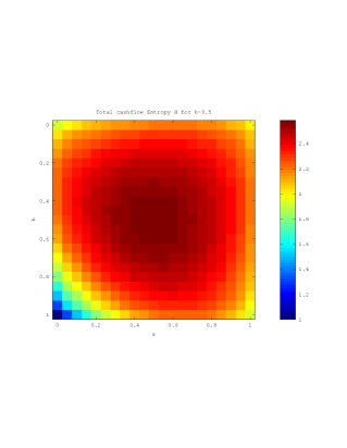
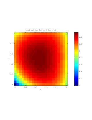
The overall entropy (which is equal to H{c}subscript𝐻𝑐H_{\{c\}} because we excluded savings here) for different values of k𝑘k is presented in the heat plots 5 and 6.
Refer to caption
Figure 5: Heat-map of the overall cash-flow entropy H𝐻H for the 3-agent case with k=0.3𝑘0.3k=0.3.
Refer to caption
Figure 6: Heat-map of the overall cash-flow entropy H𝐻H for the 3-agent case with k=0.5𝑘0.5k=0.5.

To illustrate the identity (28) let us assume a specific case, by fixing the parameters for the cash flow matrix to

a=0.1b=0.3k=0.7.formulae-sequence𝑎0.1formulae-sequence𝑏0.3𝑘0.7a=0.1\quad b=0.3\quad k=0.7. (46)

This corresponds to the cash flow matrix

[00.12351.11180.351600.15070.88370.37870]delimited-[]00.12351.11180.351600.15070.88370.37870\left[\begin{array}[]{ccc}0&0.1235&1.1118\\ 0.3516&0&0.1507\\ 0.8837&0.3787&0\end{array}\right] (47)

The inflow entropies (entropies in each column) are then

H1=0.8617;H2=0.8048;H3=0.5275formulae-sequencesubscript𝐻10.8617formulae-sequencesubscript𝐻20.8048subscript𝐻30.5275H_{1}=0.8617;\quad H_{2}=0.8048;\quad H_{3}=0.5275 (48)

while the outflow entropies (entropies in each row) are then

H1=0.4690;H2=0.8813;H3=0.8813.formulae-sequencesuperscript𝐻10.4690formulae-sequencesuperscript𝐻20.8813superscript𝐻30.8813H^{1}=0.4690;\quad H^{2}=0.8813;\quad H^{3}=0.8813. (49)

Let us define the entropy differentials (inflow minus outflow entropy) Dj=defHjHjsuperscriptdefsubscript𝐷𝑗subscript𝐻𝑗superscript𝐻𝑗D_{j}\stackrel{{\scriptstyle\mbox{\tiny def}}}{{=}}H_{j}-H^{j}

D1=0.3927;D2=0.0765;D3=0.3538formulae-sequencesubscript𝐷10.3927formulae-sequencesubscript𝐷20.0765subscript𝐷30.3538D_{1}=0.3927;\quad D_{2}=-0.0765;\quad D_{3}=-0.3538 (50)

We see that agent 1 is an entropy reducer, while agent 3 is an entropy increaser. Agent 2 is almost entropy neutral. From the cash flow matrix we find the pjsubscript𝑝𝑗p_{j} as

p1=0.4118;p2=0.1674;p3=0.4208.formulae-sequencesubscript𝑝10.4118formulae-sequencesubscript𝑝20.1674subscript𝑝30.4208p_{1}=0.4118;\quad p_{2}=0.1674;\quad p_{3}=0.4208. (51)

Now it is easy to verify that the identity (28) is satisfied. This means that the weighted entropy differentials for any two agents imply the weighted entropy differential for the remaining agent.

5 Conclusion

We presented a formalism linking cash flows to an entropy measure. The measure naturally adopts to sub-goupings of the cash flows and as such produces a number of inequality measures, one of them being the Theil Index.

While the Theil Index is well know, we believe the over all framework we presented is new. It produces inequality measures between all possible groupings of agents and internal inequality measures for each group.

Another interesting result is a kind of overall entropy balance expressed in equation (22) and (28). This essentially says that there must be a balance between entropy increasers (receiving few large cash flow, making many small payments) and decreasers (receiving many small payments and making a few large payments). Whether this can be linked to an “economic energy” is an interesting question which we have not yet addressed. However, one might speculate that entropy increasers (consumers) tend to pay the profit margins received by entropy decreasers (companies).

The formalism presented here does not allow for credit, which is obviously an important factor in the real world. We believe that credit can be incorporated in the formalism and this will be the subject of further research.

Another possible extension is an inclusion of time so that entropy cannot just be measured over one time step, but also over a number of time steps. One way of doing this is to consider discrete times and to treat the same agent at different times as ’different’. This should lead to entropies for payment profiles over time, for example for loans repayed in installments. We hope to be able to explore this more in a seperate paper.

Appendix A Subdivision Identity Example

Let us assume that we have 222 possible outcomes labeled by 111 and 222 with probabilities p1subscript𝑝1p_{1} and p2=1p1subscript𝑝21subscript𝑝1p_{2}=1-p_{1}. The information entropy is then

H=p1log(p1)p2log(p2).𝐻subscript𝑝1subscript𝑝1subscript𝑝2subscript𝑝2H=-p_{1}\log(p_{1})-p_{2}\log(p_{2}). (52)

Now let outcome 222 be the combination of two possible outcomes 212121 and 222222 with probabilities p21subscript𝑝21p_{21} and p22subscript𝑝22p_{22} such that p2=p21+p22subscript𝑝2subscript𝑝21subscript𝑝22p_{2}=p_{21}+p_{22}. We then find for the over-all entropy

H𝐻\displaystyle H =\displaystyle= p1log(p1)p21log(p21)p22log(p22)subscript𝑝1subscript𝑝1subscript𝑝21subscript𝑝21subscript𝑝22subscript𝑝22\displaystyle-p_{1}\log(p_{1})-p_{21}\log(p_{21})-p_{22}\log(p_{22})
=\displaystyle= p1log(p1)subscript𝑝1subscript𝑝1\displaystyle-p_{1}\log(p_{1})
p21log(p2p21p2)p22log(p2p22p2)subscript𝑝21subscript𝑝2subscript𝑝21subscript𝑝2subscript𝑝22subscript𝑝2subscript𝑝22subscript𝑝2\displaystyle\quad-p_{21}\log\left(p_{2}\frac{p_{21}}{p_{2}}\right)-p_{22}\log\left(p_{2}\frac{p_{22}}{p_{2}}\right)
=\displaystyle= p1log(p1)p2log(p2)subscript𝑝1subscript𝑝1subscript𝑝2subscript𝑝2\displaystyle-p_{1}\log(p_{1})-p_{2}\log(p_{2})
+p2[p21p2log(p21p2)p22p2log(p22p2)]subscript𝑝2delimited-[]subscript𝑝21subscript𝑝2subscript𝑝21subscript𝑝2subscript𝑝22subscript𝑝2subscript𝑝22subscript𝑝2\displaystyle\quad+p_{2}\left[-\frac{p_{21}}{p_{2}}\log\left(\frac{p_{21}}{p_{2}}\right)-\frac{p_{22}}{p_{2}}\log\left(\frac{p_{22}}{p_{2}}\right)\right]

The first two terms are the information entropy for outcome 111 and the aggregate outcome 222. The second term then adds the internal information entropy resulting from the sub-division of outcome 222, which is the weighted information entropy of the probabilities conditional on the knowledge that outcome 222 is true.

Above derivation can be generalized in an obvious way to arrive at (5).

References

  • [1]
  • [2] Jaynes E T, Bretthorst L G (2003), Probability Theory: The Logic of Science, Cambridge University Press, Cambridge
  • [3] Theil H (1967), Economics and Information Theory, North Holland Publishing Company, Amsterdam
  • [4] Shorrocks A F (1980), ‘The Class of Additive Decomposable Inequality Measures’, Econometrica Vol 48 No 3, 613-25