Description of and at small using a collinearly-improved BFKL resummation
Abstract
We present a detailed description of the and dependence of the structure functions and as extracted from the Deep Inelastic Scattering data at HERA in the small Bjorken region. Making use of a collinearly-improved BFKL equation at next-to-leading order and a treatment of the running of the coupling using non-Abelian physical renormalization together with the BLM scale choice allows us to reach low values of . We also provide some predictions for future lepton-hadron colliders.
1 Introduction & review of our framework
Recently, in [1], we calculated the effective slope for the structure function when parameterized as at low Bjorken , which ranges from to when moving from low to high values of . The importance of a correct understanding of the HERA data using perturbative QCD techniques, in particular for the physics program at the Large Hadron Collider (LHC), has been largely discussed in the literature (see, e.g., Ref. [2]).
In this Letter we will not only further investigate the and dependence of but also study in detail the longitudinal structure function . As in [1] we will explore the small region using the next-to-leading order (NLO) [3] BFKL [4] equation with collinear improvements, together with optimal renormalization schemes.
Let us first briefly review our formulæ [1]. At small , with being the squared center-of-mass energy, we can apply high energy factorization and write the structure functions , as (note that the integrations take place in the transverse space with )
| (1) |
is the non-perturbative proton impact factor which we model using
| (2) |
where we have introduced two free parameters and a normalization. is the impact factor associated to the photon which in [1] we treated at leading-order (LO), i.e.
| (3) |
where
| (4) |
, , , and the strong coupling is fixed at the renormalization scale . In the present work we will also use the kinematically improved impact factors proposed in [5, 6], which include part of the higher order corrections by considering exact gluon kinematics. Its implementation requires to replace the functions by where
| (5) |
and , with
| (6) |
is the logarithmic derivative of the Euler Gamma function and , while is the Mellin variable conjugate to in the definition of the gluon Green function , see Eq. (7) below. The main difference between these impact factors is that the LO ones roughly double the value of their kinematically improved counterparts in the region with small , while being very similar for .
The gluon Green function can be written in the form
| (7) |
with . The collinearly improved BFKL kernel as introduced in eq. (7) is an operator consisting of a diagonal (scale invariant) piece with eigenvalue
| (8) |
where , and , plus a term proportional to which contains the running coupling corrections of the NLO kernel [7]:
| (9) |
The precise form of the NLO kernel can be found in [1]. The resummation of collinear logarithms of order and beyond is realized by the term [8, 9, 1]
| (10) |
Our final expression for the structure functions reads
where and can be found in [1]. For the kinematical improved version of we replace by .
In Eq. (1) the scale of the running of the coupling has been set to . Building on the work of [10] we found in [1] that in order to obtain a good description of the dependence of the effective intercept of , , for , it is very useful to operate with non-Abelian physical renormalization schemes using the Brodsky-Lepage-Mackenzie (BLM) optimal scale setting [11] with the momentum space (MOM) physical renormalization scheme [12]. For technical details on our precise implementation we refer the reader to [1] (see also [13] for a review on the subject and [14] for a related work). More qualitatively, in these schemes the pieces of the NLO BFKL kernel proportional to are absorbed in a new definition of the running coupling in order to remove the infrared renormalon ambiguity. Once this is done, the residual scheme dependence in this framework is very small. We also found it convenient [1] to introduce, in order to describe the data with small , an analytic parametrization of the running coupling in the infrared proposed in [15].
2 Comparison to DIS experimental data
In the following we compare our results with the experimental data for and .
2.1
Let us first compare the result obtained in [1] for the logarithmic derivative using Eq. (1) with a LO photon impact factor and our new calculation using the kinematically improved one. In Fig. 1 we present our results with the values of our best fits for both types of impact factors and compare them with the H1-ZEUS combined data [16] for . The values of the parameters defining the proton impact factor in (2) and the position of the (regularized) Landau pole (we use ) for the strong coupling are , GeV, GeV for the LO order case and , GeV, GeV for the kinematically improved (note that the normalization does not contribute to this quantity).
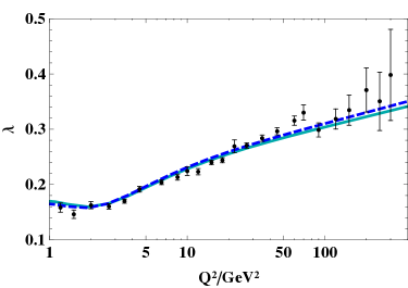
The LO impact factor generates lower values than the kinematically improved one in the high region and slightly higher ones when . It is interesting to see how the approach presented here allows for a good description of the data in a very wide range of , not only for high values, where the experimental uncertainties are larger, but also in the non-perturbative regions due to our treatment of the running of the coupling.
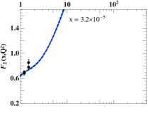
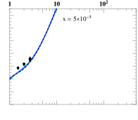
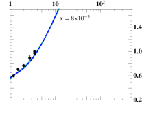
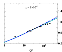
Encouraged by these positive results we now turn to investigate more differential distributions. We select data with fixed values of and compare the dependence of our theoretical predictions with them, now fixing the normalization for the LO impact factor to and for the kinematically improved. Our results are presented in Fig. 2.
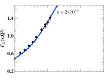
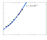
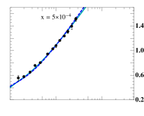
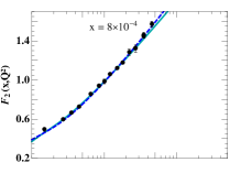
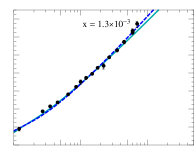
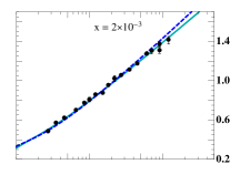
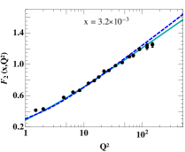
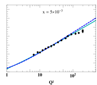
The equivalent comparison to data, this time fixing and looking into the evolution in the variable, is shown in Fig. 3.
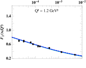
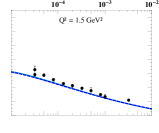
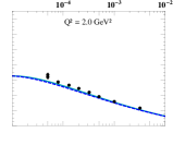
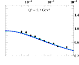
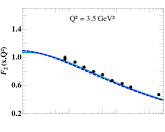
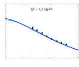
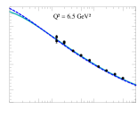
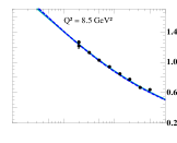
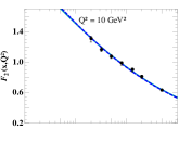
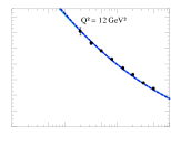
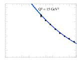
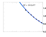
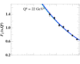
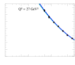
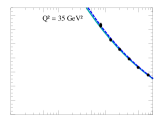
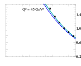
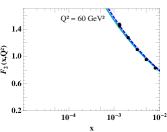
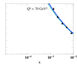
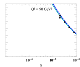
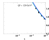
We observe that our predictions give a very accurate description of the data for both types of impact factors.
Let us remark that the values for the parameters in this fit are in syntony with the theoretical expectations for the proton impact factor since is very similar to the confinement scale and the value of sets the maximal contribution from the impact factor also in that region. This is reasonable given that the proton has a large transverse size.
2.2
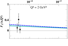
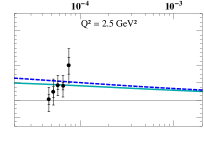
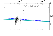
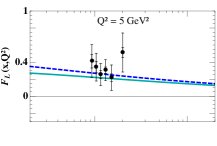
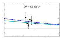
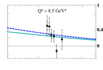
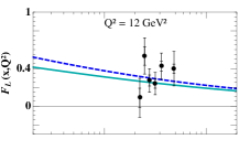
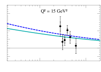
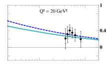
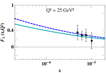
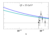
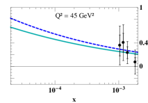
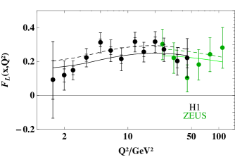
The longitudinal structure function is an interesting observable which is very sensitive to the gluon content of the proton. We will now present our predictions for using the best values for the parameters previously obtained in the fit of . We will see that the agreement with the data is very good. First, is fixed and the dependence is investigated in Fig. 4. The experimental data have been taken from [18]. To present the dependence it is convenient to calculate, for each bin in , the average value of , see Fig. 5. In some sense this is a similar plot to the one previously presented for in the analysis and we can see that the effect of using different types of impact factors is to generate a global shift in the normalization. Again we note that we have an accurate description of the transition from high to low , which was one of the main targets of our work.
3 Predictions for future colliders
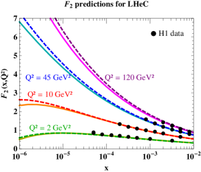
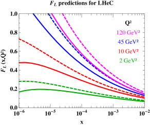
While our predictions for the structure functions are in agreement with the data from the HERA collider experiments H1 and ZEUS, these observables are too inclusive to provide unambiguous evidence for BFKL evolution (for other recent studies in this context see [17]). Comparable in quality fits can be obtained by both DGLAP evolution and saturation models, see e.g. [18, 19]. In order to distinguish among different parton evolution pictures new collider experiments are needed, such as the proposed Electron-Ion-Collider (EIC) at BNL/JLab (USA) [20] and the Large Hadron Electron Collider (LHeC) at CERN (Switzerland) [21], which will be able to measure both and at unprecedented small values of Bjorken . In Fig. 6 we present two studies with our predictions for and down to values of .
4 Conclusions
We have presented an application of the BFKL resummation program to the description of the and dependence of structure functions as extracted from Deep Inelastic Scattering data at HERA. We have also provided some predictions for these observables at future colliders. In order to obtain the correct dependence on the virtuality of the photon at high values of the scattering energy, we have included in the BFKL kernel the main collinear contributions to all orders. We have also used optimal renormalization and an analytic running coupling in the infrared in order to accurately describe the regions of low . Our next task will be to use these parameterizations to describe more exclusive observables, such as heavy quark and multi-jet production, at the Large Hadron Collider at CERN.
Acknowledgments
We acknowledge partial support from the European Comission under contract LHCPhenoNet (PITN-GA-2010-264564), the Comunidad de Madrid through HEPHACOS S2009/ESP-1473, and MICINN (FPA2010-17747) and Spanish MINECOs Centro de Excelencia Severo Ochoa Programme under grant SEV-2012-0249. M.H. acknowledges support by the U.S. Department of Energy under contract number DE-AC02-98CH10886 and a BNL “Laboratory Directed Research and Development” grant (LDRD 12-034).
References
- [1] M. Hentschinski, A. Sabio Vera and C. Salas, arXiv:1209.1353 [hep-ph].
- [2] M. Dobbs et al., hep-ph/0403100. M. Dittmar et al., hep-ph/0511119. S. Alekhin, et al., hep-ph/0601012. J. R. Andersen et al. [Small x Collaboration], Eur. Phys. J. C 48 (2006) 53 [hep-ph/0604189]. H. Jung et al., arXiv:0809.0549 [hep-ph]. Z. J. Ajaltouni et al., arXiv:0903.3861 [hep-ph].
- [3] V. S. Fadin, L. N. Lipatov, Phys. Lett. B 429 (1998) 127, M. Ciafaloni, G. Camici, Phys. Lett. B 430 (1998) 349.
- [4] L. N. Lipatov, Sov. J. Nucl. Phys. 23 (1976) 338, E. A. Kuraev, L. N. Lipatov, V. S. Fadin, Phys. Lett. B 60 (1975) 50, Sov. Phys. JETP 44 (1976) 443, Sov. Phys. JETP 45 (1977) 199. I. I. Balitsky, L. N. Lipatov, Sov. J. Nucl. Phys. 28 (1978) 822.
- [5] J. Kwiecinski, A. D. Martin and A. M. Stasto, Phys. Rev. D 56, 3991 (1997) [hep-ph/9703445].
- [6] A. Bialas, H. Navelet and R. B. Peschanski, Nucl. Phys. B 603, 218 (2001) [hep-ph/0101179].
- [7] A. Sabio Vera, F. Schwennsen, Phys. Rev. D 77 (2008) 014001 [arXiv:0708.0549 [hep-ph]], Nucl. Phys. B 776 (2007) 170 [hep-ph/0702158 [HEP-PH]], A. Sabio Vera, Nucl. Phys. B 746 (2006) 1 [hep-ph/0602250], F. Caporale, A. Papa, A. Sabio Vera, Eur. Phys. J. C 53 (2008) 525 [arXiv:0707.4100 [hep-ph]].
- [8] G. P. Salam, JHEP 9807 (1998) 019 [hep-ph/9806482].
- [9] A. Sabio Vera, Nucl. Phys. B 722 (2005) 65 [hep-ph/0505128].
- [10] S. J. Brodsky, V. S. Fadin, V. T. Kim, L. N. Lipatov and G. B. Pivovarov, JETP Lett. 70 (1999) 155 [hep-ph/9901229], JETP Lett. 76 (2002) 249 [Pisma Zh. Eksp. Teor. Fiz. 76 (2002) 306] [hep-ph/0207297].
- [11] S. J. Brodsky, G. P. Lepage and P. B. Mackenzie, Phys. Rev. D 28 (1983) 228.
- [12] W. Celmaster and R. J. Gonsalves, Phys. Rev. D 20 (1979) 1420, Phys. Rev. Lett. 42 (1979) 1435, P. Pascual and R. Tarrach, Nucl. Phys. B 174 (1980) 123 [Erratum-ibid. B 181 (1981) 546].
- [13] S. J. Brodsky and L. Di Giustino, Phys. Rev. D 86 (2012) 085026 [arXiv:1107.0338 [hep-ph]].
- [14] M. Angioni, G. Chachamis, J. D. Madrigal and A. Sabio Vera, Phys. Rev. Lett. 107 (2011) 191601 [arXiv:1106.6172 [hep-th]].
- [15] B. R. Webber, JHEP 9810 (1998) 012. [hep-ph/9805484].
- [16] F. D. Aaron et al. [H1 and ZEUS Collaboration], JHEP 1001 (2010) 109 [arXiv:0911.0884 [hep-ex]].
- [17] H. Kowalski, L. N. Lipatov, D. A. Ross and G. Watt, Eur. Phys. J. C 70 (2010) 983 [arXiv:1005.0355 [hep-ph]], H. Kowalski, L. N. Lipatov and D. A. Ross, arXiv:1109.0432 [hep-ph], arXiv:1205.6713 [hep-ph].
- [18] F. D. Aaron et al. [ H1 Collaboration], Eur. Phys. J. C 71, 1579 (2011) [arXiv:1012.4355 [hep-ex]].
- [19] S. Chekanov et al. [ZEUS Collaboration], Phys. Lett. B 682, 8 (2009) [arXiv:0904.1092 [hep-ex]].
- [20] A. Deshpande et al., arXiv:1212.1701 [nucl-ex], D. Boer et al., arXiv:1108.1713 [nucl-th].
- [21] J. L. Abelleira Fernandez et al. [LHeC Study Group Collaboration], J. Phys. G 39, 075001 (2012) [arXiv:1206.2913 [physics.acc-ph]].