Web: ]http://www.iop.kiev.ua/ obraun

Size scaling of static friction

Abstract

Sliding friction across a thin soft lubricant film typically occurs by stick-slip, the lubricant fully solidifying at stick, yielding and flowing at slip. The static friction force per unit area preceding slip is known from molecular dynamics (MD) simulations to decrease with increasing contact area. That makes the large-size fate of stick-slip unclear and unknown; its possible vanishing is important as it would herald smooth sliding with a dramatic drop of kinetic friction at large size. Here we formulate a scaling law of the static friction force, which for a soft lubricant is predicted to decrease as $f_{m}+\Delta f/A^{\gamma}$ for increasing contact area $A$, with $\gamma>0$. Our main finding is that the value of $f_{m}$, controlling the survival of stick-slip at large size, can be evaluated by simulations of comparably small size. MD simulations of soft lubricant sliding are presented, which verify this theory.

Boundary friction of sliding crystal surfaces across atomically thin solid or nearly solid lubricant layers, of considerable conceptual and practical importance, also constitutes an open physics problem, because the uncertain occurrence of stick-slip makes the prediction of the overall frictional regime – stick-slip or smooth sliding – rather uncertain Pbook ; BN2006 . While for hard solid lubricants the answer is known, namely stick-slip for commensurate and crystallographically aligned interfaces or smooth sliding for lattice mismatched/misaligned interfaces note0 , it is not so for soft solid lubricants. The latter, with shearing occuring inside the lubricant rather than at the surface/lubricant interface, represent the commonest case, realized at room temperature in e.g. commercial machine oils confined in between metallic surfaces. The possibility of smooth sliding would be especially relevant, because of the accompanying large drop of kinetic friction, often a very desirable outcome. The crucial controlling quantity is the magnitude of static friction $f_{s}$ – the maximum pulling force reached before slip. So long as $f_{s}$ is finite there will be stick-slip; when $f_{s}$ drops to zero, there can only be smooth sliding. Realistic molecular dynamics (MD) simulations of lubricants confined between atomically flat surfaces generally indicate that stick-slip prevails for soft lubricants, with consequently high kinetic friction. However, while in smooth sliding the kinetic friction per unit area is essentially size independent, its static counterpart $f_{s}$ may decrease with increasing contact area $A$ Pbook ; BN2006 . Despite the increased computer power, the simulated system sizes Jagla02 ; Luan04 ; Luan05 ; Vanossi13 are still far too small to establish conclusively whether in the limit of mesoscopically large size the static friction will remain finite, and stick-slip will survive with large kinetic friction, or if it will vanish so that smooth sliding and low dynamic friction will eventually prevail. The time-honored approach borrowed from equilibrium statistical mechanics to this type of question is finite-size scaling binder_somebook . One can for example double repeatedly the size of the simulation cell and compare the change in the results with some analytically predicted size dependence from theory. Given a good scaling prediction, a few simulated sizes are often sufficient to establish the large-size limit with reasonable accuracy, and in particular whether static friction will drop to zero and stick-slip will disappear, or not.

In this Letter we solve this question, first by deriving a size scaling law for static friction, and then showing that it fits realistic MD simulations yielding a well defined answer. Our end result is that (i) the predicted drop of the size-dependent part of the static friction per atom $f_{s}$ is inversely proportional to the linear size of the contact (i.e. to $A^{1/2}$), but that (ii) its predicted large-size limit is nonzero, so that stick-slip will generally survive in soft solid boundary lubrication.

Scaling theory. To start off the theory, we inspect first the dynamics of previous MD simulations of sliding over soft solid lubricants BN2006 ; BP2001 ; BraunManini11 . These simulations indicate, very reasonably, that unlike hard lubricants where sliding occurs at the interfaces, plastic motion within the soft lubricant nucleates typically at some weak point well inside the lubricant film, such as a point defect, a dislocation, a local incommensurability, etc. (similarly to the “weakest-link hypothesis” of fracture mechanics, e.g., see Refs. George52 ; MSNASZ2012 and references therein). The static friction force $f_{s}$ (per substrate atom, i.e. $f_{s}=\sigma_{s}L_{x}L_{y}/N_{s}$, where $\sigma_{s}$ is the shear stress, $L_{x}$ and $L_{y}$ are the sides of the rectangular simulation cell, and $N_{s}$ is the number of substrate surface atoms) depends on the given initial (frozen) configuration. For a given size $A=L_{x}\times L_{y}$ of the simulation cell, different realizations of the initial configuration will give different $f_{s}$ values $f_{s\,1}<f_{s\,2}<...$, where a given value $f_{s\,i}$ is realized with probability $p_{i}^{(A)}$. Now suppose we double the simulation cell. Slip-motion will again start at the weakest point wherever it is, in either half of the doubled cell. Assuming that the new (larger) contact does not develop new thresholds, the probability that the doubled cell fails at threshold $f_{s\,i}$ equals the sum of the probability that failure occurs precisely at this threshold $f_{s\,i}$ in both halfs plus the probability that in one half the threshold is $f_{s\,i}$ and in the other half it is some larger $f_{s\,j}$:

$$p_{i}^{(2A)}=\left(p_{i}^{(A)}\right)^{2}+2p_{i}^{(A)}\sum_{j>i}p_{j}^{(A)}.$$ (1)

The factor 2 accounts for the the two symmetric realizations of $f_{s\,j}$ and $f_{s\,i}$ in the two halves.

By iteration of Eq. (1), we can find the probability $p_{i}^{(\Lambda A)}$ for larger and larger cell size $\Lambda A\equiv 2^{n}A$, with $n=0,1,\ldots$ Given the resulting distribution, one can calculate the average static threshold for the $\Lambda A$ cell by

$$\bar{f}_{s}(\Lambda)=\sum_{i}p_{i}^{(\Lambda A)}f_{si}\,.$$ (2)

To illustrate this approach, consider the simple instructive example where only two thresholds $f_{s\,1}=f_{m}$ and $f_{s\,2}=f_{m}+\Delta f>f_{m}$ occur, with probabilities $p_{1}$ and $p_{2}$. For the doubled cell, we have four possible thresholds realizations: $(f_{s\,1},f_{s\,1})$ with probability $p_{1}^{2}$, $(f_{s\,1},f_{s\,2})$ with probability $p_{1}p_{2}$, $(f_{s\,2},f_{s\,1})$ with probability $p_{2}p_{1}$, and $(f_{s\,2},f_{s\,2})$ with probability $p_{2}^{2}$. Accordingly, the doubled cell fails at the lower threshold with probability $p_{1}^{2}+2p_{1}p_{2}$, and at the upper threshold with probability $p_{2}^{2}$. Indicate with $p_{1}^{(A)}=1-\alpha$ and $p_{2}^{(A)}=\alpha<1$. The iteration chain is $p_{2}^{(2\Lambda A)}=\left[p_{2}^{(\Lambda A)}\right]^{2}$, with solution $p_{2}^{(\Lambda A)}=\alpha^{\Lambda}$, and thus $p_{1}^{(\Lambda A)}=1-\alpha^{\Lambda}$. Accordingly, the average static friction approaches the minimum threshold $f_{m}$ exponentially in $\Lambda$:

$$\bar{f}_{s}(\Lambda)-f_{m}=\alpha^{\Lambda}\Delta f=e^{\Lambda\ln\alpha}\Delta f\,.$$ (3)

Figure 1: (color online) Iteration of Eq. (4) starting from a sawtooth initial distribution $P_{c}^{(A)}(f)=2\,f\,\theta(f)\,\theta(1-f)$, where $\theta(x)$ is the Heaviside step function. Inset (a) shows successive iterations of $P_{c}^{(\Lambda A)}(f)$ for $\Lambda=1,2,4,8,\dots$ Inset (b) displays the scaled distribution $\Lambda^{-\gamma}P_{c}^{(\Lambda A)}(\Lambda^{-\gamma}f)$ compared to the infinite-size solution (10). The main graph shows the average static friction $\bar{f}$ excess (above the minimum $f_{m}$) as a function of contact size.

When we replace the discrete thresholds $f_{s\,i}$ with a more realistic continuous distribution with probability $P_{c}^{(A)}(f_{s})$, the first, quadratic, contribution in Eq. (1) can be neglected, and the iteration equation takes the form

$$P_{c}^{(2A)}(f_{s})=2P_{c}^{(A)}(f_{s})\times\int_{f_{s}}^{\infty}P_{c}^{(A)}(f_{s}^{\prime})\,df_{s}^{\prime}\,.$$ (4)

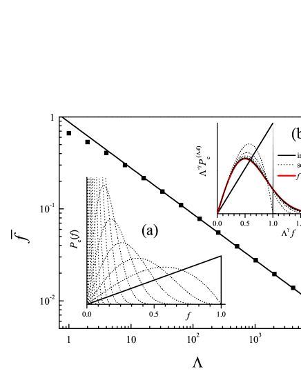
Figure 1(a) illustrates an example of the numerical iteration of this equation. Simulations suggest that for large $\Lambda$ the distribution $P_{c}^{(\Lambda A)}(f_{s})$ tends to approach some universal shape, with little dependency on the small-size distribution $P_{c}^{(A)}(f_{s})$, once it is rescaled appropriately. A similar scaling behavior was proven for the strain distributions of the (related) fiber-bundle models Newman91 ; Smalley85 ; Newman94 ; Newman01 ; note1 . In these models the conditions for the emergence of a critical point, i.e. a finite stress in the large-scale limit, were investigated under the assumption of a nonzero single-fiber breaking probability for arbitrarily small stress. Here instead we consider that more generally the minimal contact (“single fiber”) distribution of unpinning forces $f_{s}$ can start off at a minimum $f_{m}$ which can be nonzero. Iteration of Eq. (4) guarantees that for any contact size $\Lambda A$ the distribution $P_{c}^{(\Lambda A)}(f_{s})$ vanishes below the same $f_{m}$ as $P_{c}^{(A)}(f_{s})$: scaling preserves $f_{m}$. To address the scaling of the distribution above $f_{m}$, it is convenient to introduce $f=f_{s}-f_{m}$. Let us assume that at large $\Lambda$ the normalized probability distribution scales as

$$P_{c}^{(2\Lambda A)}(f)=aP_{c}^{(\Lambda A)}(af)\,,$$ (5)

where $a>1$ is a constant. By substituting Eq. (5) into Eq. (4), for the large-size distribution $g(f)=\lim_{\Lambda\to\infty}\Lambda^{-\gamma}P_{c}^{(\Lambda A)}\left(\Lambda^{-\gamma}\,f\right)$, with $\gamma=\log_{2}a$, we obtain the following equation:

$$a\,g(af)=2g(f)\int_{f}^{\infty}g(f^{\prime})\,df^{\prime},$$ (6)

or

$$\frac{a\,g(af)}{g(f)}=2\int_{f}^{\infty}g(f^{\prime})\,df^{\prime}.$$ (7)

Differentiating both sides with respect to $f$, we get

$$a^{2}g^{\prime}(af)\,g(f)-a\,g(af)\,g^{\prime}(f)+2g^{3}(f)=0\,.$$ (8)

The solutions of this equation depend on a single feature of the distribution $g(f)$, namely its small-$f$ behavior. More precisely, assuming that $g(f)=\sum_{k=k_{0}}c_{k}f^{k}$, with $k_{0}>-1$, we have that

$$a = 2^{\gamma}\qquad{\rm with}\ \gamma=(1+k_{0})^{-1}\,,$$ (9)

$$g(f) = c_{k_{0}}f^{k_{0}}\exp\left(-\frac{c_{k_{0}}f^{1+k_{0}}}{1+k_{0}}\right)$$ (10)

solve Eq. (8). Figure 1(b) demonstrates the approach of the scaled distributions to the function $g(f)=f\,\exp(-f^{2}/2)$ (with $a=\sqrt{2}$) obtained by starting off with an initial distribution $P_{c}^{(A)}(f)=2\,f\,\theta(f)\,\theta(1-f)$, i.e. with $k_{0}=1$, $c_{1}=2$.

The scaling theory makes the following predictions: (i) as scaling preserves $f_{m}$, it is possible to predict the minimum threshold $f_{m}$ from an evaluation of $P_{c}^{(A)}(f)$ at the smallest contact size; (ii) the iteration defined by Eq. (4) preserves the leading term in the $f$ power expansion of $P_{c}^{(A)}(f)$ above $f_{m}$; (iii) regardless of the overall shape of the small-size threshold distribution, for large size the distribution acquires the “universal” shape of Eq. (10); (iv) its width $\Delta f^{(\Lambda A)}$ scales down as an inverse power law of $\Lambda$; (v) this power law is dictated uniquely by the leading power law with which the arbitrary-size threshold distribution behaves for $f_{s}$ near $f_{m}$; (v) as $\Lambda$ increases, the average friction force $\bar{f}_{s}$ approaches $f_{m}$ according to the law

$$\bar{f}_{s}(\Lambda)-f_{m}\simeq\left[\bar{f}_{s}(\Lambda=1)-f_{m}\right]\Lambda^{-\gamma}\,.$$ (11)

In the example of Fig. 1, this relation yields a mean excess static friction scaling as the inverse square root of size $\bar{f}_{s}-f_{m}\propto\Lambda^{-1/2}$.

Figure 2: (color online) (a) The time evolution of the spring force during a segment of the simulated stick-slip dynamics of the $12\times 11$ substrate model driven at speed 0.01 n.u., with an applied load of 0.1 n.u. per rigid substrate atom; circles mark the stick-to-slip transitions where the individual static-friction thresholds $f_{si}$ are extracted. (b) The probability distribution of the static-friction thresholds $P_{c}^{(A)}(f_{s})$ as estimated by a histogram of the $f_{si}$ values. A dotted line marks the mean value $\bar{f}_{s}$, and an arrow marks the estimated $f_{m}$.

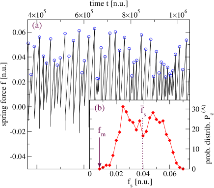
Simulation. To validate our prediction with MD simulations, we use our previously developed model BN2006 ; BP2001 ; BraunManini11 . Each of the two substrates is modeled by two atomic layers, one rigid and one deformable. In the minimum size simulation of contact area $A$, these substrates are composed by $12\times 11$ atoms arranged in a square lattice. The space between the substrates is filled by three incomplete layers of lubricant atoms (to prevent crystallization of the lubricant, we put approximately 90% of the atoms which would complete 3 perfect monolayers). All atoms interact according to the Lennard-Jones (LJ) potential. The strength of the lubricant-lubricant interaction is $V_{ll}=1/9$ (in dimensionless “natural” units, n.u., defined for example in Refs. BP2001 ; BN2006 ), while the lubricant-substrate interaction is much stronger, $V_{sl}=1/3$. The equilibrium distance of the LJ lubricant-lubricant interatomic potential is $r_{ll}/a_{s}=3.95/3$ (i.e., the solid lubricant is incommensurate with the substrate). These parameters correspond to a soft lubricant. Once the thin soft lubricant film is interposed between the sliders, sliding takes place inside the lubricant (as opposed to hard lubricants where the sliding would take place at the interfaces) and the film melts during sliding, realizing the melting-freezing mechanism of stick-slip motion. The bottom substrate is kept fixed, while the rigid top slider layer is pressed with a load of $0.1$ n.u. per substrate atom (representing a pressure in the order $100$ MPa if the model represented a noble gas solid lubricant between metal surfaces) and driven through a spring of elastic constant $k=3\times 10^{-4}$ n.u. per atom with a velocity $v$. We carry out simulations at driving velocities $v=3\times 10^{-3}\div 3\times 10^{-2}$ n.u. These velocities are sufficiently small that the system exhibits stick-slip motion, as illustrated in Fig. 2(a). We carry out runs of duration exceeding $10^{7}$ n.u. for the smallest-size system ($12\times 11$), representing $\Lambda=1$. By extracting the “static friction” thresholds $f_{si}$ marked by circles in Fig. 2(a) in correspondence to the peaks in $f(t)$ preceding each slip event, we obtain a set $\{f_{si}\}$ sampling the probability distribution $P_{c}^{(A)}(f_{s})$. We evaluate this distribution by means of a histogram of 1063 thresholds obtained during a long run, and shown in Fig. 2(b). Although the detailed behavior near the minimum threshold $f_{m}$ is naturally affected by limited statistics, the data are consistent with a distribution staring off at $f_{m}\simeq 0.0075$, with an approximately linear slope ($k_{0}=1$), which produces an exponent $\gamma=1/2$. From the threshold distribution $P_{c}^{(A)}(f_{s})$ we extract the mean value $\bar{f}_{s}=0.0397$, marked by a dotted line in Fig. 2(b).

Figure 3: (color online) The average static friction force per substrate atom as a function of the system size, as obtained from molecular dynamics simulations in the same conditions as those of Fig. 2, with several sizes multiple of the $12\times 11$ substrate model which is represented by the first $\Lambda=1$ point in figure. The solid line shows the scaling law, Eq. (11). Inset: log-log scale. The dashed line marks $f_{m}$, estimated by the lowest observed slip threshold in all simulations of all sizes.

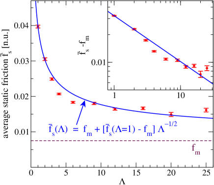
Having thus characterized the small-area sliding behavior, we proceed to increase the area in order to track the size-induced changes. The cell is successively increased to $\Lambda=2=2\times 1$, $3=3\times 1$, $4=2\times 2$, $6=3\times 2$, $9=3\times 3$, $12=4\times 3$, $16=4\times 4$, $20=5\times 4$, and $25=5\times 5$. The results are presented in Fig. 3. As expected, the average static friction decreases with system size. As was noted, it would not be feasible to extract a large-size limit in the absence of a scaling law. We find that scaling law (11) with $\gamma=1/2$ fits the simulation results with reasonable accuracy. The static friction tends to a finite large-size value $f_{m}>0$, and therefore stick-slip will survive at macroscopic size.

Discussion. We just arrived at the conclusion that once $f_{m}$ starts off nonzero, $f_{s}$ will converge to $f_{m}>0$ and static friction will not disappear in the large-size limit. One should however not jump to the conclusion that once the static friction threshold distribution starts from zero, $f_{m}=0$, the amplitude of stick-slip jumps of $f(t)$ will drop to zero, and stick-slip friction will necessarily disappear in the limit of large contact area. There are two reasons why this is not generally true. The first reason resides in statics, and follows from elasticity of the substrate. The size $\lambda_{c}$ of a domain that can be considered as rigid and slides as a whole, is determined by the elastic correlation length CN1998 ; BPST2012 . Therefore, the average static friction force should reach a plateau for sizes $L\simeq A^{1/2}\gtrsim\lambda_{c}$ note2 . The second reason follows from kinetics. When the sliding motion starts off at some weak contact site, it may either die off, or spread over the whole interface with some speed $c$. This process takes a finite time $\tau\sim L/c$. If at a given driving velocity $v$, $\tau$ is of order or larger then the time between successive slips $\tau_{ss}\sim f_{s}(L)/(kv)$, then the local sliding initiated by this weak contact will lose its role and effectiveness for all sizes $L>\lambda_{d}$, where $\lambda_{d}=(c/v)\,f_{s}(\lambda_{d})/k$, hence the static friction will saturate rather than decrease further to $f_{m}$ as predicted by the scaling theory Eq. (11).

This leads us to ask more generally what is lost in the scaling approach? We assumed that the doubled cell has the same set of thresholds $\{f_{si}\}$ as the original one. Yet a larger cell may develop new collective excitations, e.g., a dislocation loop of a size $>L$. However, if the original cell $A$ is large enough, we may still safely extrapolate its distribution to a mesoscopic size, where the master equation approach BP2008 is applicable.

Another situation where a different behaviour is expected is the Aubry incommensurate superlubric state, which has zero static friction threshold in the infinite system BKbook . That state, corresponding to $f_{m}=0$ in our theory, occurs preferentially for hard lubricants whose interior does not develop a shear band, and which do not melt during sliding.

Experimentally, the scaling behavior predicted here could be probed by comparing friction-force microscopy realizations with tips of different curvature radii Meyer98 ; Schwarz97 sliding on a surface covered by a lubricant close to its melting points, e.g. an octamethylcyclotetrasiloxan or an ionic liquid at room temperature, or a noble-gas layer at a cryogenic temperature. The technological bottomline lesson, finally, is that stick-slip could be attenuated by reducing the smallest threshold force, for example by promoting extra defects in the lubricant film by additives or other means.

Acknowledgments. We thank A. Vanossi and M. Urbakh for helpful discussions. O.M.B. was supported in part by grants from the Cariplo Foundation managed by the Landau Network – Centro Volta, whose contribution is gratefully acknowledged. He also thanks ICTP and SISSA (Trieste), and the University of Milan, for hospitality during this project. E.T. acknowledges support by SINERGIA Project CRSII2 136287/1.

References

- (1) B.N.J. Persson, Sliding friction: Physical principles and applications (Springer-Verlag, Berlin, 1998).
- (2) O.M. Braun and A.G. Naumovets, Surf. Sci. Reports 60, 79 (2006).
- (3) Static friction can also arise for stiff (although not rigid) disordered surfaces, via the mechanism discussed in Ref. CN1998 .
- (4) E. A. Jagla, Phys. Rev. Lett. 88, 245504 (2002).
- (5) B. Luan and M. O. Robbins, Phys. Rev. Lett. 93, 036105 (2004).
- (6) B.Q Luan and M.O. Robbins, Nature (London) 435, 929 (2005).
- (7) A. Vanossi, A. Benassi, N. Varini, and E. Tosatti, Phys. Rev. B 87, 045412 (2013).
- (8) K. Binder and D.W. Heermann, Monte Carlo simulation in statistical physics (Springer-Verlag, Berlin, 2002).
- (9) O.M. Braun and M. Peyrard, Phys. Rev. E63, 046110 (2001).
- (10) O.M. Braun and N. Manini, Phys. Rev. E83, 021601 (2011).
- (11) W. George, Ind. Eng. Chem. 44, 1328 (1952).
- (12) C. Manzato, A. Shekhawat, P.K.V.V. Nukala, M.J. Alava, J.P. Sethna, and S. Zapperi, Phys. Rev. Lett. 108, 065504 (2012).
- (13) W.I. Newman and A.M. Gabrielov, Int. J. Fracture 50, 1 (1991).
- (14) R.F. Smalley, D.L. Turcotte, and S.A. Solla, J. Geophys. Res. 90, 1894 (1985).
- (15) W.I. Newman, A.M. Gabrielov, T.A. Durand, S.L. Phoenix, and D.L. Turcotte, Physica D 77, 200 (1994).
- (16) W.I. Newman and S.L. Phoenix, Phys. Rev. E63, 021507 (2001).
- (17) In the fiber-bundle model Newman91 ; Smalley85 ; Newman94 ; Newman01 , the failing of one fibre leads to a load redistribution over neighboring fibres which then could fail too; the complete failing (“sliding”) occurs when all fibres fail. In our model of frictional interface we assume, according to MD simulation, that sliding occurs when any of the contacts breaks (melts), and the driving-induced melting spreads across the interface leading to overall sliding.
- (18) C. Caroli and Ph. Nozieres, Eur. Phys. J. B 4, 233 (1998).
- (19) O.M. Braun, M. Peyrard, D.V. Stryzheus, and E. Tosatti, Tribol. Lett. 48, 11 (2012).
- (20) At distances , where different regions may undergo different displacements, the sliding of one domain (“fiber failure”) leads to an increase of the shear stress on neighboring domains (“fibres”) and may stimulate their sliding too. This effect may be treated in the framework of the fiber-bundle model Newman91 ; Smalley85 ; Newman94 ; Newman01 and should lead to the further decrease of the static friction to zero, but at an extremely slow rate, .
- (21) O.M. Braun and M. Peyrard, Phys. Rev. Lett. 100, 125501 (2008); Phys. Rev. E82, 036117 (2010).
- (22) O.M. Braun and Yu.S. Kivshar, The Frenkel-Kontorova model: Concepts, methods, and applications (Springer-Verlag, Berlin, 2004).
- (23) E. Meyer, R.M. Overney, K. Dransfeld, and T. Gyalog, Nanoscience, Friction and Rheology at the Nanometer scale (World Scientific, Singapore, 1998).
- (24) U.D. Schwarz, O. Zworner, P. Koster, and R. Wiesendanger, Phys. Rev. B 56, 6987 (1997).