Hypothesis Testing in High-Dimensional Regression under the Gaussian Random Design Model: Asymptotic Theory

Abstract

We consider linear regression in the high-dimensional regime where the number of observations $n$ is smaller than the number of parameters $p$. A very successful approach in this setting uses $\ell_{1}$-penalized least squares (a.k.a. the Lasso) to search for a subset of $s_{0}<n$ parameters that best explain the data, while setting the other parameters to zero. Considerable amount of work has been devoted to characterizing the estimation and model selection problems within this approach.

In this paper we consider instead the fundamental, but far less understood, question of statistical significance. More precisely, we address the problem of computing p-values for single regression coefficients.

On one hand, we develop a general upper bound on the minimax power of tests with a given significance level. We show that rigorous guarantees for earlier methods do not allow to achieve this bound, except in special cases. On the other, we prove that this upper bound is (nearly) achievable through a practical procedure in the case of random design matrices with independent entries. Our approach is based on a debiasing of the Lasso estimator. The analysis builds on a rigorous characterization of the asymptotic distribution of the Lasso estimator and its debiased version. Our result holds for optimal sample size, i.e., when $n$ is at least on the order of $s_{0}\log(p/s_{0})$.

We generalize our approach to random design matrices with i.i.d. Gaussian rows $\bm{x}_{i}\sim{\sf N}(0,\bm{\Sigma})$. In this case we prove that a similar distributional characterization (termed ‘standard distributional limit’) holds for $n$ much larger than $s_{0}(\log p)^{2}$. Our analysis assumes $\bm{\Sigma}$ is known. To cope with unknown $\bm{\Sigma}$, we suggest a plug-in estimator for sparse covariances $\bm{\Sigma}$ and validate the method through numerical simulations.

Finally, we show that for optimal sample size, $n$ being at least of order $s_{0}\log(p/s_{0})$, the standard distributional limit for general Gaussian designs can be derived from the replica heuristics in statistical physics. This derivation suggests a stronger conjecture than the result we prove, and near-optimality of the statistical power for a large class of Gaussian designs.

1 Introduction

The Gaussian random design model for linear regression is defined as follows. We are given $n$ i.i.d. pairs $(y_{1},\bm{x}_{1})$, $(y_{2},\bm{x}_{2})$, $\cdots$, $(y_{n},\bm{x}_{n})$ with $y_{i}\in{\mathbb{R}}$ and $\bm{x}_{i}\in{\mathbb{R}}^{p}$, $\bm{x}_{i}\sim{\sf N}(0,\bm{\Sigma})$ for some covariance matrix $\bm{\Sigma}\succ 0$. Further, $y_{i}$ is a linear function of $\bm{x}_{i}$, plus noise

$$y_{i}\,=\,\langle\bm{\theta}_{0},\bm{x}_{i}\rangle+w_{i}\,,\;\;\;\;\;\;\;\;w_{i}\sim{\sf N}(0,\sigma^{2})\,.$$ (1)

Here $\bm{\theta}_{0}\in{\mathbb{R}}^{p}$ is a vector of parameters to be estimated and $\langle\,\cdot\,,\,\cdot\,\rangle$ is the standard scalar product. The special case $\bm{\Sigma}={\rm I}_{p\times p}$ is usually referred to as ‘standard’ Gaussian design model.

In matrix form, letting $\bm{y}=(y_{1},\dots,y_{n})^{\sf T}$ and denoting by ${\bm{X}}$ the matrix with rows $\bm{x}_{1}^{\sf T}$,$\cdots$, $\bm{x}_{n}^{\sf T}$ we have

$$\bm{y}\,=\,{\bm{X}}\,\bm{\theta}_{0}+\bm{w}\,,\;\;\;\;\;\;\;\;\bm{w}\sim{\sf N}(0,\sigma^{2}{\rm I}_{n\times n})\,.$$ (2)

We are interested in high-dimensional settings where the number of parameters exceeds the sample size, i.e., $p>n$, but the number of non-zero entries of $\bm{\theta}_{0}$ (to be denoted by $s_{0}$) is smaller than $p$. In this situation, a recurring problem is to select the non-zero entries of $\bm{\theta}_{0}$ that hence can provide a succinct explanation of the data. The vast literature on this topic is briefly overviewed in Section 1.1.

The Gaussian design assumption arises naturally in some important applications. Consider for instance the problem of learning a high-dimensional Gaussian graphical model from data. In this case we are given i.i.d. samples $\bm{z}_{1},\bm{z}_{2},\dots,\bm{z}_{n}\sim{\sf N}(0,\bm{K}^{-1})$, with $\bm{K}$ a sparse positive definite matrix whose non-zero entries encode the underlying graph structure. As first shown by Meinshausen and Bühlmann [1], the $i$-th row of $\bm{K}$ can be estimated by performing linear regression of the $i$-th entry of the samples ${\bm{z}}_{1},{\bm{z}}_{2},\dots,{\bm{z}}_{n}$ onto the other entries [2]. This reduces the problem to a high-dimensional regression model under Gaussian designs. Standard Gaussian designs were also shown to provide useful insights for compressed sensing applications [3, 4, 5, 6].

In statistics and signal processing applications, it is unrealistic to assume that the set of nonzero entries of $\bm{\theta}_{0}$ can be determined with absolute certainty. The present paper focuses on the problem of quantifying the uncertainty associated to the entries of $\bm{\theta}_{0}$. More specifically, we are interested in testing null-hypotheses of the form:

$$H_{0,i}:\;\;\;\theta_{0,i}=0,$$ (3)

for $i\in[p]\equiv\{1,2,\dots,p\}$ and assigning p-values for these tests. Rejecting $H_{0,i}$ is equivalent to stating that $\theta_{0,i}\neq 0$.

Any hypothesis testing procedure faces two types of errors: false positives or type I errors (incorrectly rejecting $H_{0,i}$, while $\theta_{0,i}=0$), and false negatives or type II errors (failing to reject $H_{0,i}$, while $\theta_{0,i}\neq 0$). The probabilities of these two types of errors will be denoted, respectively, by $\alpha$ and $\beta$ (see Section 2.1 for a more precise definition). The quantity $1-\beta$ is also referred to as the power of the test, and $\alpha$ as its significance level. It is trivial to achieve $\alpha$ arbitrarily small if we allow for $\beta=1$ (never reject $H_{0,i}$) or $\beta$ arbitrarily small if we allow for $\alpha=1$ (always reject $H_{0,i}$). This paper aims at optimizing the trade-off between power $1-\beta$ and significance $\alpha$.

Without further assumptions on the problem structure, the trade-off is trivial and no non-trivial lower bound on $1-\beta$ can be established. Indeed we can take $\theta_{0,i}\neq 0$ arbitrarily close to $0$, thus making $H_{0,i}$ in practice indistinguishable from its complement. We will therefore assume that, whenever $\theta_{0,i}\neq 0$, we have $|\theta_{0,i}|>\mu$ as well. The smallest value of $\mu$ such that the power and significance reach some fixed non-trivial value (e.g., $\alpha=0.05$ and $1-\beta\geq 0.9$) has a particularly compelling interpretation, and provides an answer to the following question: What is the minimum magnitude of $\theta_{0,i}$ to be able to distinguish it from the noise level, with a given degree of confidence?

More precisely, we are interested in establishing necessary and sufficient conditions on $n$, $p$, $s_{0}$, $\sigma$ and $\mu$ such that a given significance level $\alpha$, and power $1-\beta$ can be achieved in testing $H_{0,i}$ for all coefficient vectors $\bm{\theta}_{0}$ that are $s_{0}$-sparse and $|\theta_{0,i}|>\mu$. Some intuition can be gained by considering special cases (for the sake of comparison, we assume that the columns of $\bm{X}$ are normalized to have $\ell_{2}$ norm of order $\sqrt{n}$):

• In the case of orthogonal designs we have $n=p$ and $\bm{X}^{{\sf T}}\bm{X}=n{\rm I}_{n\times n}$. By an orthogonal transformation, we can limit ourselves to ${\bm{X}}=\sqrt{n}\,{\rm I}_{n\times n}$, i.e., $y_{i}=\sqrt{n}\,\theta_{0,i}+w_{i}$. Hence testing hypothesis $H_{0,i}$ reduces to testing for the mean of a univariate Gaussian.

  It is easy to see that we can distinguish the $i$-th entry from noise only if its size is at least of order $\sigma/\sqrt{n}$. More precisely, for any $\alpha\in(0,1)$, $\beta\in(0,\alpha)$, we can achieve significance $\alpha$ and power $1-\beta$ if and only if $|\theta_{0,i}|\geq c(\alpha,\beta)\,\sigma/\sqrt{n}$ for some constant $c(\alpha,\beta)$ [7, Section 3.9].

• To move away from the orthogonal case, consider standard Gaussian designs. Several papers studied the estimation problem in this setting [8, 9, 10, 11]. The conclusion is that there exist computationally efficient estimators $\bm{\widehat{\theta}}$ that are consistent (in high-dimensional sense) for $n\geq c_{1}s_{0}\log(p/s_{0})$, with $c_{1}$ a numerical constant. By far the most popular such estimator is the Lasso or Basis Pursuit Denoiser [12, 13].

  On the other hand, no practical estimator is known that is consistent under a significantly smaller sample size (impossibility results have been proven in this direction, see e.g. [14, 15]). We expect hypothesis testing to require at least as large sample size as point estimation, i.e. $n\geq c_{0}s_{0}\log(p/s_{0})$ for some $c_{0}=c_{0}(\alpha,\beta)$.

These simple remarks motivate the following seemingly simple question:

• Assume standard Gaussian design $\bm{X}$, and fix $\alpha,\beta\in(0,1)$. Are there constants $c=c(\alpha,\beta)$, $c_{1}=c_{1}(\alpha,\beta)$ and a hypothesis testing procedure achieving the desired significance and power for all $\mu\geq c\sigma/\sqrt{n}$, $n\geq c_{1}s_{0}\log(p/s_{0})$?

Despite the seemingly idealized setting, the answer to this question is highly non-trivial. To document this point, we consider in Appendix C two hypothesis testing methods that were recently proposed by Zhang and Zhang [16], and by Bühlmann [17]. These approaches apply to a broader class of design matrices ${\bm{X}}$ that satisfy the restricted eigenvalue property [18]. We show that, when specialized to the case of standard Gaussian designs $\bm{x}_{i}\sim{\sf N}(0,{\rm I}_{p\times p})$, these methods require $|\theta_{0,i}|\geq\mu=c\,\max\{\sigma s_{0}\log p/\,n,\sigma/\sqrt{n}\}$ to reject hypothesis $H_{0,i}$ with a given degree of confidence (with $c$ being a constant independent of the problem dimensions). In other words, these methods are guaranteed to succeed only if the coefficient to be tested is larger than the ideal scale $\sigma/\sqrt{n}$, by a diverging factor of order $s_{0}\log p/\sqrt{n}$. In particular, the results of [16, 17] do not allow to answer the above question.

In this paper, we answer positively to this question. As in [16, 17], our approach is based on the Lasso estimator [12, 13]

$$\bm{\widehat{\theta}}(\bm{y},{\bm{X}})=\arg\min_{\bm{\theta}\in{\mathbb{R}}^{p}}\Big{\{}\frac{1}{2n}\|\bm{y}-{\bm{X}}\bm{\theta}\|^{2}+\lambda\,\|\bm{\theta}\|_{1}\Big{\}}\,.$$ (4)

We use the solution to this problem to construct a debiased estimator of the form

$$\bm{\widehat{\theta}}^{u}=\bm{\widehat{\theta}}+\frac{1}{n}\bm{M}{\bm{X}}^{\sf T}(\bm{y}-{\bm{X}}\bm{\widehat{\theta}}),$$ (5)

with $\bm{M}\in{\mathbb{R}}^{p\times p}$ a properly constructed matrix. We then use its $i$-th component $\widehat{\theta}_{i}^{u}$ as a test statistics for hypothesis $H_{0,i}$. (We refer to Sections 3 and 4 for a detailed description of our procedure.)

A similar approach was developed independently in [16] and (after a a preprint version of the present paper became available online) in [19]. Apart from differences in the construction of $\bm{M}$, the three papers differ crucially in the assumptions and the regime analyzed, and establish results that are not directly comparable. In the present paper we assume a specific (random) model for the design matrix $\bm{X}$. In contrast [16] and [19] assume deterministic designs, or random designs with general unknown covariance.

On the other hand, we are able to analyze a regime that is significantly beyond reach of the mathematical techniques of [16, 19], even for the very special case of standard Gaussian designs. Namely, for standard designs, we consider $\mu$ of order $\sigma/\sqrt{n}$, and $n$ of order $s_{0}\log(p/s_{0})$.

This regime is both challenging and interesting because $\theta_{0,i}$ (when non-vanishing) is of the same order as the noise level. Indeed our analysis requires an exact asymptotic distributional characterization of the problem (4).

The contributions of this paper are organized as follows:

Section 2: Upper bound on the minimax power.

We state the problem formally, by taking a minimax point of view. Based on this formulation, we prove a general upper bound on the minimax power of tests with a given significance level $\alpha$. We then specialize this bound to the case of standard Gaussian design matrices, showing formally that no test can achieve non-trivial significance $\alpha$, and power $1-\beta$, unless $|\theta_{0,i}|\geq\mu_{{\tiny\rm UB}}=c\sigma/\sqrt{n}$, with $c$ a dimension-independent constant.

Section 3: Hypothesis testing for standard Gaussian designs.

We define a hypothesis testing procedure that is well-suited for the case of standard Gaussian designs, $\bm{\Sigma}={\rm I}_{p\times p}$. We prove that this test achieves a ‘nearly-optimal’ power-significance trade-off in a properly defined asymptotic sense. Here ‘nearly optimal’ means that the trade-off has the same form as the previous upper bound, except that $\mu_{{\tiny\rm UB}}$ is replaced by $\mu=C\mu_{{\tiny\rm UB}}$ with $C$ a universal constant. In particular, we provide a positive answer to the open question discussed above.

Our analysis builds on an exact asymptotic characterization of the Lasso estimator, first developed in [10].

Section 4: Hypothesis testing for nonstandard Gaussian designs.

We introduce a generalization of the previous hypothesis testing method to Gaussian designs with general covariance matrix $\bm{\Sigma}$. In this case we cannot establish validity in the regime $n\geq c_{1}s_{0}\log(p/s_{0})$, since a rigorous generalization of the distributional result of [10] is not available.

However: $(1)$ We prove that such a generalized distributional limit holds under the stronger assumption that $n$ is much larger than $s_{0}(\log p)^{2}$ (see Theorem 4.5). $(2)$ We show that this distributional limit can be derived from the powerful replica heuristics in statistical physics for the regime $n\geq c_{1}s_{0}\log(p/s_{0})$. (See Section 4 for further discussion of the validity of this heuristics.)

Conditional on this standard distributional limit holding, we prove that the proposed procedure is nearly optimal in this case as well.

Numerical validation.

We validate our approach on both synthetic and real data in Sections 3.4, 4.6 and Section 6, comparing it with the methods of [16, 17]. Simulations suggest that the latter are indeed overly conservative in the present setting, resulting in suboptimal statistical power. (As emphasized above, the methods of [16, 17] apply to a broader class of design matrices ${\bm{X}}$.)

Proofs are deferred to Section 7.

Let us stress that the present treatment has two important limitations. First, it is asymptotic: it would be important to develop non-asymptotic bounds. Second, for the case of general designs, it requires to know or estimate the design covariance $\bm{\Sigma}$. In Section 4.5 we discuss a simple approach to this problem for sparse $\bm{\Sigma}$. A full study of this issue is however beyond the scope of the present paper.

After a a preprint version of the present paper became available online, several papers appeared that partially address these limitations. In particular [19, 20] make use of debiased estimators of the form (5), and have much weaker assumptions on the design ${\bm{X}}$. Note however that these papers require a significantly larger sample size, namely $n\geq(s_{0}\log p)^{2}$. Hence, even limiting ourselves to standard designs, the results presented here are not comparable to the ones of [19, 20], and instead complement them. We refer to Section 5 for further discussion of the relation.

1.1 Further related work

High-dimensional regression and $\ell_{1}$-regularized least squares estimation, a.k.a. the Lasso (4), were the object of much theoretical investigation over the last few years. The focus has been so far on establishing order optimal guarantees on: $(1)$ The prediction error $\|{\bm{X}}(\bm{\widehat{\theta}}-\bm{\theta}_{0})\|_{2}$, see e.g. [21]; $(2)$ The estimation error, typically quantified through $\|\bm{\widehat{\theta}}-\bm{\theta}_{0}\|_{q}$, with $q\in[1,2]$, see e.g. [22, 18, 23]; $(3)$ The model selection (or support recovery) properties typically by bounding ${\mathbb{P}}\{{\rm supp}(\bm{\widehat{\theta}})\neq{\rm supp}(\bm{\theta}_{0})\}$, see e.g. [1, 24, 25]. For estimation and support recovery guarantees, it is necessary to make specific assumptions on the design matrix ${\bm{X}}$, such as the restricted eigenvalue property of [18] or the compatibility condition of [26]. Both [16] and [17] assume conditions of this type for developing hypothesis testing procedures.

In contrast we work within the Gaussian random design model, and focus on the asymptotics $s_{0},p,n\to\infty$ with $s_{0}/p\to{\varepsilon}\in(0,1)$ and $n/p\to\delta\in(0,1)$. The study of this type of high-dimensional asymptotics was pioneered by Donoho and Tanner [3, 4, 5, 6] , who assumed standard Gaussian designs and focused on exact recovery in absence of noise. The estimation error in presence of noise was characterized in [11, 10]. Further work in the same or related setting includes [27, 8, 9].

Wainwright [25] also considered the Gaussian design model and established upper and lower thresholds $n_{{\tiny\rm UB}}(p,s_{0};\bm{\Sigma})$, $n_{{\tiny\rm LB}}(p,s_{0};\bm{\Sigma})$ for correct recovery of ${\rm supp}(\bm{\theta}_{0})$ in noise $\sigma>0$, under an additional condition on $\mu\equiv\min_{i\in{\rm supp}(\bm{\theta}_{0})}|\theta_{0,i}|$. The thresholds $n_{{\tiny\rm UB}}(p,s_{0};\bm{\Sigma})$, $n_{{\tiny\rm LB}}(p,s_{0};\bm{\Sigma})$ are of order $s_{0}\log p$ for many covariance structures $\bm{\Sigma}$, provided $\mu\geq C\sqrt{(\log p)/n}$ for some constant $C>0$. Correct support recovery depends, in a crucial way, on the irrepresentability condition of [24].

Let us stress that the results on support recovery offer limited insight into optimal hypothesis testing procedures. Under the conditions that guarantee exact support recovery, both type I and type II error rates tend to $0$ rapidly as $n,p,s_{0}\to\infty$, thus making it difficult to study the trade-off between statistical significance and power. Here we are interested in triples $n,p,s_{0}$ for which $\alpha$ and $\beta$ stay bounded. As discussed in the previous section, the regime of interest (for standard Gaussian designs) is $c_{1}s_{0}\log(p/s_{0})\leq n\leq c_{2}s_{0}\log(p)$. At the lower end the number of observations $n$ is so small that essentially nothing can be inferred about ${\rm supp}(\bm{\theta}_{0})$ using optimally tuned Lasso estimator, and therefore a nontrivial power $1-\beta>\alpha$ cannot be achieved. At the upper end, the number of samples is sufficient enough to recover ${\rm supp}(\bm{\theta}_{0})$ with high probability, leading to arbitrary small errors $\alpha,\beta$

Let us finally mention that resampling methods provide an alternative path to assess statistical significance. A general framework to implement this idea is provided by the stability selection method of [28]. However, specializing the approach and analysis of [28] to the present context does not provide guarantees superior to [16, 17], that are more directly comparable to the present work.

1.2 Notations

We provide a brief summary of the notations used throughout the paper. We denote by $[p]=\{1,\cdots,p\}$ the set of first $p$ integers. For a subset $\mathcal{J}\subseteq[p]$, we let $|\mathcal{J}|$ denote its cardinality. Bold upper (resp. lower) case letters denote matrices (resp. vectors), and the same letter in normal typeface represents its coefficients, e.g. $a_{j}$ denotes the $j$th entry of $\bm{a}$. For an $n\times p$ matrix $\bm{M}$ and set of indices $I\subseteq[n],J\subseteq[p]$, we let $\bm{M}_{J}$ denote the $n\times|J|$ submatrix containing just the columns in $J$ and use $\bm{M}_{I,J}$ to denote the $|I|\times|J|$ submatrix formed by rows in $I$ and columns in $J$. Likewise, for a vector $\bm{\theta}\in{\mathbb{R}}^{p}$, $\bm{\theta}_{S}$ is the restriction of $\bm{\theta}$ to indices in $S$. We denote the rows of the design matrix ${\bm{X}}$ by $\bm{x}_{1},\cdots,\bm{x}_{n}\in{\mathbb{R}}^{p}$. We also denote its columns by $\bm{\widetilde{x}}_{1},\cdots,\bm{\widetilde{x}}_{p}\in{\mathbb{R}}^{n}$. The support of a vector $\bm{\theta}\in{\mathbb{R}}^{p}$ is denoted by ${\rm supp}(\bm{\theta})$, i.e., ${\rm supp}(\bm{\theta})=\{i\in[p],\theta_{i}\neq 0\}$. We use ${\rm I}$ to denote the identity matrix in any dimension, and ${\rm I}_{d\times d}$ whenever is useful to specify the dimension $d$.

Throughout, $\phi(x)=e^{-x^{2}/2}/\sqrt{2\pi}$ is the Gaussian density and $\Phi(x)\equiv\int_{-\infty}^{x}\phi(u){\rm d}u$ is the Gaussian distribution. For two functions $f(n)$ and $g(n)$, with $g(n)\geq 0$, the notation $f(n)=\Omega(g(n))$ means that $f$ is bounded below by $g$ asymptotically, namely, there exists constant $C>0$ and integer $n_{0}>0$, such that $f(n)\geq Cg(n)$ for $n>n_{0}$. Further, $f(n)=O(g(n))$ means that $f$ is bounded above by $g$ asymptotically, namely, for some constants $C<\infty$ and integer $n_{0}>0$, $f(n)\leq C|g(n)|$ for all $n>n_{0}$. Finally $f(n)=\Theta(g(n))$ if both $f(n)=\Omega(g(n))$ and $f(n)=O(g(n))$.

2 Minimax formulation

In this section we define the hypothesis testing problem, and introduce a minimax criterion for evaluating hypothesis testing procedures. In subsection 2.2 we state our upper bound on the minimax power and, in subsection 2.3, we outline the prof argument, that is based on a reduction to binary hypothesis testing.

2.1 Tests with guaranteed power

We consider the minimax criterion to measure the quality of a testing procedure. In order to define it formally, we first need to establish some notations.

A testing procedure for the family of hypotheses $H_{0,i}$, cf. Eq. (3), is given by a family of measurable functions

$$\begin{split}T_{i}:&&{\mathbb{R}}^{n}\times{\mathbb{R}}^{n\times p}\to\{0,1\}\,.\\ &&({\bm{y}},{\bm{X}})\mapsto T_{i,{\bm{X}}}({\bm{y}})\,.\end{split}$$ (6)

Here $T_{i,{\bm{X}}}({\bm{y}})=1$ has the interpretation that hypothesis $H_{0,i}$ is rejected when the observation is ${\bm{y}}\in{\mathbb{R}}^{n}$ and the design matrix is ${\bm{X}}$. We will hereafter drop the subscript ${\bm{X}}$ whenever clear from the context.

As mentioned above, we will measure the quality of a test $T$ in terms of its significance level $\alpha$ (probability of type I errors) and power $1-\beta$ ($\beta$ is the probability of type II errors). A type I error (false rejection of the null) leads one to conclude that a relationship between the response vector ${\bm{y}}$ and a column of the design matrix ${\bm{X}}$ exists when in reality it does not. On the other hand, a type II error (the failure to reject a false null hypothesis) leads one to miss an existing relationship.

Adopting a minimax point of view, we require that these metrics are achieved uniformly over $s_{0}$-sparse vectors. Formally, for $\mu>0$, we let

$$\alpha_{i}(T) \equiv \sup\Big{\{}{\mathbb{P}}_{\bm{\theta}}\big{(}T_{i,{\bm{X}}}({\bm{y}})=1\big{)}\,:\;\;\bm{\theta}\in{\mathbb{R}}^{p},\;\|\bm{\theta}\|_{0}\leq s_{0},\;\theta_{i}=0\Big{\}}\,,$$ (7)

$$\beta_{i}(T;\mu) \equiv \sup\Big{\{}{\mathbb{P}}_{\bm{\theta}}\big{(}T_{i,{\bm{X}}}({\bm{y}})=0\big{)}\,:\;\;\bm{\theta}\in{\mathbb{R}}^{p},\;\|\bm{\theta}\|_{0}\leq s_{0},\;|\theta_{i}|\geq\mu\Big{\}}\,.$$ (8)

In words, for any $s_{0}$-sparse vector with $\theta_{i}=0$, the probability of false alarm is upper bounded by $\alpha_{i}(T)$. On the other hand, if $\bm{\theta}$ is $s_{0}$-sparse with $|\theta_{i}|\geq\mu$, the probability of misdetection is upper bounded by $\beta_{i}(T;\mu)$. Note that ${\mathbb{P}}_{\bm{\theta}}(\cdot)$ is the induced probability distribution on $({\bm{y}},{\bm{X}})$ for random design ${\bm{X}}$ and noise realization $w$, given the fixed parameter vector $\bm{\theta}$. Throughout we will accept randomized testing procedures as well.

Definition 2.1.

The minimax power for testing hypothesis $H_{0,i}$ against the alternative $|\theta_{i}|\geq\mu$ is given by the function $1-\beta^{\rm opt}_{i}(\,\cdot\,;\mu):[0,1]\to[0,1]$ where, for $\alpha\in[0,1]$

$$1-\beta^{\rm opt}_{i}(\alpha;\mu)\equiv\sup_{T}\Big{\{}1-\beta_{i}(T;\mu):\;\;\alpha_{i}(T)\leq\alpha\Big{\}}\,.$$ (9)

Note that for standard Gaussian designs (and more generally for designs with exchangeable columns), $\alpha_{i}(T)$, $\beta_{i}(T;\mu)$ do not depend on the index $i\in[p]$. We shall therefore omit the subscript $i$ in this case.

The following are straightforward yet useful properties.

Remark 2.2.

The optimal power $\alpha\mapsto 1-\beta^{\rm opt}_{i}(\alpha;\mu)$ is non-decreasing. Further, by using a test such that $T_{i,{\bm{X}}}({\bm{y}})=1$ with probability $\alpha$ independently of ${\bm{y}}$, ${\bm{X}}$, we conclude that $1-\beta^{\rm opt}_{i}(\alpha;\mu)\geq\alpha$.

Proof.

To prove the first property, notice that, for any $\alpha\leq\alpha^{\prime}$ we have $1-\beta_{i}(\alpha;\mu)\leq 1-\beta_{i}(\alpha^{\prime};\mu)$. Indeed $1-\beta_{i}(\alpha^{\prime};\mu)$ is obtained by taking the supremum in Eq. (9) over a family of tests that includes those over which the supremum is taken for $1-\beta_{i}(\alpha;\mu)$.

Next, a completely randomized test outputs $T_{i,{\bm{X}}}({\bm{y}})=1$ with probability $\alpha$ independently of ${\bm{X}},{\bm{y}}$. We then have ${\mathbb{P}}_{\bm{\theta}}\big{(}T_{i,{\bm{X}}}({\bm{y}})=0\big{)}=1-\alpha$ for any $\bm{\theta}$, whence $\beta_{i}(T;\mu)=1-\alpha$. Since this test offers –by definition– the prescribed control on type I errors, we have, by Eq. (9), $1-\beta^{\rm opt}_{i}(\alpha;\mu)\geq 1-\beta_{i}(T;\mu)=\alpha$. ∎

2.2 Upper bound on the minimax power

Our upper bound on the minimax power is stated in terms of the function $G:[0,1]\times{\mathbb{R}}_{+}\to[0,1]$, $(\alpha,u)\mapsto G(\alpha,u)$, defined as follows.

$$G(\alpha,u)\equiv 2-\Phi\Big{(}\Phi^{-1}(1-\frac{\alpha}{2})+u\Big{)}-\Phi\Big{(}\Phi^{-1}(1-\frac{\alpha}{2})-u\Big{)}\,.$$ (10)

It is easy to check that, for any $\alpha>0$, $u\mapsto G(\alpha,u)$ is continuous and monotone increasing. For $u$ fixed $\alpha\mapsto G(\alpha,u)$ is continuous and monotone increasing. Finally $G(\alpha,0)=\alpha$ and $\lim_{u\to\infty}G(\alpha,u)=1$.

We then have the following upper bound on the optimal power of random Gaussian designs. (We refer to Section 7.3 for the proof.)

Theorem 2.3.

For $i\in[p]$, let $1-\beta^{\rm opt}_{i}(\alpha;\mu)$ be the minimax power of a Gaussian random design ${\bm{X}}$ with covariance matrix $\bm{\Sigma}\in{\mathbb{R}}^{p\times p}$, as per Definition 2.1. For $S\subseteq[p]\setminus\{i\}$, define ${\Sigma}_{i|S}\equiv{\Sigma}_{ii}-\bm{\Sigma}_{i,S}\bm{\Sigma}_{S,S}^{-1}\bm{\Sigma}_{S,i}\in{\mathbb{R}}$. Then, for any $\ell\in{\mathbb{R}}$ and $|S|<s_{0}$,

$$1-\beta^{\rm opt}_{i}(\alpha;\mu) \leq G\Big{(}\alpha,\frac{\mu}{\sigma_{\rm eff}(\ell)}\Big{)}+F_{n-s_{0}+1}(n-s_{0}+\ell)\,,$$ (11)

$$\sigma_{\rm eff}(\ell) \equiv\frac{\sigma}{\sqrt{{\Sigma}_{i|S}(n-s_{0}+\ell)}}\,,$$ (12)

where $F_{k}(x)={\mathbb{P}}(Z_{k}\geq x)$, and $Z_{k}$ is a chi-squared random variable with $k$ degrees of freedom.

In other words, the statistical power is upper bounded by the one of testing the mean of a scalar Gaussian random variable, with effective noise variance $\sigma_{\rm eff}^{2}\approx\sigma^{2}/[{\Sigma}_{i|S}(n-s_{0})]$. (Note indeed that by concentration of a chi-squared random variable around their mean, $\ell$ can be taken small as compared to $n-s_{0}$.)

The next corollary specializes the above result to the case of standard Gaussian designs. (The proof is immediate and hence we omit it.)

Corollary 2.4.

For $i\in[p]$, let $1-\beta^{\rm opt}_{i}(\alpha;\mu)$ be the minimax power of a standard Gaussian design ${\bm{X}}$ with covariance matrix $\bm{\Sigma}={\rm I}_{p\times p}$, cf. Definition 2.1. Then, for any $\xi\in[0,(3/2)\sqrt{n-s_{0}+1}]$ we have

$$1-\beta^{\rm opt}_{i}(\alpha;\mu)\leq G\Big{(}\alpha,\frac{\mu(\sqrt{n-s_{0}+1}+\xi)}{\sigma}\Big{)}+e^{-\xi^{2}/8}\,.$$ (13)

It is instructive to look at the last result from a slightly different point of view. Given $\alpha\in(0,1)$ and $1-\beta\in(\alpha,1)$, how big does the entry $\mu$ need to be so that $1-\beta^{\rm opt}_{i}(\alpha;\mu)\geq 1-\beta$? It follows from Corollary 2.4 that to achieve a pair $(\alpha,\beta)$ as above we require $\mu\geq\mu_{{\tiny\rm UB}}=c\sigma/\sqrt{n}$ for some $c=c(\alpha,\beta)$.

Previous work [16, 17] requires $\mu\geq c\,\max\{\sigma s_{0}\log p/\,n,\sigma/\sqrt{n}\}$ to achieve the same goal although for deterministic designs ${\bm{X}}$ (see Appendix C). This motivates the central question of the present paper (already stated in the introduction): Can hypothesis testing be performed in the ideal regime $\mu\geq c\sigma/\sqrt{n}$?

As further clarified in the next section and in Section 7.1, Theorem 2.3 by an oracle-based argument. Namely, we upper bound the power of any hypothesis testing method, by the power of an oracle that knows, for each coordinates $j\in[p]\setminus j$, whether $\theta_{0,j}\in{\rm supp}(\bm{\theta}_{0})$ or not. In other words the procedure has access to ${\rm supp}(\bm{\theta}_{0})\backslash\{i\}$. At first sight, this oracle appears exceedingly powerful, and hence the bound might be loose. Surprisingly, the bound turns out to be tight, at least in an asymptotic sense, as demonstrated in Section 3.

Let us finally mention that a bound similar to the present one was announced independently –and from a different viewpoint– in [29].

2.3 Proof outline

The proof of Theorem 2.3 is based on a simple reduction to the binary hypothesis testing problem. We first introduce the binary testing problem, in which the vector of coefficients $\bm{\theta}$ is chosen randomly according to one of two distributions.

Definition 2.5.

Let $Q_{0}$ be a probability distribution on ${\mathbb{R}}^{p}$ supported on ${\cal R}_{0}\equiv\{\bm{\theta}\in{\mathbb{R}}^{p}:\;\|\bm{\theta}\|_{0}\leq s_{0},\;\theta_{i}=0\}$, and $Q_{1}$ a probability distribution supported on ${\cal R}_{1}\equiv\{\bm{\theta}\in{\mathbb{R}}^{p}:\;\|\bm{\theta}\|_{0}\leq s_{0},\;|\theta_{i}|\geq\mu\}$. For fixed design matrix ${\bm{X}}\in{\mathbb{R}}^{n\times p}$, and $z\in\{0,1\}$, let ${\mathbb{P}}_{Q,z,{\bm{X}}}$ denote the law of $y$ as per model (2) when $\bm{\theta}_{0}$ is chosen randomly with $\bm{\theta}_{0}\sim Q_{z}$.

We denote by $1-\beta^{\rm bin}_{i,{\bm{X}}}(\,\cdot\,;Q)$ the optimal power for the binary hypothesis testing problem $\bm{\theta}_{0}\sim Q_{0}$ versus $\bm{\theta}_{0}\sim Q_{1}$, namely:

$$\beta^{\rm bin}_{i,{\bm{X}}}(\alpha_{{\bm{X}}};Q)\equiv\inf_{T}\Big{\{}\,{\mathbb{P}}_{Q,1,{\bm{X}}}(T_{i,{\bm{X}}}({\bm{y}})=0):\;\;\;\;{\mathbb{P}}_{Q,0,{\bm{X}}}(T_{i,{\bm{X}}}({\bm{y}})=1)\leq\alpha_{{\bm{X}}}\,\Big{\}}\,.$$ (14)

The reduction is stated in the next lemma.

Lemma 2.6.

Let $Q_{0}$, $Q_{1}$ be any two probability measures supported, respectively, on ${\cal R}_{0}$ and ${\cal R}_{1}$ as per Definition 2.5. Then, the minimax power for testing hypothesis $H_{0,i}$ under the random design model, cf. Definition 2.1, is bounded as

$$\beta^{\rm opt}_{i}(\alpha;\mu)\geq\inf\Big{\{}{\mathbb{E}}\beta^{\rm bin}_{i,{\bm{X}}}(\alpha_{{\bm{X}}};Q):\;\;\;\;{\mathbb{E}}(\alpha_{{\bm{X}}})\leq\alpha\;\Big{\}}\,.$$ (15)

Here expectation is taken with respect to the law of ${\bm{X}}$ and the $\inf$ is over all measurable functions ${\bm{X}}\mapsto\alpha_{{\bm{X}}}$.

For the proof we refer to Section 7.1.

The binary hypothesis testing problem is characterized in the next lemma by reducing it to a simple regression problem. For $S\subseteq[p]$, we denote by ${\rm{\bf P}}_{S}$ the orthogonal projector on the linear space spanned by the columns $\{\bm{\widetilde{x}}_{i}\}_{i\in S}$. We also let ${\rm{\bf P}}^{\perp}_{S}={\rm I}_{n\times n}-{\rm{\bf P}}_{S}$ be the projector on the orthogonal subspace.

Lemma 2.7.

Let ${\bm{X}}\in{\mathbb{R}}^{n\times p}$ and $i\in[p]$. For $S\subset[p]\setminus\{i\}$, $\alpha\in[0,1]$, define

$$1-\beta^{\rm oracle}_{i,{\bm{X}}}(\alpha;S,\mu) = G\Big{(}\alpha,\frac{\mu\|{\rm{\bf P}}^{\perp}_{S}\bm{\widetilde{x}}_{i}\|_{2}}{\sigma}\Big{)}\,.\quad\quad$$ (16)

If $|S|<s_{0}$ then for any $\xi>0$ there exists distributions $Q_{0}$, $Q_{1}$ as per Definition 2.5, depending on $i$, $S$, $\mu$ but not on ${\bm{X}}$, such that $\beta^{\rm bin}_{i,{\bm{X}}}(\alpha;Q)\geq\beta^{\rm oracle}_{i,{\bm{X}}}(\alpha;S,\mu)-\xi$.

The proof of this Lemma is presented in Section 7.2.

The proof of Theorem 2.3 follows from Lemmas 2.6 and 2.7, cf. Section 7.3.

3 Hypothesis testing for standard Gaussian designs

In this section we describe our hypothesis testing procedure (that we refer to as SDL-test) in the case of standard Gaussian designs, see subsection 3.1. In subsection 3.2, we develop asymptotic bounds on the probability of type I and type II errors. The test is shown to nearly achieve the ideal tradeoff between significance level $\alpha$ and power $1-\beta$, using the upper bound stated in the previous section.

Our results are based on a characterization of the high-dimensional behavior of the Lasso estimator, developed in [10]. For the reader’s convenience, and to provide further context, we recall this result in subsection 3.3. Finally, subsection 3.4 discusses some numerical experiments.

3.1 Hypothesis testing procedure

Our SDL-test procedure for standard Gaussian designs is described in Table 1.

Table 1: SDL-test  for testing $H_{0,i}$ under standard Gaussian design model.

 
SDL-test : Testing hypothesis $H_{0,i}$ under standard Gaussian design model.
 
Input: regularization parameter $\lambda$, significance level $\alpha$
Output: p-values $P_{i}$, test statistics $T_{i,{\bm{X}}}({\bm{y}})$
1: Let

$$\bm{\widehat{\theta}}(\lambda)=\text{argmin}_{\bm{\theta}\in{\mathbb{R}}^{p}}\,\,\Big{\{}\frac{1}{2n}\|{\bm{y}}-{\bm{X}}\bm{\theta}\|^{2}+\lambda\|\bm{\theta}\|_{1}\Big{\}}.$$

2: Let

$${\sf d}=\left(1-\frac{1}{n}\|\bm{\widehat{\theta}}(\lambda)\|_{0}\right)^{-1},\;\;\;\;\;\tau=\frac{1}{\Phi^{-1}(0.75)}\frac{{\sf d}}{\sqrt{n}}|(\bm{y}-{\bm{X}}\bm{\widehat{\theta}}(\lambda))|_{(n/2)},$$ (17)

where for $\bm{v}\in{\mathbb{R}}^{K}$, $|\bm{v}|_{\ell}$ is the $\ell$-th largest entry in the vector $(|v_{1}|,\cdots,|v_{n}|)$.
3: Let

$$\bm{\widehat{\theta}}^{u}=\bm{\widehat{\theta}}(\lambda)+\frac{{\sf d}}{n}{\bm{X}}^{\sf T}(\bm{y}-{\bm{X}}\bm{\widehat{\theta}}(\lambda)).$$

4: Assign the p-values $P_{i}$ for the test $H_{0,i}$ as follows.

$$P_{i}=2\Big{(}1-\Phi\big{(}\big{|}\frac{\widehat{\theta}^{u}_{i}}{\tau}\big{|}\big{)}\Big{)}.$$

5: The decision rule is then based on the p-values:

$$T_{i,{\bm{X}}}({\bm{y}})=\begin{cases}1&\text{if $P_{i}\leq\alpha$}\quad\quad\;(\text{reject the null hypothesis }H_{0,i}),\\ 0&\text{otherwise}\quad\quad\text{(accept the null hypothesis)}.\end{cases}$$

 

The key is the construction of the unbiased estimator $\bm{\widehat{\theta}}^{u}$ in step 3. The asymptotic analysis developed in [10] and in the next section establishes that $\bm{\widehat{\theta}}^{u}$ is an asymptotically unbiased estimator of $\bm{\theta}_{0}$, and the empirical distribution of $\{\widehat{\theta}^{u}_{i}-\theta_{0,i}\}_{i=1}^{p}$ is asymptotically normal with variance $\tau^{2}$. Further, the variance $\tau^{2}$ can be consistently estimated using the residual vector $\bm{r}$. These results establish that (in a sense that will be made precise next) the regression model (2) is asymptotically equivalent to a simpler sequence model

$$\bm{\widehat{\theta}}^{u}=\bm{\theta}_{0}+\,{\sf noise}$$ (18)

with noise having zero mean. In particular, under the null hypothesis $H_{0,i}$, $\widehat{\theta}^{u}_{i}$ is asymptotically gaussian with mean $0$ and variance $\tau^{2}$. This motivates rejecting the null if $|\widehat{\theta}^{u}_{i}|\geq\tau\Phi^{-1}(1-\alpha/2)$.

The construction of $\bm{\widehat{\theta}}^{u}$ has an appealing geometric interpretation. Notice that $\bm{\widehat{\theta}}$ is necessarily biased towards small $\ell_{1}$ norm. The minimizer in Eq. (4) must satisfy $(1/n)\,{\bm{X}}^{\sf T}(\bm{y}-{\bm{X}}\bm{\widehat{\theta}})=\lambda\bm{g}$, with $\bm{g}$ a subgradient of $\ell_{1}$ norm at $\bm{\widehat{\theta}}$. Hence, we can rewrite $\bm{\widehat{\theta}}^{u}=\bm{\widehat{\theta}}+{\sf d}\lambda\bm{g}$. The bias is eliminated by modifying the estimator in the direction of increasing $\ell_{1}$ norm. See Fig. 1 for an illustration.

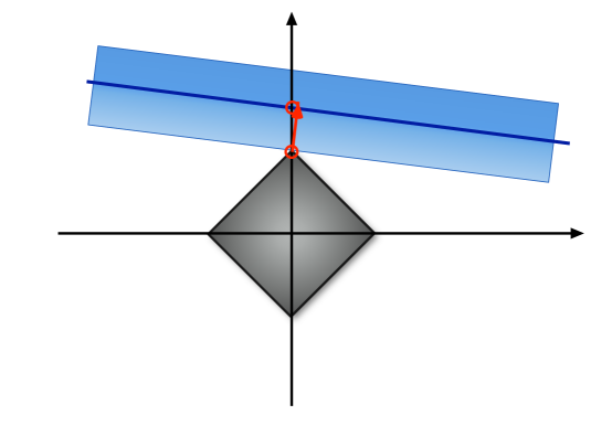
Figure 1: Geometric interpretation for construction of $\bm{\widehat{\theta}}^{u}$. The bias in $\bm{\widehat{\theta}}$ is eliminated by modifying the estimator in the direction of increasing its $\ell_{1}$ norm

3.2 Asymptotic analysis

For given dimension $p$, an instance of the standard Gaussian design model is defined by the tuple $(\bm{\theta}_{0},n,\sigma)$, where $\bm{\theta}_{0}\in{\mathbb{R}}^{p}$, $n\in{\mathbb{N}}$, $\sigma\in{\mathbb{R}}_{+}$. We consider sequences of instances indexed by the problem dimension $\{(\bm{\theta}_{0}(p),n(p),\sigma(p))\}_{p\in{\mathbb{N}}}$.

Definition 3.1.

The sequence of instances $\{(\bm{\theta}_{0}(p),n(p),\sigma(p))\}_{p\in{\mathbb{N}}}$ indexed by $p$ is said to be a converging sequence if $n(p)/p\to\delta\in(0,\infty)$, $\sigma(p)^{2}/n\to\sigma_{0}^{2}$, and the empirical distribution of the entries $\bm{\theta}_{0}(p)$ converges weakly to a probability measure $p_{\Theta_{0}}$ on ${\mathbb{R}}$ with bounded second moment. Further $p^{-1}\sum_{i\in[p]}\theta_{0,i}(p)^{2}\to{\mathbb{E}}_{p_{\Theta_{0}}}\{\Theta_{0}^{2}\}$.

Note that this definition assumes the coefficients $\theta_{0,i}$ are of order one, while the noise is scaled as $\sigma(p)^{2}=\Theta(n)$. Equivalently, we could have assumed $\theta_{0,i}=\Theta(1/\sqrt{n})$ and $\sigma^{2}(p)=\Theta(1)$: the two settings only differ by a scaling of ${\bm{y}}$. We favor the first scaling as it simplifies somewhat the notation in the following.

As before, we will measure the quality of the proposed test in terms of its significance level (size) $\alpha$ and power $1-\beta$. Recall that $\alpha$ and $\beta$ respectively indicate the type I error (false positive) and type II error (false negative) rates. The following theorem establishes that the $P_{i}$’s are indeed valid p-values, i.e., allow to control type I errors. Throughout $S_{0}(p)=\{i\in[p]:\theta_{0,i}(p)\neq 0\}$ is the support of $\bm{\theta}_{0}(p)$.

Theorem 3.2.

Let $\{(\bm{\theta}_{0}(p),n(p),\sigma(p))\}_{p\in{\mathbb{N}}}$ be a converging sequence of instances of the standard Gaussian design model. Assume $\lim_{p\to\infty}|S_{0}(p)|/p={\mathbb{P}}(\Theta_{0}\neq 0)$. Then, for $i\in S_{0}^{c}(p)$, we have

$$\lim_{p\to\infty}{\mathbb{P}}_{\bm{\theta}_{0}(p)}(T_{i,{\bm{X}}}({\bm{y}})=1)=\alpha\,.$$ (19)

A more general form of Theorem 3.2 (cf. Theorem 4.3) is proved in Section 7. We indeed prove the stronger claim that the following holds true almost surely

$$\lim_{p\to\infty}\frac{1}{|S^{c}_{0}(p)|}\sum_{i\in S^{c}_{0}(p)}T_{i,{\bm{X}}}({\bm{y}})=\alpha\,.$$ (20)

The result of Theorem 3.2 follows then by taking the expectation of both sides of Eq. (20) and using bounded convergence theorem and exchangeability of the columns of ${\bm{X}}$.

Our next theorem proves a lower bound for the power of the proposed test. In order to obtain a non-trivial result, we need to make suitable assumption on the parameter vectors $\bm{\theta}_{0}=\bm{\theta}_{0}(p)$. In particular, we need to assume that the non-zero entries of $\bm{\theta}_{0}$ are lower bounded in magnitude. If this were not the case, it would be impossible to distinguish arbitrarily small parameters $\theta_{0,i}$ from $\theta_{0,i}=0$. (In Appendix B, we also provide an explicit formula for the regularization parameter $\lambda=\lambda(p_{\Theta_{0}},\sigma,{\varepsilon},\delta)$ that achieves this power.)

Theorem 3.3.

There exists a (deterministic) choice of $\lambda=\lambda(\sigma,{\varepsilon})$ such that the following happens.

Let $\{(\bm{\theta}_{0}(p),n(p),\sigma(p))\}_{p\in{\mathbb{N}}}$ be a converging sequence of instances under the standard Gaussian design model. Assume that $|S_{0}(p)|\leq{\varepsilon}p$, and for all $i\in S_{0}(p)$, $|\theta_{0,i}(p)|\geq\mu$ with $\mu=\mu_{0}\sigma(p)/\sqrt{n(p)}$. for $i\in S_{0}(p)$, we have

$$\lim_{p\to\infty}{\mathbb{P}}_{\bm{\theta}_{0}(p)}(T_{i,{\bm{X}}}({\bm{y}})=1)\geq G\Big{(}\alpha,\frac{\mu_{0}}{\tau_{*}}\Big{)}\,,$$ (21)

where $\tau_{*}=\tau_{*}(\sigma_{0},{\varepsilon},\delta)$ is defined as follows

$$\tau_{*}^{2} =\begin{cases}\dfrac{1}{1-M({\varepsilon})/\delta},&\text{if }\delta>M({\varepsilon}),\\ \infty,&\text{if }\delta\leq M({\varepsilon}).\end{cases}$$ (22)

Here, $M({\varepsilon})$ is given by the following parametric expression in terms of the parameter $\kappa\in(0,\infty)$:

$${\varepsilon}=\frac{2(\phi(\kappa)-\kappa\Phi(-\kappa))}{\kappa+2(\phi(\kappa)-\kappa\Phi(-\kappa))},\;\;\;\;\;\;\;\;\;M({\varepsilon})=\frac{2\phi(\kappa)}{\kappa+2(\phi(\kappa)-\kappa\Phi(-\kappa))}.$$ (23)

Theorem 3.3 is proved in Section 7. We indeed prove the stronger claim that the following holds true almost surely:

$$\lim_{p\to\infty}\frac{1}{|S_{0}(p)|}\sum_{i\in S_{0}(p)}T_{i,{\bm{X}}}({\bm{y}})\geq G\Big{(}\alpha,\frac{\mu_{0}}{\tau_{*}}\Big{)}\,.$$ (24)

The result of Theorem 3.3 follows then by taking the expectation of both sides of Eq. (24) and using exchangeability of the columns of ${\bm{X}}$.

Again, it is convenient to rephrase Theorem 3.3 in terms of the minimum value of $\mu$ for which we can achieve statistical power $1-\beta\in(\alpha,1)$ at significance level $\alpha$. It is known that $M({\varepsilon})=2{\varepsilon}\log(1/{\varepsilon})\,(1+O({\varepsilon}))$ [11]. Hence, for $n\geq 2\,s_{0}\log(p/s_{0})\,(1+O(s_{0}/p))$, we have $\tau_{*}^{2}=O(1)$. Since $\lim_{u\to\infty}G(\alpha,u)=1$, any pre-assigned statistical power can be achieved by taking $\mu\geq C({\varepsilon},\delta)\sigma/\sqrt{n}$ which matches the fundamental limit established in the previous section.

Let us finally comment on the choice of the regularization parameter $\lambda$. Theorem 3.2 holds irrespective of $\lambda$, as long as it is kept fixed in the asymptotic limit. In other words, control of type I errors is fairly insensitive to the regularization parameters. On the other hand, to achieve optimal minimax power, it is necessary to tune $\lambda$ to the correct value. The tuned value of $\lambda=\lambda(p_{\Theta_{0}},\sigma,{\varepsilon},\delta)$ for the standard Gaussian sequence model is provided in Appendix A. Further, the factor $\sigma$ (and hence the need to estimate the noise level) can be omitted if –instead of the Lasso– we use the scaled Lasso [30]. In subsection 3.4, we discuss another way of choosing $\lambda$ that also avoid estimating the noise level.

3.3 Gaussian limit

Theorems 3.2 and 3.3 are based on an asymptotic distributional characterization of the Lasso estimator developed in [10]. We restate it here for the reader’s convenience.

Theorem 3.4 ([10]).

Let $\{(\bm{\theta}_{0}(p),n(p),\sigma(p))\}_{p\in{\mathbb{N}}}$ be a converging sequence of instances of the standard Gaussian design model. Denote by $\bm{\widehat{\theta}}=\bm{\widehat{\theta}}({\bm{y}},{\bm{X}},\lambda)$ the Lasso estimator given as per Eq. (4) and define $\bm{\widehat{\theta}}^{u}\in{\mathbb{R}}^{p}$, $\bm{r}\in{\mathbb{R}}^{n}$ by letting

$$\bm{\widehat{\theta}}^{u}\equiv\bm{\widehat{\theta}}+\frac{{\sf d}}{n}\,{\bm{X}}^{\sf T}(\bm{y}-{\bm{X}}\bm{\widehat{\theta}})\,,\;\;\;\;\;\;\bm{r}\equiv\frac{{\sf d}}{\sqrt{n}}(\bm{y}-{\bm{X}}\bm{\widehat{\theta}})\,,$$ (25)

with ${\sf d}=(1-\|\bm{\widehat{\theta}}\|_{0}/n)^{-1}$.

Then, with probability one, the empirical distribution of $\{(\theta_{0,i},\widehat{\theta}^{u}_{i})\}_{i=1}^{p}$ converges weakly to the probability distribution of $(\Theta_{0},\Theta_{0}+\tau_{0}Z)$, for some $\tau_{0}\in{\mathbb{R}}$, where $Z\sim{\sf N}(0,1)$, and $\Theta_{0}\sim p_{\Theta_{0}}$ is independent of $Z$. Furthermore, with probability one, the empirical distribution of $\{r_{i}\}_{i=1}^{p}$ converges weakly to ${\sf N}(0,\tau^{2}_{0})$.

Finally $\tau_{0}\in{\mathbb{R}}$ is defined by the unique solution of Eqs. (103) and (104) in Appendix A.

In particular, this result implies that the empirical distribution of $\{\widehat{\theta}^{u}_{i}-\theta_{0,i}\}_{i=1}^{p}$ is asymptotically normal with variance $\tau_{0}^{2}$. This naturally motivates the use of $|\widehat{\theta}^{u}_{i}|/\tau_{0}$ as a test statistics for hypothesis $H_{0,i}:\,\theta_{0,i}=0$.

The definitions of ${\sf d}$ and $\tau$ in step 2 are also motivated by Theorem 3.4. In particular, ${\sf d}(\bm{y}-{\bm{X}}\bm{\widehat{\theta}})/\sqrt{n}$ is asymptotically normal with variance $\tau_{0}^{2}$. This is used in step 2, where $\tau$ is just the robust median absolute deviation (MAD) estimator (we choose this estimator since it is more resilient to outliers than the sample variance [31]).

3.4 Numerical experiments

As an illustration, we generated synthetic data from the linear model (1) with $\bm{w}\sim{\sf N}(0,{\rm I}_{p\times p})$ and the following configurations.

Design matrix: For pairs of values $(n,p)=\{(300,1000),(600,1000),(600,2000)\}$, the design matrix is generated from a realization of $n$ i.i.d. rows $\bm{x}_{i}\sim{\sf N}(0,{\rm I}_{p\times p})$.

Regression parameters: We consider active sets $S_{0}$ with $|S_{0}|=s_{0}\in\{10,20,25,50,100\}$, chosen uniformly at random from the index set $\{1,\cdots,p\}$. We also consider two different strengths of active parameters $\theta_{0,i}=\mu$, for $i\in S_{0}$, with $\mu\in\{0.1,0.15\}$.

We examine the performance of SDL-test  (cf. Table 1) at significance levels $\alpha=0.025,0.05$. The experiments are done using glmnet-package in R that fits the entire Lasso path for linear regression models. Let ${\varepsilon}=s_{0}/p$ and $\delta=n/p$. We do not assume ${\varepsilon}$ is known, but rather estimate it as $\bar{{\varepsilon}}=0.25\,\delta/\log(2/\delta)$. The value of $\bar{{\varepsilon}}$ is half the maximum sparsity level ${\varepsilon}$ for the given $\delta$ such that the Lasso estimator can correctly recover the parameter vector if the measurements were noiseless [32, 10]. Provided it makes sense to use Lasso at all, $\bar{{\varepsilon}}$ is thus a reasonable ballpark estimate.

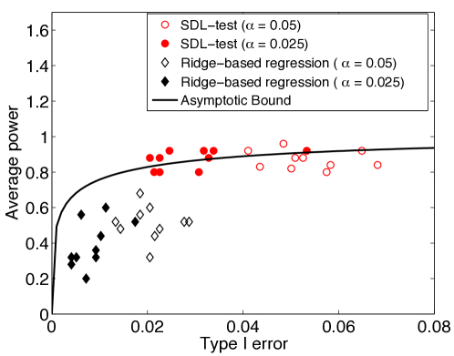
Figure 2: Comparison between SDL-test (Table 1), ridge-based regression [17] and the asymptotic bound for SDL-test  (established in Theorem 3.3). Here, $p=1000,n=600,s_{0}=25,\mu=0.15$.

Method	Type I err	Type I err	Avg. power	Avg. power
	(mean)	(std.)	(mean)	(std)
SDL-test $(1000,600,100,0.1)$	0.05422	0.01069	0.44900	0.06951
Ridge-based regression $(1000,600,100,0.1)$	0.01089	0.00358	0.13600	0.02951
LDPE  $(1000,600,100,0.1)$	0.02012	0.00417	0.29503	0.03248
Asymptotic Bound $(1000,600,100,0.1)$	0.05	NA	0.37692	NA
SDL-test $(1000,600,50,0.1)$	0.04832	0.00681	0.52000	0.06928
Ridge-based regression $(1000,600,50,0.1)$	0.01989	0.00533	0.17400	0.06670
LDPE  $(1000,600,50,0.1)$	0.02211	0.01031	0.20300	0.08630
Asymptotic Bound $(1000,600,50,0.1)$	0.05	NA	0.51177	NA
SDL-test $(1000,600,25,0.1)$	0.05662	0.01502	0.56400	0.11384
Ridge-based regression $(1000,600,25,0.1)$	0.02431	0.00536	0.25600	0.06586
LDPE  $(1000,600,25,0.1)$	0.02305	0.00862	0.27900	0.07230
Asymptotic Bound $(1000,600,25,0.1)$	0.05	NA	0.58822	NA

Table 2: Comparison between SDL-test (Table 1), ridge-based regression [17], LDPE [16] and the asymptotic bound for SDL-test  (established in Theorem 3.3) on the setup described in Section 3.4. The significance level is $\alpha=0.05$. The means and the standard deviations are obtained by testing over $10$ realizations of the corresponding configuration. Here a quadruple such as $(1000,600,50,0.1)$ denotes the values of $p=1000$, $n=600$, $s_{0}=50$, $\mu=0.1$.

The regularization parameter $\lambda$ is chosen as to satisfy

$$\lambda{\sf d}=\kappa_{*}\tau$$ (26)

where $\tau$ and ${\sf d}$ are determined in step 2 of the procedure. Here $\kappa_{*}=\kappa_{*}(\bar{{\varepsilon}})$ is the minimax threshold value for estimation using soft thresholding in the Gaussian sequence model, see [11] and Remark B.1. Note that $\tau$ and ${\sf d}$ in the equation above depend implicitly upon $\lambda$. Since glmnet returns the entire Lasso path, the value of $\lambda$ solving the above equation can be computed by the bisection method.

As mentioned above, the control of type I error is fairly robust for a wide range of values of $\lambda$. However, the above is an educated guess based on the analysis of [32, 10]. We also tried the values of $\lambda$ proposed for instance in [26, 17] on the basis of oracle inequalities.

Figure 2 shows the results of SDL-test and the method of [17] for parameter values $p=1000,n=600,s_{0}=25,\mu=0.15$, and significance levels $\alpha\in\{0.025,0.05\}$. Each point in the plot corresponds to one realization of this configuration (there are a total of $10$ realizations). We also depict the theoretical curve $(\alpha,G(\alpha,\mu_{0}/\tau_{*}))$, predicted by Theorem 3.3. The empirical results are in good agreement with the asymptotic prediction.

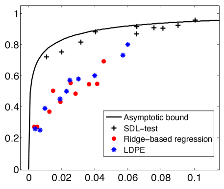
Figure 3: Comparison between SDL-test , ridge-based regression [17], and LDPE [16]. The curve corresponds to the asymptotic bound for SDL-test  as established in Theorem 3.3. For the same values of type I error achieved by methods, SDL-test  results in a higher statistical power. Here, $p=1000,n=600,s_{0}=25,\mu=0.15$.

We compare SDL-test  with the ridge-based regression method [17] and the low dimensional projection estimator (LDPE )  [16]. Table 2 summarizes the results for a few configurations $(p,n,s_{0},\mu)$, and $\alpha=0.05$. Simulation results for a larger number of configurations and $\alpha=0.05,0.025$ are reported in Tables 8 and 9 in Appendix E.

As demonstrated by these results, LDPE [16] and the ridge-based regression [17] are both overly conservative. Namely, they achieve smaller type I error than the prescribed level $\alpha$ and this comes at the cost of a smaller statistical power than our testing procedure. This is to be expected since the approach of [17] and [16] cover a broader class of design matrices ${\bm{X}}$, and are not tailored to random designs.

Note that being overly conservative is a drawback, when this comes at the expense of statistical power. The data analysts should be able to decide the level of statistical significance $\alpha$, and obtain optimal statistical power at that level.

The reader might wonder whether the loss in statistical power of methods in [17] and [16] is entirely due to the fact that these methods achieve a smaller number of false positives than requested. In Fig. 3, we run SDL-test , ridge-based regression [17], and LDPE  for $\alpha\in\{0.01,0.02,\cdots,0.1\}$ and for $10$ realizations of the problem per each value of $\alpha$. We plot the average type I error and the average power of each method versus $\alpha$. As we see even for the same empirical fraction of type I errors, SDL-test  results in a higher statistical power.

4 Hypothesis testing for nonstandard Gaussian designs

In this section, we generalize our testing procedure to nonstandard Gaussian design models where the rows of the design matrix ${\bm{X}}$ are drawn independently from distribution ${\sf N}(0,\bm{\Sigma})$.

We first describe the generalized SDL-test  procedure in subsection 4.1 under the assumption that $\bm{\Sigma}$ is known. In subsection 4.2, we show that this generalization can be justified from a certain generalization of the Gaussian limit theorem 3.4 to nonstandard Gaussian designs.

Establishing such a generalization of Theorem 3.4 appears extremely challenging. We nevertheless show that such a limit theorem follows from the replica method of statistical physics in section 4.4. We also show that a version of this limit theorem is relatively straightforward in the regime $s_{0}=o(n/(\log p)^{2})$.

Finally, in Section 4.5 we discuss a procedure for estimating the covariance $\bm{\Sigma}$ (cf. Subroutine  in Table 4). Appendix F proposes an alternative implementation that does not estimate $\bm{\Sigma}$ but instead bounds the effect of unknown $\bm{\Sigma}$.

4.1 Hypothesis testing procedure

Table 3: SDL-test  for testing hypothesis $H_{0,i}$ under nonstandard Gaussian design model

 
SDL-test: Testing hypothesis $H_{0,i}$ under nonstandard Gaussian design model.
 
Input: regularization parameter $\lambda$, significance level $\alpha$, covariance matrix $\bm{\Sigma}$
Output: p-values $P_{i}$, test statistics $T_{i,{\bm{X}}}({\bm{y}})$
1: Let

$$\bm{\widehat{\theta}}(\lambda)=\text{argmin}_{\bm{\theta}\in{\mathbb{R}}^{p}}\,\,\Big{\{}\frac{1}{2n}\|{\bm{y}}-{\bm{X}}\bm{\theta}\|^{2}+\lambda\|\bm{\theta}\|_{1}\Big{\}}.$$

2: Let

$${\sf d}=\left(1-\frac{1}{n}\|\bm{\widehat{\theta}}(\lambda)\|_{0}\right)^{-1},\;\;\;\;\;\tau=\frac{1}{\Phi^{-1}(0.75)}\frac{{\sf d}}{\sqrt{n}}|(\bm{y}-{\bm{X}}\bm{\widehat{\theta}}(\lambda))|_{(n/2)},$$ (27)

where for $\bm{v}\in{\mathbb{R}}^{K}$, $|\bm{v}|_{\ell}$ is the $\ell$-th largest entry in the vector $(|v_{1}|,\cdots,|v_{n}|)$.
3: Let

$$\bm{\widehat{\theta}}^{u}=\bm{\widehat{\theta}}(\lambda)+\frac{{\sf d}}{n}\bm{\Sigma}^{-1}{\bm{X}}^{\sf T}(\bm{y}-{\bm{X}}\bm{\widehat{\theta}}(\lambda)).$$

4: Assign the p-values $P_{i}$ for the test $H_{0,i}$ as follows.

$$P_{i}=2\bigg{(}1-\Phi\Big{(}\Big{|}\frac{\widehat{\theta}^{u}_{i}}{\tau[(\bm{\Sigma}^{-1})_{ii}]^{1/2}}\Big{|}\Big{)}\bigg{)}.$$

5: The decision rule is then based on the p-values:

$$T_{i,{\bm{X}}}({\bm{y}})=\begin{cases}1&\text{if $P_{i}\leq\alpha$}\quad\quad\;(\text{reject the null hypothesis }H_{0,i}),\\ 0&\text{otherwise}\quad\quad\text{(accept the null hypothesis)}.\end{cases}$$

 

The hypothesis testing procedure SDL-testfor general Gaussian designs is defined in Table 3.

The basic intuition of this generalization is that $(\widehat{\theta}^{u}_{i}-\widehat{\theta}_{0,i})/(\tau[(\bm{\Sigma}^{-1})_{ii}]^{1/2})$ is expected to be asymptotically ${\sf N}(0,1)$, whence the definition of (two-sided) p-values $P_{i}$ follows as in step 4. Parameters ${\sf d}$ and $\tau$ in step 2 are defined in the same manner to the standard Gaussian designs.

4.2 Asymptotic analysis

For given dimension $p$, an instance of the nonstandard Gaussian design model is defined by the tuple $(\bm{\Sigma},\bm{\theta}_{0},n,\sigma)$, where $\bm{\Sigma}\in{\mathbb{R}}^{p\times p}$, $\bm{\Sigma}\succ 0$, $\bm{\theta}_{0}\in{\mathbb{R}}^{p}$, $n\in{\mathbb{N}}$, $\sigma\in{\mathbb{R}}_{+}$. We are interested in the asymptotic properties of sequences of instances indexed by the problem dimension $\{(\bm{\Sigma}(p),\bm{\theta}_{0}(p),n(p),\sigma(p))\}_{p\in{\mathbb{N}}}$. Motivated by Proposition 3.4, we define a property of a sequence of instances that we refer to as standard distributional limit.

Definition 4.1.

A sequence of instances $\{(\bm{\Sigma}(p),\bm{\theta}_{0}(p),n(p),\sigma(p))\}_{p\in{\mathbb{N}}}$ indexed by $p$ is said to have an (almost sure) standard distributional limit if there exist $\tau,{\sf d}\in{\mathbb{R}}$ (with ${\sf d}$ potentially random, and both $\tau$, ${\sf d}$ potentially depending on $p$), such that the following holds. Denote by $\bm{\widehat{\theta}}=\bm{\widehat{\theta}}(y,{\bm{X}},\lambda)$ the Lasso estimator given as per Eq. (4) and define $\bm{\widehat{\theta}}^{u}\in{\mathbb{R}}^{p}$, $\bm{r}\in{\mathbb{R}}^{n}$ by letting

$$\bm{\widehat{\theta}}^{u}\equiv\bm{\widehat{\theta}}+\frac{{\sf d}}{n}\,\bm{\Sigma}^{-1}{\bm{X}}^{\sf T}(\bm{y}-{\bm{X}}\bm{\widehat{\theta}})\,,\;\;\;\;\;\bm{r}\equiv\frac{{\sf d}}{\sqrt{n}}(\bm{y}-{\bm{X}}\bm{\widehat{\theta}}).$$ (28)

Let $v_{i}=(\theta_{0,i},(\widehat{\theta}^{u}_{i}-\theta_{0,i})/\tau,(\bm{\Sigma}^{-1})_{ii})$, for $1\leq i\leq p$, and $\nu^{(p)}$ be the empirical distribution of $\{v_{i}\}_{i=1}^{p}$ defined as

$$\nu^{(p)}=\frac{1}{p}\sum_{i=1}^{p}\delta_{v_{i}}\,,$$ (29)

where $\delta_{v_{i}}$ denotes the Dirac delta function centered at $v_{i}$. Then, with probability one, the empirical distribution $\nu^{(p)}$ converges weakly to a probability measure $\nu$ on ${\mathbb{R}}^{3}$ as $p\to\infty$. Here, $\nu$ is the probability distribution of $(\Theta_{0},\Upsilon^{1/2}Z,\Upsilon)$, where $Z\sim{\sf N}(0,1)$, and $\Theta_{0}$ and $\Upsilon$ are random variables independent of $Z$. Furthermore, with probability one, the empirical distribution of $\{r_{i}/\tau\}_{i=1}^{n}$ converges weakly to ${\sf N}(0,1)$.

Remark 4.2.

This definition is non-empty by Theorem 3.4. Indeed, if $\{(\bm{\theta}_{0}(p),n(p),\sigma(p))\}_{p\in{\mathbb{N}}}$ is converging as per Definition 3.1, and $a>0$ is a constant, then Theorem 3.4 states that $\{(\bm{\Sigma}(p)=a\,{\rm I}_{p\times p},\bm{\theta}_{0}(p),n(p),\sigma(p))\}_{p\in{\mathbb{N}}}$ has a standard distributional limit.

Proving the standard distributional limit for general sequences $\{(\bm{\Sigma}(p),\bm{\theta}_{0}(p),$ $n(p),\sigma(p))\}_{p\in{\mathbb{N}}}$ is an outstanding mathematical challenge. In sections 4.4 and 5 we discuss both rigorous and non-rigorous evidence towards its validity. The numerical simulations in Sections 4.6 and 5 further support the usefulness of this notion.

We will next show that the SDL-test  procedure is appropriate for any random design model for which the standard distributional limit holds. Our first theorem is a generalization of Theorem 3.2 to this setting.

Theorem 4.3.

Let $\{(\bm{\Sigma}(p),\bm{\theta}_{0}(p),n(p),\sigma(p))\}_{p\in{\mathbb{N}}}$ be a sequence of instances for which a standard distributional limit holds. Further assume $\lim_{p\to\infty}|S_{0}(p)|/p={\mathbb{P}}(\Theta_{0}\neq 0)$. Then,

$$\lim_{p\to\infty}\frac{1}{|S^{c}_{0}(p)|}\sum_{i\in S^{c}_{0}(p)}{\mathbb{P}}_{\bm{\theta}_{0}(p)}(T_{i,{\bm{X}}}({\bm{y}})=1)=\alpha\,.$$ (30)

The proof of Theorem 4.3 is deferred to Section 7. In the proof, we show the stronger result that the following holds true almost surely

$$\lim_{p\to\infty}\frac{1}{|S^{c}_{0}(p)|}\sum_{i\in S^{c}_{0}(p)}T_{i,{\bm{X}}}({\bm{y}})=\alpha\,.$$ (31)

The result of Theorem 4.3 follows then by taking the expectation of both sides of Eq. (31) and using bounded convergence theorem.

The following theorem characterizes the power of SDL-test  for general $\bm{\Sigma}$, and under the assumption that a standard distributional limit holds .

Theorem 4.4.

Let $\{(\bm{\Sigma}(p),\bm{\theta}_{0}(p),n(p),\sigma(p))\}_{p\in{\mathbb{N}}}$ be a sequence of instances with standard distributional limit. Assume (without loss of generality) $\sigma(p)=\sqrt{n(p)}$, and further $|\theta_{0,i}(p)|/[(\bm{\Sigma}^{-1})_{ii}]^{1/2}\geq\mu_{0}$ for all $i\in S_{0}(p)$, and $\lim_{o\to\infty}|S_{0}(p)|/p={\mathbb{P}}(\Theta_{0}\neq 0)\in(0,1)$. Then,

$$\lim_{p\to\infty}\frac{1}{|S_{0}(p)|}\sum_{i\in S_{0}(p)}{\mathbb{P}}_{\bm{\theta}_{0}(p)}(T_{i,{\bm{X}}}({\bm{y}})=1)\geq G\Big{(}\alpha,\frac{\mu_{0}}{\tau}\Big{)}\,.$$ (32)

Theorem 4.4 is proved in Section 7. We indeed prove the stronger result that the following holds true almost surely

$$\lim_{p\to\infty}\frac{1}{|S_{0}(p)|}\sum_{i\in S_{0}(p)}T_{i,{\bm{X}}}({\bm{y}})\geq G\Big{(}\alpha,\frac{\mu_{0}}{\tau}\Big{)}\,.$$ (33)

We also notice that in contrast to Theorem 3.3, where $\tau_{*}$ has an explicit formula that leads to an analytical lower bound for the power (for a suitable choice of $\lambda$), in Theorem 4.4, $\tau$ depends upon $\lambda$ implicitly and can be estimated from the data as in step 3 of SDL-test  procedure. The result of Theorem 4.4 holds for any value of $\lambda$.

4.3 Gaussian limit for $n\gg s_{0}(\log p)^{2}$

In the following theorem we show that if sample size $n$ asymptotically dominates $s_{0}(\log p)^{2}$, then the standard distributional limit can be established rigorously.

Theorem 4.5.

Assume the sequence of instances $\{\bm{\Sigma}(p),\bm{\theta}_{0}(p),n(p),\sigma(p)\}_{p\in{\mathbb{N}}}$ such that, as $p\to\infty$ (letting $s_{0}=\|\bm{\theta}_{0}(p)\|_{0}$):

• $n(p)\leq p$, and $s_{0}(\log p)^{2}/n(p)\to 0$;

• $\sigma(p)^{2}/n(p)\to\sigma_{0}^{2}>0$;

• There exist constants $c_{\rm min},c_{\rm max}>0$ such that the eigenvalues of $\bm{\Sigma}$ lie in the interval $[c_{\rm min},c_{\rm max}]$: $c_{\rm min}\leq\lambda_{\rm min}(\bm{\Sigma})\leq\lambda_{\rm max}(\bm{\Sigma})\leq c_{\rm max}$;

• The empirical distribution of $\{(\bm{\Sigma}^{-1})_{ii})\}_{1\leq i\leq p}$ converges weakly to the probability distribution of the random variable $\Upsilon$;

• The regularization parameter is $\lambda=C_{*}\sigma\sqrt{(\log p)/n}$ for $C_{*}=C_{*}(c_{\rm min},c_{\rm max})$ a sufficiently large constant.

Then the sequence has a standard distributional limit with ${\sf d}=(1-\|\bm{\widehat{\theta}}(\lambda)\|_{0}/n)^{-1}$ and $\tau=\sigma_{0}$. Alternatively, $\tau$ can be taken to be a solution of Eq. (37) below.

Theorem 4.5 is proved in Section 7.7. The proof uses techniques from our conference paper [33].

Notice that this result does allow to control type I errors using Theorem 4.3, but does not allow to lower bound the power, using Theorem 4.4, since $|S_{0}(p)|/p\to 0$. A lower bound on the power under the same assumptions presented in this section can be found in [33]. In the present paper we focus instead on the case $|S_{0}(p)|/p$ bounded away from $0$.

4.4 Gaussian limit via the replica heuristics for smaller sample size $n$

As mentioned above, the standard distributional limit follows from Theorem 3.4 for $\Sigma={\rm I}_{p\times p}$. Even in this simple case, the proof is rather challenging [10]. Partial generalization to non-gaussian designs and other convex problems appeared recently in [34] and [35], each requiring over 50 pages of proofs.

On the other hand, these and similar asymptotic results can be derived heuristically using the ‘replica method’ from statistical physics. In Appendix D, we use this approach to derive the following claim.

Replica Method Claim 4.6.

Assume the sequence of instances $\{(\bm{\Sigma}(p),\bm{\theta}_{0}(p),n(p),\sigma(p))\}_{p\in{\mathbb{N}}}$ to be such that, as $p\to\infty$: $(i)$ $n(p)/p\to\delta>0$; $(ii)$ $\sigma(p)^{2}/n(p)\to\sigma_{0}^{2}>0$; $(iii)$ The sequence of functions

$${\mathfrak{E}}^{(p)}(a,b)\equiv\frac{1}{p}\,{\mathbb{E}}\min_{\bm{\theta}\in{\mathbb{R}}^{p}}\Big{\{}\frac{b}{2}\|\bm{\theta}-\bm{\theta}_{0}-\sqrt{a}\bm{\Sigma}^{-1/2}\bm{z}\|_{\bm{\Sigma}}^{2}+\lambda\|\bm{\theta}\|_{1}\Big{\}}\,,$$ (34)

with $\|\bm{v}\|_{\bm{\Sigma}}^{2}\equiv\langle\bm{v},\bm{\Sigma}\bm{v}\rangle$ and $\bm{z}\sim{\sf N}(0,{\rm I}_{p\times p})$ admits a differentiable limit ${\mathfrak{E}}(a,b)$ on ${\mathbb{R}}_{+}\times{\mathbb{R}}_{+}$, with $\nabla{\mathfrak{E}}^{(p)}(a,b)\to\nabla{\mathfrak{E}}(a,b)$. Then the sequence has a standard distributional limit. Further let

$$\eta_{b}({\bm{y}}) \equiv\underset{\bm{\theta}\in{\mathbb{R}}^{p}}{\arg\min}\Big{\{}\frac{b}{2}\|\bm{\theta}-{\bm{y}}\|_{\bm{\Sigma}}^{2}+\lambda\|\bm{\theta}\|_{1}\Big{\}}\,,$$ (35)

$${\sf E}_{1}(a,b) \equiv\lim_{p\to\infty}\frac{1}{p}{\mathbb{E}}\big{\{}\big{\|}\eta_{b}(\bm{\theta}_{0}+\sqrt{a}\bm{\Sigma}^{-1/2}\bm{z})-\bm{\theta}_{0}\big{\|}_{\bm{\Sigma}}^{2}\big{\}}\,,$$ (36)

where the the limit exists by the above assumptions on the convergence of ${\mathfrak{E}}^{(p)}(a,b)$. Then, the parameters $\tau$ and ${\sf d}$ of the standard distributional limit are obtained by setting ${\sf d}=(1-\bm{\widehat{\theta}}/n)^{-1}$ and solving the following with respect to $\tau^{2}$:

$$\tau^{2}=\sigma_{0}^{2}+\frac{1}{\delta}\,{\sf E}_{1}(\tau^{2},1/{\sf d})\,.$$ (37)

In other words, the replica method indicates that the standard distributional limit holds for a large class of non-diagonal covariance structures $\bm{\Sigma}$. It is worth stressing that convergence assumption for the sequence ${\mathfrak{E}}^{(p)}(a,b)$ is quite mild, and is satisfied by a large family of covariance matrices. For instance, it can be proved that it holds for block-diagonal matrices $\bm{\Sigma}$ as long as the blocks have bounded length and the blocks empirical distribution converges.

The replica method is a non-rigorous but highly sophisticated calculation procedure that has proved successful in a number of very difficult problems in probability theory and probabilistic combinatorics. Attempts to make the replica method rigorous have been pursued over the last 30 years by some world-leading mathematicians [36, 37, 38, 39]. This effort achieved spectacular successes, but so far does not provide tools to prove the above replica claim. In particular, the rigorous work mainly focuses on ‘i.i.d. randomness’, corresponding to the case covered by Theorem 3.4.

Over the last ten years, the replica method has been used to derive a number of fascinating results in information theory and communications theory, see e.g. [40, 41, 42, 43, 44]. More recently, several groups used it successfully in the analysis of high-dimensional sparse regression under standard Gaussian designs [45, 46, 47, 44, 48, 49, 50]. The rigorous analysis of ours and other groups [51, 10, 34, 35] subsequently confirmed these heuristic calculations in several cases.

There is a fundamental reason that makes establishing the standard distributional limit a challenging task. This requires in fact to characterize the distribution of the estimator (4) in a regime where the standard deviation of $\widehat{\theta}_{i}$ is of the same order as its mean. Further, $\widehat{\theta}_{i}$ does not converge to the true value $\theta_{0,i}$, hence making perturbative arguments ineffective.

The analysis becomes easier for a larger number of samples. In Theorem 4.5 below we will show that (a suitable version of) the standard distributional holds for $n$ asymptotically larger than $s_{0}(\log p)^{2}$. This uses methods from our companion paper [20].

4.5 Covariance estimation

So far we assumed that the design covariance $\bm{\Sigma}$ is known. This setting is relevant for semi-supervised learning applications, where the data analyst has access to a large number $N\gg p$ of ‘unlabeled examples’. These are i.i.d. feature vectors $\bm{u}_{1}$, $\bm{u}_{2}$,…$\bm{u}_{N}$ with $\bm{u}_{1}\sim{\sf N}(0,\bm{\Sigma})$ distributed as $\bm{x}_{1}$, for which the response variable $y_{i}$ is not available. In this case $\bm{\Sigma}$ can be estimated accurately by $N^{-1}\sum_{i=1}^{n}\bm{u}_{i}\bm{u}_{i}^{{\sf T}}$. We refer to [52] for further background on such applications.

In other applications, $\bm{\Sigma}$ is unknown and no additional data is available. In this case we proceed as follows:

1. We estimate $\Sigma$ from the design matrix $\bm{X}$ (equivalently, from the feature vectors $\bm{x}_{1}$, $\bm{x}_{2}$, …$\bm{x}_{n}$). We let $\bm{\widehat{\Sigma}}$ denote the resulting estimate.

2. We use $\bm{\widehat{\Sigma}}$ instead of $\bm{\Sigma}$ in step 3 of our hypothesis testing procedure.

The problem of estimating covariance matrices in high-dimensional setting has attracted considerable attention in the past. Several estimation methods provide a consistent estimate $\bm{\widehat{\Sigma}}$, under suitable structural assumptions on $\bm{\Sigma}$. For instance if $\bm{\Sigma}^{-1}$ is sparse, one can apply the graphical model method of [1], the regression approach of [53], or CLIME estimator [54], to name a few.

Since the covariance estimation problem is not the focus of our paper, we will test the above approach using a very simple covariance estimation method. Namely, we assume that $\bm{\Sigma}$ is sparse and estimate it by thresholding the empirical covariance. A detailed description of this estimator is given in Table 4. We refer to [55] for a theoretical analysis of this type of methods. Note that the Lasso is unlikely to perform well if the columns of ${\bm{X}}$ are highly correlated and hence the assumption of sparse $\bm{\Sigma}$ is very natural. On the other hand, we would like to emphasize that this covariance thresholding estimation is only one among many possible approaches.

As an additional contribution, in Appendix F we describe an alternative covariance-free procedure that only uses bounds on $\bm{\Sigma}$ where the bounds are estimated from the data.

In our numerical experiments, we use the estimated covariance returned by Subroutine. As shown in the next section, computed p-values appear to be fairly robust with respect to errors in the estimation of $\bm{\Sigma}$. It would be interesting to develop a rigorous analysis of SDL-test  that accounts for the covariance estimation error.

Table 4: Subroutine  for estimating covariance $\bm{\Sigma}$

 
Subroutine: Estimating covariance matrix $\bm{\Sigma}$
 
Input: Design matrix ${\bm{X}}$
Output: Estimate $\bm{\widehat{\Sigma}}$
1: Let $\bm{C}=(1/n){\bm{X}}^{\sf T}{\bm{X}}\in{\mathbb{R}}^{p\times p}$.
2: Let $\sigma_{1}$ be the empirical variance of the entries in $S$ and let $\mathcal{A}=\{C_{ij}:|C_{ij}|\leq 3\sigma_{1}\}$.
3: Let $\sigma_{2}$ be the variance of entries in $\mathcal{A}$.
4: Construct $\bm{\widehat{C}}$ as follows:

$$\widehat{C}_{ij}=C_{ij}\,{\mathbb{I}}(|C_{ij}|\geq 3\sigma_{2}).$$ (38)

5: Denote by $\zeta_{1}$ and $\zeta_{2}$ the smallest and the smallest positive eigenvalues of $\bm{\widehat{C}}$ respectively.
6: Set

$$\bm{\widehat{\Sigma}}=\bm{\widehat{C}}+(\zeta_{2}-\zeta_{1}){\rm I}\,.$$ (39)

 

4.6 Numerical experiments

In carrying out our numerical experiments for correlated Gaussian designs, we consider the same setup as the one in Section 3.4. The only difference is that the rows of the design matrix are independently $\bm{x}_{i}\sim{\sf N}(0,\bm{\Sigma})$. We choose $\bm{\Sigma}\in{\mathbb{R}}^{p\times p}$ to be a the symmetric matrix with entries $\Sigma_{jk}$ are defined as follows for $j\leq k$

$$\Sigma_{jk}=\begin{cases}1&\text{if }k=j\,,\\ 0.1&\text{if }k\in\{j+1,\cdots,j+5\}\\ &\text{or }k\in\{j+p-5,\dots,j+p-1\},\\ 0&\text{for all other $j\leq k$.}\end{cases}$$ (40)

Elements below the diagonal are given by the symmetry condition $\Sigma_{kj}=\Sigma_{jk}$. (Notice that this is a circulant matrix.)

In Fig. 4(a), we compare SDL-test with the ridge-based regression method proposed in [17]. While the type I errors of SDL-test  are in good match with the chosen significance level $\alpha$, the method of [17] is conservative. As in the case of standard Gaussian designs, this results in significantly smaller type I errors than $\alpha$ and smaller average power in return. Also, in Fig. 5, we run SDL-test , ridge-based regression [17], and LDPE  [16] for $\alpha\in\{0.01,0.02,\cdots,0.1\}$ and for $10$ realizations of the problem per each value of $\alpha$. We plot the average type I error and the average power of each method versus $\alpha$. As we see, similar to the case of standard Gaussian designs, even for the same empirical fraction of type I errors, SDL-test  results in a higher statistical power.

Table 5 summarizes the performances of the these methods for a few configurations $(p,n,s_{0},\mu)$, and $\alpha=0.05$. Simulation results for a larger number of configurations and $\alpha=0.05,0.025$ are reported in Tables 10 and 11 in Appendix E.

Let $\bm{z}=(z_{i})_{i=1}^{p}$ denote the vector with entries $z_{i}\equiv\widehat{\theta}^{u}_{i}/(\tau[(\bm{\Sigma}^{-1})_{ii}]^{1/2})$. In Fig. 4(b) we plot the normalized histograms of $\bm{z}_{S_{0}}$ (in red) and $\bm{z}_{S_{0}^{c}}$ (in white), where $\bm{z}_{S_{0}}$ and $\bm{z}_{S_{0}^{c}}$ respectively denote the restrictions of $\bm{z}$ to the active set $S_{0}$ and the inactive set $S_{0}^{c}$. The plot clearly exhibits the fact that $\bm{z}_{S^{c}_{0}}$ has (asymptotically) standard normal distribution and the histogram of $\bm{z}_{S_{0}}$ appears as a distinguishable bump. This is the core intuition in defining SDL-test.

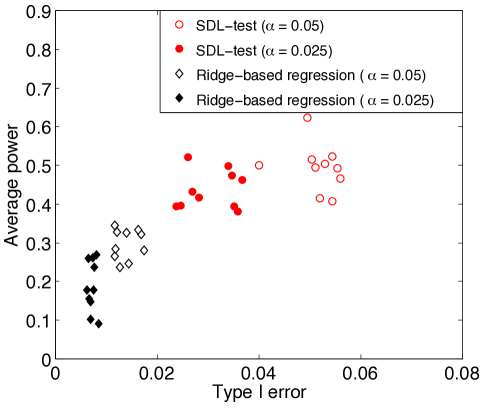
(a) Comparison between SDL-test  and ridge-based regression [17].

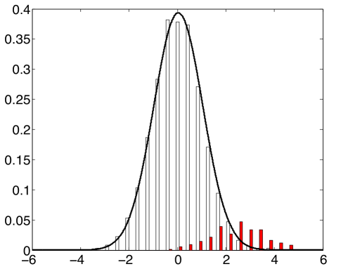
(b) Normalized histograms of $\bm{z}_{S_{0}}$ (in red) and $\bm{z}_{S_{0}^{c}}$ (in white) for one realization.

Figure 4: Numerical results for setting of Section 4.6 and $p=2000$, $n=600$, $s_{0}=50$, $\mu=0.1$.

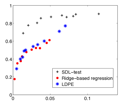
Figure 5: Comparison between SDL-test , ridge-based regression [17], and LDPE [16] in the setting of nonstandard Gaussian designs. For the same values of type I error achieved by methods, SDL-test  results in a higher statistical power. Here, $p=1000,n=600,s_{0}=25,\mu=0.15$.

Method	Type I err	Type I err	Avg. power	Avg. power
	(mean)	(std.)	(mean)	(std)
SDL-test  $(1000,600,100,0.1)$	0.06733	0.01720	0.48300	0.03433
Ridge-based regression $(1000,600,100,0.1)$	0.00856	0.00416	0.17000	0.03828
LDPE  $(1000,600,100,0.1)$	0.01011	0.00219	0.29503	0.03248
Lower bound $(1000,600,100,0.1)$	0.05	NA	0.45685	0.04540
SDL-test  $(1000,600,50,0.1)$	0.04968	0.00997	0.50800	0.05827
Ridge-based regression $(1000,600,50,0.1)$	0.01642	0.00439	0.21000	0.04738
LDPE  $(1000,600,50,0.1)$	0.02037	0.00751	0.32117	0.06481
Lower bound $(1000,600,50,0.1)$	0.05	NA	0.50793	0.03545
SDL-test  $(1000,600,25,0.1)$	0.05979	0.01435	0.55200	0.08390
Ridge-based regression $(1000,600,25,0.1)$	0.02421	0.00804	0.22400	0.10013
LDPE  $(1000,600,25,0.1)$	0.02604	0.00540	0.31008	0.06903
Lower bound $(1000,600,25,0.1)$	0.05	NA	0.54936	0.06176

Table 5: Comparison between SDL-test, ridge-based regression [17], LDPE [16] and the lower bound for SDL-test  power (cf. Theorem 4.4) on the setup described in Section 4.6. The significance level is $\alpha=0.05$. The means and the standard deviations are obtained by testing over $10$ realizations of the corresponding configuration. Here a quadruple such as $(1000,600,50,0.1)$ denotes the values of $p=1000$, $n=600$, $s_{0}=50$, $\mu=0.1$.

5 Discussion

In this section we compare our contribution with related work in order to put it in proper perspective. We first compare it with other recent debiasing methods [16, 19, 20] in subsection 5.1. In subsection 5.2 we then discuss the role of of the factor ${\sf d}$ in our definition of $\bm{\widehat{\theta}}^{u}$: this is an important difference with respect to the methods of [16, 19, 20]. We finally contrast the Gaussian limit in Theorem 3.4 and Le Cam’s local asymptotic normality theory, that plays a pivotal role in classical statistics.

5.1 Comparison with other debiasing methods

As explained several times in the previous sections, the key step in our procedure is to correct the Lasso estimator through a debiasing procedure. For the reader’s convenience, we copy here the definition of the latter:

$$\bm{\widehat{\theta}}^{u}=\bm{\widehat{\theta}}(\lambda)+\frac{{\sf d}}{n}\bm{\Sigma}^{-1}{\bm{X}}^{\sf T}(\bm{y}-{\bm{X}}\bm{\widehat{\theta}}(\lambda)).$$ (41)

The approach of [16] is similar in that it is based on debiased estimator of the form

$$\bm{\widehat{\theta}^{*}}=\bm{\widehat{\theta}}+\frac{1}{n}\bm{M}{\bm{X}}^{\sf T}(\bm{y}-{\bm{X}}\bm{\widehat{\theta}})\,,$$ (42)

where $\bm{M}$ is computed from the design matrix ${\bm{X}}$. The authors of [16] propose to compute $\bm{M}$ by doing sparse regression of each column of ${\bm{X}}$ onto the others.

After a first version of the present paper became available as an online preprint, de Geer, Bühlmann and Ritov [19] studied an approach similar to [16] (and to ours) in a random design setting. They provide guarantees under the assumptions that $\bm{\Sigma}^{-1}$ is sparse and that the sample size $n$ asymptotically dominates $(s_{0}\log p)^{2}$. The authors also establish asymptotic optimality of their method in terms of semiparametric efficiency. The semiparametric setting is also at the center of [16, 29].

A further development over the approaches of [16, 19] was proposed by the present authors in [20]. This paper constructs the matrix $\bm{M}$ by solving an optimization problem that controls the bias of $\bm{\widehat{\theta}^{*}}$ and minimize its variance meanwhile. This method does not require any sparsity assumption on $\bm{\Sigma}$ or $\bm{\Sigma}^{-1}$, but still requires sample size $n$ to asymptotically dominate $(s_{0}\log p)^{2}$.

It is interesting to compare and contrast the results of [16, 19, 20], with the contribution of the present paper. (Let us emphasize that [19] appeared after submission of the present work.)

Assumptions on the design matrix.

The approach of [16, 19, 20] guarantees control of type I error, and optimality for non-Gaussian designs. (Both of [16, 19] require however sparsity of $\bm{\Sigma}^{-1}$.)

In contrast, our results are fully rigorous only in the special case $\bm{\Sigma}={\rm I}$.

Covariance estimation.

Neither of the papers [16, 19, 20] requires knowledge of covariance $\bm{\Sigma}$. The method in [19] estimates $\bm{\Sigma}^{-1}$ assuming that it is sparse, however the method [20] does not require such estimation.

In contrast, our generalization to arbitrary Gaussian designs postulates knowledge of $\bm{\Sigma}$. (Further this generalization relies on the standard distributional limit assumption.)

Sample size assumption.

The work of [19, 20] focuses on random designs, but requires $n$ much larger than $(s_{0}\log p)^{2}$. This is roughly the square of the number of samples needed for consistent estimation.

In contrast, we achieve similar power, and confidence intervals with optimal sample size $n=O(s_{0}\log(p/s_{0}))$.

In summary, the present work is complementary to the one in [16, 19, 20] in that it provides a sharper characterization, within a more restrictive setting. Together, these papers provide support for the use of debiasing methods of the form (42).

5.2 Role of the factor ${\sf d}$

It is worth stressing one subtle, yet interesting, difference between the methods of of [16, 19] and the one of the present paper. In both cases, a debiased estimator is constructed using Eq. (42). However:

• The approach of [16, 19] sets $\bm{M}$ to be an estimate of $(\bm{\Sigma}^{-1})$. In the idealized situation where $\bm{\Sigma}$ is known, this construction reduces to setting $\bm{M}=\bm{\Sigma}^{-1}$.

• In contrast, our prescription (41) amounts to setting $\bm{M}={\sf d}\,\bm{\Sigma}^{-1}$, with ${\sf d}=(1-\|\bm{\widehat{\theta}}\|_{0}/n)^{-1}$. In other words, we choose $\bm{M}$ as a scaled version of the inverse covariance.

The mathematical reason for the specific scaling factor is elucidated by the proof of Theorem 3.4 in [10]. Here we limit ourselves to illustrating through numerical simulations that this factor is indeed crucial to ensure the normality of $(\widehat{\theta}_{i}^{u}-\theta_{0,i})$ in the regime $n=\Theta(s_{0}\log(p/s_{0}))$.

We consider the same setup as in Section 4.6 where the rows of the design matrix are generated independently from ${\sf N}(0,\bm{\Sigma})$ with $\bm{\Sigma}_{jk}$ given by (40) for $j\leq k$. We fix undersampling ratio $\delta=n/p$ and sparsity level ${\varepsilon}=s_{0}/p$ and consider values $p\in\{250,500,750,\cdots,3500\}$. We also take active sets $S_{0}$ with $|S_{0}|=s_{0}$ chosen uniformly at random from the index set $\{1,\cdots,p\}$ and set $\theta_{0,i}=0.15$ for $i\in S$.

The goal is to illustrate the effect of the scaling factor ${\sf d}$ on the empirical distribution of $(\widehat{\theta}^{u}_{i}-\theta_{0,i})$, for large $n,p,s_{0}$. As we will see, the effect becomes more pronounced as the ratio $n/s_{0}=\delta/{\varepsilon}$ (i.e. the number of samples per non-zero coefficient) becomes smaller. As above, we use $\bm{\widehat{\theta}}^{u}$ for the unbiased estimator developed in this paper (which amounts to Eq. (42) with $\bm{M}={\sf d}\bm{\Sigma}^{-1}$). We will use $\bm{\widehat{\theta}}^{{\sf d}=1}$ for the ‘ideal’ unbiased estimator corresponding to the proposal of [16, 19] (which amounts to Eq. (42) with $\bm{M}=\bm{\Sigma}^{-1}$).

$\bullet$ $\bf n=3\,s_{0}$

(${\varepsilon}=0.2,\delta=0.6$). Let $\bm{v}=(v_{i})_{i=1}^{p}$ with $v_{i}\equiv(\widehat{\theta}_{i}-\theta_{0,i})/(\tau[(\bm{\Sigma}^{-1})_{ii}]^{1/2})$. In Fig 6(a), the empirical kurtosis of $\{v_{i}\}_{i=1}^{p}$ is plotted for the two cases $\widehat{\theta}_{i}=\widehat{\theta}^{u}_{i}$, and $\widehat{\theta}_{i}=\widehat{\theta}^{{\sf d}=1}_{i}$. When using $\widehat{\theta}^{u}$, the kurtosis is very small and data are consistent with the kurtosis vanishing as $p\to\infty$. This is suggestive of the fact that $(\widehat{\theta}^{u}_{i}-\theta_{0,i})/(\tau[(\bm{\Sigma}^{-1})_{ii}]^{1/2})$ is asymptotically Gaussian, and hence satisfies a standard distributional limit. However, if we use $\bm{\widehat{\theta}}^{{\sf d}=1}$, the empirical kurtosis of $\bm{v}$ does not converge to zero.

In Fig. 7, we plot the histogram of $\bm{v}$ for $p=3000$ and using both $\bm{\widehat{\theta}}^{u}$ and $\bm{\widehat{\theta}}^{{\sf d}=1}$. Again, the plots clearly demonstrate importance of ${\sf d}$ in obtaining a Gaussian behavior.

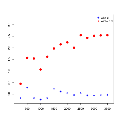
(a) ${\varepsilon}=0.2$

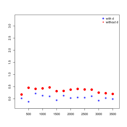
(b) ${\varepsilon}=0.02$

Figure 6: Empirical kurtosis of vector $\bm{v}$ with and without normalization factor ${\sf d}$. In left panel $n=3\,s_{0}$ (with ${\varepsilon}=0.2$, $\delta=0.6$) and in the right panel $n=30\,s_{0}$ (with ${\varepsilon}=0.02$, $\delta=0.6$).

(a) with factor ${\sf d}$

(b) without factor ${\sf d}$

Figure 7: Histogram of $\bm{v}$ for $n=3\,s_{0}$ (${\varepsilon}=0.2$, $\delta=0.6$) and $p=3000$. In left panel, factor ${\sf d}$ is computed by Eq. (27) and in the right panel, ${\sf d}=1$.

(a) with factor ${\sf d}$

(b) without factor ${\sf d}$

Figure 8: Histogram of $\bm{v}$ for $n=30\,s_{0}$ (${\varepsilon}=0.02$, $\delta=0.6$) and $p=3000$. In left panel, factor ${\sf d}$ is computed by Eq. (27) and in the right panel, ${\sf d}=1$.

$\bullet$ $\bf n=30\,s_{0}$

(${\varepsilon}=0.02,\delta=0.6$). Figures 6(b) and 8 show similar plots for this case. As we see, the effect of ${\sf d}$ becomes less noticeable here. The reason is that we expect $\|\bm{\widehat{\theta}}\|_{0}/n=O(s_{0}/n)$, and ${\sf d}=(1-\|\bm{\widehat{\theta}}\|_{0}/n)^{-1}=1+O(s_{0}/n)\approx 1$ for $s_{0}$ much smaller than $n$.

5.3 Comparison with Local Asymptotic Normality

Our approach is based on an asymptotic distributional characterization of the Lasso estimator, cf. Theorem 3.4. Simplifying, the Lasso estimator is in correspondence with a debiased estimator $\bm{\widehat{\theta}}^{u}$ that is asymptotically normal in the sense of finite-dimensional distributions. This is analogous to what happens in classical statistics, where local asymptotic normality (LAN) can be used to characterize an estimator distribution, and hence derive test statistics [56, 57].

This analogy is only superficial, and the mathematical phenomenon underlying Theorem 3.4 is altogether different from the one in local asymptotic normality. We refer to [10] for a more complete understanding, and only mention a few points:

1. LAN theory holds in the low-dimensional limit, where the number of parameters $p$ is much smaller than the number of samples $n$. Even more, the focus is on $p$ fixed, and $n\to\infty$.

   In contrast, the Gaussian limit in Theorem 3.4 holds with $p$ proportional to $n$.

2. The starting point of LAN theory is low-dimensional consistency, namely $\bm{\widehat{\theta}}\to\bm{\theta}_{0}$ as $n\to\infty$. As a consequence, the distribution of $\bm{\widehat{\theta}}$ can be characterized by a local approximation around $\bm{\theta}_{0}$.

   In contrast, in the high-dimensional asymptotic regime of Theorem 3.4, the mean square error per coordinate $\|\bm{\widehat{\theta}}-\bm{\theta}_{0}\|_{2}^{2}/p$ remains bounded away from zero [10]. As a consequence, normality does not follow from local approximation.

3. Indeed, in the present case, the Lasso estimator (which is of course a special case of M-estimator) $\bm{\widehat{\theta}}$ is not normal. Only the debiased estimator $\bm{\widehat{\theta}}^{u}$ is asymptotically normal. Further, while LAN theory holds quite generally in the classical asymptotics, the present theory is more sensitive to the properties of the design matrix ${\bm{X}}$.

6 Real data application

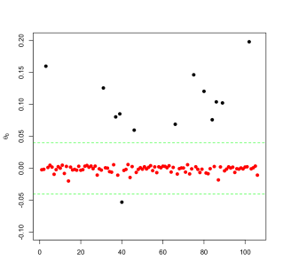
Figure 9: Parameter vector $\bm{\theta}_{0}$ for the communities data set.

We tested our method on the UCI communities and crimes dataset [58]. This concerns the prediction of the rate of violent crime in different communities within US, based on other demographic attributes of the communities. The dataset consists of a response variable along with 122 predictive attributes for 1994 communities. Covariates are quantitative, including e.g., the fraction of urban population or the median family income. We consider a linear model as in (2) and hypotheses $H_{0,i}$. Rejection of $H_{0,i}$ indicates that the $i$-th attribute is significant in predicting the response variable.

We perform the following preprocessing steps: $(i)$ Each missing value is replaced by the mean of the non missing values of that attribute for other communities. $(ii)$ We eliminate $16$ attributes to make the ensemble of the attribute vectors linearly independent. Thus we obtain a design matrix ${\bm{X}}_{\rm tot}\in{\mathbb{R}}^{n_{\rm tot}\times p}$ with $n_{\rm tot}=1994$ and $p=106$; $(iii)$ We normalize each column of the resulting design matrix to have mean zero and $\ell_{2}$ norm equal to $\sqrt{n_{\rm tot}}$.

In order to evaluate various hypothesis testing procedures, we need to know the true significant variables. To this end, we let $\bm{\theta}_{0}=({\bm{X}}_{\rm tot}^{{\sf T}}{\bm{X}}_{\rm tot})^{-1}{\bm{X}}_{\rm tot}^{{\sf T}}{\bm{y}}$ be the least-square estimator, using the whole data set. Figure 9 shows the the entries of $\bm{\theta}_{0}$. Clearly, only a few entries have non negligible values which correspond to the significant attributes. In computing type I errors and powers, we take the elements in $\bm{\theta}_{0}$ with magnitude larger than $0.04$ as active and the others as inactive.

In order to validate our approach in the high-dimensional $p>n$ regime, we take random subsamples of the communities (hence subsamples of the rows of ${\bm{X}}_{\rm tot}$) of size $n=84$. We compare SDL-test  with the method of [17], over $20$ realizations and significance levels $\alpha=0.01,0.025,0.05$. The fraction of type I errors and statistical power is computed by comparing to $\bm{\theta}_{0}$. Table 6 summarizes the results. As the reader can see, Buhlmann’s method is very conservative yielding to no type-I errors and but much smaller power than SDL-test.

In table 7, we report the relevant features obtained from the whole dataset as described above, corresponding to the nonzero entries in $\bm{\theta}_{0}$. We also report the features identified as relevant by SDL-test  and those identified as relevant by Ridge-based regression method, from one random subsample of communities of size $n=84$. Features description is available in [58].

Finally, in Fig. 10 we plot the normalized histograms of $\bm{v}_{S_{0}}$ (in red) and $\bm{V}_{S_{0}^{c}}$ (in white). Recall that $\bm{v}=(v_{i})_{i=1}^{p}$ denotes the vector with $v_{i}\equiv\widehat{\theta}^{u}_{i}/(\tau[(\bm{\Sigma}^{-1})_{ii}]^{1/2})$. Further, $\bm{v}_{S_{0}}$ and $\bm{v}_{S_{0}^{c}}$ respectively denote the restrictions of $\bm{v}$ to the active set $S_{0}$ and the inactive set $S_{0}^{c}$. This plot demonstrates that $\bm{v}_{S^{c}_{0}}$ has roughly standard normal distribution as predicted by the theory.

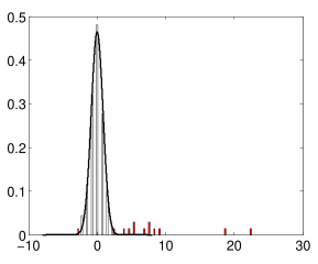
Figure 10: Normalized histogram of $\bm{v}_{S_{0}}$ (in red) and $\bm{v}_{S_{0}^{c}}$ (in white) for the communities data set.

Method	Type I err	Avg. power
	(mean)	(mean)
SDL-test  $(\alpha=0.05)$	0.0172043	0.4807692
Ridge-based regression	0	0.1423077
SDL-test  $(\alpha=0.025)$	0.01129032	0.4230769
Ridge-based regression	0	0.1269231
SDL-test  $(\alpha=0.01)$	0.008602151	0.3576923
Ridge-based regression	0	0.1076923

Table 6: Simulation results for the communities data set.

Relevant features		racePctHisp, PctTeen2Par, PctImmigRecent, PctImmigRec8, PctImmigRec10, PctNotSpeakEnglWell, OwnOccHiQuart, NumStreet, PctSameState85, LemasSwFTFieldPerPop, LemasTotReqPerPop, RacialMatchCommPol, PolicOperBudg
$\alpha=0.01$	Relevant features (SDL-test )	racePctHisp, PctTeen2Par, PctImmigRecent, PctImmigRec8, PctImmigRec10, PctNotSpeakEnglWell, OwnOccHiQuart, NumStreet, PctSameState85, LemasSwFTFieldPerPop, LemasTotReqPerPop, RacialMatchCommPol, PolicOperBudg
	Relevant features (ridge-based regression)	racePctHisp, PctSameState85
$\alpha=0.025$	Relevant features (SDL-test )	racePctHisp, PctTeen2Par, PctImmigRecent, PctImmigRec8, PctImmigRec10, PctNotSpeakEnglWell, PctHousOccup, OwnOccHiQuart, NumStreet, PctSameState85, LemasSwFTFieldPerPop, LemasTotReqPerPop, RacialMatchCommPol, PolicOperBudg
	Relevant features (ridge-based regression)	racePctHisp, PctSameState85
$\alpha=0.05$	Relevant features (SDL-test )	racePctHisp, PctUnemployed, PctTeen2Par, PctImmigRecent, PctImmigRec8, PctImmigRec10, PctNotSpeakEnglWell, PctHousOccup, OwnOccHiQuart, NumStreet, PctSameState85, LemasSwornFT, LemasSwFTFieldPerPop, LemasTotReqPerPop, RacialMatchCommPol, PctPolicWhite
	Relevant features (ridge-based regression)	racePctHisp, PctSameState85

Table 7: The relevant features (using the whole dataset) and the relevant features predicted by SDL-test  and the method of [17] for a random subsample of size $n=84$ from the communities. The false positive predictions are in red.

7 Proofs

7.1 Proof of Lemma 2.6

Fix $\alpha\in[0,1]$, $\mu>0$, and assume that the minimum error rate for type II errors in testing hypothesis $H_{0,i}$ at significance level $\alpha$ is $\beta=\beta^{\rm opt}_{i}(\alpha;\mu)$. Further fix $\xi>0$ arbitrarily small. By definition there exists a statistical test $T_{i,{\bm{X}}}:{\mathbb{R}}^{m}\to\{0,1\}$ such that ${\mathbb{P}}_{\bm{\theta}}(T_{i,{\bm{X}}}({\bm{y}})=1)\leq\alpha$ for any $\bm{\theta}\in{\cal R}_{0}$ and ${\mathbb{P}}_{\bm{\theta}}(T_{i,{\bm{X}}}({\bm{y}})=0)\leq\beta+\xi$ for any $\bm{\theta}\in{\cal R}_{1}$ (with ${\cal R}_{0},{\cal R}_{1}\in{\mathbb{R}}^{p}$ defined as in Definition 2.5). Equivalently:

$$\begin{split}{\mathbb{E}}\big{\{}{\mathbb{P}}_{\bm{\theta}}(T_{i,{\bm{X}}}({\bm{y}})=1|{\bm{X}})\big{\}}&\leq\alpha,\quad\quad\;\;\mbox{for any $\bm{\theta}\in{\cal R}_{0}$,}\\ {\mathbb{E}}\big{\{}{\mathbb{P}}_{\bm{\theta}}(T_{i,{\bm{X}}}({\bm{y}})=0|{\bm{X}})\big{\}}&\leq\beta+\xi,\;\;\;\mbox{for any $\bm{\theta}\in{\cal R}_{1}$.}\end{split}$$ (43)

We now take expectation of these inequalities with respect to $\bm{\theta}\sim Q_{0}$ (in the first case) and $\bm{\theta}\sim Q_{1}$ (in the second case) and we get, with the notation introduced in the Definition 2.5,

$$\begin{split}{\mathbb{E}}\big{\{}{\mathbb{P}}_{Q,0,{\bm{X}}}(T_{i,{\bm{X}}}({\bm{y}})=1)\big{\}}&\leq\alpha\,,\\ {\mathbb{E}}\big{\{}{\mathbb{P}}_{Q,1,{\bm{X}}}(T_{i,{\bm{X}}}({\bm{y}})=0)\big{\}}&\leq\beta+\xi\,.\end{split}$$

Call $\alpha_{{\bm{X}}}\equiv{\mathbb{P}}_{Q,0,{\bm{X}}}(T_{i,{\bm{X}}}({\bm{y}})=1)$. By assumption, for any test $T$, we have ${\mathbb{P}}_{Q,1,{\bm{X}}}(T_{i,{\bm{X}}}({\bm{y}})=0)\geq\beta^{\rm bin}_{i,{\bm{X}}}(\alpha_{{\bm{X}}};Q)$ and therefore the last inequalities imply

$$\begin{split}{\mathbb{E}}\big{\{}\alpha_{{\bm{X}}}\big{\}}&\leq\alpha\,,\\ {\mathbb{E}}\big{\{}\beta^{\rm bin}_{i,{\bm{X}}}(\alpha_{{\bm{X}}};Q)\big{\}}&\leq\beta+\xi\,.\end{split}$$ (44)

The thesis follows since $\xi>0$ is arbitrary.

7.2 Proof of Lemma 2.7

Fix ${\bm{X}}$, $\alpha$, $i$, $S$ as in the statement and assume, without loss of generality, ${\rm{\bf P}}^{\perp}_{S}\bm{\widetilde{x}}_{i}\neq 0$, and ${\rm rank}({\bm{X}}_{S})=|S|<n$. We take $Q_{0}={\sf N}(0,\bm{J})$ where $\bm{J}\in{\mathbb{R}}^{p\times p}$ is the diagonal matrix with $\bm{J}_{jj}=a$ if $j\in S$ and $\bm{J}_{jj}=0$ otherwise. Here $a\in{\mathbb{R}}_{+}$ and will be chosen later. For the same covariance matrix $\bm{J}$, we let $Q_{1}={\sf N}(\mu\,\bm{e}_{i},\bm{J})$ where $\bm{e}_{i}$ is the $i$-th element of the standard basis. Recalling that $i\notin S$, and $|S|<s_{0}$, the support of $Q_{0}$ is in ${\cal R}_{0}$ and the support of $Q_{1}$ is in ${\cal R}_{1}$.

Under ${\mathbb{P}}_{Q,0,{\bm{X}}}$ we have ${\bm{y}}\sim{\sf N}(\bm{0},a\,{\bm{X}}_{S}{\bm{X}}_{S}^{{\sf T}}+\sigma^{2}{\rm I})$, and under ${\mathbb{P}}_{Q,1,{\bm{X}}}$ we have ${\bm{y}}\sim{\sf N}(\mu\bm{\widetilde{x}}_{i},a\,{\bm{X}}_{S}{\bm{X}}_{S}^{{\sf T}}+\sigma^{2}{\rm I})$. Hence the binary hypothesis testing problem under study reduces to the problem of testing a null hypothesis on the mean of a Gaussian random vector with known covariance against a simple alternative. It is well known that the most powerful test [7, Chapter 8] is obtained by comparing the ratio ${\mathbb{P}}_{Q,0,{\bm{X}}}({\bm{y}})/{\mathbb{P}}_{Q,1,{\bm{X}}}({\bm{y}})$ with a threshold. Equivalently, the most powerful test is of the form

$$T_{i,{\bm{X}}}({\bm{y}})={\mathbb{I}}\Big{\{}\langle\mu\bm{\widetilde{x}}_{i},(a{\bm{X}}_{S}{\bm{X}}_{S}^{{\sf T}}+\sigma^{2}{\rm I})^{-1}\bm{y}\rangle\geq c\Big{\}}\,,$$ (45)

for some $c\in{\mathbb{R}}$ that is to be chosen to achieve the desired significance level $\alpha$. Letting

$$\alpha\equiv 2\Phi\Big{(}-\frac{c}{\mu\|(a{\bm{X}}_{S}{\bm{X}}_{S}^{{\sf T}}+\sigma^{2}{\rm I})^{-1/2}\bm{\widetilde{x}}_{i}\|}\Big{)}\,,$$ (46)

it is a straightforward calculation to drive the power of this test as

$$G\Big{(}\alpha,\mu\|(a{\bm{X}}_{S}{\bm{X}}_{S}^{{\sf T}}+\sigma^{2}{\rm I})^{-1/2}\bm{\widetilde{x}}_{i}\|\Big{)}\,,$$

where the function $G(\alpha,u)$ is defined as per Eq. (10). Next we show that the power of this test converges to $1-\beta^{\rm oracle}_{i,{\bm{X}}}(\alpha;S,\mu)$ as $a\to\infty$. Hence the claim is proved by taking $a\geq a(\xi)$ for some $a(\xi)$ large enough.

Write

$$(a{\bm{X}}_{S}{\bm{X}}_{S}^{\sf T}+\sigma^{2}{\rm I})^{-1/2} =\frac{1}{\sigma}\Big{(}{\rm I}+\frac{a}{\sigma^{2}}{\bm{X}}_{S}{\bm{X}}_{S}^{\sf T}\Big{)}^{-1/2}$$

$$=\frac{1}{\sigma}\Big{\{}{\rm I}-{\bm{X}}_{S}\Big{(}\frac{\sigma^{2}}{a}{\rm I}+{\bm{X}}_{S}^{\sf T}{\bm{X}}_{S}\Big{)}^{-1}{\bm{X}}_{S}^{\sf T}\Big{\}}^{1/2}\,,$$ (47)

where the second step follows from matrix inversion lemma. Clearly, as $a\to\infty$, the right hand side of the above equation converges to $(1/\sigma)\,{\rm{\bf P}}^{\perp}_{S}$. Therefore, the power converges to $1-\beta^{\rm oracle}_{i,{\bm{X}}}(\alpha;S,\mu)=G(\alpha,\mu\sigma^{-1}\|{\rm{\bf P}}^{\perp}_{S}\bm{\widetilde{x}}_{i}\|)$.

7.3 Proof of Theorem 2.3

Let $u_{{\bm{X}}}\equiv\mu\|{\rm{\bf P}}^{\perp}_{S}\bm{\widetilde{x}}_{i}\|_{2}/\sigma$. By Lemma 2.6 and 2.7, we have,

$$1-\beta^{\rm opt}_{i}(\alpha;\mu)\leq\sup\Big{\{}{\mathbb{E}}G(\alpha_{\bm{X}},u_{{\bm{X}}})\,:\;\;{\mathbb{E}}(\alpha_{{\bm{X}}})\leq\alpha\Big{\}}\,,$$ (48)

with the $\sup$ taken over measurable functions ${\bm{X}}\mapsto\alpha_{{\bm{X}}}$, and $G(\alpha,u)$ defined as per Eq. (10).

It is easy to check that $\alpha\mapsto G(\alpha,u)$ is concave for any $u\in{\mathbb{R}}_{+}$ and $u\mapsto G(\alpha,u)$ is non-decreasing for any $\alpha\in[0,1]$ (see Fig. LABEL:fig:AlphaBeta1d). Further $G$ takes values in $[0,1]$. Hence

$$\begin{split}{\mathbb{E}}G(\alpha_{\bm{X}},u_{{\bm{X}}})&\leq{\mathbb{E}}\big{\{}G(\alpha_{{\bm{X}}},u_{{\bm{X}}}){\mathbb{I}}(u\leq u_{0})\big{\}}+{\mathbb{P}}(u_{{\bm{X}}}>u_{0})\\ &\leq{\mathbb{E}}\big{\{}G(\alpha_{{\bm{X}}},u_{0})\big{\}}+{\mathbb{P}}(u_{{\bm{X}}}>u_{0})\\ &\leq G({\mathbb{E}}(\alpha_{{\bm{X}}}),u_{0})+{\mathbb{P}}(u_{{\bm{X}}}>u_{0})\\ &\leq G(\alpha,u_{0})+{\mathbb{P}}(u_{{\bm{X}}}>u_{0})\end{split}$$ (49)

Since $\bm{\widetilde{x}}_{i}$ and ${\bm{X}}_{S}$ are jointly Gaussian, we have

$$\bm{\widetilde{x}}_{i}=\bm{\Sigma}_{i,S}\bm{\Sigma}_{S,S}^{-1}{\bm{X}}_{S}+{\Sigma}_{i|S}^{1/2}\bm{z}_{i}\,,$$ (50)

with $\bm{z}_{i}\sim{\sf N}(0,{\rm I}_{n\times n})$ independent of ${\bm{X}}_{S}$. It follows that

$$u_{{\bm{X}}}=(\mu/\sigma)\,{\Sigma}_{i|S}^{1/2}\,\|{\rm{\bf P}}^{\perp}_{S}\bm{z}_{i}\|_{2}\stackrel{{\scriptstyle\rm d}}{{=}}(\mu/\sigma)\,\sqrt{{\Sigma}_{i|S}Z_{n-s_{0}+1}}\,,$$ (51)

with $Z_{n-s_{0}+1}$ a chi-squared random variable with $n-s_{0}+1$ degrees of freedom. The desired claim follows by taking $u_{0}=(\mu/\sigma)\sqrt{{\Sigma}_{i|S}(n-s_{0}+\ell)}$.

7.4 Proof of Theorem 3.3

Since $\{(\bm{\Sigma}(p)={\rm I}_{p\times p},\bm{\theta}_{0}(p),n(p),\sigma(p))\}_{p\in{\mathbb{N}}}$ has a standard distributional limit, the empirical distribution of $\{(\theta_{0,i},\widehat{\theta}^{u}_{i})\}_{i=1}^{p}$ converges weakly to $(\Theta_{0},\Theta_{0}+\tau Z)$ (with probability one). By the portmanteau theorem, and the fact that $\underset{p\to\infty}{\lim\inf}\,\sigma(p)/\sqrt{n(p)}=\sigma_{0}$, we have

$${\mathbb{P}}(0<|\Theta_{0}|<\mu_{0}\sigma_{0})\leq\lim_{p\to\infty}\frac{1}{p}\sum_{i=1}^{p}{\mathbb{I}}\bigg{(}0<\theta_{0,i}<\mu_{0}\frac{\sigma(p)}{\sqrt{n(p)}}\bigg{)}=0.$$ (52)

In addition, since $\mu_{0}\sigma_{0}/2$ is a continuity point of the distribution of $\Theta_{0}$, we have

$$\lim_{p\to\infty}\frac{1}{p}\sum_{i=1}^{p}{\mathbb{I}}(|\theta_{0,i}|\geq\frac{\mu_{0}\sigma_{0}}{2})={\mathbb{P}}(|\Theta_{0}|\geq\frac{\mu_{0}\sigma_{0}}{2}).$$ (53)

Now, by Eq. (52), ${\mathbb{P}}(|\Theta_{0}|\geq\mu_{0}\sigma_{0}/2)={\mathbb{P}}(\Theta_{0}\neq 0)$. Further, ${\mathbb{I}}(|\theta_{0,i}|\geq\mu_{0}\sigma_{0}/2)={\mathbb{I}}(\theta_{0,i}\neq 0)$ for $1\leq i\leq p$, as $p\to\infty$. Therefore, Eq. (53) yields

$$\begin{split}\lim_{p\to\infty}\frac{1}{p}|S_{0}(p)|&=\lim_{p\to\infty}\frac{1}{p}\sum_{i=1}^{p}{\mathbb{I}}(\theta_{0,i}\neq 0)={\mathbb{P}}(\Theta_{0}\neq 0).\end{split}$$ (54)

Hence,

$$\begin{split}\lim_{p\to\infty}\frac{1}{|S_{0}(p)|}\sum_{i\in S_{0}(p)}T_{i,{\bm{X}}}({\bm{y}})&=\lim_{p\to\infty}\frac{1}{|S_{0}(p)|}\sum_{i\in S_{0}(p)}{\mathbb{I}}(P_{i}\leq\alpha)\\ &=\frac{1}{{\mathbb{P}}(\Theta_{0}\neq 0)}\lim_{p\to\infty}\frac{1}{p}\sum_{i=1}^{p}{\mathbb{I}}(P_{i}\leq\alpha,i\in S_{0}(p))\\ &=\frac{1}{{\mathbb{P}}(\Theta_{0}\neq 0)}\lim_{p\to\infty}\frac{1}{p}\sum_{i=1}^{p}{\mathbb{I}}\bigg{(}\Phi^{-1}(1-\alpha/2)\leq\frac{|\widehat{\theta}^{u}_{i}|}{\tau},\,|\theta_{0,i}|\geq\mu_{0}\frac{\sigma(p)}{\sqrt{n(p)}}\bigg{)}\\ &\geq\frac{1}{{\mathbb{P}}(\Theta_{0}\neq 0)}{\mathbb{P}}\bigg{(}\Phi^{-1}(1-\alpha/2)\leq\big{|}\frac{\Theta_{0}}{\tau}+Z\big{|},\,\,|\Theta_{0}|\geq\mu_{0}\sigma_{0}\bigg{)}.\end{split}$$ (55)

Note that $\tau$ depends on the distribution $p_{\Theta_{0}}$. Since $|S_{0}(p)|\leq{\varepsilon}p$, using Eq. (54), we have ${\mathbb{P}}(\Theta_{0}\neq 0)\leq{\varepsilon}$, i.e, $p_{\Theta_{0}}$ is ${\varepsilon}$-sparse. Let $\tilde{\tau}$ denote the maximum $\tau$ corresponding to densities in the family of ${\varepsilon}$-sparse densities. As shown in [32], $\tilde{\tau}=\tau_{*}\sigma_{0}$, where $\tau_{*}$ is defined by Eqs. (22) and (23). Consequently,

$$\begin{split}\lim_{p\to\infty}\frac{1}{|S_{0}(p)|}\sum_{i\in S_{0}(p)}T_{i,{\bm{X}}}({\bm{y}})&\geq{\mathbb{P}}\bigg{(}\Phi^{-1}(1-\alpha/2)\leq\big{|}\frac{\mu_{0}}{\tau_{*}}+Z\big{|}\bigg{)}\\ &=1-{\mathbb{P}}\bigg{(}-\Phi^{-1}(1-\alpha/2)-\frac{\mu_{0}}{\tau_{*}}\leq Z\leq\Phi^{-1}(1-\alpha/2)-\frac{\mu_{0}}{\tau_{*}}\bigg{)}\\ &=1-\{\Phi(\Phi^{-1}(1-\alpha/2)-\mu_{0}/\tau_{*})-\Phi(-\Phi^{-1}(1-\alpha/2)-\mu_{0}/\tau_{*})\}\\ &=G(\alpha,\mu_{0}/\tau_{*})\,.\end{split}$$ (56)

Now, we take the expectation of both sides of Eq. (56) with respect to the law of random design ${\bm{X}}$ and random noise $\bm{w}$. Changing the order of limit and expectation by applying dominated convergence theorem and using linearity of expectation, we obtain

$$\lim_{p\to\infty}\frac{1}{|S_{0}(p)|}\sum_{i\in S_{0}(p)}{\mathbb{E}}_{{\bm{X}},\bm{w}}\{T_{i,{\bm{X}}}({\bm{y}})\}\geq G\Big{(}\alpha,\frac{\mu_{0}}{\tau_{*}}\Big{)}\,.$$ (57)

Since $T_{i,{\bm{X}}}({\bm{y}})$ takes values in $\{0,1\}$, we have ${\mathbb{E}}_{{\bm{X}},\bm{w}}\{T_{i,{\bm{X}}}({\bm{y}})\}={\mathbb{P}}_{\bm{\theta}_{0}(p)}(T_{i,{\bm{X}}}({\bm{y}})=1)$. The result follows by noting that the columns of ${\bm{X}}$ are exchangeable and therefore ${\mathbb{P}}_{\bm{\theta}_{0}(p)}(T_{i,{\bm{X}}}({\bm{y}})=1)$ does not depend on $i$.

7.5 Proof of Theorem 4.3

Since the sequence $\{\bm{\Sigma}(p),\bm{\theta}_{0}(p),n(p),\sigma(p)\}_{p\in{\mathbb{N}}}$ has a standard distributional limit, with probability one the empirical distribution of $\{(\theta_{0,i},\widehat{\theta}^{u}_{i},(\bm{\Sigma}^{-1})_{ii})\}_{i=1}^{p}$ converges weakly to the distribution of $(\Theta_{0},\Theta_{0}+\tau\Upsilon^{1/2}Z,\Upsilon)$. Therefore, with probability one, the empirical distribution of

$$\bigg{\{}\frac{\widehat{\theta}^{u}_{i}-\theta_{0,i}}{\tau[(\bm{\Sigma}^{-1})_{ii}]^{1/2}}\bigg{\}}_{i=1}^{p}$$

converges weakly to ${\sf N}(0,1)$. Hence,

$$\begin{split}\lim_{p\to\infty}\frac{1}{|S_{0}^{c}(p)|}\sum_{i\in S_{0}^{c}(p)}T_{i,{\bm{X}}}({\bm{y}})&=\lim_{p\to\infty}\frac{1}{|S^{c}_{0}(p)|}\sum_{i\in S^{c}_{0}(p)}{\mathbb{I}}(P_{i}\leq\alpha)\\ &=\frac{1}{{\mathbb{P}}(\Theta_{0}=0)}\,\lim_{p\to\infty}\frac{1}{p}\sum_{i=1}^{p}{\mathbb{I}}(P_{i}\leq\alpha,\,i\in S^{c}_{0}(p))\\ &=\frac{1}{{\mathbb{P}}(\Theta_{0}=0)}\,\lim_{p\to\infty}\frac{1}{p}\sum_{i=1}^{p}{\mathbb{I}}\bigg{(}\Phi^{-1}(1-\alpha/2)\leq\frac{|\widehat{\theta}^{u}_{i}|}{\tau[(\bm{\Sigma}^{-1})_{ii}]^{1/2}},\,\theta_{0,i}=0\bigg{)}\\ &=\frac{1}{{\mathbb{P}}(\Theta_{0}=0)}\,{\mathbb{P}}(\Phi^{-1}(1-\alpha/2)\leq|Z|,\Theta_{0}=0)\\ &={\mathbb{P}}(\Phi^{-1}(1-\alpha/2)\leq|Z|)=\alpha.\end{split}$$ (58)

Applying the same argument as in the proof of Theorem 3.3, we obtain the following by taking the expectation of both sides of the above equation

$$\lim_{p\to\infty}\frac{1}{|S_{0}(p)|}\sum_{i\in S_{0}(p)}{\mathbb{P}}_{\bm{\theta}_{0}(p)}(T_{i,{\bm{X}}}({\bm{y}})=1)=\alpha\,.$$ (59)

In particular, for the standard Gaussian design (cf. Theorem 3.2), since the columns of ${\bm{X}}$ are exchangeable we get $\lim_{p\to\infty}{\mathbb{P}}_{\bm{\theta}_{0}(p)}(T_{i,{\bm{X}}}({\bm{y}})=1)=\alpha$ for all $i\in S_{0}(p)$.

7.6 Proof of Theorem 4.4

The proof of Theorem 4.4 proceeds along the same lines as the proof of Theorem 3.3. Since $\{(\bm{\Sigma}(p),\bm{\theta}_{0}(p),n(p),$ $\sigma(p))\}_{p\in{\mathbb{N}}}$ has a standard distributional limit, with probability one the empirical distribution of $\{(\theta_{0,i},\widehat{\theta}^{u}_{i},(\bm{\Sigma}^{-1})_{ii})\}_{i=1}^{p}$ converges weakly to the distribution of $(\Theta_{0},\Theta_{0}+\tau\Upsilon^{1/2}Z,\Upsilon)$. Similar to Eq. (54), we have

$$\lim_{p\to\infty}\frac{1}{p}|S_{0}(p)|={\mathbb{P}}(\Theta_{0}\neq 0).$$ (60)

Also

$$\lim_{p\to\infty}\frac{1}{|S_{0}(p)|}\sum_{i\in S_{0}(p)}T_{i,{\bm{X}}}({\bm{y}}) =\lim_{p\to\infty}\frac{1}{|S_{0}(p)|}\sum_{i\in S_{0}(p)}{\mathbb{I}}(P_{i}\leq\alpha)$$

$$=\frac{1}{{\mathbb{P}}(\Theta_{0}\neq 0)}\lim_{p\to\infty}\frac{1}{p}\sum_{i=1}^{p}{\mathbb{I}}(P_{i}\leq\alpha,i\in S_{0}(p))$$

$$=\frac{1}{{\mathbb{P}}(\Theta_{0}\neq 0)}\lim_{p\to\infty}\frac{1}{p}\sum_{i=1}^{p}{\mathbb{I}}\bigg{(}\Phi^{-1}(1-\alpha/2)\leq\frac{|\widehat{\theta}^{u}_{i}|}{\tau[(\bm{\Sigma}^{-1})_{ii}]^{1/2}},\,\frac{|\theta_{0,i}|}{[(\bm{\Sigma}^{-1})_{ii}]^{1/2}}\geq\mu_{0}\bigg{)}$$

$$=\frac{1}{{\mathbb{P}}(\Theta_{0}\neq 0)}{\mathbb{P}}\bigg{(}\Phi^{-1}(1-\alpha/2)\leq\big{|}\frac{\Theta_{0}}{\tau\Upsilon^{1/2}}+Z\big{|},\,\,\frac{|\Theta_{0}|}{\Upsilon^{1/2}}\geq\mu_{0}\bigg{)}$$

$$\geq\frac{1}{{\mathbb{P}}(\Theta_{0}\neq 0)}{\mathbb{P}}\bigg{(}\Phi^{-1}(1-\alpha/2)\leq\big{|}\frac{\mu_{0}}{\tau}+Z\big{|}\bigg{)}$$

$$=1-\{\Phi(\Phi^{-1}(1-\alpha/2)-\mu_{0}/\tau)-\Phi(-\Phi^{-1}(1-\alpha/2)-\mu_{0}/\tau)\}$$

$$=G(\alpha,\mu_{0}/\tau)\,.$$ (61)

Similar to the proof of Theorem 3.3, by taking the expectation of both sides of the above inequality we get

$$\lim_{p\to\infty}\frac{1}{|S_{0}(p)|}\sum_{i\in S_{0}(p)}{\mathbb{P}}_{\bm{\theta}_{0}}(T_{i,{\bm{X}}}({\bm{y}})=1)\geq G\Big{(}\alpha,\frac{\mu_{0}}{\tau}\Big{)}\,.$$ (62)

7.7 Proof of Theorem 4.5

In order to prove the claim, we will establish the following (corresponding to the the case $\Theta_{0}=0$ of Definition 4.1):

Claim 1.

If $\tau$ solves Eq. (37), then $\tau^{2}\to\sigma^{2}_{0}$ as $p\to\infty$.

Claim 2.

The empirical distribution of $\{(\theta_{0,i},\widehat{\theta}^{u}_{i},(\bm{\Sigma}^{-1})_{ii})\}_{1\leq i\leq p}$ converges weakly to the random vector $(0,\sigma_{0}\Upsilon^{1/2}Z,\Upsilon)$, with $Z\sim{\sf N}(0,1)$ independent of $\Upsilon$. Namely fixing $\psi:{\mathbb{R}}^{3}\to{\mathbb{R}}$, bounded Lipschitz, we need to prove

$$\lim_{p\to\infty}\frac{1}{p}\sum_{i=1}^{p}\psi(\theta_{0,i},\widehat{\theta}^{u}_{i},(\bm{\Sigma}^{-1})_{ii})={\mathbb{E}}\big{\{}\psi(0,\sigma_{0}\Upsilon^{1/2}Z,\Upsilon)\big{\}}\,.$$ (63)

Claim 3.

Recalling $\bm{r}\equiv{\sf d}(\bm{y}-\bm{X}\bm{\widehat{\theta}})/\sqrt{n}$, the empirical distribution of $\{r_{i}\}_{1\leq i\leq n}$ converges weakly to ${\sf N}(0,\sigma_{0}^{2})$.

We will prove these three claims after some preliminary remarks. First notice that, by [59, Theorem 6] (and using assumptions $(i)$ and $(iii)$) ${\bm{X}}$ satisfies the restricted eigenvalue property RE$(s_{0},3s_{0},3)$ of [18] with a $p$-independent constant $\kappa=\kappa(c_{\rm min},c_{\rm max})>0$, almost surely for all $p$ large enough. (Indeed Theorem 6 of [59] ensures that this holds with probability at least $1-e^{-\Omega(n(p))}$, and hence almost surely for all $p$ large enough by Borel-Cantelli lemma.)

We can therefore apply [18, Theorem 7.2] to conclude that there exists a constant $C_{0}$ such that, almost surely for all $p$ large enough, we have

$$\|{\bm{X}}(\bm{\widehat{\theta}}-\bm{\theta}_{0})\|_{2}^{2} \leq\frac{1}{2}\,C_{0}s_{0}\sigma^{2}\log p\leq C_{0}\sigma_{0}^{2}ns_{0}\log p\,,$$ (64)

$$\|\bm{\widehat{\theta}}-\bm{\theta}_{0}\|_{1} \leq\frac{C_{0}s_{0}\sigma}{2}\sqrt{\frac{\log p}{n}}\leq C_{0}\sigma_{0}s_{0}\sqrt{\log p}\,,$$ (65)

$$\|\bm{\widehat{\theta}}-\bm{\theta}_{0}\|_{2}^{2} \leq\frac{C_{0}\sigma^{2}}{2}\,\frac{s_{0}\log p}{n}\leq C_{0}\sigma_{0}^{2}s_{0}\log p\,,$$ (66)

$$\|\bm{\widehat{\theta}}\|_{0} \leq C_{0}s_{0}\,.$$ (67)

(Here we used $\sigma^{2}\leq 2n\sigma_{0}^{2}$ for all $p$ large enough.) In particular, from Eq. (67) and assumption $(i)$, it follows that $\lim_{p\to\infty}\|\widehat{\theta}\|_{0}/n=0$ and hence, almost surely,

$$\lim_{p\to\infty}{\sf d}=1\,.$$ (68)

7.7.1 Claim 1

By Eq. (68), we can assume ${\sf d}\in(1/2,2)$ for all $p$ large enough. By Eq. (37) it is sufficient to show that ${\sf E}_{1}(\tau^{2},b)\to 0$ uniformly for $b\in[1/2,2]$, $\tau\in[0,M\sigma_{0}]$, for some $M\geq 2$. Since $\|\bm{\theta}\|_{0}/p\to 0$, and by dominated convergence, we have

$${\sf E}_{1}(\tau^{2},b) \equiv\lim_{p\to\infty}\frac{1}{p}{\mathbb{E}}\big{\{}\big{\|}\eta_{b}(\tau\bm{\Sigma}^{-1/2}\bm{z})\big{\|}_{\bm{\Sigma}}^{2}\big{\}}\,.$$ (69)

It is easy to see that $\|\eta_{b}(\bm{y})\big{\|}_{\bm{\Sigma}}\leq C\|\bm{y}\|_{2}$ for some constant $C$ depending on $c_{\rm min}$, $c_{\rm max}$. Hence, letting $Y_{p}\equiv\|\eta_{b}(\tau\bm{\Sigma}^{-1/2}\bm{z})\big{\|}_{\bm{\Sigma}}^{2}/p$, we conclude that ${\mathbb{E}}\{Y_{p}^{2}\}$ is bounded uniformly in $p$. By Cauchy-Schwarz

$${\sf E}_{1}(\tau^{2},b) \equiv\lim_{p\to\infty}{\mathbb{E}}\{Y_{p}\}\leq\lim_{p\to\infty}{\mathbb{E}}\{Y_{p}^{2}\}^{1/2}{\mathbb{P}}(Y_{p}\neq 0)^{1/2}\,.$$ (70)

It is therefore sufficient to prove that ${\mathbb{P}}(Y_{p}\neq 0)\to 0$. By definition of $\eta_{b}(\,\cdot\,)$, cf. Eq. (35), we have $\eta_{b}(\bm{y})=0$ if and only if

$$\|\bm{\Sigma}{\bm{y}}\|_{\infty}\leq\frac{\lambda}{b}\,.$$ (71)

Therefore, substituting ${\bm{y}}=\tau\bm{\Sigma}^{-1/2}\bm{z}$, we have

$${\mathbb{P}}(Y_{p}\neq 0)={\mathbb{P}}\Big{(}\|\bm{\Sigma}^{1/2}{\bm{z}}\|_{\infty}>\frac{\lambda}{b\tau}\Big{)}\leq{\mathbb{P}}\Big{(}\max_{i\in[p]}|(\bm{\Sigma}^{1/2}{\bm{z}})_{i}|>\frac{\lambda}{2M\sigma_{0}}\Big{)}\,.$$ (72)

The random variables $(\bm{\Sigma}^{1/2}{\bm{z}})_{i}$ are ${\sf N}(0,\Sigma_{ii})$. Therefore by union bound, since $\Sigma_{ii}\leq c_{\rm max}$, for $Z\sim{\sf N}(0,1)$, we have

$${\mathbb{P}}(Y_{p}\neq 0)\leq p\,{\mathbb{P}}\Big{(}|Z|\geq\frac{\lambda}{2M\sigma_{0}\sqrt{c_{\rm max}}}\Big{)}\leq 2p\exp\Big{(}-\frac{\lambda^{2}}{8M^{2}\sigma_{0}^{2}c_{\max}}\Big{)}\,.$$ (73)

Therefore ${\mathbb{P}}(Y_{p}\neq 0)\to 0$ since $\lambda=C_{*}\sigma_{0}\sqrt{\log p}$, provided $C_{*}\geq M\sqrt{8c_{\max}}$, by Eq. (70).

7.7.2 Claim 2

Let $\bm{z}=\bm{\Sigma}^{-1}{\bm{X}}^{\sf T}\bm{w}/n$. Conditional on ${\bm{X}}$, we have

$$\bm{z}|{\bm{X}}\sim{\sf N}(0,\bm{C}),\quad\bm{C}=\frac{\sigma^{2}}{n}\bm{\Sigma}^{-1}\Big{(}\frac{{\bm{X}}^{\sf T}{\bm{X}}}{n}\Big{)}\bm{\Sigma}^{-1}\,.$$ (74)

Using the assumption $\sigma^{2}/n\to\sigma_{0}^{2}$ and employing [33, Lemma 7.2], we have, almost surely,

$$\lim_{p\to\infty}\max_{i\in[p]}\Big{|}C_{ii}-\sigma^{2}_{0}(\bm{\Sigma}^{-1})_{ii}\Big{|}=0\,.$$ (75)

Consequently, we have, for almost every sequence of matrices ${\bm{X}}$, letting $Z\sim{\sf N}(0,1)$ independent of ${\bm{X}}$

$$\lim_{p\to\infty}\frac{1}{p}\sum_{i=1}^{p}{\mathbb{E}}\big{\{}\psi(0,z_{i},(\bm{\Sigma}^{-1})_{ii})\big{|}{\bm{X}}\big{\}} =\lim_{p\to\infty}\frac{1}{p}\sum_{i=1}^{p}{\mathbb{E}}\big{\{}\psi(0,\sqrt{C_{ii}}Z,(\bm{\Sigma}^{-1})_{ii})\big{|}{\bm{X}}\big{\}}$$ (76)

$$=\lim_{p\to\infty}\frac{1}{p}\sum_{i=1}^{p}{\mathbb{E}}\big{\{}\psi(0,\sigma_{0}\sqrt{(\bm{\Sigma}^{-1})_{ii}}Z,(\bm{\Sigma}^{-1})_{ii})\big{\}}$$ (77)

$$={\mathbb{E}}\big{\{}\psi(0,\sigma_{0}\Upsilon^{1/2}Z,\Upsilon)\big{\}}\,.$$ (78)

(Here, the first identity follows from Eq. (74), the second from Eq. (75) and the Lipschitz continuity of $\psi$, and the last from assumption $(iv)$, together with the fact that $\psi$ is bounded Lipschitz.)

Next, applying Gaussian isoperimetry [60] to the conditional measure of $\bm{z}$ given ${\bm{X}}$ (noting that $\|\bm{C}\|_{2}\leq C_{1}$ almost surely for all $n$ large enough and some constant $C_{1}<\infty$), and to the Lipschitz function $\bm{z}\mapsto\Psi({\bm{z}})\equiv p^{-1}\sum_{i=1}^{p}\psi(0,z_{i},(\bm{\Sigma}^{-1})_{ii})$, we have

$${\mathbb{P}}\Big{\{}|\Psi({\bm{z}})-{\mathbb{E}}\big{(}\Psi({\bm{z}})|{\bm{X}})|\geq{\varepsilon}\Big{|}{\bm{X}}\Big{\}}\leq 2e^{-n{\varepsilon}^{2}/C_{1}}\,,$$ (79)

almost surely for all $n$ large enough. Using Borel-Cantelli lemma, we conclude that, almost surely

$$\lim_{p\to\infty}\frac{1}{p}\sum_{i=1}^{p}\psi(0,z_{i},(\bm{\Sigma}^{-1})_{ii})={\mathbb{E}}\big{\{}\psi(0,\sigma_{0}\Upsilon^{1/2}Z,\Upsilon)\big{\}}\,.$$ (80)

Substituting ${\bm{y}}={\bm{X}}\theta_{0}+\bm{w}$ in definition of $\bm{\widehat{\theta}}^{u}$, we get

$$\bm{\widehat{\theta}}^{u}-\bm{\theta}_{0} =\Big{(}\frac{{\sf d}}{n}\bm{\Sigma}^{-1}{\bm{X}}^{\sf T}{\bm{X}}-{\rm I}\Big{)}(\bm{\theta}_{0}-\bm{\widehat{\theta}})+\frac{{\sf d}}{n}\bm{\Sigma}^{-1}{\bm{X}}^{\sf T}\bm{w}$$

$$={\sf d}\Big{(}\bm{\Sigma}^{-1}\bm{\widehat{\Sigma}}-{\rm I}\Big{)}(\bm{\theta}_{0}-\bm{\widehat{\theta}})+({\sf d}-1)(\bm{\theta}_{0}-\bm{\widehat{\theta}})+\frac{{\sf d}}{n}\bm{\Sigma}^{-1}{\bm{X}}^{\sf T}\bm{w}$$ (81)

$$=\Delta_{1}+\Delta_{2}+{\sf d}\,{\bm{z}}\,,$$ (82)

where we recall that $\bm{\widehat{\Sigma}}\equiv({\bm{X}}^{{\sf T}}{\bm{X}})/n$ and we defined

$$\Delta_{1}={\sf d}\Big{(}\bm{\Sigma}^{-1}\bm{\widehat{\Sigma}}-{\rm I}\Big{)}(\bm{\theta}_{0}-\bm{\widehat{\theta}})\,,\quad\quad\Delta_{2}=({\sf d}-1)(\bm{\theta}_{0}-\bm{\widehat{\theta}})\,.$$ (83)

The proof is therefore concluded if we can show that, almost surely,

$$\lim_{p\to\infty}\frac{1}{p}\sum_{i=1}^{p}\big{|}\psi(\theta_{0,i},\theta_{0,i}+\Delta_{1,i}+\Delta_{2,i}+{\sf d}z_{i},(\bm{\Sigma}^{-1})_{ii})-\psi(0,z_{i},(\bm{\Sigma}^{-1})_{ii})\big{|}=0\,.$$ (84)

In order to simplify the notation, and since the last argument plays no role, we let $\psi_{i}(x,y)\equiv\psi(x,y,(\bm{\Sigma}^{-1})_{ii})$. Without loss of generality we will assume that $\|\psi_{i}\|_{\infty}\leq 1$, and that the Lipschitz modulus of $\psi_{i}$ is at most one.

In order to prove the claim (84), note that, by triangular inequality,

$$\frac{1}{p}\sum_{i=1}^{p}\big{|}\psi_{i}(\theta_{0,i},\theta_{0,i}+ \Delta_{1,i}+\Delta_{2,i}+{\sf d}z_{i})-\psi_{i}(0,z_{i})\big{|}$$ (85)

$$\leq\frac{1}{p}\sum_{i=1}^{p}g(\theta_{0,i})+\frac{1}{p}\sum_{i=1}^{p}g(\Delta_{1,i})+\frac{1}{p}\sum_{i=1}^{p}g(\Delta_{2,i})+\frac{1}{p}\sum_{i=1}^{p}g\big{(}|{\sf d}-1|\,z_{i}\big{)}\,,$$ (86)

where $g(x)\equiv\min(|x|,2)$.

The first term in Eq. (86) vanishes since by assumption $(i)$, $s_{0}\leq n/(\log p)^{2}$, and therefore

$$\lim_{p\to\infty}\frac{1}{p}\sum_{i=1}^{p}g(\theta_{0,i})\leq\lim_{p\to\infty}\frac{2s_{0}}{p}=0\,.$$ (87)

Consider next the third term in Eq. (86):

$$\frac{1}{p}\sum_{i=1}^{p}g(\Delta_{2,i})\leq\frac{1}{p}\,|{\sf d}-1|\,\|\bm{\widehat{\theta}}-\bm{\theta}_{0}\|_{1}\leq\frac{1}{p}\,|{\sf d}-1|\,C_{0}\sigma_{0}s_{0}\sqrt{\log p}\,,$$ (88)

where the second inequality follows from (65), that holds almost surely for all $p$ large enough. Next, using Eq. (68),

$$\lim_{p\to\infty}\frac{1}{p}\sum_{i=1}^{p}g(\Delta_{2,i})=0\,.$$ (89)

Consider next the last term in Eq. (86), and fix $\delta>0$ arbitrarily small. Since by Eq. (68), $|{\sf d}-1|\leq\delta$ almost surely for all $p$ large enough, we have

$$\lim\sup_{p\to\infty}\frac{1}{p}\sum_{i=1}^{p}g\big{(}|{\sf d}-1|\,z_{i}\big{)}\leq\lim\sup_{p\to\infty}\frac{1}{p}\sum_{i=1}^{p}g\big{(}\delta\,z_{i}\big{)}={\mathbb{E}}\{g(\delta\sigma_{0}\Upsilon^{1/2}Z)\}\,,$$ (90)

where the last equality follows from Eq. (80), applied to $\psi(a,b,c)=g(\delta b)$. Finally, letting $\delta\to 0$, we get, by dominated convergence, $\lim_{\delta\to 0}{\mathbb{E}}\{g(\delta\sigma_{0}\Upsilon^{1/2}Z)\}=0$, and hence

$$\lim\sup_{p\to\infty}\frac{1}{p}\sum_{i=1}^{p}g\big{(}|{\sf d}-1|\,z_{i}\big{)}=0\,.$$ (91)

Finally, consider the second term. Fix a partition $[p]=\cup_{\ell=1}^{L}A_{\ell}$, where $s_{0}\leq|A_{\ell}|\leq 9\,s_{0}$, and $p/(9s_{0})\leq L\leq(p/s_{0})$. Then

$$\frac{1}{p}\sum_{i=1}^{p}g(\Delta_{1,i})\leq\frac{1}{p}\|\Delta_{1}\|_{1} \leq\frac{1}{p}\sum_{\ell=1}^{L}\sqrt{|A_{\ell}|}\,\|\Delta_{1,A_{\ell}}\|_{2}\leq\frac{3}{\sqrt{s_{0}}}\max_{1\leq\ell\leq L}\,\|\Delta_{1,A_{\ell}}\|_{2}\,.$$ (92)

Let $T\equiv{\rm supp}(\bm{\widehat{\theta}})\cup{\rm supp}(\bm{\theta}_{0})$. By Eq. (67) we have $|T|\leq(C_{0}+1)s_{0}$ almost surely for all $p$ large enough. Hence, using ${\sf d}\leq 2$ for all $p$ large enough, we get

$$\|\Delta_{1,A_{\ell}}\|_{2}\leq 2\big{\|}\big{(}\bm{\Sigma}^{-1}\bm{\widehat{\Sigma}}-{\rm I}\big{)}_{A_{\ell},T}\big{\|}_{2}\|\bm{\widehat{\theta}}-\bm{\theta}_{0}\|_{2}\,.$$ (93)

The operator norm can be upper bounded using the following lemma, whose proof can be found in Appendix G. (See also the conference paper [33] for a similar estimate: we provide a full proof in appendix for the reader’s convenience.)

Lemma 7.1.

Under the assumption of Theorem 4.5, for any constant $c_{0}$, there exists $K=K(c_{\rm min},c_{\rm max},c_{0})$

$$\max\Big{\{}\big{\|}\big{(}\bm{\Sigma}^{-1}\bm{\widehat{\Sigma}}-{\rm I}\big{)}_{A,B}\big{\|}_{2}:\;A,B\subseteq[p],\;|A|,|B|\leq c_{0}\,s_{0}\Big{\}}\leq K\,\sqrt{\frac{s_{0}\log p}{n}}\,,$$ (94)

with probability at least $(1-p^{-5})$ for all $p$ large enough.

Using Borel-Cantelli lemma together with Eq. (94) and Eq. (66) in Eq. (93) we get, almost surely for all $p$ large enough, and some constant $C$

$$\|\Delta_{1,A_{\ell}}\|_{2}\leq C\sigma_{0}\frac{s_{0}\log p}{\sqrt{n}}\,$$ (95)

Hence, using Eq. (92) and assumption $(i)$

$$\lim_{p\to\infty}\frac{1}{p}\sum_{i=1}^{p}g(\Delta_{1,i})\leq\lim_{p\to\infty}C^{\prime}\sigma_{0}\frac{\sqrt{s_{0}}\log p}{\sqrt{n}}=0\,.$$ (96)

This finishes the proof of Claim 2.

7.7.3 Claim 3

Note that, by definition

$$\bm{r}=\frac{1}{\sqrt{n}}\bm{w}+\frac{{\sf d}}{\sqrt{n}}\,\bm{X}(\bm{\theta}_{0}-\bm{\widehat{\theta}})+\frac{{\sf d}-1}{\sqrt{n}}\bm{w}\,.$$ (97)

Defining ${\bm{u}}\equiv\bm{w}/\sqrt{n}$, ${\bm{h}}_{1}\equiv{\sf d}\bm{X}(\bm{\theta}_{0}-\bm{\widehat{\theta}})/\sqrt{n}$, and ${\bm{h}}_{2}\equiv({\sf d}-1){\bm{u}}$, the proof consists in two steps. First, for any Lipschitz bounded function $\psi:{\mathbb{R}}\to{\mathbb{R}}$, we have

$$\lim_{p\to\infty}\frac{1}{n}\sum_{i=1}^{n}\psi(u_{i})={\mathbb{E}}\{\psi(\sigma_{0}\,Z)\}\,.$$ (98)

This is immediate by the law of large numbers, since ${\bm{u}}$ has i.i.d. ${\sf N}(0,\sigma^{2}/n)$ entries and by assumption $\sigma^{2}/n\to\sigma_{0}^{2}$.

Second, we have

$$\frac{1}{n}\sum_{i=1}^{n}\big{|}\psi(r_{i})-\psi(u_{i})\big{|}\leq\frac{1}{n}\sum_{i=1}^{n}g(h_{1,i})+\frac{1}{n}\sum_{i=1}^{n}g(h_{2,i})\,,$$ (99)

and the right hand side converges to $0$ as $p\to\infty$. Here the first term is controlled using Eq. (64), and the second using Eq. (68). These derivations are almost identical to the ones of Claim 2, and we omit them.

Appendix A Effective noise variance $\tau_{0}^{2}$

As stated in Theorem 3.4 the unbiased estimator $\bm{\widehat{\theta}}^{u}$ can be regarded –asymptotically– as a noisy version of $\bm{\theta}_{0}$ with noise variance $\tau_{0}^{2}$. An explicit formula for $\tau_{0}$ is given in [10]. For the reader’s convenience, we explain it here using our notations.

Denote by $\eta:{\mathbb{R}}\times{\mathbb{R}}_{+}\to{\mathbb{R}}$ the soft thresholding function

$$\eta(x;a)=\begin{cases}x-a&\text{if }x>a,\\ 0&\text{if }-a\leq x\leq a\\ x+a&\text{otherwise.}\end{cases}$$ (100)

Further define function ${\sf F}:{\mathbb{R}}_{+}\times{\mathbb{R}}_{+}\to{\mathbb{R}}_{+}$ as

$${\sf F}(\tau^{2},a)=\sigma^{2}+\frac{1}{\delta}{\mathbb{E}}\{[\eta(\Theta_{0}+\tau Z;a)-\Theta_{0}]^{2}\}\,,$$ (101)

where $\Theta_{0}$ and $Z$ are defined as in Theorem 3.4. Let $\kappa_{\min}=\kappa_{\min}(\delta)$ be the unique non-negative solution of the equation

$$(1+\kappa^{2})\Phi(-\kappa)-\kappa\phi(\kappa)=\frac{\delta}{2}\,.$$ (102)

The effective noise variance $\tau_{0}^{2}$ is obtained by solving the following two equations for $\kappa$ and $\tau$, restricted to the interval $\kappa\in(\kappa_{\min},\infty)$:

$$\tau^{2} = {\sf F}(\tau^{2},\kappa\tau)\,,$$ (103)

$$\lambda = \kappa\tau\bigg{[}1-\frac{1}{\delta}{\mathbb{P}}(|\Theta_{0}+\tau Z|\geq\kappa\tau)\bigg{]}\,.$$ (104)

Existence and uniqueness of $\tau_{0}$ is proved in [10, Proposition 1.3].

Appendix B Tunned regularization parameter $\lambda$

In previous appendix, we provided the value of $\tau_{0}$ for a given regularization parameter $\lambda$. In this appendix, we discuss the tuned value for $\lambda$ to achieve the power stated in Theorem 3.3.

Let ${\cal F}_{{\varepsilon}}\equiv\{p_{\Theta_{0}}:\,\,\,p_{\Theta_{0}}(\{0\})\geq 1-{\varepsilon}\}$ be the family of ${\varepsilon}$-sparse distributions. Also denote by ${M}({\varepsilon},\kappa)$ the minimax risk of soft thresholding denoiser (at threshold value $\kappa$) over ${\cal F}_{\varepsilon}$, i.e.,

$$M({\varepsilon},\kappa)=\sup_{p_{\Theta_{0}}\in{\cal F}_{\varepsilon}}\,{\mathbb{E}}\{[\eta(\Theta_{0}+Z;\kappa)-\Theta_{0}]^{2}\}\,.$$ (105)

The function $M$ can be computed explicitly by evaluating the mean square error on the worst case ${\varepsilon}$-sparse distribution. A simple calculation gives

$${M}({\varepsilon},\kappa)={\varepsilon}(1+\kappa^{2})+(1-{\varepsilon})[2(1+\kappa^{2})\Phi(-\kappa)-2\kappa\phi(\kappa)]\,.$$ (106)

Further, let

$$\kappa_{*}({\varepsilon})\equiv\arg\min_{\kappa\in{\mathbb{R}}_{+}}{M}({\varepsilon},\kappa)\,.$$ (107)

In words, $\kappa_{*}({\varepsilon})$ is the minimax optimal value of threshold $\kappa$ over ${\cal F}_{\varepsilon}$. The value of $\lambda$ for Theorem 3.3 is then obtained by solving Eq. (103) for $\tau$ with $\kappa=\kappa_{*}({\varepsilon})$, and then substituting $\kappa_{*}$ and $\tau$ in Eq. (104) to get $\lambda=\lambda(p_{\Theta_{0}},\sigma,{\varepsilon},\delta)$.

Remark B.1.

The theory of [10, 11] implies that in the standard Gaussian setting and for a converging sequence of instances $\{(\bm{\theta}_{0}(p),n(p),\sigma(p))\}_{p\in{\mathbb{N}}}$, Eq. (104) is equivalent to the following:

$$\lambda{\sf d}=\kappa\tau\,,$$ (108)

where the normalization factor ${\sf d}$ is given by Eq. (17).

Appendix C Statistical power of earlier approaches

In this appendix, we briefly compare our results with those of Zhang and Zhang [16], and Bühlmann [17]. Both of these papers consider deterministic designs under restricted eigenvalue conditions. As a consequence, controlling both type I and type II errors requires a significantly larger value of $\mu/\sigma$.

In [16], authors propose low dimensional projection estimator (LDPE ) to assess confidence intervals for the parameters $\theta_{0,j}$. Following the treatment of [16], a necessary condition for rejecting $H_{0,j}$ with non-negligible probability is

$$|\theta_{0,j}|\geq c\tau_{j}\sigma(1+\epsilon^{\prime}_{n}),$$ (109)

which follows immediately from [16, Eq. (23)]. Further $\tau_{j}$ and ${\varepsilon}^{\prime}_{n}$ are lower bounded in [16] as follows

$$\tau_{j} \geq\frac{1}{\|\bm{\widetilde{x}}_{j}\|_{2}}\,,$$ (110)

$${\varepsilon}^{\prime}_{n} \geq C\eta^{*}s_{0}\sqrt{\frac{\log p}{n}}\,,$$ (111)

where for a standard Gaussian design $\eta^{*}\geq\sqrt{\log p}$. Using further $\|\bm{\widetilde{x}}_{j}\|_{2}\leq 2\sqrt{n}$ which again holds with high probability for standard Gaussian designs, we get the necessary condition

$$|\theta_{0,j}|\geq c^{\prime}\max\Big{\{}\frac{\sigma s_{0}\log p}{n},\frac{\sigma}{\sqrt{n}}\Big{\}}\,,$$ (112)

for some constant $c^{\prime}$.

In [17], p-values are defined, in the notation of the present paper, as

$$P_{j}\equiv 2\Big{\{}1-\Phi\big{(}(a_{n,p;j}(\sigma)|\widehat{\theta}_{j,{\rm corr}}|-\Delta_{j})_{+}\big{)}\Big{\}}\,,$$ (113)

with $\widehat{\theta}_{j,{\rm corr}}$ a ‘corrected’ estimate of $\theta_{0,j}$, cf. [17, Eq. (2.14)]. The corrected estimate $\widehat{\theta}_{j,{\rm corr}}$ is defined by the following motivation. The ridge estimator bias, in general, can be decomposed into two terms. The first term is the estimation bias governed by the regularization, and the second term is the additional projection bias ${\rm{\bf P}}_{{\bm{X}}}\bm{\theta}_{0}-\bm{\theta}_{0}$, where ${\rm{\bf P}}_{{\bm{X}}}$ denotes the orthogonal projector on the row space of ${\bm{X}}$. The corrected estimate $\widehat{\theta}_{j,{\rm corr}}$ is defined in such a way to remove the second bias term under the null hypothesis $H_{0,j}$. Therefore, neglecting the first bias term, we have $\widehat{\theta}_{j,{\rm corr}}=({\rm{\bf P}}_{{\bm{X}}})_{jj}\theta_{0,j}$.

Assuming the corrected estimate to be consistent (which it is in $\ell_{1}$ sense under the assumption of the paper), rejecting $H_{0,j}$ with non-negligible probability requires

$$|\theta_{0,j}|\geq\frac{c}{a_{n,p;j}(\sigma)|({\rm{\bf P}}_{{\bm{X}}})_{jj}|}\max\{\Delta_{j},1\}\,,$$ (114)

Following [17, Eq. (2.13)] and keeping the dependence on $s_{0}$ instead of assuming $s_{0}=o((n/\log p)^{\xi})$, we have

$$\frac{\Delta_{j}}{a_{n,p;j}(\sigma)|({\rm{\bf P}}_{{\bm{X}}})_{jj}|}=C\max_{k\in[p]\backslash j}\frac{|({\rm{\bf P}}_{{\bm{X}}})_{jk}|}{|({\rm{\bf P}}_{{\bm{X}}})_{jj}|}\,\sigma s_{0}\sqrt{\frac{\log p}{n}}\,.$$ (115)

Further, plugging for $a_{n,p;j}$ we have

$$\frac{1}{a_{n,p;j}(\sigma)|({\rm{\bf P}}_{{\bm{X}}})_{jj}|}=\frac{\sigma\sqrt{\Omega_{jj}}}{\sqrt{n}\,|({\rm{\bf P}}_{{\bm{X}}})_{jj}|}\,.$$ (116)

For a standard Gaussian design $(p/n)({\rm{\bf P}}_{{\bm{X}}})_{jk}$ is approximately distributed as $u_{1}$, where $\bm{u}=(u_{1},u_{2},\dots,$ $u_{n})\in{\mathbb{R}}^{n}$ is a uniformly random vector with $\|\bm{u}\|=1$. In particular $u_{1}$ is approximately ${\sf N}(0,1/n)$. A standard calculation yields $\max_{k\in[p]\setminus j}|({\rm{\bf P}}_{{\bm{X}}})_{jk}|\geq\sqrt{n\log p}/p$ with high probability. Furthermore, $|({\rm{\bf P}}_{{\bm{X}}})_{jj}|$ concentrates around $n/p$. Finally, by definition of $\Omega_{jj}$ (cf. [17, Eq. (2.3)]) and using classical large deviation results about the singular values of a Gaussian matrix, we have $\Omega_{jj}\geq(n/p)^{2}$ with high probability. Hence, a necessary condition for rejecting $H_{0,j}$ with non-negligible probability is

$$|\theta_{0,j}|\geq C\max\Big{\{}\frac{\sigma s_{0}\log p}{n},\frac{\sigma}{\sqrt{n}}\Big{\}},$$ (117)

as stated in Section 1.

Appendix D Replica method calculation

In this section we outline the replica calculation leading to the Claim 4.6. Indeed we consider an even more general setting, whereby the $\ell_{1}$ regularization is replaced by an arbitrary separable penalty. Namely, instead of the Lasso, we consider regularized least squares estimators of the form

$$\bm{\widehat{\theta}}({\bm{y}},{\bm{X}})=\arg\min_{\bm{\theta}\in{\mathbb{R}}^{p}}\Big{\{}\frac{1}{2n}\|{\bm{y}}-{\bm{X}}\bm{\theta}\|^{2}+J(\bm{\theta})\Big{\}}\,,$$ (118)

with $J(\bm{\theta})$ being a convex separable penalty function; namely for a vector $\bm{\theta}\in{\mathbb{R}}^{p}$, we have $J(\bm{\theta})=J_{1}(\theta_{1})+\cdots+J_{p}(\theta_{p})$, where $J_{\ell}:{\mathbb{R}}\to{\mathbb{R}}$ is a convex function. Important instances from this ensemble of estimators are Ridge-regression ($J(\bm{\theta})=\lambda\|\bm{\theta}\|^{2}/2$), and the Lasso ($J(\bm{\theta})=\lambda\|\bm{\theta}\|_{1}$). The Replica Claim 4.6 is generalized to the present setting replacing $\lambda\|\bm{\theta}\|_{1}$ by $J(\bm{\theta})$. The only required modification concerns the definition of the factor ${\sf d}$. We let ${\sf d}$ be the unique positive solution of the following equation

$$1=\frac{1}{{\sf d}}+\frac{1}{n}\,{\rm Trace}\Big{\{}({\rm I}+{\sf d}\bm{\Sigma}^{-1/2}\nabla^{2}J(\bm{\widehat{\theta}})\bm{\Sigma}^{-1/2})^{-1}\Big{\}},$$ (119)

where $\nabla^{2}J(\bm{\widehat{\theta}})$ denotes the Hessian, which is diagonal since $J$ is separable. If $J$ is non differentiable, then we formally set $[\nabla^{2}J(\bm{\widehat{\theta}})]_{ii}=\infty$ for all the coordinates $i$ such that $J$ is non-differentiable at $\widehat{\theta}_{i}$. It can be checked that this definition is well posed and that yields the previous choice for $J(\bm{\theta})=\lambda\|\bm{\theta}\|_{1}$.

We pass next to establishing the claim. We limit ourselves to the main steps, since analogous calculations can be found in several earlier works [40, 41, 48]. For a general introduction to the method and its motivation we refer to [61, 62]. Also, for the sake of simplicity, we shall focus on characterizing the asymptotic distribution of $\bm{\widehat{\theta}}^{u}$, cf. Eq. (28). The distribution of $r$ is derived by the same approach.

Fix a sequence of instances $\{(\bm{\Sigma}(p),\bm{\theta}_{0}(p),n(p),\sigma(p))\}_{p\in{\mathbb{N}}}$. For the sake of simplicity, we assume $\sigma(p)^{2}=n(p)\sigma_{0}^{2}$ and $n(p)=p\delta$ (the slightly more general case $\sigma(p)^{2}=n(p)[\sigma_{0}^{2}+o(1)]$ and $n(p)=p[\delta+o(1)]$ does not require any change to the derivation given here, but is more cumbersome notationally). Fix $\widetilde{g}:{\mathbb{R}}\times{\mathbb{R}}\times{\mathbb{R}}\to{\mathbb{R}}$ a continuous function convex in its first argument, and let $g(u,y,z)\equiv\max_{x\in{\mathbb{R}}}[ux-\widetilde{g}(x,y,z)]$ be its Lagrange dual. The replica calculation aims at estimating the following moment generating function (partition function)

$${\cal Z}_{p}(\beta,s)\equiv\int\!\exp\Big{\{}-\frac{\beta}{2n}\|{\bm{y}}-{\bm{X}}\bm{\theta}\|_{2}^{2}-\beta J(\bm{\theta}) -\beta s\sum_{i=1}^{p}[g(u_{i},\theta_{0,i},(\bm{\Sigma}^{-1})_{ii})-u_{i}\widehat{\theta}^{u}_{i}]$$

$$-\frac{\beta}{2n}(s\tilde{\sf d})^{2}\|{\bm{X}}\bm{\Sigma}^{-1}\bm{u}\|^{2}_{2}\Big{\}}{\rm d}\bm{\theta}\,{\rm d}\bm{u}\,.$$ (120)

Here $(y_{i},\bm{x}_{i})$ are i.i.d. pairs distributed as per model (1) and $\bm{\widehat{\theta}}^{u}=\bm{\theta}+(\tilde{\sf d}/n)\,\bm{\Sigma}^{-1}{\bm{X}}^{\sf T}({\bm{y}}-{\bm{X}}\bm{\theta})$ with $\tilde{\sf d}\in{\mathbb{R}}$ to be defined below. Further, $g:{\mathbb{R}}\times{\mathbb{R}}\times{\mathbb{R}}\to{\mathbb{R}}$ is a continuous function strictly convex in its first argument. Finally, $s\in{\mathbb{R}}_{+}$ and $\beta>0$ is a ‘temperature’ parameter not to be confused with the type II error rate as used in the main text. We will eventually show that the appropriate choice of $\tilde{\sf d}$ is given by Eq. (119).

Within the replica method, it is assumed that the limits $p\to\infty$, $\beta\to\infty$ exist almost surely for the quantity $(p\beta)^{-1}\log{\cal Z}_{p}(\beta,s)$, and that the order of the limits can be exchanged. We therefore define

$${\mathfrak{F}}(s) \equiv -\lim_{\beta\to\infty}\lim_{p\to\infty}\frac{1}{p\beta}\,\log{\cal Z}_{p}(\beta,s)$$ (121)

$$\equiv -\lim_{p\to\infty}\lim_{\beta\to\infty}\frac{1}{p\beta}\,\log{\cal Z}_{p}(\beta,s)\,.$$ (122)

In other words ${\mathfrak{F}}(s)$ is the exponential growth rate of ${\cal Z}_{p}(\beta,s)$. It is also assumed that $p^{-1}\log{\cal Z}_{p}(\beta,s)$ concentrates tightly around its expectation so that ${\mathfrak{F}}(s)$ can in fact be evaluated by computing

$${\mathfrak{F}}(s)=-\lim_{\beta\to\infty}\lim_{p\to\infty}\frac{1}{p\beta}\,{\mathbb{E}}\log{\cal Z}_{p}(\beta,s)\,,$$ (123)

where expectation is being taken with respect to the distribution of $(y_{1},\bm{x}_{1}),\cdots,(y_{n},\bm{x}_{n})$. Notice that, by Eq. (122) and using Laplace method in the integral (120), we have

$${\mathfrak{F}}(s)=$$

$$\lim_{p\to\infty}\frac{1}{p}\min_{\bm{\theta},\bm{u}\in{\mathbb{R}}^{p}}\Big{\{}\frac{1}{2n}\|{\bm{y}}-{\bm{X}}\bm{\theta}\|_{2}^{2}+J(\bm{\theta})+s\sum_{i=1}^{p}[g(u_{i},\theta_{0,i},(\bm{\Sigma}^{-1})_{ii})-u_{i}\widehat{\theta}^{u}_{i}]+\frac{1}{2n}(s\tilde{\sf d})^{2}\|{\bm{X}}\bm{\Sigma}^{-1}\bm{u}\|^{2}_{2}\Big{\}}.$$ (124)

Finally we assume that the derivative of ${\mathfrak{F}}(s)$ as $s\to 0$ can be obtained by differentiating inside the limit. This condition holds, for instance, if the cost function is strongly convex at $s=0$. We get

$$\frac{{\rm d}{\mathfrak{F}}}{{\rm d}s}(s=0)=\lim_{p\to\infty}\frac{1}{p}\sum_{i=1}^{p}\min_{u_{i}\in{\mathbb{R}}}[g(u_{i},\theta_{0,i},(\bm{\Sigma}^{-1})_{ii})-u_{i}\widehat{\theta}^{u}_{i}]$$ (125)

where $\bm{\widehat{\theta}}^{u}=\bm{\widehat{\theta}}+(\tilde{\sf d}/n)\,\bm{\Sigma}^{-1}{\bm{X}}^{\sf T}({\bm{y}}-{\bm{X}}\bm{\widehat{\theta}})$ and $\bm{\widehat{\theta}}$ is the minimizer of the regularized least squares as per Eq. (4). Since, by duality $\widetilde{g}(x,y,z)\equiv\max_{u\in{\mathbb{R}}}[ux-g(u,y,z)]$, we get

$$\frac{{\rm d}{\mathfrak{F}}}{{\rm d}s}(s=0) =-\lim_{p\to\infty}\frac{1}{p}\sum_{i=1}^{p}\widetilde{g}(\widehat{\theta}^{u}_{i},\theta_{0,i},(\bm{\Sigma}^{-1})_{ii})\,.$$ (126)

Hence, by computing ${\mathfrak{F}}(s)$ using Eq. (123) for a complete set of functions $\widetilde{g}$, we get access to the corresponding limit quantities (126) and hence, via standard weak convergence arguments, to the joint empirical distribution of the triple $(\widehat{\theta}^{u}_{i},\theta_{0,i},(\bm{\Sigma}^{-1})_{ii})$, cf. Eq. (29).

In order to carry out the calculation of ${\mathfrak{F}}(s)$, we begin by rewriting the partition function (120) in a more convenient form. Using the definition of $\bm{\widehat{\theta}}^{u}$ and after a simple manipulation

$${\cal Z}_{p}(\beta,s)=$$

$$\int\!\exp\Big{\{}-\frac{\beta}{2n}\|{\bm{y}}-{\bm{X}}(\bm{\theta}+s\tilde{\sf d}\bm{\Sigma}^{-1}\bm{u})\|_{2}^{2}-\beta J(\bm{\theta})+\beta s\langle\bm{u},\bm{\theta}\rangle-\beta\,s\sum_{i=1}^{p}g(u_{i},\theta_{0,i},(\bm{\Sigma}^{-1})_{ii})\Big{\}}{\rm d}\bm{\theta}\,{\rm d}\bm{u}\,.$$ (127)

Define the measure $\nu({\rm d}\bm{\theta})$ over $\bm{\theta}\in{\mathbb{R}}^{p}$ as follows

$$\nu({\rm d}\bm{\theta})=\int\exp\Big{\{}-\beta J(\bm{\theta}-s\tilde{\sf d}\bm{\Sigma}^{-1}\bm{u})+\beta s\langle\bm{\theta}-s\tilde{\sf d}\bm{\Sigma}^{-1}\bm{u},\bm{u}\rangle-\beta s\sum_{i=1}^{p}g(u_{i},\theta_{0,i},(\bm{\Sigma}^{-1})_{ii})\Big{\}}\,{\rm d}\bm{u}\,.$$ (128)

Using this definition and with the change of variable $\bm{\theta}^{\prime}=\bm{\theta}+s\tilde{\sf d}\bm{\Sigma}^{-1}\bm{u}$, we can rewrite Eq. (127) as

$${\cal Z}_{p}(\beta,s) \equiv\int\!\exp\Big{\{}-\frac{\beta}{2n}\|{\bm{y}}-{\bm{X}}\bm{\theta}\|_{2}^{2}\Big{\}}\,\nu({\rm d}\bm{\theta})$$

$$=\int\!\exp\Big{\{}i\sqrt{\frac{\beta}{n}}\langle\bm{z},{\bm{y}}-{\bm{X}}\bm{\theta}\rangle\Big{\}}\,\nu({\rm d}\bm{\theta})\,\gamma_{n}({\rm d}\bm{z})$$

$$=\int\!\exp\Big{\{}i\sqrt{\frac{\beta}{n}}\langle\bm{w},\bm{z}\rangle+i\sqrt{\frac{\beta}{n}}\langle\bm{z},{\bm{X}}(\bm{\theta}_{0}-\bm{\theta})\rangle\Big{\}}\,\nu({\rm d}\bm{\theta})\,\gamma({\rm d}\bm{z})\,,$$ (129)

where $\gamma_{n}({\rm d}\bm{z})$ denotes the standard Gaussian measure on ${\mathbb{R}}^{n}$: $\gamma_{n}({\rm d}\bm{z})\equiv(2\pi)^{-n/2}\exp(-\|\bm{z}\|^{2}_{2}/2)\,{\rm d}\bm{z}$.

The replica method aims at computing the expected log-partition function, cf. Eq. (123) using the identity

$${\mathbb{E}}\log{\cal Z}_{p}(\beta,s)=\left.\frac{{\rm d}\phantom{k}}{{\rm d}k}\right|_{k=0}\log{\mathbb{E}}\big{\{}{\cal Z}_{p}(\beta,s)^{k}\big{\}}\,.$$ (130)

This formula would require computing fractional moments of ${\cal Z}_{p}$ as $k\to 0$. The replica method consists in a prescription that allows to compute a formal expression for the $k$ integer, and then extrapolate it as $k\to 0$. Crucially, the limit $k\to 0$ is inverted with the one $p\to\infty$:

$$\lim_{p\to\infty}\frac{1}{p}{\mathbb{E}}\log{\cal Z}_{p}(\beta,s)=\left.\frac{{\rm d}\phantom{k}}{{\rm d}k}\right|_{k=0}\lim_{p\to\infty}\frac{1}{p}\log{\mathbb{E}}\big{\{}{\cal Z}_{p}(\beta,s)^{k}\big{\}}\,.$$ (131)

In order to represent ${\cal Z}_{p}(\beta,s)^{k}$, we use the identity

$$\Big{(}\int f(\bm{x})\,\rho({\rm d}\bm{x})\Big{)}^{k}=\int f(\bm{x}^{1})f(\bm{x}^{2})\cdots f(\bm{x}^{k})\,\rho({\rm d}\bm{x}^{1})\cdots\rho({\rm d}\bm{x}^{k})\,.$$ (132)

In order to apply this formula to Eq. (129), we let, with a slight abuse of notation, $\nu^{k}({\rm d}\bm{\theta})\equiv\nu({\rm d}\bm{\theta}^{1})\times\nu({\rm d}\bm{\theta}^{2})\times\cdots\times\nu({\rm d}\bm{\theta}^{k})$ be a measure over $({\mathbb{R}}^{p})^{k}$, with $\bm{\theta}^{1},\dots,\bm{\theta}^{k}\in{\mathbb{R}}^{p}$. Analogously $\gamma_{n}^{k}({\rm d}\bm{z})\equiv\gamma_{n}({\rm d}\bm{z}^{1})\times\gamma_{n}({\rm d}\bm{z}^{2})\times\cdots\times\gamma_{n}({\rm d}\bm{z}^{k})$, with $\bm{z}^{1},\dots,\bm{z}^{k}\in{\mathbb{R}}^{n}$. With these notations, we have

$${\mathbb{E}}\{{\cal Z}_{p}(\beta,s)^{k}\}=\int\!{\mathbb{E}}\exp\Big{\{}i\sqrt{\frac{\beta}{n}}\langle\bm{w},\sum_{a=1}^{k}\bm{z}^{a}\rangle+i\sqrt{\frac{\beta}{n}}\langle{\bm{X}},\sum_{a=1}^{k}\bm{z}^{a}(\bm{\theta}_{0}-\bm{\theta}^{a})^{{\sf T}}\rangle\Big{\}}\,\nu^{k}({\rm d}\bm{\theta})\,\gamma_{n}^{k}({\rm d}\bm{z})\,.$$ (133)

In the above expression ${\mathbb{E}}$ denotes expectation with respect to the noise vector $\bm{w}$, and the design matrix ${\bm{X}}$. Further, we used $\langle\,\cdot\,,\,\cdot\,\rangle$ to denote matrix scalar product as well: $\langle\bm{A},\bm{B}\rangle\equiv{\rm Trace}(\bm{A}^{{\sf T}}\bm{B})$.

At this point we can take the expectation with respect to $\bm{w}$, ${\bm{X}}$. We use the fact that, for any $\bm{M}\in{\mathbb{R}}^{n\times p}$, $\bm{u}\in{\mathbb{R}}^{n}$

$$\begin{split}{\mathbb{E}}\big{\{}\exp\big{(}i\langle\bm{w},\bm{u}\rangle\big{)}\big{\}}&=&\exp\Big{\{}-\frac{1}{2}n\sigma^{2}_{0}\,\|\bm{u}\|^{2}_{2}\Big{\}}\,,\\ {\mathbb{E}}\big{\{}\exp\big{(}i\langle\bm{M},{\bm{X}}\rangle\big{)}\big{\}}&=&\exp\Big{\{}-\frac{1}{2}\,\langle\bm{M},\bm{M}\bm{\Sigma}\rangle\Big{\}}\,,\end{split}$$ (134)

Using these identities in Eq. (133), we obtain

$${\mathbb{E}}\{{\cal Z}_{p}^{k}\}=$$

$$\int\!\exp\Big{\{}-\frac{1}{2}\,\beta\sigma^{2}_{0}\sum_{a=1}^{k}\|\bm{z}^{a}\|_{2}^{2}-\frac{\beta}{2n}\sum_{a,b=1}^{k}\langle\bm{z}^{a},\bm{z}^{b}\rangle\,\langle(\bm{\theta}^{a}-\bm{\theta}_{0}),\bm{\Sigma}(\bm{\theta}^{b}-\bm{\theta}_{0})\rangle\Big{\}}\,\nu^{k}({\rm d}\bm{\theta})\,\gamma_{n}^{k}({\rm d}\bm{z})\,.$$ (135)

We next use the identity

$$e^{-xy}=\frac{1}{2\pi i}\int_{(-i\infty,i\infty)}\int_{(-\infty,\infty)}e^{-\zeta q+\zeta x-qy}\,{\rm d}\zeta\,{\rm d}q\,,$$ (136)

where the integral is over $\zeta\in(-i\infty,i\infty)$ (imaginary axis) and $q\in(-\infty,\infty)$. We apply this identity to Eq. (135), and introduce integration variables $\bm{Q}\equiv(Q_{ab})_{1\leq a,b\leq k}$ and $\bm{\Lambda}\equiv(\Lambda_{ab})_{1\leq a,b\leq k}$. Letting ${\rm d}\bm{Q}\equiv\prod_{a,b}{\rm d}Q_{ab}$ and ${\rm d}\bm{\Lambda}\equiv\prod_{a,b}{\rm d}\Lambda_{ab}$

$${\mathbb{E}}\{{\cal Z}_{p}^{k}\} =\Big{(}\frac{\beta n}{4\pi i}\Big{)}^{k^{2}}\int\exp\Big{\{}-p{\cal S}_{k}(\bm{Q},\bm{\Lambda})\Big{\}}\,{\rm d}\bm{Q}\,{\rm d}\bm{\Lambda}\,,$$ (137)

$${\cal S}_{k}(\bm{Q},\bm{\Lambda}) =\frac{\beta\delta}{2}\sum_{a,b=1}^{k}\Lambda_{ab}Q_{ab}-\frac{1}{p}\,\log\xi(\bm{\Lambda})-\delta\,\log\widehat{\xi}(\bm{Q})\,,$$ (138)

$$\xi(\bm{\Lambda}) \equiv\int\!\exp\Big{\{}\frac{\beta}{2}\sum_{a,b=1}^{k}\Lambda_{ab}\langle(\bm{\theta}^{a}-\bm{\theta}_{0}),\bm{\Sigma}(\bm{\theta}^{b}-\bm{\theta}_{0})\rangle\Big{\}}\,\nu^{k}({\rm d}\bm{\theta})\,,$$ (139)

$$\widehat{\xi}(\bm{Q}) \equiv\int\!\exp\Big{\{}-\frac{\beta}{2}\sum_{a,b=1}^{k}(\sigma_{0}^{2}{\rm I}+\bm{Q})_{a,b}\,z_{1}^{a}\,z_{1}^{b}\Big{\}}\,\gamma^{k}_{1}({\rm d}{z}_{1})\,.$$ (140)

Notice that above we used the fact that, after introducing $\bm{Q},\bm{\Lambda}$, the integral over $(\bm{z}^{1},\dotsc,\bm{z}^{k})\in({\mathbb{R}}^{n})^{k}$ factors into $n$ integrals over $({\mathbb{R}})^{k}$ with measure $\gamma^{k}_{1}({\rm d}z_{1})$.

We next use the saddle point method in Eq. (137) to obtain

$$-\lim_{p\to\infty}\frac{1}{p}\log{\mathbb{E}}\{{\cal Z}_{p}^{k}\} ={\cal S}_{k}(\bm{Q}^{*},\bm{\Lambda}^{*})\,,$$ (141)

where $\bm{Q}^{*}$, $\bm{\Lambda}^{*}$ is the saddle-point location. The replica method provides a hierarchy of ansatz for this saddle-point. The first level of this hierarchy is the so-called replica symmetric ansatz postulating that $\bm{Q}^{*}$, $\bm{\Lambda}^{*}$ ought to be invariant under permutations of the row/column indices. This is motivated by the fact that ${\cal S}_{k}(\bm{Q},\bm{\Lambda})$ is indeed left unchanged by such change of variables. This is equivalent to postulating that

$$Q^{*}_{ab}=\begin{cases}q_{1}&\mbox{ if }a=b,\\ q_{0}&\mbox{ otherwise,}\end{cases}\,,\;\;\;\;\;\;\;\;\Lambda^{*}_{ab}=\begin{cases}\beta\zeta_{1}&\mbox{ if }a=b,\\ \beta\zeta_{0}&\mbox{ otherwise,}\end{cases}$$ (142)

where the factor $\beta$ is for future convenience. Given that the partition function, cf. Eq. (120) is the integral of a log-concave function, it is expected that the replica-symmetric ansatz yields in fact the correct result [61, 62].

The next step consists in substituting the above expressions for $\bm{Q}^{*}$, $\bm{\Lambda}^{*}$ in ${\cal S}_{k}(\,\cdot\,,\,\cdot\,)$ and then taking the limit $k\to 0$. We will consider separately each term of ${\cal S}_{k}(\bm{Q},\bm{\Lambda})$, cf. Eq. (138).

Let us begin with the first term

$$\sum_{a,b=1}^{k}\Lambda^{*}_{ab}Q^{*}_{ab}=k\,\beta\zeta_{1}q_{1}+k(k-1)\beta\zeta_{0}q_{0}\,.$$ (143)

Hence

$$\lim_{k\to\infty}\frac{\beta\delta}{2k}\sum_{a,b=1}^{k}\Lambda^{*}_{ab}Q^{*}_{ab}=\frac{\beta^{2}\delta}{2}\,(\zeta_{1}q_{1}-\zeta_{0}q_{0})\,.$$ (144)

Let us consider $\widehat{\xi}(\bm{Q}^{*})$. We have

$$\log\widehat{\xi}(\bm{Q}^{*}) =-\frac{1}{2}\log{\rm Det}({\rm I}+\beta\sigma^{2}{\rm I}+\beta\bm{Q}^{*})$$ (145)

$$=-\frac{k-1}{2}\log\big{(}1+\beta(q_{1}-q_{0})\big{)}-\frac{1}{2}\log\big{(}1+\beta(q_{1}-q_{0})+\beta k(\sigma^{2}+q_{0})\big{)}\,.$$ (146)

In the limit $k\to 0$ we thus obtain

$$\lim_{k\to 0}\frac{1}{k}(-\delta)\log\widehat{\xi}(\bm{Q}^{*}) =\frac{\delta}{2}\,\log\big{(}1+\beta(q_{1}-q_{0})\big{)}+\frac{\delta}{2}\,\frac{\beta(\sigma^{2}+q_{0})}{1+\beta(q_{1}-q_{0})}\,.$$ (147)

Finally, introducing the notation $\|\bm{v}\|_{\bm{\Sigma}}^{2}\equiv\langle\bm{v},\bm{\Sigma}\bm{v}\rangle$, we have

$$\xi(\bm{\Lambda}^{*}) \equiv\int\!\exp\Big{\{}\frac{\beta^{2}}{2}(\zeta_{1}-\zeta_{0})\sum_{a=1}^{k}\|\bm{\theta}^{a}-\bm{\theta}_{0}\|_{\bm{\Sigma}}^{2}+\frac{\beta^{2}\zeta_{0}}{2}\sum_{a,b=1}^{k}\langle(\bm{\theta}^{a}-\bm{\theta}_{0}),\bm{\Sigma}(\bm{\theta}^{b}-\bm{\theta}_{0})\rangle\Big{\}}\,\nu^{k}({\rm d}\bm{\theta})\,,$$

$$={\mathbb{E}}\int\!\exp\Big{\{}\frac{\beta^{2}}{2}(\zeta_{1}-\zeta_{0})\sum_{a=1}^{k}\|\bm{\theta}^{a}-\bm{\theta}_{0}\|_{\bm{\Sigma}}^{2}+\beta\sqrt{\zeta_{0}}\sum_{a=1}^{k}\langle\bm{z},\bm{\Sigma}^{1/2}(\bm{\theta}^{a}-\bm{\theta}_{0})\rangle\Big{\}}\,\nu^{k}({\rm d}\bm{\theta})\,,$$ (148)

where expectation is with respect to $\bm{z}\sim{\sf N}(0,{\rm I}_{p\times p})$. Notice that, given $\bm{z}\in{\mathbb{R}}^{p}$, the integrals over $\bm{\theta}^{1},\bm{\theta}^{2},\dots,\bm{\theta}^{k}$ factorize, whence

$$\xi(\bm{\Lambda}^{*}) ={\mathbb{E}}\left\{\left[\int\!\exp\Big{\{}\frac{\beta^{2}}{2}(\zeta_{1}-\zeta_{0})\|\bm{\theta}-\bm{\theta}_{0}\|_{\bm{\Sigma}}^{2}+\beta\sqrt{\zeta_{0}}\langle\bm{z},\bm{\Sigma}^{1/2}(\bm{\theta}-\bm{\theta}_{0})\rangle\Big{\}}\,\nu({\rm d}\bm{\theta})\right]^{k}\right\}\,.$$ (149)

Therefore

$$\lim_{k\to 0}\frac{(-1)}{pk} \log\xi(\bm{\Lambda}^{*})=$$

$$-\frac{1}{p}{\mathbb{E}}\left\{\log\left[\int\!\exp\Big{\{}\frac{\beta^{2}}{2}(\zeta_{1}-\zeta_{0})\|\bm{\theta}-\bm{\theta}_{0}\|_{\bm{\Sigma}}^{2}+\beta\sqrt{\zeta_{0}}\langle\bm{z},\bm{\Sigma}^{1/2}(\bm{\theta}-\bm{\theta}_{0})\rangle\Big{\}}\,\nu({\rm d}\bm{\theta})\right]\right\}\,.$$ (150)

Putting Eqs. (144), (147), and (150) together we obtain

$$-\lim_{p\to\infty}\frac{1}{p\beta}{\mathbb{E}}\log{\cal Z}_{p} =\lim_{k\to 0}\frac{1}{k\beta}{\cal S}_{k}(\bm{Q}^{*},\bm{\Lambda}^{*})$$

$$=\frac{\beta\delta}{2}\,(\zeta_{1}q_{1}-\zeta_{0}q_{0})+\frac{\delta}{2\beta}\,\log\big{(}1+\beta(q_{1}-q_{0})\big{)}+\frac{\delta}{2}\,\frac{\sigma^{2}+q_{0}}{1+\beta(q_{1}-q_{0})}$$

$$-\lim_{p\to\infty}\frac{1}{p\beta}{\mathbb{E}}\left\{\log\left[\int\!\exp\Big{\{}\frac{\beta^{2}}{2}(\zeta_{1}-\zeta_{0})\|\bm{\theta}-\bm{\theta}_{0}\|_{\bm{\Sigma}}^{2}\right.\right.$$

$$\left.\left.\phantom{AAAAAAA\int}+\beta\sqrt{\zeta_{0}}\langle\bm{z},\bm{\Sigma}^{1/2}(\bm{\theta}-\bm{\theta}_{0})\rangle\Big{\}}\,\nu({\rm d}\bm{\theta})\right]\right\}\,.$$ (151)

We can next take the limit $\beta\to\infty$. In doing this, one has to be careful with respect to the behavior of the saddle point parameters $q_{0},q_{1}$, $\zeta_{0},\zeta_{1}$. A careful analysis (omitted here) shows that $q_{0},q_{1}$ have the same limit, denoted here by $q_{0}$, and $\zeta_{0},\zeta_{1}$ have the same limit, denoted by $\zeta_{0}$. Moreover $q_{1}-q_{0}=(q/\beta)+o(\beta^{-1})$ and $\zeta_{1}-\zeta_{0}=(-\zeta/\beta)+o(\beta^{-1})$. Substituting in the above expression, and using Eq. (123), we get

$${\mathfrak{F}}(s)= \frac{\delta}{2}(\zeta_{0}q-\zeta q_{0})+\frac{\delta}{2}\,\frac{q_{0}+\sigma^{2}}{1+q}$$

$$+\lim_{p\to\infty}\frac{1}{p}{\mathbb{E}}\min_{\bm{\theta}\in{\mathbb{R}}^{p}}\Big{\{}\frac{\zeta}{2}\|\bm{\theta}-\bm{\theta}_{0}\|_{\bm{\Sigma}}^{2}-\sqrt{\zeta_{0}}\langle\bm{z},\bm{\Sigma}^{1/2}(\bm{\theta}-\bm{\theta}_{0})\rangle+\widetilde{\widetilde{J}}(\bm{\theta};s)\Big{\}}\,,$$ (152)

$$\widetilde{\widetilde{J}}(\bm{\theta};s)= \min_{\bm{u}\in{\mathbb{R}}^{p}}\Big{\{}J(\bm{\theta}-s\tilde{\sf d}\bm{\Sigma}^{-1}\bm{u})-s\langle\bm{\theta}-s\tilde{\sf d}\bm{\Sigma}^{-1}\bm{u},\bm{u}\rangle+s\sum_{i=1}^{p}g(u_{i},\theta_{0,i},(\bm{\Sigma}^{-1})_{ii})\Big{\}}\,.$$ (153)

After the change of variable $\bm{\theta}-s\tilde{\sf d}\bm{\Sigma}^{-1}\bm{u}\to\bm{\theta}$, this reads

$${\mathfrak{F}}(s) = \frac{\delta}{2}(\zeta_{0}q-\zeta q_{0})+\frac{\delta}{2}\,\frac{q_{0}+\sigma_{0}^{2}}{1+q}-\frac{\zeta_{0}}{2\zeta}$$ (154)

$$+\lim_{p\to\infty}\frac{1}{p}{\mathbb{E}}\min_{\bm{\theta},\bm{u}\in{\mathbb{R}}^{p}}\Big{\{}\frac{\zeta}{2}\Big{\|}\bm{\theta}-\bm{\theta}_{0}-\frac{\sqrt{\zeta_{0}}}{\zeta}\bm{\Sigma}^{-1/2}\bm{z}+s\tilde{\sf d}\bm{\Sigma}^{-1}\bm{u}\Big{\|}_{\bm{\Sigma}}^{2}+\widetilde{J}(\bm{\theta},\bm{u};s)\Big{\}}\,,$$

$$\widetilde{J}(\bm{\theta},\bm{u};s) = J(\bm{\theta})-s\langle\bm{\theta},\bm{u}\rangle+s\sum_{i=1}^{p}g(u_{i},\theta_{0,i},(\bm{\Sigma}^{-1})_{ii})\,.$$ (155)

Finally, we must set $\zeta,\zeta_{0}$ and $q,q_{0}$ to their saddle point values. We start by using the stationarity conditions with respect to $q$, $q_{0}$:

$$\frac{\partial{\mathfrak{F}}}{\partial q}(s) = \frac{\delta}{2}\zeta_{0}-\frac{\delta}{2}\,\frac{q_{0}+\sigma_{0}^{2}}{(1+q)^{2}}\,,$$ (156)

$$\frac{\partial{\mathfrak{F}}}{\partial q_{0}}(s) = -\frac{\delta}{2}\,\zeta+\frac{\delta}{2}\,\frac{1}{1+q}\,.$$ (157)

We use these to eliminate $q$ and $q_{0}$. Renaming $\zeta_{0}=\zeta^{2}\tau^{2}$, we get our final expression for ${\mathfrak{F}}(s)$:

$${\mathfrak{F}}(s) = -\frac{1}{2}(1-\delta)\zeta\tau^{2}-\frac{\delta}{2}\zeta^{2}\tau^{2}+\frac{\delta}{2}\sigma_{0}^{2}\zeta$$ (158)

$$+\lim_{p\to\infty}\frac{1}{p}{\mathbb{E}}\min_{\bm{\theta},\bm{u}\in{\mathbb{R}}^{p}}\Big{\{}\frac{\zeta}{2}\Big{\|}\bm{\theta}-\bm{\theta}_{0}-\tau\bm{\Sigma}^{-1/2}\bm{z}+s\tilde{\sf d}\bm{\Sigma}^{-1}\bm{u}\Big{\|}_{\bm{\Sigma}}^{2}+\widetilde{J}(\bm{\theta},\bm{u};s)\Big{\}}\,,$$

$$\widetilde{J}(\bm{\theta},\bm{u};s) = J(\bm{\theta})-s\langle\bm{\theta},\bm{u}\rangle+s\sum_{i=1}^{p}g(u_{i},\theta_{0,i},(\bm{\Sigma}^{-1})_{ii})\,.$$ (159)

Here it is understood that $\zeta$ and $\tau^{2}$ are to be set to their saddle point values.

We are interested in the derivative of ${\mathfrak{F}}(s)$ with respect to $s$, cf. Eq. (126). Consider first the case $s=0$. Using the assumption ${\mathfrak{E}}^{(p)}(a,b)\to{\mathfrak{E}}(a,b)$, cf. Eq. (34), we get

$${\mathfrak{F}}(s=0)=-\frac{1}{2}(1-\delta)\zeta\tau^{2}-\frac{\delta}{2}\zeta^{2}\tau^{2}+\frac{\delta}{2}\sigma_{0}^{2}\zeta+{\mathfrak{E}}(\tau^{2},\zeta)\,.$$ (160)

The values of $\zeta$, $\tau^{2}$ are obtained by setting to zero the partial derivatives

$$\frac{\partial{\mathfrak{F}}}{\partial\zeta}(s=0) = -\frac{1}{2}(1-\delta)\tau^{2}-\delta\zeta\tau^{2}+\frac{\delta}{2}\sigma_{0}^{2}+\frac{\partial{\mathfrak{E}}}{\partial\zeta}(\tau^{2},\zeta)\,,$$ (161)

$$\frac{\partial{\mathfrak{F}}}{\partial\tau^{2}}(s=0) = -\frac{1}{2}(1-\delta)\zeta-\frac{\delta}{2}\,\zeta^{2}+\frac{\partial{\mathfrak{E}}}{\partial\tau^{2}}(\tau^{2},\zeta)\,,$$ (162)

Define, as in the statement of the Replica Claim

$${\sf E}_{1}(a,b) \equiv\lim_{p\to\infty}\frac{1}{p}{\mathbb{E}}\big{\{}\big{\|}\eta_{b}(\bm{\theta}_{0}+\sqrt{a}\bm{\Sigma}^{-1/2}\bm{z})-\bm{\theta}_{0}\big{\|}_{\bm{\Sigma}}^{2}\big{\}}\,,$$ (163)

$${\sf E}_{2}(a,b) \equiv\lim_{p\to\infty}\frac{1}{p}{\mathbb{E}}\big{\{}{\rm div}\,\eta_{b}(\bm{\theta}_{0}+\sqrt{a}\bm{\Sigma}^{-1/2}\bm{z})\big{\}}$$

$$=\lim_{p\to\infty}\frac{1}{p\tau}{\mathbb{E}}\big{\{}\langle\eta_{b}(\bm{\theta}_{0}+\sqrt{a}\bm{\Sigma}^{-1/2}\bm{z}),\bm{\Sigma}^{1/2}\bm{z}\rangle\big{\}}\,,$$ (164)

where the last identity follows by integration by parts. These limits exist by the assumption that $\nabla{\mathfrak{E}}^{(p)}(a,b)\to\nabla{\mathfrak{E}}(a,b)$. In particular

$$\frac{\partial{\mathfrak{E}}}{\partial\zeta}(\tau^{2},\zeta) =\frac{1}{2}{\sf E}_{1}(\tau^{2},\zeta)-\tau^{2}\,{\sf E}_{2}(\tau^{2},\zeta)+\frac{1}{2}\,\tau^{2}\,,$$ (165)

$$\frac{\partial{\mathfrak{E}}}{\partial\tau^{2}}(\tau^{2},\zeta) =-\frac{\zeta}{2}{\sf E}_{2}(\tau^{2},\zeta)+\frac{1}{2}\,\zeta\,.$$ (166)

Substituting these expressions in Eqs. (161), (162), and simplifying, we conclude that the derivatives vanish if and only if $\zeta,\tau^{2}$ satisfy the following equations

$$\tau^{2} = \sigma_{0}^{2}+\frac{1}{\delta}\,{\sf E}_{1}(\tau^{2},\zeta)\,,$$ (167)

$$\zeta = 1-\frac{1}{\delta}\,{\sf E}_{2}(\tau^{2},\zeta)\,.$$ (168)

The solution of these equations is expected to be unique for $J$ convex and $\sigma_{0}^{2}>0$.

Next consider the derivative of ${\mathfrak{F}}(s)$ with respect to $s$, which is our main object of interest, cf. Eq. (126). By differentiating Eq. (158) and inverting the order of derivative and limit, we get

$$\frac{{\rm d}{\mathfrak{F}}}{{\rm d}s}(s=0)=\lim_{p\to\infty}\frac{1}{p}{\mathbb{E}}\min_{\bm{u}\in{\mathbb{R}}^{p}}\Big{\{}\zeta\tilde{\sf d}\langle\bm{u},\bm{\widehat{\theta}}-\bm{\theta}_{0}-\tau\bm{\Sigma}^{-1/2}\bm{z}\rangle-\langle\bm{\widehat{\theta}},\bm{u}\rangle+\sum_{i=1}^{p}g(u_{i},\theta_{0,i},(\bm{\Sigma}^{-1})_{ii})\Big{\}}\,,$$ (169)

where $\bm{\widehat{\theta}}$ is the minimizer at $s=0$, i.e., $\bm{\widehat{\theta}}=\eta_{\zeta}(\bm{\theta}_{0}+\tau\bm{\Sigma}^{-1/2}\bm{z})$, and $\zeta,\tau^{2}$ solve Eqs. (167), (168). At this point we choose $\tilde{\sf d}=1/\zeta$. Minimizing over $\bm{u}$ (recall that $\widetilde{g}(x,y,z)=\max_{u\in{\mathbb{R}}}[ux-g(u,y,z)]$), we get

$$\frac{{\rm d}{\mathfrak{F}}}{{\rm d}s}(s=0)=-\lim_{p\to\infty}\frac{1}{p}{\mathbb{E}}\,\widetilde{g}(\theta_{0,i}+\tau(\bm{\Sigma}^{-1/2}\bm{z})_{i},\theta_{0,i},(\bm{\Sigma}^{-1})_{ii})\,.$$ (170)

Comparing with Eq. (126), this proves the claim that the standard distributional limit does indeed hold.

Notice that $\tau^{2}$ is given by Eq. (167) that, for ${\sf d}=1/\zeta$ does indeed coincide with the claimed Eq. (37). Finally consider the scale parameter ${\sf d}={\sf d}(p)$ defined by Eq. (119). We claim that

$$\lim_{p\to\infty}{\sf d}(p)=\tilde{\sf d}=\frac{1}{\zeta}\,.$$ (171)

Consider, for the sake of simplicity, the case that $J$ is differentiable and strictly convex (the general case can be obtained as a limit). Then the minimum condition of the proximal operator (35) reads

$$\bm{\theta}=\eta_{b}({\bm{y}})\;\;\;\Leftrightarrow\;\;\;b\bm{\Sigma}({\bm{y}}-\bm{\theta})=\nabla J(\bm{\theta})\,.$$ (172)

Differentiating with respect to $\bm{\theta}$, and denoting by ${\rm D}\eta_{b}$ the Jacobian of $\eta_{b}$, we get ${\rm D}\eta_{b}({\bm{y}})=({\rm I}+b^{-1}\bm{\Sigma}^{-1}\nabla^{2}J(\bm{\theta}))^{-1}$ and hence

$${\sf E}_{2}(a,b) = \lim_{p\to\infty}\frac{1}{p}{\mathbb{E}}\,{\rm Trace}\Big{\{}(1+b^{-1}\bm{\Sigma}^{-1/2}\nabla^{2}J(\bm{\widehat{\theta}})\bm{\Sigma}^{-1/2})^{-1}\Big{\}}\,,$$ (173)

$$\bm{\widehat{\theta}} \equiv \eta_{b}(\bm{\theta}_{0}+\sqrt{a}\,\bm{\Sigma}^{-1/2}\,\bm{z})\,.$$ (174)

Hence, combining Eqs. (168) and (173) implies that $\tilde{\sf d}=\zeta^{-1}$ satisfies

$$1 = \frac{1}{\tilde{\sf d}}+\lim_{p\to\infty}\frac{1}{n}{\mathbb{E}}\,{\rm Trace}\Big{\{}(1+\tilde{\sf d}\bm{\Sigma}^{-1/2}\nabla^{2}J(\bm{\widehat{\theta}})\bm{\Sigma}^{-1/2})^{-1}\Big{\}}\,,$$ (175)

$$\bm{\widehat{\theta}} \equiv \eta_{1/\tilde{\sf d}}(\bm{\theta}_{0}+\tau\,\bm{\Sigma}^{-1/2}\,\bm{z})\,.$$ (176)

The claim (171) follows by comparing this with Eq. (119), and noting that, by the above $\bm{\widehat{\theta}}$ is indeed asymptotically distributed as the estimator (118).

Appendix E Simulation results

Consider the setup discussed in Section 3.4. We compute type I error and statistical power of SDL-test , ridge-based regression [17], and LDPE [16] for $10$ realizations of each configuration. The experiment results for the case of identity covariance ($\bm{\Sigma}={\rm I}_{p\times p}$) are summarized in Tables 8 and 9. Table 8 and Table 9 respectively correspond to significance levels $\alpha=0.05$ and $\alpha=0.025$. The results are also compared with the asymptotic bound given in Theorem 3.3.

The results for the case of circulant covariance matrix are summarized in Tables 10 and 11. Table 10 and Table 11 respectively correspond to significance levels $\alpha=0.05$ and $\alpha=0.025$. The results are also compared with the lower bound given in Theorem 4.4.

For each configuration, the tables contain the means and the standard deviations of type I errors and the powers across 10 realizations. A quadruple such as $(1000,600,50,0.1)$ denotes the values of $p=1000$, $n=600$, $s_{0}=50$, $\mu=0.1$.

Method	Type I err	Type I err	Avg. power	Avg. power
	(mean)	(std.)	(mean)	(std)
SDL-test $(1000,600,50,0.15)$	0.06189	0.01663	0.83600	0.04300
Ridge-based regression $(1000,600,50,0.15)$	0.00989	0.00239	0.35000	0.07071
LDPE  $(1000,600,50,0.15)$	0.03925	0.00588	0.55302	0.07608
Asymptotic Bound $(1000,600,50,0.15)$	0.05	NA	0.84721	NA
SDL-test $(1000,600,25,0.15)$	0.0572	0.0190	0.8840	0.0638
Ridge-based regression $(1000,600,25,0.15)$	0.0203	0.0052	0.3680	0.1144
LDPE  $(1000,600,25,0.15)$	0.04010	0.00917	0.62313	0.05408
Asymptotic Bound $(1000,600,25,0.15)$	0.05	NA	0.9057	NA
SDL-test $(1000,300,50,0.15)$	0.05547	0.01554	0.45800	0.06957
Ridge-based regression $(1000,300,50,0.15)$	0.01084	0.00306	0.19200	0.04541
LDPE  $(1000,300,50,0.15)$	0.03022	0.00601	0.23008	0.08180
Asymptotic Bound $(1000,300,50,0.15)$	0.05	NA	0.31224	NA
SDL-test $(1000,300,25,0.15)$	0.05149	0.01948	0.55600	0.11384
Ridge-based regression $(1000,300,25,0.15)$	0.00964	0.00436	0.32400	0.09324
LDPE  $(1000,300,25,0.15)$	0.04001	0.00531	0.34091	0.06408
Asymptotic Bound $(1000,300,25,0.15)$	0.05	NA	0.51364	NA
SDL-test $(2000,600,100,0.1)$	0.05037	0.00874	0.44800	0.04940
Ridge-based regression $(2000,600,100,0.1)$	0.01232	0.00265	0.21900	0.03143
LDPE  $(2000,600,100,0.1)$	0.03012	0.00862	0.31003	0.06338
Asymptotic Bound $(2000,600,100,0.1)$	0.05	NA	0.28324	NA
SDL-test $(2000,600,50,0.1)$	0.05769	0.00725	0.52800	0.08548
Ridge-based regression $(2000,600,50,0.1)$	0.01451	0.00303	0.27000	0.04137
LDPE  $(2000,600,50,0.1)$	0.03221	0.01001	0.35063	0.05848
Asymptotic Bound $(2000,600,50,0.1)$	0.05	NA	0.46818	NA
SDL-test $(2000,600,20,0.1)$	0.05167	0.00814	0.58000	0.11595
Ridge-based regression $(2000,600,20,0.1)$	0.01879	0.00402	0.34500	0.09846
LDPE  $(2000,600,20,0.1)$	0.04021	0.00608	0.42048	0.08331
Asymptotic Bound $(2000,600,20,0.1)$	0.05	NA	0.58879	NA
SDL-test $(2000,600,100,0.15)$	0.05368	0.01004	0.64500	0.05104
Ridge-based regression $(2000,600,100,0.15)$	0.00921	0.00197	0.30700	0.04877
LDPE  $(2000,600,100,0.15)$	0.02890	0.00493	0.58003	0.06338
Asymptotic Bound $(2000,600,100,0.15)$	0.05	NA	0.54728	NA
SDL-test $(2000,600,20,0.15)$	0.04944	0.01142	0.89500	0.07619
Ridge-based regression $(2000,600,20,0.15)$	0.01763	0.00329	0.64000	0.08756
LDPE  $(2000,600,20,0.15)$	0.03554	0.005047	0.73560	0.04008
Asymptotic Bound $(2000,600,20,0.15)$	0.05	NA	0.90608	NA

Table 8: Comparison between SDL-test, ridge-based regression [17], LDPE [16] and the asymptotic bound for SDL-test (cf. Theorem 3.3) on the setup described in Section 3.4. The significance level is $\alpha=0.05$ and $\bm{\Sigma}={\rm I}_{p\times p}$ (standard Gaussian design).

Method	Type I err	Type I err	Avg. power	Avg. power
	(mean)	(std.)	(mean)	(std)
SDL-test $(1000,600,50,0.15)$	0.02874	0.00546	0.75600	0.07706
Ridge-based regression $(1000,600,50,0.15)$	0.00379	0.00282	0.22800	0.06052
LDPE  $(1000,600,100,0.1)$	0.01459	0.00605	0.41503	0.08482
Asymptotic Bound $(1000,600,50,0.15)$	0.025	NA	0.77107	NA
SDL-test $(1000,600,25,0.15)$	0.03262	0.00925	0.79200	0.04131
Ridge-based regression $(1000,600,25,0.15)$	0.00759	0.00223	0.28800	0.07729
LDPE  $(1000,600,25,0.15)$	0.01032	0.00490	0.55032	0.07428
Asymptotic Bound $(1000,600,25,0.15)$	0.025	NA	0.84912	NA
SDL-test $(1000,300,50,0.15)$	0.02916	0.00924	0.36000	0.08380
Ridge-based regression $(1000,300,50,0.15)$	0.00400	0.00257	0.10800	0.05432
LDPE  $(1000,300,50,0.15)$	0.01520	0.00652	0.25332	0.06285
Asymptotic Bound $(1000,300,50,0.15)$	0.025	NA	0.22001	NA
SDL-test $(1000,300,25,0.15)$	0.03005	0.00894	0.42400	0.08884
Ridge-based regression $(1000,300,25,0.15)$	0.00492	0.00226	0.21600	0.06310
LDPE  $(1000,300,25,0.15)$	0.00881	0.00377	0.31305	0.05218
Asymptotic Bound $(1000,300,25,0.15)$	0.025	NA	0.40207	NA
SDL-test $(2000,600,100,0.1)$	0.03079	0.00663	0.33000	0.05033
Ridge-based regression $(2000,600,100,0.1)$	0.00484	0.00179	0.11200	0.03615
LDPE  $(2000,600,100,0.1)$	0.01403	0.00970	0.24308	0.06041
Asymptotic Bound $(2000,600,100,0.1)$	0.025	NA	0.19598	NA
SDL-test $(2000,600,50,0.1)$	0.02585	0.00481	0.41200	0.06197
Ridge-based regression $(2000,600,50,0.1)$	0.00662	0.00098	0.20600	0.03406
LDPE  $(2000,600,50,0.1)$	0.01601	0.00440	0.27031	0.03248
Asymptotic Bound $(2000,600,50,0.1)$	0.025	NA	0.35865	NA
SDL-test $(2000,600,20,0.1)$	0.02626	0.00510	0.47500	0.10607
Ridge-based regression $(2000,600,20,0.1)$	0.00838	0.00232	0.23500	0.08182
LDPE  $(2000,600,20,0.1)$	0.02012	0.00628	0.34553	0.09848
Asymptotic Bound $(2000,600,20,0.1)$	0.025	NA	0.47698	NA
SDL-test $(2000,600,100,0.15)$	0.02484	0.00691	0.52700	0.09522
Ridge-based regression $(2000,600,100,0.15)$	0.00311	0.00154	0.22500	0.04007
LDPE  $(2000,600,100,0.15)$	0.01482	0.00717	0.38405	0.03248
Asymptotic Bound $(2000,600,100,0.15)$	0.025	NA	0.43511	NA
SDL-test $(2000,600,20,0.15)$	0.03116	0.01304	0.81500	0.09443
Ridge-based regression $(2000,600,20,0.15)$	0.00727	0.00131	0.54500	0.09560
LDPE  $(2000,600,20,0.15)$	0.01801	0.00399	0.68101	0.06255
Asymptotic Bound $(2000,600,20,0.15)$	0.025	NA	0.84963	NA

Table 9: Comparison between SDL-test, ridge-based regression [17], LDPE [16] and the asymptotic bound for SDL-test (cf. Theorem 3.3) on the setup described in Section 3.4. The significance level is $\alpha=0.025$ and $\bm{\Sigma}={\rm I}_{p\times p}$ (standard Gaussian design).

Method	Type I err	Type I err	Avg. power	Avg. power
	(mean)	(std.)	(mean)	(std)
SDL-test  $(1000,600,50,0.15)$	0.05179	0.01262	0.81400	0.07604
Ridge-based regression $(1000,600,50,0.15)$	0.01095	0.00352	0.34000	0.05735
LDPE  $(1000,600,50,0.15)$	0.02653	0.00574	0.66800	0.07823
Lower bound $(1000,600,50,0.15)$	0.05	NA	0.84013	0.03810
SDL-test  $(1000,600,25,0.15)$	0.04937	0.01840	0.85600	0.06310
Ridge-based regression $(1000,600,25,0.15)$	0.01969	0.00358	0.46800	0.08011
LDPE  $(1000,600,25,0.15)$	0.01374	0.00709	0.63200	0.07155
Lower bound $(1000,600,25,0.15)$	0.05	NA	0.86362	0.02227
SDL-test  $(1000,300,50,0.15)$	0.05111	0.01947	0.43800	0.09402
Ridge-based regression $(1000,300,50,0.15)$	0.01011	0.00362	0.20200	0.05029
LDPE  $(1000,300,50,0.15)$	0.03621	0.00701	0.37600	0.07127
Lower bound $(1000,300,50,0.15)$	0.05	NA	0.43435	0.03983
SDL-test  $(1000,300,25,0.15)$	0.05262	0.01854	0.53600	0.08044
Ridge-based regression $(1000,300,25,0.15)$	0.01344	0.00258	0.33200	0.08230
LDPE  $(1000,300,25,0.15)$	0.01682	0.00352	0.36800	0.10354
Lower bound $(1000,300,25,0.15)$	0.05	NA	0.50198	0.05738
SDL-test  $(2000,600,100,0.1)$	0.05268	0.01105	0.43900	0.04383
Ridge-based regression $(2000,600,100,0.1)$	0.01205	0.00284	0.21200	0.04392
LDPE  $(2000,600,100,0.1)$	0.028102	0.00720	0.33419	0.04837
Lower bound $(2000,600,100,0.1)$	0.05	NA	0.41398	0.03424
SDL-test  $(2000,600,50,0.1)$	0.05856	0.00531	0.50800	0.05350
Ridge-based regression $(2000,600,50,0.1)$	0.01344	0.00225	0.26000	0.03771
LDPE  $(2000,600,50,0.1)$	0.03029	0.00602	0.37305	0.07281
Lower bound $(2000,600,50,0.1)$	0.05	NA	0.49026	0.02625
SDL-test  $(2000,600,20,0.1)$	0.04955	0.00824	0.57500	0.13385
Ridge-based regression $(2000,600,20,0.1)$	0.01672	0.00282	0.35500	0.08960
LDPE  $(2000,600,20,0.1)$	0.03099	0.00805	0.31350	0.04482
Lower bound $(2000,600,20,0.1)$	0.05	NA	0.58947	0.04472
SDL-test  $(2000,600,100,0.15)$	0.05284	0.00949	0.61600	0.06802
Ridge-based regression $(2000,600,100,0.15)$	0.00895	0.00272	0.31800	0.04131
LDPE  $(2000,600,100,0.15)$	0.01022	0.00570	0.35904	0.05205
Lower bound $(2000,600,100,0.15)$	0.05	NA	0.64924	0.05312
SDL-test  $(2000,600,20,0.15)$	0.05318	0.00871	0.85500	0.11891
Ridge-based regression $(2000,600,20,0.15)$	0.01838	0.00305	0.68000	0.12517
LDPE  $(2000,600,20,0.15)$	0.02512	0.00817	0.36434	0.05824
Lower bound $(2000,600,20,0.15)$	0.05	NA	0.87988	0.03708

Table 10: Comparison between SDL-test, ridge-based regression [17], LDPE [16] and the lower bound for the statistical power of SDL-test  (cf. Theorem 4.4) on the setup described in Section 4.6. The significance level is $\alpha=0.05$ and $\bm{\Sigma}$ is the described circulant matrix (nonstandard Gaussian design).

Method	Type I err	Type I err	Avg. power	Avg. power
	(mean)	(std.)	(mean)	(std)
SDL-test  $(1000,600,50,0.15)$	0.02579	0.00967	0.71800	0.03824
Ridge-based regression $(1000,600,50,0.15)$	0.00326	0.00274	0.21000	0.05437
LDPE  $(1000,600,50,0.15)$	0.01245	0.00391	0.64807	0.065020
Lower bound $(1000,600,50,0.15)$	0.025	NA	0.75676	0.05937
SDL-test  $(1000,600,25,0.15)$	0.02462	0.00866	0.75600	0.12429
Ridge-based regression $(1000,600,25,0.15)$	0.01077	0.00346	0.30400	0.08262
LDPE  $(1000,600,25,0.15)$	0.00931	0.00183	0.68503	0.17889
Lower bound $(1000,600,25,0.15)$	0.025	NA	0.80044	0.05435
SDL-test  $(1000,300,50,0.15)$	0.02646	0.01473	0.39200	0.11478
Ridge-based regression $(1000,300,50,0.15)$	0.00368	0.00239	0.15000	0.04137
LDPE  $(1000,300,50,0.15)$	0.01200	0.00425	0.28800	0.09654
Lower bound $(1000,300,50,0.15)$	0.025	NA	0.36084	0.04315
SDL-test  $(1000,300,25,0.15)$	0.02400	0.00892	0.42400	0.09834
Ridge-based regression $(1000,300,25,0.15)$	0.00513	0.00118	0.18800	0.07786
LDPE  $(1000,300,25,0.15)$	0.00492	0.00169	0.24500	0.07483
Lower bound $(1000,300,25,0.15)$	0.025	NA	0.42709	0.03217
SDL-test  $(2000,600,100,0.1)$	0.03268	0.00607	0.32600	0.07412
Ridge-based regression $(2000,600,100,0.1)$	0.00432	0.00179	0.14100	0.05065
LDPE  $(2000,600,100,0.1)$	0.01240	0.00572	0.20503	0.09280
Lower bound $(2000,600,100,0.1)$	0.025	NA	0.32958	0.03179
SDL-test  $(2000,600,50,0.1)$	0.03108	0.00745	0.41800	0.04662
Ridge-based regression $(2000,600,50,0.1)$	0.00687	0.00170	0.18800	0.06680
LDPE  $(2000,600,50,0.1)$	0.014005	0.00740	0.25331	0.04247
Lower bound $(2000,600,50,0.1)$	0.025	NA	0.40404	0.06553
SDL-test  $(2000,600,20,0.1)$	0.02965	0.00844	0.38500	0.07091
Ridge-based regression $(2000,600,20,0.1)$	0.00864	0.00219	0.22500	0.07906
LDPE  $(2000,600,20,0.1)$	0.01912	0.00837	0.31551	0.06288
Lower bound $(2000,600,20,0.1)$	0.025	NA	0.47549	0.06233
SDL-test  $(2000,600,100,0.15)$	0.026737	0.009541	0.528000	0.062681
Ridge-based regression $(2000,600,100,0.15)$	0.002947	0.000867	0.236000	0.035653
LDPE  $(2000,600,100,0.15)$	0.01012	0.00417	0.36503	0.05823
Lower bound $(2000,600,100,0.15)$	0.025	NA	0.54512	0.05511
SDL-test  $(2000,600,20,0.15)$	0.03298	0.00771	0.79000	0.12202
Ridge-based regression $(2000,600,20,0.15)$	0.00732	0.00195	0.53500	0.07091
LDPE  $(2000,600,20,0.15)$	0.01302	0.00711	0.60033	0.03441
Lower bound $(2000,600,20,0.15)$	0.025	NA	0.81899	0.03012

Table 11: Comparison between SDL-test, ridge-based regression [17], LDPE [16] and the lower bound for the statistical power of SDL-test  (cf. Theorem 4.4) on the setup described in Section 4.6. The significance level is $\alpha=0.025$ and $\bm{\Sigma}$ is the described circulant matrix (nonstandard Gaussian design).

Appendix F Alternative hypothesis testing procedure

SDL-test, described in Table 3, needs to compute an estimate of the covariance matrix $\bm{\Sigma}$. Here, we discuss another hypothesis testing procedure which leverages on a slightly different form of the standard distributional limit, cf. Definition 4.1. This procedure only requires bounds on $\bm{\Sigma}$ that can be estimated from the data. Furthermore, we establish a connection with the hypothesis testing procedure of [17]. We will describe this alternative procedure synthetically since it is not the main focus of the paper.

By Definition 4.1, if a sequence of instances $\mathcal{S}=\{(\bm{\Sigma}(p),\bm{\theta}(p),n(p),\sigma(p))\}_{p\in{\mathbb{N}}}$ has standard distributional limit, then with probability one the empirical distribution of $\{(\widehat{\theta}_{i}^{u}-\theta_{i})/[(\bm{\Sigma}^{-1})_{ii}]^{1/2}\}_{i=1}^{p}$ converges weakly to ${\sf N}(0,\tau^{2})$. We make a somewhat different assumption that is also supported by the statistical physics arguments of Appendix D. The two assumptions coincide in the case of standard Gaussian designs.

In order to motivate the new assumption, notice that the standard distributional limit is consistent with $\bm{\widehat{\theta}}^{u}-\bm{\theta}_{0}$ being approximately ${\sf N}(0,\tau^{2}\bm{\Sigma}^{-1})$. If this holds, then

$$\bm{\Sigma}(\bm{\widehat{\theta}}^{u}-\bm{\theta}_{0})=\bm{\Sigma}(\bm{\widehat{\theta}}-\bm{\theta}_{0})+\frac{{\sf d}}{n}{\bm{X}}^{{\sf T}}({\bm{y}}-{\bm{X}}\bm{\widehat{\theta}})\approx{\sf N}(0,\tau^{2}\bm{\Sigma}).$$ (177)

This motivates the definition of $\tilde{\theta}_{i}=\tau^{-1}(\Sigma_{ii})^{-1/2}[\bm{\Sigma}(\bm{\widehat{\theta}}^{u}-\bm{\theta}_{0})]_{i}$. We then assume that the empirical distribution of $\{(\theta_{0,i},\tilde{\theta}_{i})\}_{i\in[p]}$ converges weakly to $(\Theta_{0},Z)$, with $Z\sim{\sf N}(0,1)$ independent of $\Theta_{0}$.

Under the null-hypothesis $H_{0,i}$, we get

$$\tilde{\theta}_{i} =\tau^{-1}(\Sigma_{ii})^{-1/2}[\bm{\Sigma}(\bm{\widehat{\theta}}^{u}-\bm{\theta}_{0})]_{i}$$ (178)

$$=\tau^{-1}(\Sigma_{ii})^{-1/2}[\bm{\Sigma}(\bm{\widehat{\theta}}-\bm{\theta}_{0})+\frac{{\sf d}}{n}{\bm{X}}^{{\sf T}}({\bm{y}}-{\bm{X}}\bm{\widehat{\theta}})]_{i}$$ (179)

$$=\tau^{-1}(\Sigma_{ii})^{1/2}\widehat{\theta}_{i}+\tau^{-1}(\Sigma_{ii})^{-1/2}[\frac{{\sf d}}{n}{\bm{X}}^{\sf T}({\bm{y}}-{\bm{X}}\bm{\widehat{\theta}})]_{i}+\tau^{-1}(\Sigma_{ii})^{-1/2}\bm{\Sigma}_{i,\sim i}(\bm{\widehat{\theta}}_{\sim i}-\bm{\theta}_{0,\sim i}),$$ (180)

where $\bm{\Sigma}_{i,\sim i}$ denotes the vector $(\Sigma_{ij})_{j\neq i}$. Similarly $\bm{\widehat{\theta}}_{\sim i}$ and $\bm{\theta}_{0,\sim i}$ respectively denote the vectors $(\widehat{\theta}_{j})_{j\neq i}$ and $(\theta_{0,j})_{j\neq i}$. Therefore,

$$\tau^{-1}(\Sigma_{ii})^{1/2}\widehat{\theta}_{i}+\tau^{-1}(\Sigma_{ii})^{-1/2}[\frac{{\sf d}}{n}{\bm{X}}^{\sf T}({\bm{y}}-{\bm{X}}\bm{\widehat{\theta}})]_{i}=\tilde{\theta}_{i}-\tau^{-1}(\Sigma_{ii})^{-1/2}\bm{\Sigma}_{i,\sim i}(\bm{\widehat{\theta}}_{\sim i}-\bm{\theta}_{0,\sim i}).$$ (181)

Following the philosophy of  [17], the key step in obtaining a p-value for testing $H_{0,i}$ is to find constants $\Delta_{i}$, such that asymptotically

$$\xi_{i}\equiv\tau^{-1}(\Sigma_{ii})^{1/2}\widehat{\theta}_{i}+\tau^{-1}(\Sigma_{ii})^{-1/2}[\frac{{\sf d}}{n}{\bm{X}}^{\sf T}({\bm{y}}-{\bm{X}}\bm{\widehat{\theta}})]_{i}\preceq|Z|+\Delta_{i},$$ (182)

where $Z\sim{\sf N}(0,1)$, and $\preceq$ denotes “stochastically smaller than or equal to”. Then, we can define the p-value for the two-sided alternative as

$$P_{i}=2(1-\Phi((|\xi_{i}|-\Delta_{i})+)).$$ (183)

Control of type I errors then follows immediately from the construction of p-values:

$$\underset{p\to\infty}{\lim\sup}\,{\mathbb{P}}(P_{i}\leq\alpha)\leq\alpha,\quad\quad\text{if }H_{0,i}\text{ holds}.$$ (184)

In order to define the constant $\Delta_{i}$, we use analogous argument to the one in [17]:

$$|\tau^{-1}(\Sigma_{ii})^{-1/2}\bm{\Sigma}_{i,\sim i}(\bm{\widehat{\theta}}_{\sim i}-\bm{\theta}_{0,\sim i})|\leq\tau^{-1}(\Sigma_{ii})^{-1/2}\,\Big{(}\max_{j\neq i}|{\Sigma}_{i,j}|\Big{)}\|\bm{\widehat{\theta}}-\bm{\theta}_{0}\|_{1}.$$ (185)

Recall that $\bm{\widehat{\theta}}=\bm{\widehat{\theta}}(\lambda)$ is the solution of the Lasso with regularization parameter $\lambda$. Due to the result of [18, 26], using $\lambda=4\sigma\sqrt{(t^{2}+2\log(p))/n}$, the following holds with probability at least $1-2e^{-t^{2}/2}$:

$$\|\bm{\widehat{\theta}}-\bm{\theta}_{0}\|_{1}\leq 4\lambda s_{0}/\phi_{0}^{2},$$ (186)

where $s_{0}$ is the sparsity (number of active parameters) and $\phi_{0}$ is the compatibility constant. Assuming for simplicity ${\Sigma}_{i,i}=1$ (which can be ensured by normalizing the columns of ${\bm{X}}$), we can define

$$\Delta_{i}\equiv\frac{4\lambda s_{0}}{\tau\phi_{0}^{2}}\max_{j\neq i}|{\Sigma}_{ij}|\,.$$ (187)

Therefore, this procedure only requires to bound the off-diagonal entries of $\bm{\Sigma}$, i.e., $\max_{j\neq i}|{\Sigma}_{ij}|$. It is straightforward to bound this quantity using the empirical covariance, $\widehat{\Sigma}=(1/n){\bm{X}}^{\sf T}{\bm{X}}$.

Claim F.1.

Consider Gaussian design matrix ${\bm{X}}\in{\mathbb{R}}^{n\times p}$, whose rows are drawn independently from ${\sf N}(0,\bm{\Sigma})$. Without loss of generality assume $\Sigma_{ii}=1$, for $i\in[p]$. For any fixed $i\in[p]$, the following holds true with probability at least $1-2p^{-1}$

$$\max_{j\neq i}|{\Sigma}_{i,j}|\leq\max_{j\neq i}|\widehat{\Sigma}_{i,j}|+40\sqrt{\frac{\log p}{n}}\,.$$ (188)

Proof.

Let $\bm{Z}=\bm{\widehat{\Sigma}}-\bm{\Sigma}$. Fix $i,j\in[p]$ and for $\ell\in[n]$, let $v_{\ell}=X_{\ell,i}X_{\ell j}-\Sigma_{ij}$. Then $Z_{ij}=\frac{1}{n}\sum_{\ell=1}^{n}v_{\ell}$. Notice that the random variables $v_{\ell}$ are independent and ${\mathbb{E}}(v_{\ell})=0$. Further $v_{\ell}$ is sub-exponential. More specifically, letting $\|\cdot\|_{\psi_{1}}$ and $\|\cdot\|_{\psi_{2}}$ denote the sub-exponential and sub-gaussian norms respectively, we have

$$\|v_{\ell}\|_{\psi_{1}}\leq 2\|X_{\ell i}X_{\ell j}\|_{\psi_{1}}\leq 4\|X_{\ell i}\|_{\psi_{2}}\|X_{\ell j}\|_{\psi_{2}}=4\,,$$ (189)

where the first step follows from [63, Remark 5.18] and the second step follows from definition of sub-exponential and sub-gaussian norms and using the assumption $\Sigma_{ii}=1$.

Now, by applying Bernstein-type inequality for centered sub-exponential random variables [63], we get

$${\mathbb{P}}\Big{\{}\frac{1}{n}\Big{|}\sum_{\ell=1}^{n}v_{\ell}\Big{|}\geq{\varepsilon}\Big{\}}\leq 2\exp\Big{[}-\frac{n}{6}\min\Big{(}(\frac{{\varepsilon}}{4e})^{2},\frac{{\varepsilon}}{4e}\Big{)}\Big{]}\,.$$ (190)

Choosing ${\varepsilon}=40\sqrt{(\log p)/n}$, and assuming $n\geq(100/e)\log p$, we arrive at

$${\mathbb{P}}\bigg{\{}\frac{1}{n}\Big{|}\sum_{\ell=1}^{n}v^{(ij)}_{\ell}\Big{|}\geq 40\sqrt{\frac{\log p}{n}}\bigg{\}}\leq 2p^{-{100}/(6e^{2})}<2p^{-2}\,.$$ (191)

Using union bound for $j\in[p]$, $j\neq i$, we get

$${\mathbb{P}}\Big{(}\max_{j\neq i}|\widehat{\Sigma}_{i,j}-{\Sigma}_{i,j}|\leq 40\sqrt{\frac{\log p}{n}}\Big{)}\geq 1-2p^{-1}\,.$$ (192)

The result follows from the inequality $\max_{j\neq i}|{\Sigma}_{i,j}|-\max_{j\neq i}|\widehat{\Sigma}_{i,j}|\leq\max_{j\neq i}|\widehat{\Sigma}_{i,j}-{\Sigma}_{i,j}|$. ∎

Appendix G Proof of Lemma 7.1

Let $\bm{K}\equiv\bm{\Sigma}^{-1}$, ${\bm{R}}\equiv(\bm{K}\bm{\widehat{\Sigma}}-{\rm I})_{A,B}$ and define ${\cal F}_{1}\equiv\{{\bm{u}}\in S^{p-1}:\,{\rm supp}({\bm{u}})\subseteq[A]\}$, ${\cal F}_{2}\equiv\{{\bm{v}}\in S^{p-1}:\,{\rm supp}({\bm{v}})\subseteq[B]\}$, with $S^{p-1}\equiv\{{\bm{v}}\in{\mathbb{R}}^{p}:\,\|{\bm{v}}\|_{2}=1\}$. We have

$$\|{\bm{R}}\|_{2} =\underset{\begin{subarray}{c}{\bm{u}},{\bm{v}}\\ \|{\bm{u}}\|,\|{\bm{v}}\|\leq 1\end{subarray}}{\sup}\langle{\bm{u}},{\bm{R}}{\bm{v}}\rangle$$

$$=\underset{\begin{subarray}{c}{\bm{u}},{\bm{v}}\\ \|{\bm{u}}\|,\|{\bm{v}}\|\leq 1\end{subarray}}{\sup}\Big{(}\langle{\bm{u}},\frac{1}{n}\sum_{i=1}^{n}(\bm{K}{\bm{x}}_{i})_{A}({\bm{x}}_{i}^{\sf T})_{B}v\rangle-\langle{\bm{u}}_{A},{\bm{v}}_{B}\rangle\Big{)}$$

$$\leq\underset{{\bm{u}}\in{\cal F}_{1},{\bm{v}}\in{\cal F}_{2}}{\sup}\,\frac{1}{n}\sum_{i=1}^{n}\Big{(}\langle{\bm{u}},\bm{K}{\bm{x}}_{i}\rangle\langle{\bm{x}}_{i},{\bm{v}}\rangle-\langle{\bm{u}},{\bm{v}}\rangle\Big{)}\,.$$ (193)

Fix ${\bm{u}}\in{\cal F}_{1}$ and ${\bm{v}}\in{\cal F}_{2}$. Let $\xi_{i}\equiv\langle u,\bm{K}{\bm{x}}_{i}\rangle\langle{\bm{x}}_{i},{\bm{v}}\rangle-\langle{\bm{u}},{\bm{v}}\rangle$. The variables $\xi_{i}$ are independent and it is easy to see that ${\mathbb{E}}(\xi_{i})=0$. Throughout, let $\|\cdot\|_{\psi_{1}}$ and $\|\cdot\|_{\psi_{2}}$ respectively denote the sub-exponential and sub-gaussian norms. By [63, Remark 5.18], we have

$$\|\xi_{i}\|_{\psi_{1}}\leq 2\|\langle{\bm{u}},\bm{K}{\bm{x}}_{i}\rangle\langle{\bm{x}}_{i},{\bm{v}}\rangle\|_{\psi_{1}}\,.$$

Moreover, recalling that for any two random variables $X,Y$, $\|XY\|_{\psi_{1}}\leq 2\|X\|_{\psi_{2}}\|Y\|_{\psi_{2}}$ [63], we have

$$\|\langle{\bm{u}},\bm{K}{\bm{x}}_{i}\rangle\langle{\bm{x}}_{i},{\bm{v}}\rangle\|_{\psi_{1}} \leq 2\|\langle{\bm{u}},\bm{K}{\bm{x}}_{i}\rangle\|_{\psi_{2}}\|\langle{\bm{x}}_{i},{\bm{v}}\rangle\|_{\psi_{2}}$$

$$=2\|\bm{K}^{1/2}{\bm{u}}\|_{2}\|\bm{K}^{-1/2}{\bm{v}}\|_{2}\|\bm{K}^{1/2}{\bm{x}}_{i}\|_{\psi_{2}}^{2}$$

$$\leq 2\sqrt{\sigma_{\max}(\bm{\Sigma})/\sigma_{\min}(\bm{\Sigma})}\|\bm{K}^{1/2}{\bm{x}}_{i}\|_{\psi_{2}}^{2}\,.$$

Since $\bm{K}^{1/2}{\bm{x}}_{i}\sim{\sf N}(0,{\rm I})$, we have $\|\bm{K}^{1/2}{\bm{x}}_{i}\|_{\psi_{2}}=1$, and thus $\max_{i\in[n]}\|\xi_{i}\|_{\psi_{1}}\leq C$, for some constant $C=C(c_{\rm min},c_{\rm max})$. Now, by applying Bernstein inequality for centered sub-exponential random variables [63], for every $t\geq 0$, we have

$${\mathbb{P}}\bigg{(}\frac{1}{n}\sum_{i=1}^{n}\xi_{i}\geq t\Big{)}\leq 2\exp\bigg{[}-cn\min\Big{(}\frac{t^{2}}{C^{2}},\frac{t}{C}\Big{)}\bigg{]}\,,$$

where $c>0$ is an absolute constant. Therefore, for any constant $c_{1}>0$, since $n=\omega(s_{0}\log p)$, we have

$${\mathbb{P}}\bigg{(}\frac{1}{n}\sum_{i=1}^{n}\xi_{i}\geq C\sqrt{\frac{c_{1}s_{0}\log p}{cn}}\bigg{)}\leq p^{-c_{1}s_{0}}\,.$$ (194)

In order to bound the right hand side of Eq. (193), we use a ${\varepsilon}$-net argument. Clearly, ${\cal F}_{1}\cong S^{|A|-1}$ and ${\cal F}_{2}\cong S^{|B|-1}$ where $\cong$ denotes that the two objects are isometric. By [63, Lemma 5.2], there exists a $\frac{1}{2}$-net ${\cal N}_{1}$ of $S^{|A|-1}$ (and hence of ${\cal F}_{1}$) with size at most $5^{|A|}$. Similarly there exists a $\frac{1}{2}$-net ${\cal N}_{2}$ of ${\cal F}_{2}$ of size at most $5^{|B|}$. Hence, using Eq. (194) and taking union bound over all vectors in ${\cal N}_{1}$ and ${\cal N}_{2}$ , we obtain

$$\underset{{{\bm{u}}\in{\cal N}_{1}},{{\bm{v}}\in{\cal N}_{2}}}{\sup}\frac{1}{n}\sum_{i=1}^{n}\langle{\bm{u}},(\bm{K}{\bm{x}}_{i}{\bm{x}}_{i}^{\sf T}-{\rm I}){\bm{v}}\rangle\leq C\sqrt{\frac{c_{1}s_{0}\log p}{cn}}\,,$$ (195)

with probability at least $1-5^{|A|+|B|}p^{-c_{1}s_{0}}$.

The last part of the argument is based on the following lemma, whose proof is standard (see e.g. [63] or [33, Appendix D]).

Lemma G.1.

Let $\bm{M}\in{\mathbb{R}}^{p\times p}$. Then,

$$\underset{{\bm{u}}\in{\cal F}_{1},{\bm{v}}\in{\cal F}_{2}}{\sup}\langle{\bm{u}},\bm{M}{\bm{v}}\rangle\leq 4\underset{u\in{\cal N}_{1},v\in{\cal N}_{2}}{\sup}\langle{\bm{u}},\bm{M}{\bm{v}}\rangle\,.$$

Employing Lemma G.1 and bound (195) in Eq. (193), we arrive at

$$\|{\bm{R}}\|_{2}\leq 4C\sqrt{\frac{c_{1}s_{0}\log p}{cn}}\,,$$ (196)

with probability at least $1-5^{|A|+|B|}p^{-c_{1}s_{0}}$.

Finally, note that there are less than $p^{2c_{0}s_{0}}$ pairs of subsets $A,B$, with $|A|$, $|B|\leq c_{0}s_{0}$. Taking union bound over all these sets, we obtain that with high probability,

$$\|(\bm{K}\bm{\widehat{\Sigma}}-{\rm I})_{A,B}\|_{2}\leq K\sqrt{s_{0}\log p/n}\,,$$

for all such sets $A,B$, where $K=K(c_{0},c_{\min},c_{\max})$ is a constant.

References

- [1] N. Meinshausen and P. Bühlmann, “High-dimensional graphs and variable selection with the lasso,” Ann. Statist., vol. 34, pp. 1436–1462, 2006.
- [2] Z. Ren, T. Sun, C.-H. Zhang, and H. H. Zhou, “Asymptotic normality and optimalities in estimation of large gaussian graphical model,” arXiv:1309.6024, 2013.
- [3] D. L. Donoho, “High-dimensional centrally symmetric polytopes with neighborliness proportional to dimension,” Discrete Comput. Geometry, vol. 35, pp. 617–652, 2006.
- [4] D. L. Donoho and J. Tanner, “Neighborliness of randomly-projected simplices in high dimensions,” Proceedings of the National Academy of Sciences, vol. 102, no. 27, pp. 9452–9457, 2005.
- [5] D. L. Donoho and J. Tanner, “Counting faces of randomly projected polytopes when the projection radically lowers dimension,” Journal of American Mathematical Society, vol. 22, pp. 1–53, 2009.
- [6] D. L. Donoho and J. Tanner, “Precise undersampling theorems,” Proceedings of the IEEE, vol. 98, pp. 913–924, 2010.
- [7] E. Lehmann and J. Romano, Testing statistical hypotheses. Springer, 2005.
- [8] E. Candès and B. Recht, “Simple bounds for recovering low-complexity models,” Mathematical Programming, pp. 1–13, 2012.
- [9] E. J. Candes and Y. Plan, “A probabilistic and ripless theory of compressed sensing,” Information Theory, IEEE Transactions on, vol. 57, no. 11, pp. 7235–7254, 2011.
- [10] M. Bayati and A. Montanari, “The LASSO risk for gaussian matrices,” IEEE Trans. on Inform. Theory, vol. 58, pp. 1997–2017, 2012.
- [11] D. Donoho, A. Maleki, and A. Montanari, “The Noise Sensitivity Phase Transition in Compressed Sensing,” IEEE Trans. on Inform. Theory, vol. 57, pp. 6920–6941, 2011.
- [12] S. Chen and D. Donoho, “Examples of basis pursuit,” in Proceedings of Wavelet Applications in Signal and Image Processing III, (San Diego, CA), 1995.
- [13] R. Tibshirani, “Regression shrinkage and selection with the Lasso,” J. Royal. Statist. Soc B, vol. 58, pp. 267–288, 1996.
- [14] K. D. Ba, P. Indyk, E. Price, and D. P. Woodruff, “Lower bounds for sparse recovery,” in Proceedings of the Twenty-First Annual ACM-SIAM Symposium on Discrete Algorithms, SODA ’10, pp. 1190–1197, 2010.
- [15] E. J. Candès and M. A. Davenport, “How well can we estimate a sparse vector?,” Applied and Computational Harmonic Analysis, 2012.
- [16] C.-H. Zhang and S. Zhang, “Confidence Intervals for Low-Dimensional Parameters in High-Dimensional Linear Models,” Journal of the Royal Statistical Society: Series B (Statistical Methodology), 2013.
- [17] P. Bühlmann, “Statistical significance in high-dimensional linear models.” arXiv:1202.1377, 2012.
- [18] P. J. Bickel, Y. Ritov, and A. B. Tsybakov, “Simultaneous analysis of Lasso and Dantzig selector,” Amer. J. of Mathematics, vol. 37, pp. 1705–1732, 2009.
- [19] S. van de Geer, P. Bühlmann, and Y. Ritov, “On asymptotically optimal confidence regions and tests for high-dimensional models.” arXiv:1303.0518, 2013.
- [20] A. Javanmard and A. Montanari, “Confidence Intervals and Hypothesis Testing for High-Dimensional Regression.” arXiv:1306.3171, 2013.
- [21] E. Greenshtein and Y. Ritov, “Persistence in high-dimensional predictor selection and the virtue of over-parametrization,” Bernoulli, vol. 10, pp. 971–988, 2004.
- [22] E. Candés and T. Tao, “The Dantzig selector: statistical estimation when p is much larger than n,” Annals of Statistics, vol. 35, pp. 2313–2351, 2007.
- [23] G. Raskutti, M. J. Wainwright, and B. Yu, “Minimax rates of estimation for high-dimensional linear regression over -balls,” in 47th Annual Allerton Conf., (Monticello, IL), Sept. 2009.
- [24] P. Zhao and B. Yu, “On model selection consistency of Lasso,” The Journal of Machine Learning Research, vol. 7, pp. 2541–2563, 2006.
- [25] M. Wainwright, “Sharp thresholds for high-dimensional and noisy sparsity recovery using -constrained quadratic programming,” IEEE Trans. on Inform. Theory, vol. 55, pp. 2183–2202, 2009.
- [26] S. van de Geer and P. Bühlmann, “On the conditions used to prove oracle results for the lasso,” Electron. J. Statist., vol. 3, pp. 1360–1392, 2009.
- [27] G. Raskutti, M. Wainwright, and B. Yu, “Restricted eigenvalue properties for correlated gaussian designs,” Journal of Machine Learning Research, vol. 11, pp. 2241–2259, 2010.
- [28] N. Meinshausen and P. Bühlmann, “Stability selection,” J. R. Statist. Soc. B, vol. 72, pp. 417–473, 2010.
- [29] C.-H. Zhang, “Statistical inference for high-dimensional data,” in Workshop on Very High Dimensional Semiparametric Models, Report No. 48/2011, pp. 2772–2775, Mathematisches Forschungsinstitut Oberwolfach, Oct 2011.
- [30] T. Sun and C.-H. Zhang, “Scaled sparse linear regression,” Biometrika, vol. 99, no. 4, pp. 879–898, 2012.
- [31] P. Huber and E. Ronchetti, Robust Statistics (second edition). J. Wiley and Sons, 2009.
- [32] D. L. Donoho, A. Maleki, and A. Montanari, “Message Passing Algorithms for Compressed Sensing,” Proceedings of the National Academy of Sciences, vol. 106, pp. 18914–18919, 2009.
- [33] A. Javanmard and A. Montanari, “Nearly Optimal Sample Size in Hypothesis Testing for High-Dimensional Regression,” in 52nd Annual Allerton Conference, (Monticello, IL), pp. 798 – 805, Sept. 2013. arXiv:1311.0274.
- [34] M. Bayati, M. Lelarge, and A. Montanari, “Universality in polytope phase transitions and message passing algorithms.” arXiv:1207.7321, 2012.
- [35] S. Oymak, C. Thrampoulidis, and B. Hassibi, “The squared-error of generalized lasso: A precise analysis,” arXiv:1311.0830, 2013.
- [36] M. Talagrand, Mean Field Models for Spin Glasses: Volume I. Berlin: Springer-Verlag, 2010.
- [37] D. Panchenko, The Sherrington-Kirkpatrick model. Springer, 2013.
- [38] F. Guerra, “Broken replica symmetry bounds in the mean field spin glass model,” Communications in mathematical physics, vol. 233, no. 1, pp. 1–12, 2003.
- [39] M. Aizenman, R. Sims, and S. L. Starr, “Extended variational principle for the sherrington-kirkpatrick spin-glass model,” Physical Review B, vol. 68, no. 21, p. 214403, 2003.
- [40] T. Tanaka, “A Statistical-Mechanics Approach to Large-System Analysis of CDMA Multiuser Detectors,” IEEE Trans. on Inform. Theory, vol. 48, pp. 2888–2910, 2002.
- [41] D. Guo and S. Verdu, “Randomly Spread CDMA: Asymptotics via Statistical Physics,” IEEE Trans. on Inform. Theory, vol. 51, pp. 1982–2010, 2005.
- [42] T. Tanaka and M. Okada, “Approximate belief propagation, density evolution, and statistical neurodynamics for cdma multiuser detection,” Information Theory, IEEE Transactions on, vol. 51, no. 2, pp. 700–706, 2005.
- [43] A. T. Campo, A. Guillen i Fabregas, and E. Biglieri, “Large-system analysis of multiuser detection with an unknown number of users: A high-snr approach,” Information Theory, IEEE Transactions on, vol. 57, no. 6, pp. 3416–3428, 2011.
- [44] Y. Wu and S. Verdú, “Optimal phase transitions in compressed sensing,” Information Theory, IEEE Transactions on, vol. 58, no. 10, p. 6241, 2012.
- [45] S. Rangan, A. K. Fletcher, and V. K. Goyal, “Asymptotic Analysis of MAP Estimation via the Replica Method and Applications to Compressed Sensing,” in NIPS, (Vancouver), 2009.
- [46] Y. Kabashima, T. Wadayama, and T. Tanaka, “A typical reconstruction limit for compressed sensing based on -norm minimization,” J.Stat. Mech., p. L09003, 2009.
- [47] D. Guo, D. Baron, and S. Shamai, “A Single-letter Characterization of Optimal Noisy Compressed Sensing,” in 47th Annual Allerton Conference, (Monticello, IL), Sept. 2009.
- [48] K. Takeda and Y. Kabashima, “Statistical mechanical analysis of compressed sensing utilizing correlated compression matrix,” in IEEE Intl. Symp. on Inform. Theory, june 2010.
- [49] A. Tulino, G. Caire, S. Shamai, and S. Verdú, “Support recovery with sparsely sampled free random matrices,” in Information Theory Proceedings (ISIT), 2011 IEEE International Symposium on, pp. 2328–2332, IEEE, 2011.
- [50] Y. Kabashima and S. C. M. Vehkapera, “Typical -recovery limit of sparse vectors represented by concatenations of random orthogonal matrices,” J. Stat. Mech., p. P12003, 2012.
- [51] A. Montanari and D. Tse, “Analysis of belief propagation for non-linear problems: the example of CDMA (or: how to prove Tanaka’s formula),” in Proceedings of IEEE Inform. Theory Workshop, (Punta de l’Este, Uruguay), 2006.
- [52] O. Chapelle, B. Schölkopf, A. Zien, et al., Semi-supervised learning. Cambridge: MIT Press, 2006.
- [53] Z. Ren, T. Sun, C.-H. Zhang, and H. H. Zhou, “Asymptotic Normality and Optimalities in Estimation of Large Gaussian Graphical Model.” arXiv:1309.6024, 2013.
- [54] T. Cai, W. Liu, and X. Luo, “A constrained minimization approach to sparse precision matrix estimation,” Journal of the American Statistical Association, vol. 106, no. 494, pp. 594–607, 2011.
- [55] P. J. Bickel and E. Levina, “Regularized estimation of large covariance matrices,” The Annals of Statistics, pp. 199–227, 2008.
- [56] L. Le Cam, “On the asymptotic theory of estimation and testing hypotheses,” in Proceedings of the Third Berkeley Symposium on Mathematical Statistics and Probability, vol. 1, pp. 129–156, University of California Press Berkeley, CA, 1956.
- [57] A. W. Van der Vaart, Asymptotic statistics. Cambridge University Press, 2000.
- [58] A. Frank and A. Asuncion, “UCI machine learning repository (communities and crime data set).” http://archive.ics.uci.edu/ml, 2010. University of California, Irvine, School of Information and Computer Sciences.
- [59] M. Rudelson and S. Zhou, “Reconstruction from anisotropic random measurements,” Information Theory, IEEE Transactions on, vol. 59, no. 6, pp. 3434–3447, 2013.
- [60] M. Ledoux, “The concentration of measure phenomenon,” in Mathematical Surveys and Monographs, vol. 89, American Mathematical Society, Providence, RI, 2001.
- [61] M. Mézard, G. Parisi, and M. A. Virasoro, Spin Glass Theory and Beyond. World Scientific, 1987.
- [62] M. Mézard and A. Montanari, Information, Physics and Computation. Oxford, 2009.
- [63] R. Vershynin, “Introduction to the non-asymptotic analysis of random matrices,” in Compressed Sensing: Theory and Applications (Y. Eldar and G. Kutyniok, eds.), pp. 210–268, Cambridge University Press, 2012.