Precision modeling of redshift-space distortions from multi-point propagator expansion

Abstract

Using a full implementation of resummed perturbation theory (PT) from a multi-point propagator expansion, we put forward new theoretical predictions for the two-point statistics of matter fluctuations in redshift space. The predictions consistently include PT corrections up to the two-loop order and are based on an improved prescription of the redshift-space distortions (RSD) that properly takes into account their non-Gaussian impact from a systematic low-$k$ expansion. In contrast to the previous studies that partly used standard PT calculations, the present treatment is able to provide a consistent prediction for both power spectra and correlation functions. These results are compared with $N$-body simulations with which a very good agreement is found up to the quadrupole moment. The theoretical predictions for the hexadecapole moment of the power spectra are however found to significantly departs from the numerical results at low redshift. We examine this issue and found it to be likely related to an improper modeling of the RSD damping effects on which this moment shows large dependence.

I Introduction

The large-scale structure of the Universe observed via galaxy redshift surveys appears distorted due to the peculiar velocity of galaxies, known as the redshift-space distortions (RSD) (e.g., Hamilton (1997); Peebles (Princeton University Press, 1980)). The RSD breaks the statistical isotropy, and the resultant galaxy clustering exhibits characteristic anisotropies along observer’s line-of-sight direction by the two competitive effects, i.e., Kaiser and Finger-of-God effects Kaiser (1987); Jackson (1972); Davis and Peebles (1983); Scoccimarro (2004). While the latter effect mostly comes from the virialized random motion of the mass (or galaxy) in halos, the Kaiser effect apparently enhances the clustering amplitude along a line-of-sight direction, and the effect is dominated by the large-scale coherent motion. In particular, the strength of the Kaiser effect is simply described by the linear theory, and is characterized by the growth-rate parameter, $f$, defined as $f=d\ln D_{+}/d\ln a$, where the quantities $D_{+}$ and $a$ are the linear growth factor and scale factor of the Universe, respectively (e.g., Hamilton (1992); Cole et al. (1994)). Thus, the Kaiser effect can be used as a useful tool to measure the growth of cosmological structure, and combining the distance measurements, the measurement of RSD offers a unique opportunity to test the gravity theory on cosmological scales (e.g., Linder (2008); Guzzo et al. (2008); Yamamoto et al. (2008); Song and Percival (2009); Song and Kayo (2010)). Note that the galaxy redshift surveys also provide a way to measure the cosmological distance, utilizing the so-called Alcock-Paczynski effect Alcock and Paczynski (1979). With the baryon acoustic oscillations (BAOs) imprinted on the large-scale structure as a robust standard ruler, we can thus measure the angular diameter distance $D_{A}(z)$ and the Hubble parameter $H(z)$ of distant galaxies at redshift $z$ separately through the Alcock-Paczynski effect (e.g., Seo and Eisenstein (2003); Blake and Glazebrook (2003); Glazebrook and Blake (2005); Shoji et al. (2009); Padmanabhan and White (2008)).

Hence, the large-scale galaxy distribution offers a dual cosmological probe to simultaneously constrain both the cosmic expansion and structure growth, from which we can directly test gravity, and even address the nature of late-time cosmic acceleration (see Reid et al. (2009); Percival et al. (2010); Kazin et al. (2010); Yamamoto et al. (2008); Reid et al. (2012) for recent status). This is the main reason why ongoing and planned galaxy surveys aim at precisely measuring the RSD and BAOs through the clustering statistics of galaxy distribution. On the other hand, a pursuit of such a precision measurement poses several challenging issues in theory of large-scale structure. One important issue is the development of precision theoretical tools to compute the clustering statistics of the large-scale structure. While the RSD and BAO are measured from the galaxy clustering at the scales close to the linear regime of the gravitational evolution, nonlinearity of both the gravity and the RSD is known to play a crucial role in precise estimate of the parameters $f$, $D_{A}$, and $H$ (e.g., Taruya et al. (2010, 2011); Nishimichi and Taruya (2011)).

The aim of the present paper is to address such an issue and to investigate the extent to which we can accurately compute the redshift-space power spectrum and correlation function based on the perturbation theory (PT). In redshift space, a key point is that the applicable range of linear theory prediction is fairly narrower than that in real space, and the corrections coming from the nonlinear clustering and RSD need to be properly incorporated into theoretical predictions even on such large-scales as $k\lesssim 0.1\,h$Mpc^-1. This is because, in terms of real-space quantities, the redshift-space power spectrum and/or correlation function cannot simply be expressed as the large-scale two-point statistics of the underlying fields and are significantly affected by the small scale physicsScoccimarro (2004). Thus, for a reliable theoretical predictions with a wider applicable range, a sophisticated treatment of both the gravitational clustering and RSD is required.

In our previous studies, we have proposed an improved model of RSD relevant in the weakly nonlinear regime Taruya et al. (2010); Nishimichi and Taruya (2011) (see Matsubara (2008); Reid and White (2009); Carlson et al. (2012); Seljak and McDonald (2011); Vlah et al. (2012) for other improved models or treatments). The model properly accounts of the non-Gaussian nature of the RSD based on the low-$k$ expansion. The resulting power spectrum expression differs from the one of the so-called streaming model frequently used in the literature (e.g., Peebles (Princeton University Press, 1980); Hatton and Cole (1998); Scoccimarro (2004); Jennings et al. (2011)) with the introduction of additional corrections associated with nonlinear couplings between velocity and density fields Taruya et al. (2010). A detailed investigation revealed that these corrections can give an important contribution to the acoustic structure of BAOs which gives rise to a slight increase in the amplitude of monopole and quadrupole spectra. While the model has been originally proposed for the matter power spectrum, with an improved PT of gravitational clustering as well as an appropriate parameterization of galaxy/halo bias, it has been shown to successfully describe not only the matter but also the halo power spectra in $N$-body simulations Nishimichi and Taruya (2011).

In this paper, the third of a series on this method, we present consistent PT calculations aiming at giving predictions in both Fourier and configuration spaces. In all of our previous works, the PT predictions have been done in some heterogeneous ways. That is, while the improved PT scheme by Ref. Taruya and Hiramatsu (2008); Taruya et al. (2009) is applied to compute the power spectra for density and velocity fields, the standard PT treatment is partly used to compute the new corrections of the RSD, for which we have only given the predictions based on the leading-order PT calculation. It is generally known that the standard PT treatment produces an ill-behaved PT expansion that has poor convergence properties (e.g., Crocce and Scoccimarro (2006); Carlson et al. (2009); Taruya et al. (2009)). This is indeed the case when we compute the redshift-space power spectrum. Because of the bad UV behavior, the correction terms computed with standard PT eventually become dominant at small scales. Then, a naive computation of the correlation function through the direct integration of the power spectrum ceases to give a physically reasonable answer. This is one of the main reasons why the previous works have focused on the redshift-space power spectrum, not the correlation function.

Here, in order to remedy the bad UV behaviors, we will apply the specific resummed PT scheme referred to as the multi-point propagator expansion or $\Gamma$ expansion Bernardeau et al. (2008). The advantage of this scheme is that the non-perturbative properties, which can be obtained in standard PT by summing up infinite series of PT expansions, are whole encapsulated in the multi-point propagators, with which any statistical quantities including the power spectrum, bispectrum and trispectrum can be built up. In particular, the asymptotic behaviors of the multi-point propagators are analytically known Bernardeau et al. (2008); Bernardeau et al. (2012a), and with a help of these analytic properties, a novel regularized treatment has been proposed Bernardeau et al. (2012b), allowing us to consistently interpolate between standard PT results at low-$k$ and the expected resummed behavior at high-$k$. In this paper, making full use of the regularized $\Gamma$ expansion, we are now able to give a consistent calculation for both the power spectrum and correlation function in redshift space. We will present the results including the PT corrections up to the next-to-next-to-leading order, i.e. two-loop order, and compare those with $N$-body simulations in detail. With the calculations at the two-loop order, we will also discuss the potential impact of the higher-order non-Gaussian corrections coming from the RSD. While the model of RSD has been derived based on the low-$k$ expansion, one of the corrections, comparable to the two-loop order in PT expansion, has been ignored in previous studies without any justification. Here, we will explicitly quantify the size of this correction, and with a help of the $N$-body simulations, we will explore the potential systematics of our model predictions.

The paper is organized as follows. In Sec. II, we begin by briefly reviewing the model of RSD. Sec. III describes the multi-point propagator expansion which we will apply to the predictions of redshift-space power spectrum and correlation function. Based on the regularized scheme, the basic formalism to compute the propagators and the statistical quantities built up with those is presented, together with technical detail of the implementation. Then, Sec. IV presents the main results. The PT predictions up to the two-loop order are compared with $N$-body simulations. In Sec. V, the impact of higher-order corrections of RSD is discussed, and the correction that has been so far neglected is explicitly computed. With a help of $N$-body simulations, a potential systematics in the model prediction is also investigated. Finally, Sec. VI is devoted to the summary and conclusions.

II The model of redshift-space distortions

Here, we briefly review the model prescription of redshift-space distortions (RSD) proposed by Ref. Taruya et al. (2010), and discuss several remarks on the perturbation theory (PT) treatment in computing redshift-space power spectrum or correlation function.

We begin by writing the exact expression for redshift-space power spectrum. Let us denote the density and velocity fields by $\delta$ and $v$. Owing to the distant-observer approximation, which is usually valid for the observation of distant galaxies of our interest, one can write (e.g., Scoccimarro (2004); Bernardeau et al. (2002); Taruya et al. (2010))

$$P^{\rm(S)}(\mbox{\boldmath$k$})=\int d^{3}\mbox{\boldmath$x$}\,e^{i\mbox{\boldmath$k$}\cdot\mbox{\boldmath$x$}}\bigl{\langle}e^{-ik\mu\,f\Delta u_{z}}$$

$$\qquad\quad\times\left\{\delta(\mbox{\boldmath$r$})+f\nabla_{z}u_{z}(\mbox{\boldmath$r$})\right\}\left\{\delta(\mbox{\boldmath$r$}^{\prime})+f\nabla_{z}u_{z}(\mbox{\boldmath$r$}^{\prime})\right\}\bigr{\rangle},$$ (1)

where $\mbox{\boldmath$x$}=\mbox{\boldmath$r$}-\mbox{\boldmath$r$}^{\prime}$ denotes the separation in real space and $\langle\cdots\rangle$ indicates an ensemble average. In the above expression, the $z$-axis is taken as observer’s line-of-sight direction, and we define the directional cosine $\mu$ by $\mu=k_{z}/k$. Further, we defined $u_{z}(\mbox{\boldmath$r$})=-v_{z}(\mbox{\boldmath$r$})/(aHf)$, and $\Delta u_{z}=u_{z}(\mbox{\boldmath$r$})-u_{z}(\mbox{\boldmath$r$}^{\prime})$ for the line-of-sight component of the velocity field. Here, the function $f$ is the logarithmic derivative of the linear growth function $D(z)$ given by $f=d\ln D(z)/d\ln a$. Note that the above expression has been derived without invoking the dynamical information for velocity and density fields, i.e., the Euler equation and/or continuity equation.

Clearly, the redshift-space power spectrum $P^{\rm(S)}$, given as the function of wavenumber $k$ and the directional cosine $\mu$, cannot be derived from the mere two-point statistics of the underlying fields. If we expand the exponent in the bracket, it can be described by the infinite series of multi-point spectra of density and velocity fields. In order to derive an analytically tractable expression applicable to the large-scale cosmological observations, we rewrite the expression (1) with

$$P^{\rm(S)}(k,\mu)=\int d^{3}\mbox{\boldmath$x$}\,e^{i\,\mbox{\boldmath$k$}\cdot\mbox{\boldmath$x$}}\bigl{\langle}e^{j_{1}A_{1}}A_{2}A_{3}\bigr{\rangle},$$ (2)

where the quantities $j_{1}$, $A_{i}\,(i=1,2,3)$ are respectively given by

$$j_{1}=-i\,k\mu f,$$

$$A_{1}=u_{z}(\mbox{\boldmath$r$})-u_{z}(\mbox{\boldmath$r$}^{\prime}),$$

$$A_{2}=\delta(\mbox{\boldmath$r$})+\,f\nabla_{z}u_{z}(\mbox{\boldmath$r$}),$$

$$A_{3}=\delta(\mbox{\boldmath$r$}^{\prime})+\,f\nabla_{z}u_{z}(\mbox{\boldmath$r$}^{\prime}).$$ (3)

We shall rewrite the ensemble average $\langle e^{j_{1}A_{1}}A_{2}A_{3}\rangle$ in terms of cumulants. To do this, we use the relation between the cumulant and moment generating functions. For the stochastic vector field $\mbox{\boldmath$A$}=\{A_{1},A_{2},A_{3}\}$, we have (e.g., Scoccimarro (2004); Matsubara (2008)):

$$\langle e^{\mbox{\boldmath$j$}\cdot\mbox{\boldmath$A$}}\rangle=\exp\left\{\langle e^{\mbox{\boldmath$j$}\cdot\mbox{\boldmath$A$}}\rangle_{c}\right\}$$ (4)

with $j$ being an arbitrary constant vector, $\mbox{\boldmath$j$}=\{j_{1},j_{2},j_{3}\}$. Taking the derivative twice with respect to $j_{2}$ and $j_{3}$, we then set $j_{2}=j_{3}=0$. We obtain Scoccimarro (2004)

$$\langle e^{j_{1}A_{1}}A_{2}A_{3}\rangle=\exp\left\{\langle e^{j_{1}A_{1}}\rangle_{c}\right\}$$

$$\qquad\times\left[\langle e^{j_{1}A_{1}}A_{2}A_{3}\rangle_{c}+\langle e^{j_{1}A_{1}}A_{2}\rangle_{c}\langle e^{j_{1}A_{1}}A_{3}\rangle_{c}\right].$$ (5)

Substituting this into Eq.(2), we arrive at

$$P^{\rm(S)}(k,\mu)=\int d^{3}\mbox{\boldmath$x$}\,\,e^{i\mbox{\boldmath$k$}\cdot\mbox{\boldmath$x$}}\,\,\exp\left\{\langle e^{j_{1}A_{1}}\rangle_{c}\right\}$$

$$\quad\quad\times\left[\langle e^{j_{1}A_{1}}A_{2}A_{3}\rangle_{c}+\langle e^{j_{1}A_{1}}A_{2}\rangle_{c}\langle e^{j_{1}A_{1}}A_{3}\rangle_{c}\right].$$ (6)

This expression clearly reveals the coupling between density and velocity fields associated with the Kaiser and Finger-of-God effects. In addition to the prefactor $\exp\left\{\langle e^{j_{1}A_{1}}\rangle_{c}\right\}$, the ensemble averages over the quantities $A_{2}$ and $A_{3}$ responsible for the Kaiser effect all include the exponential factor $e^{j_{1}A_{1}}$, which can produce a non-negligible correlation between density and velocity.

Based on Eq. (6), the proposition raised by Ref. Taruya et al. (2010) is the following:

• The exponential prefactor, $\exp\left\{\langle e^{j_{1}A_{1}}\rangle_{c}\right\}$, which is responsible for the suppression of power spectrum due to the virialized random and coherent motion, turns out to mainly affect the broadband shape of the power spectrum (Sec.III-B of Taruya et al. (2010)). Nevertheless, the effect of this is known to be significant on BAO scales, and seems difficult to treat perturbatively. Thus, we replace the exponential prefactor with general functional form, $D_{\rm FoG}(k\mu\,f\,\sigma_{\rm v})$ with $\sigma_{\rm v}$ being a constant, just ignoring the spatial correlation of $A_{1}$.

• In the bracket, the exponential factor $e^{j_{1}A_{1}}$ is very likely to affect the structure of BAO in the power spectrum, since the bracket includes the term leading to the Kaiser effect in linear regime. At the scale of our interest, the contribution coming from the factor $e^{j_{1}A_{1}}$ should be basically small, and the perturbative expansion may work well. Regarding the quantity $j_{1}$ as a small expansion parameter, we perturbatively expand the terms in the bracket of the integrand. Up to the second order in $j_{1}$, we have

  $$\langle e^{j_{1}A_{1}}A_{2}A_{3}\rangle_{c}+\langle e^{j_{1}A_{1}}A_{2}\rangle_{c}\langle e^{j_{1}A_{1}}A_{3}\rangle_{c}$$

  $$\,\,\,\simeq\langle A_{2}A_{3}\rangle_{c}+j_{1}\langle A_{1}A_{2}A_{3}\rangle_{c}$$

  $$\quad+j_{1}^{2}\Bigl{\{}\frac{1}{2}\,\langle A_{1}^{2}A_{2}A_{3}\rangle_{c}+\langle A_{1}A_{2}\rangle_{c}\langle A_{1}A_{3}\rangle_{c}\Bigr{\}}+\mathcal{O}(j_{1}^{3}).$$ (7)

Then, from Eq. (6), the proposed model of RSD is expressed as

$$P^{\rm(S)}(k,\mu)=D_{\rm FoG}[k\mu\,f\sigma_{\rm v}]\,$$

$$~{}\times\Bigl{\{}P_{\rm Kaiser}(k,\mu)+A(k,\mu)+B(k,\mu)+D(k,\mu)\Bigr{\}}.$$ (8)

Specific form of the damping function $D_{\rm FoG}$ will be given later [see Eq.(45)]. Here, the power spectrum $P_{\rm Kaiser}$ is originated from the term $\langle A_{2}A_{3}\rangle_{c}$, and it corresponds to the nonlinear generalization of the Kaiser formula frequently used in the literature (e.g., Scoccimarro (2004); Percival and White (2009)):

$$P_{\rm Kaiser}(k,\mu)=P_{\delta\delta}(k)+2\,f\mu^{2}\,P_{\delta\theta}(k)+f^{2}\mu^{4}\,P_{\theta\theta}(k).$$ (9)

The functions $P_{\delta\delta}$, $P_{\delta\theta}$, and $P_{\theta\theta}$ are the auto-power spectra of density and velocity divergence, and their cross spectrum. The velocity divergence is defined by $\theta=-\nabla\mbox{\boldmath$v$}/(f\,aH)$. On the other hand, the terms $A$, $B$ and $D$ induce the corrections arising from the low-$k$ expansion, and these are respectively defined by

$$A(k,\mu) = j_{1}\,\int d^{3}\mbox{\boldmath$x$}\,\,e^{i\mbox{\boldmath$k$}\cdot\mbox{\boldmath$x$}}\,\,\langle A_{1}A_{2}A_{3}\rangle_{c},$$ (10)

$$B(k,\mu) = j_{1}^{2}\,\int d^{3}\mbox{\boldmath$x$}\,\,e^{i\mbox{\boldmath$k$}\cdot\mbox{\boldmath$x$}}\,\,\langle A_{1}A_{2}\rangle_{c}\,\langle A_{1}A_{3}\rangle_{c}.$$ (11)

$$D(k,\mu) = \frac{j_{1}^{2}}{2}\,\int d^{3}\mbox{\boldmath$x$}\,\,e^{i\mbox{\boldmath$k$}\cdot\mbox{\boldmath$x$}}\,\,\langle A_{1}^{2}A_{2}A_{3}\rangle_{c}.$$ (12)

The term $D$ turns out to be of higher order if we employ the perturbation theory calculation, and in Ref. Taruya et al. (2010), it has been neglected. While we basically follow their treatment here ignoring the $D$ term, as already discussed in Ref. Taruya et al. (2010), this is a priori no longer consistent at two-loop order. The validity of such an heterogeneous treatment, and specifically the impact of $D$ term on the predictions of redshift-space power spectrum will be later discussed in detail (see Sec. V).

In computing each term of the expression (8) with the PT treatment of large-scale structure, we invoke a single-stream approximation, in which the dynamics of large-scale structure is described by the density $\delta$ and velocity divergence $\theta$. The expression in Eq. (9) is also the outcome of the single-stream approximation, and it is usually valid as long as we are interested in the linear and weakly nonlinear regimes of the gravitational clustering. Then, the expressions for the terms $A$ and $B$ can be recast as

$$A(k,\mu)=(k\mu\,f)\,\int\frac{d^{3}\mbox{\boldmath$p$}}{(2\pi)^{3}}\,\,\frac{p_{z}}{p^{2}}$$

$$\qquad\quad\times\left\{B_{\sigma}(\mbox{\boldmath$p$},\mbox{\boldmath$k$}-\mbox{\boldmath$p$},-\mbox{\boldmath$k$})-B_{\sigma}(\mbox{\boldmath$p$},\mbox{\boldmath$k$},-\mbox{\boldmath$k$}-\mbox{\boldmath$p$})\right\},$$ (13)

$$B(k,\mu)=(k\mu\,f)^{2}\int\frac{d^{3}\mbox{\boldmath$p$}}{(2\pi)^{3}}F(\mbox{\boldmath$p$})F(\mbox{\boldmath$k$}-\mbox{\boldmath$p$})\,\,;$$ (14)

$$\qquad\quad F(\mbox{\boldmath$p$})=\frac{p_{z}}{p^{2}}\left\{P_{\delta\theta}(p)+\,f\frac{p_{z}^{2}}{p^{2}}\,P_{\theta\theta}(p)\,\right\},$$

where the function $B_{\sigma}$ is the cross bispectra defined by

$$\left\langle\theta(\mbox{\boldmath$k$}_{1})\left\{\delta(\mbox{\boldmath$k$}_{2})+f\,\frac{k_{2z}^{2}}{k_{2}^{2}}\theta(\mbox{\boldmath$k$}_{2})\right\}\left\{\delta(\mbox{\boldmath$k$}_{3})+f\,\frac{k_{3z}^{2}}{k_{3}^{2}}\theta(\mbox{\boldmath$k$}_{3})\right\}\right\rangle$$

$$\quad\qquad=(2\pi)^{3}\delta_{D}(\mbox{\boldmath$k$}_{1}+\mbox{\boldmath$k$}_{2}+\mbox{\boldmath$k$}_{3})\,B_{\sigma}(\mbox{\boldmath$k$}_{1},\mbox{\boldmath$k$}_{2},\mbox{\boldmath$k$}_{3}).$$ (15)

Note that while we employed the low-$k$ expansion, we do not assume that the terms $A_{i}$ themselves are entirely small. In this sense, the expression (8) with the corrections (13) and (14) still holds some non-perturbative properties. A more detailed study revealed that the $A$ and $B$ terms basically give the positive contributions, and moderately but notably affect the shape and structure of BAOs. In particular, as revealed by Ref. Nishimichi and Taruya (2011), the $A$ term exhibits a strong dependence on the halo/galaxy biasing, leading to a large-scale enhancement in amplitude relative to the real-space clustering. The effect is especially prominent for massive halos or highly biased objects, and in the presence of $A$ and $B$ terms, the model (8) indeed reproduces the halo redshift-space clustering quite well.

In this paper, based on the $\Gamma$-expansion, we will make a fully consistent calculation of the redshift-space power spectrum [Eq. (8)], including the PT corrections up to the two-loop order. With the regularization proposed in Ref. Bernardeau et al. (2012b), the power spectrum can be computed with a well-behaved UV behavior, which enables us to give a quantitative predictions for the correlation function.

Finally, we briefly mention other improved models and treatments proposed recently, and note their qualitative differences. Ref. Reid and White (2009) proposed the PT model based on the streaming model, allowing the scale-dependent velocity dispersion. Including the non-Gaussian corrections computed with standard PT, the model successfully describes the anisotropic correlation functions. Accurate prescriptions for the anisotropic correlation functions have been also given in Refs. Matsubara (2008); Carlson et al. (2012), but these are constructed based on the Lagrangian PT. On the other hand, Ref. Vlah et al. (2012) presented an alternative PT prescription for redshift-space power spectrum, based on the moment-based expansion proposed by Ref. Seljak and McDonald (2011). In this treatment, the higher-order corrections of RSD are all measurable quantities in the $N$-body simulation Okumura et al. (2012a, b), and Ref. Vlah et al. (2012) compared their PT results with simulations term by term. Incorporating the effects of the small-scale velocity dispersions, the model has been shown to accurately describe the power spectrum in weakly nonlinear regime. Our RSD model may be regarded as a semi-PT model in the sense that a part of the terms (i.e., damping function) is not perturbatively treated, introducing a free parameter. Nevertheless, with the $\Gamma$ expansion, the model for the first time gives a consistent and accurate prediction for both the power spectra and correlation functions.

III The $\Gamma$ expansion and computation of redshift-space power spectrum

The expression of redshift-space power spectrum in previous section involves not only the real-space power spectra but also the higher-order corrections such as bispectrum. Although our main focus is the weakly non-linear regime of gravitational clustering, the standard PT is known to produce ill-behaved higher-order corrections, that lack good convergence properties. Therefore, practical calculations of redshift-space power spectrum are better made with a resummed PT scheme, improving the convergence of PT expansion on small scales, so that correlation functions can be safely computed. In this paper, we consider the $\Gamma$ expansion, adopting the prescription for the regularization PT calculation by Ref. Bernardeau et al. (2012b).

III.1 Regularized $\Gamma$ expansion

As seen in previous section, the density $\delta$ and velocity divergence $\theta$ play an important role to describe the redshift-space power spectrum. Let us introduce the two-component multiplet:

$$\Psi_{a}(\mbox{\boldmath$k$})=\left(\delta(\mbox{\boldmath$k$}),\,\,\frac{\theta(\mbox{\boldmath$k$})}{f}\right),$$ (16)

where the subscript $a=1,\,2$ selects the density and the velocity components. For our interest of the weakly nonlinear scales, where the single-stream approximation gives a very accurate prescription, the evolution of $\Psi_{a}$ is governed by the dynamics of the self-gravitating pressureless and irrotational fluid flow Bernardeau et al. (2002). To perturbatively solve the equation for fluid dynamics, a naive treatment with the standard PT is to just expand the fields $\Psi_{a}$ in terms of the initial fields. For the late-time epoch at which the growing-mode contribution is dominant, we then formally obtain the following expression:

$$\Psi_{a}(\mbox{\boldmath$k$})=\sum_{n=1}^{\infty}e^{n\,\eta}\int\frac{d^{3}\mbox{\boldmath$k$}_{1}\cdots d^{3}\mbox{\boldmath$k$}_{n}}{(2\pi)^{3(n-1)}}\delta_{\rm D}(\mbox{\boldmath$k$}-\mbox{\boldmath$k$}_{1\cdots n})$$

$$\quad\qquad\qquad\times F_{a}^{(n)}(\mbox{\boldmath$k$}_{1},\cdots,\mbox{\boldmath$k$}_{n})\,\delta_{0}(\mbox{\boldmath$k$}_{1})\cdots\delta_{0}(\mbox{\boldmath$k$}_{n}),$$ (17)

where $\delta_{0}$ is the initial density field, and $\eta=\ln D(t)$ with the quantity $D$ being the linear growth factor. The kernel $F_{a}^{(n)}$ is the symmetric function, and sometimes written as $F_{a}^{(n)}=(F_{n},\,G_{n})$, whose explicit expressions can be recursively obtained Bernardeau et al. (2002).

As we mentioned in Sec. I, however, the standard PT is known to produce ill-behaved high-$k$ behavior. This prevents us from obtaining a convergent result for the correlation function. Here, as alternative to the standard PT framework, we consider the $\Gamma$ expansion, which is one of the non-perturbative PT frameworks. In this scheme, the multipoint propagator constitute the building blocks, and all the statistical quantities can be expressed in terms of these propagators. Denoting the $(p+1)$-point propagator by $\Gamma^{(p)}$, we define

$$\frac{1}{p!}\left\langle\frac{\delta^{p}\Psi_{a}(\mbox{\boldmath$k$},\eta)}{\delta\delta_{0}(\mbox{\boldmath$k$}_{1})\cdots\delta\delta_{0}(\mbox{\boldmath$k$}_{p})}\right\rangle=\delta_{\rm D}(\mbox{\boldmath$k$}-\mbox{\boldmath$k$}_{1\cdots p})$$

$$\qquad\qquad\qquad\times\frac{1}{(2\pi)^{3(p-1)}}\,\Gamma_{a}^{(p)}(\mbox{\boldmath$k$}_{1},\cdots,\mbox{\boldmath$k$}_{p};\eta).$$ (18)

With these objects, the power spectra are shown to be expressed as Bernardeau et al. (2008),

$$P_{ab}(|\mbox{\boldmath$k$}|;\eta)=\sum_{t=1}^{\infty}t!\int\frac{d^{3}\mbox{\boldmath$q$}_{1}\cdots d^{3}\mbox{\boldmath$q$}_{t}}{(2\pi)^{3(t-1)}}\,\,\delta_{\rm D}(\mbox{\boldmath$k$}-\mbox{\boldmath$q$}_{1\cdots t})\,$$

$$\times\Gamma_{a}^{(t)}(\mbox{\boldmath$q$}_{1},\cdots,\mbox{\boldmath$q$}_{t};\eta)\Gamma_{b}^{(t)}(\mbox{\boldmath$q$}_{1},\cdots,\mbox{\boldmath$q$}_{t};\eta)\,P_{0}(q_{1})\cdots P_{0}(q_{t}).$$ (19)

Further, the bispectrum is expressed as

$$B_{abc}(\mbox{\boldmath$k$}_{1},\mbox{\boldmath$k$}_{2},\mbox{\boldmath$k$}_{3};\eta)=\sum_{r,s,t}\left(\begin{array}[]{c}r+s\\ r\end{array}\right)\left(\begin{array}[]{c}s+t\\ s\end{array}\right)\left(\begin{array}[]{c}t+r\\ t\end{array}\right)r!\,s!\,t!$$ (26)

$$\times\,\int\frac{d^{3}\mbox{\boldmath$p$}_{1}\cdots d^{3}\mbox{\boldmath$p$}_{r}}{(2\pi)^{3(r-1)}}\frac{d^{3}\mbox{\boldmath$q$}_{1}\cdots d^{3}\mbox{\boldmath$q$}_{s}}{(2\pi)^{3(s-1)}}\frac{d^{3}\mbox{\boldmath$r$}_{1}\cdots d^{3}\mbox{\boldmath$r$}_{t}}{(2\pi)^{3(t-1)}}\,\,\delta_{\rm D}(\mbox{\boldmath$k$}_{1}-\mbox{\boldmath$p$}_{1\cdots r}-\mbox{\boldmath$q$}_{1\cdots s})\,\delta_{\rm D}(\mbox{\boldmath$k$}_{2}+\mbox{\boldmath$q$}_{1\cdots s}-\mbox{\boldmath$r$}_{1\cdots t})\,\delta_{\rm D}(\mbox{\boldmath$k$}_{3}+\mbox{\boldmath$r$}_{1\cdots t}-\mbox{\boldmath$p$}_{1\cdots r})\,$$

$$\times\Gamma_{a}^{(r+s)}(\mbox{\boldmath$p$}_{1},\cdots,\mbox{\boldmath$p$}_{r},\mbox{\boldmath$q$}_{1},\cdots,\mbox{\boldmath$q$}_{s};\eta)\Gamma_{b}^{(s+t)}(-\mbox{\boldmath$q$}_{1},\cdots,\mbox{\boldmath$q$}_{s},\mbox{\boldmath$r$}_{1},\cdots,\mbox{\boldmath$r$}_{t};\eta)\,\Gamma_{c}^{(t+r)}(-\mbox{\boldmath$r$}_{1},\cdots,-\mbox{\boldmath$r$}_{t},-\mbox{\boldmath$p$}_{1},\cdots,-\mbox{\boldmath$p$}_{r};\eta)\,$$

$$\times P_{0}(p_{1})\cdots P_{0}(p_{r})P_{0}(q_{1})\cdots P_{0}(q_{s})P_{0}(r_{1})\cdots P_{0}(r_{t}).$$ (27)

The multipoint propagators are the non-perturbative quantities that can be obtained by summing up a class of infinite series of the standard PT expansion. The important remark is that one can exploit the asymptotic properties of the propagator $\Gamma^{(p)}$ in both low- and high-$k$ regimes. To be precise, in the high-$k$ limit, higher-order contributions can be systematically computed at all orders, and as a result of summing up all the contributions, the multi-point propagators are shown to be exponentially suppressed Bernardeau et al. (2008); Bernardeau et al. (2012a),

$$\Gamma^{(p)}_{a}(\mbox{\boldmath$k$}_{1},\cdots,\mbox{\boldmath$k$}_{p};\eta)$$

$$\qquad\stackrel{{\scriptstyle k\to\infty}}{{\longrightarrow}}\exp\left\{-\frac{k^{2}\sigma_{\rm v}^{2}e^{2\eta}}{2}\right\}\Gamma^{(p)}_{a,{\rm tree}}(\mbox{\boldmath$k$}_{1},\cdots,\mbox{\boldmath$k$}_{p};\eta)$$ (28)

with $k=|\mbox{\boldmath$k$}_{1}+\cdots+\mbox{\boldmath$k$}_{p}|$. Here, the quantity $\Gamma^{(p)}_{a,{\rm tree}}$ is the lowest-order non-vanishing propagator obtained from the standard PT calculation, and $\sigma_{\rm v}$ is the one-dimensional root-mean-square of the displacement field defined by,

$$\sigma_{\rm v}^{2}=\frac{1}{3}\int\frac{d^{3}\mbox{\boldmath$q$}}{(2\pi)^{3}}\,\frac{P_{0}(q)}{q^{2}}.$$ (29)

On the other hand, at low-$k$, the propagators are expected to approach their standard PT expressions that can be written formally,

$$\Gamma_{a}^{(p)}(\mbox{\boldmath$k$}_{1},\cdots,\mbox{\boldmath$k$}_{p};\eta)=\Gamma_{a,{\rm tree}}^{(p)}(\mbox{\boldmath$k$}_{1},\cdots,\mbox{\boldmath$k$}_{p};\eta)$$

$$\qquad\qquad+\sum_{n=1}^{\infty}\Gamma_{a,n\mbox{-}{\rm loop}}^{(p)}(\mbox{\boldmath$k$}_{1},\cdots,\mbox{\boldmath$k$}_{p};\eta).$$ (30)

For the dominant growing-mode contribution we are interested in, each correction term is expressed in terms of the standard PT kernels as,

$$\Gamma^{(p)}_{a,{\rm tree}}(\mbox{\boldmath$k$}_{1},\cdots,\mbox{\boldmath$k$}_{p};\eta) =e^{p\,\eta}\,F_{a}^{(p)}(\mbox{\boldmath$k$}_{1},c\dots,\mbox{\boldmath$k$}_{p}),$$ (31)

for the tree-level contribution, and

$$\Gamma_{a,n\mbox{-}{\rm loop}}^{(p)}(\mbox{\boldmath$k$}_{1},\cdots,\mbox{\boldmath$k$}_{p};\eta) =e^{(2n+p)\,\eta}\,c_{n}^{(p)}\int\frac{d^{3}\mbox{\boldmath$p$}_{1}\cdots d^{3}\mbox{\boldmath$p$}_{n}}{(2\pi)^{3n}}\,F_{a}^{(2n+p)}(\mbox{\boldmath$p$}_{1},-\mbox{\boldmath$p$}_{1},\cdots,\mbox{\boldmath$p$}_{n},-\mbox{\boldmath$p$}_{n},\mbox{\boldmath$k$}_{1},\cdots,\mbox{\boldmath$k$}_{p})P_{0}(p_{1})\cdots P_{0}(p_{n})$$

$$\equiv e^{(2n+p)\,\eta}\,\,\overline{\Gamma}_{a,n\mbox{-}{\rm loop}}^{(p)}(\mbox{\boldmath$k$}_{1},\cdots,\mbox{\boldmath$k$}_{p})$$ (32)

for the $n$-loop order contributions, with the coefficient $c_{n}^{(p)}$ given by

$$c_{n}^{(p)}=\,\left(\begin{array}[]{c}2n+p\\ p\end{array}\right)\ (2n-1)!!.$$ (35)

Note that $n$-loop order correction $\Gamma^{(p)}_{a,n\mbox{-}{\rm loop}}$ is that each perturbative correction possesses the following asymptotic form,

$$\Gamma^{(p)}_{a,n\mbox{-}{\rm loop}}\stackrel{{\scriptstyle k\to\infty}}{{\longrightarrow}}\frac{1}{n!}\left(-\frac{k^{2}\sigma_{\rm v}^{2}e^{2\eta}}{2}\right)^{n}\Gamma^{(p)}_{a,n\mbox{-}{\rm tree}},$$ (36)

which consistently recovers the expression (28) when we sum up all the loop contributions. This fact leads to a novel regularized scheme, in which the low- and high-$k$ behaviors are smoothly interpolated without any ambiguities Bernardeau et al. (2012b). Then, the regularized propagators are expressed in a transparent way in terms of the standard PT results, and one gets

$$\Gamma_{a,{\rm reg}}^{(p)}(\mbox{\boldmath$k$}_{1},\cdots,\mbox{\boldmath$k$}_{p};\eta)=e^{p\,\eta}\left[F^{(p)}_{a}(\mbox{\boldmath$k$}_{1},\cdots,\mbox{\boldmath$k$}_{p})\left\{1+\frac{k^{2}\sigma_{\rm v}^{2}e^{2\eta}}{2}\right\}+e^{2\eta}\,\overline{\Gamma}^{(p)}_{a,{\rm 1\mbox{-}loop}}(\mbox{\boldmath$k$}_{1},\cdots,\mbox{\boldmath$k$}_{p})\right]\exp\left\{-\frac{k^{2}\sigma_{\rm v}^{2}e^{2\eta}}{2}\right\},$$ (37)

which consistently reproduces one-loop PT results at low-$k$. This construction is easily generalized to include the two-loop order PT corrections at low-$k$:

$$\Gamma_{a,{\rm reg}}^{(p)}(\mbox{\boldmath$k$}_{1},\cdots,\mbox{\boldmath$k$}_{p};\eta)=e^{p\,\eta}\left[F^{(p)}_{a}(\mbox{\boldmath$k$}_{1},\cdots,\mbox{\boldmath$k$}_{p})\left\{1+\frac{k^{2}\sigma_{\rm v}^{2}e^{2\eta}}{2}+\frac{1}{2}\left(\frac{k^{2}\sigma_{\rm v}^{2}e^{2\eta}}{2}\right)^{2}\right\}\right.$$

$$\left.\qquad\qquad\qquad+\,e^{2\eta}\,\overline{\Gamma}^{(p)}_{\rm 1\mbox{-}loop}(\mbox{\boldmath$k$}_{1},\cdots,\mbox{\boldmath$k$}_{p})\left\{1+\frac{k^{2}\sigma_{\rm v}^{2}e^{2\eta}}{2}\right\}+e^{4\eta}\,\overline{\Gamma}^{(p)}_{\rm 2\mbox{-}loop}(\mbox{\boldmath$k$}_{1},\cdots,\mbox{\boldmath$k$}_{p})\right]\exp\left\{-\frac{k^{2}\sigma_{\rm v}^{2}e^{2\eta}}{2}\right\}.$$ (38)

Note that the functions $\overline{\Gamma}^{(p)}_{n\mbox{-}{\rm loop}}$ are the scale-dependent part of the propagator defined by Eq. (32).

III.2 Redshift-space power spectrum from regularized $\Gamma$ expansion

In what follows, with the regularized prescription of the multi-point propagators, we apply the $\Gamma$ expansion to calculate the redshift-space power spectrum and correlation function up to the two-loop order. We hereafter call the PT treatment with regularized $\Gamma$ expansion RegPT. Here, we briefly describe the technical implementation of the RegPT to the model of RSD. Readers who are only interested in the results may skip this subsection and directly go to next section.

In Eq.(8) ignoring the $D$ term, there appears three terms to be computed perturbatively, i.e., $P_{\rm Kaiser}$, $A$ and $B$ terms, which include the real-space power spectrum and bispectrum. Below, we will separately give a prescription how to compute each term.

III.2.1 Nonlinear Kaiser term $P_{\rm Kaiser}$

The power spectrum $P_{\rm Kaiser}$ consists of the three real-space power spectra, $P_{\delta\delta}$, $P_{\delta\theta}$, and $P_{\theta\theta}$. In terms of the power spectra $P_{ab}$ for the doublet $\Psi_{a}$, these are equivalent to $P_{11}$, $P_{12}$, and $P_{22}$, respectively. Thus, for a practical computation of $P_{\rm Kaiser}$, we just follow the prescription presented in Ref. Taruya et al. (2012), and use the same technique to calculate each power spectrum contribution at one- and two-loo order. In Appendix A, we give explicit expressions for the power spectra $P_{ab}$ up to the two-loop order.

III.2.2 $A$ term

The $A$ term given in Eq. (13) includes the cross bispectrum $B_{\sigma}$ [Eq. (15)], and we thus need the RegPT to explicitly compute this term. The function $B_{\sigma}$ is expressed in terms of the bispectra of $\Psi_{a}$:

$$B_{\sigma}(\mbox{\boldmath$k$}_{1},\mbox{\boldmath$k$}_{2},\mbox{\boldmath$k$}_{3}) =B_{211}(\mbox{\boldmath$k$}_{1},\mbox{\boldmath$k$}_{2},\mbox{\boldmath$k$}_{3})$$

$$+f\left(\frac{k_{2,z}}{k_{2}}\right)^{2}\,B_{221}(\mbox{\boldmath$k$}_{1},\mbox{\boldmath$k$}_{2},\mbox{\boldmath$k$}_{3})$$

$$+f\left(\frac{k_{3,z}}{k_{3}}\right)^{2}\,B_{212}(\mbox{\boldmath$k$}_{1},\mbox{\boldmath$k$}_{2},\mbox{\boldmath$k$}_{3})$$

$$+f^{2}\left(\frac{k_{2,z}k_{3,z}}{k_{2}k_{3}}\right)^{2}\,B_{222}(\mbox{\boldmath$k$}_{1},\mbox{\boldmath$k$}_{2},\mbox{\boldmath$k$}_{3}).$$ (39)

Note that the $A$ term itself is already a higher-order contribution, and in computing the redshift-space power spectrum, the tree-level and one-loop calculations of the bispectrum are sufficient for a consistent calculation of $P^{\rm(S)}$ up to the one- and two-loop order, respectively. The expressions for the regularized bispectra are explicitly given in Appendix A.

In computing the $A$ term, the expression given in Eq. (13) is not suited for a practical purpose. Here, following the same technique as used in Ref. Taruya et al. (2012), we derive alternative expression for which the term is expanded as the polynomials of $\mu$ and $f$. The detail of derivation is described in Appendices A and B of Ref. Taruya et al. (2010), and we here present the final expression, in which the three-dimensional integral is reduced to the sum of the two-dimensional integrals:

$$A(k,\mu)=\sum_{n=1}^{3}\sum_{a,b=1}^{2}\,\mu^{2n}\,f^{a+b-1}\,\frac{k^{3}}{(2\pi)^{2}}\,\int_{0}^{\infty}dr\int_{-1}^{1}dx\,\left\{A^{n}_{ab}(r,x)\,B_{2ab}(\mbox{\boldmath$p$},\mbox{\boldmath$k$}-\mbox{\boldmath$p$},-\mbox{\boldmath$k$})+\widetilde{A}^{n}_{ab}(r,x)\,B_{2ab}(\mbox{\boldmath$k$}-\mbox{\boldmath$p$},\mbox{\boldmath$p$},-\mbox{\boldmath$k$})\right\}.$$ (40)

Here, $r$ and $x$ are the dimensionless variables defined by $r=p/k$, and $x=(\mbox{\boldmath$k$}\cdot\mbox{\boldmath$p$})/(kp)$. The non-vanishing components of $A^{a}_{bc}$ and $\widetilde{A}^{a}_{bc}$ are summarized as follows:

$$A^{1}_{11}=r\,x,\quad A^{1}_{21}=-\frac{r^{2}(-2+3rx)(x^{2}-1)}{2(1+r^{2}-2rx)},$$

$$A^{2}_{21}=\frac{r\{2x+r(2-6x^{2})+r^{2}x(-3+5x^{2})\}}{2(1+r^{2}-2rx)},$$

$$A^{2}_{12}=A^{1}_{11},\quad A^{2}_{22}=A^{1}_{21},\quad A^{3}_{22}=A^{2}_{21},$$

$$\widetilde{A}^{1}_{11}=-\frac{r^{2}(rx-1)}{1+r^{2}-2rx},\quad\widetilde{A}^{1}_{21}=\frac{r^{2}(-1+3rx)(x^{2}-1)}{2(1+r^{2}-2rx)},$$

$$\widetilde{A}^{2}_{21}=-\frac{r^{2}\{1-3x^{2}+rx(-3+5x^{2})\}}{2(1+r^{2}-2rx)},$$

$$\widetilde{A}^{2}_{12}=\widetilde{A}^{1}_{11},\quad\widetilde{A}^{2}_{22}=\widetilde{A}^{1}_{21},\quad\widetilde{A}^{3}_{22}=\widetilde{A}^{2}_{21}.$$

Table 1: Cosmological parameters for $N$-body simulations ($\Lambda$CDM) Taruya et al. (2012)

Name	$L_{\rm box}$	# of particles	$z_{\rm ini}$	# of runs	$\Omega_{\rm m}$	$\Omega_{\Lambda}$	$\Omega_{\rm b}/\Omega_{\rm m}$	$w$	$h$	$n_{s}$	$\sigma_{8}$
wmap5	$2,048h^{-1}$Mpc	$1,024^{3}$	$15$	$60$	0.279	0.721	0.165	-1	0.701	0.96	$0.815_{9}$

III.2.3 $B$ term

The expression of the $B$ term in Eq. (14) involves the integral of the power spectra, to which we apply the RegPT. Note that the $B$ term itself is already higher-order contribution, and for a consistent calculation of the redshift-space power spectrum, the tree-level and one-loop calculation of the real-space power spectra are sufficient.

In Ref. Taruya et al. (2010), the expression of the $B$ term suited for a practical calculation has been derived without employing the perturbative calculations:

$$B(k,\mu)=\sum_{n=1}^{4}\,\,\sum_{a,b=1}^{2}\mu^{2n}(-f)^{a+b}\frac{k^{3}}{(2\pi)^{2}}\int_{0}^{\infty}dr\int_{-1}^{+1}dx\,B^{n}_{ab}(r,x)\,\frac{P_{a2}\left(k\sqrt{1+r^{2}-2rx}\right)P_{b2}(kr)}{(1+r^{2}-2rx)^{a}},$$ (41)

The coefficients $B^{n}_{ab}$ are given in Appendix B of Ref. Taruya et al. (2010).

IV Results

In this section, we present the results of the PT calculations, and compare the PT predictions with $N$-body simulations. The redshift-space power spectrum and correlation function are computed with the RegPT consistently including the PT corrections up to the one- and two-loop orders. Note that for the one- and two-loop predictions, the bispectra and power spectra in the $A$ and $B$ term have been consistently computed including the PT corrections up to the tree- and one-loop orders, respectively. After briefly describing the $N$-body simulations in Sec. IV.1, the comparison between the predictions and simulations is presented for power spectrum in Sec. IV.2 and for correlation function in Sec. IV.3.

IV.1 $N$-body simulations

To compare the model prediction with $N$-body simulations, we use the data set presented in our previous paper Taruya et al. (2012). The data were created by a public $N$-body code GADGET2 Springel (2005) with cubic boxes of side length $2,048\,h^{-1}$Mpc, and $1,024^{3}$ particles. The cosmological parameters adopted in these $N$-body simulations are basically the same as in the previous one, and are determined by the five-year WMAP observations Komatsu et al. (2009) (see Table 1). The initial conditions were generated by the 2LPT code Crocce et al. (2006) with the initial redshift $z_{\rm init}=15$, and the results of $60$ independent realizations are stored at redshifts $z=3$, $2$, $1$, and $0.35$. The total volume of each output is $515\,h^{-3}$Gpc³.

We measure both the matter power spectrum and correlation function in redshift space, applying the distant-observor approximation. For the power spectrum, we adopt the Cloud-in-Cells interpolation, and construct the Fourier transform of the density field assigned on the $1,024^{3}$ grids. As for the estimation of two-point correlation function, we adopt the grid-based calculation using the Fast Fourier Transformation Taruya et al. (2009). Similar to the power spectrum analysis, we first compute the square of the density field on each grid of Fourier space. Then, applying the inverse Fourier transformation, we take the average over realization, and finally obtain the two-point correlation function. The implementation of this method, together with the convergence test, is presented in more detail in Ref. Taruya et al. (2009). In what follows, the error bars of the $N$-body results indicate the root-mean-square fluctuations of the averaged power spectra or correlation functions over the 60 realizations.

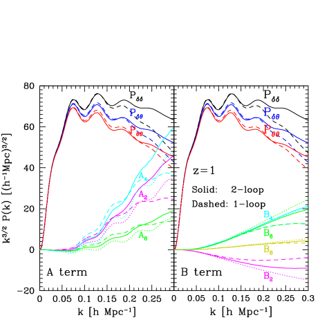
Figure 1: Contribution of the correction terms for the PT model of redshift-space power spectrum. Left and right panels respectively show the $A$ and $B$ terms at $z=1$, respectively. For illustrative purpose, all the results are multiplied by $k^{3/2}$. The $A$ and $B$ terms are expanded as $A(k,\mu)=\sum_{n}^{3}\mu^{2n}\,A_{2n}(k)$ and $B(k,\mu)=\sum_{n}^{4}\mu^{2n}\,B_{2n}(k)$. Here, we plot the scale-dependent coefficients $A_{2n}$ and $B_{2n}$ ($A_{2},\,\,B_{2}$: magenta, $A_{4},\,\,B_{4}$: cyan, $A_{6}\,\,B_{6}$: green, $B_{8}$: yellow). In each panel, solid lines are the corrections for the two-loop contributions, while the dashed lines are the results for the one-loop contributions. For references, the power spectra $P_{\delta\delta}$, $P_{\delta\theta}$, and $P_{\theta\theta}$ computed from RegPT are also shown in black, blue and red lines, respectively.

IV.2 Power spectrum

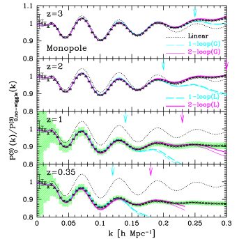
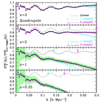
Figure 2: Ratio of power spectra to the smoothed reference spectra in redshift space, $P_{\ell}^{\rm(S)}(k)/P_{\ell,{\rm no\mbox{-}wiggle}}^{\rm(S)}(k)$. Left, middle, and right panels respectively show the monopole ($\ell=0$), quadrupole ($\ell=2$) and hexadecapole ($\ell=4$) contributions to the redshift-space power spectrum. N-body results are taken from the wmap5 simulations of Ref. Taruya et al. (2012). The reference spectrum $P_{\ell,{\rm no\mbox{-}wiggle}}^{\rm(S)}$ is computed with the no-wiggle approximation of the linear transfer function Eisenstein and Hu (1998), taking account of the linear theory of the Kaiser effect. Long-dashed and solid lines respectively indicate the results based on the RegPT calculations at one- and two-loop orders, adopting the Gaussian (thin) and Lorentzian (thick) form of the damping functions. Triangles and squares in middle and right panels are also obtained from the same calculation at one- and two-loop orders, but taking account of the effect of finite grid-size for the power spectrum measurement in $N$-body simulations (see text and Appendix B in detail). For comparison, the $1$-$\sigma$ statistical errors of the hypothetical survey with volumes $V=5\,h^{-3}$ Gpc³ and number density $n=5\times 10^{-4}\,h^{3}$ Mpc^-3 are estimated from Eq. (46), and are depicted as green shaded regions around the N-body results at $z=0.35$ and $1$.

Before presenting a quantitative comparison, we first look at the contribution of each term appeared in the model of RSD. In Fig. 1, for specific redshift $z=1$, we plot the results for $A$ and $B$ terms as well as the power spectra $P_{\delta\delta}$, $P_{\delta\theta}$, and $P_{\theta\theta}$. From the expressions given in Eqs. (40) and (41), the $A$ and $B$ term can be expanded as $A(k,\mu)=\sum_{n}^{3}A_{2n}(k)\mu^{2n}$ and $B(k,\mu)=\sum_{n}^{4}B_{2n}(k)\mu^{2n}$, and we here plot the scale-dependent coefficients $A_{2n}$ and $B_{2n}$ multiplied by $k^{3/2}$ ($A_{2},\,\,B_{2}$: magenta, $A_{4},\,\,B_{4}$: cyan, $A_{6},\,\,B_{6}$: green, $B_{8}$: yellow). Dashed and solid lines respectively indicate the one- and two-loop contributions to the redshift-space power spectrum. For reference, we also plot the results with standard PT calculations in dotted lines. Compared to the standard PT results, the coefficients of the $A$ term are slightly enhanced at the two-loop order, and the oscillatory feature originating from the BAOs is somewhat smeared. This is similar to what we saw in the real-space power spectrum. Fig. 1 apparently indicates that at the two-loop order, the $A$ term seem to eventually dominate the total power spectrum at small scales. However, this is actually not true. Because of the exponential cutoff generically appeared in the multi-point propagators, the amplitudes of both the $A$ and $B$ terms are suppressed at small scales, as similarly seen in the power spectra of the density and velocity fields. This regularized UV property enables us to give a convergent result for the correlation function, although, as a trade-off, the prediction of redshift-space power spectrum eventually becomes inappropriate at some small scales.

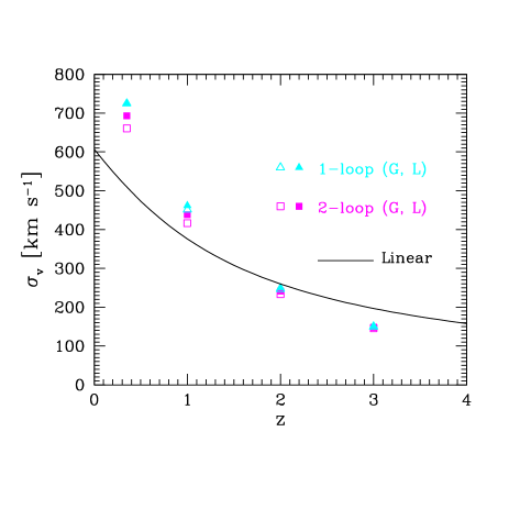
Figure 3: Fitted values of $\sigma_{\rm v}$ as function redshift. Triangles and squares are respectively obtained by fitting the one- and two-loop PT predictions of the monopole and quadrupole spectra to those obtained from the $N$-body simulations. Open (filled) symbols are the fitting results adopting the Gaussian (Lorentzian) form of the damping function in the theoretical predicitons [see Eq. (45)]. For reference, we also plot the linear theory prediction in solid line.

Now, let us compare the predictions of redshift-space power spectrum with those of the $N$-body simulations in greater detail, and investigate the extent to which the PT model reproduces the simulation results. Fig. 2 plots the ratio of power spectra to the smooth reference spectra, $P_{\ell}^{\rm(S)}(k)/P^{\rm(S)}_{\ell,{\rm no\mbox{-}wiggle}}(k)$, where $P^{\rm(S)}_{\ell,{\rm no\mbox{-}wiggle}}(k)$ is the linear power spectrum computed with the no-wiggle formula of Ref. Eisenstein and Hu (1998). The power spectrum $P^{\rm(S)}_{\ell}$ is the $\ell$-th order moment of the redshift-space power spectrum defined by

$$P_{\ell}^{\rm(S)}(k)=\frac{2\ell+1}{2}\,\int_{-1}^{1}d\mu\,P^{\rm(S)}(k,\mu)\,\mathcal{P}_{\ell}(\mu),$$ (42)

with $\mathcal{P}_{\ell}$ being the Legendre polynomials. In Fig. 2, the results of the monopole ($\ell=0$), quadrupole ($\ell=2$), and hexadecapole ($\ell=4$) power spectra are respectively shown from left to right panels. Here, the dashed and solid lines are the results based on the RegPT calculations at the one- and two-loop orders. In plotting these predictions, the velocity dispersion $\sigma_{\rm v}$ in Eq. (8) is treated as a free parameter, and is determined by fitting the model prediction to the $N$-body results of monopole and quadrupole spectra, assuming the Gaussian (thin) and Lorentzian (thick) forms of the damping function $D_{\rm FoG}$:

$$D_{\rm FoG}(x)=\left\{\begin{array}[]{ccl}e^{-x^{2}}&;&\mbox{Gaussian}\\ 1/(1+x^{2}/2)^{2}&;&\mbox{Lorentzian}\end{array}\right.$$ (45)

The predictions were fitted to the simulation results up to the scale indicated by the vertical arrows. Note that this roughly corresponds to the critical wavenumber $k_{\rm crit}$, below which the RegPT prediction in real space agrees with $N$-body simulation at a percent-level precision Taruya et al. (2012). The fitted values of $\sigma_{\rm v}$ are summarized in Fig. 3.

Overall, the agreement between predictions and simulations is remarkably good for the monopole and quadrupole spectra. In both one- and two-loop results, the range of agreement is almost comparable to what we found in the real-space comparison. This is true irrespective of the choice of the damping function. In particular, the two-loop results look very similar to what we obtained with the closure Taruya and Hiramatsu (2008); Taruya et al. (2009) and standard PT calculations Taruya et al. (2010). Rather, with the RegPT, the oscillatory feature in $A$ term is erased, and the contribution of the $A$ term to the BAO structure is somewhat reduced. As a result, the total sum of each contribution closely matches the $N$-body results better than the previous results.

Turning to the hexadecapole power spectra, on the other hand, the simulation results show somewhat noisy behaviors, and it is bit difficult to compare those with the predictions depicted as continuous lines. This noisy structure basically comes from the fact that the power spectra are measured from the grid-assigned density field. Because of the oscillatory feature of the Legendre polynomials $\mathcal{P}_{\ell}$, the measurement of the higher-multipole spectra tends to be sensitively affected by the finite grid-size. In order to remedy this, we also take account of the effect of finite grid-size in the PT prediction, and compute the hexadecapole spectra in the same way as we did in the $N$-body simulations. The detailed prescription of this treatment is presented in Appendix B.

The predictions taking account of the finite-grid size effect are depicted as the triangles and squares for one- and two-loop calculations, respectively. At high-$z$, the PT results faithfully reproduces the noisy behavior in the simulation results. In particular, at low-$k$, the symbols almost overlap each other, indicating that the simulations consistently recover the linear theory prediction. At lower redshifts, on the other hand, there appear small but non-negligible discrepancies. To see the significance of this, we consider the hypothetical galaxy survey, and estimate the expected $1$-$\sigma$ statistical errors, $\Delta P_{\ell}^{\rm(S)}$, depicted as green shaded region at $z=0.35$ and $1$ in Fig. 2. The statistical error $\Delta P_{\ell}^{\rm(S)}$ is simply computed with

$$[\Delta P_{\ell}^{\rm(S)}(k)]^{2}=\frac{2}{N_{k}}\,\sigma_{P,\ell}^{2}(k)\,\,;\quad N_{k}=\frac{4\pi\,k^{2}\Delta k}{(2\pi/V^{1/3})^{3}},$$ (46)

with the function $\sigma_{P,\ell}$ given by

$$\sigma_{P,\ell}^{2}(k)=\frac{(2\ell+1)^{2}}{2}\int_{-1}^{1}d\mu\left\{P^{\rm(S)}_{\rm lin}(k,\mu)+\frac{1}{n}\right\}^{2},$$ (47)

where $P^{\rm(S)}_{\rm lin}$ is the linear power spectrum, and the $\Delta k$ is the bin width for which we adopt the same bin size used in the $N$-body data. The volume and the number density of the hypothetical survey are respectively set to $V=5\,h^{-3}$ Gpc³ and $n=5\times 10^{-4}\,h^{3}$  Mpc^-3, which roughly correspond to those of the Baryon Oscillation Spectroscopic Survey (BOSS) or the survey with Subaru Measurement of Images and Redshifts (SuMIRe) with Prime Focus Spectrograph (PFS) . Then, we found that the predicted monopole and quadrupole spectra agree with simulations well within the statistical error, while the discrepancy in the hexadecapole spectra is marginal or even exceeds the $1$-$\sigma$ error at high-$k$, depending on the functional form of the damping function $D_{\rm FoG}$. These results not only indicate the sensitive dependence of the damping function but also suggest a possible deficit in the RSD model when predicting the higher-multipole spectra. This point will be further discussed in greater detail in Sec. V.

IV.3 Correlation function

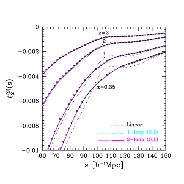
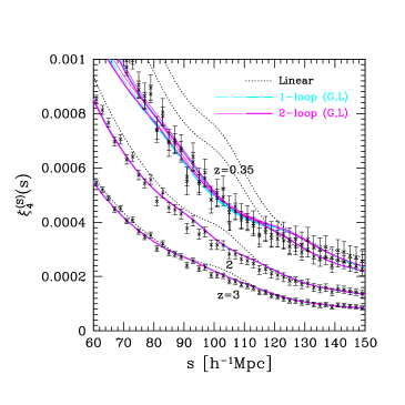
Figure 4: Redshift-space correlation functions around the baryon acoustic peak. Monopole ($\ell=0$), quadrupole ($\ell=2$), and hexadecapole ($\ell=4$) moments of the redshift-space correlation function are respectively shown in left, middle and right panels. Dotted lines are the linear theory predictions, while the dashed and solid lines respectively represent the results based on the RSD model using the RegPT up to the one- and two-loop orders, adopting the Gaussian (thin) and Lorentzian (thick) damping function.

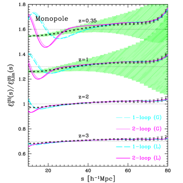
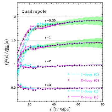
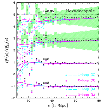
Figure 5: Redshift-space correlation functions at small scales. Plotted results are the ratio of correlation function to the linear theory predictions taking account of the linear Kaiser factor, i.e., $\xi_{\ell}^{\rm(S)}(s)/\xi_{\ell,{\rm lin}}^{\rm(S)}(s)$. For clarity, we artificially shift the results at each redshift by a constant value (indicated by the horizontal dotted line). Symbols and line types are the same as those in Fig. 2. The green shaded regions at $z=0.35$ and $1$ indicate the expected $1$-$\sigma$ error of the hypothetical galaxy survey with the volume $V=5\,h^{-3}$ Gpc³ and number density $n=5\times 10^{-4}\,h^{3}$ Mpc^-3.

We next consider the correlation function. We first show in Fig. 4 the the large-scale behavior of the correlation functions, focusing on scales around the baryon acoustic peak. Left, middle and right panels respectively plot the results of monopole, quadrupole, and hexadecapole correlation functions. The predictions depicted as solid and dashed lines are basically obtained from the power spectra through the relation:

$$\xi_{\ell}^{\rm(S)}(s)=i^{\ell}\int\frac{dk\,k^{2}}{2\pi^{2}}\,P_{\ell}^{\rm(S)}(k)\,j_{\ell}(ks).$$ (48)

Note again that thin and thick lines represent the predictions adopting the Gaussian and Lorentzian damping functions, and we use the same velocity dispersion $\sigma_{\rm v}$ as determined in the power spectrum analysis. At all redshifts, the one- and two-loop results do indeed agree with $N$-body results quite well. This is to be contrasted with previous studies neglecting $A$ and $B$ terms Taruya et al. (2009), in which the power spectra, $P_{\delta\delta}$, $P_{\delta\theta}$ and $P_{\theta\theta}$, are computed with closure theory. Now with the coherent treatment with RegPT, the model successfully describes the correlation functions around the baryon acoustic peak. The results show that at large-scales, the choice of the damping function hardly change the prediction, and both the one- and two-loop predictions almost coincide each other.

Let us look at the small-scale behaviors beyond the baryon acoustic scales. Fig. 5 shows the ratio of the correlation functions to the linear theory predictions, $\xi^{\rm(S)}_{\ell}(s)/\xi^{\rm(S)}_{\ell,{\rm lin}}(s)$, specifically focusing on the scales $10\,h^{-1}$ Mpc $\leq s\leq$ $80\,h^{-1}$ Mpc. Note that the linear theory prediction $\xi^{\rm(S)}_{\ell,{\rm lin}}$ is made with the linear power spectrum taking only account of the linear Kaiser effect. As references, we also consider the hypothetical galaxy survey, and show the $1$-$\sigma$ statistical errors at $z=0.35$ and $1$, depicted as green shaded region. This is estimated from

$$[\Delta\xi_{\ell}^{\rm(S)}(s)]^{2}=\frac{2}{V}\int\frac{dk\,k^{2}}{2\pi^{2}}\left\{j_{\ell}(k\,s)\,\sigma_{P,\ell}(k)\right\}^{2}$$ (49)

with $\sigma_{P,\ell}$ defined in Eq. (47). Here, we adopt the same survey parameters as we considered in Fig. 2.

As anticipated from the power spectrum results, the predictions for both the monopole and quadrupole moments perfectly agree well with simulations at the scales, $s\gtrsim 10-30\,h^{-1}$ Mpc, depending on the redshift. The range of agreement with $N$-body simulations is comparable to the one obtained in real space, and roughly matches the range inferred from the power spectrum results. One noticeable point in the prediction of correlation function is that even the one-loop results do give an accurate prediction over a wide range of correlation function, where the choice of damping function hardly change the results.

On the other hand, similar to the power spectrum analysis, the measured hexadecapole moment suffers from the effect of finite grid-size, and in order to make a fair comparison, we need to incorporate the effect of this into the theoretical calculation. The triangles and squares are the results taking account of the finite grid-size based on the prescription in Appendix B. Then, the predictions at high-$z$ reproduce the $N$-body results almost perfectly, while we find a systematic discrepancy at low-$z$, where the results also show a sensitive dependence on the choice of the damping function. However, we note that the discrepancy seen in the correlation function is smaller than the statistical errors of the hypothetical surveys, and it seems less significant compared to the results in power spectrum. This is partly because many Fourier modes can contribute to the correlation function, and they help to mitigate the significance of the discrepancy seen in the power spectrum at some specific modes. Strictly speaking, the amplitudes of the correlation function are strongly correlated between different scales, and the error covariance of the correlation function may be important to rigorously judge the significance of the discrepancy. Rather, a conservative and generic statement is that for the scales where both the one- and two-loop predictions coincide each other, the non-linear effect of RSD and gravity can be small, and thus the discrepancy between the PT predictions and simulations is insignificant.

V Impact of higher-order corrections

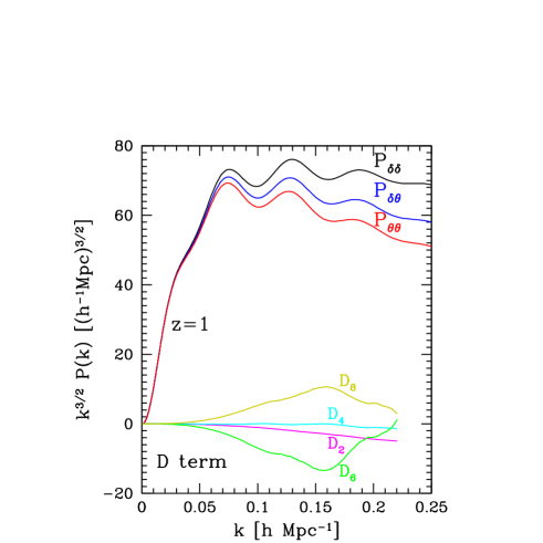
Figure 6: Same as in Fig. 1, but the scale-dependent coefficient of the $D$ term at $z=1$ is plotted ($D_{2}$: magenta, $D_{4}$: cyan, $D_{6}$: green, $D_{8}$: yellow). For reference, the power spectra $P_{\delta\delta}$, $P_{\delta\theta}$, and $P_{\theta\theta}$ computed from the RegPT at two-loop order are also shown.

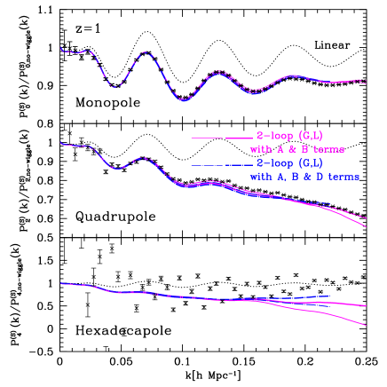
So far, we have neglected the contribution of the $D$ term [Eq. (12)] to the predictions of redshift-space power spectrum. Strictly speaking, this is no longer valid when we perform the two-loop calculations. The higher-order corrections of the RSD such as the $D$ term may help us to explain the small discrepancy seen in the hexadecapole power spectrum. In this section, we quantitatively compute the $D$ term, and discuss the validity of the analysis in previous section. Further, using the measured power spectrum of the $N$-body simulation, we also estimate the magnitude of a possible systematics coming from the higher-order corrections to the RSD.

Let us first consider the $D$ term. Eq. (12) can be recast as

$$D(k,\mu)=(k\mu\,f)^{2}\int\frac{d^{3}\mbox{\boldmath$p$}d^{3}\mbox{\boldmath$q$}}{(2\pi)^{6}}\,\frac{p_{z}q_{z}}{(pq)^{2}}$$

$$\quad\times\left\{T_{\sigma}(\mbox{\boldmath$p$},\mbox{\boldmath$q$},-\mbox{\boldmath$k$}-\mbox{\boldmath$p$}-\mbox{\boldmath$q$},\mbox{\boldmath$k$})-T_{\sigma}(\mbox{\boldmath$p$},\mbox{\boldmath$q$},\mbox{\boldmath$k$}-\mbox{\boldmath$p$},-\mbox{\boldmath$k$}-\mbox{\boldmath$q$})\right\},$$ (50)

where the function $T_{\sigma}$ is the cross trispectrum defined by

$$\left\langle\theta(\mbox{\boldmath$k$}_{1})\langle\theta(\mbox{\boldmath$k$}_{2})\left\{\delta(\mbox{\boldmath$k$}_{3})+f\,\frac{k_{3z}^{2}}{k_{3}^{2}}\theta(\mbox{\boldmath$k$}_{3})\right\}\left\{\delta(\mbox{\boldmath$k$}_{4})+f\,\frac{k_{4z}^{2}}{k_{4}^{2}}\theta(\mbox{\boldmath$k$}_{4})\right\}\right\rangle_{c}$$

$$\quad=(2\pi)^{3}\delta_{D}(\mbox{\boldmath$k$}_{1}+\mbox{\boldmath$k$}_{2}+\mbox{\boldmath$k$}_{3}+\mbox{\boldmath$k$}_{4})\,T_{\sigma}(\mbox{\boldmath$k$}_{1},\mbox{\boldmath$k$}_{2},\mbox{\boldmath$k$}_{3},\mbox{\boldmath$k$}_{4}).$$ (51)

In deriving the above expression, we have used the symmetric properties of the trispectrum $T_{\sigma}$, i.e., $T_{\sigma}(\mbox{\boldmath$k$}_{1},\mbox{\boldmath$k$}_{2},\mbox{\boldmath$k$}_{3},\mbox{\boldmath$k$}_{4})=T_{\sigma}(-\mbox{\boldmath$k$}_{1},-\mbox{\boldmath$k$}_{2},-\mbox{\boldmath$k$}_{3},-\mbox{\boldmath$k$}_{4})=T_{\sigma}(\mbox{\boldmath$k$}_{2},\mbox{\boldmath$k$}_{1},\mbox{\boldmath$k$}_{3},\mbox{\boldmath$k$}_{4})=T_{\sigma}(\mbox{\boldmath$k$}_{1},\mbox{\boldmath$k$}_{2},\mbox{\boldmath$k$}_{4},\mbox{\boldmath$k$}_{3})$. The trispectrum $T_{\sigma}$ is rewritten with the sum of the cross power spectrum $T_{abcd}$ for the doublet $\Psi_{a}$ as

$$T_{\sigma}(\mbox{\boldmath$k$}_{1},\mbox{\boldmath$k$}_{2},\mbox{\boldmath$k$}_{3},\mbox{\boldmath$k$}_{4})=T_{2211}(\mbox{\boldmath$k$}_{1},\mbox{\boldmath$k$}_{2},\mbox{\boldmath$k$}_{3},\mbox{\boldmath$k$}_{4})$$

$$\qquad\qquad\qquad+f\,\left(\frac{k_{3,z}}{k_{3}}\right)^{2}\,T_{2221}(\mbox{\boldmath$k$}_{1},\mbox{\boldmath$k$}_{2},\mbox{\boldmath$k$}_{3},\mbox{\boldmath$k$}_{4})$$

$$\qquad\qquad\qquad+f\,\left(\frac{k_{4,z}}{k_{4}}\right)^{2}\,T_{2212}(\mbox{\boldmath$k$}_{1},\mbox{\boldmath$k$}_{2},\mbox{\boldmath$k$}_{3},\mbox{\boldmath$k$}_{4})$$

$$\qquad\qquad\qquad+f^{2}\,\left(\frac{k_{3,z}k_{4,z}}{k_{3}k_{4}}\right)^{2}\,T_{2222}(\mbox{\boldmath$k$}_{1},\mbox{\boldmath$k$}_{2},\mbox{\boldmath$k$}_{3},\mbox{\boldmath$k$}_{4}),$$ (52)

which can be computed with RegPT. For the predictions of redshift-space power spectrum at two-loop order, it is sufficient to give the tree-level results for $T_{abcd}$, whose explicit expression is given in Appendix A.3.

Fig. 6 shows the $D$ term computed at specific redshift $z=1$. Similar to the $A$ and $B$ terms, the $D$ term can be expanded in powers of $\mu$ [see Eqs. (50) and (52)]: $D(k,\mu)=\sum_{n=1}^{4}\,\mu^{2n}\,D_{2n}(k)$. We then plot the coefficients $D_{2n}$ as function of wavenumber. Note that unlike the $A$ and $B$ terms, we were not able to derive a simpler expression like Eqs. (40) and (41). Hence, we employed the Monte Carlo technique to directly perform the six-dimensional integral in Eqs. (50), and obtained the result in $(k,\mu)$-plane. For each wavenumber, we applied the multipole expansion, and characterize the $\mu$-dependence of the $D$ term by the Legendre polynomials. Finally, the resultant coefficients are translated into those in the power-law expansion, $D_{2n}$.

Figure 7: Ratio of power spectra to the smoothed reference spectra in redshift space, $P_{\ell}^{\rm(S)}(k)/P_{\ell,{\rm no\mbox{-}wiggle}}^{\rm(S)}(k)$ for the predictions including the $D$ terms (blue dot-dashed). The results at $z=1$ are specifically shown. For comparison, the two-loop results ignoring the $D$ terms are also shown (magenta solid). Thin and thick lines are the results adopting the Gaussian and Lorentzian damping function, respectively.

The $D$ term shown in Fig. 6 has the amplitudes roughly comparable to the $B$ term. However, a careful look at the $\mu$-dependence reveals that the coefficients $D_{2}$ and $D_{4}$ are rather small. Also, while the amplitude is non-negligible for $D_{6}$ and $D_{8}$, their signs are opposite each other. These facts imply that when convolving with the damping function $D_{\rm FoG}$, the contribution of the $D$ term becomes negligible for the monopole and quadrupole spectra, and is largely canceled for the hexadecapole power spectrum. This is indeed manifested in Fig. 7, where we compare the model prediction including the $D$ term (blue dot-dashed) with $N$-body simulations. Except for a slight change in the hexadecapole, which makes the prediction slightly better if we adopt the Lorentzian damping function, the resultant power spectra are hardly affected by the $D$ term. The fitted value of the parameter $\sigma_{\rm v}$ almost remains the same. Therefore, we conclude that the actual contribution of the $D$ term is less significant for the prediction of redshift-space power spectrum.

Figure 8: The ratio of power spectra measured in $(k,\mu)$ space from the simulations to those from the theoretical calculation [see Eq.(53)]. The results at $z=1$ are plotted as function of $k\mu$. The color scale indicate the power spectrum contribution at different range of wavenumbers. Left panel shows the results ignoring all the corrections, $A$, $B$ and $D$ terms, in the theoretical calculation. The middle and right panels are the results taking account of the corrections, but in middle panel, the $D$ term is neglected. For reference, we also show the Gaussian ($D_{\rm FoG}=\exp\{-(k\,\mu\,f\,\sigma_{\rm v})^{2}\}$, solid) and Lorentzian ($D_{\rm FoG}=1/\{1+(k\,\mu\,f\,\sigma_{\rm v})^{2}/2\}^{2}$, dashed) damping functions adopting the fitted values of $\sigma_{\rm v}$.

Nevertheless, this does not prove that the corrections higher than the $D$ term originated from the low-$k$ expansion in Eq. (7) are entirely negligible. Further, as we saw in previous section, there appears a small but non-negligible difference in the hexadecapole spectrum between the model predictions and $N$-body simulations (Fig. 2). Since a part of our RSD model has not been derived by the perturbative expansion, there would exist some missing corrections that can systematically affect the prediction of higher-multipole power spectra.

In order to elucidate the potential systematics, we measure the power spectrum of $N$-body simulations in $(k,\mu)$ space, and divide it by the PT prediction in the following way:

$$\frac{P_{\rm N\mbox{-}body}^{\rm(S)}(k,\mu)}{P_{\rm Kaiser}(k,\mu)+A(k,\mu)+B(k,\mu)+D(k,\mu)}$$ (53)

In Fig. 8, the results at $z=1$ are plotted as the function of the single variable, $k\mu$. The color scales represent the contributions from the different wavenumbers. The plotted results are the residual contributions of the RSD that is not described by the low-$k$ expansion, but is rather characterized by the damping function $D_{\rm FoG}$ in our PT model [Eq. (8)]. Compared to the case ignoring the correction terms (left panel), the residuals shown in the middle and right panels are mostly characterized by the single-valued function of $k\mu$, and within the plotted range, they are approximately described by the Gaussian ($D_{\rm FoG}=e^{-(k\mu f\sigma_{\rm v})^{2}}$, solid lines) or Lorentzian ($D_{\rm FoG}=1/\{1+(k\mu f\sigma_{\rm v})^{2}/2\}^{2}$, dashed lines) damping function. This is indeed what we expected from our RSD model.

However, a closer look at the scatter around the damping functions reveals some systematics that the low-$k$ residuals tend to take larger values, while the high-$k$ residuals take slightly smaller values than the Gaussian or Lorentzian damping function, indicating the imperfect modeling of RSD. These systematics in the scatter would be certainly the source of the discrepancy seen in the hexadecapole power spectrum. In this respect, a better description for the power spectrum suppression might be crucial for an accurate prediction of higher-multipole spectra. Recent study by Ref. Vlah et al. (2012) suggests that a simple prescription with the function $D_{\rm FoG}$ might be a oversimplified treatment, and the suppression of power spectrum cannot be controlled by a single parameter $\sigma_{\rm v}$. These two facts may pose a caution for the assumption of our model, and the suppression and modulation of the power spectrum might not be treated separately. Thus, in general, a more elaborate modeling of RSD is needed for an accurate prediction of higher multipole power spectra, although the actual impact of such a modeling on the cosmological application is unclear, and is beyond the scope of this paper.

VI Conclusion

In this paper, we have implemented the resummed PT scheme called RegPT, which based on a multi-point propagator expansion, together with an improved model of redshift-space distortions (RSD), in order to compute the matter two-point statistical properties in redshift space, both in Fourier and in configuration spaces. For the first time, calculations consistently include PT corrections up to the two-loop order. Our analytical predictions are then compared with $N$-body simulations. We found that, whenever predictions are at percent level in real space, a similar performance can be obtained in redshift space. With a full implementation of the RegPT scheme, the present work puts forward proper PT calculations in redshift space, allowing the predictions to be greatly improved in the sense that we are now able to give a consistent prediction not only for the power spectrum but also for the correlation function. This is in marked contrast to the previous analysis partly using the standard PT treatment.

We have also investigated the influence of higher-order corrections in redshift space. While our RSD model has been derived based on the low-$k$ expansion, the previous studies have missed the non-Gaussian correction at the trispectrum order called $D$ term, whose contribution is comparable to the two-loop order. We have computed the $D$ term explicitly, and confirmed that the amplitude of the coefficients given in powers of $\mu$ are comparable to that of the $B$ term. The actual contribution to the power spectrum, however, turns out to be small and it would only affect the higher-multipole spectra. Nevertheless, the present RSD model seems to have a slight deficit in the prediction of the higher multipoles, and we have quantified the validity of our model assumption with a help of $N$-body simulations. The results in Fig. 8 indicate an improper treatment for the damping effect of the power spectrum, and this would lead to the small discrepancy of the higher multipoles between predictions and simulations.

Nevertheless, the actual impact of the improper modeling of RSD might be less significant, considering the other big systematics such as the galaxy bias. Indeed, one crucial aspect of the galaxy bias in redshift space is that it can affect both the density and velocity fields, and the clustering feature in redshift space cannot be straightforwardly understood from the real-space clustering. We have previously shown that our model of RSD, combined with the simple linear bias, can successfully describe the redshift-space halo clustering in $N$-body simulations quite well. Still, however, this should be regarded as an idealistic example. In reality, galaxies do not faithfully trace the halo clustering, and peculiar velocity of galaxies certainly differs from the center-of-mass velocity of halos. As it has been recently advocated in Ref. Hikage et al. (2012a), off-centered galaxies can have a large peculiar velocity due to the virial motion, and the presence of these galaxies can drastically change the power spectrum Hikage et al. (2012b); Masaki et al. (2012). The significance of this effect may sensitively depend on the type of the targeted galaxies. A careful study of the galaxy samples is quite crucial for the cosmological analysis to get an unbiased cosmological constraint.

Appendix A Explicit expressions for regularized power spectrum, bispectrum and trispectrum

In this Appenix, based on the regularized $\Gamma$ expansion, we give full expressions for the real-space power spectra and bispectra used to compute the redshift-space power spectrum and correlation function.

A.1 Power spectrum

According to the prescription described in Sec. III, the power spectrum at one-loop order of the $\Gamma$-expansion becomes

$$P_{ab}(k;\eta)=\Gamma_{a,{\rm reg}}^{(1)}(k;\eta)\Gamma_{b,{\rm reg}}^{(1)}(k;\eta)P_{0}(k)+2\int\frac{d^{3}\mbox{\boldmath$q$}}{(2\pi)^{3}}\,\Gamma_{a,{\rm reg}}^{(2)}(\mbox{\boldmath$q$},\mbox{\boldmath$k$}-\mbox{\boldmath$q$};\eta)\Gamma_{b,{\rm reg}}^{(2)}(\mbox{\boldmath$q$},\mbox{\boldmath$k$}-\mbox{\boldmath$q$};\eta)P_{0}(q)P_{0}(|\mbox{\boldmath$k$}-\mbox{\boldmath$q$}|)$$ (54)

with the regularized propagators $\Gamma^{(1)}_{\rm reg}$ and $\Gamma^{(2)}_{\rm reg}$ valid at one-loop order being:

$$\Gamma_{a,{\rm reg}}^{(1)}(k;\eta)=e^{\eta}\left[1+\frac{k^{2}\sigma_{\rm v}^{2}e^{2\eta}}{2}+e^{2\eta}\,\overline{\Gamma}^{(1)}_{a,{\rm 1\mbox{-}loop}}(k)\right]\exp\left\{-\frac{k^{2}\sigma_{\rm v}^{2}e^{2\eta}}{2}\right\},$$ (55)

$$\Gamma_{a,{\rm reg}}^{(2)}(\mbox{\boldmath$q$},\mbox{\boldmath$k$}-\mbox{\boldmath$q$};\eta)=e^{2\eta}F_{a}^{(2)}(\mbox{\boldmath$q$},\mbox{\boldmath$k$}-\mbox{\boldmath$q$})\,\exp\left\{-\frac{k^{2}\sigma_{\rm v}^{2}e^{2\eta}}{2}\right\}.$$ (56)

On the other hand, if we include the next-to-leading order contribution, i.e., two-loop corrections, the resultant expression becomes

$$P_{ab}(k;\eta)=\Gamma_{a,{\rm reg}}^{(1)}(k;\eta)\Gamma_{b,{\rm reg}}^{(1)}(k;\eta)P_{0}(k)+2\int\frac{d^{3}\mbox{\boldmath$q$}}{(2\pi)^{3}}\,\Gamma_{a,{\rm reg}}^{(2)}(\mbox{\boldmath$q$},\mbox{\boldmath$k$}-\mbox{\boldmath$q$};\eta)\Gamma_{b,{\rm reg}}^{(2)}(\mbox{\boldmath$q$},\mbox{\boldmath$k$}-\mbox{\boldmath$q$};\eta)P_{0}(q)P_{0}(|\mbox{\boldmath$k$}-\mbox{\boldmath$q$}|)$$

$$\qquad\qquad\qquad\qquad+6\int\frac{d^{6}\mbox{\boldmath$p$}d^{3}\mbox{\boldmath$q$}}{(2\pi)^{6}}\,\Gamma_{a,{\rm reg}}^{(3)}(\mbox{\boldmath$p$},\mbox{\boldmath$q$},\mbox{\boldmath$k$}-\mbox{\boldmath$p$}-\mbox{\boldmath$q$};\eta)\Gamma_{b,{\rm reg}}^{(3)}(\mbox{\boldmath$p$},\mbox{\boldmath$q$},\mbox{\boldmath$k$}-\mbox{\boldmath$p$}-\mbox{\boldmath$q$};\eta)P_{0}(p)P_{0}(q)P_{0}(|\mbox{\boldmath$k$}-\mbox{\boldmath$p$}-\mbox{\boldmath$q$}|)$$ (57)

with the regularized propagators given by

$$\Gamma_{a,{\rm reg}}^{(1)}(k;\eta)=e^{\eta}\left[1+\frac{k^{2}\sigma_{\rm v}^{2}e^{2\eta}}{2}+\frac{1}{2}\left(\frac{k^{2}\sigma_{\rm v}^{2}e^{2\eta}}{2}\right)^{2}+e^{2\eta}\,\overline{\Gamma}^{(1)}_{a,{\rm 1\mbox{-}loop}}(k)\left\{1+\frac{k^{2}\sigma_{\rm v}^{2}e^{2\eta}}{2}\right\}+e^{4\eta}\,\overline{\Gamma}^{(1)}_{a,{\rm 2\mbox{-}loop}}(k)\right]\exp\left\{-\frac{k^{2}\sigma_{\rm v}^{2}e^{2\eta}}{2}\right\},$$ (58)

$$\Gamma_{a,{\rm reg}}^{(2)}(\mbox{\boldmath$q$},\mbox{\boldmath$k$}-\mbox{\boldmath$q$};\eta)=e^{2\eta}\left[F_{a}^{(2)}(\mbox{\boldmath$q$},\mbox{\boldmath$k$}-\mbox{\boldmath$q$})\left\{1+\frac{k^{2}\sigma_{\rm v}^{2}e^{2\eta}}{2}\right\}+e^{2\eta}\,\overline{\Gamma}^{(2)}_{a,{\rm 1\mbox{-}loop}}(\mbox{\boldmath$q$},\mbox{\boldmath$k$}-\mbox{\boldmath$q$})\right]\exp\left\{-\frac{k^{2}\sigma_{\rm v}^{2}e^{2\eta}}{2}\right\},$$ (59)

$$\Gamma_{a,{\rm reg}}^{(3)}(\mbox{\boldmath$p$},\mbox{\boldmath$q$},\mbox{\boldmath$k$}-\mbox{\boldmath$p$}-\mbox{\boldmath$q$};\eta)=e^{3\eta}\,F_{a}^{(3)}(\mbox{\boldmath$p$},\mbox{\boldmath$q$},\mbox{\boldmath$k$}-\mbox{\boldmath$p$}-\mbox{\boldmath$q$})\exp\left\{-\frac{k^{2}\sigma_{\rm v}^{2}e^{2\eta}}{2}\right\},$$ (60)

where the quantity $\overline{\Gamma}_{p\mbox{-}{\rm loop}}^{(n)}$ is defined in Eq. (32). The higher-order contributions up to the two- and one-loop order of the propagators are respectively included in the expression of the regularized propagators $\Gamma_{a,{\rm reg}}^{(1)}$ and $\Gamma_{a,{\rm reg}}^{(2)}$, consistently with the $\Gamma$-expansion at two-loop order. The detailed prescription on how to efficiently compute each contribution is described in Ref. Taruya et al. (2012). Shortly, we use the analytic expression of the kernels to compute $\overline{\Gamma}_{p\mbox{-}{\rm loop}}^{(n)}$ ($\overline{\Gamma}_{1\mbox{-}{\rm loop}}^{(2)}$ for Bernardeau et al. (2012b) and $\overline{\Gamma}_{2\mbox{-}{\rm loop}}^{(1)}$ for Bernardeau et al. (2012c)), and the integrals are performed with the method of Gaussian quadrature. For the integral in the last term of Eq. (54), we adopt the Monte Carlo technique using the publicly available library called CUBA Hahn (2005).

A.2 Bispectrum

The real-space bispectra are needed to compute the $A$ term, and for a consistent calculation of the redshift-space power spectrum up to two-loop order, we need the bispectra at one-loop order. In this case, we can decomposed the bispectrum into three pieces:

$$B_{abc}(\mbox{\boldmath$k$}_{1},\mbox{\boldmath$k$}_{2},\mbox{\boldmath$k$}_{3})=B_{abc}^{I}(\mbox{\boldmath$k$}_{1},\mbox{\boldmath$k$}_{2},\mbox{\boldmath$k$}_{3})$$

$$\qquad+B_{abc}^{II}(\mbox{\boldmath$k$}_{1},\mbox{\boldmath$k$}_{2},\mbox{\boldmath$k$}_{3})+B_{abc}^{III}(\mbox{\boldmath$k$}_{1},\mbox{\boldmath$k$}_{2},\mbox{\boldmath$k$}_{3}).$$ (61)

These three contributions are expressed in terms of the multi-point propagator $\Gamma^{(p)}$ Bernardeau et al. (2012b):

$$B_{abc}^{I}(\mbox{\boldmath$k$}_{1},\mbox{\boldmath$k$}_{2},\mbox{\boldmath$k$}_{3})=2\,\left\{\Gamma^{(2)}_{a,{\rm reg}}(\mbox{\boldmath$k$}_{2},\mbox{\boldmath$k$}_{3})\Gamma_{b,{\rm reg}}^{(1)}(k_{2})\Gamma_{c,{\rm reg}}^{(1)}(k_{3})\,P_{0}(k_{2})P_{0}(k_{3})\right.$$

$$\left.\qquad\qquad+\Gamma^{(2)}_{b,{\rm reg}}(\mbox{\boldmath$k$}_{1},\mbox{\boldmath$k$}_{3})\Gamma_{a,{\rm reg}}^{(1)}(k_{1})\Gamma_{c,{\rm reg}}^{(1)}(k_{3})\,P_{0}(k_{1})P_{0}(k_{3})+\Gamma^{(2)}_{c,{\rm reg}}(\mbox{\boldmath$k$}_{1},\mbox{\boldmath$k$}_{2})\Gamma_{a,{\rm reg}}^{(1)}(k_{1})\Gamma_{b,{\rm reg}}^{(1)}(k_{2})\,P_{0}(k_{1})P_{0}(k_{2})\right\},$$ (62)

$$B_{abc}^{II}(\mbox{\boldmath$k$}_{1},\mbox{\boldmath$k$}_{2},\mbox{\boldmath$k$}_{3})=8\,\int\frac{d^{3}\mbox{\boldmath$q$}}{(2\pi)^{3}}\,\Gamma_{a,{\rm reg}}^{(2)}(\mbox{\boldmath$k$}_{1}-\mbox{\boldmath$q$},\mbox{\boldmath$q$})\,\Gamma_{b,{\rm reg}}^{(2)}(\mbox{\boldmath$k$}_{2}+\mbox{\boldmath$q$},-\mbox{\boldmath$q$})\,\Gamma_{c,{\rm reg}}^{(2)}(-\mbox{\boldmath$q$}-\mbox{\boldmath$k$}_{2},-\mbox{\boldmath$k$}_{1}+\mbox{\boldmath$q$})\,$$

$$\qquad\qquad\qquad\qquad\qquad\qquad\times\,P_{0}(|\mbox{\boldmath$k$}_{1}-\mbox{\boldmath$q$}|)P_{0}(|\mbox{\boldmath$k$}_{2}+\mbox{\boldmath$q$}|)P_{0}(q),$$ (63)

$$B_{abc}^{III}(\mbox{\boldmath$k$}_{1},\mbox{\boldmath$k$}_{2},\mbox{\boldmath$k$}_{3})=6\,\int\frac{d^{3}\mbox{\boldmath$q$}}{(2\pi)^{3}}\,\left\{\Gamma_{a,{\rm reg}}^{(3)}(-\mbox{\boldmath$k$}_{3},-\mbox{\boldmath$k$}_{2}+\mbox{\boldmath$q$},-\mbox{\boldmath$q$})\,\Gamma_{b,{\rm reg}}^{(2)}(\mbox{\boldmath$k$}_{2}-\mbox{\boldmath$q$},\mbox{\boldmath$q$})\,\Gamma_{c,{\rm reg}}^{(1)}(k_{3})\,\,P_{0}(|\mbox{\boldmath$k$}_{2}-\mbox{\boldmath$q$}|)P_{0}(q)P_{0}(k_{3})\right.$$

$$\qquad\qquad\qquad\qquad\qquad\qquad~{}+\Gamma_{a,{\rm reg}}^{(3)}(-\mbox{\boldmath$k$}_{2},-\mbox{\boldmath$k$}_{3}+\mbox{\boldmath$q$},-\mbox{\boldmath$q$})\,\Gamma_{b,{\rm reg}}^{(1)}(k_{2})\,\Gamma_{c,{\rm reg}}^{(2)}(\mbox{\boldmath$k$}_{3}-\mbox{\boldmath$q$},\mbox{\boldmath$q$})\,\,P_{0}(|\mbox{\boldmath$k$}_{3}-\mbox{\boldmath$q$}|)P_{0}(q)P_{0}(k_{2})$$

$$\qquad\qquad\qquad\qquad\qquad\qquad~{}+\Gamma_{a,{\rm reg}}^{(2)}(\mbox{\boldmath$k$}_{1}-\mbox{\boldmath$q$},\mbox{\boldmath$q$})\,\Gamma_{b,{\rm reg}}^{(3)}(-\mbox{\boldmath$q$},-\mbox{\boldmath$k$}_{1}+\mbox{\boldmath$q$},-\mbox{\boldmath$k$}_{3})\,\Gamma_{c,{\rm reg}}^{(1)}(k_{3})\,\,P_{0}(|\mbox{\boldmath$k$}_{1}-\mbox{\boldmath$q$}|)P_{0}(q)P_{0}(k_{3})$$

$$\qquad\qquad\qquad\qquad\qquad\qquad~{}+\Gamma_{a,{\rm reg}}^{(1)}(k_{1})\,\Gamma_{b,{\rm reg}}^{(3)}(-\mbox{\boldmath$k$}_{1},-\mbox{\boldmath$k$}_{3}+\mbox{\boldmath$q$},-\mbox{\boldmath$q$})\,\Gamma_{c,{\rm reg}}^{(2)}(\mbox{\boldmath$k$}_{3}-\mbox{\boldmath$q$},\mbox{\boldmath$q$})\,\,P_{0}(k_{1})P_{0}(q)P_{0}(|\mbox{\boldmath$k$}_{3}-\mbox{\boldmath$q$}|)$$

$$\qquad\qquad\qquad\qquad\qquad\qquad~{}+\Gamma_{a,{\rm reg}}^{(2)}(\mbox{\boldmath$k$}_{1}-\mbox{\boldmath$q$},\mbox{\boldmath$q$})\,\Gamma_{b,{\rm reg}}^{(1)}(k_{2})\,\Gamma_{c,{\rm reg}}^{(3)}(-\mbox{\boldmath$k$}_{1}+\mbox{\boldmath$q$},-\mbox{\boldmath$q$},-\mbox{\boldmath$k$}_{2})\,\,P_{0}(|\mbox{\boldmath$k$}_{1}-\mbox{\boldmath$q$}|)P_{0}(q)P_{0}(k_{2})$$

$$\qquad\qquad\qquad\qquad\qquad\qquad~{}\left.+\Gamma_{a,{\rm reg}}^{(1)}(k_{1})\,\Gamma_{b,{\rm reg}}^{(2)}(\mbox{\boldmath$k$}_{2}-\mbox{\boldmath$q$},\mbox{\boldmath$q$})\,\Gamma_{c,{\rm reg}}^{(3)}(-\mbox{\boldmath$k$}_{1},-\mbox{\boldmath$q$},-\mbox{\boldmath$k$}_{2}+\mbox{\boldmath$q$})\,\,P_{0}(k_{1})P_{0}(q)P_{0}(|\mbox{\boldmath$k$}_{2}-\mbox{\boldmath$q$}|).\,\right\}$$ (64)

For the bispectrum $B_{abc}^{I}$, the regularized multipoint propagators valid at one-loop order are computed with Eq. (55) for $\Gamma^{(1)}_{a,{\rm reg}}$ and Eq. (59) for $\Gamma^{(2)}_{a,{\rm reg}}$. On the other hand, for the contributions $B_{abc}^{II}$ and $B_{abc}^{III}$, the tree-level propagator with exponential cutoff is sufficient for a consistent calculation at one-loop order. Explicitly, it is given by

$$\Gamma^{(n)}_{a,{\rm reg}}(\mbox{\boldmath$k$}_{1},\cdots,\,\mbox{\boldmath$k$}_{n})=F_{a}^{(n)}(\mbox{\boldmath$k$}_{1},\cdots,\,\mbox{\boldmath$k$}_{n})\,\exp\left\{-\frac{k^{2}\sigma_{d}^{2}\,e^{2\,\eta}}{2}\right\}$$ (65)

with $k=|\mbox{\boldmath$k$}_{1}+\cdots+\mbox{\boldmath$k$}_{n}|$.

Finally, for the redshift-space power spectrum at one-loop order, the relevant contribution in the $A$ term is the tree-level results of the bispectra. The tree-level bispectrum is computed from the first term in Eq. (61), with the regularized propagators given by Eq. (65).

A.3 Trispectrum

Since the lowest-order contribution to the trispectrum is already comparable to the two-loop corrections for the redshift-space power spectrum, it is sufficient for our case to derive the tree-level expression for the trispectrum. The lowest-order expression for the trispectrum $T_{abcd}$ becomes

$$T_{abcd}(\mbox{\boldmath$k$}_{1},\mbox{\boldmath$k$}_{2},\mbox{\boldmath$k$}_{3},\mbox{\boldmath$k$}_{4})=T_{abcd}^{I}(\mbox{\boldmath$k$}_{1},\mbox{\boldmath$k$}_{2},\mbox{\boldmath$k$}_{3},\mbox{\boldmath$k$}_{4})$$

$$\qquad\qquad\qquad\qquad+T_{abcd}^{II}(\mbox{\boldmath$k$}_{1},\mbox{\boldmath$k$}_{2},\mbox{\boldmath$k$}_{3},\mbox{\boldmath$k$}_{4})$$ (66)

with the contributions $T_{abcd}^{I}$ and $T_{abcd}^{II}$ respectively given by

$$T_{abcd}^{I}(\mbox{\boldmath$k$}_{1},\mbox{\boldmath$k$}_{2},\mbox{\boldmath$k$}_{3},\mbox{\boldmath$k$}_{4})$$

$$=4\,\Bigl{[}\Gamma_{a,{\rm reg}}^{(2)}(\mbox{\boldmath$k$}_{13},-\mbox{\boldmath$k$}_{3})\Gamma_{b,{\rm reg}}^{(2)}(-\mbox{\boldmath$k$}_{13},-\mbox{\boldmath$k$}_{4})P_{0}(k_{13})P_{0}(k_{3})P_{0}(k_{4})+\Gamma_{a,{\rm reg}}^{(2)}(\mbox{\boldmath$k$}_{14},-\mbox{\boldmath$k$}_{4})\Gamma_{b,{\rm reg}}^{(2)}(-\mbox{\boldmath$k$}_{14},-\mbox{\boldmath$k$}_{3})P_{0}(k_{14})P_{0}(k_{3})P_{0}(k_{4})$$

$$~{}~{}+\Gamma_{a,{\rm reg}}^{(2)}(\mbox{\boldmath$k$}_{12},-\mbox{\boldmath$k$}_{2})\Gamma_{c,{\rm reg}}^{(2)}(-\mbox{\boldmath$k$}_{12},-\mbox{\boldmath$k$}_{4})P_{0}(k_{12})P_{0}(k_{2})P_{0}(k_{4})+\Gamma_{a,{\rm reg}}^{(2)}(\mbox{\boldmath$k$}_{14},-\mbox{\boldmath$k$}_{4})\Gamma_{c,{\rm reg}}^{(2)}(-\mbox{\boldmath$k$}_{14},-\mbox{\boldmath$k$}_{2})P_{0}(k_{14})P_{0}(k_{2})P_{0}(k_{4})$$

$$~{}~{}+\Gamma_{a,{\rm reg}}^{(2)}(\mbox{\boldmath$k$}_{13},-\mbox{\boldmath$k$}_{3})\Gamma_{d,{\rm reg}}^{(2)}(-\mbox{\boldmath$k$}_{13},-\mbox{\boldmath$k$}_{2})P_{0}(k_{13})P_{0}(k_{3})P_{0}(k_{2})+\Gamma_{a,{\rm reg}}^{(2)}(\mbox{\boldmath$k$}_{12},-\mbox{\boldmath$k$}_{2})\Gamma_{d,{\rm reg}}^{(2)}(-\mbox{\boldmath$k$}_{12},-\mbox{\boldmath$k$}_{3})P_{0}(k_{12})P_{0}(k_{3})P_{0}(k_{2})$$

$$~{}~{}+\Gamma_{c,{\rm reg}}^{(2)}(\mbox{\boldmath$k$}_{13},-\mbox{\boldmath$k$}_{1})\Gamma_{b,{\rm reg}}^{(2)}(-\mbox{\boldmath$k$}_{13},-\mbox{\boldmath$k$}_{4})P_{0}(k_{13})P_{0}(k_{1})P_{0}(k_{4})+\Gamma_{c,{\rm reg}}^{(2)}(\mbox{\boldmath$k$}_{34},-\mbox{\boldmath$k$}_{4})\Gamma_{b,{\rm reg}}^{(2)}(-\mbox{\boldmath$k$}_{34},-\mbox{\boldmath$k$}_{1})P_{0}(k_{34})P_{0}(k_{1})P_{0}(k_{4})$$

$$~{}~{}+\Gamma_{d,{\rm reg}}^{(2)}(\mbox{\boldmath$k$}_{34},-\mbox{\boldmath$k$}_{3})\Gamma_{b,{\rm reg}}^{(2)}(-\mbox{\boldmath$k$}_{34},-\mbox{\boldmath$k$}_{1})P_{0}(k_{34})P_{0}(k_{3})P_{0}(k_{1})+\Gamma_{d,{\rm reg}}^{(2)}(\mbox{\boldmath$k$}_{14},-\mbox{\boldmath$k$}_{1})\Gamma_{b,{\rm reg}}^{(2)}(-\mbox{\boldmath$k$}_{14},-\mbox{\boldmath$k$}_{3})P_{0}(k_{14})P_{0}(k_{3})P_{0}(k_{1})$$

$$~{}~{}+\Gamma_{c,{\rm reg}}^{(2)}(\mbox{\boldmath$k$}_{13},-\mbox{\boldmath$k$}_{1})\Gamma_{d,{\rm reg}}^{(2)}(-\mbox{\boldmath$k$}_{13},-\mbox{\boldmath$k$}_{2})P_{0}(k_{13})P_{0}(k_{1})P_{0}(k_{2})+\Gamma_{c,{\rm reg}}^{(2)}(\mbox{\boldmath$k$}_{23},-\mbox{\boldmath$k$}_{2})\Gamma_{d,{\rm reg}}^{(2)}(-\mbox{\boldmath$k$}_{23},-\mbox{\boldmath$k$}_{1})P_{0}(k_{23})P_{0}(k_{1})P_{0}(k_{2})\Bigr{]}$$ (67)

and

$$T_{abcd}^{II}(\mbox{\boldmath$k$}_{1},\mbox{\boldmath$k$}_{2},\mbox{\boldmath$k$}_{3},\mbox{\boldmath$k$}_{4})=6\,\Bigl{[}\Gamma_{a,{\rm reg}}^{(3)}(\mbox{\boldmath$k$}_{2},\mbox{\boldmath$k$}_{3},\mbox{\boldmath$k$}_{4})P_{0}(k_{2})P_{0}(k_{3})P_{0}(k_{4})+\Gamma_{b,{\rm reg}}^{(3)}(\mbox{\boldmath$k$}_{1},\mbox{\boldmath$k$}_{3},\mbox{\boldmath$k$}_{4})P_{0}(k_{1})P_{0}(k_{3})P_{0}(k_{4})$$

$$\qquad\qquad\qquad\qquad\qquad+\Gamma_{c,{\rm reg}}^{(3)}(\mbox{\boldmath$k$}_{1},\mbox{\boldmath$k$}_{2},\mbox{\boldmath$k$}_{4})P_{0}(k_{1})P_{0}(k_{2})P_{0}(k_{4})+\Gamma_{d,{\rm reg}}^{(3)}(\mbox{\boldmath$k$}_{1},\mbox{\boldmath$k$}_{2},\mbox{\boldmath$k$}_{3})P_{0}(k_{1})P_{0}(k_{2})P_{0}(k_{3})\Bigr{]}$$ (68)

with the tree-level multipoint propagator $\Gamma^{(n)}_{a,{\rm reg}}$ given in Eq. (65). Note that the expressions for the trispectrum given above reduces to those of the standard PT at tree order if we just neglect the exponential cutoff in the multi-point propagators (e.g., Scoccimarro et al. (1999)).

Appendix B Effect of finite grid-size in measuring the power spectrum and correlation function

Here, we present the prescription on how to incorporate the effect of the finite grid-size into the theoretical prediction of power spectrum and correlation function.

In $N$-body simulations, the measurement of the multipole power spectra is done with the density fields assigned on grids in Fourier space. On each grid, we first evaluate the square of density field multiplied by the Legendre polynomial, and take an average over the grids within the thin spherical shell around $k$, the width of which is given by $\Delta k$. Thus, for a fixed $\Delta k$, the number of grids falling into the spherical shell inevitably decreases with decreasing wavenumber, finally leading to an inhomogeneous sampling. To mimic this effect in the theoretical predictions, we prepare the same grid space as done in the analysis of the $N$-body data, and assign the theoretical power spectrum, given as function of $k_{\parallel}$ and $k_{\parallel}$, on these grids. Then, multiplying Legendre polynomials, we take an average over the spherical thin shell. This is expressed as

$$P_{\ell}^{\rm(S)}(k_{i})=\frac{2\ell+1}{N_{k}}\sum_{|\mbox{\boldmath$k$}|\in[k_{i}-\Delta k/2,k_{i}+\Delta k/2]}P^{\rm(S)}(k_{\parallel},k_{\perp})\,\mathcal{P}_{\ell}(k_{\parallel}/k),$$ (69)

where the quantity $N_{k}$ is the number of grids falling into the spherical thin shell. In the present paper, the grid size is chosen as $2\pi/L_{\rm box}$ with box size $L_{\rm box}=2,048\,h^{-1}$ Mpc, and the width of the Fourier bin in measuring power spectra are set to $\Delta k=0.005\,h$ Mpc^-1. Note that while the average over the spherical thin shell is taken over the domain with positive wavenumber, $k\geq 0$, we must take care when we sum up the contribution from the grids on the boundary of the quadrant. To avoid the double counting, the weight factor should be appropriately multiplied. For instance, the factor $1/2$ ($1/4$) is multiplied when one (two) of the components in wave vector vanishes.

In similar way, the effect of finite grid-size for the correlation function can be incorporated into the theoretical prediction. Note that this effect is prominent only when we adopt the grid-based calculation of the correlation function. We express the multipole moments of the correlation function with the discrete sum over the grids on the configuration space:

$$\xi_{\ell}^{\rm(S)}(s_{i})=\frac{2\ell+1}{N_{s}}\sum_{|\mbox{\boldmath$s$}|\in[s_{i}-\Delta s/2,s_{i}+\Delta s/2]}\xi^{\rm(S)}(s_{\parallel},s_{\perp})\,\mathcal{P}_{\ell}(s_{\parallel}/s),$$ (70)

where the redshift-space correlation function $\xi^{\rm(S)}$ is calculated with

$$\xi^{\rm(S)}(s_{\parallel},s_{\perp}) =\int\frac{d^{3}\mbox{\boldmath$k$}}{(2\pi)^{3}}\,\,e^{i\,\mbox{\boldmath$k$}\cdot\mbox{\boldmath$s$}}\,P^{\rm(S)}(k_{\parallel},k_{\perp})$$

$$=\int\frac{dk_{\parallel}}{2\pi^{2}}\int dk_{\perp}k_{\perp}\,P^{\rm(S)}(k_{\parallel},k_{\perp})$$

$$\qquad\qquad\qquad\quad\times\cos(k_{\parallel}s_{\parallel})J_{0}(k_{\perp}s_{\perp}).$$ (71)

For the results shown in Fig. 5, both the grid size and the width of bins $\Delta s$ are set to $2\,h^{-1}$ Mpc in configuration space.

References

• Hamilton (1997) A. J. S. Hamilton (1997), eprint astro-ph/9708102.
• Peebles (Princeton University Press, 1980) P. Peebles, The large-scale structure of the universe (Princeton University Press, 1980).
• Kaiser (1987) N. Kaiser, Mon. Not. Roy. Astron. Soc. 227, 1 (1987).
• Jackson (1972) J. C. Jackson, Mon. Not. Roy. Astron. Soc. 156, 1P (1972).
• Davis and Peebles (1983) M. Davis and P. J. E. Peebles, Astrophys. J. 267, 465 (1983).
• Scoccimarro (2004) R. Scoccimarro, Phys. Rev. D70, 083007 (2004), eprint astro-ph/0407214.
• Hamilton (1992) A. J. S. Hamilton, Astrophys. J. 385, L5 (1992).
• Cole et al. (1994) S. Cole, K. B. Fisher, and D. H. Weinberg, Mon. Not. Roy. Astron. Soc. 267, 785 (1994), eprint astro-ph/9308003.
• Linder (2008) E. V. Linder, Astropart. Phys. 29, 336 (2008), eprint 0709.1113.
• Guzzo et al. (2008) L. Guzzo et al., Nature 451, 541 (2008), eprint 0802.1944.
• Yamamoto et al. (2008) K. Yamamoto, T. Sato, and G. Huetsi, Prog. Theor. Phys. 120, 609 (2008), eprint 0805.4789.
• Song and Percival (2009) Y.-S. Song and W. J. Percival, JCAP 0910, 004 (2009), eprint 0807.0810.
• Song and Kayo (2010) Y.-S. Song and I. Kayo (2010), eprint 1003.2420.
• Alcock and Paczynski (1979) C. Alcock and B. Paczynski, Nature 281, 358 (1979).
• Seo and Eisenstein (2003) H.-J. Seo and D. J. Eisenstein, Astrophys. J. 598, 720 (2003), eprint astro-ph/0307460.
• Blake and Glazebrook (2003) C. Blake and K. Glazebrook, Astrophys. J. 594, 665 (2003), eprint astro-ph/0301632.
• Glazebrook and Blake (2005) K. Glazebrook and C. Blake, Astrophys. J. 631, 1 (2005), eprint astro-ph/0505608.
• Shoji et al. (2009) M. Shoji, D. Jeong, and E. Komatsu, Astrophys. J. 693, 1404 (2009), eprint 0805.4238.
• Padmanabhan and White (2008) N. Padmanabhan and M. J. White, 1, Phys. Rev. D77, 123540 (2008), eprint 0804.0799.
• Reid et al. (2009) B. A. Reid et al. (2009), eprint 0907.1659.
• Percival et al. (2010) W. J. Percival et al., Mon. Not. Roy. Astron. Soc. 401, 2148 (2010), eprint 0907.1660.
• Kazin et al. (2010) E. A. Kazin, M. R. Blanton, R. Scoccimarro, C. K. McBride, and A. A. Berlind, Astrophys.J. 719, 1032 (2010), eprint 1004.2244.
• Reid et al. (2012) B. A. Reid, L. Samushia, M. White, W. J. Percival, M. Manera, et al. (2012), eprint 1203.6641.
• Taruya et al. (2010) A. Taruya, T. Nishimichi, and S. Saito, Phys.Rev. D82, 063522 (2010), eprint 1006.0699.
• Taruya et al. (2011) A. Taruya, S. Saito, and T. Nishimichi, Phys.Rev. D83, 103527 (2011), eprint 1101.4723.
• Nishimichi and Taruya (2011) T. Nishimichi and A. Taruya, Phys.Rev. D84, 043526 (2011), eprint 1106.4562.
• Matsubara (2008) T. Matsubara, Phys. Rev. D77, 063530 (2008), eprint 0711.2521.
• Reid and White (2009) B. A. Reid and M. White, Mon. Not. Roy. Astron. Soc. 417, 1913 (2009), eprint 1105.4165.
• Carlson et al. (2012) J. Carlson, B. Reid, and M. White (2012), eprint 1209.0780.
• Seljak and McDonald (2011) U. Seljak and P. McDonald, JCAP 1111, 039 (2011), eprint 1109.1888.
• Vlah et al. (2012) Z. Vlah, U. Seljak, P. McDonald, T. Okumura, and T. Baldauf, JCAP 1211, 009 (2012), eprint 1207.0839.
• Hatton and Cole (1998) S. Hatton and S. Cole, Mon.Not.Roy.Astron.Soc. 296, 10 (1998), eprint astro-ph/9707186.
• Jennings et al. (2011) E. Jennings, C. M. Baugh, and S. Pascoli, Astrophys.J. 727, L9 (2011), eprint 1011.2842.
• Taruya and Hiramatsu (2008) A. Taruya and T. Hiramatsu, Astrophys.J. 674, 617 (2008), eprint 0708.1367.
• Taruya et al. (2009) A. Taruya, T. Nishimichi, S. Saito, and T. Hiramatsu, Phys. Rev. D80, 123503 (2009), eprint 0906.0507.
• Crocce and Scoccimarro (2006) M. Crocce and R. Scoccimarro, Phys. Rev. D73, 063519 (2006), eprint astro-ph/0509418.
• Carlson et al. (2009) J. Carlson, M. White, and N. Padmanabhan, Phys. Rev. D80, 043531 (2009), eprint 0905.0479.
• Bernardeau et al. (2008) F. Bernardeau, M. Crocce, and R. Scoccimarro, Phys. Rev. D78, 103521 (2008), eprint 0806.2334.
• Bernardeau et al. (2012a) F. Bernardeau, N. Van de Rijt, and F. Vernizzi, Phys.Rev. D85, 063509 (2012a), eprint 1109.3400.
• Bernardeau et al. (2012b) F. Bernardeau, M. Crocce, and R. Scoccimarro, Phys.Rev. D85, 123519 (2012b), eprint 1112.3895.
• Bernardeau et al. (2002) F. Bernardeau, S. Colombi, E. Gaztanaga, and R. Scoccimarro, Phys. Rept. 367, 1 (2002), eprint astro-ph/0112551.
• Percival and White (2009) W. J. Percival and M. White, Mon. Not. Roy. Astron. Soc. 393, 297 (2009), eprint 0808.0003.
• Okumura et al. (2012a) T. Okumura, U. Seljak, P. McDonald, and V. Desjacques, JCAP 1202, 010 (2012a), eprint 1109.1609.
• Okumura et al. (2012b) T. Okumura, U. Seljak, and V. Desjacques, JCAP 1211, 014 (2012b), eprint 1206.4070.
• Taruya et al. (2012) A. Taruya, F. Bernardeau, T. Nishimichi, and S. Codis, Phys.Rev. D86, 103528 (2012), eprint 1208.1191.
• Springel (2005) V. Springel, Mon. Not. Roy. Astron. Soc. 364, 1105 (2005), eprint astro-ph/0505010.
• Komatsu et al. (2009) E. Komatsu et al. (WMAP), Astrophys. J. Suppl. 180, 330 (2009), eprint 0803.0547.
• Crocce et al. (2006) M. Crocce, S. Pueblas, and R. Scoccimarro, Mon. Not. Roy. Astron. Soc. 373, 369 (2006), eprint astro-ph/0606505.
• Eisenstein and Hu (1998) D. J. Eisenstein and W. Hu, Astrophys. J. 496, 605 (1998), eprint astro-ph/9709112.
• Ellis et al. (2012) R. Ellis et al. (PFS Team) (2012), eprint 1206.0737.
• Hikage et al. (2012a) C. Hikage, M. Takada, and D. N. Spergel, Mon.Not.Roy.Astron.Soc. 419, 3457 (2012a), eprint 1106.1640.
• Hikage et al. (2012b) C. Hikage, R. Mandelbaum, M. Takada, and D. N. Spergel (2012b), eprint 1211.1009.
• Masaki et al. (2012) S. Masaki, C. Hikage, M. Takada, D. N. Spergel, and N. Sugiyama (2012), eprint 1211.7077.
• Bernardeau et al. (2012c) F. Bernardeau, A. Taruya, and T. Nishimichi (2012c), eprint 1211.1571.
• Hahn (2005) T. Hahn, Comput. Phys. Commun. 168, 78 (2005), eprint hep-ph/0404043.
• Scoccimarro et al. (1999) R. Scoccimarro, M. Zaldarriaga, and L. Hui, Astrophys. J. 527, 1 (1999), eprint astro-ph/9901099.