Fourier transform methods for pathwise covariance estimation in the presence of jumps
Abstract.
We provide a new non-parametric Fourier procedure to estimate the trajectory of the instantaneous covariance process (from discrete observations of a multidimensional price process) in the presence of jumps extending the seminal work Malliavin and Mancino [19, 20]. Our approach relies on a modification of (classical) jump-robust estimators of integrated realized covariance to estimate the Fourier coefficients of the covariance trajectory. Using Fourier-Féjer inversion we reconstruct the path of the instantaneous covariance. We prove consistency and central limit theorem (CLT) and in particular that the asymptotic estimator variance is smaller by a factor in comparison to classical local estimators.
The procedure is robust enough to allow for an iteration and we can show theoretically and empirically how to estimate the integrated realized covariance of the instantaneous stochastic covariance process. We apply these techniques to robust calibration problems for multivariate modeling in finance, i.e., the selection of a pricing measure by using time series and derivatives’ price information simultaneously.
Key words and phrases:
non-parametric spot variance estimation, Fourier analysis, jump-diffusion, jump-robust estimation techniques2010 Mathematics Subject Classification:
60F05, 60G481. Introduction
The recent difficulties in the banking and insurance industry are to some extent due to insufficient modeling of multivariate stochastic phenomena which appear in financial markets. There are several reasons why modeling is insufficient, but the two most important ones are the following: first, realistic multivariate models are difficult to calibrate to market information due to a lack of analytic tractability, hence oversimplified models are in use in delicate multivariate situations, and, second, usually either time series data or derivatives’ prices are used to select a model from a given model class but not both sorts of available information simultaneously. It is often argued that due to the difference of the statistical measure and the pricing measure we are actually not able to use the information simultaneously, except if we determine the statistical measure and make an ansatz for the market price of risk. Robust model calibration instead uses time series and option price information simultaneously without conjecturing about quantities which are as hard to identify as drifts.
1.1. Robust Calibration
We aim to develop methods which allow for robust calibration, i.e., estimation and calibration of a model in a well specified sense simultaneously from time series and derivatives’ prices data in order to select a pricing measure. Reasons why both kinds of data should enter the field of model selection in mathematical finance are the high dimensional parameter space of multivariate models and the lack of liquidly traded multi-asset options, which makes a calibration procedure solely based on derivatives’ data infeasible. This difficulty can be tackled by additionally using time series of asset prices, from which certain model parameters can be determined. It is useful to demonstrate what we actually mean with robust calibration by means of an example: take a Heston model
where denotes the stochastic variance process and the logarithmic price of a stock. The model is written with respect to a pricing measure, i.e., is a martingale, if , otherwise the model is written with respect to the real world measure. Through robust calibration we have to identify the initial value , , the parameters and the correlation parameter between the Brownian motions and in order to specify the model for purposes of pricing, hedging or short term risk management. If we specify additionally we can use the model for (long term) risk management.
Apparently at least the initial values , , and the parameters and do not change under equivalent measure changes, so in principal the parameters , can be identified from the observation of a single trajectory, and it does not matter with respect to which equivalent measure we observe this trajectory. On the other hand market implied values for those parameters should coincide with values estimated from the time series if the model is close to correct. Here “market implied values” means to choose model parameter values such that the model’s derivatives’ prices and the market prices coincide as good as possible. The other parameters , and can be changed under equivalent measure changes (given that we stay in the above parametrized class) and there values depend on the data, which are used to estimate them.
Formally speaking we have defined the above model on a filtered probability space and we consider equivalent measures . Having specified a set of parameters and a semimartingale depending on parameters , we can then define an equivalence relationship, namely if , i.e., equality for the respective measures on the canonical probability space of càdlàg paths, for some . This equivalence relation defines orbits on and the space of orbits , where the latter set is the set of invariant parameters, i.e., those parameters of , which remain unchanged by equivalent measure changes. The set is non-trivial if there are pathwise defined (estimator) functionals which determine parameters of the vector .
Having this basic stochastic fact in mind, it should be clear that non-parametric estimation of instantaneous covariance processes is the important task to be performed, since it yields – in the previous concrete case – information on , and the trajectory of instantaneous stochastic variance along the observation interval. The parameters and will rather be calibrated from derivatives’ prices, since they cannot be identified from time series information without additional assumptions. The parameter cannot be identified from derivatives’ prices but only from time series data and is hardest to identify. Identifying , and from time series data and , from derivatives’ is what we would call robust calibration: the procedure is more robust than classical calibration (using only derivatives’ data), since more data are used, and it allows for model rejection if calibration is not feasible after identifying invariant parameters.
To be precise on what we mean by time series data: we think of intraday (minute) price data for liquid instruments along periods of months up to years, such that we have about data points available without loosing assumptions on time-homogeneity.
1.2. Program of the Article and Related Literature on Non-Parametric Covariance Estimation
Based on the above calibration concept, the goal of the present article is to find methods which allow to estimate non-parametrically in a multivariate setting the stochastic covariance of the stochastic covariance process , and, to estimate the stochastic correlation between the log-price process and the stochastic covariance process . This involves a two step procedure where we first need to recover the realized path of the instantaneous covariance, from which we can then estimate the second order quantities.
In order to achieve the first task of pathwise covariance reconstruction, we combine jump robust estimators with instantaneous covariance estimation based on Fourier methods (see Malliavin and Mancino [19, 20]). More precisely, we modify jump robust estimators of integrated realized covariance (as considered by [3, 6, 13, 26, 29, 32]) to obtain estimators for the Fourier coefficients of the realized path of the instantaneous covariance. By means of Fourier-Féjer inversion we then get an estimator for the instantaneous realized covariance. For this estimator we prove consistency and a central limit theorem, showing that the asymptotic estimator variance is smaller by a factor in comparison to the classical instantaneous covariance estimator. For the subsequent estimation of the second order quantities we then rely on existing jump robust estimators for integrated covariance, into which we plug the reconstructed path of the covariance. For this estimator of the integrated covariance of the covariance process we also provide a central limit theorem.
Concerning the literature on non-parametric covariance estimation in the presence of jumps, there are many precise asymptotic results on (i) integrated realized covariance estimation available, but only few (e.g. for classical sum of squares estimators) in the case of (ii) instantaneous covariance. To the best of our knowledge there are no asymptotic results on the estimation of the above described (iii) second order quantities available when the involved processes have jumps.
With regard to (i), non-parametric jump robust estimators for the integrated realized covariance range from threshold methods as considered by Mancini [21, 22] to (Bi- and Multi-)Power-variation estimators as studied by Barndorff-Nielsen et al. [5, 3, 4, 6]. These latter estimators have been successively generalized by replacing the power function with different specifications (see, e.g., Jacod [13], Podolskij [25] and Tauchen and Todorov [29]). An excellent account of all kinds of integrated covariance estimators and their asymptotic properties can be found in the book of Jacod and Protter [14] and the literature therein.
Concerning non-parametric techniques to measure (ii) the instantaneous covariance, the majority of the proposed estimators is based on differentiation of the integrated variance as for example in Alvarez et al. [1], Bandi and Renò [2], Mykland and Zhang [23] or Jacod and Protter [14, Section 13.3]. These estimators correspond to so-called local realized variance estimators. A similar more general approach relies on kernel estimators as in Fan and Wang [11] or Kristensen [16]. The above described classical local realized variance estimators is a particular case of these kernel estimators, corresponding to the choice of the uniform kernel. Another strand of literature is based on Fourier methods as in Malliavin and Mancino [19, 20]
and wavelet analysis as in Genon-Catalot et al. [12]. With the exception of [2] and [14], who consider the classical and truncated local realized variance estimator in the presence of jumps, the common assumption of the above articles is continuity of the trajectories of the (log)-price process.
Non-parametric estimation of (iii) the second order quantities based on the local realized variance estimator have already been considered by Vetter [30] and Wang and Mykland [31] for the estimation of the correlation between the log-price and the variance process. Barucci and Mancino [8] provide alternative estimation techniques based on Fourier methods for both, the variance of the variance process and the correlation between the log-price and the variance process. While the setting for all these estimators is based on the assumption of Itô-processes with continuous trajectories, we establish estimation procedures which also work in the presence of jumps. This is particularly interesting for stochastic volatility of volatility models with jump components. Recently, a new class of this type of models has been introduced by Barndorff-Nielsen and Veraart [7].
As outlined in [7, Section 2.5], model identification, which means in this context testing whether an additional volatility component is present or not, should be based on the estimation of the quadratic variation of the spot volatility and thus requires jump robust estimators of the second order quantities.
The remainder of the article is organized as follows. In Section 2 we introduce the assumptions on the log-price and the instantaneous covariance process and Section 2.2 gives an overview of the different steps in our estimation procedure. Section 3 contains the statements of the main theorems. The remaining sections are dedicated to the proofs of the main theorems. In Section 4 we consider asymptotic properties for jump robust estimators of the Fourier coefficients, while in Section 5 consistency and a central limit theorem are shown for the Fourier-Féjer instantaneous covariance estimator. Section 6 concludes with the proof of asymptotic normality for estimators of the integrated covariance of the instantaneous stochastic covariance process. The Appendix contains a simulation study A illustrating our theoretical findings.
2. Setting and Methodology Overview
2.1. Setting and Assumptions
Throughout we let be fixed and work on a filtered probability space , where we consider a -dimensional (discounted) asset price process , which is supposed to be positive componentwise, and adapted to the filtration . Due to positivity of we further assume
where denotes the -dimensional (discounted) logarithmic price process starting at a.s. Due to no-arbitrage consideration and thus also are supposed to be semimartingales with a rich structure of jumps.
Furthermore, let us introduce some mild structural assumptions on the log-price process , namely that it is an Itô-semimartingale of the following form:
Assumption (H).
The logarithmic price process satisfies
| (2.1) |
where denotes the unique matrix square root on , the space of positive semidefinite matrices, and
-
•
is a -dimensional Brownian motion,
-
•
an -valued locally bounded process,
-
•
a càdlàg process taking values in and
-
•
the random measure associated with the jumps of , whose compensator is given by , where is for each a measure on .
Remark 2.1.
-
(i)
Usually, e.g., in [14], the assumption of an Itô-semimartingale is formulated in terms of the Gringelions representation, which means that there exists an extension of the probability space, on which are defined a -dimensional Brownian motion and a Poisson random measure with Lévy measure such that
where is an -valued predictable process such that and is a predictable -valued function on . In view of applications to (affine) processes, whose characteristics are given in terms of representation (2.1), we prefer to use the formulation of Assumption and do not use the Gringelions representation, since it involves an extension of the probability space and the specific form of and is not evident.
- (ii)
Note that the assumption of an Itô-semimartingale is satisfied by all continuous-time models used in mathematical finance. Indeed, beside the assumption of absolutely continuous characteristics, this is the most general model-free setting which is in accordance with the no-arbitrage paradigm. This assumption is actually also the only one needed to prove consistency of the Fourier-Féjer instantaneous covariance estimator, denoted by . However for establishing a central limit theorem we also need some structural assumptions on the instantaneous covariance process :
Assumption (H1).
Assumption holds and the instantaneous covariance process is an Itô-semimartingale of the form
where
-
•
is -dimensional Brownian motion, which can be correlated with , the Brownian motion driving the log-price process, such that , where is adapted càglàd for all and ,
-
•
is an -valued locally bounded predictable process,
-
•
is an adapted càglàd process taking values in ,
-
•
is the random measure associated with the jumps of , whose compensator is given by , where is for each a measure on such that the process
(2.2) is locally bounded.
Moreover, both processes and take their values in , the set of all (strictly) positive semidefinite matrices. Furthermore, the drift process of is additionally assumed to be adapted and càglàd.
Remark 2.2.
-
(i)
Assumption corresponds essentially to [14, Assumption 4.4.3 (or )] or [3, Assumption ], respectively. The main difference is that we require to be an Itô-semimartingale, whereas in the above references this condition is explicitly stated for . Since we assume additionally that and take values in , is again an Itô-semimartingale. Local boundedness then also holds for the drift and for the compensator of the jumps of , where the latter is a consequence of condition (2.2). The motivation to state Assumption in terms of stems again from applications to -valued affine processes, where the characteristics of would have a much more complicated form than the simple affine dependence on .
-
(ii)
Also in view of affine processes we prefer the formulation in terms of a Brownian motion , correlated with instead of decomposing into and another independent Brownian motion.
-
(iii)
Concerning the jump part we implicitly assume that the jumps of are of finite variation, whence we can avoid the introduction of a truncation function. This is not restrictive in our case, since in the central limit theorem below we shall assume finite jump activity.
2.2. The Role of Pathwise Covariance Estimation in Robust Calibration
As outlined in Section 1.1, one goal of robust calibration is to estimate quantities which do not change under equivalent measures, such as the volatility of volatility, from time series observations. This necessitates to first reconstruct the path of the instantaneous covariance in a robust way and then to infer the second order quantities from this estimate. More precisely, the time series estimation part of robust calibration consists in conducting the following steps:
-
(1)
the first step is to reconstruct (estimate) non-parametrically from discrete observations along an equidistant time grid with step width of the log-price process a discrete set of points on the trajectory of the instantaneous covariance process along a coarser, equidistant time grid with an appropriately chosen step width :
-
(2)
using then the reconstructed path along the coarser grid allows in principle to repeat the first step, or at least to estimate integrated quantities of that discretely given trajectory, for instance to compute an estimator for the integrated covariance of :
where is defined by .
-
(3)
under some parametric specification of , e.g., being an affine -valued process, certain parameters associated to the covariance of and the correlation between and can then be estimated from the previously defined estimators.
In order to perform the first step (1), that is, the non-parametric pathwise covariance estimation, we rely on (a modification of) the Fourier method introduced in [19, 20]. In order to describe its main idea, let us first introduce some notation: for an function we denote its Fourier coefficients for by
The Fourier method is now best described by the following steps. Notice, however, that we could perform these steps for any orthonormal system in .
-
(1a)
Recover from a discrete observation of an estimator for the Fourier coefficients of the components of the path for some continuous invertible function . In other words, find an estimator for
-
(1b)
Use Fourier-Féjer inversion to reconstruct the path of . In fact, by Féjer’s theorem
converges uniformly (and in ) to on if is continuous. If has càdlàg paths, then the limit is given by . Due to central limit theorems on the fine grid we make errors in the reconstruction of of size
where is a sequence of error random variables, which are approximately conditionally Gaussian with variance of order . Hence it does not make sense to use all Fourier coefficients from to , but there will appear a subtle relationship between the sum of the errors, the size of with respect to and the rate of the central limit theorem for the reconstruction.
-
(1c)
Invert the function to obtain an estimator of the realized path of .
For the second step (2), we can rely on existing estimators for the realized integrated covariance, into which we plug the estimator obtained in the first step. For similar approaches to estimate such second order quantities, however based on the classical local realized variance estimator, compare [30, 31].
In the third step (3) we focus on particular parametric specifications of . One particularly tractable class is the class of affine models. In this case the quadratic variation of satisfies
such that knowing an estimator for and an estimator for
namely allows to estimate the parameter .
3. Main results
In order to state the main results and to introduce the estimators, let us make some assumptions on the observations of the log-price process . Throughout let be fixed and suppose that the time grids of observations for all components of in are equal and equidistant, i.e.,
The increments of a process with respect to the above time grid are denoted by .
Remark 3.1.
If grids are non-equidistant and non-equal for different coordinates it might be wise to use estimators, whose input are more continuous quantities than increments, e.g., Fourier coefficients. This is outlined for instance in [19, 20]. In any case our method will provide as a result continuous path functionals such as Fourier coefficients after the first estimation procedure.
3.1. Consistency and a Central Limit Theorem for Estimators of the Fourier Coefficients
In this section we focus on step (1a), i.e., on how the Fourier coefficients of can be estimated from discrete observations of . Realizing that the only difference with respect to estimators for integrated (functions of the) realized covariance are the terms in the integral for the Fourier coefficients, we can make use of (Fourier basis modified) jump robust estimators like
-
•
the power variation estimators considered by Barndorff-Nielsen et al. [3],
-
•
estimators for the realized Laplace transform of volatility introduced by Tauchen and Todorov [29] and
-
•
other jump robust specifications, as for example considered in [14, Theorem 5.3.5]
The estimators for the Fourier coefficients that we consider are of the form
| (3.1) |
for some function and we write
Note that the -th Fourier coefficient corresponds to estimators for integrated (functions of the) covariance, as the power variation estimators, but also the realized Laplace transform estimator. Indeed in these cases the function is given by
and
respectively.
Remark 3.2.
Let us remark that the estimators for the Fourier coefficients of introduced in [19, 20] are defined via the so-called Bohr convolution of the Fourier coefficients of . In the case of the -th Fourier coefficient estimator, i.e., in the case of integrated covariance, this specification leads in particular to robustness towards microstructure noise due the presence of Dirichlet-kernel weighted auto-covariances. For jump processes it is, however, not obvious how to generalize the Fourier estimators based on the Bohr convolution. One possibility is to introduce a process via
where is a Brownian motion independent of . Defining estimators for the Fourier coefficients of via the Bohr convolution of the Fourier coefficients of , yields a similar expression as [20, Equation (24)] involving the Dirichlet kernel. In contrast to (3.1), such an estimator would then enjoy similar properties as the one proposed in [20], in particular with respect to microstructure noise. The analysis of these estimators is beyond the scope of the paper.
Our first aim is to study asymptotic properties of , for which we rely to a large extent on the results of [3], [13] and [14]. The following assumptions on the function , needed to establish consistency and a central limit theorem, are also taken from [3]:
Assumption (J).
The function is continuous with at most polynomial growth.
Assumption (K).
The function is even and continuously differentiable with partial derivatives having at most polynomial growth.
Assumption (K’).
The function is even, with at most polynomial growth and outside a subset of which is a finite union of affine hyperplanes. With denoting the distance between and , we have for some and
Remark 3.3.
The conditions of Assumption are especially designed to accommodate the functions
for , which correspond to the jump robust power variation estimators.
In the case when is a pure diffusion process the results of [3, Theorem 2.1. and Theorem 2.3] carry directly over to the Fourier basis modified statistics . In the case of jumps, the respective assertions of [14, Theorem 3.4.1, Theorem 5.3.5 and Theorem 5.3.6] can also be directly transfered to . A sufficient condition which allows to incorporate jumps and which is also satisfied by the assumptions of the cited theorems, relates the function with the jump activity of (a localized version of) and is stated in Assumption below. Let us denote by the diffusion part of with respect to some truncation function , i.e.,
| (3.2) |
Then we shall require that the -norm of goes sufficiently fast to uniformly in , where denotes a localized version of .
Assumption ().
Let be a truncation function such that the modified drift of
| (3.3) |
is càglàd. Moreover, suppose that there exists an increasing sequence of stopping times with a.s. and processes such that for
| (3.4) |
For , we then have for all
In Corollary 3.6 and Section 4.2 below, we shall give precise examples of for which this condition is satisfied.
For the formulation of our first result we need some further notation: let be some function. Then we denote the dimensional “vector” of Fourier coefficients by
Moreover, for a function and a -dimensional normally distributed random variable with mean and covariance , the first moment of is denoted by , i.e.,
By we then mean
Theorem 3.4.
-
(i)
Under Assumptions , and , we have
-
(ii)
Under the assumption and or and , the -valued random variable
converges for stably in law to an -conditional Gaussian random variable defined on an extension of the original probability space with mean and covariance
where and .
Remark 3.5.
-
(i)
Stable convergence in law for a sequence of random variables to a limit (defined on an extension of ) means that, for any bounded continuous function and any bounded -measurable random variable , we have
-
(ii)
The above convergence results do not only hold for fixed, but we have
locally uniformly in and also stable convergence process-wise.111Here, is defined for variable . The latter means that
converges stably in law to a process given componentwise by
(3.5) where
Here, is a -dimensional Brownian motion which is defined on an extension of the probability space and is independent of the -field .
-
(iii)
The above theorem has been proved in [3] in a pure diffusion setting and . Inclusion of jumps has been considered (in the one-dimensional case) in [6] and [32] for and in [29] for . More general functions (also for the case ) are treated in [13] and [14, Theorem 3.4.1, Theorem 5.3.5 and Theorem 5.3.6].
-
(iv)
In the examples and , the function corresponds to
and
respectively.
In the following corollary we specify classes of functions and conditions on the jumps such that condition or , respectively, is satisfied and the estimator given in (3.1) is robust to jumps. These conditions are in line with the respective assumptions in [14, Theorem 3.4.1 (a), Theorem 5.3.5 () and Theorem 5.3.6, Equation 5.3.11].
Corollary 3.6.
Remark 3.7.
-
(i)
The specifications
(3.6) for and
are covered by these conditions. In the case of (3.6), the above corollary recovers [6, Theorem 1 (iii)], which has been proved for one dimensional jump diffusions where the jumps are described by a Lévy process. For functions satisfying (4.11) a similar statement is proved in [14, Theorem 5.3.5 () and Theorem 5.3.6], however, under slightly different conditions on the jump measures (in particular, supposing the Gringelions representation of ).
-
(ii)
Another function which satisfies for example the above requirements and for which is invertible and easily computable is
where and denotes the canonical basis vector. The function is given by
3.2. Asymptotic Properties of Estimators for (Functions of) the Instantaneous Covariance Process
We now focus on step (1b) and (1c), that is, we are interested in establishing consistency and a central limit theorem for an estimator of and respectively. The estimator for is defined via Fourier-Féjer inversion using the above estimators for the Fourier coefficients:
| (3.7) |
Once we have obtained a consistency and a central limit theorem for this estimator, we can translate these results to an estimator for , which we define via
| (3.8) |
provided that is invertible.
3.2.1. Consistency
Let us start with the consistency statements.
Theorem 3.8.
Let and suppose that for some constant . Under the assumptions , and we have for every
as . If has no fixed time of discontinuity, then
The following corollary states explicit conditions on and the jumps of such that is satisfied and relies on Proposition 4.2 (i) below.
Corollary 3.9.
Let be continuous with as . Let and suppose that for some constant . Then under assumption we have for every
as . If has no fixed time of discontinuity, then
We can now transfer the consistency result to the instantaneous covariance estimator (3.8).
Corollary 3.10.
Proof.
This corollary is simply a consequence of the continuous mapping theorem. ∎
3.2.2. Central Limit Theorem
In this section we formulate an asymptotic normality result for the estimators
For this we assume additionally that the covariance process has no fixed time of discontinuity, that its jumps are of finite activity and that the trajectories between two jumps are almost surely Hölder continuous with some exponent .
Theorem 3.11.
Assume that has no fixed time of discontinuity and that its jumps are of finite activity. Suppose that the trajectories of between two jumps are almost surely Hölder continuous with some exponent . Let and suppose that for some constant . Then under () and or and with , the random variable
| (3.9) |
converges for each as stably in law to an -conditional Gaussian random variable defined on an extension of the original probability space with mean and covariance function given by
Similarly as above for the consistency statement we now translate the central limit theorem to defined in (3.8).
Corollary 3.12.
Proof.
This assertion follows from the concept of stable convergence and is known as generalized -method (see [25, Theorem 1.10]). ∎
Remark 3.13.
-
(i)
In the above theorem the assumption that the trajectories of are -Hölder continuous between two jumps is crucial for the relation between and and thus for the speed of convergence. Typically Hölder continuity of paths can be verified by using Kolmogorov’s criterium, which states that the Hölder exponent satisfies if
In our case, when we assume no jumps at all, we have for
provided that and . For the last inequality we used the fact that we are working on . If these moments exist for all then we have Hölder continuity with . This is for example satisfied for affine diffusion processes on .
-
(ii)
The convergence rate in the above central limit theorem is of order . If we have Hölder continuity (between two jumps) for all , then . The higher the better the convergence rate and it lies between in this case. If the paths of the covariance are even -times differentiable for some and the derivative is Hölder continuous with exponent , then can be chosen to lie in . In the case of a constant covariance process, the convergence rate is thus .
- (iii)
-
(iv)
As already mentioned in the introduction the asymptotic variance constant of the presented Fourier-Féjer estimator is smaller that the one of the classical local realized variance estimator, while both estimators have the same rate of convergence. Notice here also the asymptotic equivalence of spot variance regression with well-understood Gaussian shift models in Le Cam’s sense, see, e.g., [28]. Therefore the following analogy with well-known shrinkage estimators does make sense:
For simplicity, let us consider the one-dimensional case with . Then the variance of the Fourier-Féjer estimator equals
(3.10) under the assumptions of the above theorem. In comparison, consider the classical (non-truncated) local realized variance estimator given by
with
Similar as in the above theorem, suppose and for some constant . Then, according to [14, Theorem 13.3.3 b)]
converges for each as stably in law to an -conditional Gaussian random variable with mean and covariance function given by and is therefore times bigger than (3.10). Let us remark that in the notation of [14, Theorem 13.3.3 b)], corresponds to , that is, the number of points in the interval , and such that the above assertion concerning the classical estimator is implied by [14, Theorem 13.3.3 a) and b)] with since .
A similar variance reduction phenomenon can be achieved by applying the James-Stein estimator to and considering the following shrinkage estimator:
where denotes the number of evaluation points of . We consider here the estimation of spot volatility, which naturally comes with an (asymptotically normal) noise, in the realm of estimation of drift in a noisy environment. In this setting the James-Stein methodology of shrinkage can improve estimator variances for the price of (small) biases, see, e.g., the infinite-dimensional recent work [27]. Notice that shrinkage towards the average of the spot-observations acts like a convolution with an almost “flat-tailed” kernel, which additionally behaves in the center like a parabola of the type . This is related to two crucial properties of the Fourier-Féjer kernel, which again supports the Fourier approach.
The reduction of the estimator variance is confirmed by Figure 1 below, which shows a comparison between the classical local realized variance estimator and the Fourier-Féjer estimator. In particular, the variance of the Fourier-Féjer estimator is comparable with the one of a James-Stein shrinkage variant of the classical estimator. In our illustration example the underlying semimartingale is a drifted Brownian motion with constant variance, that is,
where denotes the drift, a standard Brownian motion and the deterministic constant variance, which we aim to measure on a coarser grid given discrete observations of .
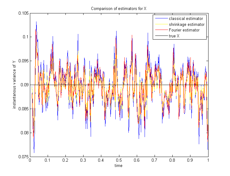
Figure 1. Comparison of estimators
3.3. Covariance of covariance estimation
Having reconstructed the path of the instantaneous covariance, we can now proceed with step (2), that is, the estimation of functions of the integrated covariance. To this end we plug the reconstructed path of the instantaneous covariance process into jump robust estimators of the form
where satisfies certain properties which are specified in Theorem 3.14 below.
Theorem 3.14.
-
•
Assume that the jumps of are of finite activity. Moreover, suppose that the paths of between two jumps are almost surely Hölder continuous with exponent .
-
•
Let and suppose that for some constant .
-
•
Let the conditions and or and with be in force and suppose that the instantaneous covariance process of defined by satisfies .
-
•
Let be such that exists and is continuous.
-
•
Suppose that satisfies either or and is additionally globally -Hölder continuous for .
-
•
Let and assume that for some constant .
Then
converges as stably in law to a -conditional Gaussian random variable defined on an extension of the original probability space with mean and covariance function given by
4. Proofs of the Asymptotic Properties of the Fourier Coefficients Estimator
In this section we provide the proofs of Theorem 3.4 and Corollary 3.6. Throughout always denotes some constant which can vary from line to line. Moreover, let us introduce the following notation
| (4.1) | ||||
| (4.2) |
4.1. Proof of Theorem 3.4
Proof.
We consider the one-dimensional case, i.e., , since the multi-dimensional case follows from it immediately in a methodological sense. Moreover, by the so called localization procedure as described in [3, Section 3] or [14, Section 4.4.1], we can strengthen assumption on together with Condition (3.3) to (see [3, Section 3]), that is, defined in (3.3), and are supposed to be uniformly bounded by a constant. Similarly, assumption on is strengthened to , that is, holds and the differential characteristics of the drift and the diffusion part of and (2.2), that is,
are bounded by a constant (compare [3, Assumption ] and [14, Assumption 4.4.7 (or (SK))]).
Let us denote by the elements of the Fourier basis
and let us split
into
where
and and are defined in (4.1) and (4.2). We divide the proof into several steps: the first step, which is subject of Proposition 4.1 below, consists in dealing with
| (4.3) |
As stated in Proposition 4.1 below, converges stably in law to the process , defined in (3.5).
For the central limit theorem the second step consists in showing that
converges in probability to . This can be shown similarly as in [14, Section 5.3.3, B]. Note that for the consistency result it is enough that
converges in probability to , which is implied by Riemann integrability.
In the third step we finally consider
which we split into , with
where denotes the diffusion part of defined in (3.2). For the central limit theorem to hold true, has to converge to in probability. To this end, it suffices to prove that
| (4.4) | ||||
| (4.5) |
holds true. Indeed, (4.4) implies (compare [14, Lemma 2.2.11])
and thus together with (4.5), we have . Both requirements (4.4) and (4.5) are met under the conditions on , and and the proof of (4.4) can be found in [3, Proof of Theorem 5.1] and (4.5) is shown in [14, Section 5.3.3, C]. For the consistency result only (4.4) has to be satisfied, which holds under the less restrictive assumptions and (see [3, Theorem 5.1]). Indeed, we only have to show that
which follows from the Cauchy-Schwarz inequality and (4.4), since
Finally, according to the assumptions or , respectively, we have for all
| (4.6) |
and
| (4.7) |
where
and is defined in (3.4). Due to or , respectively, the second term on the right hand side of (4.6) and (4.7) respectively tends to as for all . Since as , we deduce
and
respectively, which completes the proof. ∎
The following proposition is an application of [3, Proposition 4.1] or [14, Theorem 4.2.1]. The proof is omitted as it works along the lines of [3, Proposition 4.1]. Again we here only consider the one-dimensional case, i.e., and are one-dimensional and .
Proposition 4.1.
Assume that the process is càdlàg and bounded by a constant. Let be a function of at most polynomial growth. Then the sequence of processes defined in (4.3) is -tight. Moreover, if is even, then it converges stably in law to the process given componentwise for by
| (4.8) |
where
and is a -dimensional Brownian motion which is defined on an extension of the probability space and is independent of the -field .
4.2. Jump Robust Estimators - Proof of Corollary 3.6
The aim of this section is to specify classes of functions and conditions on the jumps such that condition or , respectively, is satisfied and such that the estimator given in (3.1) is robust to jumps. In particular, Corollary 3.6 is a consequence of the following proposition.
Proposition 4.2.
-
(i)
Let be continuous with as . Moreover, suppose that
(4.9) and . Then for all
(4.10) -
(ii)
Suppose that satisfies for some and some
(4.11) Moreover, let and assume that for all
(4.12) (4.13) and that as defined in (3.3) and is uniformly bounded.
-
(a)
If , then there exists some such that
(4.14) for all .
-
(b)
If , then
for all .
-
(a)
Remark 4.3.
-
(i)
Note that we can localize and consider processes for which (4.9) is automatically satisfied (see, e.g., [14, Lemma 3.4.5]). Assertion (i) then holds true for , which implies that is satisfied without further conditions on the characteristics of . Similarly the boundedness assumption on and in statement (ii) can also be obtained by localizing the original process.
- (ii)
Proof.
The first assertion is proved in [14, Lemma 3.4.6]. Concerning (ii), we shall distinguish the cases and and set without loss of generality . Due to the assumption on , we have
| (4.15) |
Applying Hölder’s inequality, we get for such that
Here, stands for each of the above expressions of the jumps and corresponds to or . Due to our assumptions on and and as a consequence of Hölder’s, Jensen’s and Burkholder-Davis-Gundy’s inequality the first expectation is bounded by a constant for all and .
If , we obtain a similar estimate by using Hölder and Burkholder-Davis-Gundy’s inequality, the fact that and (4.12):
The last equality follows from the fact that for , . Using these inequalities and setting equal to and , respectively, for some and , we can estimate (4.15) by
If , we can choose some such that this expression is simplified to
and if , we obtain
∎
4.2.1. Proof of Corollary 3.6
Proof.
Assertion (i) is a direct consequence of Theorem 3.4, Condition , Proposition 4.2 (i) and Remark 4.3 (i).
Again, in view of Theorem 3.4, the proof of the second statement consists in verifying Condition . Since , we can consider which is – since it is a càglàd process – locally bounded. By the localization procedure (see [14, Lemma 4.4.8]) we can therefore consider processes , for which and the diffusion characteristic are uniformly bounded and (4.13) and (4.12) for are satisfied, as required in Proposition 4.2 (ii).
This proposition then yields in the case
| (4.16) |
for some and in the case
By choosing in (4.16), is satisfied in both cases and the assertion follows. ∎
5. Proofs of the Asymptotic Properties of the Estimator for the Instantaneous Covariance Process
In this section we provide the proofs of Theorem 3.8 and Theorem 3.11. For the study of the asymptotic properties of the instantaneous covariance estimator given in (3.7), that is,
we need to analyze two different errors, namely
-
(i)
the error which comes from the fact that we use estimators for the Fourier coefficients instead of the true quantities, that is,
(5.1) -
(ii)
the error which we make by truncating the Fourier-Féjer sum, that is,
(5.2)
The term can be treated with well known deterministic results on Fourier-Féjer series, whereas the statistical error needs to be decomposed in several parts and handled with probabilistic methods, in particular limit theorems for triangular arrays. To apply these methods let us first remark that can be written as
| (5.3) |
where denotes the Féjer kernel defined by
| (5.4) |
Using this representation, the term given in (5.1) can now be written as
This can be further decomposed into , where
| (5.5) | ||||
| (5.6) | ||||
| (5.7) | ||||
| (5.8) |
with and given in (4.1) and (4.2). In view of this decomposition, we start with the following lemma which deals with convergence of Riemann sums for the Féjer kernel and which is crucial for studying asymptotic properties of the instantaneous covariance estimators.
Lemma 5.1.
Let and denote
and consider the Féjer kernel given in (5.4). Moreover, let and suppose that for some constant and let be a -Hölder continuous function with . Then, the following identities holds true:
| (5.9) | ||||
| (5.10) | ||||
| (5.11) |
Furthermore, we have the following error estimates:
Remark 5.2.
Proof.
We have convergence of the Riemann sums in (5.9) to the corresponding integral if the grid becomes finer within the zeros of . Since the distance between zeros is ( for the zeros closest to the origin), this is the case if only if . By the same argument the left hand side of (5.10) and (5.11) converges to the corresponding integrals if and only if . The assertion then follows from the following calculation
Concerning the error estimates, we have due to the mean value theorem
with some . Using again the mean value theorem, we can further estimate
Since
and since
it follows that
Hence, we have
which yields the assertion. Concerning
we can estimate it by
∎
5.1. Consistency - Proof of Theorem 3.8
Using the above lemma we can now proceed to establish consistency of the estimator given in (3.7).
Proof.
Similar as in [3] or [14, Section 4.4.1] and the proof of Theorem 3.4, we strengthen assumption together with Condition (3.3) to boundedness of and . As already explained in the introduction of this section, we decompose
By Féjer’s theorem the term converges to a.s., since is supposed to have càdlàg paths.
As a consequence of the proof of Theorem 3.11 below, the term converges to in probability under the assumptions () and ().
Again by the càdlàg property and the boundedness of (recall the boundedness condition on and the fact that has at most polynomial growth) and the assumption , converges a.s. to by Riemann integrability (cf. Lemma 5.1).
Finally we have to focus on the , which we decompose into
where is defined in (3.2). The second term converges in probability to , since it can be estimated by
and we have (see the proof of [3, Lemma 5.3, Lemma 5.4]). Writing and , where is defined in (3.4), we have
| (5.12) | ||||
Since as and since can be estimated by
which converges to for all due to Assumption , (5.12) tends to as well. ∎
5.2. Central Limit Theorem - Proof of Theorem 3.11
This section is dedicated to the proof of the central limit theorem for (functions of) the instantaneous covariance.
Proof.
Similarly as in the proof of Theorem 3.4, we strengthen the assumption to , that is, , defined in (3.3), and the differential characteristics of the drift and the diffusion part of and (2.2) are bounded by a constant. Analogously to the proof of Theorem 3.8 we decompose
into , where , are defined in (5.5) - (5.8) and is here given by
Denoting by the set
we have the following estimate for :
| (5.13) |
Due to the assumption that has no fixed time of discontinuity, the first term converges to . By the assumption of finite activity jumps and Hölder continuity of between two jumps, we have
for some finitely valued number (depending on ) (compare [20, Eq. 13] and [33]). Since by assumption, the second term in the above decomposition thus also converges to .
Due to Lemma 5.1 and again the assumption of finite activity jumps and Hölder continuity of between two jumps , can be estimated by
which converges to , since again as a consequence of the assumption . A similar decomposition as in (5.13) yields .
Let us now consider , which we decompose into
In view of Lemma [14, Lemma 2.2.11] it is sufficient to prove that
| (5.14) | |||
| (5.15) |
and
| (5.16) |
where
Let us first focus on . By [3, Lemma 5.3 and Lemma 5.4]) and no fixed time of discontinuity of we have
and we can therefore estimate (5.14) by
which converges to due to Lemma 5.1.
Concerning (5.15), it is possible to decompose
where for all , and with (see [14, Section 5.3.3, C]. Then
converges due to Lemma 5.1 and thus yields (5.15). Condition (5.16) follows from the assumption for and a similar estimate as in (5.12).
Let us now turn to , which we write as
where
Since , we also have
Moreover,
Thus we have
Due to Lemma 5.1 and Remark 5.2 the limit of this expression is given by
In view of Theorem [15, Theorem IX.7.28] it remains to verify that
| (5.17) |
for all . By the Cauchy-Schwarz inequality we have
By definition of and the polynomial growth of , we can further estimate
Taking again the polynomial growth of into account, there exists some such that
where . Thus
Since this tends to , we can estimate (5.17) by
where convergence to follows from Lemma 5.1 and the above estimate for
hence Equation (5.17) is verified. Moreover, similarly as in the proof of [3, Proposition 4.1], we have
and
for any bounded martingale which is orthogonal to the Brownian motion . The assertion is now implied by all these estimates and [15, Theorem IX.7.28]. ∎
6. Covariance of Covariance Estimation - Proof of Theorem 3.14
In this section we prove Theorem 3.14, i.e., a central limit theorem for the estimator of the integrated covariance of obtained from the reconstructed path .
Proof.
Let us decompose
| (6.1) |
In view [14, Theorem 5.3.5 and 5.3.6], the second term converges to the stated Gaussian random variable. Hence we only have to prove that the first term converges to in probability. Due to the assumptions on , it can be estimated by
Denoting by the set
| (6.2) |
we further split the above expression into
Due to the assumption of finite activity jumps, the second sum contains a.s. only finitely many summands and thus converges to a.s. since . By Lemma 6.1 below, the relation between and and the condition on , the first sum converges to in probability. ∎
Lemma 6.1.
Proof.
By localizing we can assume that is uniformly bounded. In fact, consider a localizing sequence
and the processes
where is uniformly bounded by definition. Moreover, define
and
Then the left hand side of
tends to , if the second term on the right hand side does. Therefore, we can assume uniform boundedness of .
By the mean value theorem we obtain the identity
where is a random variable satisfying . Due to the continuity assumption on and boundedness of , (6.3) converges to in probability if
An inspection of the proof of Theorem 3.11 reveals that this is the case if the conditions between , and are satisfied. Indeed, we split in the same parts as in Theorem 3.11, that is,
where , are defined in (5.5) - (5.8) and is here given by
We start by showing
By the assumption of finitely many jumps and -Hölder continuity between two jumps, we can find a uniform (in ) bound (depending on ) such that
Indeed, this is due to the fact that no jump occurs in , the condition on and , namely for some constant and , and the way how the Féjer kernel declines, in particular that
holds true. Hence we obtain
which tends to due to the relation of and .
Similarly we have a uniform (in ) convergence rate for to which is of order . The same arguments thus yield
Concerning
it suffices to show that
By the relation of and , this then follows from the fact that
for all . This latter property then follows from uniform convergence (in ) of
In order to prove
we estimate the -norm of this expression by
which converges to due to the relation between and . The last inequality is a consequence of Lemma 5.1, where the assertion of (5.10) can be extended to uniform convergence.
∎
Appendix A Simulation results
In this section we illustrate our theoretical results in the case of a multivariate affine model, where both the log-price and the instantaneous covariance process can jump. More precisely, we consider a multivariate Bates-type model (compare, e.g., [9, 10, 17], of the form
where
-
•
is a -dimensional Brownian motion correlated with the matrix of Brownian motions such that , where such that and is a -dimensional Brownian motion independent of ,
-
•
is the random measure associated with the jumps of , whose compensator is given by , where and denotes the Gaussian density with mean and standard deviation ,
-
•
is the random measure associated with the jumps of , whose compensator is given by , where and denotes the density of the exponential distribution with parameter ,222We here only suppose that can jump.
-
•
the drift of is given by and
-
•
the parameters of satisfy , , such that
Note that the truncation function of is here chosen to be .
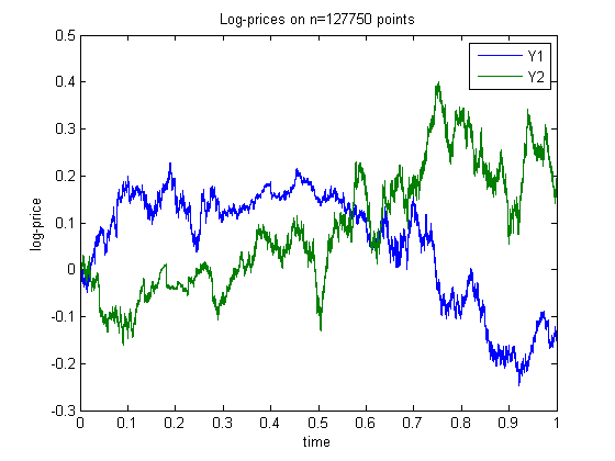
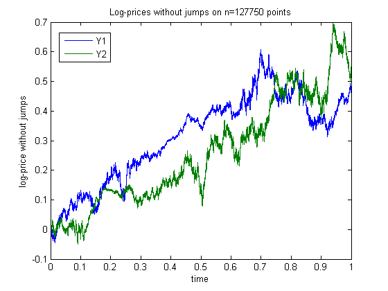
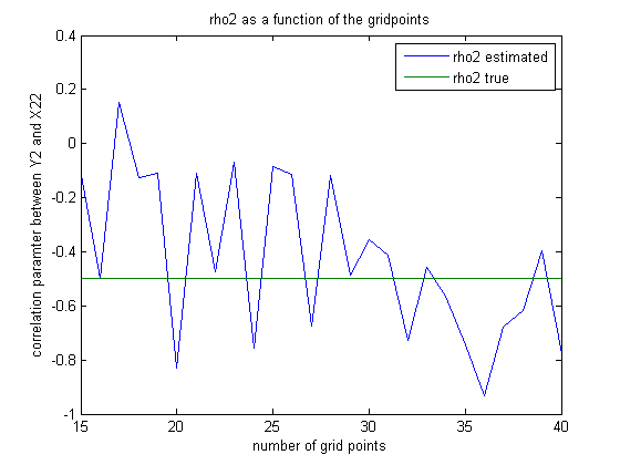
As described in Section 1.1 and Section 2.2 we aim to recover the instantaneous covariance process and the parameters and from observations of . In order to be in accordance with market specifications, we simulate and on grid points, which corresponds to 1 year () of 1-minute data. For our numerical simulation, we consider the case and use the following parameter values:
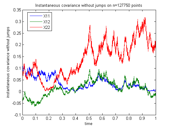
In order to illustrate in particular that our estimator is robust to small and frequent jumps, the jump intensity of both log-prices is chosen to be quite high. Figure 2 below show simulated trajectories of the log-price and the instantaneous covariance process, where the jumps are removed in the second graph in each case.
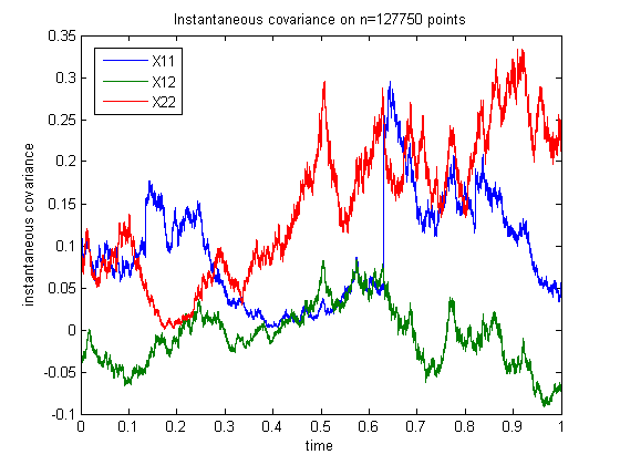
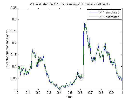
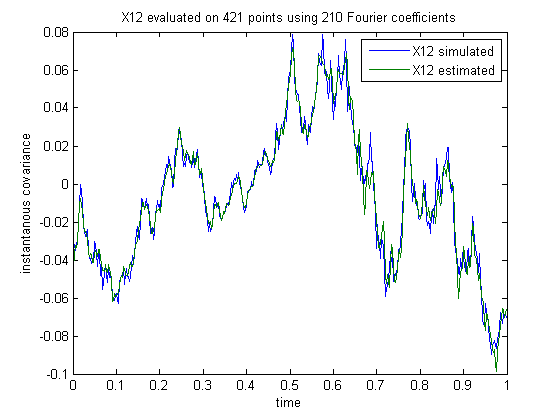
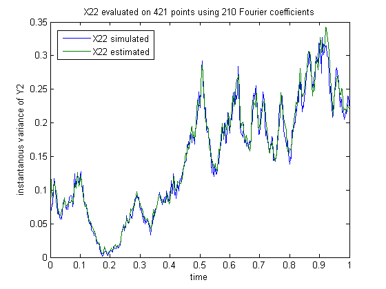
A comparison between the reconstructed and simulated trajectories of the instantaneous covariance process is shown in Figure 3. These figures illustrate that – even in the case of (frequent) jumps in the log-price and in the variance (as it is the case for ) – the paths of can be recovered very well. For the reconstruction of the trajectories of we choose Fourier coefficients, which corresponds to the choice and , as specified in Theorem 3.11. This is a reasonable choice in view of an acceptable bias and a rather small variance. Both, the simulated as well as the reconstructed trajectories are evaluated at points. In our concrete implementation the estimator for the Fourier coefficients (3.1) is based on the Tauchen-Todorov specification of the function , that is,
In this case
and is obtained by
The reconstructed trajectories of are then used to estimate the parameters and . To this end, we use the power variation estimators, i.e.,
where
These quantities are estimators for the power (co)variation of and . Indeed we have under the assumptions of Theorem 3.14
as . The formulas on the right hand sides follow from the expressions for the absolute moments of the bivariate Gaussian distribution (see, e.g.,[24]) and denotes the Gaussian hypergeometric function.
The estimators for and can now be constructed via
where we discretize the corresponding integrals in and and instead of . In our simulation study, we choose in and in for and respectively. This is due to the fact that exhibits jumps and taking a lower power reduces the contribution of jumps in the power variation. In , and are chosen to be . Figure 4 and 5 show the estimated values for and as a function of the grid points . As a consequence of Theorem 3.14, the grid corresponding to has to be coarsened considerably with respect to the initial gridding with points (of order or even more depending on the power used). For this reason the number of grid points shown in the graphs is rather small. Nevertheless the estimation results are good approximations of the true parameter values and can further be improved by increasing and thus in turn also .
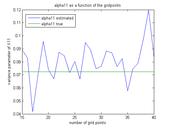
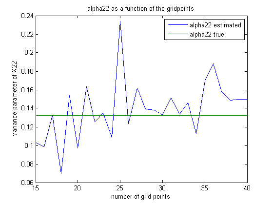
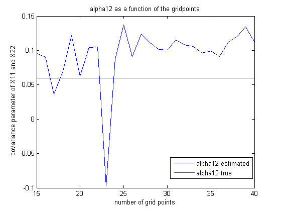
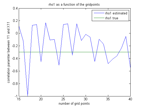
References
- [1] A. Alvarez, F. Panloup, M. Pontier, and N. Savy. Estimation of the instantaneous volatility. Stat. Inference Stoch. Process., 15(1):27–59, 2012.
- [2] F. Bandi and R. Renò. Nonparametric stochastic volatility. Working paper, 2011.
- [3] O. E. Barndorff-Nielsen, S. E. Graversen, J. Jacod, M. Podolskij, and N. Shephard. A central limit theorem for realised power and bipower variations of continuous semimartingales. In From stochastic calculus to mathematical finance, pages 33–68. Springer, Berlin, 2006.
- [4] O. E. Barndorff-Nielsen, S. E. Graversen, and N. Shephard. Power variation and stochastic volatility: a review and some new results. J. Appl. Probab., 41A:133–143, 2004. Stochastic methods and their applications.
- [5] O. E. Barndorff-Nielsen and N. Shephard. Power and bipower variation with stochastic volatility and jumps. J. of Financial Econometrics, 2(1):1–37, 2004.
- [6] O. E. Barndorff-Nielsen, N. Shephard, and M. Winkel. Limit theorems for multipower variation in the presence of jumps. Stochastic Process. Appl., 116(5):796–806, 2006.
- [7] O. E. Barndorff-Nielsen and A. E. D. Veraart. Stochastic volatility of volatility and variance risk premia. Journal of Financial Econometrics, 11(1):1–46, 2012.
- [8] E. Barucci and M. E. Mancino. Computation of volatility in stochastic volatility models with high frequency data. Int. J. Theor. Appl. Finance, 13(5):767–787, 2010.
- [9] C. Cuchiero, D. Filipović, E. Mayerhofer, and J. Teichmann. Affine processes on positive semidefinite matrices. Ann. Appl. Probab., 21(2):397–436, 2011.
- [10] J. Da Fonseca, M. Grasselli, and C. Tebaldi. A multifactor volatility Heston model. Quant. Finance, 8(6):591–604, 2008.
- [11] J. Fan and Y. Wang. Spot volatility estimation for high-frequency data. Stat. Interface, 1(2):279–288, 2008.
- [12] V. Genon-Catalot, C. Laredo, and D. Picard. Nonparametric estimation of the diffusion coefficient by wavelets methods. Scand. J. Statist., 19(4):317–335, 1992.
- [13] J. Jacod. Asymptotic properties of realized power variations and related functionals of semimartingales. Stochastic Process. Appl., 118(4):517–559, 2008.
- [14] J. Jacod and P. Protter. Discretization of processes, volume 67 of Stochastic Modelling and Applied Probability. Springer, Heidelberg, 2012.
- [15] J. Jacod and A. N. Shiryaev. Limit theorems for stochastic processes, volume 288 of Fundamental Principles of Mathematical Sciences. Springer-Verlag, Berlin, second edition, 2003.
- [16] D. Kristensen. Nonparametric filtering of the realized spot volatility: a kernel-based approach. Econometric Theory, 26(1):60–93, 2010.
- [17] M. Leippold and F. Trojani. Asset pricing with matrix jump diffusions. SSRN eLibrary, 2008.
- [18] G. G. Lorentz. Approximation of functions. Chelsea Publishing Co., New York, second edition, 1986.
- [19] P. Malliavin and M. E. Mancino. Fourier series method for measurement of multivariate volatilities. Finance Stoch., 6(1):49–61, 2002.
- [20] P. Malliavin and M. E. Mancino. A Fourier transform method for nonparametric estimation of multivariate volatility. Ann. Statist., 37(4):1983–2010, 2009.
- [21] C. Mancini. Non-parametric threshold estimation for models with stochastic diffusion coefficient and jumps. Scand. J. Stat., 36(2):270–296, 2009.
- [22] C. Mancini. The speed of convergence of the threshold estimator of integrated variance. Stochastic Process. Appl., 121(4):845–855, 2011.
- [23] P. A. Mykland and L. Zhang. Inference for volatility-type objects and implications for hedging. Stat. Interface, 1(2):255–278, 2008.
- [24] S. Nabeya. Absolute moments in -dimensional normal distribution. Ann. Inst. Statist. Math., Tokyo, 3:2–6, 1951.
- [25] M. Podolskij. New theory on estimation of integrated volatility with applications. PhD Thesis, Ruhr-Universitaet Bochum, 2006.
- [26] M. Podolskij and M. Vetter. Estimation of volatility functionals in the simultaneous presence of microstructure noise and jumps. Bernoulli, 15(3):634–658, 2009.
- [27] N. Privault and A. Réveillac. Stein estimation for the drift of Gaussian processes using the Malliavin calculus. Ann. Statist., 36(5):2531–2550, 2008.
- [28] M. Reiß. Asymptotic equivalence for nonparametric regression with multivariate and random design. Ann. Stat., 36(4):1957–1982, 2008.
- [29] V. Todorov and G. Tauchen. The realized Laplace transforms of volatility. Preprint, 2011.
- [30] M. Vetter. Estimation of correlation for continuous semimartingales. Scandinavian Journal of Statistics, 39(4):757–771, 2012.
- [31] D. C. Wang and P. A. Mykland. The estimation of leverage effect with high frequency data. Preprint, 2012.
- [32] J. H. C. Woerner. Power and multipower variation: inference for high frequency data. In A. N. Shiryaev, M. R. Grossinho, P. E. Oliveira, and M. L. Esquivel, editors, Stochastic Finance, pages 343–364. Springer US, 2006.
- [33] M. Zamansky. Classes de saturation de certains procédés d’approximation des séries de Fourier des fonctions continues et applications à quelques problèmes d’approximation. Ann. Sci. École. Norm. Sup. (3), 66:19–93, 1949.