Deep Learning for Detecting Robotic Grasps

Abstract

We consider the problem of detecting robotic grasps in an RGB-D view of a scene containing objects. In this work, we apply a deep learning approach to solve this problem, which avoids time-consuming hand-design of features. This presents two main challenges. First, we need to evaluate a huge number of candidate grasps. In order to make detection fast and robust, we present a two-step cascaded system with two deep networks, where the top detections from the first are re-evaluated by the second. The first network has fewer features, is faster to run, and can effectively prune out unlikely candidate grasps. The second, with more features, is slower but has to run only on the top few detections. Second, we need to handle multimodal inputs effectively, for which we present a method that applies structured regularization on the weights based on multimodal group regularization. We show that our method improves performance on an RGBD robotic grasping dataset, and can be used to successfully execute grasps on two different robotic platforms.

Keywords: Robotic Grasping, deep learning, RGB-D multi-modal data, Baxter, PR2, 3D feature learning.

I Introduction

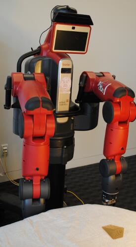
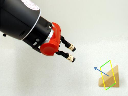
Robotic grasping is a challenging problem involving perception, planning, and control. Some recent works [54, 56, 28, 67] address the perception aspect of this problem by converting it into a detection problem in which, given a noisy, partial view of the object from a camera, the goal is to infer the top locations where a robotic gripper could be placed (see Figure 1). Unlike generic vision problems based on static images, such robotic perception problems are often used in closed loop with controllers, so there are stringent requirements on performance and computational speed. In the past, hand-designing features has been the most popular method for several robotic tasks [40, 32]. However, this is cumbersome and time-consuming, especially when we must incorporate new input modalities such as RGB-D cameras.

Recent methods based on deep learning [1] have demonstrated state-of-the-art performance in a wide variety of tasks, including visual recognition [35, 60], audio recognition [39, 41], and natural language processing [12]. These techniques are especially powerful because they are capable of learning useful features directly from both unlabeled and labeled data, avoiding the need for hand-engineering.

However, most work in deep learning has been applied in the context of recognition. Grasping is inherently a detection problem, and previous applications of deep learning to detection have typically focused on specific vision applications such as face detection [45] and pedestrian detection [57]. Our goal is not only to infer a viable grasp, but to infer the optimal grasp for a given object that maximizes the chance of successfully grasping it, which differs significantly from the problem of object detection. Thus, the first major contribution of our work is to apply deep learning to the problem of robotic grasping, in a fashion which could generalize to similar detection problems.

Figure 1: Detecting robotic grasps: Left: A cluttered lab scene labeled with rectangles corresponding to robotic grasps for objects in the scene. Green lines correspond to robotic gripper plates. We use a two-stage system based on deep learning to learn features and perform detection for robotic grasping. Center: Our Baxter robot “Yogi” successfully executing a grasp detected by our algorithm. Right: The grasp detected for this case, in the RGB (top) and depth (bottom) images obtained from Kinect.

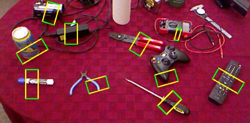
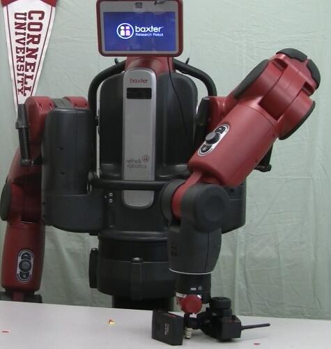
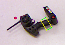
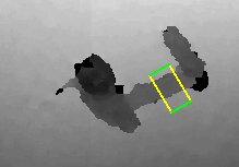
The second major contribution of our work is to propose a new method for handling multimodal data in the context of feature learning. The use of RGB-D data, as opposed to simple 2D image data, has been shown to significantly improve grasp detection results [28, 14, 56]. In this work, we present a multimodal feature learning algorithm which adds a structured regularization penalty to the objective function to be optimized during learning. As opposed to previous works in deep learning, which either ignore modality information at the first layer (i.e., encourage all features to use all modalities) [59] or train separate first-layer features for each modality [43, 61], our approach allows for a middle-ground in which each feature is encouraged to use only a subset of the input modalities, but is not forced to use only particular ones.

We also propose a two-stage cascaded detection system based on deep learning. Here, we use fewer features for the first pass, providing faster, but only approximately accurate detections. The second pass uses more features, giving more accurate detections. In our experiments, we found that the first deep network, with fewer features, was better at avoiding overfitting but less accurate. We feed the top-ranked rectangles from the first layer into the second layer, leading to robust early rejection of false positives. Unlike manually designed two-step features as in [28], our method uses deep learning, which allows us to learn detectors that not only give higher performance, but are also computationally efficient.

We test our approach on a challenging dataset, where we show that our algorithm improves both recognition and detection performance for grasping rectangle data. We also show that our two-stage approach is not only able to match the performance of a single-stage system, but, in fact, improves results while significantly reducing the computational time needed for detection.

In summary, the contributions of this paper are:

• We present a deep learning algorithm for detecting robotic grasps. To the best of our knowledge, this is the first work to do so.

• In order to handle multimodal inputs, we present a new way to apply structured regularization to the weights to these inputs based on multimodal group regularization.

• We present a multi-step cascaded system for detection, significantly reducing its computational cost.

• Our method outperforms the state-of-the-art for rectangle-based grasp detection, as well as previous deep learning algorithms.

• We implement our algorithm on both a Baxter and a PR2 robot, and show success rates of 84% and 89%, respectively, for executing grasps on a highly varied set of objects.

The rest of the paper is organized as follows: We discuss related work in Section II. We present our two-step cascaded detection system in Section III, and some additional details in Section IV. We then describe our feature learning algorithm and structured regularization method in Section V. We present our experiments in Section VI, and discuss results in Section VII. We then present experiments on both Baxter and PR2 robots in Section VIII. We present several interesting directions for future work in Section IX, then conclude in Section X.

II Related Work

II-A Robotic Grasping

In this section, we will focus on perception- and learning-based approaches for robotic grasping. For a more complete review of the field, we refer the reader to review papers by Bohg et al. [4], Sahbani et al. [53], Bicchi and Kumar [2] and Shimoga [58].

Most works define a “grasp” as an end-effector configuration which achieves partial or complete form- or force-closure of a given object. This is a challenging problem because it depends on the pose and configuration of the robotic gripper as well as the shape and physical properties of the object to be grasped, and typically requires a search over a large number of possible gripper configurations. Early works [34, 44, 49] focused on testing for form- and force-closure, and synthesizing grasps fulfilling these properties according to some hand-designed “quality score” [17]. More recent works have refined these definitions [50]. These works assumed full knowledge of object shape and physical properties.

Grasping Given 3D Model: Fast synthesis of grasps for known 3D models remains an active research topic [14, 20, 65], with recent methods using advanced physical simulation to find optimal grasps. Gallegos et al. [18] performed optimization of grasps given both a 3D model of the object to be grasped and the desired contact points for the robotic gripper. Pokorny et al. [48] define spaces of graspable objects, then map new objects to these spaces to discover grasps. However, these works are only applicable when the full 3D model of the object is exactly known, which may not be the case when a robot is interacting with a new environment. We note that some of these physics-based approaches might be combined with our approach in a multi-pass system, discussed further in Sec. IX.

Sensing for Grasping: In a real-world robotic setting, a robot will not have full knowledge of the 3D model and pose of an object to be grasped, but rather only incomplete information from some set of sensors such as color or depth cameras, tactile sensors, etc. This makes the problem of grasping significantly more challenging [4], as the algorithm must use more limited and potentially noisier information to detect a good grasp. While some works [10, 46] simply attempt to estimate the poses of known objects and then apply full-model grasping algorithms based on these results, others avoid this assumption, functioning on novel objects which the algorithm has not seen before.

Such works often made use of other simplifying assumptions, such as assuming that objects belong to one of a set of primitive shapes [47, 6], or are planar [42]. Other works produced impressive results for specific cases, such as grasping the corners of towels [40]. While such works escape the assumption of a fully-known object model, hand-coded grasping rules have a hard time dealing with the wide range of objects seen in real-world human environments, and are difficult and time-consuming to create.

Learning for Grasping: Machine learning methods have proven effective for a wide range of perception problems [64, 22, 38, 59, 3], allowing a perception system to learn a mapping from some feature set to various visual properties. Early work by Kamon et al. [31] showed that learning approaches could also be applied to the problem of grasping from vision, introducing a learning component to grasp quality scores.

Recent works have employed richer features and learning methods, allowing robots to grasp known objects which might be partially occluded [27] or in an unknown pose [13] as well as fully novel objects which the system has not seen before [54]. Here, we will address the latter case. Earlier work focused on detecting only a single grasping point from 2D partial-view data, using heuristic methods to determine a gripper pose based on this point. [55]. The use of 3D data was shown to significantly improve these results [56] thanks to giving direct physical information about the object in question. With the advent of low-cost RGB-D sensors such as the Kinect, the use of depth data for robotic grasping has become ubiquitous.

Several other works attempted to use the learning algorithm to more fully constrain the detected grasps. Ekvall and Kragic [15] and Huebner and Kragic [23] used shape-based approximations as bases for learning algorithms which directly gave an approach vector. Le et al. [36] treated grasp detection as a ranking problem over sets of contact points in image space. Jiang et al. [28] represented a grasp as a 2D oriented rectangle in image space, with two edges corresponding to the gripper plates, using surface normals to determine the grasp approach vector. These approaches allow the detection algorithm to detect more exactly the gripper pose which should be used for grasping. In this work, we will follow the rectangle-based method.

Learning-based approaches have shown impressive results in grasping novel objects, showing that learning some parameters of the detection system can outperform human tuning. However, these approaches still require a significant degree of hand-engineering in the form of designing good input features.

Other Applications with RGBD Data. Due to the availability of inexpensive depth sensors, RGB-D data has been a significant research focus in recent years for various robotics applications. For example, Jiang et al. [30] consider robotic placement of objects, while Teuliere and Marchand [63] used RGB-D data for visual servoing. Several works, including those of Endres et al. [16] and Whelan et al. [66] have extended and improved Simultaneous Localization and Mapping (SLAM) for RGB-D data. Object detection and recognition has been a major focus in research on RGB-D data [11, 33, 7]. Most such works use hand-engineered features such as [52]. The few works that perform feature learning for RGB-D data [59, 3] largely ignore the multimodal nature of the data, not distinguishing the color and depth channels. Here, we present a structured regularization approach which allows us to learn more robust features for RGB-D and other multimodal data.

II-B Deep Learning

Deep learning approaches have demonstrated the ability to learn useful features directly from data for a wide variety of tasks. Early work by Hinton and Salakhutdinov [22] showed that a deep network trained on images of hand-written digits will learn features corresponding to pen-strokes. Later work using localized convolutional features [38] showed that these networks learn features corresponding to object parts when trained on natural images. This demonstrates that even the basic features learned by these systems will adapt to the data given. In fact, these approaches are not restricted to the visual domain, but rather have been shown to learn useful features for a wide range of domains, such as audio [39, 41] and natural language data [12].

Deep Learning for Detection: However, the vast majority of work in deep learning focuses on classification problems. Only a handful of previous works have applied these methods to detection problems [45, 37, 9]. For example, Osadchy et al. [45] and LeCun et al. [37] applied a deep energy-based model to the problem of face detection, Sermanet et al. [57] applied a convolutional neural network for pedestrian detection, and Coates et al. [9] used a deep learning approach to detect text in images. Girshick et al. [19] used learned convolutional features over image regions for object detection, while Szegedy et al. [62] used a multi-scale approach based on deep networks for the same task.

All these approaches focused on object detection and similar problems, in which the goal is to find a bounding box which tightly contains the item to be detected, and for each item, all valid bounding boxes will be similar. However, in robotic grasp detection, there may be several valid grasps for an object in different regions, making it more important to select the one with the highest chance success. In addition, orientation matters much more to robotic grasp detection, as most grasps will only be viable for a small subset of the possible gripper orientations. Our approach to grasp detection will also generalize across object classes, and even to classes never seen before by the system, as opposed to the class-specific nature of object detection.

Figure 2: Detecting and executing grasps: From left to right: Our system obtains an RGB-D image from a Kinect mounted on the robot, and searches over a large space of possible grasps, for which some candidates are shown. For each of these, it extracts a set of raw features corresponding to the color and depth images and surface normals, then uses these as inputs to a deep network which scores each rectangle. Finally, the top-ranked rectangle is selected and the corresponding grasp is executed using the parameters of the detected rectangle and the surface normal at its center. Red and green lines correspond to gripper plates, blue in RGB-D features indicates masked-out pixels.

Multimodal Deep Learning: Recent works in deep learning have extended these methods to handle multiple modalities of input data, such as audio and video [43], text and image data [61], and even RGB-D data [59, 3]. However, all of these approaches have fallen into two camps - either learning completely separate low-level features for each modality [43, 61], or simply concatenating the modalities [59, 3]. The former approaches have proven effective for data where the basic modalities differ significantly, such as the aforementioned case of text and images, while the latter is more effective in cases where the modalities are more similar, such as RGB-D data.

For some new combinations of modalities and tasks, it may not be clear which of these approaches will give better performance. In fact, in the ideal feature set, different features may use different subsets of the modalities. In this work, we will give a structured regularization method which guides the learning algorithm to select such subsets, without imposing hard constraints on network structure.

Structured Learning and Structured Regularization: Several approaches have been proposed which attempt to use a specially-designed regularization function to impose structure on a set of learned parameters without directly enforcing it. Jalali et al. [26] used a group regularization function in the multitask learning setting, where one set of features is used for multiple tasks. This function applies high-order regularization separately to particular groups of parameters. Their function regularized the number of features used for each task in a set of multi-class classification tasks solved by softmax regression. Intuitively, this encodes the belief that only some subset of the input features will be useful for each task, but this set of useful features might vary between tasks.

A few works have also explored the use of structured regularization in deep learning. The Topographic ICA algorithm [24] is a feature-learning approach that applies a similar penalty term to feature activations, but not to the weights themselves. Coates and Ng [8] investigate the problem of selecting receptive fields, i.e., subsets of the input features to be used together in a higher-level feature. The structure of the network is learned first, then fixed before learning the parameters of the network.

Figure 3: Illustration of our two-stage detection process: Given an image of an object to grasp, a small deep network is used to exhaustively search potential rectangles, producing a small set of top-ranked rectangles. A larger deep network is then used to find the top-ranked rectangle from these candidates, producing a single optimal grasp for the given object.

III Deep Learning for Grasp Detection:
System and Model

In this work, we will present an algorithm for robotic grasp detection from a single RGB-D view. Our approach will be based on machine learning, but distinguish itself from previous approaches by learning not only the weights used to rank prospective grasps, but also the features used to rank them, which were previously hand-engineered.

We will do this using deep learning methods, learning a set of RGB-D features which will be extracted from each candidate grasp, then used to score that grasp. Our approach will include a structured multimodal regularization method which improves the quality of the features learned from RGB-D data without constraining network structure.

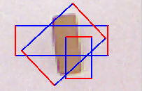
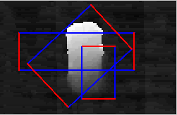
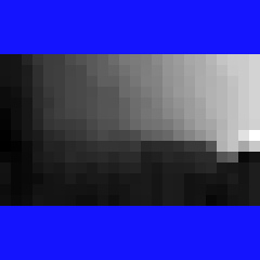
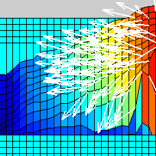
In our system for robotic grasping, as shown in Fig. 2, the robot first obtains an RGB-D image of the scene containing objects to be grasped. A small deep network is used to score potential grasps in this image, and a small candidate set of the top-ranked grasps is provided to a larger deep network, which yields a single best-ranked grasp.

In this work, we will represent potential grasps using oriented rectangles in the image plane as seen on the left in Fig. 2, with one pair of parallel edges corresponding to the robotic gripper [28]. Each rectangle is thus parameterized by the X and Y coordinates of its upper-left corner, its width, height, and orientation in the image plane, giving a five-dimensional search space for potential grasps. Grasps will be ranked based on features extracted from the RGB-D image region contained inside their corresponding rectangle, aligned to the gripper plates, as seen in the center of Fig. 2.

To translate a rectangle such as that shown on the right in Fig. 2 into a gripper pose for grasping we find the point with the minimum depth inside the central third (horizontally) of the rectangle. We then use the averaged surface normal around this point to determine the approach vector for the gripper. The orientation of the detected rectangle is translated to a rotation around this vector to orient the gripper. We use the X-Y coordinates of the rectangle center along with the depth of the closest point to determine a grasping point in the robot’s coordinate frame. We compute a pre-grasp position by shifting 10 cm back from the grasping point along this approach vector and position the gripper at this point. We then approach the object along the approach vector and grasp it.

Using a standard feature learning approach such as sparse auto-encoder [21], a deep network can be trained for the problem of grasping rectangle recognition (i.e., does a given rectangle in image space correspond to a valid robotic grasp?). However, in a real-world robotic setting, our system needs to perform detection (i.e., given an image containing an object, how should the robot grasp it?). This task is significantly more challenging than simple recognition.

Figure 4: Deep network and auto-encoder: Left: A deep network with two hidden layers, which transform the input representation, and a logistic classifier at the top layer, which uses the features from the second hidden layer to predict the probability of a grasp being feasible. Right: An auto-encoder, used for pretraining. A set of weights projects input features to a hidden layer. The same weights are then used to project these hidden unit outputs to a reconstruction of the inputs. In the sparse auto-encoder (SAE) algorithm, the hidden unit activations are also penalized.

Two-stage Cascaded Detection: In order to perform detection, one naive approach could be to consider each possible oriented rectangle in the image (perhaps discretized to some level), and evaluate each rectangle with a deep network trained for recognition. However, such near-exhaustive search of possible rectangles (based on positions, sizes, and orientations) can be quite expensive in practice for real-time robotic grasping.

Motivated by multi-step cascaded approaches in previous work [28, 64], we instead take a two-stage approach to detection: First, we use a reduced feature set to determine a set of top candidates. Then, we use a larger, more robust feature set to rank these candidates.

However, these approaches require the design of two separate sets of features. In particular, it can be difficult to manually design a small set of first-stage features which is both quick to compute and robust enough to produce a good set of candidate detections for the second stage. Using deep learning allows us to circumvent the costly manual design of features by simply training networks of two different sizes, using the smaller for the exhaustive first pass, and the larger to re-rank the candidate detection results.

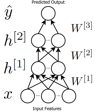
Model: To detect robotic grasps from the rectangle representation, we model the probability of a rectangle $G^{(t)}$, with features $x^{(t)}\in\mathbb{R}^{N}$ being graspable, using a random variable $\hat{y}^{(t)}\in\{0,1\}$ which indicates whether or not we predict $G^{(t)}$ to be graspable. We use a deep network, as shown in Fig. 4-left, with two layers of sigmoidal hidden units $h^{[1]}$ and $h^{[2]}$, with $K_{1}$ and $K_{2}$ units per layer, respectively. A logistic classifier over the outputs of the second-layer hidden units then predicts $P(\hat{y}^{(t)}|x^{(t)};\Theta)$, so chosen because ground-truth graspability is represented as binary. Each layer $\ell$ will have a set of weights $W^{[\ell]}$ mapping from its inputs to its hidden units, so the parameters of our model are $\Theta=\{W^{[1]},W^{[2]},W^{[3]}\}$. Each hidden unit forms output by a sigmoid $\sigma(a)=1/(1+\exp(-a))$ over its weighted input:

$$h_{j}^{[1](t)} =\sigma\left(\sum_{i=1}^{N}x_{i}^{(t)}W^{[1]}_{i,j}\right)$$

$$h_{j}^{[2](t)} =\sigma\left(\sum_{i=1}^{K_{1}}h_{i}^{[1](t)}W^{[2]}_{i,j}\right)$$

$$P(\hat{y}^{(t)}=1|x^{(t)};\Theta) =\sigma\left(\sum_{i=1}^{K_{2}}h_{i}^{[2](t)}W^{[3]}_{i}\right)$$ (1)

III-A Inference and Learning

During inference, our goal is to find the single grasping rectangle with the maximum probability of being graspable for some new object. With $G$ representing a particular grasping rectangle position, orientation, and size, we find this best rectangle as:

$$G^{*} =\underset{G}{\mbox{arg max }}P(\hat{y}^{(t)}=1|\phi(G);\Theta)$$ (2)

Here, the function $\phi$ extracts the appropriate input representation for rectangle $G$.

During learning, our goal is to learn the parameters $\Theta$ that optimize the recognition accuracy of our system. Here, input data is given as a set of pairs of features $x^{(t)}\in\mathbb{R}^{N}$ and ground-truth labels $y^{(t)}\in\{0,1\}$ for $t=1,\ldots,M$. As in most deep learning works, we use a two-phase learning approach.

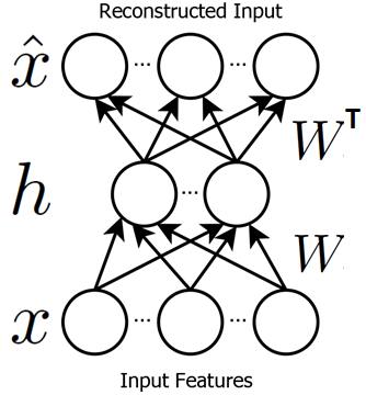
In the first phase, we will use unsupervised feature learning to initialize the hidden-layer weights $W^{[1]}$ and $W^{[2]}$. Pre-training weights this way is critical to avoid overfitting. We will use a variant of a sparse auto-encoder (SAE) [21], as illustrated in Fig. 4-right. We define $g(h)$ as a sparsity penalty function over hidden unit activations, with $\lambda$ controlling its weight. With $f(W)$ as a regularization function, weighted by $\beta$, and $\hat{x}^{(t)}$ as the reconstruction of $x^{(t)}$, SAE solves the following to initialize hidden-layer weights:

$$W^{*} =\underset{W}{\mbox{arg min }}\sum_{t=1}^{M}(||\hat{x}^{(t)}-x^{(t)}||_{2}^{2}+\lambda\sum_{j=1}^{K}g(h_{j}^{(t)}))+\beta f(W)$$

$$h_{j}^{(t)} =\sigma(\sum_{i=1}^{N}x_{i}^{(t)}W_{i,j})$$

$$\hat{x}_{i}^{(t)} =\sum_{j=1}^{K}h_{j}^{(t)}W_{i,j}$$ (3)

We first use this algorithm to initialize $W^{[1]}$ to reconstruct $x$. We then fix $W^{[1]}$ and learn $W^{[2]}$ to reconstruct $h^{[1]}$.

During the supervised phase of the learning algorithm, we then jointly learn classifier weights $W^{[3]}$ and fine-tune hidden layer weights $W^{[1]}$ and $W^{[2]}$ for recognition. We maximize the log-likelihood of the data along with regularization penalties on hidden layer weights:

$$\Theta^{*} =\underset{\Theta}{\mbox{arg max }}\sum_{t=1}^{M}\log P(\hat{y}^{(t)}=y^{(t)}|x^{(t)};\Theta)$$

$$\qquad\qquad\qquad-\beta_{1}f(W^{[1]})-\beta_{2}f(W^{[2]})$$ (4)

Two-stage Detection Model: During inference for two-stage detection, we will first use a smaller network to produce a set of the top $T$ rectangles with the highest probability of being graspable according to network parameters $\Theta_{1}$. We will then use a larger network with a separate set of parameters $\Theta_{2}$ to re-rank these $T$ rectangles and obtain a single best one. The only change to learning for the two-stage model is that these two sets of parameters are learned separately, using the same approach.

IV System Details

In this section, we will define the set of raw features which our system will use, forming $x$ in the equations above, and how they are extracted from an RGB-D image. Some examples of these features are shown in Fig 2.

Our algorithm uses only local information - specifically, we extract the RGB-D sub-image contained within each rectangle, and use this to generate features for that rectangle. This image is rotated so that its left and right edges correspond to the gripper plates, and then re-scaled to fit inside the network’s receptive field.

From this 24x24 pixel image, seven channels’ worth of features are extracted, giving 24x24x7 = 4032 input features. The first three channels are the image in YUV color space, used because it represents image intensity and color separately. The next is simply the depth channel of the image. The last three are the X, Y, and Z components of surface normals computed based on the depth channel. These are computed after the image is aligned to the gripper so that they are always relative to the gripper plates.

Figure 5: Preserving aspect ratio: Left: a pair of sunglasses with a potential grasping rectangle. Red edges indicate gripper plates. Center: image taken from the rectangle and rescaled to fit a square aspect ratio. Right: same image, padded and centered in the receptive field. Blue areas indicate masked-out padding. When rescaled, the rectangle incorrectly appears graspable. Preserving aspect ratio and padding allows the rectangle to correctly appear non-graspable.

Figure 6: Improvement from mask-based scaling: Left: Result without mask-based scaling. Right: Result with mask-based scaling.

IV-A Data Pre-Processing

Whitening data is critical for deep learning approaches to work well, especially in cases such as multimodal data where the statistics of the input data may vary greatly. While PCA-based approaches have been shown to be effective [25], they are difficult to apply in cases such as ours where large portions of the data may be masked out.

Depth data, in particular, can be difficult to whiten because the range of values may be very different for different patches in the image. Thus, we first whiten each depth patch individually, subtracting the patch-wise mean and dividing by the patch-wise standard deviation, down to some minimum.

For multimodal data, the statistics of the data for each modality should match as closely as possible, to avoid learning features which are biased towards or away from using particular modes. This is particularly important when regularizing each modality separately, as in our approach. Thus, we drop mean values for each feature separately, but scale the data for each channel by dividing by the standard deviation of all its features combined.

Figure 7: Three possible models for multimodal deep learning: Left: fully dense model—all visible features are concatenated and modality information is ignored. Middle: modality-specific sparse model - separate first layer features are trained for each modality. Right: group-sparse model—a structured regularization term encourages features to use only a subset of the input modes.

IV-B Preserving Aspect Ratio.

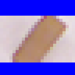
It is important for to preserve aspect ratio when feeding features into the network. This is because distorting image features may cause non-graspable rectangles to appear graspable, as shown in Fig. 5. However, padding with zeros can cause rectangles with less padding to receive higher graspability scores, as the network will have more nonzero inputs. It is important to account for this because in many cases the ideal grasp for an object might be represented by a thin rectangle which would thus contain many zero values in its receptive field from padding.

To address this problem, we scale up the magnitude of the available input for each rectangle based on the fraction of the rectangle which is masked out. In particular, we define a multiplicative scaling factor for the inputs from each modality, based on the fraction of each mode which is masked out, since each mode may have a different mask.

In the multimodal setting, we assume that the input data $x$ is known to come from $R$ distinct modalities, for example audio and video data, or depth and RGB data. We define the modality matrix $S$ as an $R$x$N$ binary matrix, where each element $S_{r,i}$ indicates membership of visible unit $x_{i}$ in a particular modality $r$, such as depth or image intensity. The scaling factor for mode $r$ is then defined as: $\Psi_{r}^{(t)}=\sum_{i=1}^{N}S_{r,i}/\left(\sum_{i=1}^{N}S_{r,i}\mu_{i}^{(t)}\right)$, where $\mu_{i}^{(t)}$ is 1 if $x_{i}^{(t)}$ is masked in, 0 otherwise. The scaling factor for case $i$ is: $\psi_{i}^{(t)}=\sum_{r=1}^{R}S_{r,i}\Psi_{r}^{(t)}$.

We could simply scale up each value of $x$ by its corresponding scale factor when training our model, as ${x^{\prime}}_{i}^{(t)}=\psi_{i}^{(t)}x_{i}^{(t)}$. However, since our sparse autoencoder penalizes squared error, scaling $x$ linearly will scale the error for the corresponding cases quadratically, causing the learning algorithm to lend increased significance to cases where more data is masked out. Instead, we can use the scaled $x^{\prime}$ as input to the network, but penalize reconstruction based on the original $x$, only scaling after the squared error has been computed:

$$W^{*} =\underset{W}{\mbox{arg min}}\sum_{t=1}^{M}\left(\sum_{i=1}^{N}\psi_{i}^{(t)}(\hat{x}_{i}^{(t)}-x_{i}^{(t)})^{2}+\lambda\sum_{j=1}^{K}g(h_{j}^{(t)})\right)$$ (5)

We redefine the hidden units to use the scaled visible input:

$$h_{j}^{(t)} =\sigma\left(\sum_{i=1}^{N}{x^{\prime}}_{i}^{(t)}W_{i,j}\right)$$ (6)

This approach is equivalent to adding additional, potentially fractional, ‘virtual’ visible units to the model based on the scaling factor for each mode. In practice, we found it necessary to limit the scaling factor to a maximum of some value $c$, as ${\Psi^{\prime}}_{r}^{(t)}=\mbox{min}(\Psi_{r}^{(t)},c)$.

As shown in Table III our mask-based scaling technique at the visible layer improves grasping results by over 25% for both metrics. As seen in Figure 6, it removes the network’s inherent bias towards square rectangles, exhibiting a much wider range of aspect ratios that more closely matches that of the ground-truth data.

V Structured Regularization for
Feature Learning

(a) Features corresponding to positive grasps.

(b) Features corresponding to negative grasps.

Figure 8: Features learned from grasping data: Each feature contains seven channels - from left to right, depth, Y, U, and V image channels, and X, Y, and Z surface normal components. Vertical edges correspond to gripper plates. Left: eight features with the strong positive correlations to rectangle graspability. Right: similar, but negative correlations. Group regularization eliminates many modalities from many of these features, making them more robust.

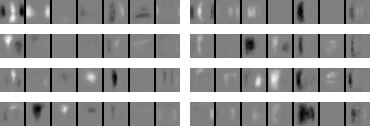
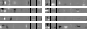
A naive way of applying feature learning to multimodal data is to simply take $x$ (as a concatenated vector) as input to the model described above, ignoring information about specific modalities, as seen on the lefthand side of Figure 7. This approach may either 1) prematurely learn features which include all modalities, which can lead to overfitting, or 2) fail to learn associations between modalities with very different underlying statistics.

Instead of concatenating multimodal input as a vector, Ngiam et al. [43] proposed training a first layer representation for each modality separately, as shown in Figure 7-middle. This approach makes the assumption that the ideal low-level features for each modality are purely unimodal, while higher-layer features are purely multimodal. This approach may work better for some problems where the modalities have very different basic representations, such as the video and audio data (as used in [43]), so that separate first layer features may give better performance. However, for modalities such as RGB-D data, where the input modes represent different channels of an image, learning low-level correlations can lead to more robust features – our experiments in Section VI show that simply concatenating the input modalities significantly outperforms training separate first-layer features for robotic grasp detection from RGB-D data.

For many problems, it may be difficult to tell which of these approaches will perform better, and time-consuming to tune and comparatively evaluate multiple algorithms. In addition, the ideal feature set for some problems may contain features which use some, but not all, of the input modalities, a case which neither of these approaches are designed to handle.

To solve these problems, we propose a new algorithm for feature learning for multimodal data. Our approach incorporates a structured penalty term into the optimization problem to be solved during learning. This technique allows the model to learn correlated features between multiple input modalities, but regularizes the number of modalities used per feature (hidden unit), discouraging the model from learning weak correlations between modalities. With this regularization term, the algorithm can specify how mode-sparse or mode-dense the features should be, representing a continuum between the two extremes outlined above.

Regularization in Deep Learning: In a typical deep learning model, $L_{2}$ regularization (i.e., $f(W)=||W||_{2}^{2}$) or $L_{1}$ regularization (i.e., $f(W)=||W||_{1}$) are commonly used in training (e.g., as specified in Equations (III-A) and (4)). These are often called a “weight cost” (or “weight decay”), and are left implicit in many works.

Applying regularization is well known to improve the generalization performance of feature learning algorithms. One might expect that a simple $L_{1}$ penalty would eliminate weak correlations in multimodal features, leading to features which use only a subset of the modes each. However, we found that in practice, a value of $\beta$ large enough to cause this also degraded the quality of features for the remaining modes and lead to decreased task performance.

Multimodal Regularization: Structured regularization, such as in [26], takes a set of groups of weights, and applies some regularization function (typically high-order) separately to each group. In our structured multimodal regularization algorithm, each modality will be used as a regularization group separately for each hidden unit. For example, a group-wise p-norm would be applied as:

$$f(W) =\sum_{j=1}^{K}\sum_{r=1}^{R}\left(\sum_{i=1}^{N}S_{r,i}|W_{i,j}^{p}|\right)^{1/p}$$ (7)

where $S_{r,i}$ is 1 if feature $i$ belongs to group $r$ and 0 otherwise. Using a high value of $p$ allows us to penalize higher-valued weights from each mode to each feature more strongly than lower-valued ones. This also means that forming a high-valued weight in a group with other high-valued weights will accrue a lower additional penalty than doing so for a group with only low-valued weights. At the limit ($p\rightarrow\infty$), this group regularization becomes equivalent to the infinity (or max) norm:

$$f(W) =\sum_{j=1}^{K}\sum_{r=1}^{R}\max_{i}S_{r,i}|W_{i,j}|$$ (8)

which penalizes only the maximum weight from each mode to each feature. In practice, the infinity norm is not differentiable and therefore is difficult to apply gradient-based optimization methods; in this paper, we use the log-sum-exponential as a differentiable approximation to the max norm.

In experiments, this regularization function produces first-layer weights concentrated in fewer modes per feature. However, we found that at values of $\beta$ sufficient to induce the desired mode-wise sparsity patterns, penalizing the maximum also had the undesirable side-effect of causing many of the weights for other modes to saturate at their mode’s maximum, suggesting that the features were overly constrained. In some cases, constraining the weights in this manner also caused the algorithm to learn duplicate (or redundant) features, in effect scaling up the feature’s contribution to reconstruction to compensate for its constrained maximum. This is obviously an undesirable effect, as it reduces the effective size (or diversity) of the learned feature set.

This suggests that the max-norm may be overly constraining. A more desirable sparsity function would penalize nonzero weight maxima for each mode for each feature without additional penalty for larger values of these maxima. We can achieve this effect by applying the $L_{0}$ norm, which takes a value of 0 for an input of 0, and 1 otherwise, on top of the max-norm from above:

$$f(W) =\sum_{j=1}^{K}\sum_{r=1}^{R}\mathbb{I}\{(\max_{i}S_{r,i}|W_{i,j}|)>0\}$$ (9)

where $\mathbb{I}$ is the indicator function, which takes a value of 1 if its argument is true, 0 otherwise. Again, for a gradient-based method, we used an approximation to the $L_{0}$ norm, such as $\log(1+x^{2})$. This regularization function now encodes a direct penalty on the number of modes used for each weight, without further constraining the weights of modes with nonzero maxima.

Figure 8 shows features learned from the unsupervised stage of our group-regularized deep learning algorithm. We discuss these features, and their implications for robotic grasping, in Section VII.

VI Experiments

Figure 9: Example objects from the Cornell grasping dataset: [28]. This dataset contains objects from a large variety of categories.

VI-A Dataset

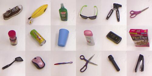
We used the extended version of the Cornell grasping dataset for our experiments. This dataset, along with code for this paper, is available at http://pr.cs.cornell.edu/deepgrasping. We note that this is an updated version of the dataset used in [28], containing several more complex objects, and thus results for their algorithms will be different from those in [28]. This dataset contains 1035 images of 280 graspable objects, several of which are shown in Fig. 9. Each image is annotated with several ground-truth positive and negative grasping rectangles. While the vast majority of possible rectangles for most objects will be non-graspable, the dataset contains roughly equal numbers of graspable and non-graspable rectangles. We will show that this is useful for an unsupervised learning algorithm, as it allows learning a good representation for graspable rectangles even from unlabeled data.

We performed five-fold cross-validation, and present results for splits on per image (i.e., the training set and the validation set do not share the same image) and per object (i.e., the training set and the validation set do not share any images from the same object) basis. Hyper-parameters were selected by validating performance on a separate set of 300 grasps not used in any of the cross-validation splits.

We take seven 24x24 pixel channels as described in Section IV as input, giving 4032 input features to each network. We trained a deep network with 200 hidden units each at the first and second layers using our learning algorithm as described in Sections III and V. Training this network took roughly 30 minutes. For trials involving our two-pass system, we trained a second network with 50 hidden units at each layer in the same manner. During inference we performed an exhaustive search using this network, then used the 200-unit network to re-rank the 100 highest-ranked rectangles found by the 50-unit network.

VI-B Baselines

We compare our recognition results in the Cornell grasping dataset with the features from [28], as well as the combination of these features and Fast Point Feature Histogram (FPFH) features [51]. We used a linear SVM for classification, which gave the best results among all other kernels. We also report chance performance, obtained by randomly selecting a label in the recognition case, and randomly assigning scores to rectangles in the detection case.

We also compare our algorithm to other deep learning approaches. We compare to a network trained only with standard L1 regularization, and a network trained in a manner similar to [43], where three separate sets of first layer features are learned for the depth channel, the combination of the Y, U, and V channels, and the combination of the X, Y, and Z surface normal components.

VI-C Metrics for Detection

For detection, we compare the top-ranked rectangle for each method with the set of ground-truth rectangles for each image. We present results using two metrics, the “point” and “rectangle” metric.

For the point metric, similar to Saxena et al. [55], we compute the center point of the predicted rectangle, and consider the grasp a success if it is within some distance from at least one ground-truth rectangle center. We note that this metric ignores grasp orientation, and therefore might overestimate the performance of an algorithm for robotic applications.

For the rectangle metric, similar to Jiang et al. [28], let $G$ be the top-ranked grasping rectangle predicted by the algorithm, and $G^{*}$ be a ground-truth rectangle. Any rectangles with an orientation error of more than $30^{o}$ from $G$ are rejected. From the remaining set, we use the common bounding box evaluation metric of intersection divided by union - i.e. $Area(G\cap G^{*})/Area(G\cup G^{*})$. Since a ground-truth rectangle can define a large space of graspable rectangles (e.g., covering the entire length of a pen), we consider a prediction to be correct if it scores at least 25% by this metric.

VII Results and Discussion

Positive
Negative

Figure 10: Learned 3D depth features: 3D meshes for depth channels of the four features with strongest positive (top) and negative(bottom) correlations to rectangle graspability. Here X and Y coordinates corresponds to positions in the deep network’s receptive field, and Z coordinates corresponds to weight values to the depth channel for each location. Feature shapes clearly correspond to graspable and non-graspable structures, respectively.

TABLE I: Recognition results for Cornell grasping dataset.

Algorithm	Accuracy (%)
Chance	50
Jiang et al. [28]	84.7
Jiang et al. [28] + FPFH	89.6
Sparse AE, separate layer-1 feat.	92.8
Sparse AE	93.7
Sparse AE, group reg.	93.7

VII-A Deep Learning for Robotic Grasp Detection

Figure 8 shows the features learned by the unsupervised phase of our algorithm which have a high correlation to positive and negative grasping cases. Many of these features show non-zero weights to the depth channel, indicating that it learns the correlation of depths to graspability. We can see that weights to many of the modalities for these features have been eliminated by our structured regularization approach. In particular, many of these features lack weights to the U and V ($3^{rd}$ and $4^{th}$) channels, which correspond to color, allowing the system to be more robust to different-colored objects.

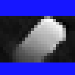
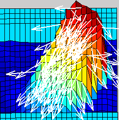
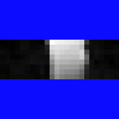
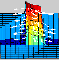
Figure 10 shows 3D meshes for the depth channels of the four features with the strongest positive and negative correlations to valid grasps. Even without any supervised information, our algorithm was able to learn several features which correlate strongly to graspable cases and non-graspable cases. The first two positive-correlated features represent handles, or other cases with a raised region in the center, while the second two represent circular rims or handles. The negatively-correlated features represent obviously non-graspable cases, such as ridges perpendicular to the gripper plane and “valleys” between the gripper plates. From these features, we can see that even during unsupervised feature learning, our approach is able to learn a representation useful for the task at hand, thanks purely to the fact that the data used is composed of half graspable and half non-graspable cases.

From Table I, we see that the recognition performance is significantly improved with deep learning methods, improving 9% over the features from [28] and 4.1% over those features combined with FPFH features. Both $L_{1}$ and group regularization performed similarly for recognition, but training separate first layer features decreased performance slightly. This shows that learned features, in addition to avoiding hand-design, are able to improve performance significantly over the state of the art. It demonstrates that a deep network is able to learn the concept of “graspability” in a way that generalizes to new objects it hasn’t seen before.

Table II shows that even using any one of the three input modalities (RGB, depth, or surface normals), our algorithm is able to learn features which outperform hand-engineered ones for recognition. Depth gives the highest performance of any single-mode network. Combining depth and normal information improves results over either alone, indicating that they give non-redundant information.

TABLE II: Recognition results for different modalities, for a deep network pre-trained using SAE.

Modes	Accuracy (%)
Chance	50
RGB	90.3
Depth	92.4
Surf. Normals	90.3
Depth + Surf. Normals	92.8
RGB + Depth + Surf. Normals	93.7

The highest accuracy is still obtained by using all the input modalities. This shows that combining depth and color information leads to a system which is more robust than either modality alone. This is due to the fact that some graspable cases (rims of monochromatic objects, etc.) can only be detected using depth information, while in others, the depth channel may be extremely noisy, requiring the use of color information. From this, we can see that integrating multimodal information, a major focus of this work, is important in recognizing good robotic grasps.

Table III shows that the performance gains from deep learning for recognition carry over to detection, as well. Once mask-based scaling has been applied, all deep learning approaches except for training separate first-layer features outperform the hand-engineered features from [28] by up to 13% for the point metric and 17% for the rectangle metric, while also avoiding the need to design task-specific features. Without mask-based scaling, the system performs poorly, due to the bias illustrated in Fig. 6. Separate first-layer features also give weak detection performance, indicating that the relative scores assigned by this form of network are less robust than those learned using our structured regularization approach.

TABLE III: Detection results for point and rectangle metrics, for various learning algorithms.

Algorithm	Image-wise split		Object-wise split
	Point	Rect	Point	Rect
Chance	35.9	6.7	35.9	6.7
Jiang et al. [28]	75.3	60.5	74.9	58.3
SAE, no mask-based scaling	62.1	39.9	56.2	35.4
SAE, separate layer-1 feat.	70.3	43.3	70.7	40.0
SAE, $L_{1}$ reg.	87.2	72.9	88.7	71.4
SAE, struct. reg., 1st pass only	86.4	70.6	85.2	64.9
SAE, struct. reg., 2nd pass only	87.5	73.8	87.6	73.2
SAE, struct. reg. two-stage	88.4	73.9	88.1	75.6

Using structured multimodal regularization also improves results over standard $L_{1}$regularization by up to 1.8%, showing that our method also learns more robust features than standard approaches which ignore modality information. Even though using the first-pass network alone underperforms the second-pass network alone by up to 8.3%, integrating both in our two-pass system outperforms the solo second-pass network by up to 2.4%. This shows that the two-pass system improves not only efficiency, but accuracy as well. The performance gains from multimodal regularization and the two-pass system are discussed in detail below.

Our system outperforms all baseline approaches by all metrics except for the point metric in the object-wise split case. However, we can see that the chance performance is much higher for the point metric than for the rectangle metric. This shows that the point metric can overstate performance, and the rectangle metric is a better indicator of the accuracy of a grasp detection system.

Wide gripper
Thin gripper
		0 degrees	45 degrees	90 degrees

Figure 11: Visualization of grasping scores for different grippers: Red indicates maximum score for a grasp with left gripper plane centered at each point, blue is similar for the right plate. Best-scoring rectangle shown in green/yellow.

Figure 12: Improvements from group regularization: Cases where our group regularization approach produces a viable grasp (shown in green and yellow), while a network trained only with simple $L_{1}$ regularization does not (shown in blue and red). Top: RGB image, bottom: depth channel. Green and blue edges correspond to gripper.

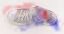
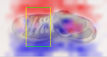
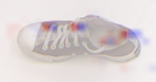
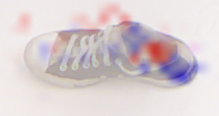
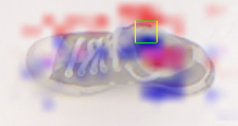
Adaptability: One important advantage of our detection system is that we can flexibly specify the constraints of the gripper in our detection system. This is particularly important for a robot like Baxter, where different objects might require different gripper settings to grasp. We can constrain the detectors to handle this. Figure 11 shows detection scores for systems constrained based on two different settings of Baxter’s gripper, one wide and one thin. The implications of these results for other types of grippers will be discussed in Section IX.

VII-B Multimodal Group Regularization

Our group regularization term improves detection accuracy over simple $L_{1}$ regularization. The improvement is more significant for the object-wise split than for the image-wise split because the group regularization helps the network to avoid overfitting, which will tend to occur more when the learning algorithm is evaluated on unseen objects.

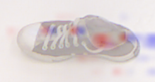
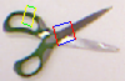
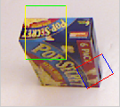
Figure 12 shows typical cases where a network trained using our group regularization finds a valid grasp, but a network trained with $L_{1}$ regularization does not. In these cases, the grasp chosen by the $L_{1}$-regularized network appears valid for some modalities – the depth channel for the sunglasses and nail polish bottle, and the RGB channels for the scissors. However, when all modalities are considered, the grasp is clearly invalid. The group-regularized network does a better job of combining information from all modalities and is more robust to noise and missing data in the depth channel, as seen in these cases.

Figure 13: Improvements from two-stage system: Example cases where the two-stage system produces a viable grasp (shown in green and yellow), while the single-stage system does not (shown in blue and red). Top: RGB image, bottom: depth channel. Green and blue edges correspond to gripper.

VII-C Two-stage Detection System

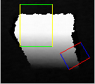
Using our two-pass system enhanced both computational performance and accuracy. The number of rectangles the full-size network needed to evaluate was reduced by roughly a factor of 1000. Meanwhile, detection performance increased by up to 2.4% as compared to a single pass with the large-size network, even though using the small network alone significantly underperforms the larger network. In most cases, the top 100 rectangles from the first pass contained the top-ranked rectangle from an exhaustive search using the second-stage network, and thus results were unaffected.

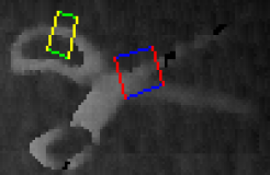
Figure 13 shows some cases where the first-stage network pruned away rectangles corresponding to weak grasps which might otherwise be chosen by the second-stage network. In these cases, the grasp chosen by the single-stage system might be feasible for a robotic gripper, but the rectangle chosen by the two-stage system represents a grasp which would clearly be successful.

The two-stage system also significantly increases the computational efficiency of our detection system. Average inference time for a MATLAB implementation of the deep network was reduced from 24.6s/image for an exhaustive search using the larger network to 13.5s/image using the two-stage system.

Figure 14: Robotic experiment objects: Several of the objects used in experiments, including challenging cases such as an oddly-shaped RC car controller, a cloth towel, plush cat, and white ice cube tray.

VIII Robotic Experiments

In order to evaluate the performance of our algorithms in the real world, we ran an extensive series of robotic experiments. To explore the generalizability and effect of the robot on the success rate of our algorithms, we performed experiments on two different robotic platforms, a Baxter Research Robot (“Yogi”) and a PR2 (“Kodiak”).

Baxter: The first platform used is our Baxter Research Robot, which we call “Yogi.” Baxter has two arms with seven degrees of freedom each and a maximum reach of 104 cm, although we used only the left arm for these experiments. The end-effector for this arm is a two-finger parallel gripper. We augmented the gripper tips using rubber bands for additional friction. Baxter’s grippers are interchangable, and we used two settings for these experiments - a “wide” setting with an open width of 8 cm and closed width of 4 cm, and a “thin” setting with an open width of 4 cm and a closed width of 0 cm (completely closed, gripper tips touching).

To detect grasps, we mounted a Kinect sensor to Yogi’s head, approximately 1.75 m above the ground. angled downwards at roughly a $75^{o}$ angle towards a table in front of it. The Kinect gives RGB-D images at a resolution of 640x480 pixels. We calibrated the transformation between the Kinect’s and Yogi’s coordinate frames by marking four points corresponding to a set of 3D axes, and obtaining the coordinates of these points in both Kinect’s and Yogi’s frames.

All control for Baxter was done by specifying an end-effector position and orientation, and using the inverse kinematics provided with Baxter to determine a set of joint angles for this pose. Baxter’s built-in control systems were used to drive the arm to these new joint angles.

PR2: Our second platform was our PR2 robot, “Kodiak.” Similar to Baxter, PR2 has two 7-DoF arms with approximately 1 m reach, and we used only the left for these experiments. PR2’s grippers open to a width of 8 cm, and are capable of closing completely from that span, so we did not need to use two settings as with Baxter. We augmented PR2’s gripper friction with gaffer tape on the fingertips.

For the experiments on PR2, we used the Kinect already mounted to Kodiak’s head, and used ROS’s built-in functionality to obtain 3D locations from that Kinect and transform these to Kodiak’s body frame for manipulation. Control was performed using the ee_cart stiffness controller [5] with trajectories provided by our own custom MATLAB code.

Experimental Setup: For each experiment, we placed a single object within a 25 cm x 25 cm square on the table, approximately 1.2 m below the mounting point of the Kinect. This square was chosen to be well-contained within each robot’s workspace, allowing objects to be reached from most approach vectors. Object positions and orientations were varied between trials, although objects were always placed in configurations in which at least one viable grasp was visible and accessible to the robot.

When using Baxter, due to the limited stroke (span from open to closed) of its gripper, we pre-selected one of the two gripper settings discussed above for each object. We constrained the search space as illustrated in Fig. 11 to find grasps for that particular setting.

To detect grasps, we first took an RGB-D image from the Kinect with no objects in the scene as a background image. The depth channel of this image was used to segment objects from the scene, and to correct for the slant of the Kinect. Once an object was segmented, we used our algorithm, as described above, to obtain a single best-ranked grasping rectangle.

The search space for the first-pass network progressed in 15-degree increments from 15 to 180 degrees (angles larger than 180 being mirror-images of grasps already tested), searching over 10-pixel increments across the image for the X and Y coordinates of the upper-left corner of the rectangle. For the thin gripper setting, rectangle widths and heights from 10 to 40 pixels in 10-pixel increments were searched, while for the thick setting these ranged from 40 pixels to 100 pixels in 20-pixel increments. In both cases, rectangles taller than they were wide were ignored. Once a single best-scoring grasp was detected, we translated it to a robotic grasp consisting of a grasping point and an approach vector using the rectangle’s parameters and the surface normal at the rectangle’s center as described above.

To execute the grasp, we first positioned the gripper at a location 10 cm back from the grasping point along the approach vector. The gripper was oriented to the approach vector, and rotated around it based on the orientation of the detected grasping rectangle.

Since Baxter’s arms are highly compliant, slight imprecisions in end-effector positioning are to be expected – we found that errors of up to 2 cm were typical. Thus, we implemented a visual servoing system using its hand camera, which provides RGB images at a resolution of 320x200 pixels. We used color segmentation to separate the object from the background, and used its lateral position in image space to drive Yogi’s end-effector to center the object. We did not implement visual servoing for PR2 because its gripper positioning was found to be precise to within 0.5 cm.

After visual servoing was completed, we drove the gripper 14 cm forwards from its current position along the approach vector, so that the grasping point was well-contained within it. We then closed the gripper, grasping the object, and moved it 30 cm upwards. A grasp was determined to be successful if it was sufficient to lift the object and hold it for one second.

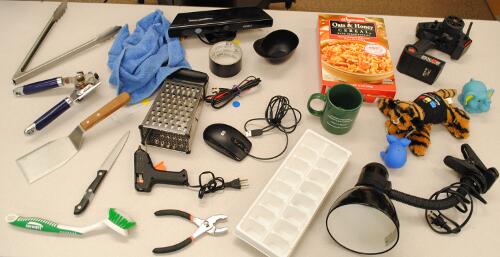
Objects to be Grasped: For our robotic experiments, we collected a diverse set of 35 objects within a size of .3 m x .3 m x .3 m and weighing at most 2.5 kg (although most were less than 1 kg) from our offices, homes, and lab. Many of them are shown in Fig. 14. Most of these objects were not present in the training dataset, and thus were completely new to the grasp detection algorithm.

Due to the physical limitations of the robots’ grippers, we found that five of these objects were not graspable even when given a hand-chosen grasp. The small pair of pliers was too low to the table to grip properly. The spray paint can was too smooth for the gripper to get enough friction to lift it. The weight of the hammer was too imbalanced, causing the hammer to rotate and slip out of the gripper when grasped. Similar problems were encountered with the bicycle U-lock. The bevel spatula’s handle was too close to the thin-set size of Baxter’s gripper, so that we could not position it precisely enough to grasp it reliably. We did not consider these objects for purposes of our experimental results, since our focus was on evaluating the performance of our grasp detection algorithm.

Results: Table LABEL:tbl:expResults shows the results of our robotic experiments on Baxter for the remaining 30 objects, a total of 100 trials. Using our algorithm, Yogi was able to successfully execute a grasp in 84% of the trials. Figure LABEL:fig:yogiGrasping shows Yogi executing several of these grasps. In 8% of the trials, our algorithm detected a valid grasp which was not executed correctly by Yogi. Thus, we were able to successfully detect a good grasp in 92% of the trials. Video of some of these trials is available at http://pr.cs.cornell.edu/deepgrasping.

PR2 yielded a higher success rate as seen in Table LABEL:tbl:pr2Results, succeeding in 89% of trials. This is largely due to the much wider span of PR2’s gripper from open to closed and its ability to fully close from its widest position, as well as PR2’s ability to apply a larger gripping force. Some specific instances where PR2 and Baxter’s performance differed are discussed below.

For comparison purposes, we ran a small set of control experiments for 16 of the objects in the dataset. The control algorithm simply returned a fixed-size rectangle centered at the object’s center of mass, as determined by depth segmentation from the background. The rectangle was aligned so that the gripper plates ran parallel to the object’s principal axis. This algorithm was only successful in 31% of cases, significantly underperforming our system.

On Baxter, our algorithm sometimes detected a grasp which was not realizable by the current setting of its gripper, but might be executable by others. For example, our algorithm detected grasps across the leg of the plush cat, and the region between the handle and body of the umbrella, both too thin for the wide setting of Baxter’s gripper to grasp since it has a minimum span of 4 cm. Since PR2’s gripper can close completely from any position, it did not encounter these issues and thus achieved a 100% success rate for both these objects.

The XBox controller proved to be a very difficult object for either robot to grasp. From a top-down angle, there is only a small space of viable grasps with a span of less than 8 cm, but many which have either a slightly larger span (making them non-realizable by either gripper), or are subtly non-viable (e.g. grasps across the two “handles,” which tend to slip off.) All viable grasps are very near to the 8 cm span of both grippers, meaning that even slight imprecision in positioning can lead to failure. Due to this, Baxter achieved a higher success rate for the XBox controller thanks to visual servoing, succeeding in 50% of cases as compared to the 25% success rate for PR2.

Our algorithm was able to consistently detect and execute valid grasps for a red cereal box, but had some failures on a white and yellow one. This is because the background for all objects in the dataset is white, leading the algorithm to learn features relating white areas at the edges of the gripper region to graspable cases. However, it was able to detect and execute correct grasps for an all-white ice cube tray, and so does not fail for all white objects. This could be remedied by extending the dataset to include cases with different background colors. Interestingly, even though the parameters of grasps detected for the white box were similar for PR2 and Baxter, PR2 was able to succeed in every case while Baxter succeeded only half the time. This is because PR2’s increased gripper strength allowed it to execute grasps across corners of the box, crushing it slightly in the process.

Other failures were due to the limitations of the Kinect sensor. We were never able to properly grasp the martini glass because its glossy finish prevented Kinect from returning any depth estimates for it. Even if a valid grasp were detected using color information only, there was no way to infer a proper grasping position without depth information. Grasps for the metal bookend failed for similar reasons, but it was not as glossy as the martini glass, and gave enough returns for some to succeed.

However, our algorithm also had many noteworthy successes. It was able to consistently detect and execute grasps for a crumpled cloth towel, a complex and irregular case which bore little resemblance to any object in the dataset. It was also able to find and grasp the rims of objects such as the plastic baseball cap and coffee mug, cases where there is little visual distinction between the rim and body of the object. These objects underscore the importance of the depth channel for robotic grasping, as none of these grasps would be detectable without depth information.

Our algorithm was also able to successfully detect and execute many grasps for which the approach vector was non-vertical. The grasps shown for the coffee mug, desk lamp, cereal box, RC car controller, and toy elephant shown in Fig. LABEL:fig:yogiGrasping were all executed by aligning the gripper to such an approach vector. Indeed, many of these grasps may have failed had the gripper been aligned vertically. This shows that our algorithm is not restricted to detecting top-down grasps, but rather encodes a more general notion of graspability which can be applied to grasps from many angles, albeit within the constraints of visibility from a single-view perspective.

While a few failures occurred, our algorithm still achieved a high rate of accuracy for other oddly-shaped objects such as the quad-rotor casing, RC car controller, and glue gun. For objects with clearly defined handles, such as the cheese grater, kitchen tongs, can opener, and knife, our algorithm was able to detect and execute successful grasps in every trial, showing that there is a wide range of objects which it can grasp extremely consistently.

IX Discussion and Future Work

Our algorithm focuses on the problem of grasp detection for a two-fingered parallel-plate style gripper. It would be directly applicable to other grippers with fixed configurations, simply requiring new training data labeled with grasps for the gripper in question. Our system would allow even the basic features used for grasp detection to adapt to the gripper. This might be useful in cases such as jamming grippers [29], or two-fingered grippers with differently-shaped contact surfaces, which might require different features to determine a graspable area.

Our detection algorithm does not directly address the problem of 3D orientation of the gripper – this orientation is determined only after an optimal rectangle has been detected, orienting the grasp based on the object’s surface normals. However, just as our approach here considers aligns a 2D feature window to the gripper, an extension of this work might align a 3D window – using voxels, rather than pixels, as its basic unit of representation for input features to the network. This would allow the system to search across the full 6-DoF 3D pose of the gripper, while still leveraging the power of feature learning.

Our system gives only a gripper pose as output, but multi-fingered reconfigurable hands also require a configuration of the fingers in order to grasp an object. In this case, our algorithm could be used as a heuristic to find one or more locations likely to be graspable (similar to the first pass in our two-pass system), greatly reducing the search space needed to find an optimal gripper configuration.

Our algorithm also depends only on local features to determine grasping locations. However, many household objects may have some areas which are strongly preferable to grasp over others - for example, a knife might be graspable by the blade, or a hot glue gun by the barrel, but both should actually be grasped by their respective handles. Since these regions are more likely to be labeled as graspable in the data, our system already weakly encodes this, but some may not be readily distinguishable using only local information. Adding a term modeling the probability of each region of the image being a semantically-appropriate area to grasp the object would allow us to incorporate this information. This term could be computed once for the entire image, then added to each local detection score, keeping detection efficient.

In this work, our visual-servoing algorithm was purely heuristic, simply attempting to center the segmented object underneath the hand camera. However, in future work, a similar feature-learning approach might be applied to hand camera images of graspable and non-graspable regions, improving the visual servoing system’s ability to fine-tune gripper position to ensure a good grasp.

Many robotics problems require the use of perceptual information, but can be difficult and time-consuming to engineer good features for, particularly when using RGB-D data. In future work, our approach could be extended to a wide range of such problems. Our system could easily be applied to other detection problems such as object detection or obstacle detection. However, it could also be adapted to other similar problems, such as object tracking and visual servoing.

Multimodal data has become extremely important for robotics, due both to the advent of new sensors such as the Kinect and the application of robots to more challenging tasks which require multiple modalities of information to perform well. However, it can be very difficult to design features which do a good job of integrating many modalities. While our work focuses on color, depth, and surface normals as input modes, our structured multimodal regularization algorithm might also be applied to others. This approach could improve performance while allowing roboticists to focus on other engineering challenges.

X Conclusions

We presented a system for detecting robotic grasps from RGB-D data using a deep learning approach. Our method has several advantages over current state-of-the-art methods. First, using deep learning allows us to avoid hand-engineering features, learning them instead. Second, our results show that deep learning methods significantly outperform even well-designed hand-engineered features from previous work.

We also presented a novel feature learning algorithm for multimodal data based on group regularization. In extensive experiments, we demonstrated that this algorithm produces better features for robotic grasp detection than existing deep learning approaches to multimodal data. Our experiments and results, both offline and on real robotic platforms, show that our two-stage deep learning system with group regularization is capable of robustly detecting grasps for a wide range of objects, even those previously unseen by the system.

References

- Bengio [2009] Y. Bengio. Learning deep architectures for AI. FTML, 2(1):1–127, 2009.
- Bicchi and Kumar [2000] A. Bicchi and V. Kumar. Robotic grasping and contact: a review. In ICRA, 2000.
- Bo et al. [2012] L. Bo, X. Ren, and D. Fox. Unsupervised Feature Learning for RGB-D Based Object Recognition. In ISER, 2012.
- Bohg et al. [accepted] J. Bohg, A. Morales, T. Asfour, and D. Kragic. Data-driven grasp synthesis - a survey. accepted.
- Bollini et al. [2011] M. Bollini, J. Barry, and D. Rus. Bakebot: Baking cookies with the pr2. In IROS PR2 Workshop, 2011.
- Bowers and Lumia [2003] D. Bowers and R. Lumia. Manipulation of unmodeled objects using intelligent grasping schemes. IEEE Trans Fuzzy Sys, 11(3), 2003.
- Cadena and Kosecka [2013] C. Cadena and J. Kosecka. Semantic parsing for priming object detection in rgb-d scenes. In ICRA Workshop on Semantic Perception, Mapping and Exploration, 2013.
- Coates and Ng [2011] A. Coates and A. Y. Ng. Selecting receptive fields in deep networks. In NIPS, 2011.
- Coates et al. [2011] A. Coates, B. Carpenter, C. Case, S. Satheesh, B. Suresh, T. Wang, D. J. Wu, and A. Y. Ng. Text detection and character recognition in scene images with unsupervised feature learning. In ICDAR, 2011.
- Collet Romea et al. [2009] A. Collet Romea, D. Berenson, S. Srinivasa, and D. Ferguson . Object recognition and full pose registration from a single image for robotic manipulation. In ICRA, 2009.
- Collet Romea et al. [2011] A. Collet Romea, M. Martinez Torres, and S. Srinivasa. The moped framework: Object recognition and pose estimation for manipulation. IJRR, 30(10):1284 – 1306, 2011.
- Collobert et al. [2011] R. Collobert, J. Weston, L. Bottou, M. Karlen, K. Kavukcuoglu, and P. Kuksa. Natural language processing (almost) from scratch. JMLR, 12:2493–2537, 2011.
- Detry et al. [2009] R. Detry, E. Baseski, M. Popovic, Y. Touati, N. Kruger, O. Kroemer, J. Peters, and J. Piater. Learning object-specific grasp affordance densities. In ICDL, 2009.
- Dogar et al. [2012] M. Dogar, K. Hsiao, M. Ciocarlie, and S. Srinivasa. Physics-based grasp planning through clutter. In RSS, 2012.
- Ekvall and Kragic [2007] S. Ekvall and D. Kragic. Learning and evaluation of the approach vector for automatic grasp generation and planning. In ICRA, 2007.
- Endres et al. [2013] F. Endres, J. Hess, J. Sturm, D. Cremers, and W. Burgard. 3d mapping with an RGB-D camera. International Journal of Robotics Research (IJRR), 2013.
- Ferrari and Canny [1992] C. Ferrari and J. Canny. Planning optimal grasps. ICRA, 1992.
- Gallegos et al. [2011] C. R. Gallegos, J. Porta, and L. Ros. Global optimization of robotic grasps. In RSS, 2011.
- Girshick et al. [2014] R. Girshick, J. Donahue, T. Darrell, and J. Malik. Rich feature hierarchies for accurate object detection and semantic segmentation. In CVPR, 2014.
- Goldfeder et al. [2009] C. Goldfeder, M. Ciocarlie, H. Dang, and P. K. Allen. The Columbia grasp database. In ICRA, 2009.
- Goodfellow et al. [2009] I. Goodfellow, Q. Le, A. Saxe, H. Lee, and A. Y. Ng. Measuring invariances in deep networks. In NIPS, 2009.
- Hinton and Salakhutdinov [2006] G. Hinton and R. Salakhutdinov. Reducing the dimensionality of data with neural networks. Science, 313(5786):504–507, 2006.
- Huebner and Kragic [2008] K. Huebner and D. Kragic. Selection of Robot Pre-Grasps using Box-Based Shape Approximation. In IROS, 2008.
- Hyvärinen et al. [2001] A. Hyvärinen, P. O. Hoyer, and M. Inki. Topographic independent component analysis. Neural computation, 13(7):1527–1558, 2001.
- Hyvärinen et al. [2002] A. Hyvärinen, J. Karhunen, and E. Oja. Principal Component Analysis and Whitening, chapter 6, pages 125–144. John Wiley & Sons, Inc., 2002.
- Jalali et al. [2010] A. Jalali, P. Ravikumar, S. Sanghavi, and C. Ruan. A dirty model for multi-task learning. In NIPS, 2010.
- Jared Glover [2008] N. R. Jared Glover, Daniela Rus. Probabilistic models of object geometry for grasp planning. In RSS, 2008.
- Jiang et al. [2011] Y. Jiang, S. Moseson, and A. Saxena. Efficient grasping from RGBD images: Learning using a new rectangle representation. In ICRA, 2011.
- Jiang et al. [2012a] Y. Jiang, J. R. Amend, H. Lipson, and A. Saxena. Learning hardware agnostic grasps for a universal jamming gripper. In ICRA, 2012a.
- Jiang et al. [2012b] Y. Jiang, M. Lim, C. Zheng, and A. Saxena. Learning to place new objects in a scene. IJRR, 31(9), 2012b.
- Kamon et al. [1996] I. Kamon, T. Flash, and S. Edelman. Learning to grasp using visual information. In ICRA, 1996.
- Kragic and Christensen [2003] D. Kragic and H. I. Christensen. Robust visual servoing. IJRR, 2003.
- Lai et al. [2011] K. Lai, L. Bo, X. Ren, and D. Fox. A large-scale hierarchical multi-view rgb-d object dataset. In ICRA, 2011.
- Lakshminarayana [1978] K. Lakshminarayana. Mechanics of form closure. ASME, 1978.
- Le et al. [2012] Q. Le, M. Ranzato, R. Monga, M. Devin, K. Chen, G. Corrado, J. Dean, and A. Ng. Building high-level features using large scale unsupervised learning. In ICML, 2012.
- Le et al. [2010] Q. V. Le, D. Kamm, A. F. Kara, and A. Y. Ng. Learning to grasp objects with multiple contact points. In ICRA, 2010.
- LeCun et al. [2004] Y. LeCun, F. Huang, and L. Bottou. Learning methods for generic object recognition with invariance to pose and lighting. In CVPR, 2004.
- Lee et al. [2009a] H. Lee, R. Grosse, R. Ranganath, and A. Y. Ng. Convolutional deep belief networks for scalable unsupervised learning of hierarchical representations. In ICML, 2009a.
- Lee et al. [2009b] H. Lee, Y. Largman, P. Pham, and A. Y. Ng. Unsupervised feature learning for audio classification using convolutional deep belief networks. In NIPS, 2009b.
- Maitin-shepard et al. [2010] J. Maitin-shepard, M. Cusumano-towner, J. Lei, and P. Abbeel. Cloth grasp point detection based on multiple-view geometric cues with application to robotic towel folding. In ICRA, 2010.
- Mohamed et al. [2012] A.-R. Mohamed, G. Dahl, and G. E. Hinton. Acoustic modeling using deep belief networks. IEEE Trans Audio, Speech, and Language Processing, 20(1):14–22, 2012.
- Morales et al. [2002] A. Morales, P. J. Sanz, and Àngel P. del Pobil. Vision-based computation of three-finger grasps on unknown planar objects. In IROS, 2002.
- Ngiam et al. [2011] J. Ngiam, A. Khosla, M. Kim, J. Nam, H. Lee, and A. Y. Ng. Multimodal deep learning. In ICML, 2011.
- Nguyen [1986] V. Nguyen. Constructing stable force-closure grasps. In ACM Fall joint computer conf, 1986.
- Osadchy et al. [2007] M. Osadchy, Y. LeCun, and M. Miller. Synergistic face detection and pose estimation with energy-based models. JMLR, 8:1197–1215, 2007.
- Papazov et al. [2012] C. Papazov, S. Haddadin, S. Parusel, K. Krieger, and D. Burschka. Rigid 3d geometry matching for grasping of known objects in cluttered scenes. IJRR, 31(4):538–553, Apr. 2012.
- Piater [2002] J. H. Piater. Learning visual features to predict hand orientations. In ICML, 2002.
- Pokorny et al. [2013] F. T. Pokorny, K. Hang, and D. Kragic. Grasp moduli spaces. In RSS, 2013.
- Ponce et al. [1993] J. Ponce, D. Stam, and B. Faverjon. On computing two-finger force-closure grasps of curved 2D objects. IJRR, 12(3):263, 1993.
- Rodriguez et al. [2011] A. Rodriguez, M. Mason, and S. Ferry. From caging to grasping. In RSS, 2011.
- Rusu et al. [2009] R. B. Rusu, N. Blodow, and M. Beetz. Fast point feature histograms (FPFH) for 3D registration. In ICRA, 2009.
- Rusu et al. [2010] R. B. Rusu, G. Bradski, R. Thibaux, and J. Hsu. Fast 3D recognition and pose using the viewpoint feature histogram. In IROS, 2010.
- Sahbani et al. [2012] A. Sahbani, S. El-Khoury, and P. Bidaud. An overview of 3d object grasp synthesis algorithms. Robot. Auton. Syst., 60(3):326–336, Mar. 2012.
- Saxena et al. [2006] A. Saxena, J. Driemeyer, J. Kearns, and A. Ng. Robotic grasping of novel objects. In NIPS, 2006.
- Saxena et al. [2008a] A. Saxena, J. Driemeyer, and A. Y. Ng. Robotic grasping of novel objects using vision. IJRR, 27(2):157–173, 2008a.
- Saxena et al. [2008b] A. Saxena, L. L. S. Wong, and A. Y. Ng. Learning grasp strategies with partial shape information. In AAAI, 2008b.
- Sermanet et al. [2013] P. Sermanet, K. Kavukcuoglu, S. Chintala, and Y. LeCun. Pedestrian detection with unsupervised multi-stage feature learning. In CVPR. 2013.
- Shimoga [1996] K. B. Shimoga. Robot grasp synthesis algorithms: A survey. IJRR, 15(3):230–266, June 1996.
- Socher et al. [2012] R. Socher, B. Huval, B. Bhat, C. D. Manning, and A. Y. Ng. Convolutional-recursive deep learning for 3D object classification. In NIPS, 2012.
- Sohn et al. [2011] K. Sohn, D. Y. Jung, H. Lee, and A. Hero III. Efficient learning of sparse, distributed, convolutional feature representations for object recognition. In ICCV, 2011.
- Srivastava and Salakhutdinov [2012] N. Srivastava and R. Salakhutdinov. Multimodal learning with deep Boltzmann machines. In NIPS, 2012.
- Szegedy et al. [2013] C. Szegedy, A. Toshev, and D. Erhan. Deep neural networks for object detection. In NIPS. 2013.
- Teuliere and Marchand [2012] C. Teuliere and E. Marchand. Direct 3d servoing using dense depth maps. In IROS, 2012.
- Viola and Jones [2001] P. Viola and M. Jones. Rapid object detection using a boosted cascade of simple features. In CVPR, 2001.
- Weisz and Allen [2012] J. Weisz and P. K. Allen. Pose error robust grasping from contact wrench space metrics. In ICRA, 2012.
- Whelan et al. [2013] T. Whelan, H. Johannsson, M. Kaess, J. Leonard, and J. McDonald. Robust real-time visual odometry for dense RGB-D mapping. In ICRA, 2013.
- Zhang et al. [2011] L. Zhang, M. Ciocarlie, and K. Hsiao. Grasp evaluation with graspable feature matching. In RSS Workshop on Mobile Manipulation, 2011.