Impact of the non-Gaussian covariance of the weak lensing power spectrum and bispectrum on cosmological parameter estimation

Abstract

We study how well the Gaussian approximation is valid for computing the covariance matrices of the convergence power and bispectrum in weak gravitational lensing analyses. We focus on its impact on the cosmological parameter estimations by comparing the results with and without non-Gaussian error contribution in the covariance matrix. We numerically derive the covariance matrix as well as the cosmology dependence of the spectra from a large set of $N$-body simulations performed for various cosmologies and carry out Fisher matrix forecasts for tomographic weak lensing surveys with three source redshifts. After showing the consistency of the power and bispectra measured from our simulations with the state-of-the-art fitting formulas, we investigate the covariance matrix assuming a typical ongoing survey across 1500 deg² with the mean source number density of 30 arcmin^-2 at the mean redshift $z_{s}=1.0$. Although the shape noise contributes a significant fraction to the total error budget and it mitigates the impact of the non-Gaussian error for this source number density, we find that the non-Gaussian error degrades the cumulative signal-to-noise ratio up to the maximum multipole of 2000 by a factor of about 2 (3) in the power (bi-) spectrum analysis. Its impact on the final cosmological parameter forecast with $6$ parameters can be as large as $15\%$ in the size of the one-dimensional statistical error. This can be a problem in future wide and deep weak lensing surveys for precision cosmology. We also show how much the dark energy figure of merit is affected by the non-Gaussian error contribution and demonstrate an optimal survey design with a fixed observational time.

I Introduction

Cosmological weak gravitational lensing has been becoming the focus of attention as a powerful tool to probe the distribution of the matter in the Universe, since its first detections (Bacon et al., 2000; Kaiser et al., 2000; Van Waerbeke et al., 2000; Wittman et al., 2000). Light rays from distant galaxies are bent by the gravitational potential of intervening large scale structures, which generate coherent deformation of galaxy images and this is the so-called cosmic shear. We can directly see the distribution of matter, and measure the statistical quantities such as the power spectrum and bispectrum of mass fluctuations on cosmological scales by analyzing this coherent pattern.

Weak lensing can also be a powerful probe of the nature of dark energy. The growth rate of mass clustering can be measured by lensing tomography (e.g., Hu, 1999; Huterer, 2002; Takada and Jain, 2004) which in turn provides tight constraints on the equation of state of dark energy. For this purpose, a number of ambitious wide-field surveys have been proposed, such as Subaru Hyper Suprime-Cam Survey (HSC)  (Miyazaki et al., 2006), the Dark Energy Survey (DES)  (The Dark Energy Survey Collaboration, 2005), the Large Synoptic Survey Telescope (LSST)  (LSST Science Collaborations et al., 2009), the Wide-Field Infrared Survey Telescope (WFIRST), and Euclid (Laureijs et al., 2011).

Unlike the cosmic microwave background, the distribution of matter in the present Universe which determines the weak lensing convergence field is highly nonlinear and non-Gaussian, reflecting the nonlinear processes that accompanied structure formation (Taruya et al., 2002; Sato et al., 2011a; Seo et al., 2011; Takahashi et al., 2011). Thus, some of the cosmological information initially stored in the two-point correlation function and/or the power spectrum when the density field was in the linear stage is no longer present in two-point statistics of the nonlinear convergence field. If we want to draw as much information as possible from the convergence field, it is of great importance to add the information contained in the higher-order statistics such as the bispectrum on top of the two-point statistics or to resort to alternative nonstandard methods.

Recently, it was suggested that the two-point statistics of the logarithmic transformed nonlinear weak lensing field may contain more information than the two-point statistics of the original field before transformation (e.g., Seo et al., 2011). Seo et al. (2011) showed that, by Taylor expanding the log-transformed field, most of the improvement by the transformation can be explained by the information originally contained in the bispectrum, suggesting that the log transform is a way to draw some information in the higher-order statistics back to the two-point statistics. However, it was also shown that the log transform is advantageous when one is interested in a single parameter such as the amplitude of the power spectrum. Seo et al. (2012) found that there is only little improvement in the constraints on multiple cosmological parameters after log transform in the presence of shape noise that are expected from future weak lensing surveys.

We therefore focus on the weak lensing bispectrum itself as a higher-order statistic in this study. We study the usefulness and complementarity of the lensing bispectrum compared to the power spectrum using 1000 ray-tracing weak lensing maps generated in Seo et al. (2012). We consider all the possible triangular configurations available from a given range of multipoles and examine the impact of the bispectrum on cosmological parameter estimation taking non-Gaussian covariance matrices obtained from ray-tracing simulations into account. In doing this, we perform a Fisher matrix analysis of a tomographic survey with three different source redshifts using the fully non-Gaussian covariance matrix and derivatives of the spectra with respect to the cosmological parameters directly measured from the simulations.

The paper of Kayo et al. (2013) that recently appeared is based on a similar analysis. They mainly focused on the covariance matrix itself and examined the impact of the new contribution coming from the number fluctuation of massive halos in a finite survey area based on halo model (Sato et al., 2009), which we hereafter refer to as halo sample variance (HSV). In this paper, we will extend their analysis to the information content of the power and the bispectrum tomography in terms of the cosmological parameter constraints.

This paper is organized as follows. In Section II, we briefly review the basic theoretical expectations of the lensing power and bispectrum and their covariances. We describe the details of our $N$-body simulations used in this paper and data analysis in Section III. In Section IV, we present the detailed comparisons between the simulation results and previous models for the weak lensing power and bispectrum. After studying the bispectrum covariance using the simulations in Section V, we study cumulative signal-to-noise ratio of the power spectra, bispectra and the joint measurement of them in Section VI. In Section VII, we present how significant the non-Gaussian errors of the weak lensing power and bispectrum are in constraining the cosmological parameters by using the Fisher matrix analysis. In Section VIII, we examine the dark energy figure of merit (FoM) in the presence of the non-Gaussian corrections to the covariance matrix, and demonstrate an optimal survey design by changing the mean number density of source galaxies and the survey area under the condition that the total observation time is fixed. Finally, Section IX is devoted to conclusion and discussion.

II Preliminaries

II.1 Lensing power spectrum and bispectrum

In this paper, we consider an ideal source galaxy distribution where all of them are located at a single redshift when we compare with simulations. By using the Born approximation, the weak lensing convergence field can be written as a weighted projection of the three-dimensional density contrast (e.g., Bartelmann and Schneider, 2001; Munshi et al., 2008)

$$\kappa(\bm{\theta})=\int_{0}^{\chi_{s}}{\rm d}\chi\,W(\chi)\delta(\chi,f_{K}(\chi)\bm{\theta}),$$ (1)

where $\bm{\theta}$ is the two-dimensional vector denoting the angular position on the sky, $\chi$ is the comoving distance, $\chi_{s}$ is the comoving distance to the source, $f_{K}(\chi)$ is the comoving angular diameter distance, and $W(\chi)$ is the lensing weight function defined as

$$W(\chi;z)=\frac{3\Omega_{\rm m}H_{0}^{2}f_{K}(\chi)f_{K}(\chi_{s}-\chi)}{2c^{2}f_{K}(\chi_{s})}(1+z).$$ (2)

To compute the power and bispectrum of the convergence, we employ the flat-sky approximation which is sufficiently accurate over angular scales of our interest. Within this approximation, the lensing convergence field is decomposed into angular modes based on two-dimensional Fourier transform:

$$\kappa(\bm{\theta})=\int\frac{{\rm d}^{2}\bm{l}}{(2\pi)^{2}}\,e^{i\bm{l}\cdot\bm{\theta}}\tilde{\kappa}(\bm{l}).$$ (3)

For a two-dimensional homogeneous and isotropic random field, one can define the convergence power spectrum and bispectrum as

$$\langle\tilde{\kappa}(\bm{l}_{1})\tilde{\kappa}(\bm{l}_{2})\rangle=(2\pi)^{2}\delta_{D}(\bm{l}_{1}+\bm{l}_{2})P_{\kappa}(l_{1}),$$ (4)

and

$$\langle\tilde{\kappa}(\bm{l}_{1})\tilde{\kappa}(\bm{l}_{2})\tilde{\kappa}(\bm{l}_{3})\rangle=(2\pi)^{2}\delta_{D}(\bm{l}_{1}+\bm{l}_{2}+\bm{l}_{3})B_{\kappa}(l_{1},l_{2},l_{3}),$$ (5)

where $\delta_{D}(\bm{l})$ is the Dirac delta function. By using the Limber approximation (Limber, 1954; Kaiser, 1992), the convergence power spectrum and bispectrum are given by (e.g., Bartelmann and Schneider, 2001; Munshi et al., 2008)

$$P_{\kappa}(l)=\int_{0}^{\chi_{s}}{\rm d}\chi\,\frac{W(\chi)^{2}}{f_{K}(\chi)^{2}}\,P_{\delta}\left(k=\frac{l}{f_{K}(\chi)};z\right),$$ (6)

$$B_{\kappa}(\bm{l}_{1},\bm{l}_{2},\bm{l}_{3})=\int_{0}^{\chi_{s}}{\rm d}\chi\,\frac{W(\chi)^{3}}{f_{K}(\chi)^{4}}\,B_{\delta}(\bm{k}_{1},\bm{k}_{2},\bm{k}_{3};z),$$ (7)

where $\bm{k}_{i}=\bm{l}_{i}/f_{K}(\chi)$, $P_{\delta}(k;z)$, and $B_{\delta}(\bm{k}_{1},\bm{k}_{2},\bm{k}_{3};z)$ are the three-dimensional power spectrum and bispectrum of the matter density contrast at redshift $z$. The nonlinear gravitational evolution of $P_{\delta}$ and $B_{\delta}$ significantly enhances the amplitude of the lensing power and bispectrum respectively at $l\lower 2.15277pt\hbox{$\;\buildrel>\over{\sim}\;$}100$ for source redshift $z_{s}=1.0$ (see Figures 1 and 2). Therefore, we need to take nonlinear evolution effect into account for weak lensing studies. We employ some fitting formulas for the three-dimensional spectra in analytically evaluating the convergence spectra; halofit proposed by Smith et al. (2003) and a refined version of that proposed by Takahashi et al. (2012) (hereafter revised halofit) for $P_{\delta}$ and Scoccimarro and Couchman (2001) (hereafter SC01) and Gil-Marín et al. (2012) (hereafter Gil-Marin12) for $B_{\delta}$ in Section IV. The two fitting functions for the bispectrum explicitly include $P_{\delta}$, and we will use halofit and revised halofit for that.

II.2 Covariance matrices of the lensing power spectrum and bispectrum

The covariance matrix of the convergence power spectrum between $P_{\kappa}(l)$ and $P_{\kappa}(l^{\prime})$ can be expressed as a sum of the Gaussian and non-Gaussian contributions (Cooray and Hu, 2001; Sato et al., 2009):

$${\rm Cov} [P_{\kappa}(l),P_{\kappa}(l^{\prime})]=\frac{2}{N_{l}}P_{\kappa}(l)^{2}\delta^{K}_{l,l^{\prime}}$$

$$+\frac{1}{\Omega_{\rm s}}\int_{l_{1}\in l}\frac{{\rm d}^{2}\bm{l_{1}}}{A_{\rm s}(l)}\int_{l_{1}^{\prime}\in l^{\prime}}\frac{{\rm d}^{2}\bm{l_{1}^{\prime}}}{A_{\rm s^{\prime}}(l^{\prime})}T_{\kappa}(\bm{l_{1}},-\bm{l_{1}},\bm{l_{1}^{\prime}},-\bm{l_{1}^{\prime}}),$$ (8)

where $\delta^{K}_{l,l^{\prime}}$ is the Kronecker delta function, $\Omega_{\rm s}$ is the survey area, and $T_{\kappa}$ is the lensing trispectrum defined as

$$\langle\tilde{\kappa}(\bm{l}_{1})\tilde{\kappa}(\bm{l}_{2})\tilde{\kappa}(\bm{l}_{3})\tilde{\kappa}(\bm{l}_{4})\rangle\equiv(2\pi)^{2}\delta_{D}(\bm{l}_{1234})T_{\kappa}(\bm{l}_{1},\bm{l}_{2},\bm{l}_{3},\bm{l}_{4}),$$ (9)

where we have introduced a shorthand notation $\bm{l}_{1234}=\bm{l}_{1}+\bm{l}_{2}+\bm{l}_{3}+\bm{l}_{4}$. In the above, $N_{l}$ denotes the number of modes around a bin labeled by $l$ and is approximately given by $N_{l}=A_{\rm s}\Omega_{\rm s}/(2\pi)^{2}$ with $A_{\rm s}=2\pi l\Delta l$ being the area of the two-dimensional shell around that bin. Therefore, $l$ denotes the mean radius of the annulus. In the Limber approximation, $T_{\kappa}$ is simply a projection of the three-dimensional mass trispectrum $T_{\delta}$ given by

$$T_{\kappa}(\bm{l}_{1},\bm{l}_{2},\bm{l}_{3},\bm{l}_{4})=\int_{0}^{\chi_{s}}{\rm d}\chi\frac{W(\chi)^{4}}{f_{K}(\chi)^{6}}T_{\delta}\left(\bm{k}_{1},\bm{k}_{2},\bm{k}_{3},\bm{k}_{4};z\right).$$ (10)

However, there is an additional contribution to the non-Gaussian covariance, which becomes significant on small scales. This additional variance, HSV, is expressed as (Sato et al., 2009)

$${\rm Cov}_{{\rm HSV}}[P_{\kappa}(l),P_{\kappa}(l^{\prime})]=\int_{0}^{\chi_{s}}{\rm d}\chi\left(\frac{{\rm d}^{2}V}{{\rm d}\chi{\rm d}\Omega}\right)^{2}$$

$$\times\int{\rm d}M\frac{{\rm d}n}{{\rm d}M}b(M)|\tilde{\kappa}_{M}(l)|^{2}\int{\rm d}M^{\prime}\frac{{\rm d}n}{{\rm d}M^{\prime}}b(M^{\prime})|\tilde{\kappa}_{M^{\prime}}(l^{\prime})|^{2}$$

$$\times\int\frac{k{\rm d}k}{2\pi}\!P_{\delta}^{\rm L}(k;z)\left|\widetilde{W}\!\left(k\chi\Theta_{\rm s}\right)\right|^{2},$$ (11)

where ${\rm d}^{2}V/{\rm d}\chi{\rm d}\Omega$ is the comoving volume per unit radial comoving distance and unit solid angle, and is given by $\chi^{2}$ for a flat universe, ${\rm d}n/{\rm d}M$ is the ensemble-averaged halo mass function, $b(M)$ is the halo bias parameter, and $\tilde{\kappa}_{M}(l)$ is the angular Fourier transform of the convergence field generated by the density profile of a halo with mass $M$. Also, $\widetilde{W}(x)$ is the Fourier transform of the survey window function and $\Theta_{\rm s}$ is the radius of survey geometry. It should be noted that HSV contribution does not necessarily scale with $1/\Omega_{\rm s}$ unlike other covariance terms because the sample variance depends on $\Omega_{\rm s}$ via the shape of the linear power spectrum $P_{\delta}^{\rm L}(k)$. The contribution of Equation (11) arises for any finite-volume survey because the halo distribution has modulations due to the biased density fluctuations over the survey window.

Meanwhile, the covariance matrix of the convergence bispectrum is defined as a sum of five terms (Joachimi et al., 2009; Kayo et al., 2013):

$${\rm Cov}[B_{\kappa}(l_{1},l_{2},l_{3}), B_{\kappa}(l_{1}^{\prime},l_{2}^{\prime},l_{3}^{\prime})]=\gamma P_{\kappa}(l_{1})P_{\kappa}(l_{2})P_{\kappa}(l_{3})$$

$$+T_{3\times 3}+T_{4\times 2}+T_{6}+{\rm Cov}_{\rm HSV}^{\rm BB}.$$ (12)

The first term is proportional to the triple product of the lensing power spectrum with an amplitude given by the geometrical factor:

$$\gamma=\frac{(2\pi)^{3}D_{l_{1},l_{2},l_{3},l_{1}^{\prime},l_{2}^{\prime},l_{3}^{\prime}}}{\Omega_{\rm s}l_{1}l_{2}l_{3}\Delta{l_{1}}\Delta{l_{2}}\Delta{l_{3}}}\Lambda^{-1}(l_{1},l_{2},l_{3}),$$ (13)

where

$$D_{l_{1},l_{2},l_{3},l_{1}^{\prime},l_{2}^{\prime},l_{3}^{\prime}} =\delta^{K}_{l_{1},l_{1}^{\prime}}\delta^{K}_{l_{2},l_{2}^{\prime}}\delta^{K}_{l_{3},l_{3}^{\prime}}+\delta^{K}_{l_{1},l_{2}^{\prime}}\delta^{K}_{l_{2},l_{1}^{\prime}}\delta^{K}_{l_{3},l_{3}^{\prime}}$$

$$+\delta^{K}_{l_{1},l_{1}^{\prime}}\delta^{K}_{l_{2},l_{3}^{\prime}}\delta^{K}_{l_{3},l_{2}^{\prime}}+\delta^{K}_{l_{1},l_{2}^{\prime}}\delta^{K}_{l_{2},l_{3}^{\prime}}\delta^{K}_{l_{3},l_{1}^{\prime}}$$

$$+\delta^{K}_{l_{1},l_{3}^{\prime}}\delta^{K}_{l_{2},l_{1}^{\prime}}\delta^{K}_{l_{3},l_{2}^{\prime}}+\delta^{K}_{l_{1},l_{3}^{\prime}}\delta^{K}_{l_{2},l_{2}^{\prime}}\delta^{K}_{l_{3},l_{1}^{\prime}},$$ (14)

and

$$\Lambda^{-1}(l_{1},l_{2},l_{3})=\frac{1}{4}\sqrt{2l_{1}^{2}l_{2}^{2}+2l_{1}^{2}l_{3}^{2}+2l_{2}^{2}l_{3}^{2}-l_{1}^{4}-l_{2}^{4}-l_{3}^{4}},$$ (15)

if $|l_{1}-l_{2}|<l_{3}<l_{1}+l_{2}$ and permutations thereof are satisfied, else $\Lambda^{-1}(l_{1},l_{2},l_{3})=0$. This factor shows the area of a triangle with side lengths $l_{1}$, $l_{2}$, and $l_{3}$. We refer to the first term of Equation (12) as the Gaussian contribution, while the other four terms denote the non-Gaussian contributions that arise from the connected three-, four-, six-point function of the convergence field, and the number fluctuations of massive halos in a finite survey area (see (Kayo et al., 2013) for the exact expressions), while (Joachimi et al., 2009) missed the final term which is dominant over the other covariance term at $l\lower 2.15277pt\hbox{$\;\buildrel>\over{\sim}\;$}1000$ even if survey area is a few thousand (see Figure 2 in Kayo et al. (2013)).

Only the first term in Equation (12) is usually discussed in previous statistical analyses of the cosmological fields in the literature Takada and Jain (2004); Martin et al. (2012) except for Kayo et al. (2013), just because of simplicity and/or difficulty of calculation of the last four terms (see (e.g., Kilbinger and Schneider, 2005; Semboloni et al., 2011) for real-space analyses of third-order lensing measurements). We will carefully examine how well the approximation of Gaussianity (here, the word “Gaussianity” means that the covariance matrix of the power spectrum and bispectrum is described by only the first term of Equations 8 and 12) is valid for computing the bispectrum covariance and its impact on cosmological parameter estimations, by comparing with the fully nonlinear covariance matrix measured from a large ensemble of ray-tracing simulations.

III Numerical Simulation

III.1 Simulation design

In order to study the impact of the non-Gaussian error of the convergence power and bispectrum on cosmological parameter estimations, we perform a large set of ray-tracing simulations through large-volume, high-resolution $N$-body simulations of structure formation (Jain et al., 2000; Hamana and Mellier, 2001; Hilbert et al., 2009; Sato et al., 2009). We use a modified version of the Gadget-2 code (Springel, 2005) for the $N$-body simulations. The matter density fields in quasilight cone volumes are constructed by combining $2\times 200$ realizations of $N$-body simulations performed in cubes with 240 and 480$h^{-1}$Mpc on a side, and we perform ray-tracing simulations through these volumes. We employ 256³ particles for each $N$-body simulation. For our fiducial cosmology, we adopt the standard $\Lambda$CDM model with density parameter of matter $\Omega_{\rm m}=0.238$, baryon $\Omega_{\rm b}=0.0416$, and dark energy $\Omega_{\Lambda}=0.762$ with the current value of the equation of state parameter $w_{0}=-1$ and its time evolution $w_{a}=0$, the primordial spectrum with the spectral index $n_{s}=0.958$ and the normalization $A_{\rm s}=2.35\times 10^{-9}$, and the Hubble parameter $h=0.732$, which are consistent with the WMAP 3-year results (Spergel et al., 2007). The amplitude of the linear density fluctuations in a sphere of radius 8$h^{-1}$Mpc at present time is $\sigma_{8}=0.759$ in this cosmology. We assume three delta-function-like source redshifts at $z_{s}=0.6$, 1.0, and 1.5 to perform a tomographic study. Using ray-tracing simulations we generate 1000 realizations of 5${}^{\circ}\times 5^{\circ}$ convergence maps for each of the three source redshifts. It was shown that the ray-tracing simulations are reliable within a 5% accuracy up to $l\sim 6000$ and $l\sim 4000$ at $z_{s}=1.0$ in terms of the power spectrum and the bispectrum, respectively (see Sato et al., 2009; Valageas et al., 2012a).

In addition to the fiducial cosmology, we also perform ray-tracing simulations for several cosmologies with slightly different parameters. We vary each of the following cosmological parameters: $A_{s}$, $n_{s}$, the cold dark matter density $\Omega_{\rm c}h^{2}$, $\Omega_{\Lambda}$, and $w_{0}$ by $\pm 10\%$, and $w_{a}$ by $\pm$0.5. In varying the parameters, we keep the flatness of the Universe as well as the physical baryon density $\Omega_{\rm b}h^{2}$ unchanged. Therefore, the three parameters, $h$, $\Omega_{\rm m}$, and $\Omega_{\rm b}$, are varied simultaneously to satisfy the above condition. For each of these 12 different cosmologies, we generate 40 realizations of convergence fields for each of the three source redshifts. See Sato et al. (2009) for more details of the methods used for the ray-tracing simulations (see also Sato et al. (2011a)). All the convergence maps used in this paper are the same as those used in Seo et al. (2012).

We include only the auto spectra in our tomographic analysis. We assume a future, wide-field weak lensing survey of 1500 deg², expected for Subaru HSC Weak Lensing Survey (Miyazaki et al., 2006) for the signal-to-noise ratio and the Fisher matrix analyses presented below. We simply scale each element of the covariance matrix obtained from ray-tracing simulations by the ratio of the area, 1/(1500/25), although strictly speaking, the HSV terms have a different scaling. The inaccuracy of the above scaling is shown to have little impact on the estimation of signal-to-noise ratio (see the left panel of Figure 11 in Kayo et al. (2013)). For cosmological parameter constraints, this difference is much smaller than the signal-to-noise ratio as discussed in Section IX. Therefore, we use this simple scaling for the covariance matrix, which does not change the results quantitatively.

In reality, the observed power spectrum is contaminated by the intrinsic ellipticity noise. For the simulated convergence map, we can include the noise contamination by adding, to each pixel, a random Gaussian distributed noise with variance

$$\sigma_{N}^{2}=\frac{\sigma_{\gamma}^{2}}{\bar{n}_{g}\Omega_{\rm pix}}=\frac{1}{\bar{n}_{g}\Omega_{\rm pix}}\left(\frac{\sigma_{\rm int}}{\mathcal{R}}\right)^{2},$$ (16)

where $\sigma_{\gamma}$ is the rms of the intrinsic shear, $\bar{n}_{g}$ is the mean number density of source galaxies, and $\Omega_{\rm pix}$ is the pixel area. Here, we set the intrinsic shape noise as $\sigma_{\rm int}=0.374$ and the shear responsivity as $\mathcal{R}=1.7$ (Mandelbaum et al., 2006). We also adopt $\bar{n}_{g}=12.75$, 7.91, and 9.0 arcmin^-2 at three source redshifts, $z_{s}=0.6$, 1.0, and 1.5, respectively. These values are roughly expected in Subaru Hyper Suprime-Cam Weak Lensing Survey (Miyazaki et al., 2006) and calculated from Equation (20) in Takada and Jain (2009), by dividing source galaxies into $0<z_{s}<0.8$, $0.8\leq z_{s}<1.2$, and $1.2\leq z_{s}$.

III.2 Analysis

The binned power and bispectrum of the convergence field are measured from the simulations as follows. We first apply fast Fourier transformation to each of the convergence fields to obtain $\tilde{\kappa}(\bm{l})$. We then bin the data into logarithmically equal bins in $l$, whose width are set as $\Delta\ln l=\ln 2/2\approx 0.35$. The power spectrum and the bispectrum of the $m$th realization are obtained by simply averaging the products of modes:

$$\hat{P}_{\kappa}^{m}(l) =\frac{1}{N_{l}}\sum_{|\bm{l}|\in l}|\tilde{\kappa}(\bm{l})|^{2},$$ (17)

$$\hat{B}_{\kappa}^{m}(\bm{l}_{1},\bm{l}_{2},\bm{l}_{3}) =\frac{1}{N_{l_{1},l_{2},l_{3}}}\sum_{|\bm{l}_{i}|\in l_{i}}{\rm Re}\left[\tilde{\kappa}(\bm{l}_{1})\tilde{\kappa}(\bm{l}_{2})\tilde{\kappa}(\bm{l}_{3})\right],$$ (18)

where Re[…] denotes the real part of a complex number, and the summation runs over modes $\bm{l}$ ($\bm{l}_{i}$, $i=1,2,3$) which falls into bin $l$ ($l_{i}$) for the power (bi-) spectrum. In the above, $N_{l}$ is the number of modes taken for the summation. Similarly, the factor $N_{l_{1},l_{2},l_{3}}$, which appears in the estimator of the bispectrum, denotes the number of triangles in $l$ space. We then average the measured spectra over 1000 random realizations to obtain our final estimates of $P_{\kappa}$ and $B_{\kappa}$. We also estimate the the full covariance matrix of the power and bispectrum including not only the covariance between two different bins inside each of the two spectra, but also their cross covariance using the 1000 realizations as follows:

$${\rm Cov}\left[P_{\kappa}(l),P_{\kappa}(l^{\prime})\right] =\frac{1}{N_{R}-1}\sum_{m=1}^{N_{R}}\left(\hat{P}_{\kappa}^{m}(l)-P_{\kappa}(l)\right)\left(\hat{P}_{\kappa}^{m}(l^{\prime})-P_{\kappa}(l^{\prime})\right),$$ (19)

$${\rm Cov}\left[B_{\kappa}(\bm{l}_{1},\bm{l}_{2},\bm{l}_{3}),B_{\kappa}(\bm{l}_{1}^{\prime},\bm{l}_{2}^{\prime},\bm{l}_{3}^{\prime})\right] =\frac{1}{N_{R}-1}\sum_{m=1}^{N_{R}}\left(\hat{B}_{\kappa}^{m}(\bm{l}_{1},\bm{l}_{2},\bm{l}_{3})-B_{\kappa}(\bm{l}_{1},\bm{l}_{2},\bm{l}_{3})\right)\left(\hat{B}_{\kappa}^{m}(\bm{l}_{1}^{\prime},\bm{l}_{2}^{\prime},\bm{l}_{3}^{\prime})-B_{\kappa}(\bm{l}_{1}^{\prime},\bm{l}_{2}^{\prime},\bm{l}_{3}^{\prime})\right),$$ (20)

$${\rm Cov}\left[P_{\kappa}(l),B_{\kappa}(\bm{l}_{1},\bm{l}_{2},\bm{l}_{3})\right] =\frac{1}{N_{R}-1}\sum_{m=1}^{N_{R}}\left(\hat{P}_{\kappa}^{m}(l)-P_{\kappa}(l)\right)\left(\hat{B}_{\kappa}^{m}(\bm{l}_{1},\bm{l}_{2},\bm{l}_{3})-B_{\kappa}(\bm{l}_{1},\bm{l}_{2},\bm{l}_{3})\right),$$ (21)

where $N_{R}$ is number of realizations. Note that these are unbiased maximum-likelihood estimators for the covariance matrices.

IV Comparison of fitting formulas with ray-tracing simulations

We now compare the convergence power and bispectra measured from our ray-tracing simulation with fitting models, which have been used in some previous works.

IV.1 Weak lensing power spectrum

Figure 1: Convergence power spectrum at source redshifts $z_{s}=1.0$. The cross symbols are the results of the ray-tracing simulations with 1-$\sigma$ error bars assuming the survey area of $\Omega_{\rm s}=1500$ deg². The solid and dashed lines show the two fitting formulas, revised halofit and halofit, respectively. We also show the linear theory prediction by a long-dashed line. The vertical arrow denotes the multipole $l$ up to which the ray-tracing simulation result is accurate within 5%, which is determined based on a convergence test using higher resolution simulations.

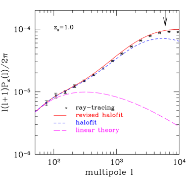
Figure 1 shows the convergence power spectrum obtained from ray-tracing simulations with 1-$\sigma$ error bars expected from a HSC-type survey, i.e., $\Omega_{\rm s}=1500$ deg² for $z_{s}=1.0$. The numerical error bars increase on large scales because of the finite size of the simulation box. We compare the simulation result with two fitting formulas for the matter power spectrum, revised halofit (solid line) and halofit (dashed line). For reference we also plot the linear power spectrum result as a long-dashed line. The vertical arrow indicates the multipole below which the simulation result is consistent with higher-resolution simulations (512³particles) within 5%.

The nonlinear gravitational evolution of the matter density field amplifies the weak lensing power spectrum on small scales. We recover a well-known fact that the halofit underpredicts the convergence power on small scales $l\lower 2.15277pt\hbox{$\;\buildrel>\over{\sim}\;$}3000$ (e.g., Hilbert et al., 2009; Sato et al., 2009; Valageas et al., 2012a; Becker, 2012), while the revised halofit shows a better match to the simulations. This consistency with independent simulations in the literature assures the reliability of our simulations.

Another option to obtain an accurate prediction of the power spectrum over a wide range in multipole $l$ is to use the model combining perturbation theories at small $l$ and halo model at large $l$, proposed by Valageas and Nishimichi (2011) (hereafter combined theory). However, it is not straightforward to calculate the combined theory, especially its 2-halo term, because it involves some renormalization techniques with time-consuming multidimensional integrals. We thus adopt the fitting formulas in this paper for simplicity, but see Valageas et al. (2012a, b) for an extensive comparisons with this combined theory with the same numerical simulations as presented in this paper.

IV.2 Weak lensing bispectra for equilateral triangles

Figure 2: Left and right panels show the convergence bispectrum and reduced bispectrum at source redshift $z_{s}=1.0$ for equilateral triangles. The solid and dashed curves are the results of Scoccimarro and Couchman (2001) fitting formula, while the dot-dashed and dotted curves are those of Gil-Marín et al. (2012) fitting formula with the revised halofit and original halofit, respectively. The tree-level perturbation theory prediction is plotted as long-dashed lines. The vertical arrow shows the scale up to which the ray-tracing result is valid within 5%.

Figure 3: The reduced bispectrum as a function of $l_{1}=l_{2}$ at source redshift $z_{s}=1.0$ for isosceles configurations, where $l_{3}$ is chosen to 152 (left panel), 431 (middle panel), and 1,218 (right panel). The solid and dot-dashed lines are the results of Scoccimarro and Couchman (2001) and Gil-Marín et al. (2012) fitting formula with the revised halofit.

Figure 4: The reduced bispectrum as a function of $l_{3}$ at source redshift $z_{s}=1.0$ for isosceles configurations, where $l_{1}=l_{2}$ is chosen to 431 (left panel), 1,218 (middle panel), and 3,444 (right panel). The symbols and lines are the same as the Figure 3.

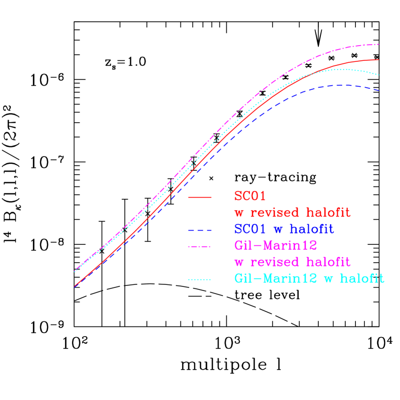
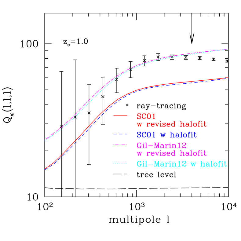
Left panel in Figure 2 shows the convergence bispectrum measured from the 1000 ray-tracing simulations at source redshift $z_{s}=1.0$ for equilateral triangles. We compare it with several fitting formulas to check the validity and usefulness of them. The error bars are expected errors for $\Omega_{\rm s}=1500$ deg² as before. Theoretical predictions are calculated from Equation (7) using the fitting formulas proposed by SC01 or Gil-Marin12 for $B_{\delta}$. The solid and dashed curves show the SC01 fitting formula, while the dot-dashed and dotted curves are the Gil-Marin12 fitting formula with revised halofit and original halofit, respectively. We also plot the tree-level perturbation theory (Bernardeau et al., 2002) in long-dashed lines. It is shown that nonlinear gravitational clustering significantly enhances the bispectrum amplitude compared to the tree-level perturbation theory prediction by more than an order of magnitude at $l\lower 2.15277pt\hbox{$\;\buildrel>\over{\sim}\;$}500$. The vertical arrow at $l\sim 4000$ shows the multipole $l$ up to which the ray-tracing simulation result is valid within 5% for the bispectrum (see Valageas et al., 2012a).

From this figure, it is not obvious to conclude which fitting formula gives a better prediction, because the power spectrum in evaluating the fitting formula of the lensing bispectrum is also important especially at nonlinear scales. Therefore, we examine a different quantity which we expect to depend on the choice of the power spectrum only weakly in what follows. In order to remove the leading, quadratic dependence of the bispectrum on the power spectrum, we consider the reduced convergence bispectrum defined as

$$Q_{\kappa}(\bm{l}_{1},\bm{l}_{2},\bm{l}_{3})=\frac{B_{\kappa}(\bm{l}_{1},\bm{l}_{2},\bm{l}_{3})}{P_{\kappa}(l_{1})P_{\kappa}(l_{2})+P_{\kappa}(l_{1})P_{\kappa}(l_{3})+P_{\kappa}(l_{2})P_{\kappa}(l_{3})},$$ (22)

which reduces to $B_{\kappa}(l,l,l)/3P_{\kappa}(l)^{2}$ for equilateral triangles.

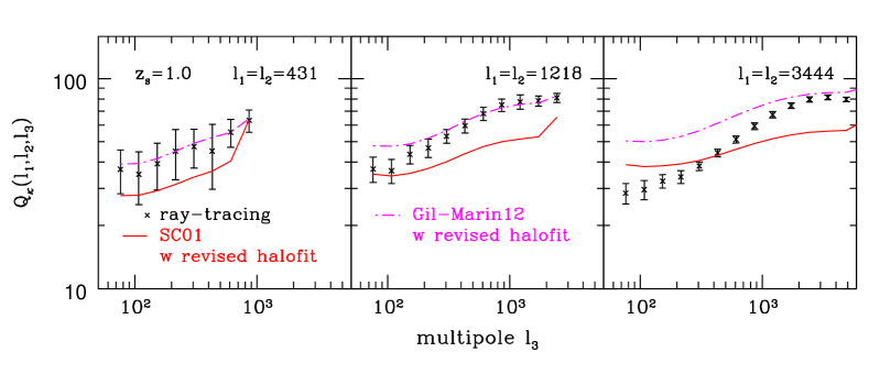
The right panel in Figure 2 shows the reduced convergence bispectrum $Q_{\kappa}$ measured from the ray-tracing simulations averaged over 1000 realizations at source redshift $z_{s}=1.0$ for equilateral triangles. The symbols and lines are the same as in the left panel. First, as expected, this quantity is much less sensitive to the choice of the power spectrum used in the formulas. Our simulation results are consistent with the Gil-Marin12 fitting formula results up to $l\lower 2.15277pt\hbox{$\;\buildrel<\over{\sim}\;$}4000$ within the error bars, whereas SC01 fitting formula underestimates the amplitude of the reduced convergence bispectrum for equilateral triangles, although the broadband shape looks very similar to Gil-Marin12 fitting formula. This is probably because Gil-Marin12 use simulations with more particles in larger boxes, and they performed more realizations compared with SC01, which results in a great improvement in estimation of the bispectrum. Therefore, Gil-Marin12 fitting formula is more suitable to estimate the bispectrum and gives larger power than SC01 fitting formula. Note also that as shown in Figures 1 and 2 in Valageas et al. (2012a), we can also accurately predict the reduced bispectrum using the combined theory.

The power and bispectrum obtained from simulations are underestimated at scales $l>6000$ and $l>4000$ due to the triangular shaped cloud assignment scheme used to obtain two-dimensional gravitational potential of the lens plane (see Sato et al. (2009)).

IV.3 Weak lensing bispectra for isosceles triangles

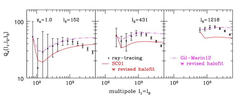
In Figures 3 and 4, we show the reduced convergence bispectrum $Q_{\kappa}$ at source redshift $z_{s}=1.0$ for isosceles triangles, where $l_{1}=l_{2}$. As for the equilateral configurations shown in Figure 2, the tree-level perturbation theory does not show a good agreement, and we thus do not plot it. We also do not plot results of fitting formulas with halofit, because both the results with revised halofit and with halofit are nearly identical. In the Figure 3, where $l_{3}=152$ (left panel), $l_{3}=431$ (middle panel), and $l_{3}=1218$ (right panel), we find that Gil-Marin12 fitting formula well reproduces the simulation results up to $l_{1}=l_{2}\sim 1000$, while SC01 fitting formula agrees with simulation results up to $l_{1}=l_{2}\sim 300$ and underestimates the bispectrum in general.

In the Figure 4, we show the dependence on $l_{3}$ for fixed $l_{1}=l_{2}=431$ (left panel), $l_{1}=l_{2}=1218$ (middle panel), $l_{1}=l_{2}=3444$ (right panel). Again, Gil-Marin12 fitting formula is in fairly good agreement with the simulation results except for $l_{1}=l_{2}=3444$, while SC01 fitting formula underestimates the bispectrum in general as in Figure 3. Gil-Marin12 fitting formula generally deviates from simulation results in squeezed configurations $l_{1}=l_{2}\lower 2.15277pt\hbox{$\;\buildrel>\over{\sim}\;$}10\,l_{3}$. Note that the combined theory provides a better match to the simulation results even in squeezed configurations $l_{1}=l_{2}\lower 2.15277pt\hbox{$\;\buildrel>\over{\sim}\;$}10\,l_{3}$, as shown in Figure 3 in Valageas et al. (2012a).

V Covariance matrix of weak lensing bispectrum

In this section, we investigate how large the non-Gaussian error of the covariance matrix of the lensing bispectrum is, compared to the Gaussian error. We focus on the results of equilateral configurations. See Kayo et al. (2013) for the bispectrum covariance matrix of nonequilateral triangle configurations.

V.1 Diagonal components of the covariance matrix

Figure 5: Diagonal components of the covariance matrix of the lensing bispectrum with and without shape noise at source redshifts $z_{s}=0.6,1.0$ and 1.5 for equilateral triangles. The results are divided by Gaussian covariances denoted by the first term on the right-hand side of Equation (12). Therefore, the deviations from unity arise from the non-Gaussian error of the covariance.

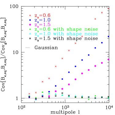
Figure 5 shows the diagonal elements of the covariance matrix for the convergence bispectrum with and without shape noise contamination. We plot the results for equilateral triangles at $z_{s}=0.6$, 1.0, and 1.5 as a function of multipole. The values are divided by the Gaussian contribution of the covariance matrix, which is computed by inserting the nonlinear power spectrum measured from the ray-tracing simulations into the first term in the right-hand side of Equation (12). Thus, the relative amplitude of the non-Gaussian terms is indicated by the deviation from unity in this figure. When we neglect the shape noise effect, we can see that the non-Gaussian terms become significant at multipoles of a few hundreds, and then they dominate over the Gaussian component on smaller scales and at lower source redshifts due to the nonlinear evolution of the matter clustering. This trend is similar to that in the power spectrum covariance examined in Sato et al. (2009) (see Figure 6 in that paper).

However, when we add realistic shape noise contamination described in Section III.1, the values significantly decline and approach to unity irrespective to the source redshift. This result is attributed to the fact that the shape noise dominates the total error budget, which follows Gaussian statistics and contributes to the both numerator and denominator. Although the importance of the non-Gaussian terms are largely degraded in the presence of the shape noise, we will later show that the impact of the non-Gaussian error can remain significant in terms of the signal-to-noise ratio as well as the estimated error on the cosmological parameters.

V.2 Off-diagonal components of the covariance matrix

Figure 6: Correlation coefficient matrices of the bispectrum covariance obtained from large number of ray-tracing simulations with (upper triangular parts of the matrices) and without shape noise (lower triangular parts) at source redshift $z_{s}=0.6,1.0$ and 1.5 for equilateral triangles.

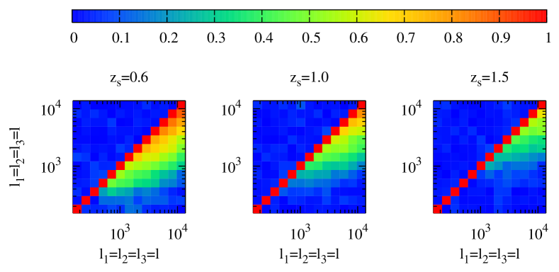
The correlation coefficient between the convergence bispectrum covariances at different triangular shapes quantifies the relative strength of the off-diagonal component to the diagonal component. We define the correlation coefficient as

$$r[B_{\kappa}(l_{1},l_{2},l_{3}),B_{\kappa}(l_{1}^{\prime},l_{2}^{\prime},l_{3}^{\prime})]=\frac{{\rm Cov}[B_{\kappa}(l_{1},l_{2},l_{3}),B_{\kappa}(l_{1}^{\prime},l_{2}^{\prime},l_{3}^{\prime})]}{\sqrt{{\rm Cov}[B_{\kappa}(l_{1},l_{2},l_{3}),B_{\kappa}(l_{1},l_{2},l_{3})]{\rm Cov}[B_{\kappa}(l_{1}^{\prime},l_{2}^{\prime},l_{3}^{\prime}),B_{\kappa}(l_{1}^{\prime},l_{2}^{\prime},l_{3}^{\prime})]}},$$ (23)

where $l_{1}=l_{1}^{\prime}$, $l_{2}=l_{2}^{\prime}$, and $l_{3}=l_{3}^{\prime}$ gives the diagonal components, which equal to unity by definition. For the off-diagonal components $r\sim 1$ ($-1$) means a strong (anti-) correlation between the two triangles, while $r=0$ means two triangles are statistically uncorrelated.

Figure 6 shows the correlation coefficient matrices of the weak lensing bispectrum for equilateral configurations at $z_{s}=0.6$, 1.0, and 1.5. The upper triangular parts of the matrices are the results including the shape noise, while the lower triangular parts ignore that. In the absence of shape noise, the correlation is stronger at higher multipoles and at lower redshifts, as expected. Compared to the results in the power spectrum case (see Figure 8 in Sato et al. (2009)), the relative strength of off-diagonal parts is weaker than that of the power spectrum. Strictly speaking, the result depends on the bin widths but the above statement should be true, because the bin widths are almost the same ($\Delta\ln{l}\approx 0.35$ in this paper while $\Delta\ln{l}=0.3$ in Sato et al. (2009)). Considering a realistic shape noise expected in a future weak lensing survey, we can clearly see that the non-Gaussian corrections quickly diminish and the off-diagonal components approach to zero.

VI Signal-to-noise ratio

Although we have shown the impact of the non-Gaussian correction to the covariance matrix for each element, it is not clear how important it is to understand the whole statistical property of the convergence field. One of useful quantities to see this is that the signal-to-noise ratio ($S/N$) of the spectra that quantifies the significance of the fluctuation. The $S/N$s of tomographic lensing power spectrum and bispectrum are defined as (e.g., Takada and Jain, 2004),

$$\left(\left.\frac{S}{N}\right)^{2}\right|_{P_{\kappa}}=\sum_{l,l^{\prime}\leq l_{\rm max}}\sum_{z_{s},z_{s}^{\prime}}{P}_{\kappa,z_{s}}(l){\rm Cov}^{-1}(l,z_{s},l^{\prime},z_{s}^{\prime}){P}_{\kappa,z_{s}^{\prime}}(l^{\prime}),$$ (24)

and

$$\left(\left.\frac{S}{N}\right)^{2}\right|_{B_{\kappa}}=\sum_{\begin{subarray}{c}l_{1}\leq l_{2}\leq l_{3}\leq l_{\rm max}\\ l_{1}^{\prime}\leq l_{2}^{\prime}\leq l_{3}^{\prime}\leq l_{\rm max}\end{subarray}}\sum_{z_{s},z_{s}^{\prime}}{B}_{\kappa,z_{s}}(l_{1},l_{2},l_{3}){\rm Cov}^{-1}(l_{1},l_{2},l_{3},z_{s},l_{1}^{\prime},l_{2}^{\prime},l_{3}^{\prime},z_{s}^{\prime}){B}_{\kappa,z_{s}^{\prime}}(l_{1}^{\prime},l_{2}^{\prime},l_{3}^{\prime}),$$ (25)

where ${\rm Cov^{-1}}$ is the inverse of the covariance matrix and we take account of the bins of the power and bispectrum in the range $72\lower 2.15277pt\hbox{$\;\buildrel<\over{\sim}\;$}l\leq l_{\rm max}$ ($l=72$ is the fundamental mode of our ray-tracing simulations, $l_{\rm f}\simeq 2\pi/5^{\circ}\simeq 72$). We impose the condition $l_{1}\leq l_{2}\leq l_{3}$ for the bispectrum so that every triangle configuration is counted just once. The $S/N$s are expected to be independent of the bin width, as long as the convergence power and bispectrum do not rapidly vary within bin width, or, in other words, the bins are thin enough.

We can also define a similar quantity for a joint measurement of the lensing power and bispectrum tomography. When we consider the nonlinear growth of the matter density field, it is easy to show that the two spectra are not independent each other and thus the total $S/N$ is not a sum of two $S/N$s due to the existence of the cross covariance between the lensing power spectrum and bispectrum. We define the data vector for the joint measurement as

$$\mathbf{D}=\left\{[P_{\kappa}^{1},P_{\kappa}^{2},\cdots,P_{\kappa}^{n_{P}}]_{z_{s}=0.6},\cdots,[P_{\kappa}^{1},P_{\kappa}^{2},\cdots,P_{\kappa}^{n_{P}}]_{z_{s}=1.5},[B_{\kappa}^{1},B_{\kappa}^{2},\cdots,B_{\kappa}^{n_{B}}]_{z_{s}=0.6},\cdots,[B_{\kappa}^{1},B_{\kappa}^{2},\cdots,B_{\kappa}^{n_{B}}]_{z_{s}=1.5}\right\},$$ (26)

where the indices $n_{P}$ and $n_{B}$ are numbers of bins for the power and bispectra. The covariance matrix of the vector $\mathbf{D}$ can be expressed as

$$\mathbf{Cov^{P_{\kappa}+B_{\kappa}}}=\begin{pmatrix}\mathbf{Cov^{P_{\kappa}}}&\mathbf{Cov^{P_{\kappa}B_{\kappa}}}\\ \mathbf{Cov^{P_{\kappa}B_{\kappa}}}&\mathbf{Cov^{B_{\kappa}}}\end{pmatrix},$$ (27)

where $\mathbf{Cov^{P_{\kappa}B_{\kappa}}}$ is the cross covariance between the lensing power and bispectrum. The $S/N$ for the combined measurement is then defined as

$$\left(\left.\frac{S}{N}\right)^{2}\right|_{P_{\kappa}+B_{\kappa}}=\sum_{l,l^{\prime}\leq l_{\rm max}}\sum_{z_{s},z_{s}^{\prime}}{D}_{l,z_{s}}\left[\mathbf{Cov}^{\mathbf{P_{\kappa}+B_{\kappa}}}_{l,l^{\prime},z_{s},z_{s}^{\prime}}\right]^{-1}{D}_{l^{\prime},z_{s}^{\prime}}.$$ (28)

Figure 7: The cumulative signal-to-noise ratios ($S/N$s) for the convergence power spectrum $P_{\kappa}$, bispectrum $B_{\kappa}$ and their joint measurement $P_{\kappa}+B_{\kappa}$ for tomography with three source redshifts. The spectra information over a range of multipoles $72\leq l\leq l_{\rm max}$ is included. The box, circle and cross symbols are the simulation results for the $S/N$s of the power spectra, the bispectra and the joint measurements of the power spectra and bispectra, respectively. The dashed, dotted and solid curves show the $S/N$s of the power spectra and bispectra and the joint measurement for the Gaussian covariance cases. We assume $\Omega_{\rm s}=1500$ deg² for the HSC survey and include the shot noise contamination to the covariance matrices.

According to Hartlap et al. (2007), the inverse of an unbiased estimator of Cov does not yield an unbiased inverse covariance matrix, Cov^-1, in general, although we have adopted an unbiased estimator of the covariance matrix described in Section III.2. When the number of independent realizations are not so large compared to the dimension of the covariance matrix, the inverse of the resulting covariance matrix, which will be used for $S/N$s and the Fisher matrix analysis, would be overestimated, leading to incorrectly tight constraints on the cosmological parameters. Therefore we would like to correct this effect by multiplying a factor shown in Hartlap et al. (2007). For $N_{R}$ independent simulations, an unbiased estimator of the inverse covariance is as follows (e.g., Hartlap et al., 2007; Taylor et al., 2012):

$${\rm Cov}^{-1}|_{\rm unbiased}=\frac{N_{R}-p-2}{N_{R}-1}{\rm Cov}^{-1}$$ (29)

for $N_{R}-2>p$, where $p$ is the number of bins in the spectra. For our tomographic analysis with $l_{\rm max}=2000$, the dimensions of the resulting covariance matrices are $30\times 30$, $345\times 345$, and $375\times 375$ for the power spectrum, bispectrum, and their joint covariance, respectively. With our 1000 independent realizations ($N_{R}=1,000$), the correction factor can be important especially when we take the bispectrum into account. Therefore, we correct the inverse covariance matrix by using the above equation.

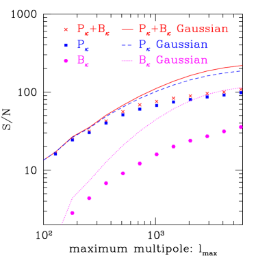
Figure 7 shows the $S/N$s for the measurements of the power spectra, bispectra, and their joint analysis for a tomographic survey with $\Omega_{\rm s}=1500$ deg² area as a function of the maximum multipole $l_{\rm max}$. We simply scale each component of the covariances to obtain the predictions for $\Omega_{\rm s}=1500$ deg², as described in Section III.1. Note that we include the shot noise contamination to the covariance matrices in this figure. The box, circle and cross symbols are the simulation results for the $S/N$s of the power spectra, the bispectra and their joint measurement respectively. The dashed, dotted and solid curves show the respective $S/N$s when only the Gaussian term is included in the covariance matrix. Our simulation results show that the true $S/N$s with a correct non-Gaussian covariance deviate significantly from that with the Gaussian covariance. The impact of the non-Gaussian covariance to the total information content is larger for the bispectrum than for the power spectrum when all the triangle configurations are taken into account. It degrades the $S/N$ by a factor of 3 (2) for the bispectrum (power spectrum) at $l\leq l_{\rm max}=2000$. The bispectrum adds a new information to the power spectrum and increases the value of $S/N$ by about 10% for this $l_{\rm max}$ compared to the power spectrum measurement alone. Note that $l_{\rm max}\sim 2000$ is a typical maximum multipole for the upcoming surveys and above that multipole we cannot gain much information because of the large shot noise contamination as shown in the figure. The trend that the $S/N$s do not increase significantly at multipoles $l\lower 2.15277pt\hbox{$\;\buildrel>\over{\sim}\;$}$ 1000 due to the non-Gaussian contribution and shape noise contamination is similar to the results by Kayo et al. (2013) in which the $S/N$ is examined for a single source plane without tomography.

VII Fisher matrix analysis

Figure 8: Derivatives of the convergence power spectrum (left panel) and bispectrum (right panel) with respect to various cosmological parameters at $z_{s}=1.0$. The symbols are the results from ray-tracing simulations with different cosmological parameters. The solid curves are the results of revised halofit for the power spectrum and Gil-Marin12 with revised halofit for the bispectrum. The dashed curves are the same as the solid curves, but we use the central difference method (Equation 30) with the same step sizes $h_{\alpha}$ used for the simulations.

Figure 9: Cosmological parameter constraints from the lensing power spectrum tomography using the non-Gaussian (red) and Gaussian (blue) covariance matrices. Top panel: without shape noise. Bottom panel: with shape noise. We use the power spectrum information up to $l_{\rm max}=2000$ assuming a survey area of 1500deg².

In this section, we employ the Fisher matrix analysis to show how much cosmological information we can extract from the convergence power and bispectrum with a special attention to the impact of non-Gaussian error contribution. Although the Fisher matrix forecast involves some approximations, Wolz et al. (2012) recently showed that it would be accurate enough for the predictions of the cosmological constraints from weak lensing surveys because the likelihood function is close to multivariate Gaussian. The Markov Chain Monte Carlo method is more robust by direct sampling of the full likelihood function without approximations (e.g., Lewis and Bridle, 2002; Sato et al., 2010, 2011b). In this paper, however, we simply propagate the errors on the convergence power spectrum and/or bispectrum into projections of cosmological parameters using a Fisher information matrix formalism.

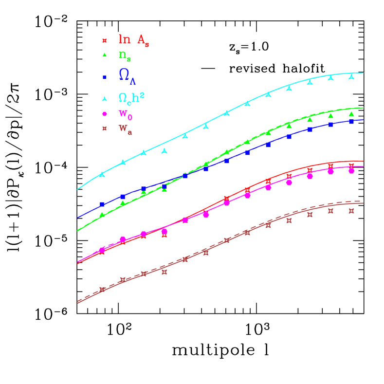
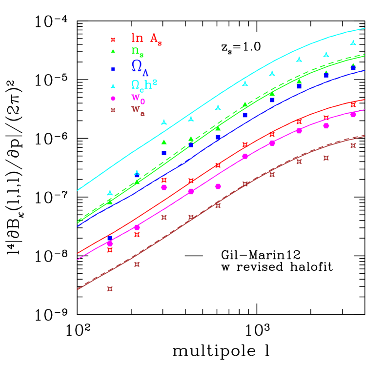
In the Fisher analysis, we need derivatives of the spectra with respect to the cosmological parameters as well as the covariance matrix. We estimate the derivatives by taking the difference of the spectra from ray-tracing simulations with different cosmological parameters. We first discuss this numerical derivatives before showing the results of the Fisher analysis. Figure 8 shows the derivatives of the convergence power spectrum (left panel) and bispectrum (right panel) with respect to six cosmological parameters in absolute values at $z_{s}=1.0$. To calculate the numerical derivatives, we use central difference method defined as

$$\frac{\partial{X}_{\kappa,z_{s}}({\bm{p}})}{\partial p_{\alpha}}=\frac{X_{\kappa,z_{s}}(p_{\alpha}+h_{\alpha})-X_{\kappa,z_{s}}(p_{\alpha}-h_{\alpha})}{2h_{\alpha}},$$ (30)

where $X_{\kappa,z_{s}}$ denotes the convergence power or bispectrum and $h_{\alpha}$ denotes the variations of the cosmological parameters $p_{\alpha}$. In this paper, we choose $h_{\alpha}$ to be 10% of the fiducial values of $p_{\alpha}$, but $h_{\alpha}=0.5$ for $w_{a}$ as described in Section III.1. The solid lines show the predictions of the fitting formulas (revised halofit for left panel and Gil-Marin12 with revised halofit for right panel) obtained using the central difference method to calculate the derivatives with a very small variation $h_{\alpha}$. The dashed lines are the same as the solid lines, but we use same $h_{\alpha}$ values used in the simulations in order to show the convergence of our numerical derivatives. Both solid and dashed lines coincide with each other, although small differences can be seen in $n_{s}$ and $w_{a}$. For both the power and bispectrum, the fitting formulas show good agreement with simulation results, although we can see large scatters around the results of the fitting formula of bispectrum on large scales probably because of the small number of realizations (i.e., $40$ realizations). We will discuss the impact of the step sizes of the central difference method and scatters of the bispectrum on cosmological parameter estimation below around Figure 10.

We now consider a power spectrum analysis based on a tomographic survey with three source redshifts. Using the numerical nonlinear derivatives and the measured covariance matrices, we can calculate the Fisher information matrix as (e.g., Tegmark et al., 1997; Kiessling et al., 2011)

$$F_{\alpha\beta}^{P_{\kappa}}=\sum_{l,l^{\prime}\leq l_{\rm max}}\sum_{z_{s},z_{s}^{\prime}}\frac{\partial{P}_{\kappa,z_{s}}(l)}{\partial p_{\alpha}}{\rm Cov}^{-1}(l,z_{s},l^{\prime},z_{s}^{\prime})\frac{\partial{P}_{\kappa,z_{s}^{\prime}}(l^{\prime})}{\partial p_{\beta}},$$ (31)

where we assume that the cosmology dependence of the covariance matrix can be neglected. We choose $l_{\rm max}=2000$ for our analysis. The error on the $\alpha$th parameter including marginalization over uncertainties in other parameters is estimated as $\sigma(p_{\alpha})=\sqrt{({\boldsymbol{F}^{-1}})_{\alpha\alpha}}$, where ${\boldsymbol{F}^{-1}}$ is the inverse of the Fisher matrix.

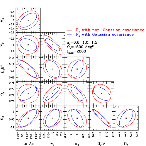
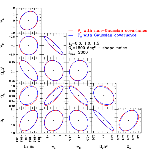
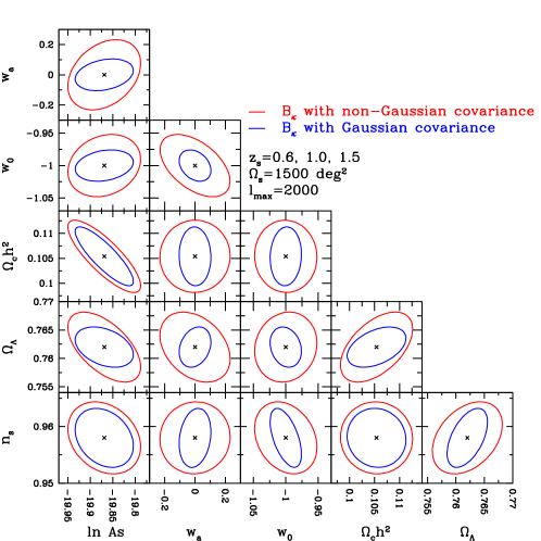
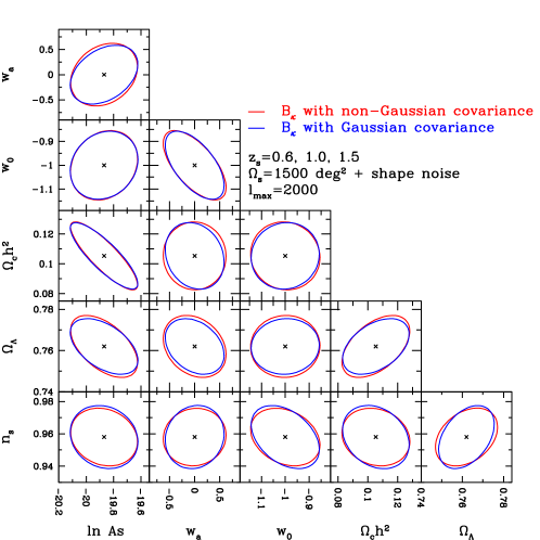
Figure 9 shows the marginalized error constraints with (bottom panel) and without shape noise (top panel) for $\Omega_{\rm s}=1500$deg². The figure shows the marginalized 1$\sigma$ error contours from the weak lensing power spectrum tomography for every pair of six cosmological parameters. The red solid lines show the results obtained when we adopt the non-Gaussian covariance matrix measured from the simulations while the blue solid lines show those with Gaussian covariance matrix. As clearly seen in the top panel of Figure 9, the impact of non-Gaussian errors are crucial for constraining the cosmological parameters accurately in the absence of shape noise. The presence of the non-Gaussian components in the covariance matrix enlarge the error ellipses of the dark energy parameters ($w_{0}$ and $w_{a}$) typically by 40%. However, in the presence of shape noise, the two contours are nearly identical and the impact of the non-Gaussian covariance is small. The largest difference in the parameter constraint is seen in $\Omega_{\Lambda}$, and is about 10%. It might be enough to consider the Gaussian component of the covariance matrix in estimating the cosmological parameters for ongoing surveys, as indicated at the end of Section V depending on at what accuracy one hopes to constrain the parameters. Although current ongoing surveys seem to be fine with the Gaussian approximation in the covariance matrix, it could be crucial to properly take account of the non-Gaussianity for ultimately large survey projects in future.

Figure 10: Same as Figure 9, but result for the weak lensing bispectrum tomography. Top panel: without shape noise. Bottom panel: with shape noise.

As in the convergence power spectrum, the Fisher matrix for the convergence bispectrum tomography is given as

$$F_{\alpha\beta}^{B_{\kappa}}=\sum_{\begin{subarray}{c}l_{1}\leq l_{2}\leq l_{3}\leq l_{\rm max}\\ l_{1}^{\prime}\leq l_{2}^{\prime}\leq l_{3}^{\prime}\leq l_{\rm max}\end{subarray}}\sum_{z_{s},z_{s}^{\prime}}\frac{\partial{B}_{\kappa,z_{s}}(l_{1},l_{2},l_{3})}{\partial p_{\alpha}}{\rm Cov}^{-1}(l_{1},l_{2},l_{3},z_{s},l_{1}^{\prime},l_{2}^{\prime},l_{3}^{\prime},z_{s}^{\prime})\frac{\partial{B}_{\kappa,z_{s}^{\prime}}(l_{1}^{\prime},l_{2}^{\prime},l_{3}^{\prime})}{\partial p_{\beta}},$$ (32)

where we have imposed the condition $l_{1}\leq l_{2}\leq l_{3}$ so that every triangle configuration is counted once.

Figure 10 is the same as Figure 9, but the result for the weak lensing bispectrum tomography. First, we can see that the marginalized error contours for the bispectrum analysis are narrower than those for the power spectrum. This is quite surprising since the bispectrum is higher-order spectrum than the power spectrum, so one might believe that the constraints from the bispectrum are weaker than those from the power spectrum. Indeed, we have shown that the $S/N$ for the bispectrum is smaller than that for the power spectrum in the last section (see Figure 7). The smaller error ellipses from the bispectrum analysis may be attributed to the fact that the bispectrum is more sensitive to the cosmological parameters, since the power spectrum and bispectrum are proportional to $\Omega_{m}^{2}$ and $\Omega_{m}^{3}$, in spite of smaller $S/N$ from the bispectrum. A consistent result, the bispectrum is more powerful to constrain the cosmological parameters, can be found in Bergé et al. (2010), although they did not assume a tomographic survey. We confirmed that this is the case for each of our convergence maps at three source redshifts. Also Kilbinger and Schneider (2005) showed that third-order aperture mass statistics put tighter constraints on cosmological parameters than second-order aperture mass statistics. In contrast, other papers (e.g., Takada and Jain (2004)) presented that the constraint from the lensing bispectrum are comparable to that from the power spectrum. Therefore, other studies need to be done in order to solve this discrepancy.

There are two concerns: the derivatives of the Fisher matrix and the redshift distribution of source galaxies.

• We used only 40 realizations for each of the three source redshifts for varied cosmologies to estimate the derivatives of the Fisher matrix. As shown in Figure 8, the derivatives of the lensing bispectrum estimated in a finite volume have large scatter around theoretical predictions on large scales. The total volume might not be large enough to converge the derivatives with our 40 realizations and this can lead to an inaccurate constraints. Furthermore, we varied each of the cosmological parameters by $\pm$ 10% except for $w_{a}$. From Figure 8, we find that a 10% change in some of the parameters gives a big change in the bispectrum. A $10\%$ change in the spectral index $n_{s}$, especially, results in a $\sim 100\%$ change in the bispectrum from the fiducial cosmology and this might lead to narrower constraints.

• We used three $\delta$-function like source redshift distribution instead of a realistic continuous redshift distribution. To check the impact of this treatment, we analytically calculate the power and bispectrum for two source distributions. We consider source galaxies at exactly $z_{s}=1.0$ and a model redshift distribution of galaxies used in Takada and Jain (2009) (Equation 20 in their paper) where galaxies have a broad distribution in $z_{s}$ with the mean redshift of $z_{s}=1.0$. We found that the amplitudes of the power and bispectrum in the latter case are smaller by $\sim 30\%$ ($\sim 60\%$) for the power (bi-)spectrum and thus the derivatives of the Fisher matrix are smaller correspondingly. Note that the elements of the covariance matrices also become smaller when a realistic source distribution is considered. Therefore, the constraints from the power and bispectrum with a realistic redshift distribution would be weaker than the constraints presented here and this effect should be larger for the bispectrum.

Therefore, we guess that the sizes of the marginalized contours for the bispectrum are misestimated (underestimated, probably) in our analysis. However, our interest here is in how well the approximation of Gaussianity in the covariance matrix is justified for the bispectrum covariance. The above two possible systematics are more related to the derivatives of the bispectrum with respect to the cosmological parameters, and their impact on the non-Gaussian covariance matrix would not be significant.

In the presence of realistic shape noise, the importance of the non-Gaussian errors are degraded, similarly to what we have shown in the power spectrum analysis. Again, one might be able to neglect them for the ongoing surveys, while they might be important for future wide-field surveys.

Figure 11: Cosmological parameter constraints from a combined measurement of the lensing power spectrum and bispectrum tomography using full non-Gaussian covariance (red solid lines) and non-Gaussian covariance without cross-covariance matrix (blue solid lines) in the absence (top panel) and presence of the shape noise contamination (bottom panel), respectively. We use the spectrum information up to $l_{\rm max}=2000$ and assume survey area is 1500deg².

We finally calculate the Fisher matrix for a combined measurement of the lensing power and bispectrum tomography up to $l_{\rm max}=2000$. As in the $S/N$, the total Fisher matrix is not a simple sum of the Fisher matrices of the power and bispectra. By using Equations (26) and (27), the Fisher matrix for the combined measurement is then defined as

$$F_{\alpha\beta}^{P_{\kappa}+B_{\kappa}}=\sum_{i,j\leq l_{\rm max},z_{s}^{\rm max}}\frac{\partial{D}_{i}}{\partial p_{\alpha}}\left[\mathbf{Cov}^{P_{\kappa}+B_{\kappa}}\right]^{-1}_{ij}\frac{\partial{D}_{j}}{\partial p_{\beta}}.$$ (33)

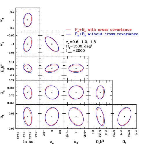
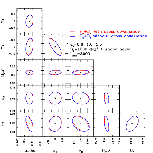
The cosmological parameter constraints from the joint measurement of the lensing power spectrum and bispectrum with (bottom panel) and without (top panel) shape noise for $\Omega_{\rm s}=1500$deg² are shown in Figure 11. The red solid lines are the results calculated using full non-Gaussian covariance matrix including the cross covariance, while the blue solid lines are those using the covariance matrix without the cross covariance between the power and bispectra. As shown by Kayo et al. (2013), the leading contribution to the cross covariance between the two spectra comes from the five-point correlation function, and one might take this as a higher-order effect. The impact of the cross covariance, however, is not so small even in the presence of shape noise, and the difference is more than 20% for $\Omega_{c}h^{2}$ which is well constrained from cosmic microwave background experiments (e.g. WMAP or Planck satellite) though. However, for the dark energy parameters such as $\Omega_{\Lambda}$, $w_{0}$, and $w_{a}$ the difference is only a few percent. Note that the analysis which includes the cross covariance (i.e., the red contours) shows tighter constraints because the cross covariance brings new information. Therefore, when we constrain the dark energy parameters from a combined measurement of the lensing power and bispectra, we can analyze each spectrum independently and then just add information of both spectra to obtain a joint constraint, if one needs a precision of 10% in parameter constraints, because the impact of the cross covariance is only a few percent.

VIII Optimizing the dark energy Figure of Merit

The dark energy figure of merit (FoM) is often used in the literature to characterize the performance of a survey on the dark energy parameter constraints. The dark energy FoM is defined as (Albrecht et al., 2006)

$${\rm FoM}\equiv\frac{1}{\sigma(w_{p})\sigma(w_{a})}=\frac{1}{\sqrt{{\rm det}({\rm Cov}[w_{0},w_{a}])}},$$ (34)

where $w_{p}$ is the equation of state of the dark energy at the pivot redshift, and Cov[$w_{0}$, $w_{a}$] is the $2\times 2$ submatrix of the inverted Fisher matrix, for which we use the same method used in the previous section.

In this section, we examine how FoM scales as a function of the mean number density of source galaxies and the survey area, under the condition that the total observation time is fixed. Following Yamamoto et al. (2007), we express the total survey area $\Omega_{\rm s}$ as

$$\Omega_{\rm s}=\pi\left(\frac{\text{Field of View}}{2}\right)^{2}\frac{T_{\rm total}}{1.1\times\sum_{j}(t_{{\rm exp},j}+t_{{\rm oh},j})},$$ (35)

where we assume HSC wide survey for 200 days in five years with a 1.5 deg field of view and an overhead time $t_{{\rm oh},j}=0.3$ min for each band. We denote by $t_{{\rm exp},j}$ the exposure time for each (the $j$th) band. We compute the total observation time as $T_{\rm total}=200({\rm days})\times 9({\rm hours/days})\times 0.7=1260$ hours, assuming that we take an observation for 9 hours per night, and the fine day rate of $0.7$. We consider the photo-$z$ determination with five bands ($g$, $r$, $i$, $z$, $y$). We fix the exposure time as 10 (20) min for $g$ and $r$ bands ($z$ and $y$ bands), but change the exposure time for $i$ band $t_{{\rm exp},i}$. We relate the mean number density of source galaxies $\bar{n}_{g}$ to the exposure time for $i$ band as (see, HSC white paper).

$$\bar{n}_{g}=30\left(\frac{t_{{\rm exp},i}}{\text{20 minutes}}\right)^{0.44}{\rm arcmin}^{-2}.$$ (36)

We assume for simplicity that the mean source redshift is fixed to $z_{m}$=1.0 regardless of the exposure time.

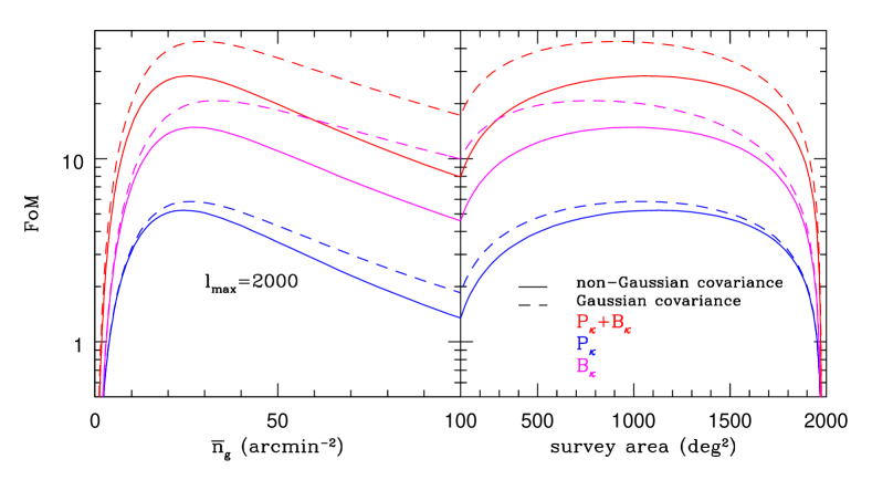
Figure 12 shows the dark energy FoM as a function of the mean number density of source galaxies (left panel) and the survey area (right panel), obtained from the convergence power spectrum $P_{\kappa}$, bispectrum $B_{\kappa}$, and their joint measurement $P_{\kappa}+B_{\kappa}$ for a tomography with three source redshifts under the above condition. We keep the fraction of the number density at the three source redshifts the same as in Section III.1. The solid lines show the results taking account of the non-Gaussian covariance while the dashed lines are obtained for the Gaussian covariance. The optimal survey design can be different from one estimated using a Gaussian covariance, which is often done in the literature, when we appropriately evaluate the non-Gaussian covariance matrix. As shown in the Figure 12, the value of the mean number density (survey area) that gives the maximum FoM is smaller (larger) when the non-Gaussian error is properly taken into account. For the HSC wide survey, the maximum FoM estimated from the joint measurement of the power spectrum and bispectrum tomography is given at $\bar{n}_{g}\sim 25$ arcmin^-2 ($\Omega_{\rm s}\sim 1100$ deg²) whose values are close to the planed values ($\bar{n}_{g}\sim 20$ arcmin^-2, $\Omega_{\rm s}\sim 1400$ deg²) in HSC wide survey  (see, HSC white paper and/or SSP proposal).

Figure 12: The dark energy figure of merit as a function of the mean number density of source galaxies (left panel) and the survey area (right panel), obtained from convergence power spectrum $P_{\kappa}$, bispectrum $B_{\kappa}$, and their joint measurement $P_{\kappa}+B_{\kappa}$ for a tomography with three source redshifts assuming Subaru Hyper Suprime-Cam (HSC) wide survey whose total observation time is fixed. The solid lines are the results of each spectrum considering non-Gaussian covariance while dashed lines are those considering Gaussian covariance.

IX Conclusion and Discussion

We have used the Fisher matrix analysis of a tomographic survey with three source redshifts to study how well the approximation of Gaussianity is valid for constraining the cosmological parameters, by comparing the full covariance matrix obtained from a large number of ray-tracing simulations with a Gaussian covariance. Before examining the non-Gaussian features of the covariance matrix, we compared the lensing power and bispectrum obtained from the ray-tracing simulations with those from several theoretical fitting formulas. The lensing power spectrum measured from our ray-tracing simulations well reproduces the revised halofit by Takahashi et al. (2012) based on high-resolution large-volume $N$-body simulations. For the lensing bispectrum, our ray-tracing simulation result shows a good agreement with the theoretical prediction using a recent fitting formula proposed by Gil-Marín et al. (2012), while the fitting formula proposed by Scoccimarro and Couchman (2001) gives sizable disagreement at multipoles $l\lower 2.15277pt\hbox{$\;\buildrel>\over{\sim}\;$}1000$.

We found that the non-Gaussian covariance can be significant at high multipoles in the absence of the shape noise contamination, while the shape noise expected from a realistic survey adds a large contribution to the Gaussian part (i.e. diagonal components of the covariance), which degrades the relative impact of the non-Gaussian corrections to the covariance. The non-Gaussian components of the bispectrum covariance matrix reduce the cumulative signal-to-noise ratio by a factor of 3 at $l_{\rm max}=2000$ even in the presence of shape noise contamination to the covariance. Thus, they are crucial to estimate the information content of the lensing bispectrum accurately.

Unlike the $S/N$, the non-Gaussian terms in the covariance matrix for the bispectrum degrade the parameter constraints by typically less than 15%, which is much smaller than that in the $S/N$. Following Takada and Jain (2009), these results can be interpreted as follows. If we consider the volume of the Fisher matrix ellipsoid in our six-dimensional parameter space as proportional to the $S/N$ magnitude, the non-Gaussian covariance shrinks the volume by a factor of 3. If all the six principal axes of the Fisher matrix ellipsoid are equally shrunk by the non-Gaussian errors, each parameter error would be degraded by about 15% ($\sim 3^{1/6}-1$), which is close to the degradation shown in Figure 10. When we constrain the dark energy parameters such as $\Omega_{\Lambda}$, $w_{0}$, and $w_{a}$, from a joint measurement of the lensing power and bispectrum, the impact of the cross covariance are only a few percent.

Therefore, the Gaussian approximation of the covariance matrix might be reasonable for constraining the cosmological parameters in the present weak lensing surveys. For future weak lensing surveys, however, the non-Gaussianity would be considerable when we constrain the cosmological parameters with a higher precision.