Indoor Semantic Segmentation
using depth information

Abstract

This work addresses multi-class segmentation of indoor scenes with RGB-D inputs. While this area of research has gained much attention recently, most works still rely on hand-crafted features. In contrast, we apply a multiscale convolutional network to learn features directly from the images and the depth information. We obtain state-of-the-art on the NYU-v2 depth dataset with an accuracy of 64.5%. We illustrate the labeling of indoor scenes in videos sequences that could be processed in real-time using appropriate hardware such as an FPGA.

1 Introduction

The recent release of the Kinect allowed many progress in indoor computer vision. Most approaches have focused on object recognition [1, 14] or point cloud semantic labeling [2], finding their applications in robotics or games [6]. The pioneering work of Silberman et al. [22] was the first to deal with the task of semantic full image labeling using depth information. The NYU depth v1 dataset [22] guathers 2347 triplets of images, depth maps, and ground truth labeled images covering twelve object categories. Most datasets employed for semantic image segmentation [11, 17] present the objects centered into the images, under nice lightening conditions. The NYU depth dataset aims to develop joint segmentation and classification solutions to an environment that we are likely to encounter in the everyday life. This indoor dataset contains scenes of offices, stores, rooms of houses containing many occluded objects unevenly lightened. The first results [22] on this dataset were obtained using the extraction of sift features on the depth maps in addition to the RGB images. The depth is then used in the gradient information to refine the predictions using graph cuts. Alternative CRF-like approaches have also been explored to improve the computation time performances [4]. The results on NYU dataset v1 have been improved by [19] using elaborate kernel descriptors and a post-processing step that employs gPb superpixels MRFs, involving large computation times.

A second version of the NYU depth dataset was released more recently [23], and improves the labels categorization into 894 different object classes. Furthermore, the size of the dataset did also increase, it now contains hundreds of video sequences (407024 frames) acquired with depth maps.

Feature learning, or deep learning approaches are particularly adapted to the addition of new image modalities such as depth information. Its recent success for dealing with various types of data is manifest in speech recognition [13], molecular activity prediction, object recognition [12] and many more applications. In computer vision, the approach of Farabet et al. [8, 9] has been specifically designed for full scene labeling and has proven its efficiency for outdoor scenes. The key idea is to learn hierarchical features by the mean of a multiscale convolutional network. Training networks using multiscales representation appeared also the same year in [3, 21].

When the depth information was not yet available, there have been attempts to use stereo image pairs to improve the feature learning of convolutional networks [16]. Now that depth maps are easy to acquire, deep learning approachs started to be considered for improving object recognition [20]. In this work, we suggest to adapt Farabet et al.’s network to learn more effective features for indoor scene labeling. Our work is, to the best of our knowledge, the first exploitation of depth information in a feature learning approach for full scene labeling.

2 Full scene labeling

2.1 Multi-scale feature extraction

Good internal representations are hierarchical. In vision, pixels are assembled into edglets, edglets into motifs, motifs into parts, parts into objects, and objects into scenes. This suggests that recognition architectures for vision (and for other modalities such as audio and natural language) should have multiple trainable stages stacked on top of each other, one for each level in the feature hierarchy. Convolutional Networks [15] (ConvNets) provide a simple framework to learn such hierarchies of features.

Convolutional Networks are trainable architectures composed of multiple stages. The input and output of each stage are sets of arrays called feature maps. In our case, the input is a color (RGB) image plus a depth (D) image and each feature map is a 2D array containing a color or depth channel of the input RGBD image. At the output, each feature map represents a particular feature extracted at all locations on the input. Each stage is composed of three layers: a filter bank layer, a non-linearity layer, and a feature pooling layer. A typical ConvNet is composed of one, two or three such 3-layer stages, followed by a classification module. Because they are trainable, arbitrary input modalities can be modeled, such as the depth modality that is added to the input channel in this work.

Figure 1: Scene parsing (frame by frame) using a multiscale network and superpixels. The RGB channels of the image and the depth image are transformed through a Laplacian pyramid. Each scale is fed to a 3-stage convolutional network, which produces a set of feature maps. The feature maps of all scales are concatenated, the coarser-scale maps being upsampled to match the size of the finest-scale map. Each feature vector thus represents a large contextual window around each pixel. In parallel, a single segmentation of the image into superpixels is computed to exploit the natural contours of the image. The final labeling is obtained by the aggregation of the classifier predictions into the superpixels.

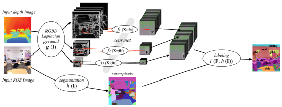
A great gain has been achieved with the introduction of the multiscale convolutional network described in [9]. The multi-scale, dense feature extractor produces a series of feature vectors for regions of multiple sizes centered around every pixel in the image, covering a large context. The multi-scale convolutional net contains multiple copies of a single network that are applied to different scales of a Laplacian pyramid version of the RGBD input image.

The RGBD image is first pre-processed, so that local neighborhoods have zero mean and unit standard deviation. The depth image, given in meters, is treated as an additional channel similarly to any color channel. The overview scheme of our model appears in Figure 1.

Beside the input image which is now including a depth channel, the parameters of the multi-scale network (number of scales, sizes of feature maps, pooling type, etc.) are identical to [9]. The feature maps sizes are 16,64,256, multiplied by the three scales. The size of convolutions kernels are set to 7 by 7 at each layer, and sizes of subsampling kernels (max pooling) are 2 by 2. In our tests we rescaled the images to the size $240\times 320$.

As in [9], the feature extractor followed by a classifier was trained to minimize the negative log-likelihood loss function. The classifier that follows feature extraction is a 2-layer multi-perceptron, with a hidden layer of size 1024. We use superpixels [10] to smooth the convnet predictions as a post-processing step, by agregating the classifiers predictions in each superpixel.

2.2 Movie processing

While the training is performed on single images, we are able to perform scene labeling of video sequences. In order to improve the performances of our frame-by-frame predictions, a temporal smoothing may be applied. In this work, instead of using the frame by frame superpixels as in the previous section, we employ the temporal consistent superpixels of [5]. This approach works in quasi-linear time and reduces the flickering of objects that may appear in the video sequences.

3 Results

We used for our experiments the NYU depth dataset – version 2 – of Silberman and Fergus [23], composed of 407024 couples of RGB images and depth images. Among these images, 1449 frames have been labeled. The object labels cover 894 categories. The dataset is provided with the original raw depth data that contain missing values, with code using [7] to inpaint the depth images.

3.1 Validation on images

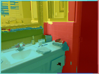
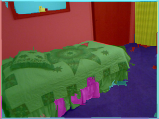
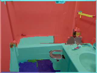
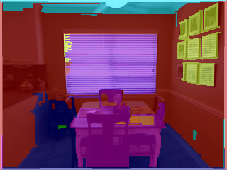
The training has been performed using the 894 categories directly as output classes. The frequencies of object appearences have not been changed in the training process. However, we established 14 clusters of classes categories to evaluate our results more easily. The distributions of number of pixels per class categories are given in Table 1. We used the train/test splits as provided by the NYU depth v2 dataset, that is to say 795 training images and 654 test images. Please note that no jitter (rotation, translations or any other transformation) was added to the dataset to gain extra performances. However, this strategy could be employed in future work. The code consists of Lua scripts using the Torch machine learning software [18] available online at http://www.torch.ch/ .

To evaluate the influence of the addition of depth information, we trained a multiscale convnet only on the RGB channels, and another network using the additional depth information. Both networks were trained until the achievement of their best performances, that is to say for 105 epochs and 98 epochs respectively, taking less than 2 days on a regular server.

We report in Table 1 two different performance measures:

• the “classwise accuracy”, counting the number of correctly classified pixels divided by the number of false positive, averaged for each class. This number corresponds to the mean of the confusion matrix diagonal.

• the “pixelwise accuracy”, counting the number of correctly classified pixels divided by the total number of pixels of the test data.

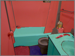
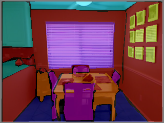
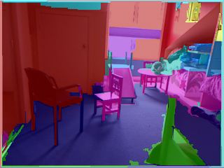
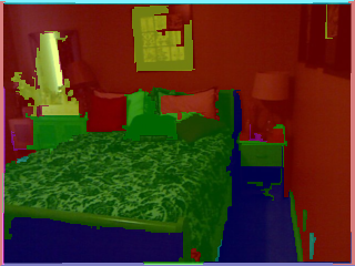
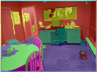
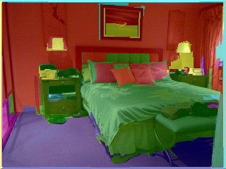
Ground truths

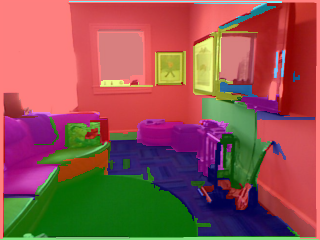
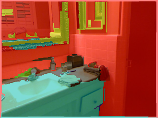
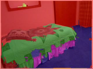
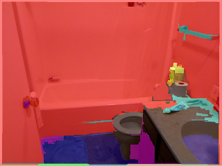
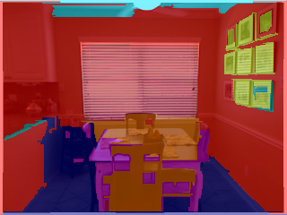
Results using the Multiscale Convnet

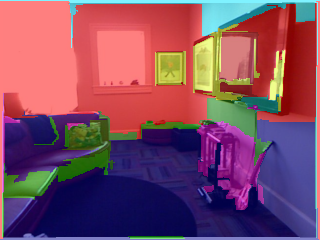
Results using the Multiscale Convnet with depth information

wall bed

books ceiling

chair floor

furniture pict./deco

sofa table

object window

TV uknw

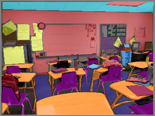
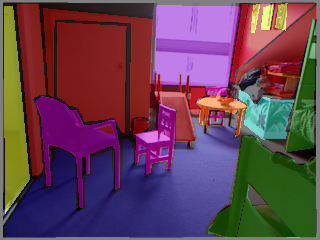
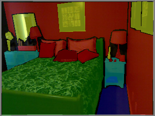
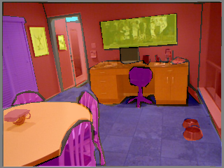
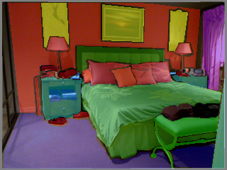
Ground truths

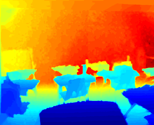
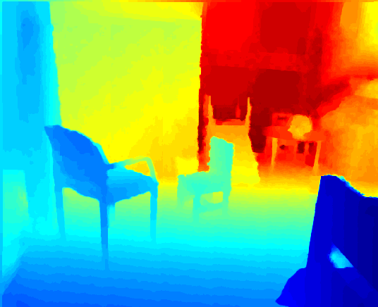
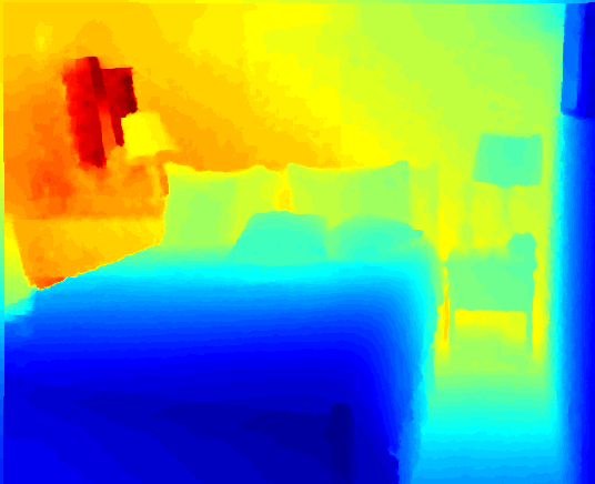
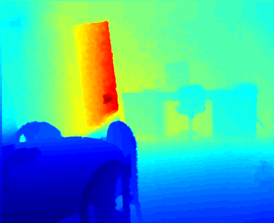
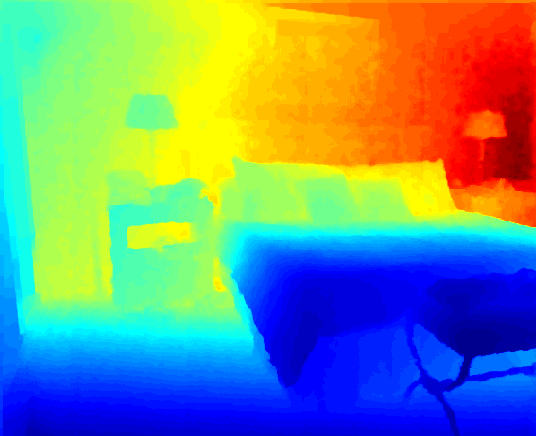
Depth maps

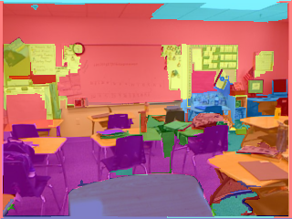
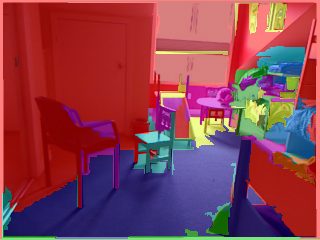
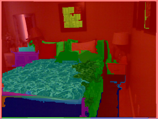
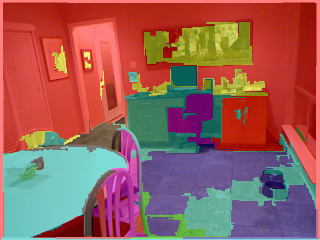
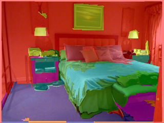
Results using the Multiscale Convnet

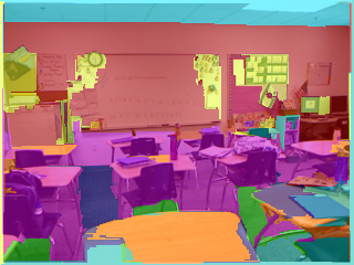
Results using the Multiscale Convnet with depth information

Figure 2: Some scene labelings using our Multiscale Convolutional Network trained on RGB and RGBD images. We observe in Table 1 that adding depth information helps to recognize objects that have low intra-class variance of depth appearance.

We observe that considerable gains (15% or more) are achieved for the classes ’floor’, ’ceiling’, and ’furniture’. This result makes a lot of sense since these classes are characterized by a somehow constant appearance of their depth map. Objects such as TV, table, books can either be located in the foreground as well as in the background of images. On the contrary, the floor and ceiling will almost always lead to a depth gradient always oriented in the same direction: Since the dataset has been collected by a person holding a kinect device at a his chest, floors and ceiling are located at a distance that does not vary to much through the dataset. Figure 2 provides examples of depth maps that illustrate these observations. Overall, improvements induced by the depth information exploitation are present. In the next section, these improvements are more apparent.

	Class	Multiscale	MultiScl. Cnet
	Occurrences	Convnet Acc. [9]	+depth Acc.
bed	4.4%	30.3	38.1
objects	7.1 %	10.9	8.7
chair	3.4%	44.4	34.1
furnit.	12.3%	28.5	42.4
ceiling	1.4%	33.2	62.6
floor	9.9%	68.0	87.3
deco.	3.4%	38.5	40.4
sofa	3.2%	25.8	24.6
table	3.7%	18.0	10.2
wall	24.5%	89.4	86.1
window	5.1%	37.8	15.9
books	2.9%	31.7	13.7
TV	1.0%	18.8	6.0
unkn.	17.8%	-	-
Avg. Class Acc.	-	35.8	36.2
Pixel Accuracy (mean)	-	51.0	52.4
Pixel Accuracy (median)	-	51.7	52.9
Pixel Accuracy (std. dev.)	-	15.2	15.2

Table 1: Class occurrences in the test set – Performances per class and per pixel.

3.2 Comparison with Silberman et al.

In order to compare our results to the state-of-the-art on the NYU depth v2 dataset, we adopted a different selection of outputs instead of the 14 classes employed in the previous section. The work of Silberman et al. [23] defines the four semantic classes Ground, Furniture, Props and Structure. This class selection is adopted in [23] to use semantic labelings of scenes to infer support relations between objects. We recall that the recognition of the semantic categories is performed in [23] by the definition of diverse features including SIFT features, histograms of surface normals, 2D and 3D bounding box dimensions, color histograms, and relative depth.

	Ground	Furniture	Props	Structure	Class Acc.	Pixel Acc.
Silberman et al.[23]	68	70	42	59	59.6	58.6
Multiscale convnet [9]	68.1	51.1	29.9	87.8	59.2	63.0
Multiscale+depth convnet	87.3	45.3	35.5	86.1	63.5	64.5

Table 2: Accuracy of the multiscale convnet compared with the state-of-the-art approach of [23].

As reported in Table 2, the results achieved using the Multiscale convnet are improving the structure class predictions, resulting in a 4% gain in pixelwise accuracy over Silberman et al. approach. Adding the depth information results in a considerable improvement of the ground prediction, and performs also better over the other classes, achieving a 4% gain in classwise accuracy over previous works and improves by almost 6% the pixelwise accuracy compared to Silberman et al.’s results.

We note that the class ’furniture’ in the 4-classes evaluation is different than the ’furniture’ class of the 14-classes evaluation. The furniture-4 class encompasses chairs and beds but not desks, and cabinets for example, explaining a drop of performances here using the depth information.

3.3 Test on videos

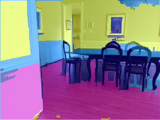
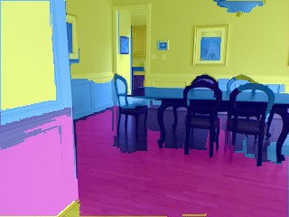
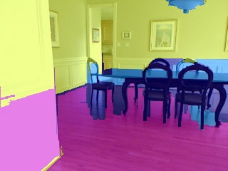
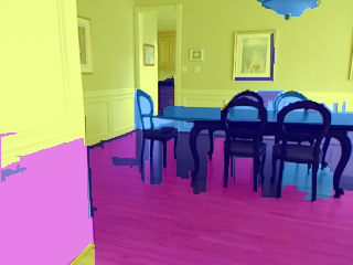
The NYU v2 depth dataset contains several hundreds of video sequences encompassing 26 different classes of indoor scenes, going from bedrooms to basements, and dining rooms to book stores. Unfortunately, no ground truth is yet available to evaluate our performances on this video. Therefore, we only present here some illustrations of the capacity of our model to label these scenes.

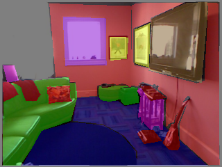
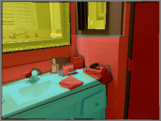
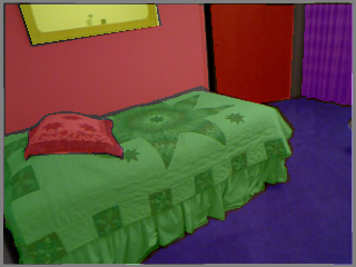
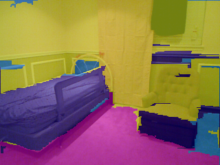
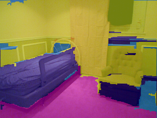
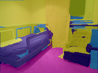
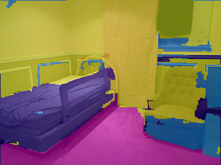
The predictions are computed frame by frame on the videos and are refined using temporally smoothed superpixels using [5]. Two examples of results on sequences are shown at Figure 3.

A great advantage of our approach is its nearly real time capabilities. Processing a 320x240 frame takes 0.7 seconds on a laptop [9]. The temporal smoothing only requires an additional 0.1s per frame.

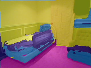
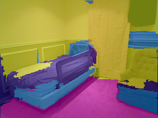
(a) Output of the Multiscale convnet trained using depth information - frame by frame

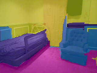
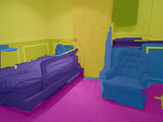
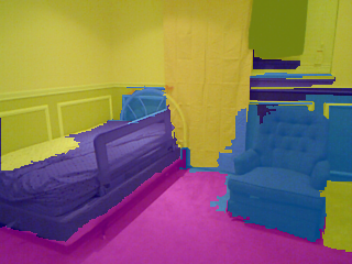
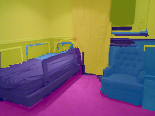
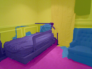
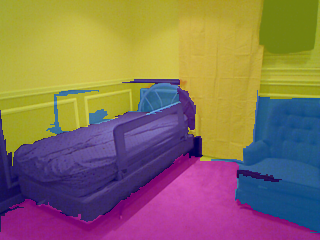
(b) Results smoothed temporally using [5]

Props

Floor

Structure

Wall

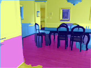
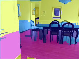
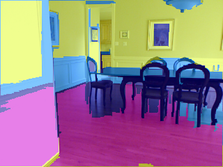
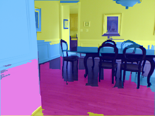
(c) Output of the Multiscale convnet trained using depth information - frame by frame

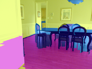
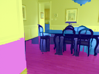
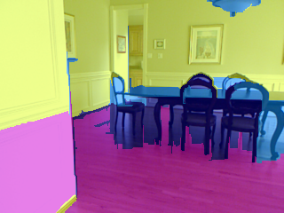
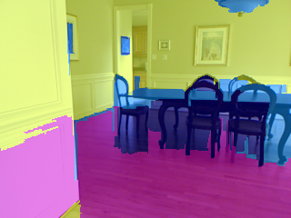
(d) Results smoothed temporally using [5]

Figure 3: Some results on video sequences of the NYU v2 depth dataset. Note that results (c,d) could be improved by using more training examples. Indeed, only a very small number in the labeled training examples exhibit a wall in the foreground.

4 Conclusion

Feature learning is a particularly satisfying strategy to adopt when approaching a dataset that contains new image (or other kind of data) modalities. Our model, while being faster and more efficient than previous approaches, is easier to implement without the need to design specific features adapted to depth information. Different clusterings of object classes as the ones used in this work may be chosen, reflecting this work’s flexibility of applications. For example, using the 4-classes clustering, the accurate results achieved with the multi-scale convolutional network could be applied to perform inference on support relations between objects. Improvements for specific object recognition could further be achieved by filtering the frequency of the training objects. We observe that the recognition of object classes having similar depth appearance and location is improved when using the depth information. On the contrary, it is better to use only RGB information to recognize objects with classes containing high variability of their depth maps. This observation could be used to combine the best results in function of the application. Finally, a number of techniques (unsupervised feature learning, MRF smoothing of the convnet predictions, extension of the training set) would probably help to improve the present system.

5 Acknowledgments

We would like to thank Nathan Silberman for his useful input for handling the NYU depth v2 dataset, and fruitful discussions.

References

- [1] B3do: Berkeley 3-d object dataset. http://kinectdata.com/.
- [2] Cornell-rgbd-dataset. http://pr.cs.cornell.edu/sceneunderstanding/data/data.php.
- [3] Dan Claudiu Ciresan, Alessandro Giusti, Luca Maria Gambardella, and Jürgen Schmidhuber. Deep neural networks segment neuronal membranes in electron microscopy images. In NIPS, pages 2852–2860, 2012.
- [4] Camille Couprie. Multi-label energy minimization for object class segmentation. In 20th European Signal Processing Conference 2012 (EUSIPCO 2012), Bucharest, Romania, August 2012.
- [5] Camille Couprie, Clément Farabet, and Yann LeCun. Causal graph-based video segmentation, 2013. arXiv:1301.1671.
- [6] L. Cruz, D. Lucio, and L. Velho. Kinect and rgbd images: Challenges and applications. SIBGRAPI Tutorial, 2012.
- [7] Anat Levin Dani, Dani Lischinski, and Yair Weiss. Colorization using optimization. ACM Transactions on Graphics, 23:689–694, 2004.
- [8] Clement Farabet, Camille Couprie, Laurent Najman, and Yann LeCun. Scene Parsing with Multiscale Feature Learning, Purity Trees, and Optimal Covers. In Proc. of the 2012 International Conference on Machine Learning, Edinburgh, Scotland, June 2012.
- [9] Clement Farabet, Camille Couprie, Laurent Najman, and Yann LeCun. Learning hierarchical features for scene labeling. IEEE Transactions on Pattern Analysis and Machine Intelligence, 2013. In press.
- [10] Pedro F. Felzenszwalb and Daniel P. Huttenlocher. Efficient graph-based image segmentation. International Journal of Computer Vision, 59:2004, 2004.
- [11] Stephen Gould, Richard Fulton, and Daphne Koller. Decomposing a Scene into Geometric and Semantically Consistent Regions. In IEEE International Conference on Computer Vision, 2009.
- [12] Geoffrey E. Hinton, Nitish Srivastava, Alex Krizhevsky, Ilya Sutskever, and Ruslan Salakhutdinov. Improving neural networks by preventing co-adaptation of feature detectors. CoRR, abs/1207.0580, 2012.
- [13] Navdeep Jaitly, Patrick Nguyen, Andrew Senior, and Vincent Vanhoucke. Application of pretrained deep neural networks to large vocabulary speech recognition. In Proceedings of Interspeech 2012, 2012.
- [14] Allison Janoch, Sergey Karayev, Yangqing Jia, Jonathan T. Barron, Mario Fritz, Kate Saenko, and Trevor Darrell. A category-level 3-d object dataset: Putting the kinect to work. In ICCV Workshops, pages 1168–1174. IEEE, 2011.
- [15] Y. LeCun, L. Bottou, Y. Bengio, and P. Haffner. Gradient-based learning applied to document recognition. Proceedings of the IEEE, 86(11):2278 –2324, nov 1998.
- [16] Yann LeCun, Fu-Jie Huang, and Leon Bottou. Learning Methods for generic object recognition with invariance to pose and lighting. In Proceedings of CVPR’04. IEEE, 2004.
- [17] Ce Liu, Jenny Yuen, and Antonio Torralba. SIFT Flow: Dense Correspondence across Scenes and its Applications. IEEE transactions on pattern analysis and machine intelligence, pages 1–17, August 2010.
- [18] C. Farabet R. Collobert, K. Kavukcuoglu. Torch7: A matlab-like environment for machines learning. In Big Learning Workshop (@ NIPS’11), Sierra Nevada, Spain, 2011.
- [19] Xiaofeng Ren, Liefeng Bo, and D. Fox. Rgb-(d) scene labeling: Features and algorithms. In Computer Vision and Pattern Recognition (CVPR), 2012 IEEE Conference on, pages 2759 –2766, june 2012.
- [20] Richard Socher and Brody Huval and Bharath Bhat and Christopher D. Manning and Andrew Y. Ng. Convolutional-Recursive Deep Learning for 3D Object Classification. In Advances in Neural Information Processing Systems 25. 2012.
- [21] Hannes Schulz and Sven Behnke. Learning object-class segmentation with convolutional neural networks. In 11th European Symposium on Artificial Neural Networks (ESANN), 2012.
- [22] Nathan Silberman and Rob Fergus. Indoor scene segmentation using a structured light sensor. In 3DRR Workshop, ICCV’11, 2011.
- [23] Nathan Silberman, Derek Hoiem, Pushmeet Kohli, and Rob Fergus. Indoor segmentation and support inference from rgbd images. In ECCV, 2012.