Stochastic Pooling for Regularization of
Deep Convolutional Neural Networks
Abstract
We introduce a simple and effective method for regularizing large convolutional neural networks. We replace the conventional deterministic pooling operations with a stochastic procedure, randomly picking the activation within each pooling region according to a multinomial distribution, given by the activities within the pooling region. The approach is hyper-parameter free and can be combined with other regularization approaches, such as dropout and data augmentation. We achieve state-of-the-art performance on four image datasets, relative to other approaches that do not utilize data augmentation.
1 Introduction
Neural network models are prone to over-fitting due to their high capacity. A range of regularization techniques are used to prevent this, such as weight decay, weight tying and the augmentation of the training set with transformed copies [9]. These allow the training of larger capacity models than would otherwise be possible, which yield superior test performance compared to smaller un-regularized models.
Dropout, recently proposed by Hinton et al. [2], is another regularization approach that stochastically sets half the activations within a layer to zero for each training sample during training. It has been shown to deliver significant gains in performance across a wide range of problems, although the reasons for its efficacy are not yet fully understood.
A drawback to dropout is that it does not seem to have the same benefits for convolutional layers, which are common in many networks designed for vision tasks. In this paper, we propose a novel type of regularization for convolutional layers that enables the training of larger models without over-fitting, and produces superior performance on recognition tasks.
The key idea is to make the pooling that occurs in each convolutional layer a stochastic process. Conventional forms of pooling such as average and max are deterministic, the latter selecting the largest activation in each pooling region. In our stochastic pooling, the selected activation is drawn from a multinomial distribution formed by the activations within the pooling region.
An alternate view of stochastic pooling is that it is equivalent to standard max pooling but with many copies of an input image, each having small local deformations. This is similar to explicit elastic deformations of the input images [13], which delivers excellent MNIST performance. Other types of data augmentation, such as flipping and cropping differ in that they are global image transformations. Furthermore, using stochastic pooling in a multi-layer model gives an exponential number of deformations since the selections in higher layers are independent of those below.
2 Review of Convolutional Networks
Our stochastic pooling scheme is designed for use in a standard convolutional neural network architecture. We first review this model, along with conventional pooling schemes, before introducing our novel stochastic pooling approach.
A classical convolutional network is composed of alternating layers of convolution and pooling (i.e. subsampling). The aim of the first convolutional layer is to extract patterns found within local regions of the input images that are common throughout the dataset. This is done by convolving a template or filter over the input image pixels, computing the inner product of the template at every location in the image and outputting this as a feature map , for each filter in the layer. This output is a measure of how well the template matches each portion of the image. A non-linear function is then applied element-wise to each feature map : . The resulting activations are then passed to the pooling layer. This aggregates the information within a set of small local regions, , producing a pooled feature map (of smaller size) as output. Denoting the aggregation function as , for each feature map we have:
| (1) |
where is pooling region in feature map and is the index of each element within it.
The motivation behind pooling is that the activations in the pooled map are less sensitive to the precise locations of structures within the image than the original feature map . In a multi-layer model, the convolutional layers, which take the pooled maps as input, can thus extract features that are increasingly invariant to local transformations of the input image. This is important for classification tasks, since these transformations obfuscate the object identity.
A range of functions can be used for , with and logistic functions being popular choices. In this is paper we use a linear rectification function as the non-linearity. In general, this has been shown [10] to have significant benefits over or logistic functions. However, it is especially suited to our pooling mechanism since: (i) our formulation involves the non-negativity of elements in the pooling regions and (ii) the clipping of negative responses introduces zeros into the pooling regions, ensuring that the stochastic sampling is selecting from a few specific locations (those with strong responses), rather than all possible locations in the region.
There are two conventional choices for : average and max. The former takes the arithmetic mean of the elements in each pooling region:
| (2) |
while the max operation selects the largest element:
| (3) |
Both types of pooling have drawbacks when training deep convolutional networks. In average pooling, all elements in a pooling region are considered, even if many have low magnitude. When combined with linear rectification non-linearities, this has the effect of down-weighting strong activations since many zero elements are included in the average. Even worse, with non-linearities, strong positive and negative activations can cancel each other out, leading to small pooled responses.
While max pooling does not suffer from these drawbacks, we find it easily overfits the training set in practice, making it hard to generalize well to test examples. Our proposed pooling scheme has the advantages of max pooling but its stochastic nature helps prevent over-fitting.
3 Stochastic Pooling
In stochastic pooling, we select the pooled map response by sampling from a multinomial distribution formed from the activations of each pooling region. More precisely, we first compute the probabilities for each region by normalizing the activations within the region:
| (4) |
We then sample from the multinomial distribution based on to pick a location within the region. The pooled activation is then simply :
| (5) |
The procedure is illustrated in Fig. 1. The samples for each pooling region in each layer for each training example are drawn independently to one another. When back-propagating through the network this same selected location is used to direct the gradient back through the pooling region, analogous to back-propagation with max pooling.
Max pooling only captures the strongest activation of the filter template with the input for each region. However, there may be additional activations in the same pooling region that should be taken into account when passing information up the network and stochastic pooling ensures that these non-maximal activations will also be utilized.

3.1 Probabilistic Weighting at Test Time
Using stochastic pooling at test time introduces noise into the network’s predictions which we found to degrade performance (see Section 4.7). Instead, we use a probabilistic form of averaging. In this, the activations in each region are weighted by the probability (see Eqn. 4) and summed:
| (6) |
This differs from standard average pooling because each element has a potentially different weighting and the denominator is the sum of activations , rather than the pooling region size . In practice, using conventional average (or sum) pooling results in a huge performance drop (see Section 4.7).
Our probabilistic weighting can be viewed as a form of model averaging in which each setting of the locations in the pooling regions defines a new model. At training time, sampling to get new locations produces a new model since the connection structure throughout the network is modified. At test time, using the probabilities instead of sampling, we effectively get an estimate of averaging over all of these possible models without having to instantiate them. Given a network architecture with different pooling regions, each of size , the number of possible models is where can be in the - range and is typically 4,9, or 16 for example (corresponding to , or pooling regions). This is a significantly larger number than the model averaging that occurs in dropout [2], where always (since an activation is either present or not). In Section 4.7 we confirm that using this probability weighting achieves similar performance compared to using a large number of model instantiations, while requiring only one pass through the network.
Using the probabilities for sampling at training time and for weighting the activations at test time leads to state-of-the-art performance on many common benchmarks, as we now demonstrate.
4 Experiments
4.1 Overview
We compare our method to average and max pooling on a variety of image classification tasks. In all experiments we use mini-batch gradient descent with momentum to optimize the cross entropy between our network’s prediction of the class and the ground truth labels. For a given parameter at time the weight updates added to the parameters, are where is the gradient of the cost function with respect to that parameter at time averaged over the batch and is a learning rate set by hand.
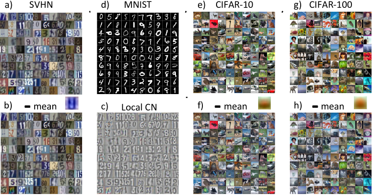
All experiments were conducted using an extremely efficient C++ GPU convolution library [6] wrapped in MATLAB using GPUmat [14], which allowed for rapid development and experimentation. We begin with the same network layout as in Hinton et al. ’s dropout work [2], which has convolutional layers with 5x5 filters and feature maps per layer with rectified linear units as their outputs. We use this same model and train for 280 epochs in all experiments aside from one additional model in Section 4.5 that has 128 feature maps in layer 3 and is trained for 500 epochs. Unless otherwise specified we use pooling with stride (i.e. neighboring pooling regions overlap by element along the borders) for each of the pooling layers. Additionally, after each pooling layer there is a response normalization layer (as in [2]), which normalizes the pooling outputs at each location over a subset of neighboring feature maps. This typically helps training by suppressing extremely large outputs allowed by the rectified linear units as well as helps neighboring features communicate. Finally, we use a single fully-connected layer with soft-max outputs to produce the network’s class predictions. We applied this model to four different datasets: MNIST, CIFAR-10, CIFAR-100 and Street View House Numbers (SVHN), see Fig. 2 for examples images.
4.2 CIFAR-10
We begin our experiments with the CIFAR-10 dataset where convolutional networks and methods such as dropout are known to work well [2, 5]. This dataset is composed of 10 classes of natural images with 50,000 training examples in total, 5,000 per class. Each image is an RGB image of size 32x32 taken from the tiny images dataset and labeled by hand. For this dataset we scale to [0,1] and follow Hinton et al. ’s [2] approach of subtracting the per-pixel mean computed over the dataset from each image as shown in Fig. 2(f).
Cross-validating with a set of 5,000 CIFAR-10 training images, we found a good value for the learning rate to be for convolutional layers and for the final softmax output layer. These rates were annealed linearly throughout training to of their original values. Additionally, we found a small weight decay of to be optimal and was applied to all layers. These hyper-parameter settings found through cross-validation were used for all other datasets in our experiments.
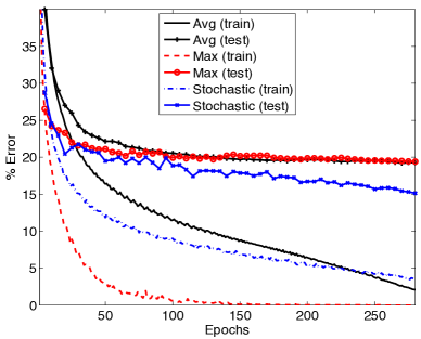
Using the same network architecture described above, we trained three models using average, max and stochastic pooling respectively and compare their performance. Fig. 1 shows the progression of train and test errors over 280 training epochs. Stochastic pooling avoids over-fitting, unlike average and max pooling, and produces less test errors. Table 1 compares the test performance of the three pooling approaches to the current state-of-the-art result on CIFAR-10 which uses no data augmentation but adds dropout on an additional locally connected layer [2]. Stochastic pooling surpasses this result by 0.47% using the same architecture but without requiring the locally connected layer.
| Train Error % | Test Error % | |
| 3-layer Conv. Net [2] | – | |
| 3-layer Conv. Net + 1 Locally Conn. layer with dropout [2] | – | |
| Avg Pooling | ||
| Max Pooling | ||
| Stochastic Pooling | 15.13 |
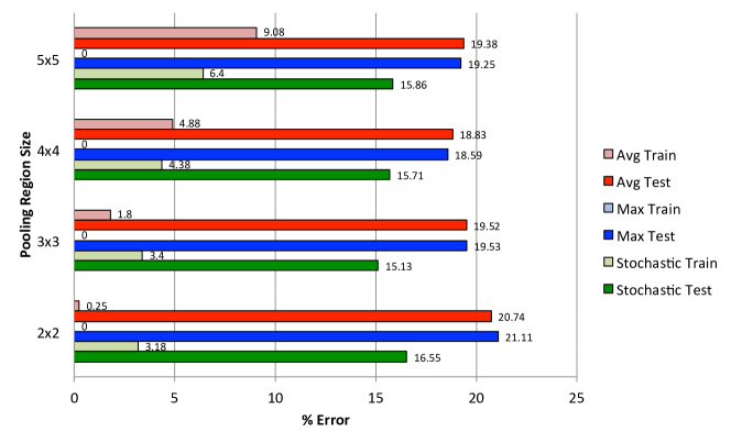
To determine the effect of the pooling region size on the behavior of the system with stochastic pooling, we compare the CIFAR-10 train and test set performance for 5x5, 4x4, 3x3, and 2x2 pooling sizes throughout the network in Fig. 4. The optimal size appears to be 3x3, with smaller regions over-fitting and larger regions possibly being too noisy during training. At all sizes the stochastic pooling outperforms both max and average pooling.
4.3 MNIST
The MNIST digit classification task is composed of 28x28 images of the 10 handwritten digits [8]. There are 60,000 training images with 10,000 test images in this benchmark. The images are scaled to [0,1] and we do not perform any other pre-processing.
During training, the error using both stochastic pooling and max pooling dropped quickly, but the latter completely overfit the training data. Weight decay prevented average pooling from over-fitting, but had an inferior performance to the other two methods. Table 2 compares the three pooling approaches to state-of-the-art methods on MNIST, which also utilize convolutional networks. Stochastic pooling outperforms all other methods that do not use data augmentation methods such as jittering or elastic distortions [7]. The current state-of-the-art single model approach by Cireşan et al. [1] uses elastic distortions to augment the original training set. As stochastic pooling is a different type of regularization, it could be combined with data augmentation to further improve performance.
| Train Error % | Test Error % | |
| 2-layer Conv. Net + 2-layer Classifier [3] | – | |
| 6-layer Conv. Net + 2-layer Classifier + elastic distortions [1] | – | |
| Avg Pooling | ||
| Max Pooling | ||
| Stochastic Pooling | 0.47 |
4.4 CIFAR-100
The CIFAR-100 dataset is another subset of the tiny images dataset, but with 100 classes [5]. There are 50,000 training examples in total (500 per class) and 10,000 test examples. As with the CIFAR-10, we scale to [0,1] and subtract the per-pixel mean from each image as shown in Fig. 2(h). Due to the limited number of training examples per class, typical pooling methods used in convolutional networks do not perform well, as shown in Table 3. Stochastic pooling outperforms these methods by preventing over-fitting and surpasses what we believe to be the state-of-the-art method by %.
| Train Error % | Test Error % | |
|---|---|---|
| Receptive Field Learning [4] | – | |
| Avg Pooling | ||
| Max Pooling | ||
| Stochastic Pooling | 42.51 |
4.5 Street View House Numbers
The Street View House Numbers (SVHN) dataset is composed of 604,388 images (using both the difficult training set and simpler extra set) and 26,032 test images [11]. The goal of this task is to classify the digit in the center of each cropped 32x32 color image. This is a difficult real world problem since multiple digits may be visible within each image. The practical application of this is to classify house numbers throughout Google’s street view database of images.
We found that subtracting the per-pixel mean from each image did not really modify the statistics of the images (see Fig. 2(b)) and left large variations of brightness and color that could make classification more difficult. Instead, we utilized local contrast normalization (as in [12]) on each of the three RGB channels to pre-process the images Fig. 2(c). This normalized the brightness and color variations and helped training proceed quickly on this relatively large dataset.
Despite having significant amounts of training data, a large convolutional network can still overfit. For this dataset, we train an additional model for 500 epochs with 64, 64 and 128 feature maps in layers 1, 2 and 3 respectively. Our stochastic pooling helps to prevent overfitting even in this large model (denoted 64-64-128 in Table 4), despite training for a long time. The existing state-of-the-art on this dataset is the multi-stage convolutional network of Sermanet et al. [12], but stochastic pooling beats this by % (relative gain of ).
| Train Error % | Test Error % | |
| Multi-Stage Conv. Net + 2-layer Classifier [12] | – | |
| Multi-Stage Conv. Net + 2-layer Classifer + padding [12] | – | |
| 64-64-64 Avg Pooling | ||
| 64-64-64 Max Pooling | ||
| 64-64-64 Stochastic Pooling | ||
| 64-64-128 Avg Pooling | ||
| 64-64-128 Max Pooling | ||
| 64-64-128 Stochastic Pooling | 2.80 |
4.6 Reduced Training Set Size
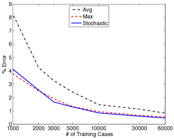
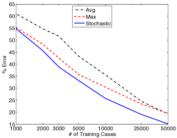
To further illustrate the ability of stochastic pooling to prevent over-fitting, we reduced the training set size on MINST and CIFAR-10 datasets. Fig. 5 shows test performance when training on a random selection of only 1000, 2000, 3000, 5000, 10000, half, or the full training set. In most cases, stochastic pooling overfits less than the other pooling approaches.
4.7 Importance of Model Averaging
To analyze the importance of stochastic sampling at training time and probability weighting at test time, we use different methods of pooling when training and testing on CIFAR-10 (see Table 5). Choosing the locations stochastically at test time degrades performance slightly as could be expected, however it still outperforms models where max or average pooling are used at test time. To confirm that probability weighting is a valid approximation to averaging many models, we draw samples of the pooling locations throughout the network and average the output probabilities from those models (denoted Stochastic- in Table 5). As increases, the results approach the probability weighting method, but have the obvious downside of an -fold increase in computations.
Using a model trained with max or average pooling and using stochastic pooling at test time performs poorly. This suggests that training with stochastic pooling, which incorporates non-maximal elements and sampling noise, makes the model more robust at test time. Furthermore, if these non-maximal elements are not utilized correctly or the scale produced by the pooling function is not correct, such as if average pooling is used at test time, a drastic performance hit is seen.
When using probability weighting during training, the network easily over-fits and performs sub-optimally at test time using any of the pooling methods. However, the benefits of probability weighting at test time are seen when the model has specifically been trained to utilize it through either probability weighting or stochastic pooling at training time.
| Train Method | Test Method | Train Error % | Test Error % |
|---|---|---|---|
| Stochastic Pooling | Probability Weighting | 15.20 | |
| Stochastic Pooling | Stochastic Pooling | ||
| Stochastic Pooling | Stochastic-10 Pooling | ||
| Stochastic Pooling | Stochastic-100 Pooling | 15.12 | |
| Stochastic Pooling | Max Pooling | ||
| Stochastic Pooling | Avg Pooling | ||
| Probability Weighting | Probability Weighting | ||
| Probability Weighting | Stochastic Pooling | ||
| Probability Weighting | Max Pooling | ||
| Probability Weighting | Avg Pooling | ||
| Max Pooling | Max Pooling | ||
| Max Pooling | Stochastic Pooling | ||
| Max Pooling | Probability Weighting | ||
| Avg Pooling | Avg Pooling | ||
| Avg Pooling | Stochastic Pooling | ||
| Avg Pooling | Probability Weighting |
4.8 Visualizations
Some insight into the mechanism of stochastic pooling can be gained by using a deconvolutional network of Zeiler et al. [15] to provide a novel visualization of our trained convolutional network. The deconvolutional network has the same components (pooling, filtering) as a convolutional network but are inverted to act as a top-down decoder that maps the top-layer feature maps back to the input pixels. The unpooling operation uses the stochastically chosen locations selected during the forward pass. The deconvolution network filters (now applied to the feature maps, rather than the input) are the transpose of the feed-forward filters, as in an auto-encoder with tied encoder/decoder weights. We repeat this top-down process until the input pixel level is reached, producing the visualizations in Fig. 6. With max pooling, many of the input image edges are present, but average pooling produces a reconstruction with no discernible structure. Fig. 6(a) shows 16 examples of pixel-space reconstructions for different location samples throughout the network. The reconstructions are similar to the max pooling case, but as the pooling locations change they result in small local deformations of the visualized image.
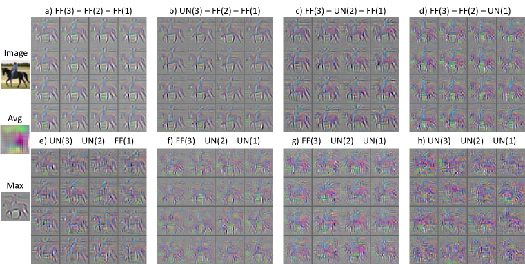
Despite the stochastic nature of the model, the multinomial distributions effectively capture the regularities of the data. To demonstrate this, we compare the outputs produced by a deconvolutional network when sampling using the feedforward (FF) proabilities versus sampling from uniform (UN) distributions. In contrast to Fig. 6(a) which uses only feedforward proabilities, Fig. 6(b-h) replace one or more of the pooling layers’ distributions with uniform distributions. The feed forward probabilities encode significant structural information, especially in the lower layers of the model. Additional visualizations and videos of the sampling process are provided as supplementary material at www.matthewzeiler.com/pubs/iclr2013/.
5 Discussion
We propose a simple and effective stochastic pooling strategy that can be combined with any other forms of regularization such as weight decay, dropout, data augmentation, etc. to prevent over-fitting when training deep convolutional networks. The method is also intuitive, selecting from information the network is already providing, as opposed to methods such as dropout which throw information away. We show state-of-the-art performance on numerous datasets, when comparing to other approaches that do not employ data augmentation. Furthermore, our method has negligible computational overhead and no hyper-parameters to tune, thus can be swapped into to any existing convolutional network architecture.
References
- [1] D. C. Cireşan, U. Meier, J. Masci, L. M. Gambardella, and J. Schmidhuber. Flexible, high performance convolutional neural networks for image classification. In IJCAI, 2011.
- [2] G.E. Hinton, N. Srivastave, A. Krizhevsky, I. Sutskever, and R. R. Salakhutdinov. Improving neural networks by preventing co-adaptation of feature detectors. arXiv:1207.0580, 2012.
- [3] K. Jarrett, K. Kavukcuoglu, M. Ranzato, and Y. LeCun. What is the best multi-stage architecture for object recognition? In ICCV, 2009.
- [4] Y. Jia and C. Huang. Beyond spatial pyramids: Receptive field learning for pooled image features. In NIPS Workshops, 2011.
- [5] A. Krizhevsky. Learning multiple layers of featurs from tiny images. Technical Report TR-2009, University of Toronto, 2009.
- [6] A. Krizhevsky. cuda-convnet. http://code.google.com/p/cuda-convnet/, 2012.
- [7] Y. LeCun. The MNIST database. http://yann.lecun.com/exdb/mnist/, 2012.
- [8] Y. LeCun, L. Bottou, Y. Bengio, and P. Haffner. Gradient-based learning applied to document recognition. Proceedings of the IEEE, 86(11):2278–2324, 1998.
- [9] G. Montavon, G. Orr, and K.-R. Muller, editors. Neural Networks: Tricks of the Trade. Springer, San Francisco, 2012.
- [10] V. Nair and G.E. Hinton. Rectified linear units improve restricted boltzmann machines. In ICML, 2010.
- [11] Y. Netzer, T. Wang, A. Coates, A. Bissacco, B. Wu, and A. Y. Ng. Reading digits in natural images with unsupervised feature learning. In NIPS Workshop, 2011.
- [12] P. Sermanet, S. Chintala, and Y. LeCun. Convolutional neural networks applied to house numbers digit classification. In ICPR, 2012.
- [13] P. Simard, D. Steinkraus, and J. Platt. Best practices for convolutional neural networks applied to visual document analysis. In ICDAR, 2003.
- [14] http://gp-you.org/. GPUmat. http://sourceforge.net/projects/gpumat/, 2012.
- [15] M. Zeiler, G. Taylor, and R. Fergus. Adaptive deconvolutional networks for mid and high level feature learning. In ICCV, 2011.