Measurement of Baryon Acoustic Oscillations in the Lyman- Forest Fluctuations in BOSS Data Release 9
Abstract
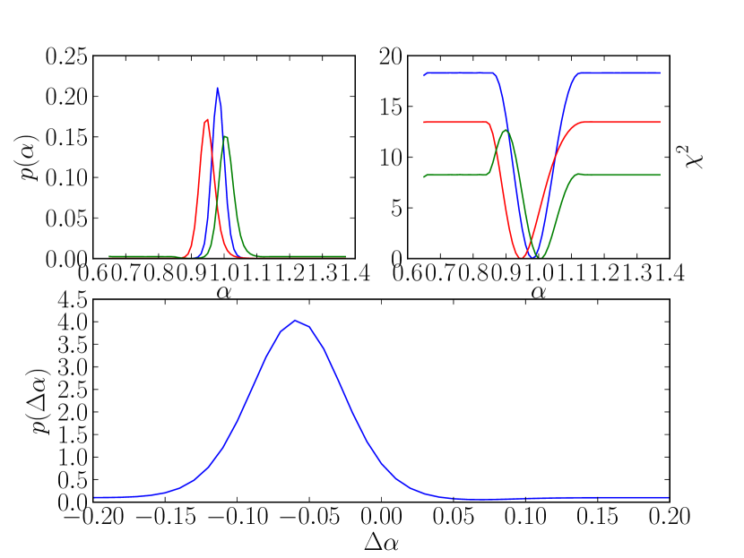
We use the Baryon Oscillation Spectroscopic Survey (BOSS) Data Release 9 (DR9) to detect and measure the position of the Baryonic Acoustic Oscillation (BAO) feature in the three-dimensional correlation function in the Lyman- forest flux fluctuations at a redshift . The feature is clearly detected at significance between 3 and 5 sigma (depending on the broadband model and method of error covariance matrix estimation) and is consistent with predictions of the standard CDM model. We assess the biases in our method, stability of the error covariance matrix and possible systematic effects. We fit the resulting correlation function with several models that decouple the broadband and acoustic scale information. For an isotropic dilation factor, we measure (stat.) (syst.) (multiple statistical errors denote 1,2 and 3 sigma confidence limits) with respect to the acoustic scale in the fiducial cosmological model (flat CDM with , ). When fitting separately for the radial and transversal dilation factors we find marginalised constraints (stat.) (syst.) and (stat.) (syst.). The dilation factor measurements are significantly correlated with cross-correlation coefficient of . Errors become significantly non-Gaussian for deviations over standard deviations from best fit value. Because of the data cuts and analysis method, these measurements give tighter constraints than a previous BAO analysis of the BOSS DR9 Lyman- forest sample, providing an important consistency test of the standard cosmological model in a new redshift regime.
1 Introduction
Discovery of the accelerated expansion of the Universe at the end of 20th century was one of the largest surprises in cosmology [1, 2]. Since then, much effort has gone into measuring the properties of the dark energy that is believed to drive the acceleration of the Universe using a variety of techniques (see extensive review [3] and references therein). Measurements that directly probe the expansion history of the Universe reveal how the energy density of its constitutive components changes with expansion and thus allow inferences to be made about their nature. The two important techniques in this field are the type Ia supernovae (SN Ia) and baryonic acoustic oscillations (BAO) [4, 5, 6, 7, 8, 9]. The former rely on the fact that SNIa are standarizable candles. Measuring supernovae fluxes and redshifts thus provide information about the luminosity distance as a function of redshift. The BAO technique, which is the focus of this paper, relies on the fact that the baryonic features in the correlation properties of tracers of the large scale structure of the Universe can act as a comoving standard ruler.
BAO are acoustic oscillations in the primordial plasma before decoupling of the baryonic matter and radiation. These oscillations imprinted a characteristic scale into the correlation properties of dark matter, which exhibit themselves as a distinct oscillatory pattern in the power spectrum of fluctuations or equivalently a characteristic peak in the correlation function. The scales involved are large ( Mpc) so the feature remains in the weakly non-linear regime even today. Any tracer of the large-scale structure can measure this feature and use it as a standard ruler to infer the distance to the tracer in question (when the ruler is used transversely) or the expansion rate (when the ruler is used radially).
The main attraction of BAO technique is that one is measuring the position of a peak and that many systematic effects are blind about the preferred scale and thus influence the two-point function only in broadband sense. Such systematic effects can be efficiently marginalized out with little or no signal loss. The caveat in the case of the Lyman- forest analysis is that systematic effects that appear at certain pairs of wavelengths can produce a peak-like feature in the correlation function in the radial direction.
Traditionally, the tracer used to measure BAO consisted of galaxies, and measuring BAO with galaxies is a mature method [8, 9]. However, the current measurements of the BAO with galaxies are restricted to redshifts , due to difficulty in measuring redshifts of sufficient numbers of objects efficiently. Even the proposed future BAO projects such as BigBOSS [10] will measure the BAO only to redshifts of less than using galaxies as a tracer of cosmic structure. However, there is strong scientific motivation for measuring the expansion history of the Universe at higher redshifts. Dark energy suffers from many tuning problems that can be alleviated by introducing an early dark energy component [11, 12, 13, 14, 15, 16]. Such a component can only be measured by a technique sensitive to the expansion history at high redshift. In this paper we present such a measurement using the Lyman- forest as a tracer of dark-matter fluctuations at .
This “Lyman- forest ” denotes the absorption features in the spectra of distant quasars blue-ward of the Lyman- emission line [17]. These features arise because the light from a quasar is resonantly scattered by the presence of neutral hydrogen in the intergalactic medium. Since the quasar light is constantly red-shifting, hydrogen at different redshifts absorb at different observed wavelength in the quasar spectrum. The amount of scattering reflects the local density of neutral hydrogen. Neutral hydrogen is believed to be in photo-ionization equilibrium and therefore the transmitted flux fraction at position is given by [18]
| (1.1) |
where is optical depth for Lyman- absorption at position . This optical depth scales roughly as a power law in the baryon over-density . The coefficient would be two for an idealized two-body process, but is in practice closer to due to the temperature dependence of the recombination rate. The Lyman- forest thus measures some highly non-linear but at the same time very local transformation of the density field. Any such tracer will, on sufficiently large scales, trace the underlying dark matter field in the observed redshift-space as
| (1.2) |
where are the flux and matter over-densities in Fourier space respectively and is the matter over-density in the Fourier space. The quantity is the cosine of the angle of a vector with respect to the line of sight and the parameter is the logarithmic growth factor. In the peak-background split picture, the two bias parameters can be derived as a response of the smoothed transmitted flux fraction field to a large scale change in either overdensity or peculiar velocity gradient [19]:
| (1.3) | |||||
| (1.4) |
Both bias parameters ( and ) can in principle, be determined from numerical simulations of the intergalactic medium, but they can also be determined from the data as free parameters to be fit. The dimensionless redshift-space distortion parameter determines the strength of distortions [20]. Conservation of the number of galaxies requires that in that case and hence is completely specified by the value of and density bias . Unfortunately, there is no such conservation law for transmitted flux fraction and hence the two parameters are truly independent for the Lyman- forest 2-point function. In the rest of this paper we will work with density bias parameter and redshift-space distortion parameter and treat them as free parameters to be constrained by the data.
Numerical simulations have shown that for plausible scenarios, the Lyman- forest is well in the linear biasing regime of equation (1.2) at scales relevant for BAO. Fluctuations in the radiation field can, if sufficiently large, invalidate the equation (1.2), but it has been shown that these variations are unlikely to produce a sharp feature that could be mistaken for the acoustic feature [21, 22]. Therefore, measuring three-dimensional (3D) correlations in the flux fluctuations of the Lyman- forest provides an accurate method for detecting BAO correlations [23, 24, 25].
Using the Lyman- forest to measure the 3D structure of the Universe became possible with the advent of the Baryonic Oscillation Spectroscopic Survey (BOSS, [26, 27]), a part of the Sloan Digital Sky Survey III (SDSS-III) experiment [28, 29, 30, 31, 32, 33]. This survey was the first to have a sufficiently high density of quasars to measure correlations on truly cosmological scales [34]. This paper was also first to point out difficulties in measuring the large-scale fluctuations in the Lyman- forest data; and many design decisions in this paper were chosen to alleviate them. The BAO in the Lyman- forest was first detected in [35] using the same dataset as this work. They found a dilation scale . Both works were done within the same working group in the BOSS collaboration, but use different and an independently developed pipelines. We assess these differences more thoroughly in Section 5.4. We refer the reader to these publications for a more thorough review of the Lyman- forest physics and the BOSS experiment.
This paper is focused on the methodology and results of measuring the 3D correlation function from the flux transmission fluctuations. The companion paper [36] focuses on the methodology of constraining the BAO parameters. The final results on the BAO parameters are presented in this paper.
This paper is dedicated purely to detecting the BAO feature in the correlation function of Lyman- forest fluctuations as measured by BOSS Data Release 9 [37]. We do not attempt to provide robust measurements of bias and parameters; we therefore adopt aggressive inclusion of data that is tuned to maximize the likelihood of a significant BAO peak detection. We stress that in the early stages of analysis, the peak between 100-130 was blinded and these cuts were decided on and fixed before “opening the box”. No cuts were changed after that, but the data analysis code has been improved.
The paper is structured as follows. In section 2 we describe our data samples and basic selection criteria. In section 3 we explain the complicated process of measuring the 3D correlation function using an optimal estimator, its errors and biases, while presenting intermediate results. Section 5 discusses application of the method to the real and synthetic data and discusses potential errors. Finally, we convert our many noisy measurements into a plot of the BAO bump in Section 6. We conclude in Section 7. The mathematical details of optimal estimators are elaborated in Appendices.
2 Instrument, Data & Synthetic data
2.1 DR9Q Sample
In this work we use BOSS quasars from the Data Release 9 (DR9, [37]) sample in order to facilitate reproducibility by outside investigators. The quasar target selection for the DR9 sample of BOSS observations is described in detail in [38] and [39]. A similar dataset is released in [40] including continua for normalization and default recommendations for data masking.
The main approach in this work has been to aggressively use as much data as possible, to maximize the likelihood of a significant detection of the BAO peak and the accuracy of the determination of its position. The argument that we are making, and which underpins the robustness of many BAO measurements, is that systematic effects that affect the measured two-point statistics will in general produce a broadband contribution and thus not affect the position of the peak itself, since broadband contributions are marginalized out in the process of fitting the BAO position. At the same time, however, adding poorly understood data might lead to an increase in the noise that might outweigh the benefit of additional information. We settled on a set of cuts described below.
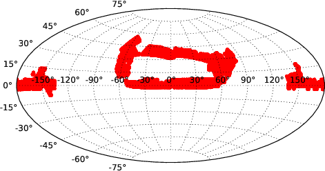
We select quasars from the DR9Q version of the Value Added Catalog (VAC) of the French Participation Group (FPG) visual inspections of the BOSS spectra [41]. The position of the quasars on the sky is plotted in figure 1. The total number of quasars in our analysis after the cuts performed below is 58,227. The covered area is optimized through survey strategy considerations and will become more uniform as the survey approaches completion in 2014.
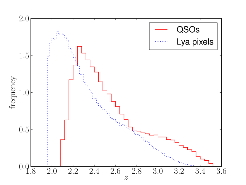
We limit our analysis to quasars with redshifts . Throughout this work we use the visual redshifts (Z_VI) from the DR9Q. The low number density of quasars at redshifts larger than 3.5 renders them not useful for measuring the BAO signal, which is the main goal of this paper. We show the distribution of quasar redshifts and the Lyman- forest pixels in Figure 2.
For repeated observations of a given object the DR9Q catalog contains all the listed observations, as well as the observation deemed to be optimal. We performed the analysis either by restricting the sample to the subset of best observations as well as using all observations. In the latter case, we simply co-add the observations on the nearest pixel point using the pipeline-reported inverse variances. We do not use the noise correction (discussed later) when performing this co-add, but since the correction is a function of wavelength it would rescale all contributions equally and thus have no effect when stacking in observed wavelength.
We apply several cuts to the data. First, we treat quasars that are considered Broad Absorption Line (BAL) quasars differently. The DR9Q catalog contains a measured value of balnicity index [42]. We remove quasars with km/s. We additionally drop quasars that DR9Q visual inspection flagged as highly unusual ().
Second, we mask regions around bright sky lines. The mask is obtained by the following procedure: We subtract the sky model from the sky fibers. The model’s prediction at the position of the sky fiber does not match the spectrum of the sky fiber, since the model fits a smooth polynomial model over all sky fibers and thus sky subtracted sky fibers do not have zero flux. We stack all sky-subtracted sky fibers and measure the root mean square defined over standard BOSS pixels () boxcar of this stack. Next we mask all pixels that exceed this r.m.s. by a factor of 1.25. The masked pixels are excluded from the r.m.s. measurement and the process is iterated until the mask converges. This mask excludes very few pixels in the blue end of spectrograph, simply because there are not many sky-line in that wavelength region.
Third, we exclude portions of the data affected by the Damped Lyman- (DLA) systems using the so-called concordance DLA sample [43]. Briefly, this dataset was established by three groups within the BOSS Lyman- forest working group, two of which developed algorithms for detecting DLAs in data automatically and the third inspected all quasars visually. All three groups have provided catalogs of systems. One of these three samples is published in [44]. The concordance catalog DLAs were identified by at least two of the three groups. We do not use data within 1.5 equivalent widths from the center of a DLA.
When measuring the correlation in the Lyman- forest, we use a wide region of the forest, spanning - Å for most quasars and - Å for the remaining BAL quasars (). We also exclude pixels with observed wavelength less than Å, beyond which the signal-to-noise of the spectrograph and spectro-photometric calibration become very poor.
We assume that the measurement noise does not correlate between pixels, but we apply a correction to the BOSS spectral extraction pipeline estimates of the noise. To derive this correction, we fit a cubic polynomial to the smooth region of quasar spectra between rest-frame 1420 and 1510 Å and compared the fit residuals with the pipeline error estimates. We find that the co-added spectra have an observer-frame wavelength dependent mis-estimation of the noise, which follows the square root of the ratio of pixel sizes between the co-added and individual exposure spectra. This value is a under-estimate of the noise variance below observer-frame 4750 Å and a over-estimate above 4750 Å; this correction is not valid beyond 6000 Å where both arms of the BOSS spectrograph contribute to the spectrum. We correct for this mis-calibration by adjusting the pipeline noise by the square root of the co-add-to-individual exposure pixel size ratio.
2.2 Synthetic data
Data analysis procedures in this work were tested on the synthetic data that was generated in nearly the same manner as for the previous work [34] and we briefly review it here for completeness.
We want to generate a transmitted flux-field with desired two-point function and approximately correct probability distribution function. For a general transformation , where is a Gaussian auxiliary field, the 2-point correlation functions of the flux field, , and that of the auxiliary Gaussian field, , can be related by
| (2.1) |
We assume that is log-normally distributed so that specifying the mean transmitted flux fraction , in addition to the desired target power spectrum completely specifies the required properties of the auxiliary Gaussian field. This inversion is done numerically. The Gaussian field is initially generated assuming parallel Lyman- forest lines of sight and stationary (non-evolving) field: the effects of non-parallel lines of sight and field evolution are then obtained by interpolating between redshifts. The assumption of parallel lines of sight and stationary fields significantly simplifies the problem. Decomposing the line of sight flux fluctuations of a quasar into its Fourier components , the cross-correlation vanishes for different Fourier modes:
| (2.2) |
This allows one to generate the field one parallel Fourier mode at a time. For each such-mode, one thus needs to generate a correlated Gaussian field vector of the size , where is the number of quasars. We perform this using standard methods for generating correlated Gaussian fields with a desired covariance matrix by Cholesky decomposing the matrix and multiplying with a vector of uncorrelated unit-variance Gaussian field. Technical aspects of synthethic data generation and tests that demonstrate the validity of the generated fields are described in great detail in [45].
Our present implementation of synthethic data generation is still numerically extremely demanding. To be able to generate a full synethetic dataset, we split it into four geometrically self-contained “chunks”, ignoring correlations across chunk borders. We have tested explicitly that this approximation introduces no bias. We have thus generated fifteeen synthethic realizations of our dataset. These synethetic datasets were also used in [35].
Compared to [34], mock data were created using slightly different bias parameters and . There were made more realistic in this work by adding several effects that are present in the spectrograph and were not accounted for in the previous work. We add noise to the mocks based upon an object-by-object fit to the observed photon noise in the real data. We then generate a noisy and mis-calibrated estimate of the true noise to model the pipeline reported noise and use that noise to generate a noise realization for the analysis. The mock spectra fluxes were multiplied by a polynomial in to match the real data to simulate QSO flux mis-calibration and a small amount of sky spectrum is added to model a sky subtraction bias in the BOSS data. These additions will be described in greater detail in a future publication [46]. In one respect, the synthetic data were less realistic that the similar synthetic datasets used in [34], namely, we did not contaminate the data with associated forest metals in this work.
3 Data Analysis
In this section we describe the steps taken in the data analysis. The same procedure is adopted both to the real and the synthetic data described in section 2.2.
The overview of data analysis is as follows:
-
•
Continuum fitting. (Section 3.1) First we perform the basic continuum fitting, where the pixels are treated as independent. Continuum fitting can be described as a process of fitting a model for what the spectrum of a given quasar would look like in a completely homogeneous universe, i.e. there would be no forest, except the mean hydrogen absorption. We fit for the mean continuum, the redshift dependence of the mean transmission in the forest and the intrinsic variance including its redshift dependence. We also fit for the per-quasar amplitude and slope across the forest.
-
•
One-dimensional Pixel Power Spectrum measurement. (Section 3.2) In the second step we generalize the variance in the pixels to the full one-dimensional (1D) power spectrum of flux fluctuations as a function of redshift. We refit the individual quasar forest amplitudes and effective spectral slopes, the mean transmission as a function of redshift and the effective 1D power spectrum. This power spectrum is not appropriate for cosmological analysis, as it does not deconvolve the instrument PSF and the instrument noise is treated coarsely. This co-variance is only required for the weighting in the measurement of the 3D correlation function.
-
•
Estimation of the three-dimensional correlation function and its covariance matrix. (Section 3.3) The next step is estimation of the 3D correlation function. This is done by weighting quasar data with a per-quasar inverse covariance matrix and performing optimal quadratic estimation of the correlation function. This analysis is done in a coordinate system that is composed exclusively of observable quantities, i.e. difference in logarithm of the observed wavelength, angular separations on sky and the pixel pair redshift (which is just a proxy for the mean redshift of a given pixel pair). We use several methods to estimate the covariance matrix coming from the optimal estimator.
-
•
Estimation of BAO position and significance. (Section 4) Finally, we measure the position of the BAO peak from the measured 3D correlation function. The uncertainties on the BAO parameters of interest using different covariance matrices and broadband models.
3.1 Continuum fitting
A reasonably general model of the observed flux can be written as follows
| (3.1) |
Here we use the index to denote a particular quasar (probing a direction on the sky), is the observed wavelength and is the rest-frame wavelength of the quasar. Since hydrogen absorbing through Lyman- at redshift produces a decrement at observed , we can use interchangeably with absorption redshift. The term denotes convolution, i.e., smoothing by the point-spread function of the spectrograph and the final term in equation (3.1) is the spectrograph noise contribution. The pipeline provides an estimate of the pixel noise under the assumption that it is independent from pixel to pixel (but we correct for this as described earlier).
The mean unabsorbed quasar spectrum, also referred to as the continuum, is given by and we absorb the diversity in both the quasar amplitude and quasar shape into . In this work, we model as linear function of
| (3.2) |
where and are the highest and lowest wavelengths in the forest.
The term in Equation 3.1 is the mean quasar transmission in the forest and can be distinguished from the residual variations in the spectrograph transmissivity, , by the virtue that the former is unity outside the forest. Finally, the term describes an additive systematic component, likely to be dominated by the sky. The term inside brackets are the fluctuations in the transmission, whose correlation properties we are attempting to infer from the data.
With expediency in mind, we make several simplifying assumptions. First, we ignore the point-spread function of the spectrograph, since it affects exclusively small scales and can be completely neglected for purely 3D analysis. Second, we set the sky contribution and the spectrograph transmissivity . This choice means that and are really just parametrization of continuum model under the assumption that it is factorisable as after the individual quasar mean luminosity and spectral slope have been fitted (Equation (3.2)). The fitted will also absorb the contribution from the variation of spectrograph properties as a function of wavelength which have not properly been calibrated by the pipeline.
Finally, in the initial parts of the fitting process, we model fluctuations as Gaussian and uncorrelated. Therefore, our likelihood model in the first step of continuum fitting can be written as
| (3.3) |
where the sum is over all forest pixels in all quasars, denotes the intrinsic variance of the flux transmissions (i.e., variance in the cosmological field) and the pipeline noise.
We measure two amplitude parameters for each quasar ( and , defining amplitude and slope), in 95 bins between Å and Å and further 167 bins extending to Å. The intrinsic variance and are measured in 16 bins between redshifts and (linearly interpolating between bins for the case of ).
This approach contains a considerable number of parameters. We maximize the likelihood by brute-force maximization, employing a Newton-Raphson algorithm with numerical derivatives. We do not attempt to derive errors on these parameters as these errors will not dominate the errors on the final quantities that we are attempting to derive.
To gracefully approach a good solution, we start by fitting just , , intrinsic variances and constant amplitudes across rest wavelength Å. Next we focus on the forest region and refit individual amplitudes and slopes together with refitting variances. As a third step we refit variances and slopes together with measuring the 1D power spectrum as described in the next section.
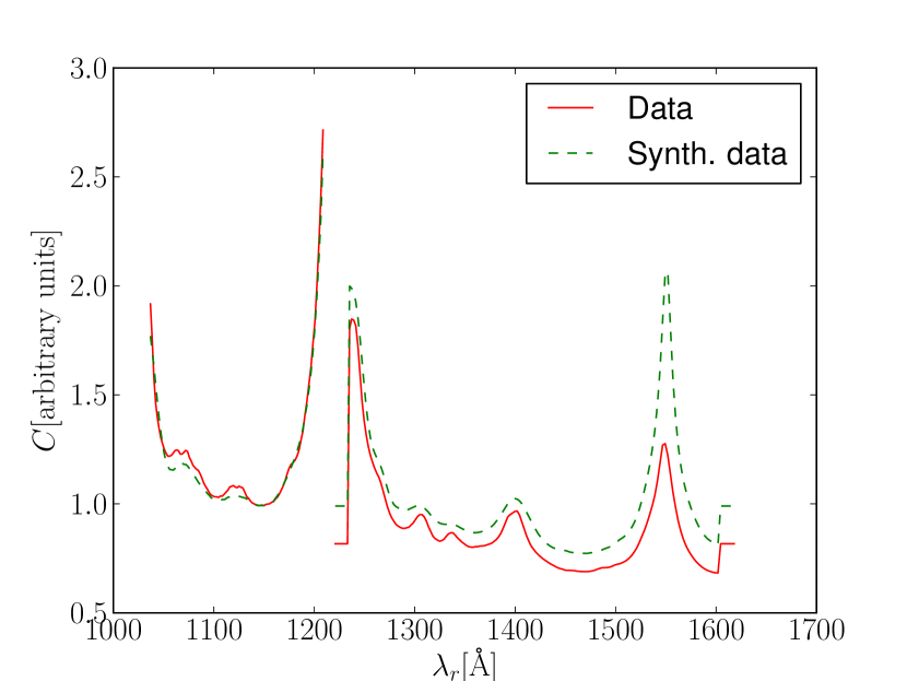
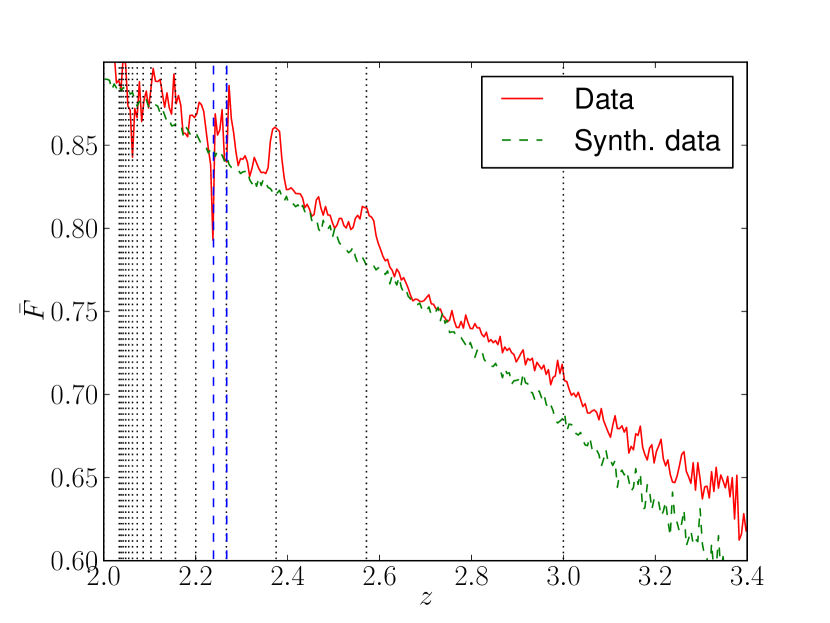
Figures 3 and 4 show the mean continuum and for data and synthetic data. The measurement of shows the expected structure: there is more absorption at higher redshifts. However, we also see structure at the position of rest-frame Balmer lines. This structure is an artifact of the pipeline and arises due to imperfect interpolation of masked Balmer regions in the calibration stars. These features are essentially completely absorbed into and we do not see any residual structure associated with Balmer lines in other tests. We also see features at the positions of CaH and CaK absorptions.
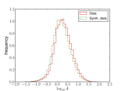
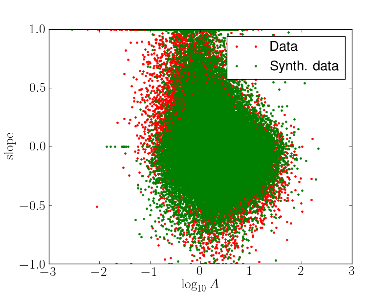
In Figure 5 we show the distribution of amplitudes and effective spectral slopes as fitted to the data and to the synthetic data. The histogram of amplitudes for the data matches that of the synthetic data very well. This result arises essentially by construction, since our synthetic quasars are matched in flux to real quasars. The right-hand panel considers the spectral slope. The slope is defined so that it is if any one of the two individual fitted amplitudes at two wavelengths is zero. We fit for the slope at two fixed observed wavelengths at the edge of the forest even though there might be no data at those edges. Therefore the amplitude measurement can be quite uncertain and produce a value outside a physically acceptable range. In general, the diversity of spectra in synthetic data is a good representation of that in real data, although, as expected the real data are slightly more diverse.
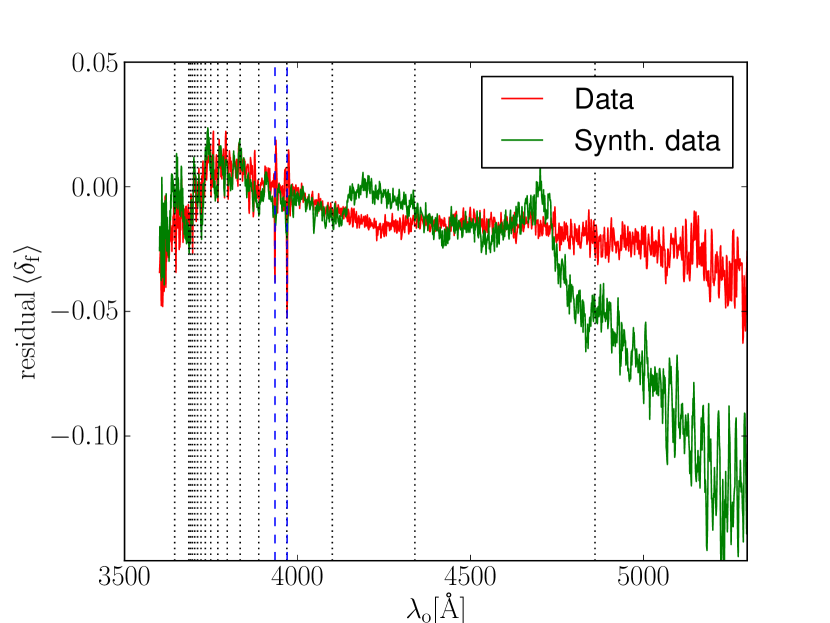
Our model for the continuum in Equation 3.1 is not perfect and there will be systematic residuals between true and our estimates in addition to noise. A useful check for these residuals is to stack our estimates of in bins of observed wavelength (or redshift): for unbiased estimates these should vanish, but in practice this is not exactly the case. In Figure 6 we show the residuals from our continuum fitting which are obtained by an inverse covariance weighted average of all data in bins of observed wavelength. These residuals are removed from the data before measuring the 3D correlation function, but they essentially imply a calibration uncertainty on the final correlation function of a couple of percent (although this is irrelevant for BAO fits). Since we are fitting for the amplitude of quasars in flux and then dividing by a noisy estimate to derive , we expect that the mean of will not be zero (essentially because ). We also notice that these residuals are considerably worse for the synthetic data. This result arises partially because the synthetic data is somewhat noisier, especially at higher redshift (see the next section) and partially because addition of some systematic effects in the synthetic data might be introducing more contamination than exists in the real data. Most importantly, however, we see no effects of structure at the position of Balmer lines, indicating that these features are nearly perfectly removed with the fit. The caveat is, of course, that one could have structure associated with Balmer features that would be, for example, correlated from plate to plate and produce contaminating signal while still averaging to zero. This concern is discussed further in Section 5.2.
3.2 One-dimensional Pixel Power Spectrum measurement
As the final step in the continuum fitting process, we measure the 1D power spectrum of pixels. This power spectrum enables a nearly optimal weighting to be used when measuring the 3D two-point function. This step essentially generalizes the model of the covariance of the flux transmission from uncorrelated pixels to pixels correlated across a single quasar.
| (3.4) |
In practice, we measure the power spectrum in flat power bands in (i.e., the 1D power spectrum is approximated as a set of top-hat bins) and interpolated in redshift. For any pair of pixels, the effective redshift is taken to be given by the geometrical mean of of two pixels (or equivalently geometrical mean of their or mean of their ). The distance is measured in converted to the standard units of (by multiplying by speed of light). The integral of flat power band can be trivially calculated analytically.
To estimate the 1D power spectrum we use the standard optimal quadratic estimator [47, 48, 49] and has been applied to Lyman- forest data in before in [50]. The formalism behind optimal quadratic estimators generalizes the signal-to-noise weighting of the data from scalar weights proportional to the inverse variance applied to each data-point individually, to multiplying the entire data-vector by the inverse of the covariance matrix. Optimal quadratic estimator methodology can improve the signal-to-noise of the measurement and provides good (but not perfect) error-estimates. We review the methodology in the Appendix A.
We measure the 1D power spectrum in 20 bins logarithmically spaced between (center of the first bin) and (center of the last bin) in steps of dex and 9 bins in redshift, uniformly spaced between and . Although we have very few pixels with , they contribute to the power spectrum measurements extrapolated to the bin (to keep the binning in redshift uniform). This results in 180 1D power spectrum overall bins. The lower range for the lowest -bin is extended to .
We do not attempt to deconvolve the point spread function or carefully understand the effect of noise – we are only attempting to estimate the correct pixel-pixel correlations to use in weighting in the 3D correlation estimation. For example, if noise is underestimated, then one measures a power spectrum that has a constant offset with respect to the true power spectrum, but the total signal-plus-noise power will remain unchanged. The same is true for the effect of the point-spread function. If we deconvolved the effect of the PSF, we would be putting exactly the same PSF back into the correlation matrix when making a prediction for the covariance matrix of a single quasar forest. In summary, in this paper, the 1D power spectrum is treated as an intermediate product used for weighting the 3D two-point function estimate and is not intended to be useful as a measurement of the physical 1D Lyman- forest power spectrum. Any error in 1D power spectrum results in a less-optimal 3D weighting, but will not bias the 3D measurement.
When measuring the 1D power spectrum, we iterate between measuring the 1D power spectrum and refitting all per-quasar amplitude and slope parameters. The process converges in approximately five iterations. When measuring the 1D power spectrum we consistently marginalize out modes that were fitted by the continuum fitting as described in Appendix B and discussed later.
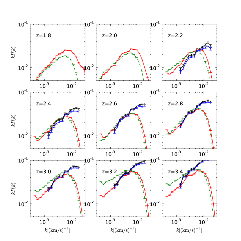
In Figure 7 we plot the 1D power spectra for real and synthetic data. The data and the synthetic data show a good overall agreement, although they differ considerably in the high redshift bins. The edge redshifts are essentially extrapolations from the measured data and should not be taken too seriously. In addition, the data in the highest redshift bins come from the region close to the quasar (we use data all the way to Å and do not use quasars with ). Finally, in this work we use only a rough correction for the pipeline mis-estimation of the noise, which can be thought of as a constant additive uncertainty for the data. The errors reported by the synthetic datasets are biased (on purpose, to model the pipeline errors) which we did not attempt to correct, so it is natural that the synthetic data will not measure just the intrinsic power spectrum. However, when doing inverse covariance weighting for the 3D measurement, the relevant quantity is the sum of noise and intrinsic power, so noise mis-estimation will result in extra (or less) intrinsic power, but will affect the sum only at second order. We also plot the measured values from [50], which have been corrected for the effect of resolution and thus do not show the beam suppression at high values. The wiggles in the measured power spectra due to presence of Si III are clear in both our dataset and [50] power spectra, while absent from the synthetic data.
3.3 Quasi-optimal estimation of the three-dimensional correlation function
Once the 1D correlation properties of quasars are measured, we proceed to measure the 3D correlation function.
As in the case 1D power spectrum measurement, we use the optimal quadratic estimator. Applying the estimator blindly would involve inverting matrix the size of the number of pixels. Since this is numerically prohibitive, we instead approximate it as a block-diagonal matrix, where each block corresponds to a single quasars. In other words, for the purpose of data-weighting, we assume quasars to be uncorrelated. This approach is optimal in the limit of small cross-correlations between neighbouring quasars. Technical details are outlined in the Appendix A, in particular, we numerically implement equations A.17, A.18 and A.19. This approach is always unbiased, but the resulting error-covariance matrix will ignore contributions to the error covariance matrix stemming from correlations between pixels in neighboring quasar pairs.
We never measure the 3D correlations using pixel-pairs that reside in the same quasar since continuum fitting errors are expected to be correlated within the same quasars, but significantly suppressed across quasars (true quasar continua are thought to be completely uncorrelated across quasars111A notable exception are systems with multiply lensed quasars.). We sort pairs of quasars into SDSS plates. If a given quasar pair has two objects observed on two different plates, the pair is uniquely associated with one of the two plates. There are 817 plates in DR9 which parcels the problem of computing the 3D correlation function into feasible computation chunks, but also allows a suitable base for bootstrapping errors. In particular, one could imagine a class of systematic errors that are associated with plates and such errors would be “discovered” as extra variance by the bootstrap algorithm.
However, even in the approximation where quasars are decoupled, the computation of estimates is still too slow. Therefore, we reduce the problem by optimally reducing the number of pixels by a factor of three or four. This reduction is done after multiplying the data vector by the inverse covariance matrix as described in Appendix C.
Our model for the 3D correlation function is parametrized in terms of completely observable coordinates that do not assume a fiducial cosmology. In particular, each bin of the measured correlation function is characterized by the radial separation measured in (where is the observed wavelength of a given pixel), angular separation measured in radians and redshift (which is just a proxy for the mean observed wavelength). In our parametrized model for the correlation function that we measure, we interpolate linearly in and . This is particularly important in the redshift direction, where bins are quite wide. In the angular direction, however, the bins are assumed to be uncoupled (i.e.,top hat in shape). The reason for this choice is that it significantly simplifies the resulting Fisher matrix, which is zero for elements corresponding to pairs of estimates at different separations. This point will be elaborated upon further in Section 3.5.2.
The main advantage of this approach is that one is truly measuring correlations without an assumption on cosmology. The main drawback is the large number of correlation bins and an inevitable smoothing of the measured correlation function, because the BAO peak position in configuration space is a function of redshift. We will show later that this is a negligible effect. We use three redshift bins (, and ), 18 separation bins centered around 5,15,…175 arc minutes and 28 bins in spanning the relevant range with non-uniform bin spacing (0, 0.001, 0.003, 0.005 …0.049, 0.059, 0.083); this procedure results in 1512 measured bins.
The quadratic estimator does produce a Fisher matrix as an estimate of error covariance of the measured data-points. In our case, this assumes that the flux fluctuations correlation within individual quasars dominate the covariance matrix. In practice we would like to have a more robust measurement of the error-bars for our final measurement; for this purpose we use various techniques that estimate the covariances internally.
3.4 Distortion of the three-dimensional correlation function
It has been known since the 1970s [51] that the naïve estimates of 3D correlations from the Lyman- forest result in distorted correlation function due to continuum fitting.
The effect appears because continuum fitting inevitably entails inferring information about continuum shape from the actual forest data and the model will naturally try to minimize the variance of residuals with respect to the predicted mean continuum. For example, an unbiased estimates of will have a small but finite mean due to presence of Fourier mode whose wavelength is much larger than then the length of the forest. Continuum fitting cannot distinguish between a true underlying offset and a change in quasar amplitude and will typically set the amplitude of such mode to zero. The size of this effect is surprisingly large and will result in a biased correlation function measurement.
In this work, we would, in principle, not need to worry about distortion effects, because we are trying to find an isolated bump in the correlation function, while distortion is a smooth function that could be absorbed with a sufficiently flexible broadband. Nevertheless, prevention is always preferable to cure.
There are several ways to address this distortion. The simplest one, used in [34], is to assume that the effect of continuum fitting is to force a set of measured values to have zero mean in each quasar line of sight, by subtracting its mean . One can propagate this assumption through a simple analytical model and obtain a formula for the correction. Resulting expression is approximate, but worked well for the signal-to-noise used in the above paper. In this work we can do better than that by removing the effect of the continuum fitting by down-weighting linear combinations of datapoints that we know are affected by the continuum fitting process, namely the constant offset and slope in per-quasar data-vectors. This is done by associating large variances with these particular modes as described in Appendix B. This technique is equivalent to discarding a point by associating a very large variance with it, only that we now associate a large variance with a particular linear combination of points. Of course, the contribution from a particular linear combination can only be down-weighted if one uses matrix weighting. The result is that, by construction, these marginalized modes cannot have an effect on the final result.
In particular, we marginalize modes that appear as a constant offset and those that appear as a linear function of in the field. We add these terms to the covariance matrix both for the 1D P(k) measurements as well as the 3D correlation function..
As a result of this marginalization, the estimator propagates the uncertainty associated with the unknown modes into the measurements of the 3D correlation function. As an unfortunate consequence of working in configuration space, this approach results in large, but nearly completely correlated errors in measurements. In Fourier space, this result corresponds to a few poorly measured low- modes.
For plotting purposes, these modes can be self-consistently projected out of the measured correlation function and theory predictions, resulting in a distorted correlation function measurement whose error-covariance is considerably more diagonal as we will do in the Section 6. However, the shape of the distortion is now known from the eigen-vectors of the projected modes. If one limits the analysis to inspection of values, this is, of course, unnecessary.
3.5 Determining the covariance matrix of the measurements
There are two aspects of any analysis that can affect the results in a detrimental way: the bias of the estimation procedure and the uncertainty in the derivation of the covariance matrix of the errors. The former can be most precisely determined by examining the results on the synthetic data. As far as accuracy of the covariance matrix is concerned, fifteen realizations is not enough if one wants to consider events that are rarer than in (i.e., events). Therefore one must rely on the internal checks of the data, and we provide several such methods.
3.5.1 Bootstrapped covariance matrix
We start by creating a bootstrapped covariance matrix. This process recreates bootstrap “realizations” of the data by randomly selecting, with replacement, plates from the original set of plates and combining them using their estimator provided weights. In each realizations some plates appear more than once and sometimes never. The covariance matrix of these realizations can be assumed to be a good approximation to the covariance of the estimation, if the plates are sufficiently independent and if we have sufficient number of them. Although the plates are not strictly independent (the pairs of quasars spanning two plates are randomly assigned to one of the plates), the approximation that these are independent should be a very good one - as we will see later, not just plates, but even quasars can be considered independent. There is one subtlety, however. The variance associated with the distortion of the correlation function described in Section 3.4 will not be accurately represented in this bootstrapped matrix, because this variance will be artificially low (by virtue of these modes being calibrated out) and therefore the bootstrapped matrix cannot be used directly on the measured correlation function.
The full bootstrapped covariance matrix from the dataset (or one realization of the synthetic data) is non-positive definite, because its size is while the number of plates contributing to the bootstrapped matrix is only 817. In other words, the 817 vectors do not span the full 1512 dimensional space and therefore linear combinations of them cannot generate 1512 independent eigen-vectors of the covariance matrix. However, the bootstrapped covariance matrix where elements corresponding to different angular separations are assumed independent is positive-definite as we are now determining eighteen matrices from eighteen sets of 817 vectors of size . We show that this approach is a good approximation in the next subsection.
The bootstrap matrices used here were created from 150,000 bootstrap samples, which is well over what is required for convergence (covariance matrix converges in the sense of values changing at less than unity at about 30,000 samples).
3.5.2 Comparing bootstrapped and estimator covariance matrices.
The covariance matrix derived from our estimator has, by construction, structure that is diagonal in the angular separation. This can be understood as follows: our weighting matrix (discussed in Section 3.3) approximates quasars as being independent. This is the same as assuming that any given quasar pair is completely independent from any other quasar pair. Since a quasar pair contributes to the correlation function at only one angular separation bin (i.e. the angular separation between quasar lines of sight), it necessarily implies that different separation bins have uncorrelated errors. This assumption is not exactly true and we need to investigate the accuracy of this approximation.
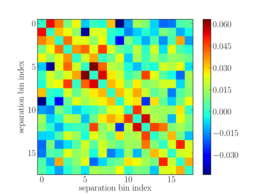
To this end we combined bootstrap matrices from 15 realizations of the mock datasets, i.e. from the full plates. These now hold enough information to create a fully positive-definite covariance matrix by bootstrap. We then inspect the correlation elements in this matrix that span different separations. These elements are small, typically less than . We plot the cross-correlation matrix in the angular separation direction for a fixed choice of and separation bins in Figure 8. While the eye can discern some coherent structures, they do not dominate the matrix.
To make this statement more precise we turn to fitting the bias parameters. We fit for parameters with their redshift evolution with the full bootstrapped covariance matrix and the one in which we have set the non-diagonal elements at different separations to zero. The fitted parameters were unchanged, and the best fit changes by less than 10 units for combined 15 realizations, implying a change of less than unity in per realization. We therefore conclude that for the present analysis, it is a good approximation to assume correlation function measurement errors to be uncorrelated across angular separations.
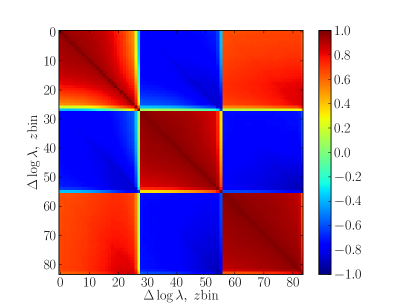
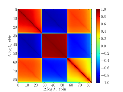
Next we focus on the correlations inside a single angular separation bin. The quadratic estimator covariance matrix has two large eigenvalues corresponding to marginalization over amplitude and spectral slope that were performed as described in Section 3.3 and Appendix B. The bootstrapped covariance matrix of course does not know about this marginalisation, so we manually remove these from the quadratic estimator covariance matrix. This is done by diagonalizing the matrix and then reconstructing it with the two largest eigenvalues set to zero. The resulting correlation matrices are displayed in Figure 9. This result shows that the basic structure of the correlation matrix is correct. However, it is difficult to judge these matrices in detail from the plots and therefore we turn to another test.
3.5.3 The SK test
We measure the correlation function in terms of plates. The quadratic estimator provides a covariance matrix estimate for each individual plate. These are then combined into the complete estimate using
| (3.5) | |||||
| (3.6) |
where the subscript “” denotes the total estimate and the subscript the contribution arising from plate (note that does not denote the vector element). One could make an approximation that within errors of a single plate, the survey mean is a good approximation for the true mean. However, the resulting would be lower than expected, because any given plate has contributed to the total mean. However, it can be shown that the following pseudo [36]
| (3.7) |
has the expected mean for the given number of degrees of freedom. Additionally, if the distribution of the ’s is Gaussian then these quantities are also distributed.
We have performed this test on three sets of data: i) on the reduction where the continuum and other nuisance quantities were assumed to be known perfectly, ii) on the fully analyzed synthetic data and iii) on the data. Results of these tests are presented in Figure 10.
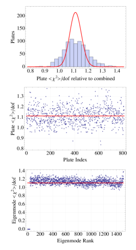
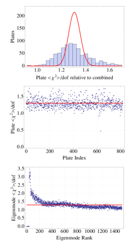
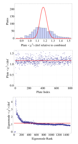
From these plots we can make the following conclusions. First, even when all nuisance quantities are known, the estimator covariance matrix is not perfect as it underestimates the variance by about 10%. This can be due to several reasons, such as the 1D power spectrum not being well estimated, but most likely arises from the fact that the field itself is non-Gaussian. However, the mis-estimate does not seem to correlate with separation, redshift or the magnitude of the eigenvalue contributing to it. When we move our attention to a more realistic analysis in which we fit for the continuum, etc, we find that the estimators make an overall underestimate of the variance by about 35%, but also that this underestimate is primarily produced by the large eigenvalues of . In other words, the noisier eigen-modes of the covariance matrix are more underestimated than the less noisy ones. We find no structure if we slice the data in other parameters (separation, redshift, etc.)
This finding suggests an alternative way of correcting the covariance matrix. We fit the ratio of measured to expected scatter in Figure 10 as a function of eigenvalue rank with a smooth curve and apply it to each covariance matrix separately. The so-constructed matrix will have desired properties in terms of the SK test by construction.
3.5.4 Choice of covariance matrix
To recap this section, we have found that the estimator-provided covariance matrix is a decent approximation, but not sufficiently accurate to provide reliable error-bars. Hence we used three different methods for estimating the errors on our BAO parameters:
-
•
Method 1. Perform the eigen-value decomposition of the estimator matrix into eigenvectors and eigenvalues , and for each eigen-vector we determined the variance predicted by bootstrapped covariance matrix:
(3.8) We set the variance to the larger of the two: and reconstruct the covariance matrix.
-
•
Method 2. Use the eigenvalue-ranked fixed individual matrices as described in Section 3.5.3
-
•
Method 3. Use the bootstrap technique on the final BAO parameters. Generate boot-strap samples as described in Section 3.5.1, then proceed to fit the BAO parameters with it. Use the final distribution of these parameters as an estimate of the uncertainty in those parameters.
As we will see, these estimates provide compatible results in the vicinity of high-likelihood regions. They do, however, differ in the tails of distributions; we will return to this point later.
It might be argued that one should take the version of Method 1 in which the roles of bootstrap and estimator covariance matrices are reverse, i.e. bootstrap matrix is expanded eigenvalue-by-eigenvalue and small eigenvalues corrected by their variances in the estimator matrix. The problem with this approach is that in general eigen-vectors of the bootstrapped matrix are not orthogonal to the 36 large-eigenvalue eigen-vectors in the estimator matrix. We attempted various ways to address this issue, but none produced a satisfactory matrix (i.e. one that would pass tests described in Section 4). We are therefore omitting this approach in the paper.
4 Fitting Baryonic Acoustic Oscillations parameters
The process of fitting the BAO oscillation parameters is described in detail in the companion paper [36]. In short, we model the data as
| (4.1) |
That is, using the standard cosmological model, we convert the observed coordinates (, , ; difference in logarithm of observed wavelength, separation and redshift) into cosmological coordinates () (radial distance in correlation function, angle with respect to the radial direction and redshift). Functions and are multiplicative and additive broadband model discussed below. Our model for is given by
| (4.2) |
where we have decomposed the linear theory correlation function into a smooth component and the peak, but as opposed to most other BAO work, we only dilate the peak part of the correlation function. As discussed in [36], this is the most conservative way of ensuring no information is received from the broadband shape of the correlation function. The cosmological model has an adjustable “peak amplitude” parameter . This amplitude is usually set to unity (recovering the full model), unless we explicitly state that we are fitting for it.
The two isotropic dilation parameters measure the ratio of the BAO standard ruler size, namely sound speed , to the appropriate distance scale
| (4.3) | |||||
| (4.4) |
with respect to our fiducial model, which is flat CDM with , and . In the above equations is the Hubble parameter and is the comoving angular diameter distance.
For most of the test, we perform fits with the isotropic dilation factor which corresponds to the fits where we set (). These isotropic fits fit a single parameter and hence have higher signal-to-noise and are similar to fits to the monopole of the correlation function often performed in the case of galaxy BAO. The reason why our measurement cannot be usefully compressed to quantity lies in the fact that the redshift-space distortion parameter is considerably larger in the case of Lyman- forest, considerably increasing the signal-to-noise ratio in the radial direction. One cannot therefore assume that the relative amount of information coming from and will simply follow the geometrical factors of and respectively.
When fitting the synthetic data we use a linear model, because this is what the synthetic data assumed. However, when fitting the real data, we use the model that has been smoothed to model the weakly non-linear dark matter power spectrum at the redshift of interest. Strictly speaking, this approach is not necessary as it negligibly affects our and only marginally increases our error-bars, as we discuss further in section 5.2.1. We assume that the interpolation in the estimate of the correlation function takes care of the finite bin-size in the correlation function measurement. The linear cosmological model at a given redshift has two parameters: the bias and the redshift-space distortion parameter . Following [34], we use the independent parameters and .
We also use a parameter that governs the redshift evolution of the clustering amplitude, , where is the growth factor. This means that we never explicitly use the growth-factor: we calculate the linear prediction at the reference redshift and then scale the linear power spectrum (together with non-linear corrections) using . Because the inclusion of broadband parameters significantly degrades our ability to measure these parameters we institute a broad Gaussian prior on and .
We additionally fit for a multiplicative broadband () and an additive one (). These two broadband functions are smooth and are designed to remove any non-peak BAO information as described [36]. They are defined to be of the form
| (4.5) |
where is the Legendre polynomial of the -th order and where we fit around 10 parameters simultaneously. In Table 1 we tabulate which combinations of terms we float in the 6 broadband models considered in this paper. We have also investigated less physically motivated broadband models such as those with odd powers of and stronger angular dependencies. All models gave consistent results. For more information see the companion paper [36].
| Name | Type | # free parameters | |||
|---|---|---|---|---|---|
| BB1 | Additive | 0…2 | 0,2,4 | 0 | 9 |
| BB2 | Additive | -2…0 | 0,2,4 | 0 | 9 |
| BB3 | Additive | 0…2 | 0,2 | 0,1 | 12 |
| BB4 | Multiplicative | 0…2 | 0,2,4 | 0 | 8 |
| BB5 | Multiplicative | 0…2 | 0,2 | 0,1 | 10 |
| BB6 | Additive + Multiplicative | 0,1 | 0,2,4 | 0 | 11 |
Our fit uses data in the range . This choice contains sufficiently large buffers at both ends of the fitting range to be able to determine the broadband parameters while preventing the sharp upturn in the correlation function at smaller separations from affecting our fit. We also always cut the data at as these data are the most affected by the sky subtraction residuals [34].
For each model, we minimize , varying all parameters except the parameter of interest, e.g., or /, and then gridding the minimum over the parameters of interest. This procedure is equivalent to marginalizing over all the other parameters in the limit of those marginal likelihoods being Gaussian. This approach is a good approximation when the broadband parameters are not completely degenerate. We have found that combining all broadband models into general broadband models (with parameters) results in the constraints that are very degenerate (in the sense that the data cannot distinguish between terms in the broadband model). In such case, our explicit Monte Carlo tests have shown that the prior volume completely dominates the posterior, or equivalently, the distribution in minimization becomes very non distributed (in the sense that incorrect solutions can be found that are up to away from the true solution).
We calculate uncertainty on the parameters using a Bayesian approach: we convert values into probabilities and then measure the median and relevant points in the cumulative probability distribution. This is an important point as the distribution is non-Gaussian with the confidence limits being asymmetric at a 10% level for our data.
4.1 Tests on synthetic data.
We start by discussing the goodness of fit for our basic fit. These results are shown in Table 2. This table shows that the 15 synthetic mocks on average produce a good that is independent of the broadband model used. We show results for both Method 1 and Method 2 covariance matrices. Table 2 also presents the results of combining fits to the isotropic BAO from all mock realizations; results are consistent with no bias in the method and are consistent between the two methods for estimating the covariance matrix. There is weak evidence that Method 2 might be performing slightly better than Method 1.
| Broadband | BB1 | BB2 | BB3 | BB4 | BB5 | BB6 |
|---|---|---|---|---|---|---|
| Best fit Me1 | ||||||
| Best fit Me2 | ||||||
| Comb. r. Me1 | ||||||
| Comb. r. Me2 |
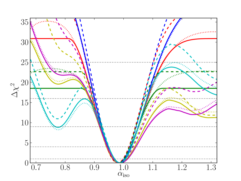
Figure 11 displays the contours for different broadbands for our synthetic data for the isotropic fit for the Method 1 covariance matrix. We also show the results of the combined fit, which was calculated by summing contributions from each individual measurement. The curves are parabolic in the vicinity of the best fit position, but far from this point, they yield a constant for the additive broadband. In those cases, the inferred bias is always close to zero: the model decides that the penalty for having a peak at the wrong position is too large and instead replaces most of the correlations with the broadband model which then makes the fit independent of . This is not the case for broadbands with a multiplicative component, and in this case we indeed see structure outside the most likely region. We also find that for some “lucky” realizations, all broadbands agree on the position of the peak and have the same error-bars, while for some the differences can be staggering. In particular, multiplicative broadbands often latch onto noise features.
The ability of the broadband model to completely replace the true cosmological model when fitting the peak at an undesirable position is unphysical. In other words, one should be able to use the information that there is no evidence for a peak at certain dilations, not just the evidence that there is a peak at others. We can cure this problem by instituting a weak prior on . This prior essentially states that at two sigma, at least one third of the total signal must be cosmological in origin. Note that while the central value of this prior is the same as the value measured in [34], the error is ten times larger, i.e. this is a really weak prior compared to what measurements say about this quantity. curves for those fits are plotted as dotted lines in the Figure 11. The bottom line is that outside the favored region, the difference increases further, but in the region of high-likelihood it is not affected, so this prior will not be used for the final results.
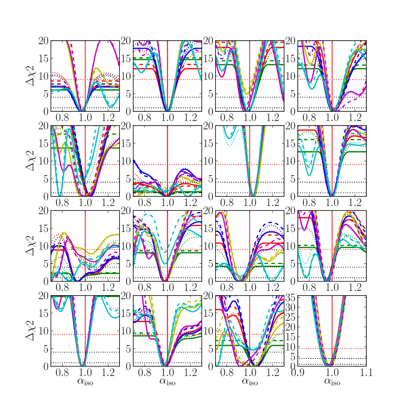
Results for Method 2 are quite similar to those of Method 1. In Figure 11 we also plot comparisons between methods for two ways of estimating covariance method (dashed vs solid lines). We see that Method 2 in general gives higher significance, but not uniformly so.
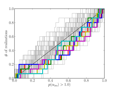
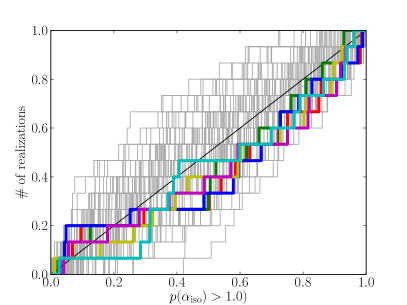
Next we investigate the probability that on each individual mock. If our estimates are unbiased and errors correctly estimated, this probability should be uniformly distributed between and . We plot the cumulative distribution of this quantity in Figure 12.
This figure deserves some attention. From the figure it appears that there might be a mild tension with the expected cumulative distribution. The minimum and maximum values of are around 2-3% and 93-99%, which are consistent with no bias. Plotting the distribution with or produces outliers in the 1 percentile range. Our synthetic datasets share the same continuum realizations and are thus not completely independent, with continuum errors not canceling out when one sums realizations. This results in any one realization being consistent with the correct solution (i.e., no outliers), but they are somewhat correlated leading to skewed plots in Figure 12.
In the absence of a larger number of and more independent synthetic datasets, we associate a % systematic uncertainty with our BAO peak position fitting.
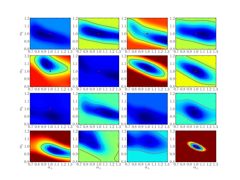
Next we move to the anisotropic fit and relax the assumption of . This is not a purely statistical exercise as the two quantities probe different underlying physical parameters: is a measure of the comoving angular diameter distance to the effective redshift, while is the measure of the local expansion rate at the redshift of interest. If one wants to use our results to estimate cosmological parameters, it is important to distinguish between the two parameters.
We begin by plotting the equivalent of Figure 11 for the anisotropic fit. This is presented in Figure 13. We show plots for one broadband (BB3) and the method 2 covariance matrix. Plots for the method 1 covariance matrix look very similar with larger error-bars. Plots for other broadband models again are similar, although the contours do move for realizations where BAO is only weakly detected. For the strong detections and for the combined fit, the contours are essentially the same.
4.2 Determination of uncertainties
It is clear that for realizations for which the detection of BAO is strong, the likelihood is Gaussian and the error-bars symmetric and Gaussian. In this work we calculate error-bars by applying a uniform prior of between 0.8 and 1.2 and calculating the confidence limits from the appropriate points in the cumulative distribution function. We compare these results with errors derived from a Gaussian expansion of the likelihood around the maximum-likelihood point in Table 3. The -sigma error-bars are always adequately determined by the Gaussian approximation (although also systematically underestimated at a percent level). However, for -sigma error-bars, the Gaussian approximation can fail catastrophically (i.e. the 3-sigma error-bars are limited by the prior). This result is to be expected; when the significance of the BAO detection is low, the information becomes prior dominated at higher levels of confidence [52].
| Set | + | symmetrized | Gaussian approx | |
|---|---|---|---|---|
| Re 7, N=1 | 1.59 | 1.58 | 1.58 | 1.53 |
| Re 7, N=2 | 3.28 | 3.22 | 3.25 | 3.06 |
| Re 7, N=3 | 5.22 | 5.07 | 5.15 | 4.59 |
| Re 8, N=1 | 2.31 | 2.27 | 2.29 | 2.19 |
| Re 8, N=2 | 5.24 | 4.94 | 5.09 | 4.39 |
| Re 8, N=3 | 16 | 15.7 | 15.9 | 6.58 |
| Re 12, N=1 | 2.79 | 2.59 | 2.69 | 2.45 |
| Re 12, N=2 | 8.57 | 5.88 | 7.22 | 4.9 |
| Re 12, N=3 | 23.7 | 14.2 | 18.9 | 7.35 |
| Re 13, N=1 | 1.81 | 1.76 | 1.78 | 1.74 |
| Re 13, N=2 | 3.83 | 3.59 | 3.71 | 3.48 |
| Re 13, N=3 | 6.43 | 5.79 | 6.11 | 5.22 |
5 Results on Baryonic Acoustic Oscillation parameters
We start with the goodness of fit for our data. Fixing BAO parameters to the fiducial cosmological model and using no broadband, we can attempt to fit for the basic bias parameters. With the method 1 covariance matrix we find , and and with 941-3 degrees of freedom. With the method 2 covariance matrix we find , and and . The simplest model of Lyman- forest flux fluctuations, namely that we are measuring a linearly biased tracer of the underlying dark-matter field with Kaiser-like redshift-space distortions, is thus a satisfactory fit with just three floating parameters and is consistent with [34] even when a completely different radial scale range is employed ( in [34] and in this work; lack of small scales is also the reason for increased error-bars in this work despite quadrupling of the number of quasars). Since we have not tested these measurements on synthetic data, we mention them here just to demonstrate that the values are not wildly incompatible with previous measurements.
Table 4 is the equivalent of Table 2 for the data. All broadband models lead to an improvement in compared to the pure cosmology fit, beyond what is expected from extra degrees of freedom. This was not the case in the synthetic data. The values are low but not pathologically so compared to expectation.
| Broadband | BB1 | BB2 | BB3 | BB4 | BB5 | BB6 |
|---|---|---|---|---|---|---|
| Me1 | 855.3 | 857.3 | 830.7 | 864.2 | 849.6 | 856.9 |
| Me2 | 897.5 | 900.2 | 863.7 | 908.4 | 890.5 | 900.1 |
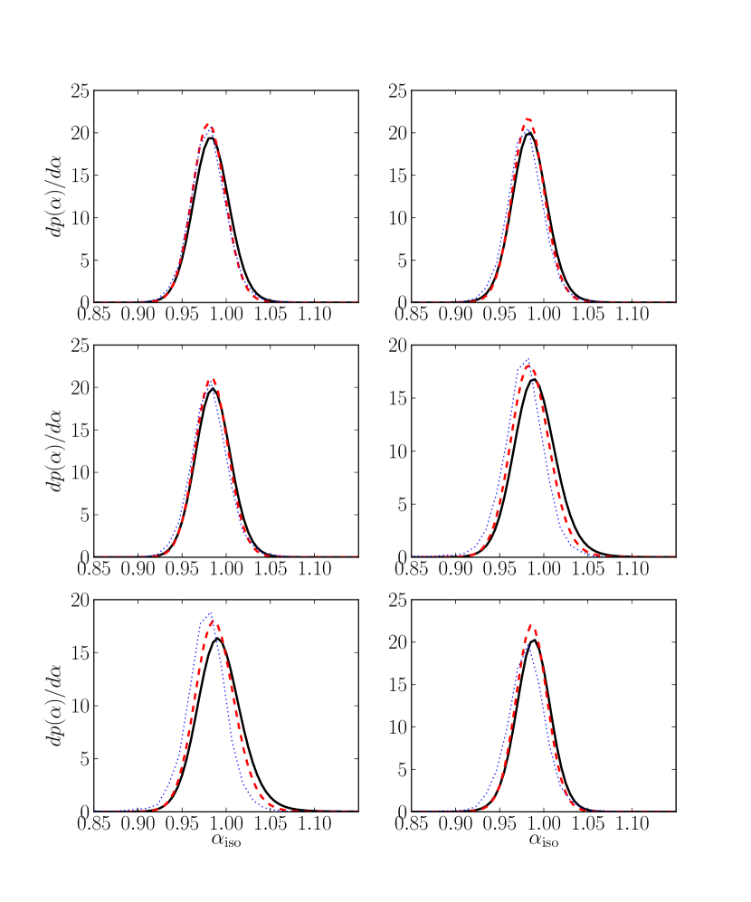
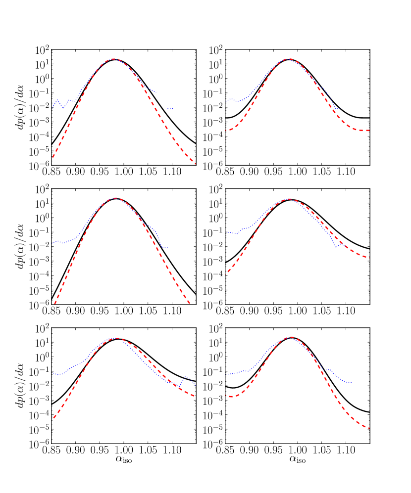
In Figure 14 we show the curves for the data. Even without the prior on bias (dotted lines), we have a solid 4-sigma detection even in the case of the most conservative BB3 prior. The same figure also displays how these constraints depend on the choice of covariance matrix (solid vs dashed lines). Perhaps more relevant are the probability plots, which are shown in Figures 15 and 16. Here we have converted the same values shown before into probabilities and have also added the third method described in Section 3.5.4: bootstrapping on the final parameters. This test treats the bootstrap samples of the BAO parameters as if they were the MCMC samples, i.e., we inferred the probability by treating the number density of the samples as relative probability. Whether this is a statistically sound procedure is not clear as it mixes frequentist and Bayesian statistical approaches. Figure 15 demonstrates excellent agreement between the three methods for most broadband models, except for broadband model 5. The agreement likely stems from the fact that all statistical methods agree in the Gaussian limit. However, when we make the vertical axis logarithmic as we do in Figure 16, we see that bootstrap samples have considerably more outliers than predicted by the Bayesian method. Perhaps the correct conclusion is that our error-bar estimates are sound only to some 3- distance from the most likely point.
| Broadband | BB1 | BB2 | BB3 | BB4 | BB5 | BB6 |
|---|---|---|---|---|---|---|
| Me1 | ||||||
| Me1 w | ||||||
| Me1 w prior | ||||||
| Me1 packed obs. | X | X | X | X | X | X |
| Me1 w Lin. th. | ||||||
| Me1 w alt. NL | ||||||
| Me2 | ||||||
| Me2 w prior | ||||||
| Bootstrap | X | X | X | X | X | X |
| Bootstrap w prior | X | X | X | X | X | X |
These results are numerically condensed in Table 5. The bottom line is that the fit is quite stable with respect to the choice of covariance matrix and the broadband model. Results vary mostly by around and in a few cases by sigma. This result implies that choice of broadband model and covariance matrix are not crucial and that our dominant uncertainty is statistical rather than systematic.
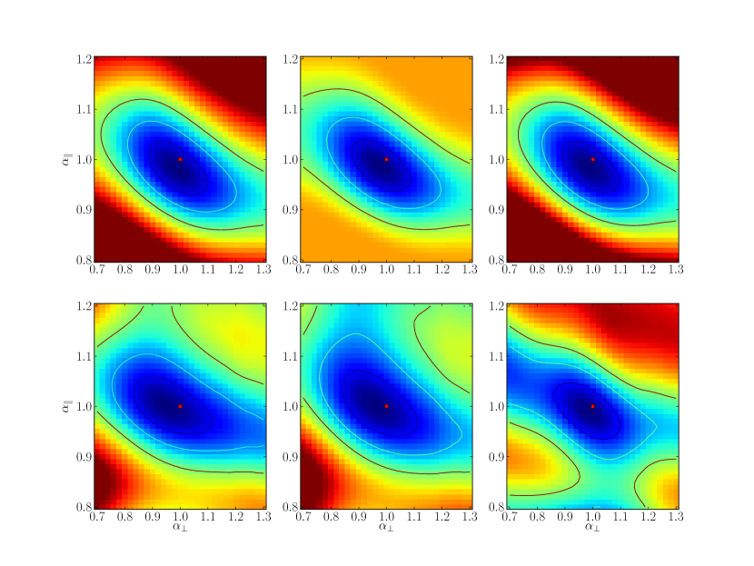
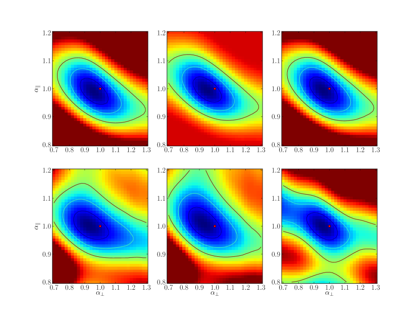
Next we turn to the anisotropic fit. The resulting contours for different broadband models are plotted in Figures 17 and 18. The data are consistent with our fiducial model and stable with respect to the broadband model used for up to two-sigma confidence limits. Beyond that limit, the choice of broadband significantly affects where the contours close. Therefore, given the current signal-to-noise ratio, it is impossible to give a broadband independent statement for allowed range for confidence limits above 95%. We also see that constraints stemming from the method 2 covariance matrix are essentially the same in the shape, but tighter.
5.1 Redshift dependence of BAO position and determination of
We measure the correlation function in three redshift bins at , and . The estimator interpolates between these redshift bins and hence the redshift evolution information is not lost. In order to make cosmological inferences from our dataset, it is important to determine what is the effective redshift at which we measure the position of the BAO.
To find the effect redshift, we add a parameter to our fit that governs the evolution of the BAO scale with redshift: . In other words, we assume that the isotropic scale factor varies as
| (5.1) |
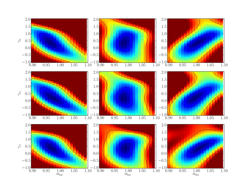
One can expect that measurements of and are correlated so that is best constrained at the position where data are the most constraining. We illustrate this property in Figure 19, where we present the two-dimensional constraints on the - plane for three different choices of . We see the expected behavior as the contours turn their direction as we move from a low reference redshift to a high reference redshift. However, contours are not completely Gaussian; this is expected, when the detection in any one redshift is not very strong. This feature also means that the precise effective redshift is a poorly defined quantity. Different broadbands produce tightest constraints on between and . Therefore we set our . This should not matter for any realistic model that we might want to test using our data. If a cosmological model has a widely varying across small redshift range, then our approach of wide redshift bins fails. In such cases one would expect the peak to be smeared, but, as discussed in the following section, we do not detect any evidence for such effect.
Finally, this figure also demonstrates that the parameter governing the redshift evolution of the BAO peak is consistent with zero, which is by itself a useful systematics check.
5.2 Discussion of systematic effects
The Lyman- forest correlation is a difficult field: systematic effects that affect the measurements of two-point functions are many and closely spaced. However, the BAO measurement is particularly robust. Once the existence of the peak is established in the data, there are few possible systematic effects that can affect its position. Perhaps a suitable analogy is measuring the redshift of a distant object: it is very difficult to spectro-photometrically calibrate spectra even for a well designed modern telescope, but if line features are available in the target spectra, one can nevertheless measure the object’s redshift with considerable precision.
5.2.1 Non-linear effects on the correlation function.
The dark matter field at the redshift relevant for our analysis () is already weakly non-linear, although the effect is considerably smaller than that due to non-linearities (and scale dependent biasing) for galaxy surveys at considerably smaller redshifts. In particular, one expects smoothing of the correlation function in the radial direction and smoothing in the transverse direction [36].
We implemented this smoothing in an approximate manner as described in [36]. In general, the anisotropic smoothing generates multipoles beyond hexadecapole, that depends on both the smoothing parameters and the redshift-space distortion parameters. However, when the smoothing can be treated perturbatively, these multipoles can be ignored and the analysis restricted to multipoles.
Following [8], we only smooth over the peak part of the correlation function, but we have shown explicitly that smoothing the entire linear correlation function affects negligibly. This is expected since we are using only distances .
To further explore this effect, we have also tried a simple isotropic smoothing with kernel size of , and . The error-bars and best-fit in Table 6. Based on , we cannot distinguish the models. We also see that using a smoothed model increases the position error-bars at 10% level and changes the best-fit peak position by a small fraction of standard deviation. Both effects are negligible, but we use the non-linear model for consistency.
Finally, we note that using a model which is unphysically smooth (the isotropic smoothing) decreases the goodness of fit by units. Systematics in the data and processing would typically smooth the peak rather than sharpen it, suggesting that our interpolation scheme is sufficient and that the measured peak has the expected width. The sharpness of the measured peak also precludes fast variations of the peak position with redshift, which would result in further smoothing of the BAO peak.
| Model | Best Fit | |
|---|---|---|
| linear | 831 | |
| non-linear | 830.698 | |
| Alt. non-linear | 830.73 | |
| 3 iso. smooth | 830.775 | |
| 6 iso. smooth | 831.29 | |
| 12 , iso. smooth | 838.446 |
5.2.2 Data cuts
We explicitly investigated a few possible systematic effects, by restricting the analysis to a subset of data and rerunning our correlation function analysis to see if the peak position is affected more than one would anticipate given the amount of the data removed. In particular, we have performed the following tests:
-
•
Removing the data at the ultraviolet end of the spectrograph. We normally use the data redward of Å. The spectra at the ultraviolet end of the wavelength range are the least understood part of the data. They are difficult to calibrate spectro-photometrically due to nature of the calibration stars. This is exacerbated by the fact that quasar fibers were drilled in a plate position which, given atmospheric dispersion, maximizes the blue throughput relevant for the Lyman- forest rather than the red throughput used for other objects and calibration stars. Hence for this test we remove the data between Åand Å.
-
•
Spectro-photometric variability. This cut is another way of examining the effect of poor spectro-photometry at the blue-end of the spectrograph. For every quasar, we calculate two variability scores (“slope” and “normalization”) as follows. For each individual exposure, the mean inverse variance weighted flux is calculated in two wavelength bands (4000-4500 Åand 5500-6000 Å). The “slope” (“normalization”) score is calculated using a weighted average of the deviations of the differences (sums) of the mean flux in the two bands for an individual exposure to the mean from the differences (sums) of the mean flux in the two bands for all the exposures corresponding to a single observation. We then remove 10% of the quasars that show the most exposure-to-exposure variability in the sum of “slope” and “normalization” variability scores.
-
•
A more conservative upper rest-frame cut. In our standard analysis, we use an aggressive upper rest-frame cut of Å, going nearly up to the actual Lyman- emission line. We check the results by restricting to a much more conservative Å
-
•
DLA cut. Normally, we use quasars that have an identified DLA system, but we exclude the data from 1.5 equivalent widths around the DLA. In this test we have removed all quasars that contained one or more DLA systems.
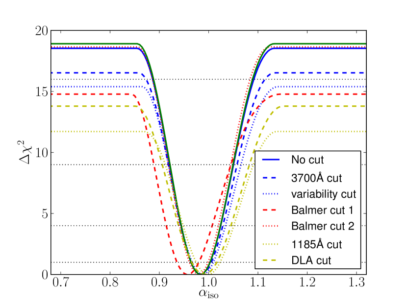
Figure 20: Results of the systematics test. The blue solid line is our default data reduction. We additionally plot results from the Åcut (blue dotted), variability cut (blue dashed), DLA cut (yellow dashed), cut (yellow dotted) and Balmer line cuts (red dotted and dashed). Solid green line shows result upon addition of parameter. All tests are done for the entire data for broadband model BB2 with method 1 covariance matrix. Other fits shows similar change. See text for discussion. -
•
Balmer line cuts. We investigated the effect of cutting around the position of the observed frame Balmer lines. As discussed in the Section 3.1, we see features due to mis-calibration. If these mis-calibration features were correlated, these could produce correlated systematic signal at fixed radial distances. In order to check for the effect, we have reanalyzed our data with two separate cuts eliminating data in Åand Å.
The results of these tests are shown in Figure 20. None of the cuts affect the data significantly except potentially the ÅBalmer line cut. This effect has been analyzed in [35] and we show explicitly that data are statistically consistent with the full sample in Appendix D.
The same figure also shows the effect of adding a parameter describing the redshift evolution of redshift-space parameter , namely ; this result also appears in the Table 5. This parameter has negligible effect, regardless of the broadband being employed.
5.2.3 Other systematics
There are additional potential sources of systematics which we argue are negligible in this work:
-
•
Metal contamination. Another important systematic effect might be metal contamination [53]. The strongest is Si III, which absorbs at Å, producing a correlated absorption separated by 2271 km/s from the Lyman- absorption by the same gas, corresponding to around of radial separation. The largest contribution is the Lyman- -Si III contamination, which is suppressed by a factor of with respect to the Lyman- – Lyman- correlation. In other words, the measured correlation function in the fiducial cosmology is the true cosmology plus a suppressed shadow with radial distances shifted by . We thus expect the contribution from Si III to be negligible unless our amplitude accuracy begins to approach of the total peak height. This warrants further investigation along with the impact of weaker metal lines and we will do so in a future publication.
-
•
Binning artifacts. In principle, when one uses flat bins to estimate the correlation function, it is possible that the actual bin centers do not correspond to the true bin centers, thus skewing the measurement of the BAO position. For example, if the number of pairs is a steeply falling/increasing function of separation, then the actual mean separation of pairs contributing to a given bin of correlation function will be less/more than the nominal bin center. This is alleviated by linearly interpolating between any two bins in radial and redshift directions (instead of using top hat bins). We have also tested our procedures on synthetic datasets with exactly the same geometry as the real dataset.
-
•
Wavelength and astrometric calibration. Radially, the BAO distance corresponds to a separation in wavelength. The relative wavelength calibration is better than [32] and therefore well under the required precision. Transverse, the BAO distance corresponds to an angular separation of the order . The angular separation between any two quasars is known to arc-second precision and in addition these errors are not coherent. This is another completely negligible effect.
5.3 Consensus result
We have presented a number of results which are reasonably consistent, but vary in precise values, because of different assumed covariance matrix and broadband model. However, it is useful to reduce this variety to a single consensus value.
We show the marginalized confidence limits for all broadband models and both covariance matrices in Table 7. These limits were derived from the cumulative distribution functions of marginalized likelihoods as described in the Section 4.2. The marginalized error-bars on the and are significantly larger than the errors on the isotropic fit. This degeneracy is due to large cross-correlation coefficient between the two parameters, which is estimated to be by fitting a Gaussian to the best-fit model.
| Model | |||
|---|---|---|---|
| BB1 Me1 | |||
| BB1 Me2 | |||
| BB2 Me1 | |||
| BB2 Me2 | |||
| BB3 Me1 | |||
| BB3 Me2 | |||
| BB4 Me1 | |||
| BB4 Me2 | |||
| BB5 Me1 | |||
| BB5 Me2 | |||
| BB6 Me1 | |||
| BB6 Me2 |
For the final results, we would like to quote a consensus result that captures the statistical and systematic uncertainty. To this end we select the broadband 2 model with the less constraining (method 1) covariance matrix. Inspecting the table 7 we see that it has values and errors that are not at the edges of distributions. Figure 14 shows that it is the most conservative of the additive broadbands. We could use the most relaxing broadband 6, however, this model latches onto a noise feature at , which breaks its 3-sigma errors assuming the noise feature is indeed not real (no other broadband can fit it and it becomes weaker with the more constraining method 2 covariance matrix). Therefore we absorb these uncertainties by specifying systematic errors that should contain them. Hence we quote our fit
| (stat.) (syst.) | (5.2) |
for the isotropic fit and
| (stat.) (syst.) | (5.3) | ||
| (stat.) (syst.) | (5.4) |
for the anisotropic fit. We are not quoting the marginalized 3-sigma error in the , as it is dominated by the top-hat prior on the - plane. Note, however, that this is not true for the un-marginalized likelihood, as large parts of the - plane are excluded by our measurement, even for the less constraining models.
The systematic error should be understood as having a top-hat probability distribution function, and thus while significantly affecting the 1-sigma confidence limits, its effect on the 3-sigma confidence limits are considerably smaller.
The fact that our quoted systematic errors are of the same order as one-sigma statistical errors is not coincidental. As the signal-to-noise ratio will improve with additional data, so will our ability to constrain the broadband model, and the differences between best-fit values for different broadband models will naturally decrease.
5.4 Comparison to Busca et al.
In [35] we presented an analysis of the BAO in the Lyman- forest from a very similar dataset. The two analyses are complementary and the present analysis builds upon the previous work. The main methodological differences between the two can be summarized as follows:
-
•
The analysis in [35] uses more conservative cuts in their choice of data. They exclude all quasars in which one or more DLAs are present as indicated by the visual inspection, while we remove only 1.5 equivalent widths around the position of the DLA. We also use a slightly different DLA catalog from [43]. Moreover, we aggressively use as much of the forest as available (Å-Å rest-frame for non-BAL quasars), while [35] restrict the analysis to Å-Å rest-frame. These different restrictions are responsible for most of the increase in the signal-to-noise in the present paper.
-
•
The continuum fitting procedure is different in the two analyses.
-
•
We use considerably finer binning in our correlation function. In particular we measure the correlation function in three redshift bins and for each redshift bin we measure it in 18 transverse and 28 radial bins. The analysis in [35] uses 2D measurement as an intermediate measurement, but they eventually compress all data into 90 measurements of the monopole and quadrupole of the correlation function for a given fiducial cosmology. The finer binning has an advantage that it is in principle easier to catch systematic errors that are localized in particular bins of the measured correlation function; however, the larger number of bins makes measuring and understanding of the covariance matrix considerably more difficult.
-
•
The analysis in [35] uses diagonal weighting with a fixed assumption about the amplitude evolution of the forest correlations with redshift, but allow for a completely unconstrained parameter (we institute a weak prior on to regularize fits)
-
•
The analysis in [35] makes stronger assumptions about the broadband and in particular do not consider a multiplicative broadband.
-
•
The analysis in [35] uses a wider fitting range vs employed in this paper.
-
•
The analysis in [35] does not take into account the broadening of the peak by non-linear evolution. We show that this has a negligible effect on the position and only small effect on the errors.
In [35] the isotropic dilation factors has been determined to be , to be compared with our result (stat.) (syst.). This is a one sigma difference, from what might appear to be essentially the same dataset. We use looser cuts on data, but our detection significance has improved more than one would expect based on the increase in the number of data-points alone. The same has been observed, when more inclusive cuts have been applied to the [35] analysis (N. Busca, private communication), so this result seems to be a feature of the sample. Given the increase in the signal-to-noise ratio, the difference is not statistically significant.
5.5 Consistency with SPT and BOSS galaxy BAO results
Recently, the measurements of the acoustic oscillations in the Cosmic Microwave Background by the SPT experiment [54], combined with WMAP7 results [55] predicted a position for the BAO peak at in the simplest flat CDM model, which is in tension with the measurements of the BAO in the CMASS galaxies from the BOSS experiment [8]. We briefly discuss this tension in the context of our measurement.
We show results for the quantities of interest for several standard models in Table 8. In the cosmology of the CMASS fiducial model, the SPT result can be cast as a measurement of , while the “consensus value” (after reconstruction) for the CMASS measurement is . The difference is discrepant at 2.3-sigma assuming the errors can be added in quadrature. We will not discuss the details of this discrepancy (see e.g. [56]), but instead ask if Lyman- forest BAO can add anything to this discussion. To this end we added two modification of the CMASS fiducial model to Table 8 that have the same value of as the CMASS best fit, either by changing the value of or .
Inspecting Table 8 show that the SPT best and CMASS best models predict values of that differ by less than our uncertainties. Differences in are of the order of 0.5%, while changes to are of the order of 2%, both small compared to our error-bars. When correctly taking into account the covariance between and , the size of the effect is larger, but BOSS Lyman- forest BAO is currently unable to distinguish between the models in a statistically significant manner.
Therefore, Lyman- forest BAO will not be able to distinguish between these models in the CDM scenario. This is because the Kaiser redshift-space distortion parameter is large for the Lyman- forest, pushing the statistical weight of the BAO signal towards the measurements of Hubble parameter (where the effect is small) rather than angular diameter distance (where the effect is large). This is an expected result[3]. Lyman- forest BAO measurements do not improve the constraints to the minimal flat CDM model. It does, however, help constrain models with non-zero curvature or dark energy that is dynamically significant at high redshift.
| Model | |||||
|---|---|---|---|---|---|
| Lyman- fid | 0.0227 | 0.1096 | 0.700 | 1.0347 | 146.90 |
| SPT best | 0.0229 | 0.1093 | 0.731 | 1.0396 | 146.83 |
| CMASS fid | 0.0224 | 0.1119 | 0.7 | 1.0382 | 146.51 |
| CMASS best 1 | 0.0224 | 0.1119 | 0.668 | 1.0287 | 146.51 |
| CMASS best 2 | 0.0224 | 0.1192 | 0.673 | 1.0382 | 144.57 |
| Lyman- | BOSS galaxies | |||||
|---|---|---|---|---|---|---|
| Lyman- fid | 35290 | 2.5484 | 1 | 1 | 7.5576 | 1.001 |
| SPT best | 35384 | 2.5975 | 0.997 | 0.981 | 7.7869 | 0.971 |
| CMASS fid | 35464 | 2.5544 | 0.995 | 0.997 | 7.5625 | 1.000 |
| CMASS best 1 | 35326 | 2.5001 | 1.00 | 1.022 | 7.3201 | 1.033 |
| CMASS best 2 | 35738 | 2.5122 | 0.992 | 1.017 | 7.3198 | 1.033 |
6 Visualizing the peak
Errors in the correlation function measurements are always significantly more correlated than the errors in a more natural space for two-point function such as Fourier space measurement. In our case, the marginalization over the unwanted modes makes this issue particularly acute - one obtains unbiased estimates at the price of large, but nearly perfectly correlated uncertainties. We also measure the correlation function in many points, each of which is rather noisy. Moreover, some of the BAO signal is in the monopole while some is in the quadrupole. Nevertheless, one would still wish to simply “see” the BAO peak and produce the peak plots in an objective manner.
To this end we compress the measured correlation function as follows. We fit for a cosmological model with broadband. We then fix the parameters of this model, set the BAO amplitude to zero and fit for the binned deviations of the real space correlation function. The real space correlation function is piece-wise linearly interpolated between bins in the . Given the best-fit value we propagate this fit to the monopole to higher multipoles. The result of this exercise is an optimally estimated real-space correlation function that has Kaiser-like redshift-space distortions. Since we are fitting around the model without the BAO peak, this fit has no way of knowing about the existence or the position of the BAO peak.
However, the resulting correlation function will still have large correlated errors. We can remove these, by diagonalizing the covariance matrix of our fitted binned correlation function and setting the amplitude of the largest eigen-mode to zero. At the same time, we must also project out the same eigen-vector from the theory. We have thus made a full circle; we end up with a distorted correlation function and a theory that accounts for this distortion.
Results of this exercises are plotted in Figure 21 for data and for the mean of all realizations of synthetic data. Removing more than one eigenvalue produces essentially the same plots.
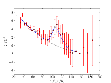 |
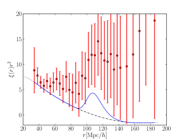 |
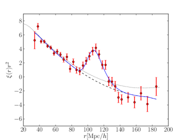 |
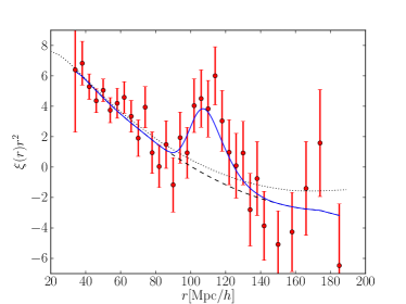 |
7 Discussion & Conclusions
In this paper we have revisited the measurement of the Lyman- forest BAO. We have detected the baryonic acoustic oscillations in the flux fluctuations in the Lyman- forest of distant quasars which allows a measurement of the expansion rate at a redshift of . We have confirmed an earlier result with a significantly different method and data cuts.
Our results are consistent with but more stringent than [35]. By far the most important reason for this improvement is that we use more data by imposing looser cuts (which we think is valid when one tries to find an isolated feature such as BAO peak). Second, we use an optimal estimator, which should increase the available signal-to-noise ratio by 10-20% as indicated by tests on fields with known continuum. Finally, we use a much finer binning, resulting in less information loss when simultaneously fitting for the BAO and broadband parameters.
Our results are more precise than the theoretical expectations for what the BOSS experiment with the present dataset is expected to achieve with the Lyman- forest technique [25]. The covariance of and measurements have the same correlation coefficient as predicted by the Fisher matrix forecast (), but our signal-to-noise is about 40% better. The Fisher matrix calculation assumed bias parameters from [19] and the forecasted expectations for the BOSS spectrograph signal-to-noise. In fact we have now achieved the statistical position accuracy that is consistent with what would be expected at the end of the survey. We saw with the synthetic data that realization-to-realization scatter is large so it is possible that we might just have been fortunate. On the other hand, it is also possible that the forecasts were pessimistic and that the signal is larger than expected. To distinguish between these possibilities, one needs to perform the analysis on a larger dataset and/or carefully compare the achieved spectrograph signal-to-noise and measured bias parameters with values that were used in the Fisher matrix analysis.
We fitted different broadband models and found that these produce shifts in the best-fit values of BAO position of the order of the 1-sigma statistical errors. This effect is similar to the difference between the correlation function analysis and the power spectrum analysis in [8] – there is just one two-point function and hence different results reflect how a broadband model parametrized in Fourier or configuration space is simply a different model leading to different results. As the signal-to-noise increases, the likelihoods will become more Gaussian, which will make it easier to make sense of differing results from different broadband models.
We attempted to be conservative when quoting our results: we used the least constraining broadband model and the less constraining of our two covariance matrices. We also assigned differences between best-fit models from different broadbands to systematic error. Using these criteria, we measure (stat.) (syst.) with respect to the fiducial model (flat CDM with , ) for the isotropic dilation factor and we find marginalized constraints (stat.) (syst.) and (stat.) (syst.) for the anisotropic fit.
We do not attempt to present a precise number for the statistical significance of the peak detection. Assuming our most optimistic broadband model, our significance is well over 5-sigma. Believing that the main solution is the correct one, but choosing our most conservative broadband models reduce it to -sigma. Taking seriously the secondary solution at found by the broadband model 6, the significance drops to -sigma.
To a large extent, the question of the BAO peak significance is a moot point. One is measuring the BAO position in order to learn about possible and impossible cosmological models. Plausible cosmological models will not deviate from concordance by more than a few percent and hence stay in the region where all methods give consistent results on the peak position.
An important lesson learned in this work is that it is essential to have a method that is computationally feasible enough to analyze not just the real dataset, but many (hundreds) of realizations of the mock data to gain full understanding of the estimator and possible systematics effects arising from the analyses. What we might have gained in statistical errors was lost in our ability to fully characterize the estimator using a large number of realizations. However, when going beyond measuring BAO and attempting to use the broadband power to constrain cosmology, an approach similar to the one employed in this work will be necessary to deal with the continuum-fitting induced distortion. In addition, a better analysis requires a more sophisticated continuum fitting and instrument model and will require a red-side systematics subtraction. In short, it is clear that many improvements can be made in the Lyman- forest data reduction methodology.
We defer deriving cosmological constraints from the position of the BAO peak to a future publication. The current measurement of the BAO peak position is a striking confirmation of our basic understanding of the universe, as pointed out in [35]; and we expect it to be very competitive for models with early dark energy and curvature.
Acknowledgments
Funding for SDSS-III has been provided by the Alfred P. Sloan Foundation, the Participating Institutions, the National Science Foundation, and the U.S. Department of Energy Office of Science. The SDSS-III web site is http://www.sdss3.org/.
SDSS-III is managed by the Astrophysical Research Consortium for the Participating Institutions of the SDSS-III Collaboration including the University of Arizona, the Brazilian Participation Group, Brookhaven National Laboratory, University of Cambridge, Carnegie Mellon University, University of Florida, the French Participation Group, the German Participation Group, Harvard University, the Instituto de Astrofisica de Canarias, the Michigan State/Notre Dame/JINA Participation Group, Johns Hopkins University, Lawrence Berkeley National Laboratory, Max Planck Institute for Astrophysics, Max Planck Institute for Extraterrestrial Physics, New Mexico State University, New York University, Ohio State University, Pennsylvania State University, University of Portsmouth, Princeton University, the Spanish Participation Group, University of Tokyo, University of Utah, Vanderbilt University, University of Virginia, University of Washington, and Yale University.
References
- [1] A. G. Riess, A. V. Filippenko, P. Challis, A. Clocchiatti, A. Diercks, P. M. Garnavich, R. L. Gilliland, C. J. Hogan, S. Jha, R. P. Kirshner, B. Leibundgut, M. M. Phillips, D. Reiss, B. P. Schmidt, R. A. Schommer, R. C. Smith, J. Spyromilio, C. Stubbs, N. B. Suntzeff, and J. Tonry, Observational Evidence from Supernovae for an Accelerating Universe and a Cosmological Constant, AJ 116 (Sept., 1998) 1009–1038, [astro-ph/].
- [2] S. Perlmutter, G. Aldering, G. Goldhaber, R. A. Knop, P. Nugent, P. G. Castro, S. Deustua, S. Fabbro, A. Goobar, D. E. Groom, I. M. Hook, A. G. Kim, M. Y. Kim, J. C. Lee, N. J. Nunes, R. Pain, C. R. Pennypacker, R. Quimby, C. Lidman, R. S. Ellis, M. Irwin, R. G. McMahon, P. Ruiz-Lapuente, N. Walton, B. Schaefer, B. J. Boyle, A. V. Filippenko, T. Matheson, A. S. Fruchter, N. Panagia, H. J. M. Newberg, W. J. Couch, and The Supernova Cosmology Project, Measurements of Omega and Lambda from 42 High-Redshift Supernovae, ApJ 517 (June, 1999) 565–586, [astro-ph/].
- [3] D. H. Weinberg, M. J. Mortonson, D. J. Eisenstein, C. Hirata, A. G. Riess, and E. Rozo, Observational Probes of Cosmic Acceleration, ArXiv e-prints (Jan., 2012) [arXiv:1201.2434].
- [4] H.-J. Seo and D. J. Eisenstein, Probing Dark Energy with Baryonic Acoustic Oscillations from Future Large Galaxy Redshift Surveys, ApJ 598 (Dec., 2003) 720–740, [astro-ph/].
- [5] D. J. Eisenstein, I. Zehavi, D. W. Hogg, R. Scoccimarro, M. R. Blanton, R. C. Nichol, R. Scranton, H.-J. Seo, M. Tegmark, Z. Zheng, S. F. Anderson, J. Annis, N. Bahcall, J. Brinkmann, S. Burles, F. J. Castander, A. Connolly, I. Csabai, M. Doi, M. Fukugita, J. A. Frieman, K. Glazebrook, J. E. Gunn, J. S. Hendry, G. Hennessy, Z. Ivezić, S. Kent, G. R. Knapp, H. Lin, Y.-S. Loh, R. H. Lupton, B. Margon, T. A. McKay, A. Meiksin, J. A. Munn, A. Pope, M. W. Richmond, D. Schlegel, D. P. Schneider, K. Shimasaku, C. Stoughton, M. A. Strauss, M. SubbaRao, A. S. Szalay, I. Szapudi, D. L. Tucker, B. Yanny, and D. G. York, Detection of the Baryon Acoustic Peak in the Large-Scale Correlation Function of SDSS Luminous Red Galaxies, ApJ 633 (Nov., 2005) 560–574.
- [6] H.-J. Seo and D. J. Eisenstein, Baryonic Acoustic Oscillations in Simulated Galaxy Redshift Surveys, ApJ 633 (Nov., 2005) 575–588, [astro-ph/].
- [7] N. Padmanabhan, X. Xu, D. J. Eisenstein, R. Scalzo, A. J. Cuesta, K. T. Mehta, and E. Kazin, A 2% Distance to z=0.35 by Reconstructing Baryon Acoustic Oscillations - I : Methods and Application to the Sloan Digital Sky Survey, ArXiv e-prints (Jan., 2012) [arXiv:1202.0090].
- [8] L. Anderson, E. Aubourg, S. Bailey, D. Bizyaev, M. Blanton, A. S. Bolton, J. Brinkmann, J. R. Brownstein, A. Burden, A. J. Cuesta, L. N. A. da Costa, K. S. Dawson, R. de Putter, D. J. Eisenstein, J. E. Gunn, H. Guo, J.-C. Hamilton, P. Harding, S. Ho, K. Honscheid, E. Kazin, D. Kirkby, J.-P. Kneib, A. Labatie, C. Loomis, R. H. Lupton, E. Malanushenko, V. Malanushenko, R. Mandelbaum, M. Manera, C. Maraston, C. K. McBride, K. T. Mehta, O. Mena, F. Montesano, D. Muna, R. C. Nichol, S. E. Nuza, M. D. Olmstead, D. Oravetz, N. Padmanabhan, N. Palanque-Delabrouille, K. Pan, J. Parejko, I. Paris, W. J. Percival, P. Petitjean, F. Prada, B. Reid, N. A. Roe, A. J. Ross, N. P. Ross, L. Samushia, A. G. Sanchez, D. J. S. D. P. Schneider, C. G. Scoccola, H.-J. Seo, E. S. Sheldon, A. Simmons, R. A. Skibba, M. A. Strauss, M. E. C. Swanson, D. Thomas, J. L. Tinker, R. Tojeiro, M. Vargas Magana, L. Verde, C. Wagner, D. A. Wake, B. A. Weaver, D. H. Weinberg, M. White, X. Xu, C. Yeche, I. Zehavi, and G.-B. Zhao, The clustering of galaxies in the SDSS-III Baryon Oscillation Spectroscopic Survey: Baryon Acoustic Oscillations in the Data Release 9 Spectroscopic Galaxy Sample, ArXiv e-prints (Mar., 2012) [arXiv:1203.6594].
- [9] C. Blake, S. Brough, M. Colless, C. Contreras, W. Couch, S. Croom, D. Croton, T. M. Davis, M. J. Drinkwater, K. Forster, D. Gilbank, M. Gladders, K. Glazebrook, B. Jelliffe, R. J. Jurek, I.-h. Li, B. Madore, D. C. Martin, K. Pimbblet, G. B. Poole, M. Pracy, R. Sharp, E. Wisnioski, D. Woods, T. K. Wyder, and H. K. C. Yee, The WiggleZ Dark Energy Survey: joint measurements of the expansion and growth history at z 1, MNRAS 425 (Sept., 2012) 405–414, [arXiv:1204.3674].
- [10] D. Schlegel, F. Abdalla, T. Abraham, C. Ahn, C. Allende Prieto, J. Annis, E. Aubourg, M. Azzaro, S. B. C. Baltay, C. Baugh, C. Bebek, S. Becerril, M. Blanton, A. Bolton, B. Bromley, R. Cahn, P. . Carton, J. L. Cervantes-Cota, Y. Chu, M. Cortes, K. Dawson, A. Dey, M. Dickinson, H. T. Diehl, P. Doel, A. Ealet, J. Edelstein, D. Eppelle, S. Escoffier, A. Evrard, L. Faccioli, C. Frenk, M. Geha, D. Gerdes, P. Gondolo, A. Gonzalez-Arroyo, B. Grossan, T. Heckman, H. Heetderks, S. Ho, K. Honscheid, D. Huterer, O. Ilbert, I. Ivans, P. Jelinsky, Y. Jing, D. Joyce, R. Kennedy, S. Kent, D. Kieda, A. Kim, C. Kim, J. . Kneib, X. Kong, A. Kosowsky, K. Krishnan, O. Lahav, M. Lampton, S. LeBohec, V. Le Brun, M. Levi, C. Li, M. Liang, H. Lim, W. Lin, E. Linder, W. Lorenzon, A. de la Macorra, C. Magneville, R. Malina, C. Marinoni, V. Martinez, S. Majewski, T. Matheson, R. McCloskey, P. McDonald, T. McKay, J. McMahon, B. Menard, J. Miralda-Escude, M. Modjaz, A. Montero-Dorta, I. Morales, N. Mostek, J. Newman, R. Nichol, P. Nugent, K. Olsen, N. Padmanabhan, N. Palanque-Delabrouille, I. Park, J. Peacock, W. Percival, S. Perlmutter, C. Peroux, P. Petitjean, F. Prada, E. Prieto, J. Prochaska, K. Reil, C. Rockosi, N. Roe, E. Rollinde, A. Roodman, N. Ross, G. Rudnick, V. Ruhlmann-Kleider, J. Sanchez, D. Sawyer, C. Schimd, M. Schubnell, R. Scoccimaro, U. Seljak, H. Seo, E. Sheldon, M. Sholl, R. Shulte-Ladbeck, A. Slosar, D. S. Smith, G. Smoot, W. Springer, A. Stril, A. S. Szalay, C. Tao, G. Tarle, E. Taylor, A. Tilquin, J. Tinker, F. Valdes, J. Wang, T. Wang, B. A. Weaver, D. Weinberg, M. White, M. Wood-Vasey, J. Yang, X. Y. C. Yeche, N. Zakamska, A. Zentner, C. Zhai, and P. Zhang, The BigBOSS Experiment, ArXiv e-prints (June, 2011) [arXiv:1106.1706].
- [11] C. L. Reichardt, R. de Putter, O. Zahn, and Z. Hou, New Limits on Early Dark Energy from the South Pole Telescope, ApJL 749 (Apr., 2012) L9, [arXiv:1110.5328].
- [12] U. Alam, Constraining Perturbative Early Dark Energy with Current Observations, ApJ 714 (May, 2010) 1460–1469, [arXiv:1003.1259].
- [13] J.-Q. Xia and M. Viel, Early dark energy at high redshifts: status and perspectives, JCAP 4 (Apr., 2009) 2, [arXiv:0901.0605].
- [14] E. V. Linder and G. Robbers, Shifting the Universe: early dark energy and standard rulers, JCAP 6 (June, 2008) 4, [arXiv:0803.2877].
- [15] M. Doran and G. Robbers, Early dark energy cosmologies, JCAP 6 (June, 2006) 26, [astro-ph/].
- [16] M. Doran, J.-M. Schwindt, and C. Wetterich, Structure formation and the time dependence of quintessence, Phys. Rev. D 64 (Dec., 2001) 123520, [astro-ph/].
- [17] R. Lynds, The Absorption-Line Spectrum of 4c 05.34, ApJL 164 (Mar., 1971) L73+.
- [18] L. Hui and N. Y. Gnedin, Equation of state of the photoionized intergalactic medium, MNRAS 292 (Nov., 1997) 27–+.
- [19] P. McDonald, Toward a Measurement of the Cosmological Geometry at z ~ 2: Predicting Ly Forest Correlation in Three Dimensions and the Potential of Future Data Sets, ApJ 585 (Mar., 2003) 34–51, [astro-ph/].
- [20] N. Kaiser, Clustering in real space and in redshift space, MNRAS 227 (July, 1987) 1–21.
- [21] A. Slosar, S. Ho, M. White, and T. Louis, The acoustic peak in the Lyman alpha forest, JCAP 10 (Oct., 2009) 19–+, [arXiv:0906.2414].
- [22] M. White, A. Pope, J. Carlson, K. Heitmann, S. Habib, P. Fasel, D. Daniel, and Z. Lukic, Particle Mesh Simulations of the Ly Forest and the Signature of Baryon Acoustic Oscillations in the Intergalactic Medium, ApJ 713 (Apr., 2010) 383–393, [arXiv:0911.5341].
- [23] P. McDonald, Toward a Measurement of the Cosmological Geometry at z ~ 2: Predicting Ly Forest Correlation in Three Dimensions and the Potential of Future Data Sets, ApJ 585 (Mar., 2003) 34–51, [astro-ph/].
- [24] M. White, The Ly-a forest, in The Davis Meeting On Cosmic Inflation. 2003 March 22-25, Davis CA., p.18, Mar., 2003.
- [25] P. McDonald and D. J. Eisenstein, Dark energy and curvature from a future baryonic acoustic oscillation survey using the Lyman- forest, Phys. Rev. D 76 (Sept., 2007) 063009–+, [astro-ph/].
- [26] K. S. Dawson, D. J. Schlegel, C. P. Ahn, S. F. Anderson, E. Aubourg, S. Bailey, R. H. Barkhouser, J. E. Bautista, A. Beifiori, A. A. Berlind, V. Bhardwaj, D. Bizyaev, C. H. Blake, M. R. Blanton, M. Blomqvist, A. S. Bolton, A. Borde, J. Bovy, W. N. Brandt, H. Brewington, J. Brinkmann, P. J. Brown, J. R. Brownstein, K. Bundy, N. G. Busca, W. Carithers, A. R. Carnero, M. A. Carr, Y. Chen, J. Comparat, N. Connolly, F. Cope, R. A. C. Croft, A. J. Cuesta, L. N. da Costa, J. R. A. Davenport, T. Delubac, R. de Putter, S. Dhital, A. Ealet, G. L. Ebelke, D. J. Eisenstein, S. Escoffier, X. Fan, N. Filiz Ak, H. Finley, A. Font-Ribera, R. Genova-Santos, J. E. Gunn, H. Guo, D. Haggard, P. B. Hall, J.-C. Hamilton, B. Harris, D. W. Harris, S. Ho, D. W. Hogg, D. Holder, K. Honscheid, J. Huehnerhoff, B. Jordan, W. P. Jordan, G. Kauffmann, E. A. Kazin, D. Kirkby, M. A. Klaene, J.-P. Kneib, J.-M. Le Goff, K.-G. Lee, D. C. Long, C. P. Loomis, B. Lundgren, R. H. Lupton, M. A. G. Maia, M. Makler, E. Malanushenko, V. Malanushenko, R. Mandelbaum, M. Manera, C. Maraston, D. Margala, K. L. Masters, C. K. McBride, P. McDonald, I. D. McGreer, O. Mena, J. Miralda-Escude, A. D. Montero-Dorta, F. Montesano, D. Muna, A. D. Myers, T. Naugle, R. C. Nichol, P. Noterdaeme, M. D. Olmstead, A. Oravetz, D. J. Oravetz, R. Owen, N. Padmanabhan, N. Palanque-Delabrouille, K. Pan, J. K. Parejko, I. Paris, W. J. Percival, I. Perez-Fournon, I. Perez-Rafols, P. Petitjean, R. Pfaffenberger, J. Pforr, M. M. Pieri, F. Prada, A. M. Price-Whelan, M. J. Raddick, R. Rebolo, J. Rich, G. T. Richards, C. M. Rockosi, N. A. Roe, A. J. Ross, N. P. Ross, G. Rossi, J. A. Rubino-Martin, L. Samushia, A. G. Sanchez, C. Sayres, S. J. Schmidt, D. P. Schneider, C. G. Scoccola, H.-J. Seo, A. Shelden, E. Sheldon, Y. Shen, Y. Shu, A. Slosar, S. A. Smee, S. A. Snedden, F. Stauffer, O. Steele, M. A. Strauss, N. Suzuki, M. E. C. Swanson, T. Tal, M. Tanaka, D. Thomas, J. L. Tinker, R. Tojeiro, C. A. Tremonti, M. Vargas Magana, L. Verde, M. Viel, D. A. Wake, M. Watson, B. A. Weaver, D. H. Weinberg, B. J. Weiner, A. A. West, M. White, W. M. Wood-Vasey, C. Yeche, I. Zehavi, G.-B. Zhao, and Z. Zheng, The Baryon Oscillation Spectroscopic Survey of SDSS-III, ArXiv e-prints (July, 2012) [arXiv:1208.0022].
- [27] A. S. Bolton, D. J. Schlegel, É. Aubourg, S. Bailey, V. Bhardwaj, J. R. Brownstein, S. Burles, Y.-M. Chen, K. Dawson, D. J. Eisenstein, J. E. Gunn, G. R. Knapp, C. P. Loomis, R. H. Lupton, C. Maraston, D. Muna, A. D. Myers, M. D. Olmstead, N. Padmanabhan, I. Pâris, W. J. Percival, P. Petitjean, C. M. Rockosi, N. P. Ross, D. P. Schneider, Y. Shu, M. A. Strauss, D. Thomas, C. A. Tremonti, D. A. Wake, B. A. Weaver, and W. M. Wood-Vasey, Spectral Classification and Redshift Measurement for the SDSS-III Baryon Oscillation Spectroscopic Survey, AJ 144 (Nov., 2012) 144, [arXiv:1207.7326].
- [28] J. E. Gunn, W. A. Siegmund, E. J. Mannery, R. E. Owen, C. L. Hull, R. F. Leger, L. N. Carey, G. R. Knapp, D. G. York, W. N. Boroski, S. M. Kent, R. H. Lupton, C. M. Rockosi, M. L. Evans, P. Waddell, J. E. Anderson, J. Annis, J. C. Barentine, L. M. Bartoszek, S. Bastian, S. B. Bracker, H. J. Brewington, C. I. Briegel, J. Brinkmann, Y. J. Brown, M. A. Carr, P. C. Czarapata, C. C. Drennan, T. Dombeck, G. R. Federwitz, B. A. Gillespie, C. Gonzales, S. U. Hansen, M. Harvanek, J. Hayes, W. Jordan, E. Kinney, M. Klaene, S. J. Kleinman, R. G. Kron, J. Kresinski, G. Lee, S. Limmongkol, C. W. Lindenmeyer, D. C. Long, C. L. Loomis, P. M. McGehee, P. M. Mantsch, E. H. Neilsen, Jr., R. M. Neswold, P. R. Newman, A. Nitta, J. Peoples, Jr., J. R. Pier, P. S. Prieto, A. Prosapio, C. Rivetta, D. P. Schneider, S. Snedden, and S.-i. Wang, The 2.5 m Telescope of the Sloan Digital Sky Survey, AJ 131 (Apr., 2006) 2332–2359, [astro-ph/].
- [29] J. E. Gunn, M. Carr, C. Rockosi, M. Sekiguchi, K. Berry, B. Elms, E. de Haas, Ž. Ivezić, G. Knapp, R. Lupton, G. Pauls, R. Simcoe, R. Hirsch, D. Sanford, S. Wang, D. York, F. Harris, J. Annis, L. Bartozek, W. Boroski, J. Bakken, M. Haldeman, S. Kent, S. Holm, D. Holmgren, D. Petravick, A. Prosapio, R. Rechenmacher, M. Doi, M. Fukugita, K. Shimasaku, N. Okada, C. Hull, W. Siegmund, E. Mannery, M. Blouke, D. Heidtman, D. Schneider, R. Lucinio, and J. Brinkman, The Sloan Digital Sky Survey Photometric Camera, AJ 116 (Dec., 1998) 3040–3081.
- [30] D. G. York, J. Adelman, J. E. Anderson, S. F. Anderson, J. Annis, N. A. Bahcall, J. A. Bakken, R. Barkhouser, S. Bastian, E. Berman, W. N. Boroski, S. Bracker, C. Briegel, J. W. Briggs, J. Brinkmann, R. Brunner, S. Burles, L. Carey, M. A. Carr, F. J. Castander, B. Chen, P. L. Colestock, A. J. Connolly, J. H. Crocker, I. Csabai, P. C. Czarapata, J. E. Davis, M. Doi, T. Dombeck, D. Eisenstein, N. Ellman, B. R. Elms, M. L. Evans, X. Fan, G. R. Federwitz, L. Fiscelli, S. Friedman, J. A. Frieman, M. Fukugita, B. Gillespie, J. E. Gunn, V. K. Gurbani, E. de Haas, M. Haldeman, F. H. Harris, J. Hayes, T. M. Heckman, G. S. Hennessy, R. B. Hindsley, S. Holm, D. J. Holmgren, C. Huang, C. Hull, D. Husby, S. Ichikawa, T. Ichikawa, Ž. Ivezić, S. Kent, R. S. J. Kim, E. Kinney, M. Klaene, A. N. Kleinman, S. Kleinman, G. R. Knapp, J. Korienek, R. G. Kron, P. Z. Kunszt, D. Q. Lamb, B. Lee, R. F. Leger, S. Limmongkol, C. Lindenmeyer, D. C. Long, C. Loomis, J. Loveday, R. Lucinio, R. H. Lupton, B. MacKinnon, E. J. Mannery, P. M. Mantsch, B. Margon, P. McGehee, T. A. McKay, A. Meiksin, A. Merelli, D. G. Monet, J. A. Munn, V. K. Narayanan, T. Nash, E. Neilsen, R. Neswold, H. J. Newberg, R. C. Nichol, T. Nicinski, M. Nonino, N. Okada, S. Okamura, J. P. Ostriker, R. Owen, A. G. Pauls, J. Peoples, R. L. Peterson, D. Petravick, J. R. Pier, A. Pope, R. Pordes, A. Prosapio, R. Rechenmacher, T. R. Quinn, G. T. Richards, M. W. Richmond, C. H. Rivetta, C. M. Rockosi, K. Ruthmansdorfer, D. Sandford, D. J. Schlegel, D. P. Schneider, M. Sekiguchi, G. Sergey, K. Shimasaku, W. A. Siegmund, S. Smee, J. A. Smith, S. Snedden, R. Stone, C. Stoughton, M. A. Strauss, C. Stubbs, M. SubbaRao, A. S. Szalay, I. Szapudi, G. P. Szokoly, A. R. Thakar, C. Tremonti, D. L. Tucker, A. Uomoto, D. Vanden Berk, M. S. Vogeley, P. Waddell, S. Wang, M. Watanabe, D. H. Weinberg, B. Yanny, and N. Yasuda, The Sloan Digital Sky Survey: Technical Summary, AJ 120 (Sept., 2000) 1579–1587.
- [31] M. Fukugita, T. Ichikawa, J. E. Gunn, M. Doi, K. Shimasaku, and D. P. Schneider, The Sloan Digital Sky Survey Photometric System, AJ 111 (Apr., 1996) 1748–+.
- [32] S. Smee, J. E. Gunn, A. Uomoto, N. Roe, D. Schlegel, C. M. Rockosi, M. A. Carr, F. Leger, K. S. Dawson, M. D. Olmstead, J. Brinkmann, R. Owen, R. H. Barkhouser, K. Honscheid, P. Harding, D. Long, R. H. Lupton, C. Loomis, L. Anderson, J. Annis, M. Bernardi, V. Bhardwaj, D. Bizyaev, A. S. Bolton, H. Brewington, J. W. Briggs, S. Burles, J. G. Burns, F. Castander, A. Connolly, J. R. Davenport, G. Ebelke, H. Epps, P. D. Feldman, S. Friedman, J. Frieman, T. Heckman, C. L. Hull, G. R. Knapp, D. M. Lawrence, J. Loveday, E. J. Mannery, E. Malanushenko, V. Malanushenko, A. Merrelli, D. Muna, P. Newman, R. C. Nichol, D. Oravetz, K. Pan, A. C. Pope, P. G. Ricketts, A. Shelden, D. Sandford, W. Siegmund, A. Simmons, D. Smith, S. Snedden, D. P. Schneider, M. Strauss, M. SubbaRao, C. Tremonti, P. Waddell, and D. G. York, The Multi-Object, Fiber-Fed Spectrographs for SDSS and the Baryon Oscillation Spectroscopic Survey, ArXiv e-prints (Aug., 2012) [arXiv:1208.2233].
- [33] D. J. Eisenstein, D. H. Weinberg, E. Agol, H. Aihara, C. Allende Prieto, S. F. Anderson, J. A. Arns, É. Aubourg, S. Bailey, E. Balbinot, and et al., SDSS-III: Massive Spectroscopic Surveys of the Distant Universe, the Milky Way, and Extra-Solar Planetary Systems, AJ 142 (Sept., 2011) 72–+, [arXiv:1101.1529].
- [34] A. Slosar, A. Font-Ribera, M. M. Pieri, J. Rich, J.-M. Le Goff, É. Aubourg, J. Brinkmann, N. Busca, B. Carithers, R. Charlassier, M. Cortês, R. Croft, K. S. Dawson, D. Eisenstein, J.-C. Hamilton, S. Ho, K.-G. Lee, R. Lupton, P. McDonald, B. Medolin, D. Muna, J. Miralda-Escudé, A. D. Myers, R. C. Nichol, N. Palanque-Delabrouille, I. Pâris, P. Petitjean, Y. Piškur, E. Rollinde, N. P. Ross, D. J. Schlegel, D. P. Schneider, E. Sheldon, B. A. Weaver, D. H. Weinberg, C. Yeche, and D. G. York, The Lyman- forest in three dimensions: measurements of large scale flux correlations from BOSS 1st-year data, JCAP 9 (Sept., 2011) 1–+, [arXiv:1104.5244].
- [35] N. G. Busca, T. Delubac, J. Rich, S. Bailey, A. Font-Ribera, D. Kirkby, J.-M. Le Goff, M. M. Pieri, A. Slosar, É. Aubourg, J. E. Bautista, D. Bizyaev, M. Blomqvist, A. S. Bolton, J. Bovy, H. Brewington, A. Borde, J. Brinkmann, B. Carithers, R. A. C. Croft, K. S. Dawson, G. Ebelke, D. J. Eisenstein, J.-C. Hamilton, S. Ho, D. W. Hogg, K. Honscheid, K.-G. Lee, B. Lundgren, E. Malanushenko, V. Malanushenko, D. Margala, C. Maraston, K. Mehta, J. Miralda-Escudé, A. D. Myers, R. C. Nichol, P. Noterdaeme, M. D. Olmstead, D. Oravetz, N. Palanque-Delabrouille, K. Pan, I. Pâris, W. J. Percival, P. Petitjean, N. A. Roe, E. Rollinde, N. P. Ross, G. Rossi, D. J. Schlegel, D. P. Schneider, A. Shelden, E. S. Sheldon, A. Simmons, S. Snedden, J. L. Tinker, M. Viel, B. A. Weaver, D. H. Weinberg, M. White, C. Yèche, D. G. York, and G.-B. Zhao, Baryon Acoustic Oscillations in the Ly- forest of BOSS quasars, ArXiv e-prints (Nov., 2012) [arXiv:1211.2616].
- [36] D. Kirkby, D. Margala, A. Slosar, and Others, Fitting Methods for Baryon Acoustic Oscillations in the Lyman- forest in BOSS Data Release 9 Data, 13XXXX.
- [37] SDSS-III Collaboration: Christopher P. Ahn, R. Alexandroff, C. Allende Prieto, S. F. Anderson, T. Anderton, B. H. Andrews, É. A. S. Bailey, R. Barnes, J. Bautista, T. C. Beers, and et al., The Ninth Data Release of the Sloan Digital Sky Survey: First Spectroscopic Data from the SDSS-III Baryon Oscillation Spectroscopic Survey, ArXiv e-prints (July, 2012) [arXiv:1207.7137].
- [38] N. P. Ross, A. D. Myers, E. S. Sheldon, C. Yèche, M. A. Strauss, J. Bovy, J. A. Kirkpatrick, G. T. Richards, É. Aubourg, M. R. Blanton, W. N. Brandt, W. C. Carithers, R. A. C. Croft, R. da Silva, K. Dawson, D. J. Eisenstein, J. F. Hennawi, S. Ho, D. W. Hogg, K.-G. Lee, B. Lundgren, R. G. McMahon, J. Miralda-Escudé, N. Palanque-Delabrouille, I. Pâris, P. Petitjean, M. M. Pieri, J. Rich, N. A. Roe, D. Schiminovich, D. J. Schlegel, D. P. Schneider, A. Slosar, N. Suzuki, J. L. Tinker, D. H. Weinberg, A. Weyant, M. White, and W. M. Wood-Vasey, The SDSS-III Baryon Oscillation Spectroscopic Survey: Quasar Target Selection for Data Release Nine, ApJS 199 (Mar., 2012) 3, [arXiv:1105.0606].
- [39] J. Bovy, J. F. Hennawi, D. W. Hogg, A. D. Myers, J. A. Kirkpatrick, D. J. Schlegel, N. P. Ross, E. S. Sheldon, I. D. McGreer, D. P. Schneider, and B. A. Weaver, Think Outside the Color Box: Probabilistic Target Selection and the SDSS-XDQSO Quasar Targeting Catalog, ApJ 729 (Mar., 2011) 141, [arXiv:1011.6392].
- [40] K.-G. Lee, S. Bailey, L. E. Bartsch, W. Carithers, K. S. Dawson, D. Kirkby, B. Lundgren, D. Margala, N. Palanque-Delabrouille, M. M. Pieri, D. J. Schlegel, D. H. Weinberg, C. Yeche, E. Aubourg, J. Bautista, D. Bizyaev, M. Blomqvist, A. S. Bolton, A. Borde, H. Brewington, N. G. Busca, R. A. C. Croft, T. Delubac, G. Ebelke, D. J. Eisenstein, A. Font-Ribera, J. Ge, J.-C. Hamilton, J. F. Hennawi, S. Ho, K. Honscheid, J.-M. Le Goff, E. Malanushenko, V. Malanushenko, J. Miralda-Escude, A. D. Myers, P. Noterdaeme, D. Oravetz, K. Pan, I. Paris, P. Petitjean, J. Rich, E. Rollinde, N. P. Ross, G. Rossi, D. P. Schneider, A. Simmons, S. Snedden, A. Slosar, D. N. Spergel, N. Suzuki, M. Viel, and B. A. Weaver, The BOSS Lyman-alpha Forest Sample from SDSS Data Release 9, ArXiv e-prints (Nov., 2012) [arXiv:1211.5146].
- [41] I. Pâris, P. Petitjean, E. Aubourg, S. Bailey, N. P. Ross, A. D. Myers, M. A. Strauss, S. F. Anderson, E. Arnau, J. Bautista, D. Bizyaev, A. S. Bolton, J. Bovy, W. N. Brandt, H. Brewington, J. R. Brownstein, N. Busca, D. Capellupo, W. Carithers, R. A. C. Croft, K. Dawson, T. Delubac, G. Ebelke, D. J. Eisenstein, P. Engelke, X. Fan, N. Filiz Ak, H. Finley, A. Font-Ribera, J. Ge, R. R. Gibson, P. B. Hall, F. Hamann, J. F. Hennawi, S. Ho, D. W. Hogg, Z. Ivezic, L. Jiang, A. E. Kimball, D. Kirkby, J. A. Kirkpatrick, K.-G. Lee, J.-M. Le Goff, B. Lundgren, C. L. MacLeod, E. Malanushenko, V. Malanushenko, C. Maraston, I. D. McGreer, R. G. McMahon, J. Miralda-Escudé, D. Muna, P. Noterdaeme, D. Oravetz, N. Palanque-Delabrouille, K. Pan, I. Perez-Fournon, M. M. Pieri, G. T. Richards, E. Rollinde, E. S. Sheldon, D. J. Schlegel, D. P. Schneider, A. Slosar, A. Shelden, Y. Shen, A. Simmons, S. Snedden, N. Suzuki, J. Tinker, M. Viel, B. A. Weaver, D. H. Weinberg, M. White, W. M. Wood-Vasey, and C. Yèche, The Sloan Digital Sky Survey quasar catalog: ninth data release, ArXiv e-prints (Oct., 2012) [arXiv:1210.5166].
- [42] R. J. Weymann, S. L. Morris, C. B. Foltz, and P. C. Hewett, Comparisons of the emission-line and continuum properties of broad absorption line and normal quasi-stellar objects, ApJ 373 (May, 1991) 23–53.
- [43] B. Carithers and Others, Damped Lyman- systems sample in BOSS data, in preparation.
- [44] P. Noterdaeme, P. Petitjean, W. C. Carithers, I. Pâris, A. Font-Ribera, S. Bailey, E. Aubourg, D. Bizyaev, G. Ebelke, H. Finley, J. Ge, E. Malanushenko, V. Malanushenko, J. Miralda-Escudé, A. D. Myers, D. Oravetz, K. Pan, M. M. Pieri, N. P. Ross, D. P. Schneider, A. Simmons, and D. G. York, Column density distribution and cosmological mass density of neutral gas: Sloan Digital Sky Survey-III Data Release 9, A&A 547 (Nov., 2012) L1, [arXiv:1210.1213].
- [45] A. Font-Ribera, P. McDonald, and J. Miralda-Escudé, Generating mock data sets for large-scale Lyman- forest correlation measurements, JCAP 1 (Jan., 2012) 1, [arXiv:1108.5606].
- [46] S. Bailey and Others, Mock three-dimensional Lyman- data, in preparation.
- [47] J. R. Bond, A. H. Jaffe, and L. Knox, Estimating the power spectrum of the cosmic microwave background, Phys. Rev. D 57 (Feb., 1998) 2117–2137.
- [48] J. R. Bond, A. H. Jaffe, and L. Knox, Radical Compression of Cosmic Microwave Background Data, ApJ 533 (Apr., 2000) 19–37.
- [49] U. Seljak, Cosmography and Power Spectrum Estimation: A Unified Approach, ApJ 503 (Aug., 1998) 492–+.
- [50] P. McDonald, U. Seljak, S. Burles, D. J. Schlegel, D. H. Weinberg, R. Cen, D. Shih, J. Schaye, D. P. Schneider, N. A. Bahcall, J. W. Briggs, J. Brinkmann, R. J. Brunner, M. Fukugita, J. E. Gunn, Ž. Ivezić, S. Kent, R. H. Lupton, and D. E. Vanden Berk, The Ly Forest Power Spectrum from the Sloan Digital Sky Survey, ApJS 163 (Mar., 2006) 80–109, [astro-ph/].
- [51] A. G. Doroshkevich, Y. B. Zel’Dovich, and R. A. . Syunyaev, Fluctuations of the microwave background radiation in the adiabati c and entropic theories of galaxy formation, Soviet Astronomy 22 (Oct., 1978) 523–+.
- [52] B. A. Bassett and N. Afshordi, Non-Gaussian Posteriors arising from Marginal Detections, ArXiv e-prints (May, 2010) [arXiv:1005.1664].
- [53] M. M. Pieri, S. Frank, D. H. Weinberg, S. Mathur, and D. G. York, The Composite Spectrum of Strong Ly Forest Absorbers, ApJL 724 (Nov., 2010) L69–L73, [arXiv:1001.5282].
- [54] K. T. Story, C. L. Reichardt, Z. Hou, R. Keisler, K. A. Aird, B. A. Benson, L. E. Bleem, J. E. Carlstrom, C. L. Chang, H. Cho, T. M. Crawford, A. T. Crites, T. de Haan, M. A. Dobbs, J. Dudley, B. Follin, E. M. George, N. W. Halverson, G. P. Holder, W. L. Holzapfel, S. Hoover, J. D. Hrubes, M. Joy, L. Knox, A. T. Lee, E. M. Leitch, M. Lueker, D. Luong-Van, J. J. McMahon, J. Mehl, S. S. Meyer, M. Millea, J. J. Mohr, T. E. Montroy, S. Padin, T. Plagge, C. Pryke, J. E. Ruhl, J. T. Sayre, K. K. Schaffer, L. Shaw, E. Shirokoff, H. G. Spieler, Z. Staniszewski, A. A. Stark, A. van Engelen, K. Vanderlinde, J. D. Vieira, R. Williamson, and O. Zahn, A Measurement of the Cosmic Microwave Background Damping Tail from the 2500-square-degree SPT-SZ survey, ArXiv e-prints (Oct., 2012) [arXiv:1210.7231].
- [55] E. Komatsu, K. M. Smith, J. Dunkley, C. L. Bennett, B. Gold, G. Hinshaw, N. Jarosik, D. Larson, M. R. Nolta, L. Page, D. N. Spergel, M. Halpern, R. S. Hill, A. Kogut, M. Limon, S. S. Meyer, N. Odegard, G. S. Tucker, J. L. Weiland, E. Wollack, and E. L. Wright, Seven-year Wilkinson Microwave Anisotropy Probe (WMAP) Observations: Cosmological Interpretation, ApJS 192 (Feb., 2011) 18, [arXiv:1001.4538].
- [56] Z. Hou, C. L. Reichardt, K. T. Story, B. Follin, R. Keisler, K. A. Aird, B. A. Benson, L. E. Bleem, J. E. Carlstrom, C. L. Chang, H. Cho, T. M. Crawford, A. T. Crites, T. de Haan, R. de Putter, M. A. Dobbs, S. Dodelson, J. Dudley, E. M. George, N. W. Halverson, G. P. Holder, W. L. Holzapfel, S. Hoover, J. D. Hrubes, M. Joy, L. Knox, A. T. Lee, E. M. Leitch, M. Lueker, D. Luong-Van, J. J. McMahon, J. Mehl, S. S. Meyer, M. Millea, J. J. Mohr, T. E. Montroy, S. Padin, T. Plagge, C. Pryke, J. E. Ruhl, J. T. Sayre, K. K. Schaffer, L. Shaw, E. Shirokoff, H. G. Spieler, Z. Staniszewski, A. A. Stark, A. van Engelen, K. Vanderlinde, J. D. Vieira, R. Williamson, and O. Zahn, Constraints on Cosmology from the Cosmic Microwave Background Power Spectrum of the 2500-square degree SPT-SZ Survey, ArXiv e-prints (Dec., 2012) [arXiv:1212.6267].
Appendix A Appendix: Optimal Quadratic Estimators
Optimal quadratic estimators are a mature technology used extensively to estimate the two-point function of correlated data [47, 48, 49]. We will provide a general derivation in the next subsection. This formulation is what we use to measure the 1D power spectrum of quasars. However, for measuring the 3D power spectra, we use a slightly modified procedure which halves the sizes of matrix operations in our case: an optimal cross-correlation estimator – this is discussed in subsection A.2.
A.1 Optimal auto-correlation estimator
Optimal quadratic estimators can be derived in several ways. The most common method is to write the Gaussian likelihood function, take its derivatives and then cast it as a Newton-Raphson approach to the minimum. There are subtleties to this derivation in that it produces the optimal unbiased estimator only if the second derivative is approximated as the Fisher matrix and not if one uses the exact second derivative in the Newton Raphson step. An alternative approach, which we follow in this paper, is to write a plausible ansatz for the estimator and then show in what limit it is optimal.
Let be a data vector of size , whose correlation properties we wish to estimate. The expectation value of pairs of pixels is
| (A.1) |
where is the covariance matrix, which we assume can be written as a sum over some component matrices with coefficients . We implicitly sum over repeated indices. If the covariance matrix is written in this manner, we can identify as the estimate of the two-point function in bin . In general, can be values describing either the measurements of the correlation function or of the power-spectrum (depending in ). The matrix is the noise matrix which we take to be provided and has no free parameters.
We start by considering an estimator of the form
| (A.2) |
where is a weighting matrix which is at the moment a completely general symmetric matrix.
The expectation value of is given by
| (A.3) |
where
| (A.4) | |||
| (A.5) |
One can therefore construct an unbiased estimator
| (A.6) |
where, by construction .
The (co)variance of this estimator is
| (A.7) |
Applying Wick’s theorem to the average in the first term yields three terms. One of these terms decouples the first two brackets and thus cancels the second term and the other two are equivalent. One thus obtains
| (A.8) |
Although these equations are complicated, they in fact reduce to the well-known cases for suitable choices of , which we will discuss next.
For simplicity, we will consider a toy model, where we try to measure the correlation function for a set of pixels. In this case is unity for pairs of pixels corresponding to bin and zero otherwise (in other words, we approximate correlation function as a binned function whose value is constant across each bin). Consider the case of a trivial estimator first. In that case is an identity matrix and becomes the sum over pixels pairs corresponding to correlation function in bin . becomes a diagonal matrix, whose elements are simply the number of pixel pairs corresponding to correlation function in bin . Equation A.6 thus reduces to
| (A.9) |
In other words, we calculate the average of product of data pairs corresponding to the relevant bin - exactly as one would naively expect. What is the error of this estimator? Equation A.8 can be rewritten as
| (A.10) |
where sum is over all pairs (where pair is counted as distinct from pair) of data-points with indices and that contribute to bin and pairs of data-points with indices and that belong to bin . The error estimation using this path is thus an operation, although the memory requirements are trivial.
Optimal weighting can be obtained by setting . In this case, the equation simplifies considerably. Both and can be expressed in term of Fisher matrix:
| (A.11) |
Since the covariance matrix of estimator is the inverse of the Fisher matrix, the Crammer-Rao inequality stipulates that this must indeed be the optimal weighting.
The estimator itself simplifies to
| (A.12) |
Often this inversion is unstable, especially if one is estimating bins that are highly-correlated. In that case, one can stabilize this inversion by instead citing the so-called filtered estimates [49]:
| (A.13) |
These estimates are now weighted with respect to the underlying valyes through the window function given by . For power spectrum measurement, these window functions are bell shaped around the central value, but since the power spectrum varies smoothly with and , the resulting power spectrum estimate is essentially unbiased.
Intuitively, the closer the weighting matrix is to the inverse covariance, the closer to the minimum variance our estimator becomes. The inverse variance weighting is just an approximation that the off-diagonal elements of the covariance matrix are negligible.
In this work we use the same formalism for both 1D and 3D two-point function measurement. For the 1D power spectrum measurement, the matrices contain the response of the 1D correlation function to a change in a single power spectrum band-power bin. We use the filtered estimate of Equation A.13 and iterate until the measurement converges: at each iteration our weighting matrix uses the power spectrum estimated at the previous iteration. For the three-dimensional correlation function measurement, the matrices contain the response of the covariance matrix to a change in one correlation function bin (linearly interpolated in redshift) and we do not need to iterate: the weighting comes purely from the 1D power spectrum measurement.
A.2 Approximating covariance matrix as block-diagonal
The fully optimal quadratic estimator described above requires matrix operations on matrices of size , which is impractical for the full Lyman- forest dataset, where . However, while pixels from a single quasar are very strongly correlated, they are only weakly correlated between quasars. Therefore it is sensible to approximate the covariance matrix as block diagonal, where each block corresponds to one quasar. In other words, we are assuming that quasars are independent as far as weighting is concerned.
To make progress, let us collate the data vectors from the quasars into a single vector of size (where and are the sizes of the datavectors from two quasars under consideration). The covariance matrix for this system can be written
| (A.14) |
where we assume that the covariance matrix between pixels from a single quasar is known and we are only measuring the cross-correlations. matrices are of size and so neither symmetric nor square. The derivatives with respect to the covariance matrix are then given by
| (A.15) |
If the two lines of sight are so distant that the correlation between them can be neglected, then the inverse of the correlation matrix can be approximated as
| (A.16) |
Plugging this result into optimal quadratic estimator, results in
| (A.17) |
where now we have
| (A.18) |
with Fisher matrix
| (A.19) |
There is no noise contribution, because we assume noise has no contribution that spans quasars (i.e. in the matrix of Eq. A.14, the noise resides in the and matrices and is assumed to be diagonal in this work).
These expressions are what one would naively expect for generalization of optimal quadratic auto-correlation equations.
Appendix B Appendix: Marginalizing out unwanted modes
To marginalize out templates, we use a standard technique from the Cosmic Microwave Background studies. Consider modifying the inverse of weighting matrix by
| (B.1) |
where is a large number and is the template we wish to marginalize over. It is clear that is an eigen-vector of the matrix with an eigenvalue of . As it is true that is also an eigen-vector of and hence also an eigen-vector of with an eigenvalue of .
Therefore, by rotating into the eigen-space of the weighting matrix , it is clear that the product if is sufficiently large.
In other words, when dealing with a set of data-points, we can effectively discard a certain point by making its errors very large. Here we effectively do the same, but instead of discarding a single data-point, we discard a given linear mode by making its variance very large. This action is equivalent to a rotation into a space in which the offending mode would be a basis function, setting a large error on this one data-point that we want to discard and then rotating back.
By performing the transformation in Equation (B.1), our estimator becomes insensitive to changes in the template, effectively marginalizing over it. The price paid, however, is the loss of signal-to-noise ratio in that linear mode.
We wish to marginalize over the leading contributions from continuum fitting - the continuum amplitude and slope, namely and .
Appendix C Appendix: Coarse-graining
When calculating the correlation function at large distances, it might prove useful to coarse grain neighboring pixels into larger pixels. To do this correctly, let us write the optimal linear estimator for the coarse-grained pixels. We will, for the moment, stop treating the field as random and write the likelihood for the coarse grained pixels as
| (C.1) |
where are now the fine pixels in one given line of sight, are the values of coarse pixels and is the coarse-graining matrix which has dimension , where is the number of fine pixels and is the (lower) number of coarser final pixels. For example, when coarse-graining 6 pixels into 2, the matrix would be of the form
| (C.2) |
Taking the first and second derivatives of with respect of , we obtain
| (C.3) | |||
| (C.4) |
The second derivative reveals that the covariance matrix of coarse pixels is given by the coarse-graining of the inverse of the fine-pixel matrix:
| (C.5) |
Solving the first derivative for , we find that
| (C.6) |
In other words, the optimal coarse-graining is done by:
-
•
Calculating and
-
•
Coarse-graining both quantities to get and
-
•
Inverting the coarse covariance matrix again and multiplying with the vector to get values of .
A trivial example is when assuming . In that case, coarse graining reduces to the usual inverse-variance weighted mean.
Appendix D Appendix: Statistical significance of the Balmer cut shift
Figure 20 shows the effect of cutting the data in the vicinity of the Balmer Å line on the position of the BAO peak. How significant is this shift?
In order to answer this question given our significantly non-Gaussian , we subtract the cut-data from the full . This difference is essentially the “pull” of the data that we cut to the total signal. The question is whether these are compatible.
Assuming these two contributions to be independent, we can infer the probability that of the two distributions are different. In order to do this, we infer the marginalized probability distribution for the difference between two . We plot results in Figure 22. The probability distribution for has been calculated under the assumption that and does not go to zero away from the regions on high probability, because the cut data are consistent with any at a fixed . This plot shows that data are consistent with at level.
