Anisotropic Universe Models with Perfect Fluid and Scalar Field in $f(R,T)$ Gravity

Abstract

In this paper, we study the behavior of perfect fluid and massless scalar field for homogeneous and anisotropic Bianchi type I universe model in $f(R,T)$ gravity, where $R$ is the Ricci scalar and $T$ is the trace of the energy-momentum tensor. We assume the variation law of mean Hubble parameter to obtain exact solutions of the modified field equations. The physical and kinematical quantities are discussed for both models in future evolution of the universe. We check the validity of null energy condition and conclude that our perfect fluid solution can behave like phantom model. Finally, we find that perfect fluid solutions correspond to massless scalar field models.

Keywords: $f(R,T)$ gravity; Dark energy; Exact solutions; Massless scalar field.
PACS: 04.20.Jb; 04.50.Kd; 95.36.+x.

1 Introduction

Over the last decade, the most significant progress in astrophysics and cosmology is the observational evidence that the present universe is undergoing a phase of accelerated expansion. Observations from supernova type Ia (SNeIa)¹⁾, cosmic microwave background (CMB) anisotropies ²⁾, large scale structure³⁾, baryon acoustic oscillations⁴⁾ and weak lensing⁵⁾ show that most of the cosmic energy density is dominated by exotic energy source known as dark energy (DE). The DE is said to be responsible for this cosmic acceleration but its nature is still an important challenge. There have been proposed many candidates to address this issue. The cosmological constant or vacuum energy is the simplest candidate which appears to fit the observational data. However, despite of its success the $\Lambda$CDM ($\Lambda$-cold dark matter) model faces serious fine-tuning and coincidence problems⁶⁾.

Currently there are two different approaches to address the cosmic acceleration issue. One approach is to introduce various scalar fields of matter in Einstein gravity such as quintessence, phantom fields, tachyon field, Chaplygin gas⁷⁾ etc and also cosmic fluids with anisotropic equation of state (EoS)⁸⁾. The other approach is based on modification of the Einstein-Hilbert action to get alternative theories of gravity such as $f(R)$ gravity⁹⁾, $f(T)$ gravity¹⁰⁾, Gauss-Bonnet gravity¹¹⁾. Harko et al.¹²⁾ presented a new modification of Einstein Lagrangian by introducing an arbitrary function of scalar curvature $R$ and trace of the energy-momentum tensor $T$. The dependence of $T$ may be introduced by exotic imperfect fluids or quantum effects (conformal anomaly).

The action of $f(R,T)$ theory of gravity is given by¹²⁾

$$\mathcal{A}=\frac{1}{16{\pi}}\int{f(R,T)\sqrt{-g}dx^{4}}+\int\mathcal{L}_{m}\sqrt{-g}dx^{4},$$ (1)

where $G=c=1$, $g$ is the determinant of the metric tensor $g_{\mu\nu}$ and $\mathcal{L}_{m}$ determines matter contents of the universe. The energy-momentum tensor of matter is defined as¹³⁾

$$T_{{\mu}{\nu}}=-\frac{2}{\sqrt{-g}}\frac{\delta(\sqrt{-g}{\mathcal{\mathcal{L}}_{m}})}{\delta{g^{{\mu}{\nu}}}}.$$ (2)

In fact, this modified gravity is the generalization of $f(R)$ gravity and is based on coupling between matter and geometry. The corresponding field equations have been derived in metric formalism for several particular cases of $f(R,T)$ gravity¹²⁾. They have also explored possibility of reconstructing the FRW cosmologies by an appropriate choice of $f(T)$ for the model $f(R,T)=R+2f(T)$. This model has been used to investigate perfect fluid solutions of spatially homogeneous and anisotropic Bianchi models¹⁴⁾. In recent papers¹⁵⁾, the cosmological reconstruction of $f(R,T)$ gravity models have been investigated. We have also explored the validity of first and second laws of thermodynamics in $f(R,T)$ gravity¹⁶⁾.

The existence of anomalies in CMB still requires an intense debate which stimulated our interest in anisotropic Bianchi models. Many authors^17-19) have studied spatially homogeneous and anisotropic Bianchi models in the context of modified theories of gravity. Sharif and Shamir¹⁷⁾ explored vacuum and non-vacuum solutions of Bianchi I and V universe models in $f(R)$ gravity. Bianchi models being anisotropic are useful to study isotropic behavior of the universe with the passage of time. Sharif and Kausar ¹⁸⁾ investigated the isotropic behavior of Bianchi III model in $f(R)$ gravity. Scalar field can play a vital role to explain the cosmic acceleration which has widely been studied in $f(R)$ gravity ²⁰⁾. As $f(R,T)$ involves coupling between matter and geometry, so considering scalar field as a source may provide some new insights.

In this work, we study perfect fluid and massless scalar field solutions of locally rotationally symmetric (LRS) Bianchi type I (BI) universe in $f(R,T)$ gravity. Our aim is to find exact solutions of the field equations in this theory and discuss the future evolution of the universe. The paper is organized as follows: In section 2, we formulate the field equations for LRS BI universe in $f(R,T)$ gravity. Section 3 provides solutions of the field equations and investigates physical behavior of models and kinematical parameters. Section 4 contains solutions of the field equations for massless scalar field. Finally, section 5 is devoted to discussion and conclusion of the results.

2 $f(R,T)$ Gravity and Bianchi I Universe

Variation of the action (1) with respect to the metric tensor results in the following field equations of $f(R,T)$ gravity

$$R_{{\mu}{\nu}}f_{R}(R,T)-\frac{1}{2}g_{{\mu}{\nu}}f(R,T)+(g_{{\mu}{\nu}}{\Box}-{\nabla}_{\mu}{\nabla}_{\nu})f_{R}(R,T)$$ (3)

$$= 8{\pi}T_{{\mu}{\nu}}-f_{T}(R,T)T_{{\mu}{\nu}}-f_{T}(R,T)\Theta_{{\mu}{\nu}},$$

where $f_{R}(R,T)$ and $f_{T}(R,T)$ denote derivatives of $f(R,T)$ with respect to $R$ and $T$ respectively; ${\Box}={\nabla}_{\mu}{\nabla}^{\mu}$, ${\nabla}_{\mu}$ is the covariant derivative associated with the Levi-Civita connection of the metric tensor and $\Theta_{{\mu}{\nu}}$ is defined by

$$\Theta_{{\mu}{\nu}}=\frac{g^{\alpha{\beta}}{\delta}T_{{\alpha}{\beta}}}{{\delta}g^{\mu{\nu}}}=-2T_{{\mu}{\nu}}+g_{\mu\nu}\mathcal{L}_{m}-2g^{\alpha\beta}\frac{\partial^{2}\mathcal{L}_{m}}{{\partial}g^{\mu\nu}{\partial}g^{\alpha\beta}}.$$ (4)

Since the field equations depend on $\Theta_{{\mu}{\nu}}$, so each form of $\mathcal{L}_{m}$ would generate a specific set of the field equations. The choice of $f(R,T){\equiv}f(R)$ results in the field equations of $f(R)$ gravity. The trace of equation (3) is given by

$$Rf_{R}(R,T)+3{\Box}f_{R}(R,T)-2f(R,T)=8{\pi}T-f_{T}(R,T)T-f_{T}(R,T)\Theta,$$ (5)

where $\Theta=\Theta_{\mu}^{\mu}$. This equation leads to $f(R,T)$ in terms of its derivatives and matter contents of the universe as

$$f(R,T)=\frac{1}{2}\left[Rf_{R}(R,T)+3{\Box}f_{R}(R,T)-8{\pi}T+f_{T}(R,T)T+f_{T}(R,T)\Theta\right].$$ (6)

Eliminating $f(R,T)$ from Eqs.(3) and (5), we obtain

$$(R_{{\mu}{\nu}}-\frac{1}{4}Rg_{\mu\nu})f_{R}(R,T)+(\frac{1}{4}g_{{\mu}{\nu}}{\Box}-{\nabla}_{\mu}{\nabla}_{\nu})f_{R}(R,T)=8{\pi}(T_{{\mu}{\nu}}$$ (7)

$$- \frac{1}{4}Tg_{\mu\nu})-f_{T}(R,T)(T_{{\mu}{\nu}}-\frac{1}{4}Tg_{\mu\nu})-f_{T}(R,T)(\Theta_{{\mu}{\nu}}-\frac{1}{4}{\Theta}g_{\mu\nu}).$$

The line element for the spatially homogeneous and anisotropic LRS BI spacetime is given by

$$ds^{2}=dt^{2}-A^{2}(t)dx^{2}-B^{2}(t)(dy^{2}+dz^{2}),$$ (8)

where the scale factors $A$ and $B$ are functions of cosmic time $t$ only. For $A(t)=B(t)=a(t)$, this reduces to the flat FRW spacetime. The energy-momentum tensor of perfect fluid is

$$T_{{\mu}{\nu}}=({\rho}+p)u_{\mu}u_{\nu}-pg_{{\mu}{\nu}},$$

where $u_{\mu}$ is the four velocity of the fluid, $\rho$ and $p$ denote the energy density and pressure, respectively. We assume equation of state (EoS) $p=\omega\rho$ with $\omega$ being a constant. If $\omega=-1$, we have $\Lambda$CDM model, $\omega>-1$ represents quintessence and $\omega<-1$ denotes phantom era. The matter lagrangian can be assumed as $\mathcal{L}_{m}=-p$. Using Eq.(4), $\Theta_{{\mu}{\nu}}$ becomes

$$\Theta_{{\mu}{\nu}}=-2T_{{\mu}{\nu}}-pg_{{\mu}{\nu}}.$$ (9)

Consequently, the field equations (7) lead to

$$(R_{{\mu}{\nu}}-\frac{1}{4}Rg_{\mu\nu})f_{R}(R,T)+(\frac{1}{4}g_{{\mu}{\nu}}{\Box}-{\nabla}_{\mu}{\nabla}_{\nu})f_{R}(R,T)=8{\pi}(T_{{\mu}{\nu}}$$ (10)

$$- \frac{1}{4}Tg_{\mu\nu})+f_{T}(R,T)(T_{{\mu}{\nu}}+pg_{\mu\nu})-\frac{\lambda}{4}(\rho+p)g_{\mu\nu}.$$

We consider the function $f(R,T)$ of the form¹⁵⁾

$$f(R,T)=f(R)+\lambda{T},$$ (11)

where $\lambda$ is a constant, $f(R)$ is an arbitrary function of $R$ and $T$, the trace of energy-momentum tensor is a correction to $f(R)$ theory. This choice involves explicit coupling of matter and geometry, so it can produce significant results. The field equations (10) for BI universe model take the form

$$\left(\frac{\ddot{A}}{A}+2\frac{\ddot{B}}{B}-2\frac{\dot{A}\dot{B}}{AB}-2\frac{\dot{B}^{2}}{B^{2}}\right)F+\frac{3}{2}\ddot{F}-\frac{1}{2}\left(\frac{\dot{A}}{A}+2\frac{\dot{B}}{B}\right)\dot{F}$$

$$= -\frac{3}{2}(8\pi+\lambda)(\rho+p),$$

$$\left(\frac{\ddot{A}}{A}-2\frac{\ddot{B}}{B}+2\frac{\dot{A}\dot{B}}{AB}-2\frac{\dot{B}^{2}}{B^{2}}\right)F-\frac{1}{2}\ddot{F}+\left(\frac{3}{2}\frac{\dot{A}}{A}-\frac{\dot{B}}{B}\right)\dot{F}$$

$$= \frac{1}{2}(8\pi+\lambda)(\rho+p),$$ (14)

$$\left(\frac{\dot{B}^{2}}{B^{2}}-\frac{\ddot{A}}{A}\right)F-\frac{1}{2}\ddot{F}-\frac{1}{2}\left(\frac{\dot{A}}{A}-2\frac{\dot{B}}{B}\right)\dot{F}=\frac{1}{2}(8\pi+\lambda)(\rho+p),$$

where $F(R)$ denotes derivative of $f(R)$ with respect to the Ricci scalar $R$ and

$$R=-2\left(\frac{\ddot{A}}{A}+2\frac{\ddot{B}}{B}+2\frac{\dot{A}\dot{B}}{AB}+\frac{\dot{B}^{2}}{B^{2}}\right).$$ (15)

Now we define some physical quantities for BI model which are important in cosmological observations. The average scale factor, volume, expansion and shear scalars are defined as

$$V=a^{3}=AB^{2},\quad\theta=u_{;a}^{a}=\frac{\dot{A}}{A}+2\frac{\dot{B}}{B},\quad\sigma^{2}=\frac{1}{2}\sigma_{ab}\sigma^{ab}=\frac{1}{3}\left[\frac{\dot{A}}{A}-\frac{\dot{B}}{B}\right]^{2}.$$ (16)

The anisotropy parameter of the expansion is characterized by the mean and directional Hubble parameters defined as

$$\Delta=\frac{2}{9}\left(\frac{H_{x}-H_{y}}{H}\right)^{2},$$ (17)

where

$$H=({\ln}{a}\dot{)}=\frac{1}{3}\left(\frac{\dot{A}}{A}+2\frac{\dot{B}}{B}\right)$$

is the mean Hubble parameter and $H_{i}(i=1,2,3)$ represent the directional Hubble parameters on $x,~{}y$ and $z$ axes respectively, and are given by

$$H_{x}=\frac{\dot{A}}{A},\quad H_{y}=H_{z}=\frac{\dot{B}}{B}.$$

The anisotropy of the expansion results in isotropic expansion of the universe in the limit of $\Delta\longrightarrow 0$. The deceleration parameter is defined as

$$q=\frac{d}{dt}\left(\frac{1}{H}\right)-1,$$ (18)

which can be used to explain the transition from past deceleration to the present accelerating epoch²¹⁾.

3 Solution of the Field Equations

To solve the field equation in $f(R,T)$ gravity, we assume the variation law of mean Hubble parameter defined by the relation

$$H=la^{-m}=l(AB^{2})^{-m/3},\quad l>0,\quad m\geqslant 0.$$ (19)

Berman²²⁾ proposed this law for spatially homogeneous and isotropic FRW spacetime which yields constant value of the deceleration parameter. In recent papers^16-19), a similar law is used to generate exact solutions for the homogeneous and anisotropic Bianchi models in modified theories of gravity. Using $H$ and $V$ for the BI model in Eq.(19), we obtain two different volumetric expansion laws

$$V = c_{1}e^{3lt},\quad m=0,$$ (20)

$$V = (mlt+c_{2})^{3/m},\quad m\neq 0,$$ (21)

where $c_{1}$ and $c_{2}$ are positive constants. Equation (20) corresponds to de Sitter expansion with the scale factor being increasing function of cosmic time as $a(t)=a_{0}e^{Ht}$, $H=l=$ constant. The second volumetric expansion law represents power law model with scale factor $a(t)=a_{0}t^{n}$. If $0<n<1$, then power law solution is accelerating and for $n>1$, it exhibits decelerating behavior. Subtracting Eq.(14) from (2) with some manipulation, it follows that

$$H_{x}-H_{y}=\frac{k}{VF},$$ (22)

where $k$ is a positive constant. Using Eqs.(16) and (22) in (17), it turns out

$$\Delta=6\left(\frac{\sigma}{\theta}\right)^{2}=\left(\frac{k}{\sqrt{3}\dot{V}F}\right)^{2}.$$ (23)

In the following, we discuss above two cases separately.

3.1 Perfect Fluid Model When $m=0$

Here, the spatial volume of the universe for exponential expansion is given by Eq.(20). Using this value of $V$ in Eq.(22), we can write the scale factors as

$$A=c_{1}^{1/3}c_{3}^{2/3}e^{lt+\frac{2k}{3}\int\frac{1}{VF}dt},\quad B=c_{1}^{1/3}c_{3}^{-1/3}e^{lt-\frac{k}{3}\int\frac{1}{VF}dt}.$$ (24)

To find the explicit solution of the field equations, we assume a relation between $F$ and $a$ as $F\propto{a^{n}}$^17-18), which implies that

$$F={\alpha}e^{nlt},$$

where $\alpha$ is the proportionality constant and $n$ is any arbitrary constant. As we are interested to discuss the exponential and power law expansions, so it would be useful to assume unknown $F$ in terms of these expansion laws. This assists to reconstruct the $f(R,T)$ gravity depending on the choice of the scale factor. Using this value of $F$ in Eq.(24), we obtain

$$A=c_{1}^{1/3}c_{3}^{2/3}e^{lt-\frac{2k}{3{\alpha}l(n+3)}e^{-(n+3)lt}},\quad B=c_{1}^{1/3}c_{3}^{-1/3}e^{lt+\frac{k}{3{\alpha}l(n+3)}e^{-(n+3)lt}}.$$ (25)

For $n>-3$, we observe that the scale factors $A(t)$ and $B(t)$ have constant values at initial epoch which imply that the model has no initial singularity, while these diverge in future evolution of the universe. When $n<-3$, the scale factors increase with time and approach to very large values as $t\rightarrow{\infty}$. For $n=-3$, the model represents similar behavior in every direction. The directional, mean Hubble parameters and anisotropy parameter of expansion turn out to be

$$H_{x}=l+\frac{2k}{3\alpha}e^{-(n+3)lt},\quad H_{y}=H_{z}=l-\frac{k}{3\alpha}e^{-(n+3)lt},\quad H=l,$$

$${\Delta}=\frac{2k^{2}}{9l^{2}{\alpha}^{2}}e^{-2(n+3)lt}.$$

Figure 1: Plot of $\Delta$ versus cosmic time for different values of $n$. We set $l=0.1$, $k=3$, and $\alpha=0.05$. (Colour online)

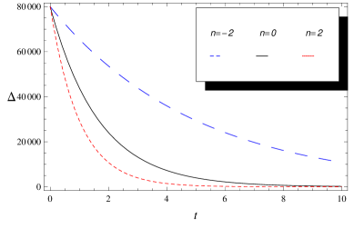
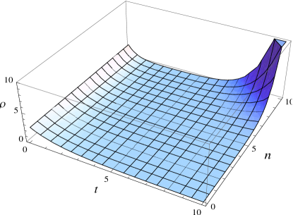
The mean Hubble parameter is found to be constant whereas the directional Hubble parameters are dynamical. For $n>-3$, $H_{x}$ and $H_{y}$ become constant at $t=0$ as well as for $t\rightarrow{\infty}$. These parameters vary from $H$ by some constant at $t=0$ and coincide for later times of the universe. As the constant being positive (negative), it would increase (decrease) expansion on the $x$-axis and it decreases (increases) expansion on $y$ and $z$ axes. For $n=-3$, $H_{x}$ will increase from $H$ by a constant factor $\frac{2k}{3\alpha}$, while parameters $H_{y}$, $H_{z}$ will decrease by a factor $\frac{k}{3\alpha}$. The anisotropy parameter of expansion is found to be finite for earlier times of the universe and vanishes as $t\rightarrow{\infty}$ for $n>-3$. The plot of $\triangle$ versus cosmic time $t$ is shown in Figure 1.

The deceleration parameter, expansion and shear scalars are given by

$$q=-1,\quad\theta=3l=3H,\quad\sigma^{2}=\frac{k^{2}}{3\alpha^{2}}e^{-2(n+3)lt}.$$ (26)

The volume $V$ of the universe is an exponential function which expands with the increase in time and becomes infinitely large for later times of the universe. Also, the expansion scalar is constant for all times and hence the model would favor the uniform expansion. The deceleration parameter $(q=-1)$ allows the existence of accelerating model for this case which is in agreement with the current observations of SNeIa and CMB^1-2).

Using Eqs.(25) in Eqs.(2)-(14), we obtain the following relation of energy density and pressure

$$\rho+p=\frac{-1}{3\alpha(8\pi+\lambda)}\left[2k^{2}e^{nlt-2(n+3)lt}+3b_{1}e^{nlt}\right],$$ (27)

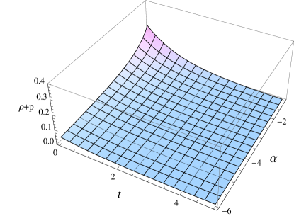
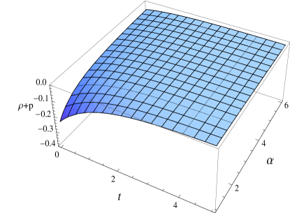
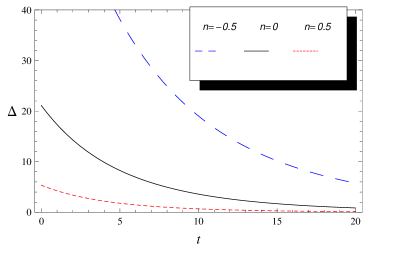
where $b_{1}=n(n-1)l^{2}\alpha^{2}$. This shows that the null energy condition (NEC) is violated, i.e., $\rho+p<0$ which implies that $\omega<-1$. Matter component with $\omega<-1$ is named as ”phantom energy” and is a possible candidate of the present accelerated expansion. The phantom regime favors recent observational cosmology of accelerated cosmic expansion. The behavior of NEC for different values of $\alpha$ is displayed in Figure 2, which shows that NEC is violated for positive values of $\alpha$. Thus, we assume $\alpha>0$ for phantom universe. Equation (27) implies the following dynamical variables of the perfect fluid

Figure 2: Evolution of NEC for $n=2$. The left graph shows that NEC is satisfied for $\alpha<0$ and it is violated for $\alpha>0$ at the right side. We set $l=\lambda=0.1$ and $k=3$. (Colour online)

$$\rho=\frac{-1}{3\alpha(1+\omega)(8\pi+\lambda)}\left[2k^{2}e^{nlt-2(n+3)lt}+3b_{1}e^{nlt}\right],$$ (28)

$$p=\frac{-\omega}{3\alpha(1+\omega)(8\pi+\lambda)}\left[2k^{2}e^{nlt-2(n+3)lt}+3b_{1}e^{nlt}\right].$$ (29)

For the phantom evolution of the universe, $\rho$ decreases with cosmic time and approaches to zero as $t\rightarrow{\infty}$ in the range of $-6<n\leq 0$. When $n<-6$, $\rho$ increases as time goes from zero to infinity and hence diverges. Figure 3 shows that $\rho$ decreases for $n=-1,-4$ and becomes uniform for $n=-6$. However, the value of $n=-7$ shows increasing $\rho$ for the future evolution of the universe. If $n>0,~{}\rho$ decreases with time but for large values of $n$, it shows bouncing behavior as shown in Figure 3. For this model, the scalar curvature $R$ and $f(R,T)$ are given by

$$R = -\frac{2}{3\alpha^{2}}\left[18l^{2}\alpha^{2}+k^{2}e^{-2(n+3)lt}\right],$$

$$f(R,T) = \frac{\alpha}{2}(R+3l(n^{2}l+3))e^{nlt}+\frac{8\pi(1-3\omega)+\lambda(1-\omega)}{6\alpha(8\pi+\lambda)(1+\omega)}$$

$$\times (2k^{2}e^{-(n+6)lt}+3b_{1}e^{nlt}).$$

Figure 3: The left graph shows the behavior of $\rho$ for $-6<n\leq 0$ and $n<-6$, while the right graph presents the evolution of $\rho$ for $n>0$. We set $l=\lambda=0.1$, $k=3$ and $\alpha=0.05$. (Colour online)

3.2 Perfect Fluid Model When $m\neq 0$

For $m\neq 0$, the spatial volume is given by Eq.(21) and the corresponding deceleration parameter is $q=m-1$. If $q>0$, the model represents decelerating universe whereas $q<0$ indicates inflation. To obtain the accelerated expansion model, we take $m<1$. Solving the field equations (2)-(14), the scale factors are found to be

$$A=c_{4}^{2/3}(mlt+c_{2})^{1/m}e^{\frac{2k}{3{\alpha}l(m-n-3)}(mlt+c_{2})^{1-\frac{n+3}{m}}},$$

$$B=c_{4}^{-1/3}(mlt+c_{2})^{1/m}e^{\frac{k}{3{\alpha}l(n-m+3)}(mlt+c_{2})^{1-\frac{n+3}{m}}}.$$ (30)

We discuss the evolution of the scale factors for two cases, i.e., $m>n+3$ and $m<n+3$ along with $0<m<1$. If $m>n+3$, the scale factor $A$ increases with time whereas $B$ tends to zero. For $m<n+3$, the behavior of scale factors is almost identical provided that $n$ is always greater than $-3$ to keep $m$ positive. Substituting Eq.(30) in Eq.(17), we get

$$H=l(mlt+c_{2})^{-1},\quad H_{x}=l(mlt+c_{2})^{-1}+\frac{2k}{3\alpha}(mlt+c_{2})^{-\frac{n+3}{m}},$$ (31)

$$H_{y}=H_{z}=l(mlt+c_{2})^{-1}-\frac{k}{3\alpha}(mlt+c_{2})^{-\frac{n+3}{m}},$$ (32)

$${\Delta}=\frac{2k^{2}}{9l^{2}{\alpha}^{2}}(mlt+c_{2})^{-2\frac{(n+3)}{m}}.$$ (33)

Figure 4: Plot of $\Delta$ versus cosmic time $t$ for different values of $n$. We set $l=0.1$, $k=c_{2}=3$, $m=0.9$ and $\alpha=0.05$. (Colour online)

The Hubble parameters $H,~{}H_{x},~{}H_{y}$ and $H_{z}$ become constant at the initial epoch. As $t\rightarrow{\infty}$, the values of these parameters tend to zero for $n>-3$ and become infinite for $n<-3$.

If $n<-3,~{}\triangle$ increases with cosmic time whereas for $n>-3$, its value decreases and may result to isotropic expansion in future evolution of the universe (see Figure 4). The expansion and shear scalars turn out to be

$$\theta=3l(mlt+c_{2})^{-1},\quad\sigma^{2}=\frac{k^{2}}{3\alpha^{2}}(mlt+c_{2})^{-2\frac{(n+3)}{m}}.$$ (34)

If we replace Eq.(30) in Eqs.(2)-(14), we obtain

$$\rho+p=\frac{-1}{3\alpha(8\pi+\lambda)}\left[2k^{2}(mlt+c_{2})^{-\frac{(n+6)}{m}}+3b_{2}(mlt+c_{2})^{\frac{(n-2m)}{m}}\right],$$ (35)

where $b_{2}=(n(n-1)-m(n+2))l^{2}\alpha^{2}$. $\rho$ and $p$ are obtained as follows

$$\rho=\frac{-1}{3\alpha(1+\omega)(8\pi+\lambda)}\left[2k^{2}(mlt+c_{2})^{-\frac{(n+6)}{m}}+3b_{2}(mlt+c_{2})^{\frac{(n-2m)}{m}}\right],$$ (36)

$$p=\frac{-\omega}{3\alpha(1+\omega)(8\pi+\lambda)}\left[2k^{2}(mlt+c_{2})^{-\frac{(n+6)}{m}}+3b_{2}(mlt+c_{2})^{\frac{(n-2m)}{m}}\right].$$ (37)

Figure 5: Behavior of NEC versus $\alpha$ for $n=3$. The left part shows that NEC is satisfied for $\alpha<0$, while it is violated for $\alpha>0$ shown on the right side. We set $l=\lambda=0.1$, $k=c_{2}=3$ and $m=0.9$. (Colour online)

Figure 6: This figure is plotted for $n=2$. The left part shows that NEC is violated for $\alpha<0$, whereas NEC is satisfied for $\alpha>0$ shown on right side. We set $l=\lambda=0.1$, $k=c_{2}=3$ and $m=0.9$. (Colour online)

Figure 7: Plot of $\rho$ versus cosmic time $t$ for $n\geq 0$. We set $l=\lambda=0.1$, $k=c_{2}=3$, $m=0.9$ and $\alpha=0.05$. (Colour online)

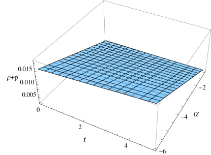
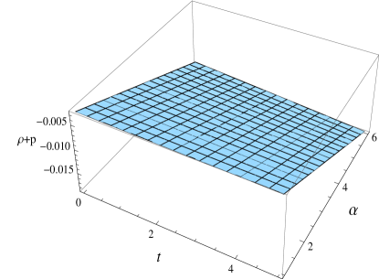
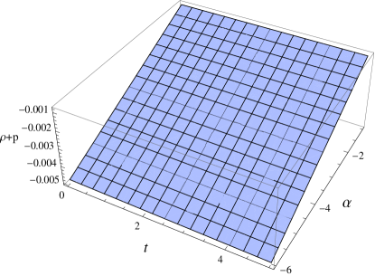
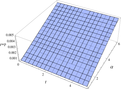
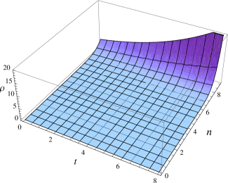
Equation (35) shows that NEC is violated for the power law expansion model. The behavior of NEC is shown in Figures 5-6 which depends on the choice of $\alpha$ as well as $n$. For each value of $n$ except $2\leq{n}\leq 0$, NEC can be satisfied for $\alpha<0$ but the choice $\alpha>0$ does not support it. If $2\leq{n}\leq 0$, the constraints to satisfy and violate NEC are interchanged (see Figure 6). For $m<1$, energy density decreases in the range of $-6<n\leq 0$ and increases with cosmic time $t$ for $n>-7$. For $n>0$, the behavior of $\rho$ is shown in Figure 7. From Eqs.(6) and (15), the Ricci scalar $R$ and $f(R,T)$ are given by

$$R = \frac{2}{3\alpha^{2}}\left[9l^{2}\alpha^{2}(m-2)(mlt+c_{2})^{-2}-k^{2}(mlt+c_{2})^{-2(\frac{n+3}{m})}\right],$$

$$f(R,T) = \frac{\alpha}{2}\left[R(mlt+c_{2})^{\frac{n}{m}}+3n(n-m)l^{2}(mlt+c_{2})^{\frac{n}{m}-2}\ \right.$$

$$+ \left.9l(mlt+c_{2})^{\frac{n}{m}-1}\right]+\frac{8\pi(1-3\omega)+\lambda(1-\omega)}{6\alpha(8\pi+\lambda)(1+\omega)}(2k^{2}(mlt+c_{2})^{-\frac{n+6}{m}}$$

$$+ 3b_{2}(mlt+c_{2})^{\frac{n}{m}-2}).$$

4 Massless Scalar Field Models

The Lagrangian for massless scalar field $\phi$ is given by²⁰⁾

$$\mathcal{L}_{m}=-\frac{1}{2}g^{\mu\nu}\partial_{\mu}\phi\partial_{\nu}\phi,$$ (38)

and the corresponding energy-momentum tensor is

$$T_{{\mu}{\nu}}=\partial_{\mu}\phi\partial_{\nu}\phi-\frac{1}{2}g_{\mu\nu}\partial_{\gamma}\phi\partial^{\gamma}\phi.$$ (39)

Here, $T_{{\mu}{\nu}}$ represents stiff matter with EoS $\omega_{\phi}=1$. Using Eqs.(7), (9) and (39), we obtain the following field equations for massless scalar field

$$\left(\frac{\ddot{A}}{A}+2\frac{\ddot{B}}{B}-2\frac{\dot{A}\dot{B}}{AB}-2\frac{\dot{B}^{2}}{B^{2}}\right)F+\frac{3}{2}\ddot{F}-\frac{1}{2}\left(\frac{\dot{A}}{A}+2\frac{\dot{B}}{B}\right)\dot{F}=-\frac{3}{2}(8\pi+\lambda)\dot{\phi}^{2},$$ (40)

$$\left(\frac{\ddot{A}}{A}-2\frac{\ddot{B}}{B}+2\frac{\dot{A}\dot{B}}{AB}-2\frac{\dot{B}^{2}}{B^{2}}\right)F-\frac{1}{2}\ddot{F}+\left(\frac{3}{2}\frac{\dot{A}}{A}-\frac{\dot{B}}{B}\right)\dot{F}=\frac{1}{2}(8\pi+\lambda)\dot{\phi}^{2},$$ (41)

$$\left(\frac{\dot{B}^{2}}{B^{2}}-\frac{\ddot{A}}{A}\right)F-\frac{1}{2}\ddot{F}-\frac{1}{2}\left(\frac{\dot{A}}{A}-2\frac{\dot{B}}{B}\right)\dot{F}=\frac{1}{2}(8\pi+\lambda)\dot{\phi}^{2}.$$ (42)

Figure 8: Evolution of $\phi$ versus cosmic time $t$ for $m=0$ and different values of $n$: solid(black) $n=1$; dashed(red), $n=0$; dahsed(blue), $n=-1$. We set $l=\lambda=0.1$, $k=3$ and $\alpha=0.05$. (Colour online)

4.1 Scalar Field Models When $m=0$ and $m\neq 0$

The field equations with massless scalar field are similar to the perfect fluid case with $\rho_{\phi}+p_{\phi}=\dot{\phi}^{2}$. Hence, we obtain the same results for the scale factors and other physical parameters. Substituting Eq.(25) in (40)-(42), we obtain the time derivative of scalar field $\phi$ as

$$\dot{\phi}=\pm\sqrt{\frac{-1}{3\alpha(8\pi+\lambda)}\left[2k^{2}e^{nlt-2(n+3)lt}+3b_{1}e^{nlt}\right]}.$$ (43)

Using Eqs.(25) and (43) in (6), it follows that

$$f(R,T)=\frac{\alpha}{2}(R+3l(n^{2}l+3))e^{nlt}-\frac{4\pi}{3\alpha(8\pi+\lambda)}(2k^{2}e^{-(n+6)lt}+3b_{1}e^{nlt}).$$ (44)

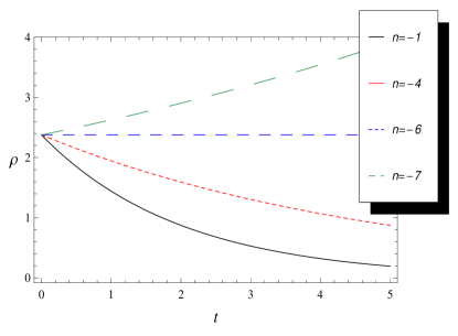
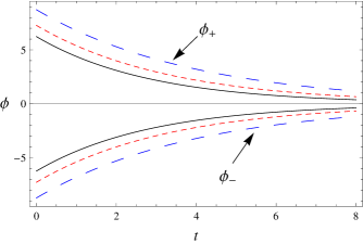
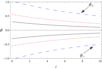
The behavior of $\phi$ for exponential expansion is shown in Figure 8. If we solve Eqs.(40)-(42) for the case $m\neq 0$, we get the similar solutions as given in section 2.2. The expression of $\dot{\phi}$ is obtained as follows

$$\dot{\phi}=\pm\sqrt{\frac{-1}{3\alpha(8\pi+\lambda)}\left[2k^{2}(mlt+c_{2})^{-\frac{(n+6)}{m}}+3b_{2}(mlt+c_{2})^{\frac{(n-2m)}{m}}\right]}.$$ (45)

Evolution of $\phi$ versus cosmic time $t$ for different values of $n$ is shown in Figure 9. Substituting Eqs.(30) and (45) in Eq.(6), we have

$$f(R,T)=\frac{\alpha}{2}\left[R(mlt+c_{2})^{\frac{n}{m}}+3n(n-m)l^{2}(mlt+c_{2})^{\frac{n}{m}-2}\ +9l\right.$$

$$\times \left.(mlt+c_{2})^{\frac{n}{m}-1}\right]-\frac{4\pi}{3\alpha(8\pi+\lambda)}\left[2k^{2}(mlt+c_{2})^{-\frac{n+6}{m}}+3b_{2}(mlt+c_{2})^{\frac{n}{m}-2}\right].$$

Figure 9: Evolution of $\phi$ versus cosmic time $t$ for $m\neq 0$ and different values of $n$: solid(black) $n=1$; dashed(red), $n=0$; dahsed(blue), $n=-1$. We set $l=\lambda=0.1$, $k=c_{2}=3$, $m=0.9$ and $\alpha=0.05$. (Colour online)

5 Discussion and Conclusion

The issue of accelerated expansion of the universe can be explained by taking into account the modified theories of gravity such as $f(R,T)$ gravity²³⁾. In $f(R,T)$ gravity, cosmic acceleration may result not only due to geometric contribution to the matter but it also depends on matter contents of the universe. The coupling between matter and geometry in this gravity results in nongeodesic motion of test particles and an extra acceleration is always present. This theory can be applied to explore several issues of current interest and may lead to some significant results as compared to other modified theories.

The homogeneous and anisotropic Bianchi universe models with perfect fluid have been investigated in the context of $f(R,T)$ gravity¹⁴⁾. The exact solution of the field equations are obtained for the particular choice $f(R,T)=R+2f(T)$ with $f(T)={\lambda}T$. The results of this formulation are very similar to that in general relativity and cannot imply the reconstruction of $f(R,T)$ gravity¹⁴⁾. Houndjo¹⁵⁾ used a more general form $f(R,T)=f(R)+{\lambda}T$ to reconstruct the $f(R,T)$ gravity from holographic DE numerically. In present work, we have employed this choice to reconstruct some explicit models of $f(R,T)$ gravity for BI universe. We have presented the phantom evolution of the universe by examining the NEC.

The exact solutions of the modified field equations are obtained for the spatially homogeneous and anisotropic LRS BI universe with perfect fluid and massless scalar field. The law of variation of mean Hubble parameter is assumed which implies two cosmological models for $m=0$ and $m\neq 0$. These models represent the accelerated expansion of the universe which supports the observations of WMAP data and SNeIa^1-2). We have presented physical properties of the models as well as kinematical parameters. In the following, we summarize the results for these two models.

• Model for $V=c_{1}e^{3lt}$

For exponential expansion model, the accelerated expansion of the universe may occur since $q=-1$. The kinematical paramters have been discussed for two cases $n>-3$ and $n<-3$. The expansion scalar is constant, while the Ricci scalar approaches to constant value as $t\rightarrow{\infty}$ for $n>-3$ and take infinitely large values for $n<-3$. The anisotropy parameter of expansion depends on time and vanishes in future evolution for $n>-3$. If $\alpha>0$, NEC is violated. In our discussion, we have considered a particular model of $f(R,T)$ gravity, $f(R,T)=f(R)+\lambda{T}$. We are not able to find the explicit function of $f(R,T)$ by using Eq.(6). For $\lambda=0$, we develop $f(R)$ in terms of $R$ and hence the function $f(R,T)$ as

$$f(R)=\left[\frac{2{\alpha}\omega}{1+\omega}(R+12H^{2})+\frac{1}{2\alpha}\{3{\alpha}^{2}H((n^{2}-4)H+3)\right.+\left.\frac{1-3\omega}{1+\omega}b_{1}\}\right]e^{nlt},$$

which can be expressed as

$$f(R_{1})=const_{1}\times{R_{1}}^{m_{1}}+const_{2}\times{R_{1}}^{m_{2}},$$

where $R_{1}=R+12H^{2},~{}m_{1}=\frac{n+6}{2(n+3)}$ and $m_{2}=m_{1}-1$. The models of $f(R_{1})$ depending on $n$ are shown in table 1. We find that:

Table 1: Models of $f(R_{1})$ corresponding to $n$.

$n$			$f(R_{1})$
$n=0$			$R_{1}+R^{0}_{1}$, $R_{1}^{0}=const$
$n=-2$			$R_{1}+R_{1}^{2}$
$n=-6$			$R_{1}^{0}+\frac{1}{R_{1}}$
$n=-4$			$R_{1}^{-1}+R_{1}^{-2}$
$n=-\frac{12}{5}$			$R_{1}^{3}+R_{1}^{2}$
$n=-\frac{18}{5}$			$R_{1}^{-2}+R_{1}^{-3}$
$n=-\frac{3}{2}$			$R_{1}^{\frac{3}{2}}+R_{1}^{\frac{1}{2}}$
$n=-\frac{9}{2}$			$R_{1}^{\frac{-1}{2}}+R_{1}^{\frac{-3}{2}}$

For $n=0,~{}f(R)$ represents the $\Lambda$CDM model, i.e., $f(R)=R+\Lambda$. If we put $constant=0$, then $f(R,T)$ is of the form $f(R,T)=R+T$. The most famous Starobinsky’s model²⁴⁾, $f(R)=R+\alpha{R}^{2}$ is achieved for $n=-2$ and the corresponding $f(R,T)$ function is $f(R,T)=R+\alpha{R}^{2}+T$. For $n=-6$, $f(R,T)$ can be presented as $f(R,T)=\frac{1}{R}+T$.

For massless scalar field $(m=0)$, we have found similar results for scale factors as in perfect fluid. The expression of $f(R)$ is

$$f(R)=\left[{\alpha}(R+12H^{2})+\frac{1}{2\alpha}\{3{\alpha}^{2}H((n^{2}-4)H+3)-b_{1}\}\right]e^{nlt}.$$

i.e., $f(R_{1})=const_{3}\times{R_{1}}^{m_{1}}+const_{4}.\times{R_{1}}^{m_{2}}$.

• Model for $V=(mlt+c_{2})^{3/m}$

For $m\neq 0$, the deceleration parameter is $q=m-1$, which leads to the accelerating universe model for $0<m<1$ and if $m>1(q>0)$, the model represents decelerating phase of the universe. The evolution of the scale factors is discussed for two cases $m>n+3$ and $m<n+3$ with $0<m<1$. The anisotropy parameter of expansion increases for $n<-3$, whereas it may result in isotropic expansion in future evolution of the universe for $n>-3$. The Hubble parameter, expansion scalar and shear scalar approach to constant at earlier times of the universe and approach to zero as $t\rightarrow{\infty}$. The scalar curvature $R$ becomes constant as $t\rightarrow{\infty}$ for $n>-3$, whereas it diverges for $n<-3$. For $\lambda=0$, we have

$$f(R) = (mlt+c_{2})^{n/m}\left[\frac{2{\alpha}\omega}{1+\omega}(R-6(m-2)H^{2})+\frac{\alpha}{2}H\{3H(n^{2}\right.$$

$$+ \left.m-4)+\frac{1-3\omega}{\alpha^{2}l^{2}(1+\omega)}b_{2}H+9\}\right]$$

which results in

$$f(R_{2})=const_{5}\times{R_{2}}^{m_{1}}+const_{6}\times{R_{2}}^{m_{2}},$$

where $R_{2}=R-6(m-2)H^{2}$. In case of massless scalar field, $f(R)$ is

$$f(R) = (mlt+c_{2})^{n/m}\left[\alpha(R-6(m-2)H^{2})+\frac{\alpha}{2}H\{3H(n^{2}+m\right.$$

$$- \left.4)+\frac{b_{2}H}{\alpha^{2}l^{2}}+9\}\right],$$

i.e., $f(R_{2})=const_{7}\times{R_{2}}^{m_{1}}+const_{8}\times{R_{2}}^{m_{2}}$. The scalar field $\phi$ is found to be decreasing function of cosmic time (see Figures 8, 9)¹⁹⁾.

We have seen that all $f(R)$ represent identical behavior with different constraints. The NEC is found to be violated for both models $m=0$ and $m\neq 0$ which results in phantom evolution. For ${\omega}<-1$, energy density is found to be positive and pressure is negative. Thus, our solutions for perfect fluid represent the phantom era of DE which are consistent with present observations of WMAP5²⁵⁾. The isotropic behavior of models is observed for future evolution. It can be concluded that solutions of massless scalar field in $f(R,T)$ gravity can be recovered for both exponential and power law expansion models from phantom solutions of perfect fluid if $\omega=1$.

Acknowledgment

We would like to thank the anonymous referee for fruitful comments.

1) C. L. Bennett, M. Halpern, G. Hinshaw, N. Jarosik, A. Kogut, M. Limon, S. S. Meyer, L. Page, D. N. Spergel, G. S. Tucker, E. Wollack, E. L. Wright, C. Barnes, M. R. Greason, R. S. Hill, E. Komatsu, M. R. Nolta, N. Odegard, H. V. Peiris, L. Verde and J. L. Weiland: Astrophys. J. Suppl. 148 (2003) 1; D. N. Spergel, L. Verde, H. V. Peiris, E. Komatsu, M. R. Nolta, C. L. Bennett, M. Halpern, G. Hinshaw, N. Jarosik, A. Kogut, M. Limon, S. S. Meyer, L. Page, G. S. Tucker, J. L. Weiland, E. Wollack and E. L. Wright: Astrophys. J. Suppl. 148 (2003) 175; D. N. Spergel, R. Bean, O. Dor , M. R. Nolta, C. L. Bennett, J. Dunkley, G. Hinshaw, N. Jarosik, E. Komatsu, L. Page, H. V. Peiris, L. Verde, M. Halpern, R. S. Hill, A. Kogut, M. Limon, S. S. Meyer, N. Odegard, G. S. Tucker, J. L. Weiland, E. Wollack and E. L. Wright: Astrophys. J. Suppl. 170 (2007) 377.
 2) S. Perlmutter, S. Gabi, G. Goldhaber, A. Goobar, D. E. Groom, I. M. Hook, A. G. Kim, M. Y. Kim, G. C. Lee, R. Pain, C. R. Pennypacker, I. A. Small, R. S. Ellis, R. G. McMahon, B. J. Boyle, P. S. Bunclark, D. Carter, M. J. Irwin, K. Glazebrook, H. J. M. Newberg, A. V. Filippenko, T. Matheson, M. Dopita and W. C. Couch: Astrophys. J. 483 (1997) 565; S. Perlmutter, G. Aldering, M. D. Valle, S. Deustua, R. S. Ellis, S. Fabbro, A. Fruchter, G. Goldhaber, A. Goobar, D. E. Groom, I. M. Hook, A. G. Kim, M. Y. Kim, R. A. Knop, C. Lidman, R. G. McMahon, P. Nugent, R. Pain, N. Panagia, C. R. Pennypacker, P. Ruiz-Lapuente, B. Schaefer and N. Walton: Nature 391 (1998) 51; S. Perlmutter, G. Aldering, G. Goldhaber, R. A. Knop, P. Nugent, P. G. Castro, S. Deustua, S. Fabbro, A. Goobar, D. E. Groom, I. M. Hook, A. G. Kim, M. Y. Kim, J. C. Lee, N. J. Nunes, R. Pain, C. R. Pennypacker, R. Quimbey, C. Lidman, R. S. Ellis, M. Irwin, R. G. Mcmahon, P. Ruiz-lapuente, N. Walton, B. Schaefer, B. J. Boyle, A. V. Filippenko, T. Matheson, A. S. Fruchter, N. Panagia, H. J. M. Newberg and W. J. Couch: Astrophys. J. 517 (1999) 565; A. G. Riess, L. G. Strolger, J. Tonry, Z. Tsvetanov, S. Casertano, H. C. Ferguson, B. Mobasher, P. Challis, N. Panagia, A. V. Filippenko, W. Li, R. Chornock, R. P. Kirshner, B. Leibundgut, M. Dickinson, A. Koekemoer, N. A. Grogin and M. Giavalisco : Astrophys. J. 607 (2004) 665; A. G. Riess, L. G. Strolger, S. Casertano, H. C. Ferguson, B. Mobasher, B. Gold, P. J. Challis, A. V. Filippenko, S. Jha, W. Li, J. Tonry, R. Foley, R. P. Kirshner, M. Dickinson, E. MacDonald, D. Eisenstein, M. Livio, J. Younger, C. Xu, T. Dahl n and D. Stern : Astrophys. J. 659 (2007) 98.
 3) E. Hawkins, S. Maddox, S. Cole, O. Lahav, D. S. Madgwick, P. Norberg, J. A. Peacock, I. K. Baldry, C. M. Baugh, J. Bland-Hawthorn, T. Bridges, R. Cannon, M. Colless, C. Collins, W. Couch, G. Dalton, R. D. Propris, S. P. Driver, S.P., G. Efstathiou, R. S. Ellis, C.S. Frenk, K. Glazebrook, C. Jackson, B. Jones, I. Lewis, S. Lumsden, W. Percival, B. A. Peterson, W. Sutherland and K. Taylor: Mon. Not. Roy. Astron. Soc. 346 (2003) 78; M. Tegmark, M. A. Strauss, M. R. Blanton, K. Abazajian, S. Dodelson, H. Sandvik, X. Wang, D. H. Weinberg, I. Zehavi, N. A. Bahcall, F. Hoyle, D. Schlegel, R. Scoccimarro, M. S. Vogeley, A. Berlind, T. Budavari, A. Connolly, D. J. Eisenstein, D. Finkbeiner, J. A. Frieman, J. E. Gunn, L. Hui, B. Jain, D. Johnston, S. Kent, H. Lin, R. Nakajima, R. C. Nichol, J. P. Ostriker, A. Pope, R. Scranton, U. Seljak, R. K. Sheth, A. Stebbins, A. S. Szalay, I. Szapudi, Y. Xu, J. Annis, J. Brinkmann, S. Burles, F. J. Castander, I. Csabai, J. Loveday, M. Doi, M. Fukugita, B. Gillespie, G. Hennessy, D. W. Hogg, Z. E. Ivezic , G. R. Knapp, D. Q. Lamb, B. C. Lee, R. H. Lupton, T. A. McKay, P. Kunszt, J. A. Munn, L. Connell, J. Peoples, J. R. Pier, M. Richmond, C. Rockosi, D. P. Schneider, C. Stoughton, D. L. Tucker, D. E. V. Berk, B. Yanny and D. G. York: Phys. Rev. D 69 (2004) 103501; S. Cole , W. J. Percival, J. A. Peacock, P. Norberg, C. M. Baugh, C. S. Frenk, I. Baldry, J. B. Hawthorn, T. Bridges, R. Cannon, M. Colless, C. Collins, W. Couch, N. J. G. Cross, G. Dalton, V. R. Eke, R. D. Propris, S. P. Driver, G. Efstathiou, R. S. Ellis, K. Glazebrook, C. Jackson, A. Jenkins, O. Lahav, I. Lewis, S. Lumsden, S. Maddox, D. Madgwick, B. A. Peterson, W. Sutherland and K. Taylor: Mon. Not. Roy. Astron. Soc. 362 (2005) 505.
 4) D. J. Eisentein, I. Zehavi, D. W. Hogg, R. Scoccimarro, M. R. Blanton, R. C. Nichol, R. Scranton, Hee-Jong Seo, M. Tegmark, Z. Zheng, S. F. Anderson, J. Annis, N. Bahcall, J. Brinkmann, S. Burles, F. J. Castander, A. Connolly, I. Csabai, M. Doi, M. Fukugita, J. A. Frieman, K. Glazebrook, J. E. Gunn, J. S. Hendry, G. Hennessy, Z. Ivezic’, S. Kent, G. R. Knapp, H. Lin, Yeong-Shang Loh, R. H. Lupton, B. Margon, T. A. McKay, A. Meiksin, J. A. Munn, A. Pope, M. W. Richmond, D. Schlegel, D. P. Schneider, K. Shimasaku, C. Stoughton, M. A. Strauss, M. SubbaRao, A. S. Szalay, I. Szapudi, D. L. Tucker, B. Yanny, and D. G. York: Astrophys. J. 633 (2005) 560.
 5) B. Jain and A. Taylor: Phys. Rev. Lett. 91 (2003) 141302.
 6) P. Astier J. Guy, N. Regnault, R. Pain, E. Aubourg, D. Balam, S. Basa, R. G. Carlberg, S. Fabbro, D. Fouchez, I. M. Hook, D. A. Howell, H. Lafoux, J. D. Neill, N. Palanque-Delabrouille, K. Perrett, C. J. Pritchet, J. Rich, M. Sullivan, R. Taillet, G. Aldering, P. Antilogus, V. Arsenijevic, C. Balland, S. Baumont, J. Bronder, H. Courtois, R. S. Ellis, M. Filiol, A. C. Gon alves, A. Goobar, D. Guide, D. Hardin, V. Lusset, C. Lidman, R. McMahon, M. Mouchet, A. Mourao, S. Perlmutter, P. Ripoche, C. Tao and N. Walton : Astron. Astrophys. 447 (2006) 31; S. Tsujikawa: Lect. Notes Phys. 800 (2010) 99; P. J. E. Peebles: Rev. Mod. Phys. 75 (2003) 559.
 7) V. Sahni: Lect. Notes Phys. 653 (2004) 141; T. Padmanabhan: Gen. Relativ. Gravit. 40 (2008) 529; R. R. Caldwell: Phys. Lett. B 545 (2002) 23; S. Nojiri and S. D. Odintsov: Phys. Lett. B 562 (2003) 147; B. Feng, X. L. Wamg and X. M. Zhang: Phys. Lett. B 607 (2005) 35; A. A. Sen: Phys. Rev. D 66 (2002) 043507; T. Padmanabhan: Phys. Rev. D 66 (2002) 021301.
 8) O. Akarsu and C. B. Kilinc: Gen. Relativ. Gravit. 42 (2010) 1; M. Sharif and M. Zubair: Int. J. Mod. Phys. D 19 (2010) 1957; Astrophys. Space Sci. 330 (2010) 399; ibid. 339 (2012) 45.
 9) S. Nojiri and S. D. Odintsov: Int. J. Geom. Methods Mod. Phys. 4 (2007) 115; T. P. Sotiriou and V. Faraoni: Rev. Mod. Phys. 82 (2010) 451.
 10) R. Ferraro and F. Fiorini: Phys. Rev. D 75 (2007) 084031; G. R. Bengochea and R. Ferraro: Phys. Rev. D 79 (2009) 124019; E. V. Linder: Phys. Rev. D 81 (2010) 127301.
 11) S. M. Carroll, A. De Felice, V. Duvvuri, D. A. Easson, M. Trodden and M. S. Turner: Phys. Rev. D 71 (2005) 063513; G. Cognola, E. Elizalde, S. Nojiri, S. D. Odintsov and S. Zerbini: Phys. Rev. D 73 (2006) 084007.
 12) T. Harko, F. S. N. Lobo, S. Nojiri and S. D. Odintsov: Phys. Rev. D 84 (2011) 024020.
 13) L. D. Landau and E. M. Lifshitz: The Classical Theory of Fields (Butterworth-Heinemann, 2002).
 14) K. S. Adhav: Astrophys. Space Sci. 339 (2012) 365; D. R. K. Reddy, R. Santikumar and R. L. Naidu: Astrophys. Space Sci. DOI: 10.1007/s10509-012-1158-7; R. Chaubey, A.K. Shukla: Astrophys. Space Sci. DOI: 10.1007/s10509-012-1204-5.
 15) M. J. S. Houndjo: Int. J. Mod. Phys. D 21 (2012) 1250003; M. J. S. Houndjo and O. F. Piattella: Int. J. Mod. Phys. D 21 (2012) 1250024; M. Jamil, D. Momeni, M. Raza and R. Myrzakulov: Eur. Phys. J. C 72 (2012) 1999.
 16) M. Sharif and M. Zubair: JCAP 03 (2012) 028 [Errata 05 (2012) E01]; Thermodynamic Behavior of $f(R,T)$ Gravity Models at the Apparent Horizon (To appear in Cent. Eur. J. Phys).
 17) M. Sharif and M. F. Shamir: Class. Quantum Grav. 26 (2009) 235020; Gen. Relativ. Gravit. 42 (2010) 2643.
 18) M. Sharif and H. R. Kausar: Phys. Lett. B 697 (2011) 1.
 19) M. Sharif and W. Saira: Eur. Phys. J. C 72 (2012) 1876; C. Aktas, S. Aygun and I. Yilmaz: Phys. Lett. B 707 (2012) 237.
 20) S. Capozziello: Phys. Lett. B 639 (2012) 135; S. Capozziello and M. Laurentis: Phys. Rep. 509 (2011) 1; D. Yunshuang, Z. Hongsheng and L. Xin-Zhou: Eur. Phys. J. C 71 (2011) 1660; Y. Bisabr: Phys. Lett. B 690 (2011) 456; V. Faraoni: Class. Quantum Grav. 26 (2009) 145014.
 21) M. Sharif and M. Zubair: Astrophys. Space Sci. DOI: 10.1007/s10509-012-1169-4.
 22) M. S. Berman: Nuovo Cimento B 74 (1983) 182; M. S. Berman and F. M. Gomide: Gen. Relativ. Gravit. 20 (1988) 191.
 23) K. Bamba, S. Capozziello, S. Nojiri and S. D. Odintsov: Astrophys. Space Sci. DOI: 10.1007/s10509-012-1181-8.
 24) A. A. Starobinsky: Phys. Lett. B 91 (1980) 99.
 25) E. Komatsu, J. Dunkley, R. Nolta, C. L. Bennett, B. Gold, G. Hinshaw, N. Jarosik, D. Larson, M. Limon, L. Page, D. N. Sperge, M. Halpern, R. S. Hill, A. Kogut, S. S. Meyer, G. S. Tucker, J. L. Weiland, E. Wollack, and E. L. Wright: Astrophys. J. Suppl. 180 (2009) 330.