Spoke-like differential rotation in a convective dynamo with a coronal envelope
Abstract
We report on the results of four convective dynamo simulations with an outer coronal layer. The magnetic field is self-consistently generated by the convective motions beneath the surface. Above the convection zone, we include a polytropic layer that extends to 1.6 solar radii. The temperature increases in this region to times the value at the surface, corresponding to times the value at the bottom of the spherical shell. We associate this region with the solar corona. We find solar-like differential rotation with radial contours of constant rotation rate, together with a near-surface shear layer. This non-cylindrical rotation profile is caused by a non-zero latitudinal entropy gradient that offsets the Taylor–Proudman balance through the baroclinic term. The meridional circulation is multi-cellular with a solar-like poleward flow near the surface at low latitudes. In most of the cases, the mean magnetic field is oscillatory with equatorward migration in two cases. In other cases, the equatorward migration is overlaid by stationary or even poleward migrating mean fields.
Subject headings:
convection – dynamo – magnetohydrodynamics (MHD) – Sun: activity – Sun: rotation – turbulence1. Introduction
The Sun has an activity cycle of 11 yr, which is manifested by sunspots occurring at the solar surface. The sunspot number changes from a few during minimum to over 200 during maximum. The sunspot locations display a latitudinal dependence during the cycle. At solar minimum (maximum), sunspots emerge preferably at higher (lower) latitudes. By plotting the sunspot latitudes for several cycles, one obtains the “butterfly diagram”. Every 11 yr the polarity of sunspot pairs changes sign, which is characteristic of the 22 yr magnetic cycle. To understand this cyclical behavior, one has to connect the fluid motions in the Sun with magnetic field generation to construct dynamo models. These dynamo models should be able to reproduce the 22 yr magnetic activity cycle as well as the large-scale magnetic field evolution at the surface of the Sun. It is widely believed that sunspots are correlated with the large-scale magnetic field distribution. Therefore, a successful solar dynamo model should reproduce the equatorward migration of the large-scale field as we observe it indirectly from sunspots and more directly from synoptic magnetograms.
Until recently, only kinematic mean-field models, where turbulent effects are parameterized through transport coefficients (e.g., Krause & Rädler, 1980), have been able to show equatorward migration (e.g., Dikpati & Charbonneau, 1999; Käpylä et al., 2006; Kitchatinov & Olemskoy, 2012). Such models have been used to reproduce certain features of the solar cycle, such as the Maunder minimum (e.g.,, Karak, 2010). However, those models are only valid in the kinematic regime in which the fluid motions are assumed to be given, so they are not self-consistently generated. The backreaction from the magnetic field is either ignored or taken into account in a rudimentary way involving ad hoc quenching of the turbulent transport coefficients. Until recently, direct numerical simulations (DNS) of the solar dynamo have been unsuccessful in producing migration toward the equator using convective motions to drive a dynamo (e.g., Gilman, 1983; Brun et al., 2004; Käpylä et al., 2010; Ghizaru et al., 2010; Brown et al., 2011; Nelson et al., 2013). This was presumably due to the low fluid and magnetic Reynolds numbers of those simulations. Equatorward migration was, for the first time, found in DNS by Käpylä et al. (2012). The exact cause is not yet fully understood, but the amount of density stratification seems to play an important role (Käpylä et al., 2013).
An important ingredient of the solar dynamo is differential rotation. It is believed that strong shear at the bottom of the convection zone (Spiegel & Weiss, 1980) or near the surface (Brandenburg, 2005), plays an important role in amplifying the magnetic field. However, even today it is not straightforward to reproduce a solar-like differential rotation profile. Mean-field simulations (Brandenburg et al., 1992; Kitchatinov & Rüdiger, 1995) have been able to reproduce a solar-like rotation profile by modeling small-scale effects through mean-field coefficients such as the effect and anisotropic heat transport (see, e.g., Rüdiger, 1980, 1989). These models reproduce the positive (negative) latitudinal gradient of angular velocity in the northern (southern) hemisphere—i.e., the equator rotates faster than the poles—together with “spoke-like” contours in the meridional plane. DNS of convective dynamos are able to reproduce a rapidly rotating equator at sufficiently large Coriolis numbers (Brun et al., 2004; Käpylä et al., 2011b). Spoke-like differential rotation has only been found in purely hydrodynamical large-eddy simulations (LES) by imposing a latitudinal entropy gradient (Miesch et al., 2006) or, recently, by adding a stably stratified layer (Brun et al., 2011) at the bottom of the convection zone. A self-consistently generated spoke-like profile in DNS of magnetohydrodynamics has not yet been found.
An important issue with solar dynamo models is the effect of catastrophic quenching of the dynamo at high magnetic Reynolds numbers; see Brandenburg & Subramanian (2005). This is caused by the accumulation of magnetic helicity in the dynamo region. DNS provide evidence that magnetic helicity fluxes both within and through the boundaries of the dynamo domain can prevent the dynamo from being catastrophically quenched (e.g., Brandenburg & Sandin, 2004; Hubbard & Brandenburg, 2012). In the case of the Sun, magnetic helicity flux can emerge through the solar surface and can be transported away from the Sun by coronal mass ejections or by the solar wind (Blackman & Brandenburg, 2003). In earlier work this was modeled by using an upper layer at the top of a dynamo region to allow for magnetic helicity fluxes leaving the domain (Warnecke & Brandenburg, 2010; Warnecke et al., 2011, 2012a, 2012b). This two-layer model was successful in showing that the dynamo is not only enhanced, but that it can actually trigger the emergence of coronal ejections. These ejections have a similar shape as coronal mass ejections and carry a significant amount of magnetic helicity out of the dynamo region. In these models, the temperature in the coronal layer was the same as at the surface of the convection zone, which did not allow for a large density jump to develop. Furthermore, in the polytropic convection zone of Warnecke et al. (2012b), the convective flux was smaller than the radiative flux. Besides dynamo models, this two-layer approach was successful in combination with stratified turbulence in producing a bipolar magnetic region (Warnecke et al., 2013b) as a possible mechanism of sunspot formation.
In this work we use the two-layer approach to investigate the influence of the coronal layer as an upper boundary condition for a convective dynamo. We focus on the physical properties and dynamics in the convection zone. The effects of varying the strength of stratification on a convective dynamo without a corona is studied in a companion paper (Käpylä et al., 2013).
2. Model and Setup
We use a two-layer model in spherical polar coordinates (), where the lower layer () represents the convection zone and the upper layer represents the corona. The simulations are performed in a spherical wedge with radial extent , where corresponds to the bottom of the convection zone and to the solar radius, for colatitudes and an azimuthal extent . We solve the following equations of compressible magnetohydrodynamics,
| (1) |
| (2) |
| (3) |
| (4) |
where the magnetic field is given by and thus obeys at all times, is the current density, is the vacuum permeability, and are the magnetic diffusivity and kinematic viscosity, respectively, is the advective time derivative, is the density, and is the velocity. The traceless rate-of-strain tensor is given by
| (5) |
where semicolons denote covariant differentiation; see Mitra et al. (2009) for details. Furthermore, is the rotation vector and is the pressure. The gravitational acceleration is given by
| (6) |
where is Newton’s gravitational constant and is the mass of the star. The radiative and sub-grid scale (SGS) heat fluxes are defined as
| (7) |
where is the radiative heat conductivity and is the turbulent heat diffusivity, which represents the unresolved convective transport of heat. The fluid obeys the ideal gas law, , where is the ratio of specific heats at constant pressure and constant volume, respectively, and is the internal energy density, defining the temperature . Finally, is the cooling profile that is specified in Equation (10).
The two-layer model is similar to that used in previous work (Warnecke & Brandenburg, 2010; Warnecke et al., 2011, 2012a, 2012b), except that here we improve the model of Warnecke et al. (2012b) in two important ways. First, we use a more realistic model for the convection zone than in Käpylä et al. (2011a, 2012). Instead of using a polytropic setup with , we lower the radiative flux by using a profile for (defined in Equation (11)) and introducing a turbulent heat conductivity (referred to as in Käpylä et al., 2012). We apply a piecewise constant profile for such that in the interval of it is equal to a quantity (whose value is related to via the Prandtl number specified below), and it goes smoothly to zero above and below the boundaries of the interval. Additionally, we change the temperature profile compared with our earlier isothermal cold corona to a temperature-stratified corona, which is times hotter than the surface and times hotter than the bottom of the convection zone. The profiles of averaged temperature, density, pressure, and entropy for a typical run are shown in Figure 1.
We initialize the simulations with precalculated radial profiles of temperature, density, and pressure. In the convection zone () we have an isentropic and hydrostatic initial state for the temperature, whose gradient is given by
| (8) |
where is the polytropic index for an adiabatic stratification. This leads to a temperature minimum above the surface of the convective layer at . In the corona (), we prescribe the temperature as
| (9) |
where is temperature in the corona, and and the width are chosen to produce a smooth temperature profile as shown in Figure 1. The cooling profile in Equation (4) maintains the temperature profile,
| (10) |
where is a profile function equal to unity in and going smoothly to zero in , and is a cooling luminosity chosen such that the temperature in the corona relaxes towards the reference temperature profile given in Equation (9). As stated in Equation (10), the cooling function is sensitive to the total temperature consisting of a mean part and a fluctuating part. Nevertheless, temperature fluctuations can still develop. The stratification of density follows from hydrostatic equilibrium. The density contrast within the convection zone is (see the sixth column in Table 1), while in the whole domain , where is the density at the bottom (), is the density at the surface () and is the density at the top of the corona (). The location of the surface, , is close to the position where the radial entropy gradient changes sign, which is slightly below the surface; see Figure 1. This implies that, similar to the Sun, convection ceases just below the surface. The radial heat conductivity profile is chosen such that the energy in the convection zone is transported mostly by convective motions. We apply a profile for the viscosity that is constant in the convection zone () and increases smoothly above the surface to a value that is 20 times higher in the corona. This helps to suppress high velocities and sharp flow structures aligned with the rotation vector in the corona—especially in the beginning of the simulation, when the magnetic field is weak. Compared with the use of velocity damping in Warnecke et al. (2012b), this approach is Galilean invariant and allows the flow to develop more freely. The magnetic diffusivity is constant throughout the convection zone, but decreases by 20% in the corona. In the convection zone, the radiative heat conductivity is defined via a polytropic index given by
| (11) |
which has a value of 1.5 at the bottom of the convection zone. The conductivity is proportional to and decreases toward the surface as . In the corona, is chosen such that . The radiative diffusivity varies from at the bottom of the convection zone to near the surface and in the corona. We initialize the magnetic field with weak Gaussian-distributed perturbations inside the convection zone.

We use periodic boundary conditions in the azimuthal direction. For the velocity field we apply stress-free boundary conditions at the radial and latitudinal boundaries. The magnetic field follows a perfect conductor condition at the lower radial and the two latitudinal boundaries. On the outer radial boundary, we force the field to be radial; for a discussion on the applicability of this boundary condition for the Sun, see Warnecke et al. (2012b). We fix the gradient of the temperature at the lower radial boundary such that it corresponds to a given radiative flux and we set the temperature to a constant value at the radial outer boundary. At the latitudinal boundaries, we impose a vanishing -derivative of entropy to have zero heat flux through the boundary.
Our runs are characterized by the values of the fluid and magnetic Reynolds numbers, and , respectively, where is the volume averaged rms velocity in the convection zone, and is used as a reference wavenumber. To represent the turbulent velocities in a proper way, we define , which corrects for the removal of the differential rotation-dominated -component of velocity. In our case, , where is an estimate for the macro-physical turbulent diffusivity. We also define the fluid and magnetic Prandtl numbers and , the Coriolis number , and the Taylor number . Time is given in turnover times, . We measure the magnetic field strength as the rms value over the convection zone, , and we normalize this value with the equipartition value of the magnetic field defined by . The typical diffusion time of the system is characterized by the fluid and magnetic Reynolds numbers times the turnover time. We use the (semi-) turbulent Rayleigh number from the thermally relaxed state of the run,
| (12) |
To monitor the solutions in the convection zone, we use two different heights, one near the surface at , and one in the middle of the convection zone at . We use the Pencil Code111http://pencil-code.googlecode.com with sixth-order centered finite differences in space and a third-order Runge-Kutta scheme in time; see Mitra et al. (2009) for the extension of the Pencil Code to spherical coordinates.
3. Results
| Run | grid | Ta | ||||||||||||
|---|---|---|---|---|---|---|---|---|---|---|---|---|---|---|
| A | ||||||||||||||
| Ab | ||||||||||||||
| Ac | ||||||||||||||
| B |
Note. — The second to sixth columns show quantities that are input parameters to the models, whereas the quantities in the last eight columns are results of the simulations computed from the saturated state. All quantities are volume averaged over the convection zone , unless explicitly stated otherwise. The Mach number is defined as and the latitudinal differential rotation is quantified through evaluated at . is the normalized temperature difference between pole and equator , measured at the surface ().
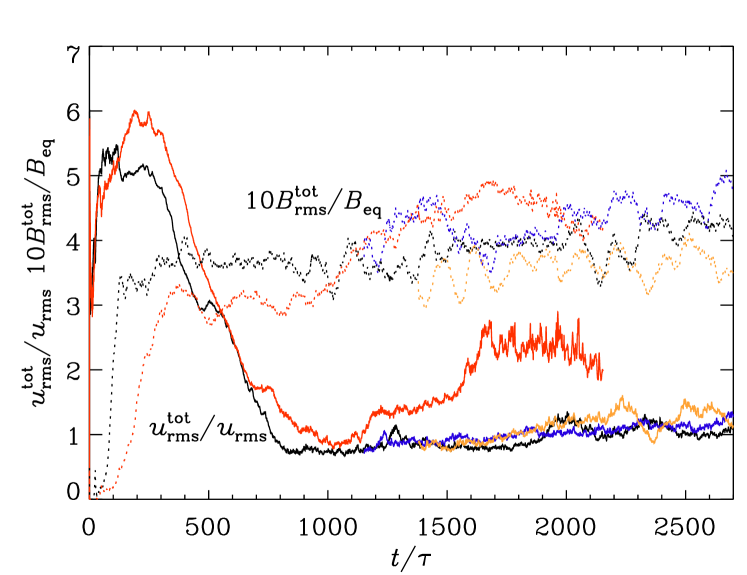
In this work we focus on four simulations that are summarized in Table 1. The main differences between these runs are their rotation rates and the magnetic Reynolds numbers Runs Ab and Ac are a continuation of Run A after and , respectively, but with smaller and higher diffusivities in the convection zone. Runs A, Ab, and Ac have a higher Coriolis number and lower values of than Run B. The Coriolis number of Run A is more than twice that of Run B. However, the nominal rotation rate determined by is only 1.8 times larger. We show the time evolution of the total rms velocity and magnetic field, averaged over the whole domain, and , in all the four runs in Figure 2. Here, the subscripts on angle brackets denote averaging over , , . Convection is sufficiently super-critical to develop during the first few tens of turnover times. After 50–200 turnover times, the dynamo starts to operate and a magnetic field grows at a rate that is higher for faster rotation (compare Runs A and B). Due to the high rotation rate and the lower density in the corona, the velocities there grow to higher values than in the convection zone. As described in Section 2, we use a higher viscosity to suppress these velocities and associated numerical difficulties. After the magnetic field in the convection zone has reached sufficient strength and expanded throughout the whole domain, it quenches the high velocities in the corona significantly, as is evident from Figure 2. When the magnetic field reaches , the rms velocity decreases from to , i.e., the contribution from the corona is now sub-dominant. This is caused by the Lorentz force, which becomes much stronger and comparable to the Coriolis force in the corona. In the saturated state we have , which is reached after around turnover times for Run A. Runs Ab and Ac are restarted from Run A after this saturation point.
For Run B, at first it seems that the saturated state has been reached at , but it turns out that both and the magnetic field start to grow again to reach another saturation level at . While the differential rotation profile remains roughly unchanged despite of the growth of the energies (see Section 3.1), the magnetic field seems to undergo a mode change from an oscillatory to a stationary solution or an oscillatory solution with a much longer period in Run B (see Section 3.4). We note that an increase of in Figure 2, where we show the rms values of the magnetic field computed over the whole domain, does not necessarily imply an increase of the magnetic field inside the convection zone. The increase of the rms magnetic field can also be attributed to the development of magnetic structures ejected from the convection zone into the coronal region.
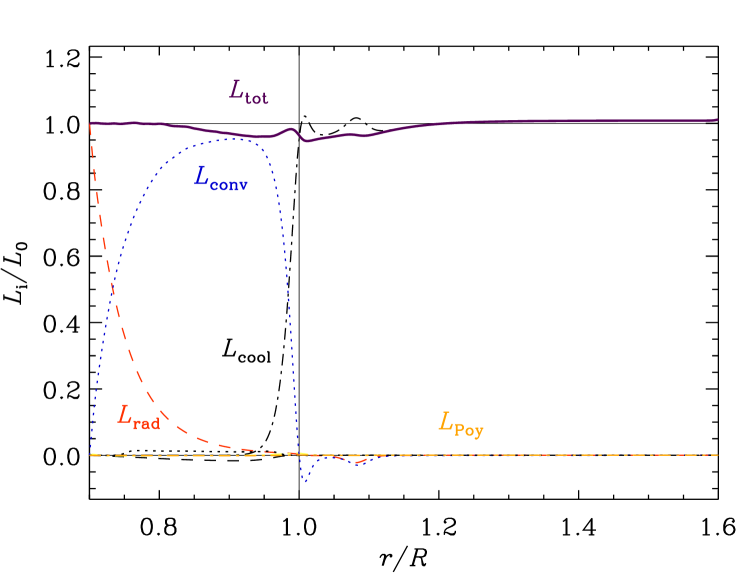
In the upper panel of Figure 3, we show the balance of various radial energy fluxes, contributing to the total luminosity for Run A. The radial components of radiative, convective, kinetic, viscous, and Poynting fluxes, as well as the flux due to the turbulent heat conductivity, are defined as
| (13) | |||||
| (14) | |||||
| (15) | |||||
| (16) | |||||
| (17) | |||||
| (18) |
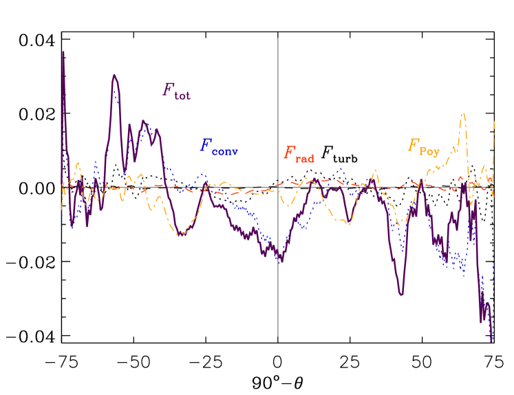
where is the electric field, the primes denote fluctuations, and angle brackets imply averaging over , , and a time interval over which the turbulence is statistically stationary. The resolved convective flux dominates inside the convection zone and reaches much higher values here than in our earlier model (Warnecke et al., 2012b). In the corona the cooling keeps the total flux constant. Note the convective overshoot into the exterior and the negative radiative flux just above the surface (), caused by the higher temperature in the corona. The kinetic energy flux has small negative values in the convection zone. The luminosity due to viscosity and Poynting flux are too small to be visible. In the lower panel of Figure 3, we show the corresponding latitudinal contributions normalized by the rms value of the expected turbulent contribution from the latitudinal entropy gradient, , where . They are generally just a few per cent of the rms value of the turbulent latitudinal heat flux and oriented mostly equatorward (positive in the north and negative in the south). These values are small, indicating that the system is thermally relaxed also in the direction.
3.1. Differential Rotation
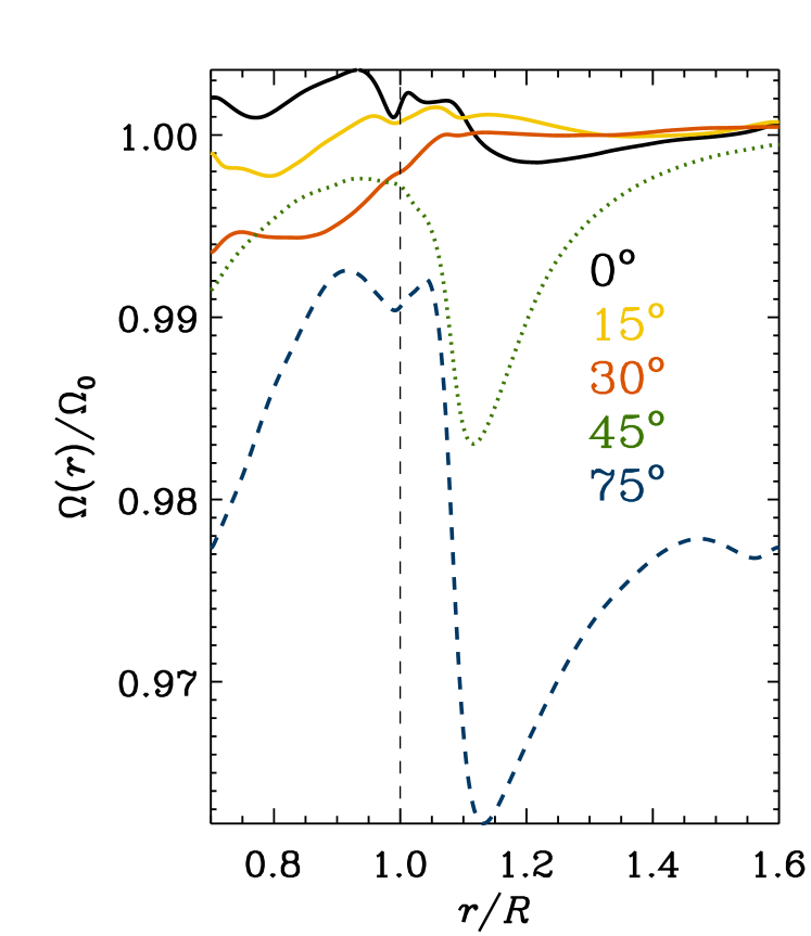
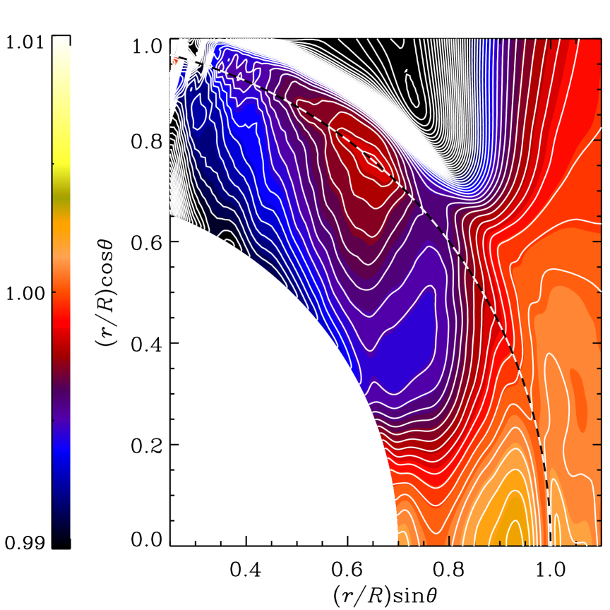
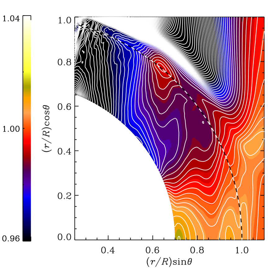
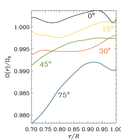
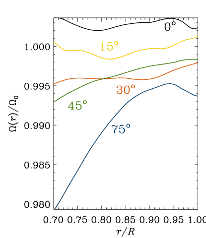
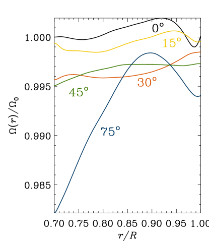
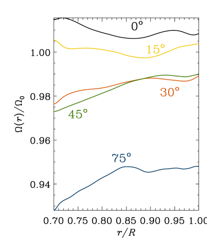
In Figure 4, we show the mean rotation profiles for Runs A and B in the meridional plane and for Runs A, Ab, Ac, and B at four different latitudes. The contours of constant rotation are clearly not cylindrical for any of the four runs. They show a “spoke-like” structure, i.e., the contours are more radial than cylindrical, which is similar to the solar rotation profile obtained by helioseismology (Schou et al., 1998) The equator is rotating faster than the poles, which has been seen in many earlier simulations (Gilman, 1983; Brun et al., 2004; Miesch et al., 2006; Käpylä et al., 2010, 2011b) and resembles the observed rotation of the Sun for our slower rotation case (Run B).
The source of differential rotation is the anisotropy of convection and is described by the and components of the Reynolds stress. Using a suitable parameterization of the Reynolds stress in terms of the effect, one obtains differential rotation where the equator rotates faster than the poles. However, nonlinear mean-field hydrodynamic simulations have shown that for rotation rates comparable with those of the Sun, the contours of constant angular velocity become cylindrical (Brandenburg et al., 1992; Kitchatinov & Rüdiger, 1995). To produce spoke-like rotation contours, the Taylor–Proudman balance has to be overcome by an important contribution in the evolution equation for the mean azimuthal vorticity , which is given by:
| (19) |
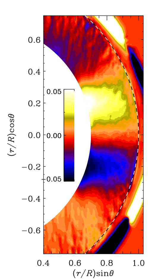
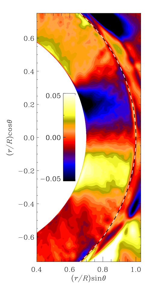
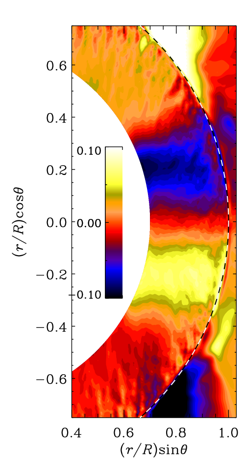
where is the derivative along the rotation axis. The first term in Equation (19) is related to the curl of the Coriolis force and vanishes for cylindrical contours. The second term is the mean baroclinic term, which is caused mainly by latitudinal entropy variations. We ignore here additional contributions such as meridional Reynolds and Maxwell stresses, which turn out to be small. In Figure 5, we plot the first and second terms of Equation (19) for Run A. These two contributions balance each other nearly perfectly. This leads us to conclude that these two terms provides the dominant contribution to the production of mean azimuthal vorticity and that the Taylor–Proudman balance is broken by the baroclinic term. It is remarkable that there is such a large and spatially coherent latitudinal entropy gradient, which is crucial to having a significant azimuthal baroclinic term and is self-consistently produced in the simulations.
Similar results have been obtained in mean-field simulations by including an anisotropic convective heat conductivity (Brandenburg et al., 1992; Kitchatinov & Rüdiger, 1995) or by including a subadiabatic part of the tachocline (Rempel, 2005), and in convection simulations by prescribing a latitudinal entropy gradient at the lower radial boundary of the convection zone (Miesch et al., 2006). More recently, Brun et al. (2011) showed that spoke-like contours can also be obtained by including a lower stably stratified overshoot layer in a purely hydrodynamical simulation.
The right-most panel of Figure 5 shows the mean latitudinal entropy gradient for Run A. The spatial distribution of the gradient agrees with the baroclinic term as well, because in the convection zone, so we can conclude that the dominant contribution in the baroclinic term is due to the product of the latitudinal entropy gradient and the radial temperature gradient, which is more important than the radial entropy gradient multiplying the latitudinal temperature gradient. Compared with Run A, the other three runs, not shown here, have similar (Run B) or even identical (Runs Ab and Ac) distributions of the two terms on the right hand side of Equation (19), as well as the latitudinal entropy gradient. The location of the spoke-like differential rotation profile coincides with a similarly shaped mean latitudinal entropy gradient. The entropy gradient in the northern (southern) hemisphere is negative (positive) below latitude. In Run B, this region reaches to higher latitudes than in Runs A, Ab and, Ac, which leads to radial contours of angular velocity at higher latitudes.
We also note that, owing to the coronal envelope, differential rotation is able to develop a near-surface-shear layer. This is manifested by the concentration of contours of near the surface at lower latitudes for Runs A and B, and is also visible in the other runs as a negative gradient of in the same locations; see Figure 4. In Run B, there also exists a concentration around . In all the simulations, the shear layer is radially more extended than in the Sun and penetrates deeper into the convection zone. Further studies using higher stratification should prove if this is just an artifact of weak stratification. However, the spoke-like rotation profile with strong shear near the surface occurs mostly at lower latitudes (), i.e., close to the equator. At latitudes above , the contours of constant rotation are more complex, but show some indication of strong shear close to the surface and only in Run B do the contours become cylindrical beyond latitude. At higher latitudes (), the near-surface shear layer is again visible.
We were not able to see spoke-like rotation profiles in our previous work (Warnecke et al., 2012b). Therefore, the applied changes might play an important role in the formation of spoke-like profiles. There are three main differences between the two setups. First, the fractional convective flux in Warnecke et al. (2012b) is much lower than in the present setup; compare Figure 2 of Warnecke et al. (2012b) with Figure 3. A stronger convective flux can give rise to more vigorous heat fluxes and thus a more efficient thermal redistribution, causing a more pronounced latitudinal entropy gradient. Second, the temperature in the current setup increases sharply above the surface, generating a hot corona instead of being constant, as in Warnecke et al. (2012b). It is possible that the resulting steep temperature gradient is important in providing enough thermal insulation between the convection zone and the corona. Third, the hot corona leads to a higher density stratification in both the convection zone and the corona.
As seen in Figure 6, the corona rotates nearly uniformly with at lower latitudes (). We suggest that the magnetic field, which connects the surface with the corona, is responsible for this. Near the poles (), the rotation rate drops sharply above the surface (). This drop coincides with the steep temperature and density gradients above the surface, but also with the increase in the applied viscosity profile. Further outside and away from this drop, the rotation profile is cylindrical at high latitudes. This behavior is similar in all four runs.
3.2. Connection with Anisotropic Turbulent Diffusivity Tensor
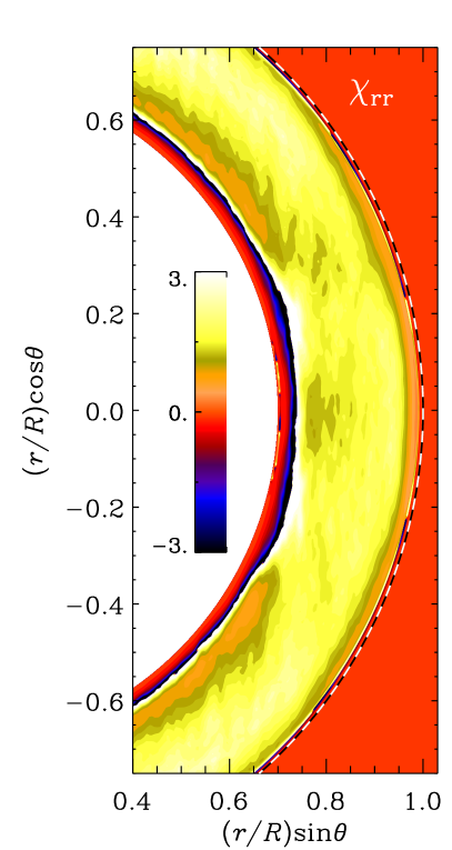
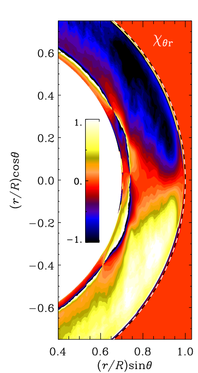
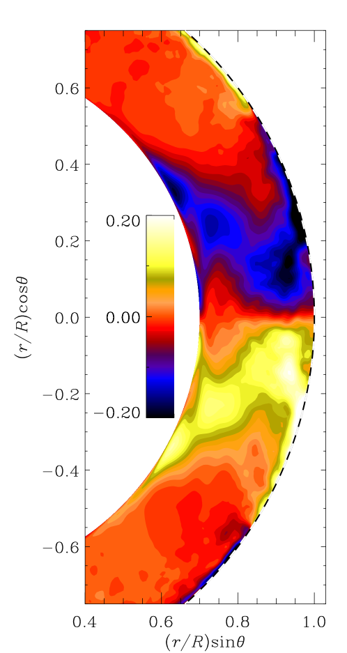
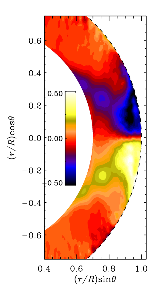
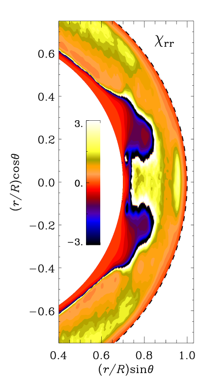
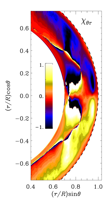
As discussed above, we expect the latitudinal entropy gradient to be a consequence of an anisotropic convective (turbulent) diffusivity tensor. Such anisotropies are caused by the rotational influence on the turbulence (see, e.g.,, Weiss, 1965; Rüdiger, 1989). In particular, there is a term proportional to , where, is the th component of , which gives a symmetric contribution proportional to , so it vanishes at the poles and at the equator. In the presence of a latitudinal entropy gradient, it leads to an additional contribution to the radial convective flux,
| (20) |
Since , and since there is a radial entropy gradient, it also leads to a contribution in the latitudinal flux,
| (21) |
If we were to ignore the second term proportional to , we could estimate by measuring
| (22) |
so
| (23) |
The result is shown in Figure 7, where we also plot a similar estimate of the radial component,
| (24) |
We normalize by and find and , corresponding to and . So, the SGS energy flux is small compared with the resolved turbulent energy flux, as expected.
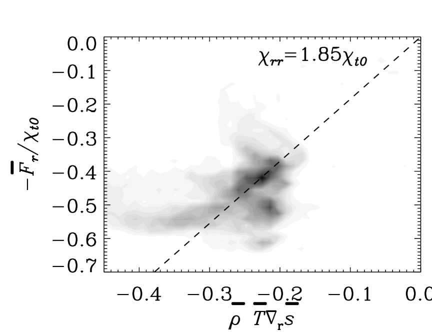
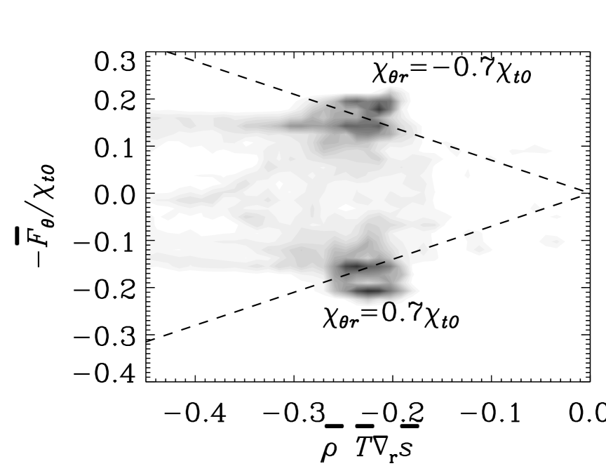
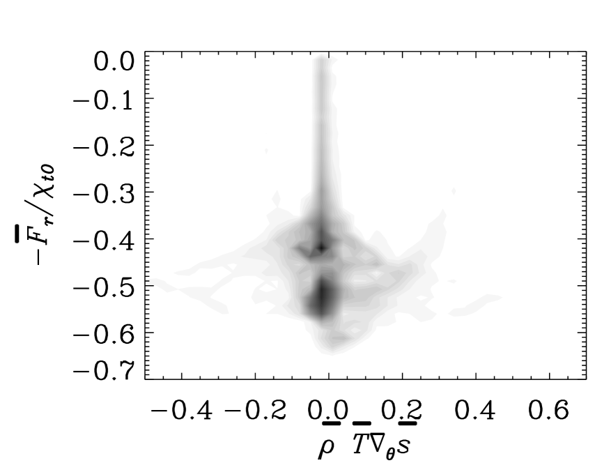
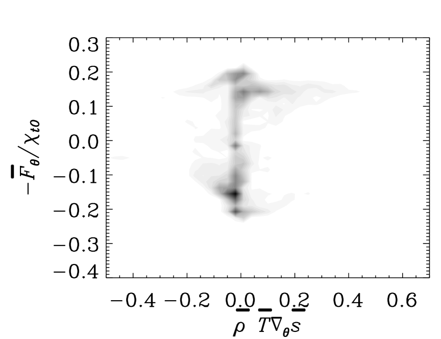
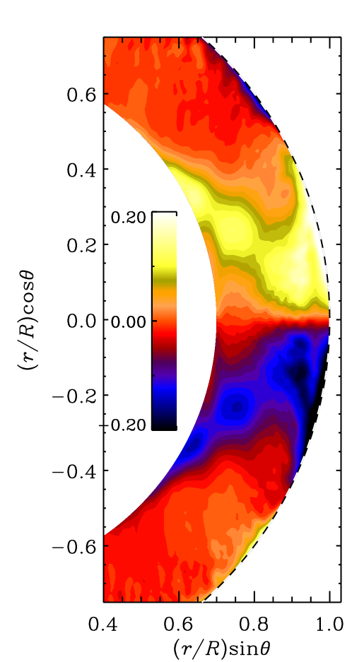
In reality, we cannot neglect the second term proportional to , even though this gradient is about 10 times smaller than in our simulations. To test the accuracy of Equations (23) and (24), we compute two-dimensional histograms of latitudinal and radial heat fluxes versus latitudinal and radial entropy gradients; see Figure 8. The determined values of the turbulent heat diffusivities of Figure 7 are consistent with those results. However, a clear linear trend is not visible, except for a narrow range in the case of . In the first panel, the line with fits the maximum of the correlation well. Indeed, looking at the left panel of Figure 7, is compatible with this. A similar behavior can be seen in the top-right panel of Figure 8. We see that the lines of fit well through the maxima of the data, but we cannot find any indication of a linear correlation, as suggested by Equations (23) and (24). The last two panels support our assumption that the latitudinal entropy gradient can be neglected when calculating the turbulent heat diffusivity. The main conclusion of the two-dimensional histogram is that the correlation suggested by Equation (23) and (24) is at best only true for the radial gradient of , but not for the latitudinal one. The ratio of the convective flux and the entropy gradient is dominated by the ratio of two points rather than a correlation. Although the latitudinal entropy gradient is only 10 times smaller than the radial one, we cannot find a linear correlation. This is surprising, given that these mean field relations have been used successfully to model the differential rotation profile as well as the turbulent heat transport of the Sun—in good agreement with observations (see, e.g., Kitchatinov & Rüdiger, 1995). In fact, as shown in the mean-field calculations of Brandenburg et al. (1992), the term tends to balance the first term so as to reduce the latitudinal heat flux and thus produce a latitudinal entropy gradient and a baroclinic term as we see it.
To investigate the baroclinic term and the turbulent heat diffusivities as well as their influence on the differential rotation in more detail, we compare the present runs, where we include a coronal envelope, with runs without a coronal envelope. The runs without a coronal envelope are taken from Käpylä et al. (2012) and Käpylä et al. (2013). Thus, we compare Figures 5 and 7 for Run A with the corresponding ones for Run C1 of Käpylä et al. (2013), which is the same as Run B4m of Käpylä et al. (2012); see Figures 9 and 10. As in Run A above, the baroclinic term of Run C1 balances the advection term. However, the values are four times larger and the shape shows a clear radial variation. The baroclinic term is largest near the surface, whereas in Figure 5 of Run A, the term is stronger near the bottom of the convection zone. In Run C1, on the other hand, the terms are small near the bottom and close to the equator. The component of the turbulent heat diffusivity tensor (Figure 10) looks quite different from Run A; compare with Figure 7. The radial heat conductivity is about two times smaller than in the runs with a corona. The mean radial entropy gradient has a positive sign at latitude, and extends from the bottom to the middle of the convection zone. How these two behaviors can change the solar-like rotation to a more cylindrical rotation is unclear. Stratification may be important, because in Run C1 without a corona the density contrast is , which is slightly higher than in the four runs of this work.
3.3. Meridional Circulation
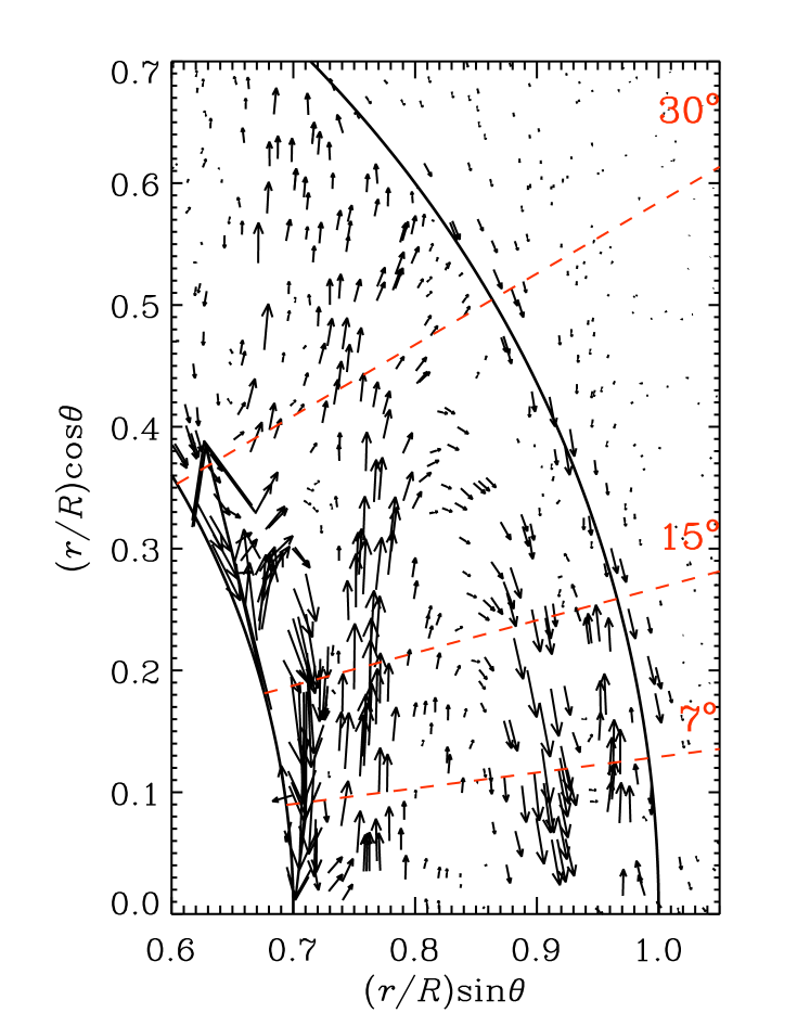
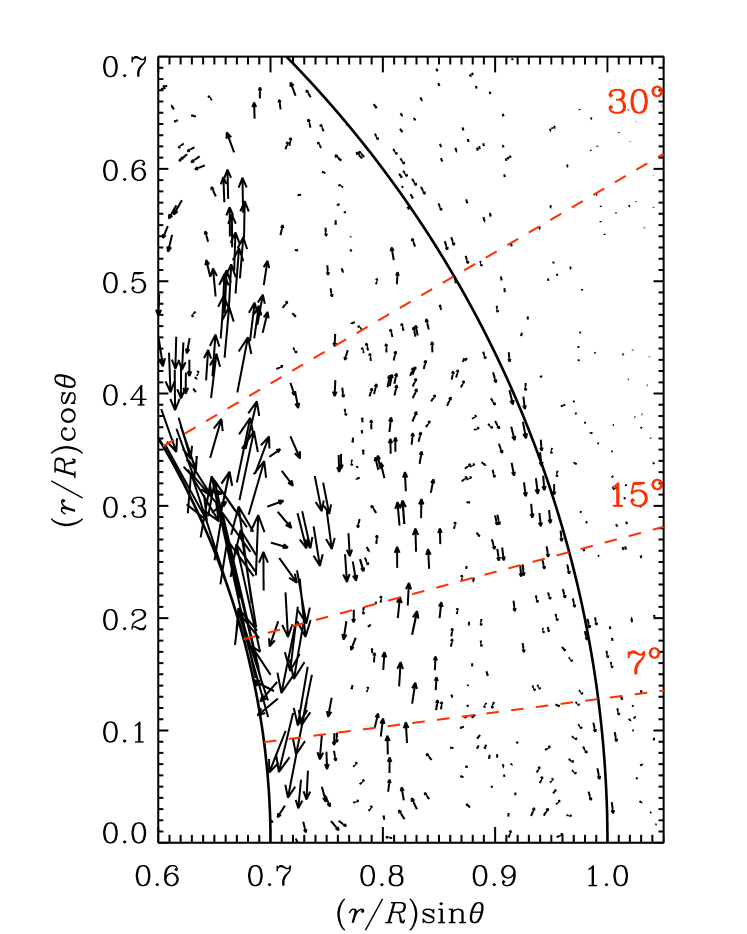
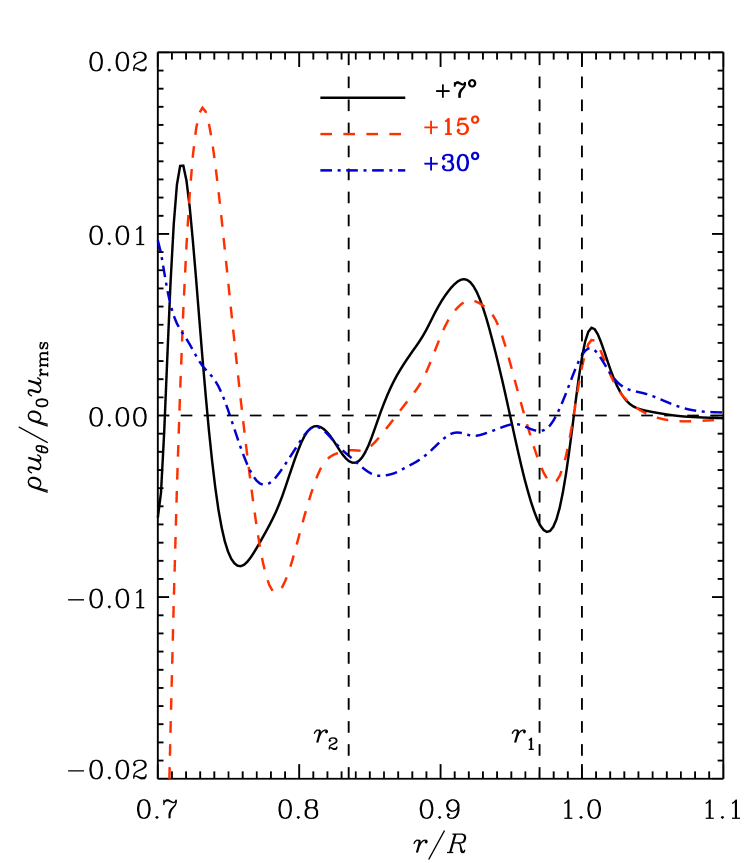
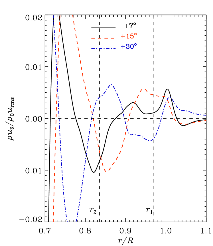
Another important result is the multi-cellular meridional circulation in the convection zone with a poleward (solar-like) flow near the surface. In Figure 11, we plot the meridional circulation in terms of the mass flux as vectors of and as radial cuts of through colatitudes = 60∘, = 75∘, and = 83∘, corresponding to latitudes of , , and . Note here that in the northern (southern) hemisphere a negative means a poleward (equatorward) flow, and a positive one equatorward (poleward) flow. Runs A, Ab, and Ac show significant solar-like surface profiles of meridional circulation, while Run B shows a different pattern. Looking at Run A, in the northern hemisphere at lower latitudes () just below the surface (), the meridional circulation is poleward with . Above the surface there is a return flow in the equatorward direction. This return flow peaks above the surface with a similar flux. The turning point is just below the surface, at around . The location of this turning point is consistent with the location where the entropy gradient changes from negative to positive, i.e., from convectively unstable to convectively stable; see Figure 1. If we were to redefine the surface of the simulated star to this radius, we would obtain a solar-like meridional circulation, where the circulation is poleward at the surface. The velocity near the surface is . To compare this with the meridional circulation at the surface of the Sun, which is m s-1 (Zhao & Kosovichev, 2004), we calculate the corresponding value of from the convective flux, , with a typical density of near the surface of the convection zone at (Stix, 2002). Our estimate of corresponding meridional circulation gives m s-1, which is consistent with the solar value. Similar estimates apply to the southern hemisphere, but the meridional circulation is a bit weaker here. This behavior can also be found in Runs Ab and Ac, where the flows are weaker and the turning points lie slightly deeper. Note that the strong return flow above the surface is a consequence of our particular setup, which has much weaker stratification than the Sun; see Figure 1. Higher stratification should lead to a much weaker return flow in this location. In Run B, a poleward flow develops in the northern hemisphere only close to poles (). The meridional circulation has a latitudinal dependence. In Run A the return flow reaches higher velocities at lower latitudes (). The same is true for the poleward circulation below the solar surface. In Run B, we find the opposite and both the return flow and the meridional circulation increase with latitude.
From the bottom row of Figure 11, we can estimate the number of meridional circulation cells at low latitudes. We find that there are at least two cells in the convection zone. In Run A, there is one cell with poleward flow maxima around and minima around , where the mass flux closer to the surface is as large as that in the return flow deeper in the convection zone. A second cell is deeper down in the convection zone and has similar extent and flux. A similar two-cell meridional flow pattern has recently been reported by Zhao et al. (2013) from helioseismic inversions of Solar Dynamics Observatory/Helioseismic and Magnetic Imager data. In Runs Ab and Ac, the pattern is different and the flux is weaker, but there are indications of a third cell. Note that the stratification leads to stronger mass fluxes over a smaller cross-sectional area deeper in the convection zone than near the surface, while the velocity is similar. In Run B, there are two strong cells of meridional circulation. The cells seem to be more cylindrical than latitudinal, which can also be seen in the phase shift of the pattern for different latitudes. Even deeper down in the convection zone, the meridional flow is much stronger than in Runs A, Ab, and Ac. This is consistent with results from models with anisotropic viscosity (or lowest order effect), which show a maximum of meridional circulation for Taylor numbers around (Köhler, 1970). Our Taylor number is above this value, so the circulation decreases with faster rotation, which is also in agreement with numerical simulations (Ballot et al., 2007; Brown et al., 2008; Augustson et al., 2012). We emphasize that this does not apply to the non-dimensional meridional circulation, normalized by viscosity, which does not show a maximum.
3.4. Mean Magnetic Field Evolution
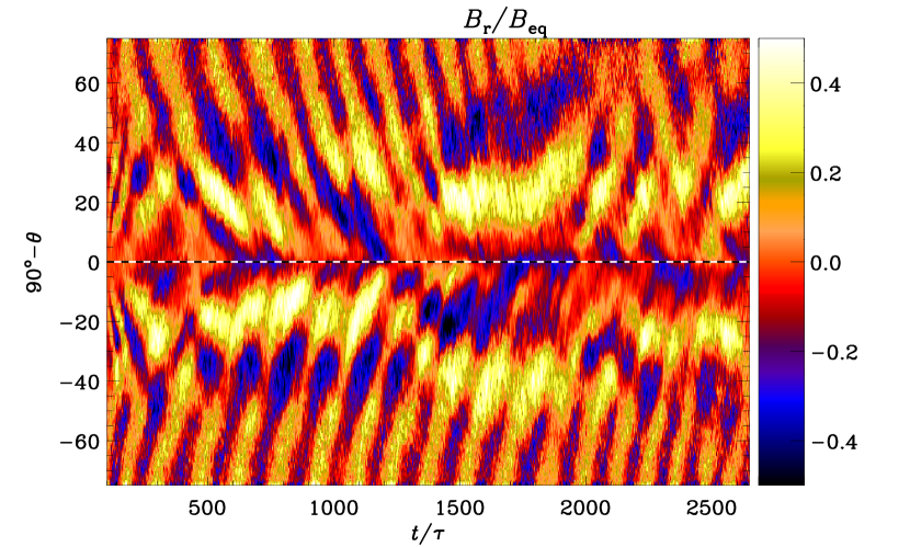
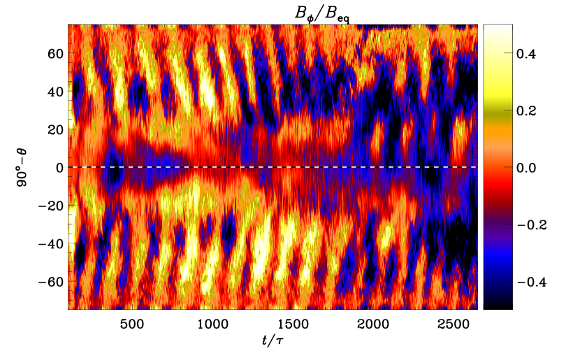
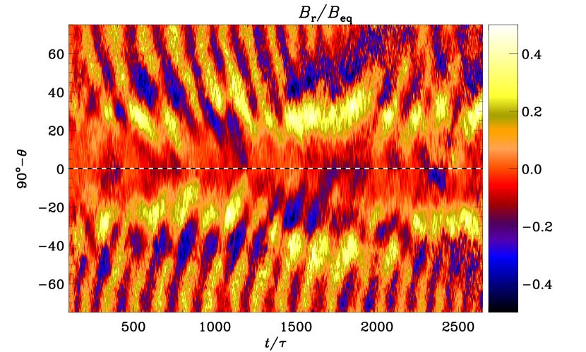
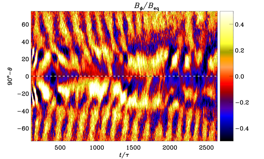
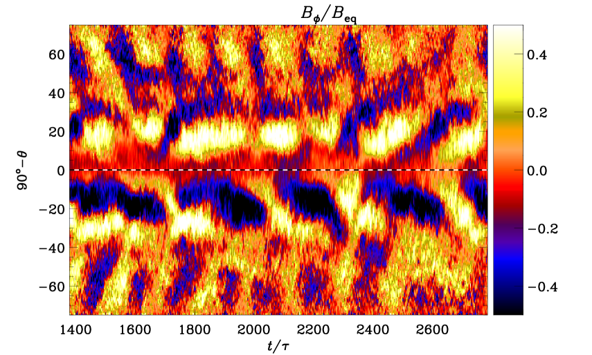
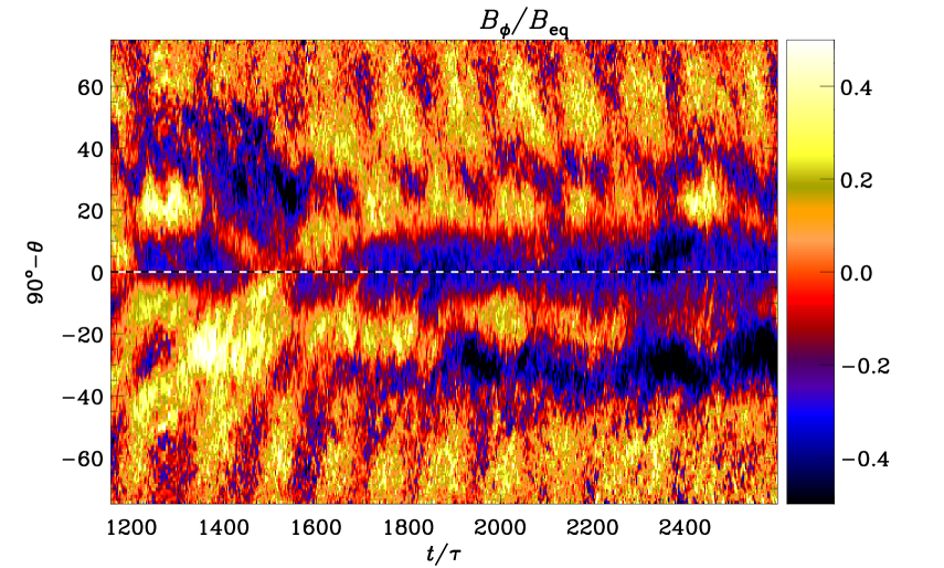
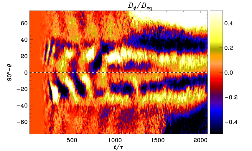
The turbulent helical motions generated by convective heat transport, together with differential rotation, produce a large-scale magnetic field inside the convection zone. It grows exponentially and shows an initial saturation after around for Run A; see Figure 2. Run B shows a more peculiar behavior: the field seems to have saturated at around , but it starts growing again at around and appears to saturate at . The latter growth is possibly related to a change of the oscillatory mode into a stationary one; see Figure 12 and the discussion below. The magnetic and fluid Reynolds numbers of Run B are higher than for the other cases, which should lead to a higher growth rate. However, the rotation rate measured by is around half that of Run A, which leads to a slower amplification of the field. At a later time, around , the field of Run B becomes comparable to or even stronger than that of Run A. The value of reaches around 0.5 of the equipartition field strength in Runs A, Ab, and Ac and 0.6 in Run B; see Table 1. In comparison, is around 20% lower because the field is mainly concentrated in the convection zone. The equatorward migration pattern is visible in three of the four runs at high latitudes. In Run A, the pattern seems to transform into a slow poleward migration at lower latitudes, but the equatorward migration pattern re-appears at . We suggest that the equatorward migrating dynamo mode is dominant after , while being overcome by other modes between and .
Comparing our results with those of Käpylä et al. (2012) without a corona but an otherwise comparable setup, the magnetic field in the current simulations is slightly weaker. In Figure 2 of Käpylä et al. (2012), the mean toroidal magnetic field strength is close to super-equipartition (), whereas in Figure 12 the mean magnetic field strength is roughly . Additionally, the growth rate of the dynamo is greater than in the models without corona, where it takes up to five times longer to reach dynamically important field strengths. This is not surprising because the dynamo in the two-layer model is less restricted and has more freedom for different dynamo modes to be excited. There is no restriction due to the magnetic boundary at the surface, which is open in our simulations, but restricted to vertical fields in the convection zone simulations of Käpylä et al. (2012). This could explain the fast growth in the beginning, but not the decreased saturation level. On the other hand, the runs in this work and the runs of Käpylä et al. (2012, 2013) also show differences in other parameters, such as stratification, rotation rate, and Reynolds numbers, so a direct comparison might not be possible.
Recently, other authors also have reported magnetic cycles. In the works by Brown et al. (2011) and Nelson et al. (2013), using anelastic LES, the authors were able to produce an oscillatory field, but without a clear pattern and no equatorward migration. In the simulations by Ghizaru et al. (2010) and Racine et al. (2011), who used an implicit method, the mean magnetic field shows a clear oscillatory behavior, but only a weak tendency for equatorward migration; see Figure 4 of Ghizaru et al. (2010) and Figure 8 of Racine et al. (2011). There is evidence that oscillatory solutions are favored when the density stratification is strong (Gastine et al., 2012), but such dynamos might well be of the type (Mitra et al., 2010; Schrinner et al., 2011), while strong shear favors poleward migration (Schrinner et al., 2012). At the moment, only the work by Käpylä et al. (2012, 2013) and the present work show clear evidence of equatorward migration.
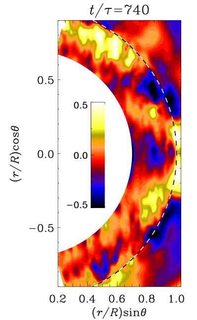
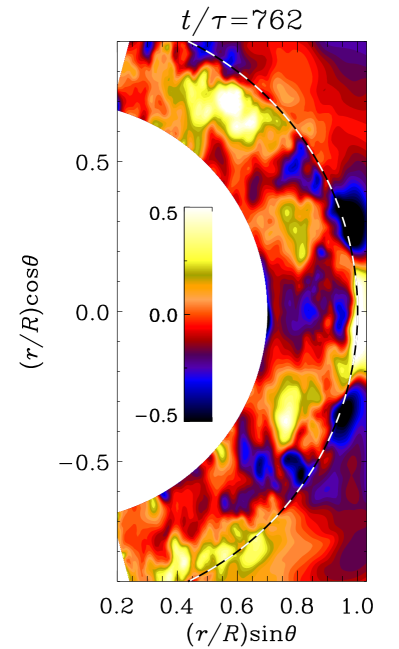
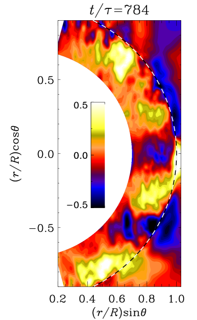
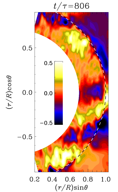
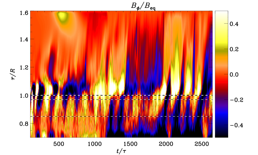
Looking just at in the convection zone or at in the whole domain in Figure 2, we find evidence of cyclical behavior of the field for Runs A, Ab, and Ac. The cycle period is . In Run B, there is no clear evidence of cyclical behavior. Investigating the different components of the mean magnetic field we find signs of oscillatory behavior for all runs, except that Run B shows oscillations only at early times. In Figure 12, we plot the azimuthal mean magnetic field over time and latitude at for Runs A, Ab, Ac, and B, while in Figure 13 we show at and the radial mean field at and for Run A. The structure of the magnetic field changes as the dynamo evolves from the kinematic regime, where the magnetic field is weak and does not significantly influence the flow. In Run A, the azimuthal and radial mean fields migrate poleward close to the equator in the kinematic regime. The cycle period is short, just around . In Run B, we find a similar behavior. The fast poleward migration happens at low latitudes () for both runs. We recall that in Run A, after a short time (), the field is strong enough to backreact on the flow. At that time, two things happen simultaneously: an oscillating mean magnetic field starts to migrate equatorward at higher latitudes and the fast poleward migration becomes slower. The period of the equatorward oscillation is longer and is between and for the rest of the run. This period is consistent with those obtained from the time series. The poleward migration near the equator slows down until it finally turns into an equatorward migration aligned with the migration at higher latitudes (). Thus, we have equatorward migration of the mean radial and azimuthal fields at all latitudes until around and again after ; see Figure 13. During this interval, the dynamo mode changes and, consequently, its latitudinal migration pattern changes. The equatorward migrating and oscillating field near the poles show a stable pattern during the whole simulation, but near the equator the field changes with time. In the northern hemisphere there is a transient poleward migration, which is in phase with the equatorward migration near the poles. In the southern hemisphere the equatorward migration is still dominant, but a stationary mode is superimposed near the equator. After , the equatorward migration returns and penetrates again to lower latitudes.
The migration patterns are not just features appearing close to the surface, but they penetrate the entire convection zone until the bottom, as seen in Figure 13. This makes it implausible that meridional circulation is the main driver of this migration. As discussed in Section 3.1, the meridional circulation shows strong variability in radius and has at least two cells.
Runs Ab and Ac have been restarted from a snapshot of Run A after and , respectively. In Run Ab we decrease the magnetic Prandtl number, while in Run Ac we increase it; see Table 1. This was done to investigate the influence of the magnetic Reynolds number on the equatorward migration. As seen from Figure 12 the pattern of the mean magnetic field is not strongly affected by this change. There is clear equatorward migration near the poles and some indication of poleward migration at low latitudes. It seems that Run Ac, with a higher magnetic Reynolds number, shows a clearer equatorward migration pattern. However, some stationary fields are superimposed on the field near the equator. In Run Ab, the field tends to migrate poleward near the equator and equatorward near the poles. In any case, a higher magnetic Reynolds number (keeping the other parameters the same) seems to support equatorward migration. This is promising because it goes in the right direction toward explaining the Sun, although the differences in Reynolds numbers are not large enough to draw strong conclusions.
In Run B, where the fluid and magnetic Reynolds numbers are higher and the rotation is slower than in Run A, the structure of the mean field evolution shows some differences. In the kinematic regime, the field is similar to that of Run A in which it migrates poleward at lower latitudes. Also, as the field gets stronger, it begins to migrate from higher latitudes toward the equator and the low-latitude fast poleward branch becomes slower. The main difference from Run A is that the poleward migration does not turn into equatorward migration near the equator. In Runs A, Ab, and Ac, the field strengths have no clear latitudinal dependence. In contrast, in Run B the field strength near the poles is around half the strength near the equator. Only during late times does the high-latitude branch increase in strength. In Runs A and Ac, the radial and azimuthal components have approximately the same strength, whereas in Run B, the radial mean magnetic field seems to be weaker by a factor of two. Also, Run B shows no clear radial dependence in the structure of the mean field. The period of the equatorward migrating field is , which is a bit longer than in Run A. The poleward migration near the equator has an irregular oscillation and is usually not in phase with the equatorward migration near the poles. At , the dynamo mode changes significantly. Not only does the magnetic field start to grow (see Figure 2), but the magnetic field also changes from an oscillatory pattern to a stationary one, or at least an oscillatory one with a much longer period; see Figure 12. In particular, in the northern hemisphere, the mean azimuthal field shows a strong increase in strength. The field pattern now consists of a strong time-independent component with a latitudinal dependence. Near the surface (at ; see Section 2) the field seems to migrate slowly toward the equator, but it is not possible to identify a migrating pattern in the present run.
If one translates the cycle period of the equatorward migration to solar values using a turnover time of 1 month, we obtain a cycle period of 12 and 16 yr for Runs A and B, respectively. This would be a typical value in the middle of the convection zone. However, if one uses the Coriolis numbers of our runs (see Table 1), then would be 0.7 months, which would lead to 9 yr and 12 yr for Runs A and B, respectively. The regular magnetic cycles in the work of Ghizaru et al. (2010) and Racine et al. (2011) have a somewhat longer period of 60 years. Nelson et al. (2013) and Brown et al. (2011) were only able to generate highly irregular cycles, with no clear reversal in both hemispheres. They therefore found a large range of cycle periods, which span from 1 yr to around 60 yr.
To investigate the equatorward migration, we plot the mean azimuthal magnetic field for eight different times for Run A, resolving one cycle; see Figure 14. The field penetrates the entire convection zone and has up to four regions with different polarities in one hemisphere. These polarities are migrating toward the equator. In the northern hemisphere at around latitude, there is a magnetic field concentration with positive polarity. After – (panel 5), we find a negative magnetic field concentration at the same location, and again after (panel 8) the same polarity as in the beginning of the cycle appears. One can see a clear cyclical equatorward migration of the field, but it is irregular. The two hemispheres do not show the same magnetic field strength and it seems that, from time to time, there is only one dominant polarity in one hemisphere, while in the other there are three. Note also the strong negative magnetic fields near and above the surface, which also seem to show cyclical behavior.
It is still unclear why the equatorward migration takes place, so we can only speculate about it. There are several candidate explanations. One is the meridional circulation, which shows a solar-like pattern in Runs A, Ab, and Ac. But, as shown in Figure 13, the equatorward migration is present throughout the bulk of the convective zone, while the meridional circulation becomes more incoherent with depth. The incoherence is a manifestation of the multi-cellular structure of the meridional circulation. The shape and number of cells are similar to those obtained in recent simulations by Käpylä et al. (2012) and Nelson et al. (2013) and observations by Zhao et al. (2013). This is quite different from the single cell circulation postulated in flux transport dynamo models to drive equatorward migration (e.g., Choudhuri et al., 1995; Dikpati & Charbonneau, 1999; Kitchatinov & Olemskoy, 2012). We can therefore conclude that we find no evidence for magnetic field generation similar to the mechanism proposed by the flux transport dynamo models. A second candidate is the contribution of current helicity of small-scales in the magnetic tensor. However, preliminary studies suggest that the isotropic part does not seem to play an important role here (Warnecke et al., 2013a). This point is not fully conclusive, because we have not yet determined the full anisotropic contributions to the magnetic quenching term (see Brandenburg & Subramanian, 2007, for a detailed description and discussion). Finally, Käpylä et al. (2013) used the phase difference of the poloidal and toroidal magnetic fields to argue that an dynamo is responsible for the equatorward migration in their model. This might also be the case here, which is also indicated by the fact that the amplitude ratio of poloidal to toroidal field is near unity; see Figure 13.
The radial dependence of the mean azimuthal magnetic field (see the last panel of Figure 13) suggests that most of the contribution to the cyclical behavior comes from the surface layers. First of all, the field is strong near and above the surface where the density stratification is large, but also at the bottom of the convection zone, at least after saturation. The oscillation pattern seems to be predominantly a surface phenomenon with extension to the bulk rather than one rooted deep in the convection zone. The field at the bottom of the convection zone has constant polarity, while in the bulk and at the surface of the convection the oscillation is quite pronounced. For example, at , a negative magnetic field rises from the bottom and gets concentrated near the surface while, at the same time, a positive field seems to be formed close to the surface and emerges above the surface where it gets concentrated. This suggests that the strong density stratification, which is present only very close to the surface of the Sun, might be responsible for the oscillation and the equatorward migration of the solar magnetic field.
Further investigations measuring the turbulent transport coefficients in their full tensorial form are necessary to determine the reason for the equatorward migration. Measuring the components of by neglecting the contributions of the turbulent magnetic diffusivity as by Racine et al. (2011), can be misleading. A more sophisticated approach is to use the so-called test-field method (Schrinner et al., 2007; Brandenburg et al., 2010) adapted for spherical coordinates.
4. Conclusions
We have used a model that combines the turbulent convective dynamo with a coronal layer to reproduce properties of the Sun. We found a solar-like differential rotation with roughly radial contours of angular velocity at low latitudes. This is accompanied by a multi-cellular meridional circulation, which is manifested as a solar-like poleward flow near the surface. Additionally, the differential rotation profiles show a near-surface shear layer in all of the four simulations we perform. In one of the four simulations, there also exists a similar layer above the surface. We identify the self-consistently generated, non-zero latitudinal entropy gradient as the main cause of the spoke-like differential rotation.
The mean magnetic field shows a pattern of equatorward migration similar to Käpylä et al. (2012, 2013). This pattern is mostly visible at higher latitudes and only in two of the simulation at lower latitudes. However, at intermediate times of the simulation, the equatorward migration is only visible at high latitudes, while at lower latitudes poleward migration or stationary modes occur. In one of the simulations, the dynamo mode changed to a stationary one on all latitudes at later stages. The dynamo has a shorter excitation time than in the earlier work of Käpylä et al. (2012).
The present work leads to the conclusion that the inclusion of a coronal layer in convective dynamo simulations has an influence on the fluid and magnetic properties of the interior. In recent simulations, we were able to produce recurrent coronal ejections from the solar surface (Warnecke et al., 2012b) using a two layer approach. In earlier models of forced turbulence with a coronal layer (Warnecke & Brandenburg, 2010; Warnecke et al., 2011, 2012a), we also found ejection of magnetic helicity out of the dynamo region. These ejections can support and amplify the magnetic field due to significant magnetic helicity fluxes.
Here, we present evidence that even the fluid properties in the bulk of the convection zone might be influenced by the coronal layer. Spoke-like rotation profiles could not be obtained by earlier DNS of convective dynamos (Käpylä et al., 2012) without prescribing a latitudinal entropy gradient at the bottom of the convection zone (Miesch et al., 2006) or adding a stably stratified layer below the convection zone (Brun et al., 2011) in purely hydrodynamical LES. However, to have more convincing evidence in support of this, we need to perform a detailed parameter study using different coronal sizes and compare them with simulations without a corona.
Another extension of our work is the measurement of magnetic helicity fluxes through the surface and their dependence on the size of the corona. To investigate the mechanism of the equatorward migration, which is crucial for understanding the solar dynamo, one should measure the turbulent transport coefficients through approaches like the test-field method (Schrinner et al., 2007).
In further work, we plan to investigate the possibility of producing coronal ejections using the setup of these runs. In comparison with Warnecke et al. (2012b), we use here a corona with a much higher temperature and a lower plasma beta. It will be interesting to see how the coronal ejections are influenced by these changes.
References
- Augustson et al. (2012) Augustson, K. C., Brown, B. P., Brun, A. S., Miesch, M. S., & Toomre, J. 2012, ApJ, 756, 169
- Ballot et al. (2007) Ballot, J., Brun, A. S., & Turck-Chièze, S. 2007, ApJ, 669, 1190
- Blackman & Brandenburg (2003) Blackman, E. G., & Brandenburg, A. 2003, ApJ, 584, L99
- Brandenburg (2005) Brandenburg, A. 2005, ApJ, 625, 539
- Brandenburg et al. (2010) Brandenburg, A., Chatterjee, P., Del Sordo, F., Hubbard, A., Käpylä, P. J., & Rheinhardt, M. 2010, PhST, 142, 014028
- Brandenburg et al. (1992) Brandenburg, A., Moss, D., & Tuominen, I. 1992, A&A, 265, 328
- Brandenburg & Sandin (2004) Brandenburg, A., & Sandin, C. 2004, A&A, 427, 13
- Brandenburg & Subramanian (2005) Brandenburg, A., & Subramanian, K. 2005, Phys. Rep., 417, 1
- Brandenburg & Subramanian (2007) Brandenburg, A., & Subramanian, K. 2007, AN, 328, 507
- Brown et al. (2008) Brown, B. P., Browning, M. K., Brun, A. S., Miesch, M. S., & Toomre, J. 2008, ApJ, 689, 1354
- Brown et al. (2011) Brown, B. P., Miesch, M. S., Browning, M. K., Brun, A. S., & Toomre, J. 2011, ApJ, 731, 69
- Brun et al. (2004) Brun, A. S., Miesch, M. S., & Toomre, J. 2004, ApJ, 614, 1073
- Brun et al. (2011) Brun, A. S., Miesch, M. S., & Toomre, J. 2011, ApJ, 742, 79
- Choudhuri et al. (1995) Choudhuri, A. R., Schüssler, M., & Dikpati, M. 1995, A&A, 303, L29
- Dikpati & Charbonneau (1999) Dikpati, M., & Charbonneau, P. 1999, ApJ, 518, 508
- Gastine et al. (2012) Gastine, T., Duarte, L., & Wicht, J. 2012, A&A, 546, A19
- Ghizaru et al. (2010) Ghizaru, M., Charbonneau, P., & Smolarkiewicz, P. K. 2010, ApJ, 715, L133
- Gilman (1983) Gilman, P. A. 1983, ApJS, 53, 243
- Hubbard & Brandenburg (2012) Hubbard, A., & Brandenburg, A. 2012, ApJ, 748, 51
- Käpylä et al. (2010) Käpylä, P. J., Korpi, M. J., Brandenburg, A., Mitra, D., & Tavakol, R. 2010, AN, 331, 73
- Käpylä et al. (2006) Käpylä, P. J., Korpi, M. J., & Tuominen, I. 2006, AN, 327, 884
- Käpylä et al. (2011a) Käpylä, P. J., Mantere, M. J., & Brandenburg, A. 2011a, AN, 332, 883
- Käpylä et al. (2012) Käpylä, P. J., Mantere, M. J., & Brandenburg, A. 2012, ApJ, 755, L22
- Käpylä et al. (2013) Käpylä, P. J., Mantere, M. J., Cole, E., Warnecke, J., & Brandenburg, A. 2013, ApJ, 778, 41
- Käpylä et al. (2011b) Käpylä, P. J., Mantere, M. J., Guerrero, G., Brandenburg, A., & Chatterjee, P. 2011b, A&A, 531, A162
- Karak (2010) Karak, B. B. 2010, ApJ, 724, 1021
- Kitchatinov & Olemskoy (2012) Kitchatinov, L. L., & Olemskoy, S. V. 2012, Sol. Phys., 276, 3
- Kitchatinov & Rüdiger (1995) Kitchatinov, L. L., & Rüdiger, G. 1995, A&A, 299, 446
- Köhler (1970) Köhler, H. 1970, Sol. Phys., 13, 3
- Krause & Rädler (1980) Krause, F., & Rädler, K.-H. 1980, Mean-field Magnetohydrodynamics and Dynamo Theory (Oxford: Pergamon)
- Miesch et al. (2006) Miesch, M. S., Brun, A. S., & Toomre, J. 2006, ApJ, 641, 618
- Mitra et al. (2009) Mitra, D., Tavakol, R., Brandenburg, A., & Moss, D. 2009, ApJ, 697, 923
- Mitra et al. (2010) Mitra, D., Tavakol, R., Käpylä, P. J., & Brandenburg, A. 2010, ApJ, 719, L1
- Nelson et al. (2013) Nelson, N. J., Brown, B. P., Brun, A. S., Miesch, M. S., & Toomre, J. 2013, ApJ, 762, 73
- Racine et al. (2011) Racine, É., Charbonneau, P., Ghizaru, M., Bouchat, A., & Smolarkiewicz, P. K. 2011, ApJ, 735, 46
- Rempel (2005) Rempel, M. 2005, ApJ, 622, 1320
- Rüdiger (1980) Rüdiger, G. 1980, GApFD, 16, 239
- Rüdiger (1989) Rüdiger, G. 1989, Differential Rotation and Stellar Convection. Sun and Solar-type Stars (Berlin: Akademie)
- Schou et al. (1998) Schou, J., et al. 1998, ApJ, 505, 390
- Schrinner et al. (2011) Schrinner, M., Petitdemange, L., & Dormy, E. 2011, A&A, 530, A140
- Schrinner et al. (2012) Schrinner, M., Petitdemange, L., & Dormy, E. 2012, ApJ, 752, 121
- Schrinner et al. (2007) Schrinner, M., Rädler, K.-H., Schmitt, D., Rheinhardt, M., & Christensen, U. R. 2007, GApFD, 101, 81
- Spiegel & Weiss (1980) Spiegel, E. A., & Weiss, N. O. 1980, Nature, 287, 616
- Stix (2002) Stix, M. 2002, The Sun: An Introduction (Berlin: Springer)
- Warnecke & Brandenburg (2010) Warnecke, J., & Brandenburg, A. 2010, A&A, 523, A19
- Warnecke et al. (2011) Warnecke, J., Brandenburg, A., & Mitra, D. 2011, A&A, 534, A11
- Warnecke et al. (2012a) Warnecke, J., Brandenburg, A., & Mitra, D. 2012a, JSCSW, 2, A11
- Warnecke et al. (2012b) Warnecke, J., Käpylä, P. J., Mantere, M. J., & Brandenburg, A. 2012b, Sol. Phys., 280, 299
- Warnecke et al. (2013a) Warnecke, J., Käpylä, P. J., Mantere, M. J., & Brandenburg, A. 2013a, in IAU Symposium, Vol. 294, IAU Symposium, ed. A. G. Kosovichev, E. de Gouveia Dal Pino, & Y. Yan, 307–312
- Warnecke et al. (2013b) Warnecke, J., Losada, I. R., Brandenburg, A., Kleeorin, N., & Rogachevskii, I. 2013b, ApJ, 777, L37
- Weiss (1965) Weiss, N. O. 1965, Obs, 85, 37
- Zhao et al. (2013) Zhao, J., Bogart, R. S., Kosovichev, A. G., Duvall, T. L., & Hartlep, T. 2013, ApJ, 774, L29
- Zhao & Kosovichev (2004) Zhao, J., & Kosovichev, A. G. 2004, ApJ, 603, 776