Classification of missing values in spatial data using spin models

Abstract

A problem of current interest is the estimation of spatially distributed processes at locations where measurements are missing. Linear interpolation methods rely on the Gaussian assumption, which is often unrealistic in practice, or normalizing transformations, which are successful only for mild deviations from the Gaussian behavior. We propose to address the problem of missing values estimation on two-dimensional grids by means of spatial classification methods based on spin (Ising, Potts, clock) models. The “spin” variables provide an interval discretization of the process values, and the spatial correlations are captured in terms of interactions between the spins. The spins at the unmeasured locations are classified by means of the “energy matching” principle: the correlation energy of the entire grid (including prediction sites) is estimated from the sample-based correlations. We investigate the performance of the spin classifiers in terms of computational speed, misclassification rate, class histogram and spatial correlations reproduction using simulated realizations of spatial random fields, real rainfall data, and a digital test image. We also compare the spin-based methods with standard classifiers such as the $k$-nearest neighbor, the fuzzy $k$-nearest neighbor, and the Support Vector Machine. We find that the spin-based classifiers provide competitive choices.

I Introduction

To date there is a growing demand for various types of spatial data, including remote sensing images, such as thematic maps representing geographical variables, natural resources, land use, environmental indicators, or economic and demographic information. At the same time, new methods are needed for the efficient and reliable processing, analysis, and digital storage of this information. Common issues that arise in the processing phase include the heterogeneity of the data, i.e., the fact that they come from different sources (sensors) operating at different resolutions and often with different biases. In addition, the data coverage is often incomplete due to limited resources (material, human, or technical), equipment limitations (detection level, resolution), meteorological conditions (observations hindered by clouds) and sensor malfunctions.

In the following, we will assume that an observed spatially distributed process in two dimensions is a realization of a spatial random field (SRF) yagl87 . An SRF, $Z(\vec{r},\omega)$, where $\vec{r}=(x,y)\in\mathbb{R}^{2}$ is the location and $\omega$ is the state index, represents an ensemble of states (realizations), the spatial correlations of which are determined by a joint probability density function (p.d.f.). The state index will be suppressed in the following to keep the notation concise. In order to use standard tools for the analysis of space-time data, the observed process needs to be estimated at the missing value locations. The spatial estimation can be performed by means of established interpolation and classification techniques (atk99, ). However, considering the ever increasing size of spatial data, classical methods, e.g., kriging (wack03, ) and minimum curvature estimation min-curv , become impractical due to high computational complexity. Furthermore, the linear spatial interpolation methods assume a jointly Gaussian p.d.f., which is often not justified by data. In addition, the use of such methods typically requires a considerable degree of subjective input (dig07, ). The nonlinear indicator kriging (IK) method is based on a binary discretization of the data distribution with respect to an arbitrary number of thresholds journel83 . IK does not require the Gaussian assumption, but the predicted indicator values are not guaranteed to take $0$ or $1$ values, and may even lie outside the $[0,1]$ range.

Recent studies investigate applications of statistical physics concepts in various non-traditional fields, such as economy and finance man_stan99 ; bo_pot00 ; bouch00 , materials science kard95 ; wouts07 ; zhen06 , and biology gran92 . Most studies have focused on long-range correlations, while short-range correlations that can be used for spatial or temporal interpolation have received less attention. Nevertheless, within the Gibbs-Markov Random Field framework, the Potts and Ising models have been used in image analysis besa86 ; gimel99 ; kato06 ; zhao07 ; tana95 . The Potts model in the superparamagnetic regime has also been applied to the data clustering problem blatt96 and a Potts-model-based non-parametric approach employing simulated annealing to the oil reservoir characterization farm92 .

Let us consider the Gibbs probability density function $f_{\rm Z}={e^{-H[Z(\vec{r})]/k_{B}T}}/{\mathcal{Z}},$ where $H[Z(\vec{r})]$ is an interaction functional that involves spatial operators acting on the field $Z(\vec{r})$, $k_{B}$ is the Boltzmann’s constant, $T$ is the temperature (we can set $k_{B}\,T=1$ without loss of generality), and ${\mathcal{Z}}$ is the partition function. Assume that $H[Z(\vec{r})]$ measures the “spatial disorder energy” of the observed process. Hence, $H[Z(\vec{r})]$ is minimized for a uniform state and increases proportionally to the fluctuations of $Z$, as prescribed by the interactions embodied in $H[Z(\vec{r})]$. The family of Spartan Spatial Random Fields (SSRF) is based on the idea that the spatial correlations can be adequately determined from a general $H[Z(\vec{r})]$ dth03 with local interactions. However, the SSRF models are still based on the restrictive Gaussian assumption.

Mild deviations from Gaussian dependence including lognormal dependence can be treated by means of normalizing non-linear transformations. Alternatively, one can try to incorporate the non-Gaussian terms directly into the statistical model. However, it is not clear what type of interactions in $H[Z(\vec{r})]$ can generate the non-Gaussian behavior encountered in different data sets. Even if such interactions could be defined, calculation of the statistical moments would entail numerical integrations. The purpose of this study is to present non-parametric and computationally efficient methods that do not assume a specific form for the p.d.f. of the observed process. The main idea is to employ interaction models either of the form $H[S^{q}(Z(\vec{r}))],$ where $S^{q}(Z(\vec{r}))$ is a binary discretization of the continuous SRF $Z(\vec{r})$ and $q$ is a level index (i.e., Ising model), or of the form $H[S(Z(\vec{r}))]$, where $S(Z(\vec{r}))$ is a multilevel discretization of $Z$ (i.e., Potts and clock models). For the interaction functional we use spin (Ising, Potts and clock) Hamiltonians. Parameter estimation in such systems is typically based on computationally intensive Monte Carlo simulations or potentially inaccurate approximation methods. To overcome these problems, we develop a non-parametric, Monte Carlo based approach, which benefits from an informative assignment of the initial spin states.

The rest of the paper is organized as follows. In Section II, we discuss the problem of spatial classification/prediction and review some established machine learning classification algorithms. In Section III we develop our spatial classification approach based on spin models. Section IV investigates the application of the proposed models to synthetic realizations of spatial random fields. Section V focuses on the application of the spin-based classifiers on real data. Finally, in Section VI we summarize our results and discuss issues for future research.

II Spatial prediction and classification

We consider observations distributed on rectangular grids $\tilde{G}$ of size $N_{G}=L_{x}\times L_{y}$, where $L_{x}$ and $L_{y}$ are respectively the horizontal and vertical dimensions of the rectangle (in terms of the unit length). We denote the set of sampling points by $G_{s}=\{\vec{r}_{i}\}$, where $\vec{r}_{i}=(x_{i},y_{i})\in{\mathbb{R}}^{2},$ $i=1,\ldots,N$ are points scattered on the grid and $N=(1-p)\,N_{G}<N_{G}$. Let $z_{i}$ be the observation at $\vec{r}_{i}$ obtained from a joint p.d.f. $f_{\rm Z}(z_{1},\ldots,z_{N_{G}})$. The set $Z_{s}=\{z_{i}\in{\mathbb{R}}\}$ represents the sample of the process. Let $G_{p}=\{\vec{r}_{p}\},$ $p=1,\ldots,P=p\,N_{G}$, be the prediction set so that $\tilde{G}=G_{s}\cup G_{p}$. In the following we discretize the continuous distribution of $Z$ using a number of classes (intervals), ${\mathcal{C}}_{q},\,q=1,\ldots,N_{c}$. The classes are defined with respect to threshold levels $t_{k},\,k=1,\ldots,N_{c}+1$. If $Z_{\rm min}=\min(z_{1},\ldots,z_{N}),$ and $Z_{\rm max}=\max(z_{1},\ldots,z_{N})$ denote respectively the minimum and maximum values of the data and $\epsilon$ is an infinitesimal positive number, then $t_{1}=Z_{\rm min}-\epsilon$ and $t_{N_{c}+1}=Z_{\rm max}$. The remaining thresholds are defined by means of $t_{q}=(q-1)\,\left(Z_{\max}-Z_{\min}\right)/N_{c}+Z_{\min}$, for $q=2,\ldots,N_{c}.$ Each class ${\mathcal{C}}_{q}$ corresponds to an interval ${\mathcal{C}}_{q}=(t_{q},t_{q+1}]$ for $q=1,\ldots,N_{c}$. The class indicator field $I_{Z}(\vec{r})$ is defined so that $I_{Z}(\vec{r})=q$ if $z(\vec{r})\in{\mathcal{C}}_{q},$ for $q=1,\ldots,N_{c}$, i.e.,

$$I_{Z}(\vec{r}_{i})=\sum_{q=1}^{N_{c}}q\,\left[\theta\left(z_{i}-t_{q}\right)-\theta\left(z_{i}-t_{q+1}\right)\right],\quad\forall i=1,\ldots,N,$$ (1)

where $\theta(x)=1$ for $x>0$ and $\theta(x)=0$ for $x\leq 0$ is the unit step function. Prediction of the field values $Z\{G_{p}\}$ is then mapped onto a classification problem, i.e., the estimation of $\hat{I}_{Z}\{G_{p}\}$. For environmental monitoring and risk management applications useful answers can be obtained in terms of a small number of levels (e.g., eight). For the analysis of gray-scale digital images $256$ levels are typically required. As the number of levels tends to infinity, the discretized interval representation tends to the continuum, and spatial classification tends to spatial interpolation.

To test the performance of the spin-based classification methods, we use synthetic Gaussian (normal) and lognormal random field realizations on $L\times L$ grids (where $L=50,100,200$), continuous precipitation data sampled on a $50\times 50$ grid, and a digital $512\times 512$ image of $256$ gray-scale values. Each data set is randomly and exhaustively partitioned into sampling and prediction sets. We use the points in the prediction set for validation, i.e., to compare the true value of the process with the classifier predictions. Next, we briefly review two non-parametric, machine learning classification algorithms, which we use as benchmarks for the performance of the spin models.

II.1 $k$-nearest neighbor models

The $k$-nearest neighbor (KNN) model is probably the simplest of all machine learning algorithms dasa91 . The classified value is assigned to the most populated class among the $k$ nearest neighbors of the classification point. The distance metric used is typically Euclidean, and the neighbors are selected from the points in $G_{s}$. The optimal choice of the parameter $k$ is data dependent. Various heuristic techniques can be used to determine the optimal $k$, e.g. cross-validation. However, the method is sensitive to noise or the presence of irrelevant features at the scales of interest. Nevertheless, KNN typically outperforms many other flexible nonlinear methods, particularly when the number of explanatory variables is high cher96 . It is also easy to implement, and its classification error is asymptotically optimal.

An extension of KNN is the method of fuzzy $k$-nearest neighbor (FKNN) classification kell85 . In FKNN, the sampling points $\vec{r}_{j}$ are first assigned a membership to each class ${\mathcal{C}}_{q},\,q=1,\ldots,N_{c}$ by means of the function $u_{q}(\vec{r}_{j}).$ Then, each prediction point $\vec{r}_{p}$ is also assigned class membership according to the function $u_{q}(\vec{r}_{p})=\big{[}\sum_{j=1}^{k}u_{q}(\vec{r}_{j})\,||\vec{r}_{p}-\vec{r}_{j}||^{2/(1-m)}\big{]}/\big{(}\sum_{j=1}^{k}||\vec{r}_{p}-\vec{r}_{j}||^{2/(1-m)}\big{)}$, for $q=1,\ldots,N_{c}$. The parameter $m$ controls the influence of distant samples. Following kell85 we set $m=2$. The prediction points are classified according to the maxima of the membership functions. The FKNN classifier statistically reduces the effect of noisy samples and produces overall more accurate results than the classical KNN classifier. To eliminate the impact of an arbitrary $k$, we repeat the classification for $k=1,\ldots,k_{\max}$, to determine a $k_{\rm opt}$ that minimizes the misclassification rate. This adaptive approach guarantees that the lowest misclassification rates achievable by the KNN and the FKNN algorithms (based on the Euclidean distance metric) are used in the comparisons.

II.2 Support vector machines

The support vector machines (SVM) classifier is a supervised learning algorithm vapnik63 ; aizerman64 ; vapn98 which in several comparative studies outperformed other methods herm99 ; shari03 ; mull97 . The original SVM algorithm vapnik63 is a linear classifier that segregates data into two classes using maximum-margin hyperplanes. The SVM algorithm has been extended to multi-class and non-linear problems using the kernel function trick aizerman64 , by means of which nonlinear dependence is linearized in a higher-dimensional “feature” Hilbert space. The SVM method is robust and can handle high-dimensional data. However, it is computationally intensive, especially for large $N$ and $N_{c}$, because it requires the careful tuning of hyperparameters for each binary classifier followed by the solution of a quadratic problem with $N$ variables.

We solve the $N_{c}>2$ classification problem by means of $N_{c}$ binary classifiers operating in one-to-rest fashion e.g. hsulin02 . We use the software GeoSVM, which implements an adaptation of SVM for spatial data classification kane04 . The code is run with radial basis function (RBF) kernels and involves two tunable hyperparameters: the kernel bandwidth $\sigma_{k}$ and the regularization parameter $C$; the latter controls the trade-off between the machine complexity and the number of linearly non-separable points. The hyperparameters are tuned to minimize the misclassification rate. Due to the high computational cost of tuning and training the SVM, it is only applied to the rainfall data.

III Spatial classification based on spin models

Below we propose three non-parametric classifiers that use spin model Hamiltonians from statistical physics. In the following, the spins correspond to discretized levels of the continuous variable $Z$ and should not be confused with magnetic moments. The main idea is that the spatial correlations of $Z$ can be captured by the spin interactions. By focusing on the spins it is not necessary to assume a specific form of the joint p.d.f. $f_{Z}.$ The non-parametric form of the classifiers derives from the fact that the state of the spin systems is constrained by the sample data instead of the interaction couplings $J$ and the temperature $T$. This is convenient since $J$ and $T$ are unknown a priori, their estimation from the data can be computationally intensive due to the intractability of the partition function, and their uniqueness is not guaranteed for any given sample. To classify the values at the prediction points we use the heuristic principle of energy matching: we calculate the correlation energy of the sample normalized by the number of interacting spin pairs, and then determine the spin values at the prediction sites so that the normalized energy for the entire grid matches the respective sample value. Herein we focus on nearest neighbor correlations, but this constraint can be relaxed.

The idea of correlation energy matching has been applied in the statistical reconstruction of digitized (binary) random media from limited morphological information yeong98a ; yeong98b . The classifiers proposed here employ both local (sample values) and global (statistical) information. In particular, this is achieved by performing conditional simulations, in which the sample values are respected locally and the correlation energy globally. This means that while the interactions are translation invariant, the state of the system is not necessarily stationary (statistically homogeneous). The correlation energy matching presupposes that the nearest-neighbor separations in the sample capture the target scale of the prediction set. For example, assume that a sample is drawn from a square grid with step $\alpha$ by removing $50\%$ of the points. The energy matching will be more effective if the points are removed at random than if every second point is removed. In the first case, it is likely that contiguous groups of points will be removed, leaving pairs of neighbors separated by $\alpha$, while in the second case the minimum separation between the sampling points will be $2\alpha.$

The Ising model mccoy73 was introduced to describe the energy states of magnetic materials and later found many applications, e.g., as a model of neuron activity in the brain. It involves binary variables $s_{i}$ (spins), which can take the values $1$ or $-1$. In the absence of an external filed, the energy of the spin system can be expressed by the Hamiltonian $H_{I}=-\sum_{i,j}J_{ij}\,s_{i}\,s_{j}$. The coupling parameter $J_{ij}$ controls the type ($J_{ij}>0$ for ferromagnetic and $J_{ij}<0$ for antiferromagnetic coupling) and strength of the pairwise interactions. The model is usually defined on a regular grid, the interactions are considered uniform, and their range is limited to nearest neighbors. Generalizations to irregular grids and longer-range interactions are also possible. The Ising model has been solved in one dimension and in $d=2$ without external field. The Potts model is a generalization of the Ising model wu82 . Each spin variable is assigned an integer value $s_{i}\in\{1,\ldots,N_{c}\}$, where $N_{c}$ represents the total number of states. The Hamiltonian of the Potts model is given by $H_{P}=-\sum_{i,j}J_{ij}\delta_{(s_{i},s_{j})},$ where $\delta$ is the Kronecker symbol. Hence, nonzero contributions to the energy only come from spins in the same state. For $N_{c}=2$ the Potts model is equivalent to the 2D Ising model. The clock model, also known as the vector Potts model, assumes that the spins take one of $N_{c}$ possible values, which are distributed uniformly around a circle. The clock Hamiltonian is given by $H_{C}=-\sum_{i,j}J_{ij}\cos\Big{[}\frac{2\pi}{N_{c}}(s_{i}-s_{j})\Big{]}.$ In contrast with the Potts model, in the clock model interactions between spins in different states contribute to the interaction energy. The XY model is obtained from the clock model at the continuum limit $N_{c}\rightarrow\infty$. The presence of an external field $h_{i}$ implies an additional term $-\sum_{i}h_{i}s_{i}$ in the Hamiltonian. This term breaks the symmetry of the energy under spin reversals, and controls the total magnetization of the spins.

In typical applications of the spin models the parameters $J_{ij}$ and $h_{i}$ are assumed to be known, and the problem of interest is the estimation of various correlation functions. In the case of spatial data analysis, the parameters are not known a priori. Hence, prediction of the spins at unmeasured locations requires us to determine the model parameters from the available spin configuration (sample). The standard procedure for solving such an inverse problem is to infer the parameters by means of the maximum likelihood estimation (MLE) method. Then, the spin values at unsampled locations can be predicted by maximizing the p.d.f. $f_{Z}$ (equivalently, by minimizing $H$) under the data constraints. However, the analytical intractability of ${\mathcal{Z}}$ hampers the application of MLE. Possible ways of circumventing this problem, such as the maximum pseudo-likelihood besa75 approach or Markov chain Monte Carlo techniques chen97 can be inaccurate or prohibitively slow.

To bypass the problems mentioned above, we propose a non-parametric approach. For lattice data we assume that $J_{ij}=J$ for nearest neighbors and $J_{ij}=0$ otherwise. In addition, we consider a zero external field. Nevertheless, as shown by the simulation results below, the marginal class distributions of the data are recovered based on the interaction energy of the discretized levels and a judicious choice of the initial states (for each class). The use of different spin models in the study allows us to investigate the impact on the misclassification rate and prediction errors of different classification strategies (sequential vs. simultaneous), different couplings (intra-level vs. inter-level interactions), as well as the transition to the continuum case (XY model).

III.1 Classification based on the Ising Model

Here we present a spatial classification approach based on the Ising spin model with nearest neighbor correlations (INNC). The main idea is to use a sequential discretization scheme to estimate the class indicator field $\hat{I}_{Z}(G_{p}).$ In this scheme the sample $G_{s}^{q}$ and prediction, $G_{p}^{q}$ grids are progressively updated for increasing class index $q$. For the lowest class $G_{s}^{1}=G_{s},\,G_{p}^{1}=G_{p},$ where $G_{s}$ and $G_{p}$ are the sampling and prediction grids respectively. Let $N_{q}$ denote the number of sites on $G_{s}^{q}$ that have fixed class indicator values at level $q$; at the first level $N_{1}=N$ and $N_{q+1}\geq N_{q}$ for $q=1,\ldots,N_{c}-1$ since the sample at level $q+1$ is augmented by the points that are assigned fixed indicator values at level $q$. Let $S^{q}_{s}=\{s^{q}_{i_{q}}\}$, $q=1,\ldots,N_{c};$ $i_{q}=1,\ldots,N_{q}$ be the set that includes all the sample spin values with respect to level $q$, and $\tilde{S}^{q}=S^{q}_{s}\cup S^{q}_{p}$ denote all the spin values on $\tilde{G}$. The Ising model is used to represent interactions between the spins $\tilde{S}^{q}$.

At each level, the discretization is binary with respect to the upper threshold; i.e., $s^{q}_{i}=-1$ if $z_{i}\leq t_{q+1}$ and $s^{q}_{i}=1$ if $z_{i}>t_{q+1}$, for all $\vec{r}_{i}\in\tilde{G}$. The classification algorithm sweeps sequentially through the $q$ values. All spin $-1$ assignments at level $q$ fix the class indicator value for the respective sites; i.e., $\hat{I}_{Z}(\vec{r}_{i})=q.$ For $q>1$, the sample grid $S^{q}_{s}$ is augmented by the points ${\vec{r}_{l}}$ for which $s^{q-1}_{l}=-1,$ while the prediction grid is accordingly diminished. It follows that $N_{q>1}\geq N$. The “gaps” in the prediction grid $G_{p}$ are gradually filled as the algorithm proceeds through consecutive levels. The reduced prediction grid $G^{q}_{p}$ at level $q$ contains $P^{q}$ points so that $P^{1}=P$ and $P^{q}\leq P^{q^{\prime}}$ for $q>q^{\prime}$.

The spin assignments at each level are controlled by the cost function, $U(S^{q}_{p}|S^{q}_{s}),$ which measures the deviation between the correlation energy (per spin pair) of the simulated state, $\tilde{C}^{q}$, and the respective sample energy $C_{s}^{q}$. This cost function is given by

$$U(S^{q}_{p}|S^{q}_{s})=\left\{\begin{array}[]{ll}\Big{[}1-\tilde{C}^{q}(S^{q}_{p},S^{q}_{s})/C_{s}^{q}(S^{q}_{s})\Big{]}^{2},&{\rm{for}}\ C_{s}^{q}(S^{q}_{p},S^{q}_{s})\neq 0,\\ \\ \left[\tilde{C}^{q}(S^{q}_{p},S^{q}_{s})\right]^{2},&{\rm{for}}\ C_{s}^{q}(S^{q}_{p},S^{q}_{s})=0,\end{array}\right.$$ (5)

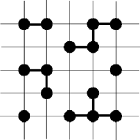
where $C_{s}^{q}=\langle s^{q}_{i}s^{q}_{j}\rangle_{G_{s}^{q}}$ is the spin two-point correlation of the $q-$level sample (see Fig. 1) and $\tilde{C}^{q}=\langle s^{q}_{i}s^{q}_{j}\rangle_{\tilde{G}}$ is the respective correlation over the entire grid. The $q-$level classification problem is equivalent to finding the optimal configuration $\hat{S}^{q}_{p}$ that minimizes (5):

$$\hat{S}^{q}_{p}=\operatorname*{arg\,min}_{S^{q}_{p}}U(S^{q}_{p}|S^{q}_{s}).$$ (6)

III.1.1 Monte Carlo Relaxation (Greedy Scheme)

Determining the optimum spin state is based on a Markov Chain Monte Carlo (MC) walk over the ensemble of possible spin configurations at sites that are not assigned a fixed class indicator value. The generation of new states is realized using Metropolis updating at $T=0.$ The zero-temperature condition means that there is no stochastic selection of unfavorable spins; i.e., the spin tested is flipped unconditionally if it lowers the cost function. This so-called “greedy” Monte Carlo algorithm (pap82, ) guarantees convergence, which is typically very fast. In contrast, in simulated annealing $T$ is slowly lowered from an initial high-temperature state. This approach is much slower computationally, but the resulting configuration is less sensitive to the initial state. The sensitivity of the greedy algorithm is pronounced in high-dimensional spaces with non-convex energies, since in such cases it is more likely to be trapped in local minima. However, this is not a concern in the current problem. In fact, targeting the global minimum of $U(S^{q}_{p}|S^{q}_{s})$ emphasizes exact matching of the sample correlation energy, which is subject to sample-to-sample fluctuations.

Figure 1: Schematic depicting the sample sites (solid circles) and the nearest-neighbor pairs (solid circles linked with bold lines) contributing to the sample correlation energy $C_{s}^{q}$.

III.1.2 Initial State Selection

To provide a fast and unsupervised automatic classification mechanism, the initial configuration of the spins at the prediction sites should require little or no user intervention and minimize the relaxation path to the equilibrium (in state space). Assuming a degree of spatial continuity, which is common in geospatial data sets, we propose to determine the initial states based on the sample values in the immediate neighborhood of the individual prediction points ${\vec{r}_{p}}$. More specifically, the initial spin states at the prediction sites are based on majority votes of the sample spins within an adaptable $m\times m$ stencil (where $m=2l+1$) centered at ${\vec{r}_{p}}$ . The stencil size $m\leq m_{\max}$ is set adaptively starting with $m=3$, reflecting the local sampling density and the spin values distribution, to the smallest size that contains a clear majority of spin values. Imposing the arbitrary upper bound $m_{\rm max}$ on the stencil size prevents oversmoothing and increasing the computational load (memory and CPU time). Intuitively, $m_{\rm max}$ should be higher for sparser sampling patterns. If a majority is not achieved for $m\leq m_{\rm max}$, the initial spin value is assigned at random from the sample spin values with the most votes. If a majority can not be achieved due to a lack of sampling points inside the maximum stencil, the initial value is drawn randomly from the entire range of spin values . We will refer to this procedure for determining the initial state as the adaptable stencil size (ASS) procedure. The indeterminacy of the initial state injects a stochastic element in the classification. Hence, by performing multiple initializations one can assess the classification uncertainty due to the initial state ambiguity.

The parametrization required by the algorithm involves only $m_{\max}$ and the definition of the class intervals. The number of classes depends on the study objective: if the goal is to determine areas where a specific level is exceeded, a binary classification is sufficient. For environmental monitoring and decision making purposes a moderate number of classes (e.g., eight) is often sufficient. A larger number of classes is necessary for the reconstruction of gray-scale images, and even larger numbers of classes are used for spatial interpolation.

III.1.3 Vectorized Algorithm for MC Simulation

On commensurate lattices, the grid structure and the short range of the interactions enable vectorization of the algorithm, thus improving the computational efficiency of the Monte Carlo relaxation. Vectorization is achieved by partitioning $\tilde{G}$ in two interpenetrating subgrids $\tilde{G}_{k},\ k=1,2$, so that the spins on one subgrid interact only with spins on the other. Hence, each subgrid can be updated simultaneously, while one sweep through the entire grid involves just two subgrid updating steps.

Starting from the initial state, Monte Carlo spin updating cycles are generated. Each cycle consists of two steps. Each step focuses on one sublattice, simultaneously generating updates for all the prediction sites. The updates are drawn uniformly from the set of possible values (e.g., $\pm 1$ for the Ising model, $1,\ldots,N_{c}$ for the Potts and clock models). The updates are accepted or rejected locally for each site, depending on whether they raise or lower the energy of the specific spin’s interactions. The algorithm proceeds until the cost function becomes zero within a specified tolerance (termination criterion I) or an updating cycle ends in rejection of all the updates (termination criterion II).

Based on the above, the vectorized Monte Carlo (MC) algorithm for the INNC classification model consists of the following steps:

Algorithm for INNC model

(1) Initialization
(1.1) Define $N_{c}$ and $m_{\max}$
(1.2) Set the indicator field on the entire grid by means of $\hat{I}_{Z}(\tilde{G})={\rm NaN}$
(2) Set the simulation level (class index) to $q=1$
(3) While [loop 1] $q\leq N_{c}-1$
(3.1) Define $S_{s}^{q}$ by discretizing $Z\{G_{s}\}$ with respect to $t_{q+1}$
(3.2) Assign spin values $S^{q}_{s}$ to the points on $G^{q}_{s}$
(3.3) Given the data $S^{q}_{s}$, calculate the sample correlation energy $C_{I;s}^{q}$
(3.4) Initialize spin values on $G^{q}_{p},$ based on ASS, i.e., generate $\hat{S}^{q\,(0)}_{p}$
(3.5) Given $S^{q}_{s}$ and $\hat{S}^{q\,(0)}_{p}$, calculate the initial simulated correlation energy $\tilde{C}_{I}^{q\,(0)}$
(3.6) Initialize the MC index $i_{mc}=0$ and the rejected states index $i_{r}=0$
(3.7) If $\tilde{C}_{I}^{q\,(0)}<C_{I;s}^{q}$
(3.7.1) While [loop 1.1] $(\tilde{C}_{I}^{q\,(i_{mc})}<C_{I;s}^{q}$) & $(i_{r}<2)$ update grid
Initialize the rejected states index $i_{r}=0$
For $k=1,2$ [subgrid updating]
(3.7.1.1)Generate a new state $\hat{S}^{q\,(i_{mc}+1)}_{p}$ by perturbing $\hat{S}^{q\,(i_{mc})}_{p}$ on subgrid $\tilde{G}_{k}$
(3.7.1.2)Identify prediction sites $\{i_{k}\}=K_{k}\subset\tilde{G}_{k}$, such that
$\{s_{i_{k}}\,s_{j}\}^{(i_{mc}+1)}>\{s_{i_{k}}\,s_{j}\}^{(i_{mc})}$
(3.7.1.3) If $K_{k}\neq\emptyset$ update the sites on $K_{k}$
else keep the “old” state  ; $\;i_{r}\rightarrow i_{r}+1$; endif
(3.7.1.4) $i_{mc}\rightarrow i_{mc}+1$
end [subgrid updating]
end [loop 1.1]
elseif $\tilde{C}_{I}^{q\,(0)}>C_{I;s}^{q}$
(3.7.2) While [loop 1.2] $(\tilde{C}_{I}^{q\,(i_{mc})}>C_{I;s}^{q}$) & $(i_{r}<2)$ update grid
Initialize the rejected states index $i_{r}=0$
For $k=1,2$ [subgrid updating]
(3.7.2.1)Generate a new state $\hat{S}^{q\,(i_{mc}+1)}_{p}$ by perturbing $\hat{S}^{q\,(i_{mc})}_{p}$ on subgrid $\tilde{G}_{k}$
(3.7.2.2)Identify prediction sites $\{i_{k}\}=K_{k}\subset\tilde{G}_{k}$, such that
$\{s_{i_{k}}\,s_{j}\}^{(i_{mc}+1)}<\{s_{i_{k}}\,s_{j}\}^{(i_{mc})}$
(3.7.2.3) If $K_{k}\neq\emptyset$ update the sites on $K_{k}$
  else keep the “old” state  ; $\;i_{r}\rightarrow i_{r}+1$; endif
(3.7.2.4) $i_{mc}\rightarrow i_{mc}+1$
end [subgrid updating]
end [loop 1.2]
else
$i_{mc}\rightarrow i_{mc}+1$
endif
(3.8) Assign the $-1$ spins to the $q$-th class, i.e.
$i_{mc}\rightarrow i_{mc}-1$;
If $\hat{S}^{q(i_{mc})}(\{\vec{r}_{i}\})=-1$, $\{\vec{r}_{i}\}\in\tilde{G},$ set $\hat{I}_{Z}(\{\vec{r}_{i}\})=q$
where $\hat{S}^{q(i_{mc})}(\{\vec{r}_{i}\}\in G_{s})\equiv S^{q}_{s}$; endif
(3.9) Increase the class index, $q\rightarrow q+1$, return to step (3)
end [loop 1]
(4) For $q=N_{c}$, $\forall\vec{r}_{i}\;(i=1,\ldots,N_{\tilde{G}})$ such that $\hat{I}_{Z}(\{\vec{r}_{i}\})={\rm NaN}$, set $\hat{I}_{Z}(\{\vec{r}_{i}\})=N_{c}\;$.

In the above, the symbol NaN denotes a non-numeric value used to initialize the class assignments. Loop 1 sequentially assigns values to each class. In loop 1.1 the sample energy is approached from below, while in loop 1.2 from above. In both cases the algorithm is vectorised by partitioning the lattice in two subgrids. The termination criterion requires that either the spin correlation energy match the sample energy (within machine precision) or that one sweep over entire grid not produce any successful updates. In steps 3.7.1.2 and 3.7.2.2 the terms $\{s_{i_{k}}\,s_{j}\}$ imply a summation over all the neighbor spins $s_{j}$ on the complementary subgrid for each $s_{i_{k}}$ on the perturbed subgrid. Step 3.8 assigns the $-1$ spins to the current class and adds the respective sites to the sampling set for the next higher level $q$. In the end, all the remaining spins with NaN values are assigned to the highest class.

III.2 Classification based on Multivalued Spin Models

This approach is based on models that involve multivalued spin variables with nearest neighbor correlations, such as the Potts, clock and XY Hamiltonians. The same algorithm structure is used for the nearest-neighbor correlation models based on the Potts (PNNC), clock (CNNC), and XY (XYNNC) models. The PNNC and CNNC models differ only in the form of the correlation energy, while the XYNNC differs from the CNNC model in the number of discretization levels. In contrast with the INNC model, the classification for the multi-valued models is performed simultaneously over all levels. Accordingly, we drop the index $q$ which refers to the current level, and the relevant quantities in the algorithm are calculated from the spin values $S=\{s_{i}\}$, $i=1,\ldots,N_{\tilde{G}}$ and $s_{i}\in\{1,\ldots,N_{c}\}$. The normalized correlation energies over the sample and entire grid are calculated by $C_{s}=\langle\delta_{(s_{i},s_{j})}\rangle_{G_{s}}$ and $\tilde{C}=\langle\delta_{(s_{i},s_{j})}\rangle_{\tilde{G}}$ for the PNNC model, and by $C_{s}=\left\langle\cos\left[\frac{\pi(s_{i}-s_{j})}{2N_{c}}\right]\right\rangle_{G_{s}}$ and $\tilde{C}=\left\langle\cos\Big{[}\frac{\pi(s_{i}-s_{j})}{2N_{c}}\Big{]}\right\rangle_{\tilde{G}}$ respectively for the CNNC and XYNNC models. Note that the prefactor in the argument of the cosine function is changed from $2\pi$ to $\pi/2$ to ensure that each energy level corresponds to a unique value of $|s_{i}-s_{j}|$. Based on the above, the MC algorithm for the PNNC models consists of the following steps:

Algorithm for PNNC model

(1) Initialization
(1.1) Define $N_{c}$ and $m_{\max}$
(1.2) Define $S_{s}$ by discretizing $Z\{G_{s}\}$ with respect to $t_{k},\ k=1,\ldots,N_{c}+1$
(1.3) Assign spin values $S_{s}$ to the points on $G_{s}$
(2) Given the data $S_{s}$, calculate the sample correlation energy $C_{P;s}$
(3) Initialize the spin values on $G_{p},$ based on ASS, i.e. generate $\hat{S}^{(0)}_{p}$
(4) Calculate the initial correlation $\tilde{C}_{P}^{(0)}$
(5) Initialize the MC index $i_{mc}=0$ and the rejected states index $i_{r}=0$
(6) If $\tilde{C}_{P}^{(0)}<C_{P;s}$
(6.1) While [loop 1] $(\tilde{C}_{P}^{(i_{mc})}<C_{P;s}$) & $(i_{r}<2)$ update grid
Initialize the rejected states index $i_{r}=0$
For $k=1,2$ [subgrid updating]
(6.1.1) Generate a new state $\hat{S}^{(i_{mc}+1)}_{p}$ by perturbing $\hat{S}^{(i_{mc})}_{p}$ on subgrid $\tilde{G}_{k}$
(6.1.2) Identify prediction sites $\{i_{k}\}=K_{k}\subset\tilde{G}_{k}$, such that
$\{\delta(s_{i_{k}},s_{j})\}^{(i_{mc}+1)}>\{\delta(s_{i_{k}},s_{j})\}^{(i_{mc})}$
(6.1.3) If $K_{k}\neq\emptyset$ update the sites on $K_{k}$
else keep the “old” state; $\;i_{r}\rightarrow i_{r}+1$; endif
(6.1.4) $i_{mc}\rightarrow i_{mc}+1$
end [subgrid updating]
end [loop 1]
elseif $\tilde{C}_{P}^{(0)}>C_{P;s}$
(6.2) While [loop 2] $(\tilde{C}_{P}^{(i_{mc})}>C_{P;s}$) & $(i_{r}<2)$ update grid
Initialize the rejected states index $i_{r}=0$
For $k=1,2$ [subgrid updating]
(6.2.1) Generate a new state $\hat{S}^{(i_{mc}+1)}_{p}$ by perturbing $\hat{S}^{(i_{mc})}_{p}$ on subgrid $\tilde{G}_{k}$
(6.2.2) Identify prediction sites $\{i_{k}\}=K_{k}\subset\tilde{G}_{k}$, such that
$\{\delta(s_{i_{k}},s_{j})\}^{(i_{mc}+1)}<\{\delta(s_{i_{k}},s_{j})\}^{(i_{mc})}$
(6.2.3) If $K_{k}\neq\emptyset$ update the sites on $K_{k}$
else keep the “old” state; $\;i_{r}\rightarrow i_{r}+1$; endif
(6.2.4) $i_{mc}\rightarrow i_{mc}+1$
end [subgrid updating]
end [loop 2]
else
$i_{mc}\rightarrow i_{mc}+1$
endif
(7)   $i_{mc}\rightarrow i_{mc}-1;$   assign $\hat{I}_{Z}(\{\vec{r}_{i}\})=\hat{S}^{(i_{mc})}(\{\vec{r}_{i}\})$, $\{\vec{r}_{i}\}\in\tilde{G}$, where $\hat{S}^{(i_{mc})}(\{\vec{r}_{i}\}\in G_{s})\equiv S_{s}$.

The main difference with the INNC case is the absence of a loop over different classes since the initial spin discretization corresponds to the number of classes.

IV Classification of Simulated Random Field Data

IV.1 Simulation Study Design

We study the performance of the classification models on simulated realizations of Gaussian, $Z\sim N(m=50,\sigma=10)$, and lognormal, $\ln Z\sim N(m=4,\sigma=0.5)$ random fields yagl87 . The spatial correlations are imposed by means of the flexible Whittle-Matérn family of covariance functions:

$$G_{\rm Z}(\|\vec{r}\|)=\sigma^{2}\frac{{2}^{1-\nu}}{\Gamma(\nu)}(\kappa\,\|\vec{r}\|)^{\nu}K_{\nu}(\kappa\,\|\vec{r}\|),$$ (7)

where $\|\vec{r}\|$ is the Euclidean two-point distance, $\sigma^{2}$ is the variance, $\nu$ is the smoothness parameter, $\kappa$ is the inverse autocorrelation length, and $K_{\nu}$ is the modified Bessel function of index $\nu$. This $G_{\rm Z}(\|\vec{r}\|)$ leads to random field realizations that are $m$ times differentiable, where $m$ is the largest integer smaller than $\nu.$ In addition, higher values of $\kappa$ imply shorter correlation ranges. We generate samples with different combinations of $\kappa=0.2,\ 0.5$ and $\nu=1.5,\ 2.5$ on a square ($L_{x}=L_{y}=L$) grid $\tilde{G}$, with $N_{G}=L^{2}$ nodes, where $L=50,\ 100,\ 200$. The samples are generated using the spectral method drum87 ; hrist02 . From the complete data set on $\tilde{G}$, we extract a sample $Z_{s}$ of size $N=(1-p)\,N_{G}$ by randomly removing $P=pN_{G}$ points for validation. For different degrees of thinning ($p=0.33$ and $0.66$), we generate $100$ different configurations of $G_{p}$. We use two values of class numbers ($N_{c}=8$ and $16$), corresponding to different discretizations of the continuum (resolutions). The simulated values on $G_{p}$ are classified using the spin-based algorithms. In the classification performance evaluation, the indicator field values $I_{Z}(G_{p})$ are compared with the estimates $\hat{I}_{Z}(G_{p})$ that were obtained from the classification algorithms. We define the misclassification rate as

$$F=\frac{1}{P}\sum_{p=1}^{P}\left[1-\delta\big{(}I_{Z}(\vec{r}_{p}),\hat{I}_{Z}(\vec{r}_{p})\big{)}\right],$$ (8)

where $I_{Z}(\vec{r}_{p})$ is the true value at the validation points, $\hat{I}_{Z}(\vec{r}_{p})$ is the classification estimate and $\delta(I,I^{\prime})=1$ if $I=I^{\prime}$, $\delta(I,I^{\prime})=0$ if $I\neq I^{\prime}$. We also measure the optimization CPU time, $T_{\rm cpu}$, the number of MC sweeps required for reaching equilibrium, and the residual values of the cost function at termination, $U^{\ast}$.

To evaluate the performance of the spin models for large $N_{c}$ (i.e., approaching the continuum limit), we calculate the following “sample” prediction errors: average absolute error AAE $=\frac{1}{P}\sum_{p=1}^{P}|Z(\vec{r}_{p})-\hat{Z}(\vec{r}_{p})|$, average relative error ARE $=\frac{1}{P}\sum_{p=1}^{P}\frac{Z_{p}-\hat{Z_{p}}}{Z_{p}}$, average absolute relative error AARE $=\frac{1}{P}\sum_{p=1}^{P}\bigg{|}\frac{Z(\vec{r}_{p})-\hat{Z}(\vec{r}_{p})}{Z(\vec{r}_{p})}\bigg{|}$, root average square error RASE $=\sqrt{\sum_{p=1}^{P}\frac{1}{P}|Z(\vec{r}_{p})-\hat{Z}(\vec{r}_{p})|^{2}}$, and the linear sample correlation coefficient $R$. In the above definitions, $P$ is the number of validation points, $Z(\vec{r}_{p})$ is the true value at $\vec{r}_{p}$ and $\hat{Z}(\vec{r}_{p})$ is the estimate of the process based on

$$\hat{Z}(\vec{r}_{p})=t_{\hat{I}_{Z}(\vec{r}_{p})}+\frac{t_{\hat{I}_{Z}(\vec{r}_{p})+1}-t_{\hat{I}_{Z}(\vec{r}_{p})}}{2}.$$ (9)

To focus on local behavior of the classifiers we define the respective errors, in which the spatial average is replaced by a mean value calculated over a number of samples (e.g. $M=100$ realizations) at each point. Namely, at point $p$, mean absolute error = $\langle|Z(\vec{r}_{p})-\hat{Z}_{j}(\vec{r}_{p})|\rangle$, mean relative error = $\bigg{\langle}\frac{Z(\vec{r}_{p})-\hat{Z}_{j}(\vec{r}_{p})}{Z(\vec{r}_{p})}\bigg{\rangle}$, mean absolute relative error = $\bigg{\langle}\bigg{|}\frac{Z(\vec{r}_{p})-\hat{Z}_{j}(\vec{r}_{p})}{Z(\vec{r}_{p})}\bigg{|}\bigg{\rangle}$, and root mean squared error = $\sqrt{\langle|Z(\vec{r}_{p})-\hat{Z}_{j}(\vec{r}_{p})|^{2}\rangle}$, where $\hat{Z}_{j}(\vec{r}_{p})$ are predictions at point $p$ obtained from $j=1,...,M$ realizations and $\langle.\rangle$ denotes averaging over different realizations. The computations are performed in the Matlab® programming environment on a desktop computer with 1.93 GB of RAM and an Intel®Core™2 CPU 6320 processor with an 1.86 GHz clock.

IV.2 Misclassification rate

We investigate the effects of grid size $N_{G}$, data sparseness $p$, and class number $N_{c}$ on the classification performance. The results obtained by the INNC, PNNC, and CNNC models are compared with the best results obtained by the established KNN and FKNN methods (see II.1). Tables 1-3 summarize the results obtained for Gaussian random fields with Whittle-Matérn parameters $(\kappa,\nu)=(0.2,2.5)$, $(0.5,2.5)$, and $(0.5,1.5)$, respectively. Table 4 lists the results obtained from lognormal random fields with Whittle-Matérn parameters $(\kappa,\nu)=(0.5,2.5)$.

Table 1: Classification results using the 8- and 16-level INNC, PNNC, and CNNC models for realizations of Gaussian random fields $\sim N(50,10)$ with Whittle-Matérn covariance ($\kappa=0.2,\nu=2.5$) on a square domain of size $L$. The tabulated results are averages over $100$ realizations. They include the mean value and standard deviation of the misclassification rate $\langle F^{*}\rangle$ and $\mbox{STD}_{F^{*}}$ ($\%$), the mean number of Monte Carlo sweeps $\langle N_{MC}\rangle$, the mean optimization CPU time $\langle T_{\rm cpu}\rangle$ $[sec]$, and the mean value of the cost function at termination $\langle U^{*}\rangle$. The $\langle F^{*}_{\rm knn}\rangle$ and $\langle F^{*}_{\rm fknn}\rangle$ represent the mean of the lowest misclassification rates $[\%]$ achieved by KNN and FKNN algorithms respectively.

Size	L=50						L=100						L=200
Model	INNC		PNNC		CNNC		INNC		PNNC		CNNC		INNC		PNNC		CNNC
$p[\%]$	$33$	$66$	$33$	$66$	$33$	$66$	$33$	$66$	$33$	$66$	$33$	$66$	$33$	$66$	$33$	$66$	$33$	$66$
$N_{c}=8$
$\langle F^{*}_{\rm knn}\rangle$	13.6	20.4	$-$	$-$	$-$	$-$	10.3	16.1	$-$	$-$	$-$	$-$	8.2	12.8	$-$	$-$	$-$	$-$
$\langle F^{*}_{\rm fknn}\rangle$	12.4	18.1	$-$	$-$	$-$	$-$	9.5	14.5	$-$	$-$	$-$	$-$	7.6	11.6	$-$	$-$	$-$	$-$
$\langle F^{*}\rangle$	11.1	16.1	12.9	19.1	12.4	17.5	8.6	12.9	9.6	14.9	9.5	14.0	6.9	10.6	7.4	11.7	7.3	11.1
${\rm STD}_{F^{*}}$	1.25	1.03	1.34	1.10	1.18	1.02	0.52	0.43	0.56	0.43	0.52	0.45	0.24	0.22	0.26	0.23	0.26	0.21
$\langle N_{MC}\rangle$	4.4	6.2	2.7	6.0	3.4	8.5	6.3	6.9	5.5	9.1	5.0	12.5	6.8	8.0	9.5	13.7	9.9	17.4
$\langle T_{\rm cpu}\rangle$	0.11	0.33	0.03	0.11	0.05	0.13	0.47	1.72	0.13	0.44	0.20	0.61	2.02	7.11	0.61	1.99	1.06	2.95
$\langle U^{*}\rangle$	5e-4	2e-3	3e-5	1e-4	8e-9	4e-8	3e-4	1e-3	5e-6	2e-5	2e-9	1e-8	1e-4	6e-4	1e-6	4e-6	3e-10	2e-9
$N_{c}=16$
$\langle F^{*}_{\rm knn}\rangle$	34.2	40.2	$-$	$-$	$-$	$-$	27.7	34.2	$-$	$-$	$-$	$-$	20.7	28.0	$-$	$-$	$-$	$-$
$\langle F^{*}_{\rm fknn}\rangle$	31.9	38.9	$-$	$-$	$-$	$-$	25.3	32.7	$-$	$-$	$-$	$-$	18.9	25.9	$-$	$-$	$-$	$-$
$\langle F^{*}\rangle$	21.2	33.8	35.1	42.8	23.5	31.5	17.2	27.3	27.9	35.8	21.2	28.4	13.6	21.5	20.5	28.0	18.2	24.7
${\rm STD}_{F^{*}}$	1.48	1.60	1.64	1.24	1.52	1.56	0.67	0.75	0.85	0.52	0.73	0.83	0.31	0.36	0.35	0.29	0.38	0.74
$\langle N_{MC}\rangle$	8.5	12.9	6.5	17.0	35.1	45.1	13.1	15.2	4.2	14.7	39.6	43.3	13.9	17.1	3.2	2.8	47.5	46.7
$\langle T_{\rm cpu}\rangle$	0.22	0.62	0.05	0.14	0.18	0.32	0.94	3.30	0.15	0.55	0.84	1.28	3.85	13.92	0.55	1.82	4.02	5.32
$\langle U^{*}\rangle$	7e-4	2e-3	1e-4	5e-4	2e-9	1e-9	4e-4	1e-3	2e-7	4e-6	3e-11	4e-11	2e-4	8e-4	6e-8	5e-7	1e-12	3e-12

Table 2: The same classification statistics are listed as in Table 1, obtained from realizations of a Gaussian random field with Whittle-Matérn covariance ($\kappa=0.5,\nu=2.5$).

Size	L=50						L=100						L=200
Model	INNC		PNNC		CNNC		INNC		PNNC		CNNC		INNC		PNNC		CNNC
$p[\%]$	$33$	$66$	$33$	$66$	$33$	$66$	$33$	$66$	$33$	$66$	$33$	$66$	$33$	$66$	$33$	$66$	$33$	$66$
$N_{c}=8$
$\langle F^{*}_{\rm knn}\rangle$	25.6	32.3	$-$	$-$	$-$	$-$	25.8	32.6	$-$	$-$	$-$	$-$	21.8	28.8	$-$	$-$	$-$	$-$
$\langle F^{*}_{\rm fknn}\rangle$	23.5	30.3	$-$	$-$	$-$	$-$	23.7	30.6	$-$	$-$	$-$	$-$	20.2	26.7	$-$	$-$	$-$	$-$
$\langle F^{*}\rangle$	19.7	27.5	25.6	32.3	22.2	28.7	19.4	27.0	24.9	32.5	22.2	28.8	17.2	23.7	21.2	28.1	19.4	25.5
${\rm STD}_{F^{*}}$	1.36	1.23	1.63	1.19	1.56	1.33	0.74	0.69	0.85	0.63	0.76	0.71	0.34	0.30	0.43	0.27	0.33	0.29
$\langle N_{MC}\rangle$	5.0	6.2	6.6	12.5	7.8	7.9	5.8	7.7	14.6	23.3	6.5	7.9	5.9	8.6	13.0	19.4	6.0	6.6
$\langle T_{\rm cpu}\rangle$	0.11	0.35	0.04	0.12	0.07	0.14	0.46	1.60	0.18	0.56	0.24	0.53	1.90	6.62	0.74	2.30	0.87	2.07
$\langle U^{*}\rangle$	7e-4	2e-3	1e-4	7e-4	9e-10	2e-9	6e-4	2e-3	3e-5	2e-4	3e-10	1e-9	4e-4	2e-3	5e-7	4e-6	1e-10	6e-10
$N_{c}=16$
$\langle F^{*}_{\rm knn}\rangle$	51.9	55.4	$-$	$-$	$-$	$-$	53.9	56.5	$-$	$-$	$-$	$-$	48.1	51.4	$-$	$-$	$-$	$-$
$\langle F^{*}_{\rm fknn}\rangle$	49.7	54.7	$-$	$-$	$-$	$-$	51.5	56.1	$-$	$-$	$-$	$-$	45.4	50.9	$-$	$-$	$-$	$-$
$\langle F^{*}\rangle$	39.0	54.0	52.7	58.5	37.2	48.7	38.7	53.9	52.9	59.3	36.2	48.1	33.7	48.1	46.9	54.1	32.7	44.1
${\rm STD}_{F^{*}}$	1.77	1.55	1.55	1.00	2.30	1.69	0.87	0.76	0.77	0.54	1.34	0.96	0.47	0.42	0.41	0.24	0.55	0.44
$\langle N_{MC}\rangle$	10.3	12.7	19.1	27.3	23.1	19.9	11.6	14.3	39.7	50.1	23.3	20.6	11.9	16.8	59.6	70.4	24.4	21.5
$\langle T_{\rm cpu}\rangle$	0.21	0.65	0.07	0.17	0.14	0.21	0.91	2.99	0.34	0.88	0.57	0.85	3.78	12.44	1.90	4.69	2.41	3.57
$\langle U^{*}\rangle$	8e-4	2e-3	2e-3	2e-2	9e-11	3e-10	7e-4	2e-3	2e-3	2e-2	2e-11	1e-10	5e-4	2e-3	3e-4	7e-3	1e-11	7e-11

Table 3: The same classification statistics are listed as in Table 1, obtained from realizations of a Gaussian random field with Whittle-Matérn covariance ($\kappa=0.5,\nu=1.5$).

Size	L=50						L=100						L=200
Model	INNC		PNNC		CNNC		INNC		PNNC		CNNC		INNC		PNNC		CNNC
$p[\%]$	$33$	$66$	$33$	$66$	$33$	$66$	$33$	$66$	$33$	$66$	$33$	$66$	$33$	$66$	$33$	$66$	$33$	$66$
$N_{c}=8$
$\langle F^{*}_{\rm knn}\rangle$	38.9	44.8	$-$	$-$	$-$	$-$	36.7	42.4	$-$	$-$	$-$	$-$	30.7	37.1	$-$	$-$	$-$	$-$
$\langle F^{*}_{\rm fknn}\rangle$	36.7	42.9	$-$	$-$	$-$	$-$	34.6	40.6	$-$	$-$	$-$	$-$	28.9	34.9	$-$	$-$	$-$	$-$
$\langle F^{*}\rangle$	31.7	39.5	38.6	45.0	35.9	42.8	29.5	37.2	36.0	42.4	33.9	40.2	25.6	32.0	29.7	36.1	29.9	35.4
${\rm STD}_{F^{*}}$	1.66	1.31	1.59	1.14	1.71	1.10	0.79	0.68	0.69	0.57	0.78	0.75	0.37	0.32	0.36	0.28	0.39	0.30
$\langle N_{MC}\rangle$	3.9	5.5	12.2	16.9	3.4	3.2	4.1	6.6	21.9	27.5	3.2	3.2	4.2	7.3	29.6	37.2	0.76	1.3
$\langle T_{\rm cpu}\rangle$	0.12	0.36	0.05	0.14	0.05	0.11	0.48	1.62	0.22	0.64	0.18	0.45	1.98	6.76	1.05	2.86	0.53	1.69
$\langle U^{*}\rangle$	9e-4	3e-3	3e-3	1e-2	4e-9	2e-8	7e-4	3e-3	1e-3	7e-3	2e-9	1e-8	4e-4	2e-3	8e-4	4e-3	1e-9	8e-9
$N_{c}=16$
$\langle F^{*}_{\rm knn}\rangle$	64.8	67.3	$-$	$-$	$-$	$-$	63.5	65.7	$-$	$-$	$-$	$-$	58.5	61.0	$-$	$-$	$-$	$-$
$\langle F^{*}_{\rm fknn}\rangle$	63.2	66.6	$-$	$-$	$-$	$-$	61.4	65.1	$-$	$-$	$-$	$-$	56.3	60.5	$-$	$-$	$-$	$-$
$\langle F^{*}\rangle$	54.8	65.8	65.1	69.4	56.7	64.5	53.3	64.8	62.2	67.3	54.8	62.9	47.9	58.4	57.3	62.7	50.8	58.6
${\rm STD}_{F^{*}}$	1.71	1.34	1.46	1.07	1.77	1.24	0.89	0.76	0.78	0.54	0.89	0.67	0.44	0.34	0.42	0.28	0.50	0.37
$\langle N_{MC}\rangle$	8.6	11.0	21.0	29.8	9.2	8.2	8.7	12.4	40.5	51.9	9.2	7.9	8.9	13.8	61.3	73.2	8.9	7.8
$\langle T_{\rm cpu}\rangle$	0.23	0.67	0.07	0.18	0.09	0.15	0.94	3.09	0.36	0.91	0.32	0.61	3.96	12.78	1.84	4.76	1.28	2.49
$\langle U^{*}\rangle$	8e-4	2e-3	2e-2	1e-1	9e-10	4e-9	7e-4	2e-3	1e-2	9e-2	6e-10	3e-9	5e-4	2e-3	8e-3	6e-2	3e-10	2e-9

Table 4: The same classification statistics are listed as in Table 1, obtained from realizations of a lognormal random field with Whittle-Matérn covariance ($\kappa=0.5,\nu=2.5$).

Size	L=50						L=100						L=200
Model	INNC		PNNC		CNNC		INNC		PNNC		CNNC		INNC		PNNC		CNNC
$p[\%]$	$33$	$66$	$33$	$66$	$33$	$66$	$33$	$66$	$33$	$66$	$33$	$66$	$33$	$66$	$33$	$66$	$33$	$66$
$N_{c}=8$
$\langle F^{*}_{\rm knn}\rangle$	18.7	24.3	$-$	$-$	$-$	$-$	21.5	27.5	$-$	$-$	$-$	$-$	16.5	22.3	$-$	$-$	$-$	$-$
$\langle F^{*}_{\rm fknn}\rangle$	17.3	22.3	$-$	$-$	$-$	$-$	19.9	25.4	$-$	$-$	$-$	$-$	15.3	20.3	$-$	$-$	$-$	$-$
$\langle F^{*}\rangle$	15.2	20.9	18.4	23.8	16.3	21.6	16.8	23.1	20.6	26.6	18.2	24.0	13.7	18.8	15.6	20.9	14.9	19.8
${\rm STD}_{F^{*}}$	1.29	1.17	1.31	0.95	1.15	1.13	0.70	0.63	0.76	0.52	0.67	0.61	0.30	0.30	0.35	0.31	0.31	0.31
$\langle N_{MC}\rangle$	3.7	4.6	6.0	10.0	7.0	8.4	4.5	5.7	15.0	20.3	6.9	7.1	4.6	6.5	19.5	20.6	5.1	5.3
$\langle T_{\rm cpu}\rangle$	0.08	0.19	0.04	0.12	0.07	0.14	0.32	0.87	0.18	0.57	0.24	0.53	1.26	3.27	0.86	2.34	0.83	2.28
$\langle U^{*}\rangle$	6e-4	1e-3	1e-4	7e-4	6e-9	7e-9	6e-4	2e-3	4e-5	2e-4	2e-10	9e-10	3e-4	1e-3	4e-6	8e-6	8e-11	6e-10
$N_{c}=16$
$\langle F^{*}_{\rm knn}\rangle$	37.1	41.7	$-$	$-$	$-$	$-$	42.7	47.1	$-$	$-$	$-$	$-$	35.1	40.2	$-$	$-$	$-$	$-$
$\langle F^{*}_{\rm fknn}\rangle$	34.9	40.0	$-$	$-$	$-$	$-$	40.4	45.8	$-$	$-$	$-$	$-$	33.1	38.7	$-$	$-$	$-$	$-$
$\langle F^{*}\rangle$	28.8	37.9	37.0	42.4	29.7	37.1	32.0	42.2	41.7	48.5	31.5	41.4	26.1	35.1	34.0	40.8	27.2	35.6
${\rm STD}_{F^{*}}$	1.85	1.43	1.62	1.07	1.73	1.41	0.96	0.79	0.75	0.56	1.15	0.74	0.35	0.40	0.37	0.30	0.46	0.42
$\langle N_{MC}\rangle$	8.9	10.4	13.8	21.4	18.8	18.8	10.3	12.5	35.7	45.3	19.9	17.5	10.8	14.1	52.1	63.9	19.7	17.2
$\langle T_{\rm cpu}\rangle$	0.16	0.33	0.06	0.16	0.12	0.20	0.61	1.53	0.31	0.84	0.54	0.84	2.35	5.7	1.63	4.31	2.14	3.44
$\langle U^{*}\rangle$	7e-4	2e-3	8e-4	6e-3	2e-9	2e-10	7e-4	2e-3	7e-4	6e-3	3e-11	2e-10	5e-4	2e-3	1e-4	2e-3	9e-12	7e-11

As expected, the misclassification rate overall decreases with increasing $N_{G}$ and increases proportionally with $p$. Comparing the performance of different models at fixed $N_{G}$, $p$, $N_{c}$ and distributional assumptions, the INNC model performs uniformly better for $N_{c}=8$. For $N_{c}=16$ and $(\kappa,\nu)=(0.2,2.5)$, the INNC model gives in general the lowest $\langle F^{*}\rangle$, except one case in which the CNNC model performs best. Generally, the CNNC model is expected to perform better when the cross-class correlations make finite contributions to the correlation energy. This is likely as the number of classes or the spatial variation of the data increase. The case of $N_{c}=16$ and $(\kappa,\nu)=(0.5,2.5)$ provides an example combining higher $N_{c}$ and shorter-range variations than $N_{c}=8$ and $\kappa=0.2$. This example shows a clear advantage of the CNNC model (especially at $p=0.66$) over the others. However, since the interactions are restricted to nearest neighbors, cross-class correlations in CNNC can increase the sensitivity to noisy or “rough” data. This is evidenced in the $N_{c}=16$ case for $(\kappa,\nu)=(0.5,1.5)$. The random field realizations for $\nu=1.5$ are only once differentiable, in contrast with the $\nu=2.5$ case, where the realizations are twice differentiable. For $\nu=1.5$ the classification performance of the CNNC model approaches that of the INNC model. The highest misclassification rate among the spin models investigated is displayed consistently by the PNNC model. This could be attributed to the fact that it incorporates less information than its counterparts. Namely, the INNC model sequentially uses the lower level classification results in the higher level estimates. On the other hand, the CNNC model differentiates between neighbors of various classes. In contrast, the PNNC model can only distinguish if the neighbors belong to the same or different classes. As we show below, the Potts model leads to degenerate states, which are undesirable for classification purposes.

IV.3 Impact of Initial State Selection

Fig. 2 illustrates the behavior of the misclassification rates, $F^{\ast}$, and the CPU times versus $m_{\rm max}$, considering fixed (FSS) and adaptable (ASS) stencil size approaches. Relatively small $m_{\rm max}=5,7$, for FSS and ASS respectively, lead to the lowest $F^{\ast}$ values. The computational time increases quadratically with $m_{\rm max}$. There is no significant difference in computational time between the two methods. However, using ASS leads to a significantly lower misclassification rate.

(a) Misclassification rate

(b) CPU time

Figure 2: (Color online) Dependence of misclassification rate, $F^{\ast},$ on the maximum stencil size $m_{\rm max}$ used in the initialization with both adaptable and fixed stencil size (a). Dependence of the CPU time on $m_{\rm max}$ (b). The 16-class INNC model is applied to a sample generated from a realization of a Gaussian random field with Whittle-Matérn covariance ($\kappa=0.5$, $\nu=1.5$) on a square grid ($L=200$) by removing $66\%$ of the points.

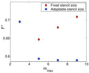
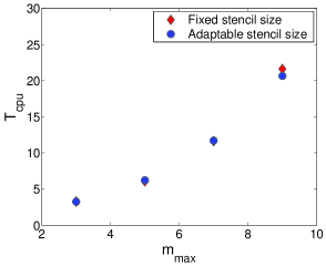
For the results obtained in Tables (1)-(4), the initial state was based on majority vote with ASS. This accelerates the relaxation process and prevents trapping in a “poor” local minimum. To test the sensitivity of the spin models on different initial states, we repeat the simulations using randomly assigned initial states for Gaussian data with $(\kappa,\nu)=(0.5,2.5)$ on a $L=200$ grid. The results for different models and two values of $N_{c}$ are given in Table 5. The greatest impact on the classification performance is observed for the INNC model. On the other hand, the CNNC model is the most robust with respect to changes of the initial state, especially for lower $p$ and higher $N_{c}$. For instance, at $p=0.33$ and $N_{c}=16$, there is practically no difference between the misclassification rates obtained using initial states based on random versus ASS majority rule selection of the spins. Using a random initial state increases by $73\%$ the number of MC sweeps needed to achieve equilibrium. However, the CPU time is increased only by $17\%$, because the random assignment strategy leads to faster determination of the initial state.

Table 5: Classification results using the 8- and 16-level INNC, PNNC, and CNNC models for realizations of a Gaussian random field $\sim N(50,10)$ with Whittle-Matérn covariance $(\kappa=0.5,\nu=2.5)$ and $L=200$. The simulations start from random initial states. The same statistics are listed as in Table 1.

	$N_{c}=8$						$N_{c}=16$
Model	INNC		PNNC		CNNC		INNC		PNNC		CNNC
$p[\%]$	$33$	$66$	$33$	$66$	$33$	$66$	$33$	$66$	$33$	$66$	$33$	$66$
$\langle F^{*}\rangle$	34.3	91.3	25.6	42.5	22.0	36.3	67.1	98.8	56.5	69.8	32.7	49.4
${\rm STD}_{F^{*}}$	0.50	0.20	0.34	0.43	0.37	0.47	18.3	0.07	0.40	0.43	0.59	0.64
$\langle N_{MC}\rangle$	7.0	3.0	27.3	74.9	31.7	68.9	13.1	5.2	23.3	32.3	42.4	49.8
$\langle T_{\rm cpu}\rangle$	1.15	1.24	0.63	2.54	2.12	4.92	2.28	2.0	0.53	1.16	2.82	3.73
$\langle U^{*}\rangle$	1e-1	1e-1	2e-7	8e-4	2e-11	3e-8	9e-2	6e-2	4e-6	3e-6	9e-12	4e-11

IV.4 Spatial Degeneracy

The higher sensitivity of the INNC model to the initial state is due to the sequential spin estimation, which propagates the misclassification from lower to higher levels, thus resulting in a higher overall misclassification rate. The misclassification at lower levels can occur due to the presence of degenerate states which correspond to different spatial configurations, even though their energies are numerically identical. Generally, the degeneracy increases with $p$, as a result of relaxing the spatial constraints. As the size of the prediction set is reduced at higher levels, due to the inclusion of the classified lower levels in the sampling set, the degeneracy is accordingly diminished. However, the lower level misclassifications propagate to higher levels. A high level of degeneracy is also responsible for the relatively poor classification performance of the PNNC model; since the latter does not include cross-class correlations, the energy contributions of all the nearest neighbor pairs that do not belong in the same class are zero. We believe that the robustness of the CNNC model and its competitive classification performance is partially due to the reduction of degeneracy achieved by differentiating between the energy contributions of neighbors belonging to different classes.

Table 6: Degeneracy and residual values of the cost function corresponding to 100 random initial states. The sample is a realization of a Gaussian random field $\sim N(50,10)$ with Whittle-Matérn covariance $(\kappa=0.5,\nu=2.5)$ on a grid of size $L=50$.

	$N_{c}=8$						$N_{c}=16$
Model	INNC		PNNC		CNNC		INNC		PNNC		CNNC
$p[\%]$	$33$	$66$	$33$	$66$	$33$	$66$	$33$	$66$	$33$	$66$	$33$	$66$
degeneracy	6	8	77	10	64	7	8	4	61	53	6	0
$\langle U^{*}\rangle$	8e-2	1e-1	7e-7	4e-4	1e-10	7e-9	8e-2	6e-2	4e-6	5e-6	5e-11	1e-10

(a) $p=0.33$

(b) $p=0.66$

Figure 3: (Color online) Histograms of the residual values of the cost function obtained from the PNNC model for one sampling realization and 100 different random initial states, with $N_{c}=8$ and different values of $p$. Each bar may include states with similar but not identical values of the cost function due to finite bar width. Note different scales of the abscissas.

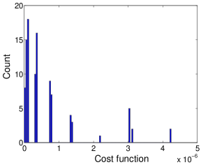
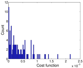
To investigate the degeneracy of the final class configurations obtained by the different spin models, we use the same sampling configuration on a grid of size $L=50$. We then run the MC simulation for $100$ different (randomly assigned) sets of initial values at the prediction points. We measure the degeneracy as the number of final configurations (states) with the same residual cost function value as at least one other state from which they differ in the misclassification rate. The results are summarized in Table 6. Note that for the INNC model, the degenerate states only appear at the first ($q=1$) level. The highest degeneracy is observed in the PNNC model. The histograms of the residual cost function value obtained for the PNNC model at $p=0.33$ and $p=0.66$ are shown in Fig. 3. Intuitively, one would expect the degeneracy to increase with $p$. However, the opposite tendency is observed in the simulations. The overall shift of $\langle U^{*}\rangle$ to higher values and the shape of the histogram (Fig. 3) suggest that the reduction of degeneracy is due to a scattering of energy levels. This can be viewed as a result of the cost function developing multiple local minima (multimodality). A reduction of the degeneracy is also observed with increasing $L$: for example, the configurations produced by the CNNC model for $L=200$ do not exhibit spatial degeneracy for any of the $N_{c}$ and $p$ combinations tested.

Figure 4: (Color online) Cost function evolution versus the number of full (over the entire grid) MC sweeps. Ten initial states are generated by the majority rule with adaptable stencil size, leading to ten $U^{\ast}$ evolution curves. The curves are based on the 8-class PNNC model simulations performed on a single realization of a Gaussian random field $(\kappa=0.5,\nu=2.5)$ on a grid of size $L=50$ from which $33\%$ of the points are randomly removed.

IV.5 Classification Uncertainty

(a) Cost function (PNNC, $L=50$)

(b) Misclass. rate (PNNC, $L=50$)

(c) Cost function (CNNC, $L=200$)

(d) Misclass. rate (CNNC, $L=200$)

Figure 5: (Color online) Residual values of the cost function at termination, $U^{\ast},$ and the misclassification rate, $F^{\ast},$ for the 8-class PNNC model, (a), (b) and for the 8-class CNNC model (c), (d). The sample is obtained from one realization of a Gaussian random field with Whittle-Matérn parameters ($\kappa=0.5,\nu=2.5$) on grids of size $L=50$ (PNNC) and $L=200$ (CNNC) respectively, by randomly removing $p=0.33$ of the points. The $U^{\ast},F^{\ast}$ values are obtained from 100 initial states generated by the majority rule with adaptable stencil size.

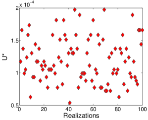
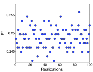
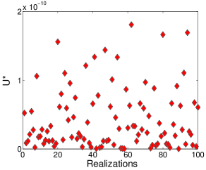
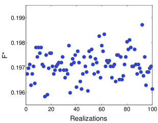
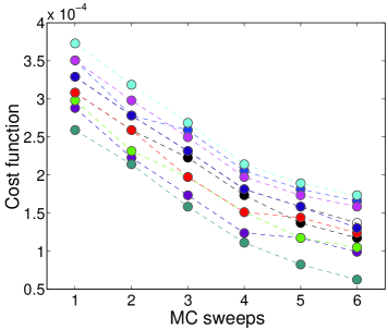
Multimodality and degeneracy introduce an uncertainty in the classification outcome, starting from different initial states. The cost function multimodality persists, even in cases where the degeneracy vanishes. An additional source of uncertainty is termination criterion II: if the relaxation process stops before the (local) optimum is reached, the final configuration depends on the initial state, thus mimicking multimodality of the cost function. Termination criterion II is arbitrary and aims at computational efficiency. Hence, it does not guarantee that the resulting configuration is in a perfect (quasi-)equilibrium state. Uncertainty is primarily generated by the ASS random initial assignment of those prediction points for which majority rule is not established. Fig. 4 demonstrates the cost function evolution during the relaxation process. We use the 8-class PNNC model classification on a single realization of a Gaussian random field ($\kappa=0.5,\nu=2.5)$ on a grid of size $L=50$ (high spatial degeneracy) thinned by $33\%$. The ten curves correspond to initial states generated by the majority rule with ASS. Different initial states follow different relaxation paths, leading to different local minima (based on the current value of termination criterion II). Figs. 5(a) and 5(b) are respectively the residual values of the cost function at termination and the misclassification rates for the 8-class PNNC model, obtained from $100$ different initial states generated by the majority rule with ASS. Figs. 5(c) and 5(d) show the same quantities as Figs. 5(a) and 5(b), but for $L=200$ using the 8-class CNNC model (for which no degeneracy was observed). In both cases, the resulting values vary, with the variations being more pronounced in the degenerate case.

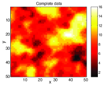
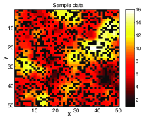
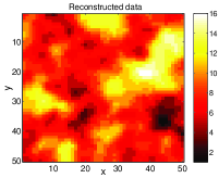
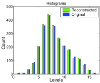
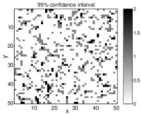
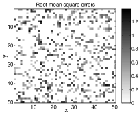
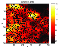
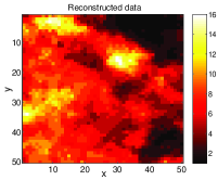
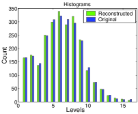
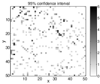
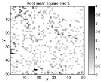
In light of the above, the spin-based classification methods permit the estimation of the classification uncertainty by sampling over different initial configurations. This allows us to determine points in space with increased chance of misclassification. Therefore, multiple Monte Carlo runs starting from different initial states permit statistical estimates. This repetitive application can also improve estimation results compared to a single run. For example, we consider one sample realization of a Gaussian random field with $\kappa=0.5$, $\nu=2.5$, on a grid of size $L=50$ reduced by $p=0.33$. A single simulation run using the 16-class CNNC model gave a misclassification rate of $F^{*}=36.6\%$. Repeating the simulation $100$ times, the median misclassification rate drops to $F^{*}=30.1\%$. The total CPU time increases linearly with the number of runs, leading to $T_{\rm cpu}=14.8$ seconds. We note that comparable results can be also obtained with significantly fewer simulation runs, e.g., $10$. Fig. 6(a) shows the complete realization, Fig. 6(b) the sample with the missing data points, and Fig. 6(c) the reconstructed image based on the medians of the estimates from the 100 runs. There is good visual agreement between the original and the reconstructed images. The class histogram of the reconstruction also matches satisfactorily that of the data, both shown in Fig. 6(d). Note that both histograms are asymmetric, even though the random field values are normally distributed. This is due to the relatively long correlation length that results in relatively more areas of higher than lower values as shown in Fig 6(a). Finally, Fig. 6(e) displays maps representing the width of the $95\%$ class confidence interval and Fig. 6(f) the class root mean square error at each prediction point.

(a) Original

(b) Sample

(c) Reconstructed

(d) Histograms

(e) Conf. interval

(f) RMSE

Figure 6: (Color online) Classification results obtained from the 16-class CNNC model. The sample is obtained from one realization of a Gaussian random field with Whittle-Matérn parameters ($\kappa=0.5,\nu=2.5$) on a grid of size $L=50$ by randomly removing $p=0.33$ of the points. One hundred reconstructions are generated starting from 100 initial states obtained by the majority rule with adaptable stencil size. Plots (a)-(c) show class maps for the complete realization, the sample with the missing data, and the reconstructed image, respectively. The latter is based on the medians of the class values obtained from the 100 reconstructions. Plot (d) compares the class histograms of the original and reconstructed data, plot (e) shows the width of the $95\%$ confidence intervals for the class predictions, and plot (f) represents the class root mean square error at the prediction points.

IV.6 Computational efficiency

Thanks to the vectorization of the algorithm and judicious choice of the initial state, all the models perform the classification task very efficiently. The mean CPU time for one realization ranged from 0.03 seconds for the 8-class PNNC model, with $L=50$ and $p=0.33,$ up to almost 14 seconds for the 16-class INNC model, with $L=200$ and $p=0.66$. The INNC displayed the highest CPU times, in spite of the fact that the equilibration on the respective levels was extremely fast due to the binary nature of the data. The major part of the total CPU time was spent on the initial state assignments, which is repeated at every level unlike the other models. This results in an approximately linear increase of the INNC CPU time with $N_{c}$. The best energy matching, marked by the lowest values of $\langle U^{*}\rangle$, was observed in the CNNC model, which can closely approximate the sample energy due to the flexibility of the multi-level interactions. In general, the poorest matching is shown by the PNNC model at high $N_{c}$ and $p$, indicating a high multimodality of the cost function and a failure to reach a “good” local optimum. In comparison with the reference models, the INNC and CNNC models gave systematically better classification performance than the best results obtained by the KNN and the FKNN algorithms. The PNNC model showed systematically worse classification performance than the FKNN, but it gave better results than the regular KNN, for relatively small $N_{c}$ and $p$.

IV.7 Approaching the Continuum Class Limit

If $N_{c}$ is high, the classification problem becomes a regression problem. It is then relevant to monitor quantities such as prediction errors and the correlation coefficient between the true (not discretized) and the predicted values back-transformed to the original data scale. Table 7 focuses on the performance of the CNNC model with gradual increase of number of classes up to $N_{c}=128$ (extension to XYNNC model), for the selected size and types of data. The errors (except for MARE) show a decreasing tendency while the mean correlation coefficient $MR$ increases. These tendencies seem to persist up to an optimal value of $N_{c}$, above which they level off or even reverse. With increasing $N_{c}$, generally, one might expect a dramatic increase in the MC relaxation time due to an exponential increase of the state space. However, using the greedy MC algorithm, we only observe a gentle increase in both the number of MC sweeps and the CPU time, while achieving excellent optimization results in terms of very low residual values of the cost function.

Table 7: Validation statistics of “discrete-level interpolation” obtained by the CNNC model, for samples of Gaussian and lognormal random fields on grids of size $L=100$ with Whittle-Matérn parameters $\kappa=0.5,\nu=2.5$. MAAE: Mean average absolute error. MARE: Mean average relative error. MAARE: Mean average absolute relative error. MRASE: Mean root average square error. MR: Mean Correlation coefficient. First, averages are evaluated over the prediction points for each realization, and then means are calculated over an ensemble of $100$ realizations.

Data	Normal						Lognormal
# of classes	$N_{c}=32$		$N_{c}=64$		$N_{c}=128$		$N_{c}=32$		$N_{c}=64$		$N_{c}=128$
$p[\%]$	$33$	$66$	$33$	$66$	$33$	$66$	$33$	$66$	$33$	$66$	$33$	$66$
MAAE	1.32	1.96	1.24	1.93	1.21	1.93	11.88	16.97	10.97	16.51	10.73	16.51
MARE[%]	-0.28	-0.49	-0.29	-0.53	-0.30	-0.54	-0.39	-0.12	-0.58	-0.39	-0.81	-0.84
MAARE[%]	2.78	4.14	2.60	4.07	2.56	4.08	7.78	10.68	7.09	10.33	6.95	10.42
MRASE	1.71	2.56	1.61	2.53	1.59	2.54	16.12	23.85	15.10	23.45	14.86	23.41
MR[%]	98.46	96.48	98.66	96.63	98.71	96.61	97.97	95.60	98.25	95.79	98.31	95.79
$\langle N_{MC}\rangle$	33.6	28.3	37.1	31.1	38.7	32.7	28.8	24.7	33.0	27.9	34.8	29.5
$\langle T_{\rm cpu}\rangle$ [s]	0.78	1.13	1.03	1.50	1.24	2.04	0.76	1.14	0.97	1.35	1.09	1.87
$\langle U^{*}\rangle$	8e-12	7e-11	7e-12	4e-11	6e-12	5e-11	1e-11	7e-11	7e-12	6e-11	7e-12	5e-11

V Applications to Real Data

V.1 Remotely sensed data

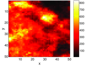
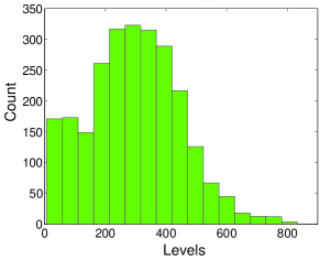
We investigate the application of the spin-based models on real-world data. We compare the results with the KNN, FKNN, and Support Vector Machine (SVM) methods. We consider remotely sensed rainfall data on a moderately sized $50\times 50$ grid. The study domain covers an area of Indonesia extending from 2.5S to 10N in latitude and from 110E to 122.5E in longitude, covered with a resolution of $0.25^{\circ}\times 0.25^{\circ}$. A map of the precipitation distribution is shown in Fig. 7(a). The data represent daily accumulated rainfall values recorded during January 2007 (http://disc2.nascom.nasa.gov/Giovanni/tovas/TRMM_V6.3B42_daily.shtml) giovanni . The values are in millimeters and some summary statistics are as follows: $z_{\min}=7.1$, $z_{\max}=832.6$, $\bar{z}=295.0$, $z_{0.50}=293.7$, $\sigma_{z}=151.4$. The skewness coefficient is $0.27$ and the kurtosis coefficient $2.93$. As evidenced in the histogram shown in Fig. 7(b), the precipitation p.d.f. is non-Gaussian, possibly bimodal.

(a) Map

(b) Histogram

Figure 7: (Color online) Map and histogram of precipitation values for the complete rainfall data.

The KNN and FKNN results are obtained with an optimally tuned parameter $k_{\rm opt}$ for each realization. In the case of SVM, two hyperparameters, $C$ and $\sigma_{k}$, need to be tuned for each of the $N_{c}$ binary classifiers. For different values of $C$, we found the bandwidth value $\sigma_{\rm kopt}$ that minimizes globally the “testing errors” for each of the $N_{c}$ classifiers (the true values at all the prediction points were used for testing). We selected a $C_{\rm opt}$ that minimizes the testing error. The obtained misclassification rates were relatively high in this class-adaptive approach, and further fine-tuning of the hyperparameters did not bring noticeable improvements. Better results were obtained by using mean values of $\sigma_{\rm kopt}$ and $C_{\rm opt}$, for all $N_{c}$ classifiers. Using the same values of the hyperparameters for all the $N_{c}$ classifiers has been shown to give satisfactory results kane02 . Furthermore, we used the same hyperparameters for the ten realizations, since they were all derived from a uniform thinning of the same rainfall data set.

Table 8: Average misclassification rates for the $N_{c}$-level INNC, PNNC, and CNNC models. The averages are calculated over $10$ randomly thinned (by $p\,\%$) samples of the rainfall data. These are compared with the best (lowest values) obtained using the KNN and SVM techniques. The following misclassification rates are used: $\langle F^{*}_{I}\rangle$ for the INNC, $\langle F^{*}_{P}\rangle$ for the PNNC, $\langle F^{*}_{C}\rangle$ for the CNNC, $\langle F^{*}_{\rm knn}\rangle$ for the KNN, $\langle F^{*}_{\rm fknn}\rangle$ for the FKNN, and $\langle F^{*}_{\rm SVM}\rangle$ for the SVM.

# of classes	$N_{c}=2$		$N_{c}=4$		$N_{c}=8$		$N_{c}=16$
$p[\%]$	$33$	$66$	$33$	$66$	$33$	$66$	$33$	$66$
$\langle F^{*}_{I}\rangle$	6.81	8.61	13.41	16.94	24.51	30.46	44.95	53.05
$\langle F^{*}_{P}\rangle$	6.51	8.43	14.18	17.53	27.87	33.01	51.59	56.25
$\langle F^{*}_{C}\rangle$	6.86	8.62	14.68	17.84	28.63	32.97	50.32	55.28
$\langle F^{*}_{\rm knn}\rangle$	6.46	8.47	13.82	18.01	28.28	33.85	51.85	56.12
$\langle F^{*}_{\rm fknn}\rangle$	6.12	7.91	12.99	16.72	26.55	31.63	49.67	54.08
$\langle F^{*}_{\rm SVM}\rangle$	6.78	8.56	15.61	17.62	29.70	33.61	51.27	55.49

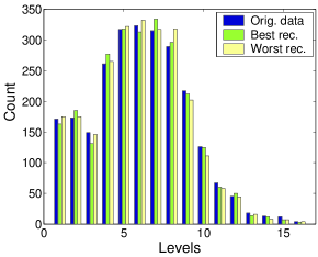
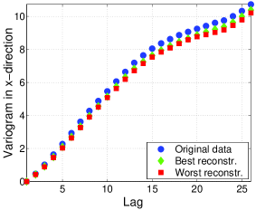
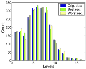
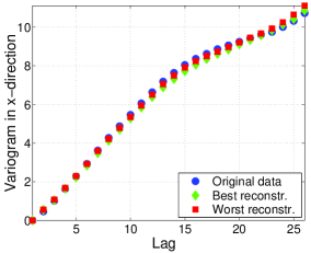
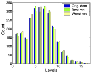
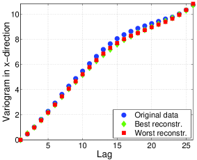
In Table 8 we compare average misclassification rates for the spin-based models, as well as the KNN, FKNN, and SVM classifiers based on 10 different sampling realizations. The sample sets are derived from random thinning of the rainfall data by $p\,\%.$ Comparing the performance of different classifiers, the FKNN and the INNC models give the best results overall. FKKN performs better for small number of classes $(N_{c}=2,4),$ while INNC is better at larger values of $N_{c}$. These results agree with the synthetic data studies, where the INNC model also showed superior performance, especially for the data with slower variation and moderate degree of thinning. In contrast to the synthetic studies, the CNNC model did not perform as satisfactorily. This could be attributed to the presence of noise (ubiquitous in real data), as pointed out in Section IV. In addition, the SVM classifier did not perform as well as in some other comparative studies herm99 ; shari03 ; mull97 . This may be due to the simplifications we adopted in the estimation of the hyperparameters. Besides the misclassification rates, we also checked the capacity of the respective classifiers to reproduce the histogram and the empirical directional variogram, $\hat{\gamma}_{Z}(r{\bf e})$ of the data yagl87 . The $\hat{\gamma}_{Z}(r{\bf e})$, also known as the two-point structure function, is a measure of the spatial continuity of the field $Z$ in the direction ${\bf e}=\hat{\bf x}$. On a lattice of step $\alpha$, the $\hat{\gamma}_{Z}(r{\bf e})$ is given by

$$\hat{\gamma}_{Z}(n\alpha\hat{\bf x})=\frac{1}{2\,L(L-n)}\sum_{j=1}^{L-n}\sum_{i=1}^{L}\left[Z({\bf s}_{i,j+n})-Z({\bf s}_{i,j})\right]^{2},\;r=n\alpha,\;n=1,\ldots,\frac{L}{2},$$ (10)

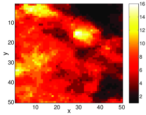
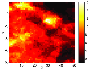
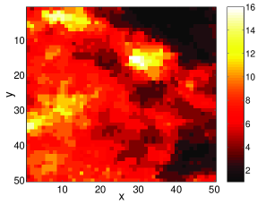
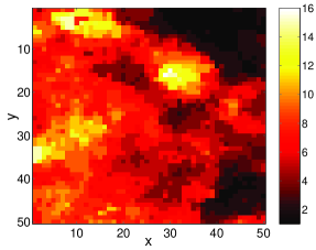
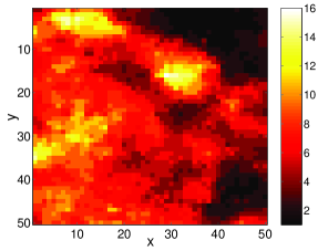
where ${\bf s}_{i,j}=\alpha\,(i\hat{\bf y}+j\hat{\bf x}).$ In Figs. 8-10, we show the reconstructed maps, histograms, and variograms in the direction of the $x$ axis, for the best (lowest $F^{*}$) and worst (highest $F^{*}$) reconstructed realizations for $N_{c}=16$ and $p=0.33$, based on 100 realizations. The variogram along the $y$ axis (not shown) has similar behavior. In all the cases, the statistics are recovered satisfactorily, and there are no significant differences between the respective models. Even though the PNNC model gave the highest misclassification rate, it reproduces the histograms and the variogram reasonably well.

(a) Best map by INNC

(b) Worst map by INNC

(c) Histograms by INNC

(d) x-variogram by INNC

Figure 8: (Color online) 16-class classification results of the rainfall data with $p=33\%$ missing values obtained by the INNC model. Using $100$ reconstructions derived from different sampling configurations, we show the class maps of the best (a) and worst (b) case reconstructions, the class histograms of the original data as well as the best and worst reconstructions (c), and the empirical class variogram in the horizontal direction (d) for the original data as well as the best and worst reconstructions.

(a) Best map by PNNC

(b) Worst map by PNNC

(c) Histograms by PNNC

(d) x-variogram by PNNC

Figure 9: (Color online) 16-class classification results of the rainfall data obtained by the PNNC model. The plot captions correspond to those in Fig. 8.

(a) Best map by CNNC

(b) Worst map by CNNC

(c) Histograms by CNNC

(d) x-variogram by CNNC

Figure 10: (Color online) 16-class classification results of the rainfall data obtained by the CNNC model. The plot captions correspond to those in Fig. 8.

The above simulation results are based on one run for each sample set. As we have shown in the case of synthetic data, multiple runs can improve the results and allow estimation of uncertainty. In the case of the rainfall data, considering one realization (sample set) generated with $p=0.33$ and performing 100 simulation runs using, for example, the 16-level CNNC model gave the misclassification rate $F^{*}=46.9\%$ requiring $T_{\rm cpu}=5.6$ seconds of total CPU time. The multiple-run-reconstruction measures, as those shown in Fig. 6 for the synthetic data, are displayed in Fig. 11.

(a) Original

(b) Sample

(c) Reconstructed

(d) Histograms

(e) Conf. interval

(f) RMSE

Figure 11: (Color online) Classification results obtained from the 16-class CNNC model. The missing-values sample is obtained from the rainfall data by randomly removing $p=0.33$ of the points. One hundred reconstructions are generated starting from 100 initial states obtained by the majority rule with adaptable stencil size. Plots (a)-(c) show class maps for the complete realization, the sample with the missing data, and the reconstructed image, respectively. The latter is based on the medians of the class values obtained from the 100 reconstructions. Plot (d) compares the class histograms of the original and reconstructed data, plot (e) shows the width of the $95\%$ confidence intervals for the class predictions, and plot (f) represents the class root mean square error at the prediction points.

V.2 Digital image data

We consider the standard 256-valued gray-scale test image of Lena on a $512\times 512$ grid. We randomly remove $p=33\%$ of the pixels and subsequently reconstruct the image using the spin-based models. The degraded image is shown in Fig. 12.

Figure 12: Degraded image of Lena obtained by random removal of $33\%$ of the pixels.

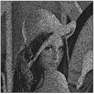
The range of the image pixel values is equal to $\max(Z)-\min(Z)=220$, and thus we use $N_{c}=220$ classes of uniform width (equal to 1). The sequence in Fig. 13 shows the original image, Fig. 13(a), along with the reconstructed images obtained by the INNC, Fig. 13(b), PNNC, Fig. 13(c), and CNNC, Fig. 13(d) models. Visually, all three reconstructions appear quite similar to the original image. The INNC model misclassifies some pixels along the edges (e.g., along the shoulder). The numerical comparisons of univariate validation measures shown in Table 9 are in favor of the CNNC model. The CNNC model is also more efficient computationally (requiring fewer MC sweeps and less CPU time), and it also approximates more accurately the sample energy. The worst performance in terms of the validation measures is shown by the PNNC model.

(a) Original

(b) INNC

(c) PNNC

(d) CNNC

Figure 13: Original (a) and reconstructed images of Lena using the INNC (b), PNNC (c) and CNNC (d) classification models.

Table 9: Prediction errors and average optimization statistics for reconstructions of the Lena image by means of the INNC, PNNC, and CNNC models, based on $10$ realizations corresponding to different sampling configurations. MAAE: Mean average absolute error. MARE: Mean average relative error. MAARE: Mean average absolute relative error. MRASE: Mean root average square error. MR: Mean Correlation coefficient. First, averages are evaluated over the prediction points for each realization, and then means are calculated with respect to an ensemble of $10$ realizations.

	MAAE	MARE [%]	MAARE [%]	MRASE	MR [%]	$\langle N_{MC}\rangle$	$\langle T_{\rm cpu}\rangle$ [s]	$\langle U^{*}\rangle$
INNC	5.04	2.63	4.97	9.29	98.35	106.9	351.1	3e-4
PNNC	6.20	0.21	6.48	11.67	97.08	571.4	275.7	0.14
CNNC	5.04	-3e-6	5.33	8.24	98.52	8.3	173.7	2e-10

VI Summary and conclusions

We present spatial classification methods for missing data on partially sampled Cartesian grids, based on non-parametric spin models from statistical physics (e.g., Ising, Potts, clock and XY models). The methods are based on the idea of matching the normalized correlation energy of the sampled spins with that of the entire grid. The matching is performed using greedy Monte Carlo simulation conditioned by the sample values. The non-parametric spin-based classifiers presented here embody isotropic nearest-neighbor correlations. Hence, they are expected to perform well if the data exhibit a degree of spatial continuity and structure dominated by local features. Many geophysical and remotely sensed data as well as digital images share these features. The models presented here are not in principle suitable for capturing long-range correlations, such as those characterizing the transport properties of geological media. Nonetheless, it should be pointed out that the spatial features of the “reconstructed” field are not determined exclusively by the properties of the classification model but also by the features (e.g., anisotropic correlations) present in the sample.

The relative performance of the spin models in the case studies investigated varied, depending on the type of data, the sampling density, and the number of classes considered. Overall, the INNC model, which is based on a sequential classification algorithm, gave the most accurate classification rates in most of the cases studied. For all the simulated data, the PNNC model gave the highest misclassification rates. We believe that this is mainly due to the higher spatial degeneracy of the PNNC model. For noise-free data with short-range differentiable variations, the CNNC model that incorporates cross-class correlations performed best, especially for the higher class numbers. As the number of classes increases, the CNNC model tends to the continuous XY model, and the classification emulates spatial interpolation. Up to a threshold, increasing the number of classes gradually lowers spatial prediction errors at the cost of a moderate increase in computing time. The classification performance of the spin-based methods can be further improved by executing multiple runs starting from different initial states. This strategy also permits an estimate of the classification uncertainty. The classification performance of the spin-based models was compared with the $k$-nearest neighbor (KNN), and the fuzzy $k$-nearest neighbor (FKNN) algorithms, and (for the rainfall data) with the Support Vector Machine (SVM) classifier. For the synthetic data the INNC and CNNC models gave uniformly lower misclassification rates than the KNN and FKNN algorithms. For classification of real data into a small number of classes, the FKNN algorithm with optimized $k$ was the most accurate of the classifiers tested.

All the spin-based models are computationally efficient. For the PNNC, CNNC, and XYNNC models, the mean CPU time ranged from $0.03$ seconds (PNNC model, $L=50$, $p=0.33$, $N_{c}=8$) to $5$ seconds (CNNC model, $L=200$, $p=0.66$, and $N_{c}=16$). For the INNC model, the CPU time is generally higher due to the cost of determining the initial state at each level. In contrast, the time needed for the Monte Carlo relaxation is very short. Therefore, the resulting INNC CPU time varies almost linearly with the number of classes, and in our study it ranged from $0.08$ to almost $14$ seconds. We do not report CPU times for the KNN, FKNN, and SVM computations, since in order to optimize the classification accuracy significant computational time was devoted to fine-tuning the hyperparameters.

An advantage of the spin-based models with respect to the other classifiers tested is the lack of hyperparameters that need tuning by the user. Hence the classification procedure can be automated, and it provides competitive accuracy as well as computational efficiency. Compared to linear spatial interpolation algorithms (e.g., kriging), the spin-based classification methods present the advantages of computational efficiency and ability to handle non-Gaussian probability distributions at the expense of introducing discrete intervals in place of continuous values. A comparative study of the two approaches in the future could help to quantify their relative merits.

Currently, the spin-based models are formulated on a regular grid. Hence, potential areas of application involve the compression of large images and the reconstruction of missing values (e.g., image pixels). Note that in light of the comments in Section III, the energy matching principle is not suitable for the refinement (resampling) of a regular grid, e.g., by doubling the spatial resolution. Extension to irregular sampling patterns is possible by defining a distance-dependent interaction strength $J_{i,j}=J_{0}\,K(\vec{r}_{ij})$, where $J_{0}$ is arbitrary and $K(\vec{r}_{ij})$ is a normalized function of $\vec{r}_{ij}$, over a specified interaction neighborhood. Other potential extensions include extended-range interactions and/or “multi-point spin” correlations in the respective Hamiltonians. This could also help to eliminate the spatial degeneracy evident in the present models, and provide more flexible measures of spatial dependence at the expense of concomitant increases in computational time and parametrization.