A Comparison of Bimolecular Reaction Models for Stochastic Reaction Diffusion Systems

I. C. Agbanusi   and S. A. Isaacson Department of Mathematics and Statistics, Boston University, 111 Cummington St., Boston, MA 02215 (agbanusi@math.bu.edu) Department of Mathematics and Statistics, Boston University, 111 Cummington St., Boston, MA 02215 (isaacson@math.bu.edu)
Abstract

Stochastic reaction-diffusion models have become an important tool in studying how both noise in the chemical reaction process and the spatial movement of molecules influences the behavior of biological systems. There are two primary spatially-continuous models that have been used in recent studies; the diffusion limited reaction model of Smoluchowski, and a second approach popularized by Doi. Both models treat molecules as points undergoing Brownian motion. The former represents chemical reactions between two reactants through the use of reactive boundary conditions, with two molecules reacting instantly upon reaching a fixed separation (called the reaction-radius). The Doi model uses reaction potentials, whereby two molecules react with a fixed probability per unit time, λ𝜆\lambda, when separated by less than the reaction radius. In this work we study the rigorous relationship between the two models. For the special case of a protein diffusing to a fixed DNA binding site, we prove that the solution to the Doi model converges to the solution of the Smoluchowski model as λ𝜆\lambda\to\infty, with a rigorous O(λ12+ϵ)𝑂superscript𝜆12italic-ϵO(\lambda^{-\frac{1}{2}+\epsilon}) error bound (for any fixed ϵ>0italic-ϵ0\epsilon>0). We investigate by numerical simulation, for biologically relevant parameter values, the difference between the solutions and associated reaction time statistics of the two models. As the reaction-radius is decreased, for sufficiently large but fixed values of λ𝜆\lambda, these differences are found to increase like the inverse of the binding radius.

1 Introduction

Stochastic reaction-diffusion models have become a popular tool for modeling biological systems in which both noise in the chemical reaction process and the spatial diffusion of molecules play an important roll. Such models have been used in a multitude of recent studies, examining the dynamics of synaptic transmission [33]; the MinCDE system in bacteria [10]; how proteins search for DNA binding sites [26]; and studies of signaling in the cell membrane [9]. There are three primary stochastic reaction-diffusion models that these studies have made use of; the diffusion limited reaction model of Smoluchowski [35, 28], what we call the Doi model [38, 5, 6], and the reaction diffusion master equation (RDME) [16, 12, 27].

In the Doi and Smoluchowski models, the positions of molecules are represented as points undergoing Brownian motion. Bimolecular reactions between two molecules in the Doi model occur with a fixed probability per unit time when two reactants are separated by less than some specified “reaction radius”. The Smoluchowski model differs by representing bimolecular reactions in one of two ways; either occurring instantaneously, or with fixed probability per unit time, when two reactants’ separation is exactly the reaction-radius [35, 28]. In this work we focus on the former case (often called a pure absorption reaction). For both models unimolecular reactions represent internal processes. They are assumed to occur with exponentially distributed times based on a specified reaction-rate constant. For general chemical systems, both the Doi and Smoluchowski models can be described by, possibly infinite, systems of partial integral differential equations (PIDEs) for the probability densities of having a given number of each chemical species and the corresponding locations of each molecule.

The RDME is spatially discrete, and given by a, possibly infinite, system of ODEs for the numbers of each chemical species located at each lattice site. It can be interpreted as an extension of the non-spatial chemical master equation (CME) [16, 32, 15, 39] model for stochastic chemical kinetics. Formally, the RDME has been shown to be an approximation to both the Doi model [22] and the Smoluchowski model [23, 25, 13, 20] for appropriately chosen lattice spacings. These approximations break down for systems involving bimolecular reactions, in two or more dimensions, in the limit that the lattice spacing approaches zero [23, 20]. (Recently we have suggested a new convergent RDME (CRDME) that converges to the Doi model as the lattice spacing is taken to zero [24].)

There are a plethora of numerical methods and simulation packages that have been developed to study biological systems based on one of the Smoluchowski, Doi, or RDME models. These include the λ𝜆\lambda-ρ𝜌\rho method [11, 31], the CRDME [24], the FPKMC [7, 36], MCELL [29], MesoRD [14], Smoldyn [1], STEPS [21], and URDME [8]. While these numerical methods and software packages have been used in many modeling efforts, it is still an open question how exactly the underlying mathematical models they approximate are rigorously related. Moreover, to compare the results of modeling studies it would be helpful to understand how to choose parameters in the Doi (resp. Smoluchowski) model to accurately approximate the Smoluchowski (resp. Doi) model.

To address these questions, we investigate the rigorous relationship between the Doi and (pure absorption) Smoluchowski models. We begin in the next section by giving a brief overview of the general Doi and Smoluchowski models for the bimolecular reaction A+BCABC\textrm{A}+\textrm{B}\to\textrm{C}. (The two models are identical for systems with only first or zeroth order reactions.) We then consider the special case of a single protein searching for a DNA binding site within the nucleus of a eukaryotic cell in Section 3. The binding site is located at the origin, and the nucleus is modeled as a concentric sphere of radius R𝑅R. With the further assumption that the initial distribution of the protein’s position is rotationally invariant, the Doi and Smoluchowski models can be simplified to spherically-symmetric diffusion equations. For the Doi model the diffusing protein is allowed to bind with probability per unit time λ𝜆\lambda when within a reaction-radius, rbsubscript𝑟br_{\textrm{b}}, of the binding site. This leads to a “reaction potential” in the PDE for the Doi model. In the Smoluchowski model the protein reacts instantly upon reaching a separation rbsubscript𝑟br_{\textrm{b}} from the binding site. This leads to the replacement of the reaction potential with a zero Dirichlet boundary condition on the sphere of radius rbsubscript𝑟br_{\textrm{b}} around the origin.

Denote by pλ(r,t)subscript𝑝𝜆𝑟𝑡p_{\lambda}(r,t) the spherically symmetric probability density that the diffusing molecule is r𝑟r from the origin at time t𝑡t in the Doi model, and by ρ(r,t)𝜌𝑟𝑡\rho(r,t) the corresponding probability density in the Smoluchowski model. In Section 4 we numerically calculate the difference between pλ(r,t)subscript𝑝𝜆𝑟𝑡p_{\lambda}(r,t) and ρ(r,t)𝜌𝑟𝑡\rho(r,t) for biologically relevant parameter values. We find that pλ(r,t)ρ(r,t)subscript𝑝𝜆𝑟𝑡𝜌𝑟𝑡p_{\lambda}(r,t)\to\rho(r,t) uniformly in r𝑟r and t𝑡t as λ𝜆\lambda\to\infty, with an empirical convergence rate that is O(λ12)𝑂superscript𝜆12O(\lambda^{-\frac{1}{2}}). The same empirical convergence rate is observed for the corresponding binding time distributions and mean binding times of the two models. For sufficiently large, but fixed, values of λ𝜆\lambda, as rbsubscript𝑟br_{\textrm{b}} is decreased the difference between the probability densities, binding time distributions, and mean binding times increase like rb1superscriptsubscript𝑟b1r_{\textrm{b}}^{-1}.

These results motivate our studies in Section 5, where we rigorously prove the convergence of pλ(r,t)subscript𝑝𝜆𝑟𝑡p_{\lambda}(r,t) to ρ(r,t)𝜌𝑟𝑡\rho(r,t) as λ𝜆\lambda\to\infty with an O(λ12+ϵ)𝑂superscript𝜆12italic-ϵO(\lambda^{-\frac{1}{2}+\epsilon}) error bound (for all ϵ>0italic-ϵ0\epsilon>0). Let μnsubscript𝜇𝑛\mu_{n} denote the n𝑛nth eigenvalue of the generator of the Doi model (see (15)), with αnsubscript𝛼𝑛\alpha_{n} the n𝑛nth eigenvalue of the generator of the Smoluchowski model (see (11)). Our approach is to first prove that for λ𝜆\lambda sufficiently large, if αnM(λ)subscript𝛼𝑛𝑀𝜆\alpha_{n}\leq M(\lambda) with M(λ)𝑀𝜆M(\lambda) a specified increasing function of λ𝜆\lambda, then

|αnμn|Cλ12ϵsubscript𝛼𝑛subscript𝜇𝑛𝐶superscript𝜆12italic-ϵ\left|\alpha_{n}-\mu_{n}\right|\leq\frac{C}{\lambda^{\frac{1}{2}-\epsilon}}

for any fixed ϵ>0italic-ϵ0\epsilon>0. The precise statement of this result is given in Theorem 5.1. This theorem is then used to show the corresponding eigenfunction convergence result in Lemma 5.1. Denote by ψn(r)subscript𝜓𝑛𝑟\psi_{n}(r) the n𝑛nth eigenfunction of the generator of the Doi model (15), and ϕn(r)subscriptitalic-ϕ𝑛𝑟\phi_{n}(r) the corresponding eigenfunction of the Smoluchowski model (11). We prove for λ𝜆\lambda sufficiently large and μn<M(λ)subscript𝜇𝑛𝑀𝜆\mu_{n}<M(\lambda) that

supr[rb,R]|ϕn(r)ψn(r)|Cλ12ϵ.subscriptsupremum𝑟subscript𝑟b𝑅subscriptitalic-ϕ𝑛𝑟subscript𝜓𝑛𝑟𝐶superscript𝜆12italic-ϵ\sup_{r\in\left[r_{\textrm{b}},R\right]}\left|\phi_{n}(r)-\psi_{n}(r)\right|\leq\frac{C}{\lambda^{\frac{1}{2}-\epsilon}}.

Finally, the preceding two results are used to prove that

supt(δ,)supr(rb,R)|pλ(r,t)ρ(r,t)|Cλ12ϵ,subscriptsupremum𝑡𝛿subscriptsupremum𝑟subscript𝑟b𝑅subscript𝑝𝜆𝑟𝑡𝜌𝑟𝑡𝐶superscript𝜆12italic-ϵ\sup_{t\in\left(\delta,\infty\right)}\sup_{r\in\left(r_{\textrm{b}},R\right)}\left|p_{\lambda}(r,t)-\rho(r,t)\right|\leq\frac{C}{\lambda^{\frac{1}{2}-\epsilon}}, (1)

for any ϵ>0italic-ϵ0\epsilon>0 and δ>0𝛿0\delta>0 fixed. The precise statement of this result is given in Theorem 5.2.

It should be noted that the approximation of Dirichlet boundary conditions by reaction potentials is a well-studied problem in the context of the large-coupling limit in quantum physics [19]. Our approach of proving convergence through successive eigenvalue, eigenfunction, and PDE solution estimates differs from the more standard resolvent and path integral estimates [37, 3, 2]. A similar convergence rate of the Doi model solution to the Smoluchowski model solution was proven in L2(3)superscript𝐿2superscript3L^{2}(\mathbb{R}^{3}) in [4] (as opposed to the uniform convergence rate (1) we prove in a spherical domain). Denote by 𝟏[0,rb](r)subscript10subscript𝑟b𝑟\mathbf{1}_{\left[0,r_{\textrm{b}}\right]}(r) the indicator function of the interval, [0,rb]0subscript𝑟b\left[0,r_{\textrm{b}}\right]. Convergence rates for eigenvalues of the general one-dimensional operator d2dx2+V(x)+λW(x)superscript𝑑2𝑑superscript𝑥2𝑉𝑥𝜆𝑊𝑥-\frac{d^{2}{}}{d{x}^{2}}+V(x)+\lambda W(x) as λ𝜆\lambda\to\infty, for x𝑥x\in\mathbb{R}, were proven in [17]. In contrast, in Section 5 we study the spherically symmetric operator arising in the Doi model, d2dr22rddr+λ𝟏[0,rb](r)superscript𝑑2𝑑superscript𝑟22𝑟𝑑𝑑𝑟𝜆subscript10subscript𝑟b𝑟-\frac{d^{2}{}}{d{r}^{2}}-\frac{2}{r}\frac{d}{dr}+\lambda\mathbf{1}_{\left[0,r_{\textrm{b}}\right]}(r) for r[0,R)𝑟0𝑅r\in\left[0,R\right) with a Neumann boundary condition at R𝑅R, directly.

2 General Doi and Smoluchowski Models

We first illustrate how the bimolecular reaction A+BCABC\textrm{A}+\textrm{B}\to\textrm{C} would be described by the Doi and Smoluchowski models in 3superscript3\mathbb{R}^{3}. In the Doi model, bimolecular reactions are characterized by two parameters; the separation at which molecules may begin to react, rbsubscript𝑟br_{\textrm{b}}, and the probability per unit time the molecules react when within this separation, λ𝜆\lambda. In the Doi and Smoluchowski models, when a molecule of species A and a molecule of species B react we assume the C molecule they produce is placed midway between them.

We now formulate the Doi model as an infinite coupled system of PIDEs. Let 𝒒la3subscriptsuperscript𝒒𝑎𝑙superscript3\boldsymbol{q}^{a}_{l}\in\mathbb{R}^{3} denote the position of the l𝑙lth molecule of species A when the total number of molecules of species A is a𝑎a. The state vector of the species A molecules is then given by 𝒒a=(𝒒1a,,𝒒aa)3asuperscript𝒒𝑎subscriptsuperscript𝒒𝑎1subscriptsuperscript𝒒𝑎𝑎superscript3𝑎\boldsymbol{q}^{a}=(\boldsymbol{q}^{a}_{1},\dots,\boldsymbol{q}^{a}_{a})\in\mathbb{R}^{3a}. Define 𝒒bsuperscript𝒒𝑏\boldsymbol{q}^{b} and 𝒒csuperscript𝒒𝑐\boldsymbol{q}^{c} similarly. We denote by f(a,b,c)(𝒒a,𝒒b,𝒒c,t)superscript𝑓𝑎𝑏𝑐superscript𝒒𝑎superscript𝒒𝑏superscript𝒒𝑐𝑡f^{(a,b,c)}(\boldsymbol{q}^{a},\boldsymbol{q}^{b},\boldsymbol{q}^{c},t) the probability density for there to be a𝑎a molecules of species A, b𝑏b molecules of species B, and c𝑐c molecules of species C at time t𝑡t located at the positions 𝒒asuperscript𝒒𝑎\boldsymbol{q}^{a}, 𝒒bsuperscript𝒒𝑏\boldsymbol{q}^{b}, and 𝒒csuperscript𝒒𝑐\boldsymbol{q}^{c}. Molecules of the same species are assumed indistinguishable. In the Doi model the evolution of f(a,b,c)superscript𝑓𝑎𝑏𝑐f^{(a,b,c)} is given by

f(a,b,c)t(𝒒a,𝒒b,𝒒c,t)=(L+R)f(a,b,c)(𝒒a,𝒒b,𝒒c,t).superscript𝑓𝑎𝑏𝑐𝑡superscript𝒒𝑎superscript𝒒𝑏superscript𝒒𝑐𝑡𝐿𝑅superscript𝑓𝑎𝑏𝑐superscript𝒒𝑎superscript𝒒𝑏superscript𝒒𝑐𝑡\frac{\partial f^{(a,b,c)}}{\partial t}\left(\boldsymbol{q}^{a},\boldsymbol{q}^{b},\boldsymbol{q}^{c},t\right)=\left(L+R\right)f^{(a,b,c)}\left(\boldsymbol{q}^{a},\boldsymbol{q}^{b},\boldsymbol{q}^{c},t\right). (2)

Note, with the subsequent definitions of the operators L𝐿L and R𝑅R this will give a coupled system of PIDEs over all possible values of (a,b,c)𝑎𝑏𝑐(a,b,c). More general systems that allow unbounded production of certain species would result in an infinite number of coupled PIDEs. The diffusion operator, L𝐿L, is defined by

Lf(a,b,c)(𝒒a,𝒒b,𝒒c,t)𝐿superscript𝑓𝑎𝑏𝑐superscript𝒒𝑎superscript𝒒𝑏superscript𝒒𝑐𝑡\displaystyle Lf^{(a,b,c)}\left(\boldsymbol{q}^{a},\boldsymbol{q}^{b},\boldsymbol{q}^{c},t\right) =(DAl=1aΔla+DBm=1bΔmb+DCn=1cΔnc)f(a,b,c)(𝒒a,𝒒b,𝒒c,t),absentsuperscript𝐷Asuperscriptsubscript𝑙1𝑎superscriptsubscriptΔ𝑙𝑎superscript𝐷Bsuperscriptsubscript𝑚1𝑏superscriptsubscriptΔ𝑚𝑏superscript𝐷Csuperscriptsubscript𝑛1𝑐superscriptsubscriptΔ𝑛𝑐superscript𝑓𝑎𝑏𝑐superscript𝒒𝑎superscript𝒒𝑏superscript𝒒𝑐𝑡\displaystyle=\left(D^{\textrm{A}}\sum_{l=1}^{a}\Delta_{l}^{a}+D^{\textrm{B}}\sum_{m=1}^{b}\Delta_{m}^{b}+D^{\textrm{C}}\sum_{n=1}^{c}\Delta_{n}^{c}\right)f^{(a,b,c)}\left(\boldsymbol{q}^{a},\boldsymbol{q}^{b},\boldsymbol{q}^{c},t\right), (3)

where ΔlasuperscriptsubscriptΔ𝑙𝑎\Delta_{l}^{a} denotes the Laplacian in the coordinate 𝒒lasubscriptsuperscript𝒒𝑎𝑙\boldsymbol{q}^{a}_{l} and DAsuperscript𝐷AD^{\textrm{A}} the diffusion constant of species A. DBsuperscript𝐷BD^{\textrm{B}}, DCsuperscript𝐷CD^{\textrm{C}}, ΔmbsuperscriptsubscriptΔ𝑚𝑏\Delta_{m}^{b}, and ΔncsuperscriptsubscriptΔ𝑛𝑐\Delta_{n}^{c} are defined similarly.

To define the reaction operator, R𝑅R, we must introduce notations to represent removing or adding a specific molecule to the state 𝒒asuperscript𝒒𝑎\boldsymbol{q}^{a}. Let

𝒒a𝒒la=(𝒒1a,,𝒒l1a,𝒒l+1a,,𝒒aa),superscript𝒒𝑎subscriptsuperscript𝒒𝑎𝑙subscriptsuperscript𝒒𝑎1subscriptsuperscript𝒒𝑎𝑙1subscriptsuperscript𝒒𝑎𝑙1subscriptsuperscript𝒒𝑎𝑎\displaystyle\boldsymbol{q}^{a}\setminus\boldsymbol{q}^{a}_{l}=\left(\boldsymbol{q}^{a}_{1},\dots,\boldsymbol{q}^{a}_{l-1},\boldsymbol{q}^{a}_{l+1},\dots,\boldsymbol{q}^{a}_{a}\right), 𝒒a𝒒=(𝒒1a,,𝒒aa,𝒒).superscript𝒒𝑎𝒒subscriptsuperscript𝒒𝑎1subscriptsuperscript𝒒𝑎𝑎𝒒\displaystyle\boldsymbol{q}^{a}\cup\boldsymbol{q}=\left(\boldsymbol{q}^{a}_{1},\dots,\boldsymbol{q}^{a}_{a},\boldsymbol{q}\right).

𝒒a𝒒superscript𝒒𝑎𝒒\boldsymbol{q}^{a}\setminus\boldsymbol{q} will denote 𝒒asuperscript𝒒𝑎\boldsymbol{q}^{a} with any one component with the value 𝒒𝒒\boldsymbol{q} removed. Denote by 𝟏[rrb](r)subscript1delimited-[]𝑟subscript𝑟b𝑟\mathbf{1}_{\left[r\leq r_{\textrm{b}}\right]}(r) the indicator function of the interval [0,rb]0subscript𝑟b\left[0,r_{\textrm{b}}\right], and let Blc={𝒒3||𝒒𝒒lc|rb/2}superscriptsubscript𝐵𝑙𝑐conditional-set𝒒superscript3𝒒subscriptsuperscript𝒒𝑐𝑙subscript𝑟b2B_{l}^{c}=\{\boldsymbol{q}\in\mathbb{R}^{3}|\left|\boldsymbol{q}-\boldsymbol{q}^{c}_{l}\right|\leq r_{\textrm{b}}/2\} label the set of points a reactant could be at to produce a molecule of species C at 𝒒lcsubscriptsuperscript𝒒𝑐𝑙\boldsymbol{q}^{c}_{l}. The Doi reaction operator, R𝑅R, is then

(Rf(a,b,c))(𝒒a,𝒒b,𝒒c,t)=λ[l=1c𝒒BlCf(a+1,b+1,c1)(𝒒a𝒒,𝒒b(2𝒒lc𝒒),𝒒c𝒒lc,t)dBlcl=1al=1b𝟏[0,rb](|𝒒la𝒒lb|)f(a,b,c)(𝒒a,𝒒b,𝒒c,t)].𝑅superscript𝑓𝑎𝑏𝑐superscript𝒒𝑎superscript𝒒𝑏superscript𝒒𝑐𝑡𝜆delimited-[]superscriptsubscript𝑙1𝑐subscript𝒒superscriptsubscript𝐵𝑙𝐶superscript𝑓𝑎1𝑏1𝑐1superscript𝒒𝑎𝒒superscript𝒒𝑏2subscriptsuperscript𝒒𝑐𝑙𝒒superscript𝒒𝑐subscriptsuperscript𝒒𝑐𝑙𝑡𝑑superscriptsubscript𝐵𝑙𝑐superscriptsubscript𝑙1𝑎superscriptsubscriptsuperscript𝑙1𝑏subscript10subscript𝑟bsubscriptsuperscript𝒒𝑎𝑙subscriptsuperscript𝒒𝑏superscript𝑙superscript𝑓𝑎𝑏𝑐superscript𝒒𝑎superscript𝒒𝑏superscript𝒒𝑐𝑡(Rf^{(a,b,c)})\left(\boldsymbol{q}^{a},\boldsymbol{q}^{b},\boldsymbol{q}^{c},t\right)=\lambda\Bigg{[}\sum_{l=1}^{c}\int_{\boldsymbol{q}\in B_{l}^{C}}f^{(a+1,b+1,c-1)}\left(\boldsymbol{q}^{a}\cup\boldsymbol{q},\boldsymbol{q}^{b}\cup\left(2\boldsymbol{q}^{c}_{l}-\boldsymbol{q}\right),\boldsymbol{q}^{c}\setminus\boldsymbol{q}^{c}_{l},t\right)\,dB_{l}^{c}\\ -\sum_{l=1}^{a}\sum_{l^{\prime}=1}^{b}\mathbf{1}_{\left[0,r_{\textrm{b}}\right]}\big{(}\big{|}\boldsymbol{q}^{a}_{l}-\boldsymbol{q}^{b}_{l^{\prime}}\big{|}\big{)}f^{(a,b,c)}(\boldsymbol{q}^{a},\boldsymbol{q}^{b},\boldsymbol{q}^{c},t)\Bigg{]}. (4)

In the Fock space representation of [5, 6], the term Rf(a,b,c)𝑅superscript𝑓𝑎𝑏𝑐Rf^{(a,b,c)} is called a reaction potential [6].

The Smoluchowski model would modify (2) by adding a reactive boundary condition and changing the reaction operator (4). The reactive boundary condition, often called a “pure absorption” boundary condition, is the Dirichlet boundary condition that

f(a,b,c)(𝒒a,𝒒b,𝒒c,t)=0,if |𝒒la𝒒mb|=rb, for any l,m.formulae-sequencesuperscript𝑓𝑎𝑏𝑐superscript𝒒𝑎superscript𝒒𝑏superscript𝒒𝑐𝑡0if subscriptsuperscript𝒒𝑎𝑙subscriptsuperscript𝒒𝑏𝑚subscript𝑟b for any 𝑙𝑚f^{(a,b,c)}\left(\boldsymbol{q}^{a},\boldsymbol{q}^{b},\boldsymbol{q}^{c},t\right)=0,\quad\text{if }\left|\boldsymbol{q}^{a}_{l}-\boldsymbol{q}^{b}_{m}\right|=r_{\textrm{b}},\text{ for any }l,m. (5)

We define by Slc={𝒒3||𝒒𝒒lc|=rb/2}superscriptsubscript𝑆𝑙𝑐conditional-set𝒒superscript3𝒒subscriptsuperscript𝒒𝑐𝑙subscript𝑟b2S_{l}^{c}=\{\boldsymbol{q}\in\mathbb{R}^{3}|\left|\boldsymbol{q}-\boldsymbol{q}^{c}_{l}\right|=r_{\textrm{b}}/2\} the set of points reactants could be at to produce a molecule of species C at 𝒒lcsubscriptsuperscript𝒒𝑐𝑙\boldsymbol{q}^{c}_{l}. For 𝒒Slc𝒒superscriptsubscript𝑆𝑙𝑐\boldsymbol{q}\in S_{l}^{c}, denote by Jl(a+1,b+1,c1)(𝒒a𝒒,𝒒b(2𝒒lc𝒒),𝒒c𝒒lc,t)subscriptsuperscript𝐽𝑎1𝑏1𝑐1𝑙superscript𝒒𝑎𝒒superscript𝒒𝑏2subscriptsuperscript𝒒𝑐𝑙𝒒superscript𝒒𝑐subscriptsuperscript𝒒𝑐𝑙𝑡J^{(a+1,b+1,c-1)}_{l}\left(\boldsymbol{q}^{a}\cup\boldsymbol{q},\boldsymbol{q}^{b}\cup\left(2\boldsymbol{q}^{c}_{l}-\boldsymbol{q}\right),\boldsymbol{q}^{c}\setminus\boldsymbol{q}^{c}_{l},t\right) the diffusive flux along the inward normal to the surface Slcsuperscriptsubscript𝑆𝑙𝑐S_{l}^{c} from f(a+1,b+1,c1)(𝒒a𝒒,𝒒b(2𝒒lc𝒒),𝒒c𝒒lc,t)superscript𝑓𝑎1𝑏1𝑐1superscript𝒒𝑎𝒒superscript𝒒𝑏2subscriptsuperscript𝒒𝑐𝑙𝒒superscript𝒒𝑐subscriptsuperscript𝒒𝑐𝑙𝑡f^{(a+1,b+1,c-1)}\left(\boldsymbol{q}^{a}\cup\boldsymbol{q},\boldsymbol{q}^{b}\cup\left(2\boldsymbol{q}^{c}_{l}-\boldsymbol{q}\right),\boldsymbol{q}^{c}\setminus\boldsymbol{q}^{c}_{l},t\right), immediately prior to a reaction producing 𝒒lcsubscriptsuperscript𝒒𝑐𝑙\boldsymbol{q}^{c}_{l}. The reaction-operator, R𝑅R, is then

(Rf(a,b,c))(𝒒a,𝒒b,𝒒c,t)=l=1c𝒒SlCJl(a+1,b+1,c1)(𝒒a𝒒,𝒒b(2𝒒lc𝒒),𝒒c𝒒lc,t)𝑑Slc.𝑅superscript𝑓𝑎𝑏𝑐superscript𝒒𝑎superscript𝒒𝑏superscript𝒒𝑐𝑡superscriptsubscript𝑙1𝑐subscript𝒒superscriptsubscript𝑆𝑙𝐶subscriptsuperscript𝐽𝑎1𝑏1𝑐1𝑙superscript𝒒𝑎𝒒superscript𝒒𝑏2subscriptsuperscript𝒒𝑐𝑙𝒒superscript𝒒𝑐subscriptsuperscript𝒒𝑐𝑙𝑡differential-dsuperscriptsubscript𝑆𝑙𝑐(Rf^{(a,b,c)})\left(\boldsymbol{q}^{a},\boldsymbol{q}^{b},\boldsymbol{q}^{c},t\right)=\sum_{l=1}^{c}\int_{\boldsymbol{q}\in S_{l}^{C}}J^{(a+1,b+1,c-1)}_{l}\left(\boldsymbol{q}^{a}\cup\boldsymbol{q},\boldsymbol{q}^{b}\cup\left(2\boldsymbol{q}^{c}_{l}-\boldsymbol{q}\right),\boldsymbol{q}^{c}\setminus\boldsymbol{q}^{c}_{l},t\right)\,dS_{l}^{c}. (6)

Note, in the Smoluchowski model if the molecules are instead assumed to react with some fixed probability per unit time upon collision, a “partial absorption” Robin boundary condition would be used, see [28, 13]. We do not consider this more general reaction mechanism in this work.

3 Diffusion of a Protein to a Fixed DNA Binding Site

To study the rigorous relationship between the Doi and Smoluchowski models we investigate the special case of the chemical reaction A+BAB\textrm{A}+\textrm{B}\to\varnothing, with only one molecule of species A and one molecule of species B. We further assume the molecule of species B is located at the origin and stationary (DB=0superscript𝐷B0D^{\textrm{B}}=0). The molecule of species A is assumed to move within a sphere of radius R𝑅R centered on the B molecule. We denote the diffusion constant of the A molecule by D𝐷D and the reaction radius by rbsubscript𝑟br_{\textrm{b}}. While idealized, this special case can be interpreted as a model for the diffusion of a DNA binding protein to a fixed DNA binding site (located at the center of a nucleus).

We now formulate the Doi and Smoluchowski models in this special case, with the additional assumption of spherical symmetry. This assumption will hold whenever the initial distribution of the A molecule is spherically-symmetric about the origin. Denote by ρ(r,t)𝜌𝑟𝑡\rho(r,t) the spherically-symmetric probability density that the A molecule is a distance r𝑟r from the origin and has not reacted with the B molecule at time t𝑡t. Then the Smoluchowski model (2), (3), (5), (6) reduces to

ρt𝜌𝑡\displaystyle\frac{\partial\rho}{\partial t} =DΔrρ,rb<r<R,t>0,formulae-sequenceformulae-sequenceabsent𝐷subscriptΔ𝑟𝜌subscript𝑟b𝑟𝑅𝑡0\displaystyle=D\Delta_{r}\rho,\quad r_{\textrm{b}}<r<R,\,t>0, (7)

where ΔrsubscriptΔ𝑟\Delta_{r} denotes the spherically symmetric Laplacian in three-dimensions,

Δr1r2r(r2r).subscriptΔ𝑟1superscript𝑟2𝑟superscript𝑟2𝑟\Delta_{r}\equiv\frac{1}{r^{2}}\frac{\partial}{\partial r}\left(r^{2}\frac{\partial}{\partial r}\right).

This equation is coupled with the reactive Dirichlet boundary condition, and zero Neumann boundary condition (so that the molecule remains in the “nucleus”)

ρ(rb,t)𝜌subscript𝑟b𝑡\displaystyle\rho(r_{\textrm{b}},t) =0,absent0\displaystyle=0, ρr(R,t)=0,t>0.formulae-sequence𝜌𝑟𝑅𝑡0𝑡0\displaystyle\frac{\partial\rho}{\partial r}(R,t)=0,\quad t>0.

Finally, we denote by g(r)𝑔𝑟g(r) the initial condition, ρ(r,0)=g(r)𝜌𝑟0𝑔𝑟\rho(r,0)=g(r), with the normalization rbRg(r)r2𝑑r=1superscriptsubscriptsubscript𝑟b𝑅𝑔𝑟superscript𝑟2differential-d𝑟1\int_{r_{\textrm{b}}}^{R}g(r)r^{2}\,dr=1.

Let pλ(r,t)subscript𝑝𝜆𝑟𝑡p_{\lambda}(r,t) label the corresponding spherically-symmetric probability density for the Doi model. In the special case we are considering, the PIDEs for the Doi model (2), (3), (4) reduce to

pλtsubscript𝑝𝜆𝑡\displaystyle\frac{\partial p_{\lambda}}{\partial t} =DΔrpλλ 1[0,rb](r)pλ(r,t),0r<R,t>0,formulae-sequenceformulae-sequenceabsent𝐷subscriptΔ𝑟subscript𝑝𝜆𝜆subscript10subscript𝑟b𝑟subscript𝑝𝜆𝑟𝑡0𝑟𝑅𝑡0\displaystyle=D\Delta_{r}p_{\lambda}-\lambda\,\mathbf{1}_{\left[0,r_{\textrm{b}}\right]}(r)\,p_{\lambda}(r,t),\quad 0\leq r<R,\,t>0, (8)

with the Neumann boundary condition,

pλr(R,t)=0,t>0,formulae-sequencesubscript𝑝𝜆𝑟𝑅𝑡0𝑡0\displaystyle\frac{\partial p_{\lambda}}{\partial r}(R,t)=0,\quad t>0,

and the initial condition that

pλ(r,0)=g~(r)={g(r),r>rb,0,rrb.subscript𝑝𝜆𝑟0~𝑔𝑟cases𝑔𝑟𝑟subscript𝑟b0𝑟subscript𝑟b\displaystyle p_{\lambda}(r,0)=\tilde{g}(r)=\begin{cases}g(r),&r>r_{\textrm{b}},\\ 0,&r\leq r_{\textrm{b}}.\end{cases}

For simplicity, in what follows, we assume D=1𝐷1D=1. Equations (7) and (8) can be solved explicitly by separating variables. In solving (8) we impose continuity of the function and its derivative across the surface of discontinuity as justified by the results of [18] and [34]. The computations are standard so we give only the final results. Denote by (u(r),v(r))=0Ru(r)v(r)r2𝑑r𝑢𝑟𝑣𝑟superscriptsubscript0𝑅𝑢𝑟𝑣𝑟superscript𝑟2differential-d𝑟(u(r),v(r))=\int_{0}^{R}{u(r)v(r)r^{2}}\,dr the usual L2superscript𝐿2L^{2} inner product. We can then write the solutions as

ρ(r,t)=n=1an(g~(r),ϕn(r))ϕn(r)eαnt𝜌𝑟𝑡superscriptsubscript𝑛1subscript𝑎𝑛~𝑔𝑟subscriptitalic-ϕ𝑛𝑟subscriptitalic-ϕ𝑛𝑟superscript𝑒subscript𝛼𝑛𝑡\rho(r,t)=\sum_{n=1}^{\infty}{a_{n}(\tilde{g}(r),\phi_{n}(r))\phi_{n}(r)e^{-\alpha_{n}t}} (9)

and

pλ(r,t)=n=1bn(g~(r),ψn(r))ψn(r)eμn(λ)t.subscript𝑝𝜆𝑟𝑡superscriptsubscript𝑛1subscript𝑏𝑛~𝑔𝑟subscript𝜓𝑛𝑟subscript𝜓𝑛𝑟superscript𝑒subscript𝜇𝑛𝜆𝑡p_{\lambda}(r,t)=\sum_{n=1}^{\infty}{b_{n}(\tilde{g}(r),\psi_{n}(r))\psi_{n}(r)e^{-\mu_{n}(\lambda)t}}. (10)

Here

ϕn(r)=1r[sin(αn(Rr))Rαncos(αn(Rr))],rb<r<Rformulae-sequencesubscriptitalic-ϕ𝑛𝑟1𝑟delimited-[]subscript𝛼𝑛𝑅𝑟𝑅subscript𝛼𝑛subscript𝛼𝑛𝑅𝑟subscript𝑟b𝑟𝑅\phi_{n}(r)=\frac{1}{r}\left[\frac{\sin(\sqrt{\alpha_{n}}(R-r))}{R\sqrt{\alpha_{n}}}-\cos(\sqrt{\alpha_{n}}(R-r))\right],\quad r_{\textrm{b}}<r<R

are the eigenfunctions for the Smoluchowski model (7), satisfying

Δrϕn(r)subscriptΔ𝑟subscriptitalic-ϕ𝑛𝑟\displaystyle-\Delta_{r}\phi_{n}(r) =αnϕn(r),rb<r<R,formulae-sequenceabsentsubscript𝛼𝑛subscriptitalic-ϕ𝑛𝑟subscript𝑟b𝑟𝑅\displaystyle=\alpha_{n}\phi_{n}(r),\quad r_{\textrm{b}}<r<R, (11)

with the boundary conditions ϕn(rb)=0subscriptitalic-ϕ𝑛subscript𝑟b0\phi_{n}(r_{\textrm{b}})=0 and ϕnr(R)=0subscriptitalic-ϕ𝑛𝑟𝑅0\frac{\partial\phi_{n}}{\partial r}(R)=0. We extend these functions to [0,R]0𝑅\left[0,R\right] by defining ϕn(r)=0subscriptitalic-ϕ𝑛𝑟0\phi_{n}(r)=0 for r[0,rb]𝑟0subscript𝑟br\in\left[0,r_{\textrm{b}}\right]. The corresponding eigenvalues, αnsubscript𝛼𝑛\alpha_{n}, solve the equation f(αn)=0𝑓subscript𝛼𝑛0f(\alpha_{n})=0, where

f(μ)=Rμtan(μ(Rrb))Rμtan(μ(Rrb))+μ.𝑓𝜇𝑅𝜇𝜇𝑅subscript𝑟b𝑅𝜇𝜇𝑅subscript𝑟b𝜇f(\mu)=\frac{R\sqrt{\mu}-\tan(\sqrt{\mu}(R-r_{\textrm{b}}))}{R\mu\tan(\sqrt{\mu}(R-r_{\textrm{b}}))+\sqrt{\mu}}. (12)

The eigenfunctions for the Doi model (8) are given by

ψn(r)={ψnin(r),0<r<rb,ψnout(r),rbr<R,subscript𝜓𝑛𝑟casessubscriptsuperscript𝜓𝑖𝑛𝑛𝑟0𝑟subscript𝑟bsubscriptsuperscript𝜓𝑜𝑢𝑡𝑛𝑟subscript𝑟b𝑟𝑅\psi_{n}(r)=\begin{cases}\psi^{in}_{n}(r),&0<r<r_{\textrm{b}},\\ \psi^{out}_{n}(r),&r_{\textrm{b}}\leq r<R,\end{cases}

where

ψnin(r)={1Rμnsin(μn(Rrb))cos(μn(Rrb))sinh(rbλμn)(sinh(rλμn)r),μn<λ,1Rμnsin(μn(Rrb))cos(μn(Rrb))sin(rbμnλ)(sin(rμnλ)r),μn>λ,subscriptsuperscript𝜓𝑖𝑛𝑛𝑟cases1𝑅subscript𝜇𝑛subscript𝜇𝑛𝑅subscript𝑟bsubscript𝜇𝑛𝑅subscript𝑟bsubscript𝑟b𝜆subscript𝜇𝑛𝑟𝜆subscript𝜇𝑛𝑟subscript𝜇𝑛𝜆1𝑅subscript𝜇𝑛subscript𝜇𝑛𝑅subscript𝑟bsubscript𝜇𝑛𝑅subscript𝑟bsubscript𝑟bsubscript𝜇𝑛𝜆𝑟subscript𝜇𝑛𝜆𝑟subscript𝜇𝑛𝜆\displaystyle\psi^{in}_{n}(r)=\begin{cases}\displaystyle\frac{\tfrac{1}{R\sqrt{\mu_{n}}}\sin(\sqrt{\mu_{n}}(R-r_{\textrm{b}}))-\cos(\sqrt{\mu_{n}}(R-r_{\textrm{b}}))}{\sinh(r_{\textrm{b}}\sqrt{\lambda-\mu_{n}})}\left(\frac{\sinh(r\sqrt{\lambda-\mu_{n}})}{r}\right),&\mu_{n}<\lambda,\\ \displaystyle\frac{\tfrac{1}{R\sqrt{\mu_{n}}}\sin(\sqrt{\mu_{n}}(R-r_{\textrm{b}}))-\cos(\sqrt{\mu_{n}}(R-r_{\textrm{b}}))}{\sin(r_{\textrm{b}}\sqrt{\mu_{n}-\lambda})}\left(\frac{\sin(r\sqrt{\mu_{n}-\lambda})}{r}\right),&\mu_{n}>\lambda,\end{cases} (13)

and

ψnout(r)=1r[sin(μn(Rr))Rμncos(μn(Rr))].subscriptsuperscript𝜓𝑜𝑢𝑡𝑛𝑟1𝑟delimited-[]subscript𝜇𝑛𝑅𝑟𝑅subscript𝜇𝑛subscript𝜇𝑛𝑅𝑟\psi^{out}_{n}(r)=\frac{1}{r}\left[\frac{\sin(\sqrt{\mu_{n}}(R-r))}{R\sqrt{\mu_{n}}}-\cos(\sqrt{\mu_{n}}(R-r))\right]. (14)

They satisfy the equation

Δrψn(r)+λ𝟏[0,rb]ψn(r)subscriptΔ𝑟subscript𝜓𝑛𝑟𝜆subscript10subscript𝑟bsubscript𝜓𝑛𝑟\displaystyle-\Delta_{r}\psi_{n}(r)+\lambda\mathbf{1}_{\left[0,r_{\textrm{b}}\right]}\psi_{n}(r) =μnψn(r),0r<R,formulae-sequenceabsentsubscript𝜇𝑛subscript𝜓𝑛𝑟0𝑟𝑅\displaystyle=\mu_{n}\psi_{n}(r),\quad 0\leq r<R, (15)

with the Neumann boundary condition ψnr(R)=0subscript𝜓𝑛𝑟𝑅0\frac{\partial\psi_{n}}{\partial r}(R)=0.

The Doi eigenvalues, μnsubscript𝜇𝑛\mu_{n}, solve the equation f(μn)=A(μn,λ)𝑓subscript𝜇𝑛𝐴subscript𝜇𝑛𝜆f(\mu_{n})=A(\mu_{n},\lambda) with

A(μ,λ)={1λμtanh(λμrb),μ<λ,1μλtan(μλrb),μ>λ.𝐴𝜇𝜆cases1𝜆𝜇𝜆𝜇subscript𝑟b𝜇𝜆1𝜇𝜆𝜇𝜆subscript𝑟b𝜇𝜆\displaystyle A(\mu,\lambda)=\begin{cases}\displaystyle\sqrt{\frac{1}{\lambda-\mu}}\tanh\left(\sqrt{\lambda-\mu}r_{\textrm{b}}\right),&\mu<\lambda,\\ \displaystyle\sqrt{\frac{1}{\mu-\lambda}}\tan\left(\sqrt{\mu-\lambda}r_{\textrm{b}}\right),&\mu>\lambda.\end{cases} (16)

We denote the dependence of the eigenvalues on λ𝜆\lambda by μn(λ)subscript𝜇𝑛𝜆\mu_{n}(\lambda). The constants ansubscript𝑎𝑛a_{n} and bnsubscript𝑏𝑛b_{n} are given by

ansubscript𝑎𝑛\displaystyle a_{n} =1(ϕn(r),ϕn(r)),absent1subscriptitalic-ϕ𝑛𝑟subscriptitalic-ϕ𝑛𝑟\displaystyle=\frac{1}{(\phi_{n}(r),\phi_{n}(r))}, bnsubscript𝑏𝑛\displaystyle b_{n} =1(ψn(r),ψn(r)).absent1subscript𝜓𝑛𝑟subscript𝜓𝑛𝑟\displaystyle=\frac{1}{(\psi_{n}(r),\psi_{n}(r))}.

4 Difference Between Smoluchowski and Doi Models for Biologically Relevant Parameters

If we interpret (7) and (8) as models for the diffusion of a protein that has just entered the nucleus (r0=Rsubscript𝑟0𝑅r_{0}=R) to a DNA binding site, then typically rbsubscript𝑟br_{\textrm{b}} would be between .1.1.1 and 10nm10nm10\,\textrm{nm} [30, 9, 1], R𝑅R between 111 and 10μm10𝜇𝑚10\,\mu m, and D𝐷D between 111 and 20μm2s120𝜇superscriptm2superscripts120\,\mu\textrm{m}^{2}\textrm{s}^{-1}. In the following we assume that all spatial units are in micrometers and time is in seconds, with R=r0=1μm𝑅subscript𝑟01𝜇mR=r_{0}=1\,\mu\textrm{m}, D=10μm2s1𝐷10𝜇superscriptm2superscripts1D=10\,\mu\textrm{m}^{2}\textrm{s}^{-1}, and λ𝜆\lambda having units of s1superscripts1\textrm{s}^{-1}. We also assume that pλ(r,0)=ρ(r,0)=δ(rr0)/4πr2subscript𝑝𝜆𝑟0𝜌𝑟0𝛿𝑟subscript𝑟04𝜋superscript𝑟2p_{\lambda}(r,0)=\rho(r,0)=\delta(r-r_{0})/4\pi r^{2}. pλsubscript𝑝𝜆p_{\lambda} and ρ𝜌\rho are then the same as in the previous section, but rescaled by (4π)1superscript4𝜋1(4\pi)^{-1}.

Refer to caption
(a)
Refer to caption
(b)
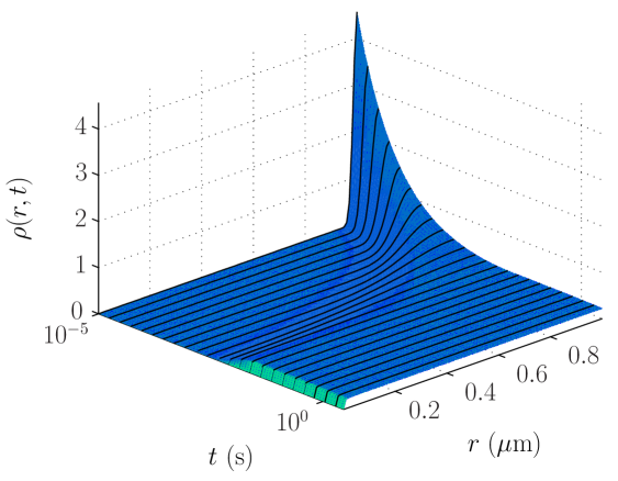
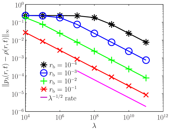
Figure 1: (a) Solution to the Smoluchowski model (7) for rb=103μmsubscript𝑟bsuperscript103𝜇mr_{\textrm{b}}=10^{-3}\mu\textrm{m}. Note that the t𝑡t-axis uses a logarithmic scale. (b) Absolute difference in pλ(r,t)subscript𝑝𝜆𝑟𝑡p_{\lambda}(r,t) and ρ(r,t)𝜌𝑟𝑡\rho(r,t) as λ𝜆\lambda and rbsubscript𝑟br_{\textrm{b}} are varied.

We numerically evaluated pλ(r,t)subscript𝑝𝜆𝑟𝑡p_{\lambda}(r,t) and ρ(r,t)𝜌𝑟𝑡\rho(r,t) in MATLAB using the eigenfunction expansions (10) and (9). The series were truncated at the first term with magnitude smaller than 1010superscript101010^{-10}. In evaluating these series numerically it is necessary to calculate a number of the eigenvalues μnsubscript𝜇𝑛\mu_{n} and αnsubscript𝛼𝑛\alpha_{n}. For each term of the eigenfunction expansions the transcendental equations for the corresponding Doi eigenvalue, f(μn)=A(μn,λ)𝑓subscript𝜇𝑛𝐴subscript𝜇𝑛𝜆f(\mu_{n})=A(\mu_{n},\lambda), and the Smoluchowski eigenvalue, f(αn)=0𝑓subscript𝛼𝑛0f(\alpha_{n})=0, were solved to 25 digits of precision using the Mathematica Reduce function. In Figure 1a we show the solution to the Smoluchowski model (7), ρ(r,t)𝜌𝑟𝑡\rho(r,t), when rb=103μmsubscript𝑟bsuperscript103𝜇mr_{\textrm{b}}=10^{-3}\mu\textrm{m}. For short times the solution is localized near R𝑅R, while a boundary layer develops near r=rb𝑟subscript𝑟br=r_{\textrm{b}} as t𝑡t increases. Figure 1b shows the maximum absolute difference between pλsubscript𝑝𝜆p_{\lambda} and ρ𝜌\rho for a discrete set of points,

pλ(r,t)ρ(r,t)supisupj|pλ(ri,tj)ρ(ri,tj)|,subscriptnormsubscript𝑝𝜆𝑟𝑡𝜌𝑟𝑡subscriptsupremum𝑖subscriptsupremum𝑗subscript𝑝𝜆subscript𝑟𝑖subscript𝑡𝑗𝜌subscript𝑟𝑖subscript𝑡𝑗\|p_{\lambda}(r,t)-\rho(r,t)\|_{\infty}\equiv\sup_{i}\sup_{j}\left|p_{\lambda}(r_{i},t_{j})-\rho(r_{i},t_{j})\right|,

where risubscript𝑟𝑖r_{i} and tjsubscript𝑡𝑗t_{j} are given in Appendix B by Listings 1 and 2. For each fixed value of rbsubscript𝑟br_{\textrm{b}} we see that as λ𝜆\lambda\to\infty the difference between pλsubscript𝑝𝜆p_{\lambda} and ρ𝜌\rho converges to zero like λ1/2superscript𝜆12\lambda^{-1/2}. As rbsubscript𝑟br_{\textrm{b}} is decreased, the absolute difference increases by approximately an order of magnitude for each fixed value of λ𝜆\lambda (for λ𝜆\lambda sufficiently large).

Refer to caption
(a)
Refer to caption
(b)
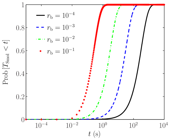
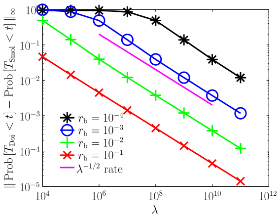
Figure 2: (a) Smoluchowski binding time distributions for varying rbsubscript𝑟br_{\textrm{b}}. Note the t𝑡t-axis is logarithmic. (b) Absolute difference in binding time distributions from the Smoluchowski and Doi models as λ𝜆\lambda is varied.

For many biological models the statistics of the random variable, for the time at which the diffusing molecule first binds to the binding site, are of interest. For example, in [26] we studied how this time was influenced by volume exclusion due to the spatially varying density of chromatin inside the nucleus of mammalian cells. We subsequently denote these random variables by TDoisubscript𝑇DoiT_{\textrm{Doi}} and TSmolsubscript𝑇SmolT_{\textrm{Smol}}. Statistics of these random variables can be calculated from the cumulative distribution functions

Prob[TDoi<t]=14π0Rpλ(r,t)r2𝑑r,Probsubscript𝑇Doi𝑡14𝜋superscriptsubscript0𝑅subscript𝑝𝜆𝑟𝑡superscript𝑟2differential-d𝑟\operatorname{Prob}\left[T_{\textrm{Doi}}<t\right]=1-4\pi\int_{0}^{R}p_{\lambda}(r,t)r^{2}\,dr,

and

Prob[TSmol<t]=14πrbRρ(r,t)r2𝑑r.Probsubscript𝑇Smol𝑡14𝜋superscriptsubscriptsubscript𝑟b𝑅𝜌𝑟𝑡superscript𝑟2differential-d𝑟\operatorname{Prob}\left[T_{\textrm{Smol}}<t\right]=1-4\pi\int_{r_{\textrm{b}}}^{R}\rho(r,t)r^{2}\,dr.

We evaluated Prob[TDoi<t]Probsubscript𝑇Doi𝑡\operatorname{Prob}\left[T_{\textrm{Doi}}<t\right] and Prob[TSmol<t]Probsubscript𝑇Smol𝑡\operatorname{Prob}\left[T_{\textrm{Smol}}<t\right] by analytically integrating the eigenfunction expansions (10) and (9) and evaluating the truncated series in MATLAB. (Using the same method as described above for evaluating pλ(r,t)subscript𝑝𝜆𝑟𝑡p_{\lambda}(r,t) and ρ(r,t)𝜌𝑟𝑡\rho(r,t).)

Figure 2a shows Prob[TSmol<t]Probsubscript𝑇Smol𝑡\operatorname{Prob}\left[T_{\textrm{Smol}}<t\right] for varying rbsubscript𝑟br_{\textrm{b}} and demonstrates a constant increase in the binding time as rbsubscript𝑟br_{\textrm{b}} is decreased (on a logarithmic scale). Figure 2b shows the absolute difference in binding time distributions,

Prob[TDoi<t]Prob[TSmol<t]suptj|Prob[TDoi<tj]Prob[TSmol<tj]|,subscriptnormProbsubscript𝑇Doi𝑡Probsubscript𝑇Smol𝑡subscriptsupremumsubscript𝑡𝑗Probsubscript𝑇Doisubscript𝑡𝑗Probsubscript𝑇Smolsubscript𝑡𝑗\|\operatorname{Prob}\left[T_{\textrm{Doi}}<t\right]-\operatorname{Prob}\left[T_{\textrm{Smol}}<t\right]\|_{\infty}\equiv\sup_{t_{j}}\left|\operatorname{Prob}\left[T_{\textrm{Doi}}<t_{j}\right]-\operatorname{Prob}\left[T_{\textrm{Smol}}<t_{j}\right]\right|,

where tjsubscript𝑡𝑗t_{j} is given by Listing 2 in Appendix B. We again observe an empirical λ12superscript𝜆12\lambda^{-\frac{1}{2}} convergence rate of Prob[TDoi<t]Probsubscript𝑇Doi𝑡\operatorname{Prob}\left[T_{\textrm{Doi}}<t\right] to Prob[TSmol<t]Probsubscript𝑇Smol𝑡\operatorname{Prob}\left[T_{\textrm{Smol}}<t\right] as λ𝜆\lambda\to\infty. For a biologically relevant binding radius of 103μmsuperscript103𝜇m10^{-3}\mu\textrm{m}, when λ=1011s1𝜆superscript1011superscripts1\lambda=10^{11}\textrm{s}^{-1} the absolute difference between the two distributions is on the order of 103superscript10310^{-3}.

Refer to caption
(a)
Refer to caption
(b)
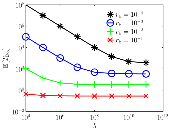
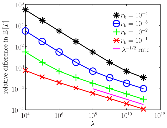
Figure 3: (a) Mean binding time of Doi model vs λ𝜆\lambda. (b) Relative difference in mean binding times (20).

In addition to the probability densities and binding time distributions, we also examined the mean time for the diffusing protein to find the binding site (when starting a distance r0subscript𝑟0r_{0} from the origin). The mean binding time for the Doi model can be found in a simple closed form by solving the corresponding mean first passage time problem (29), see Appendix A, and is given by

𝔼[TDoi](r0)=0Prob[TDoi<t]𝑑t={u(r0),r0<rb,u+(r0),r0>rb.𝔼delimited-[]subscript𝑇Doisubscript𝑟0superscriptsubscript0Probsubscript𝑇Doi𝑡differential-d𝑡casessuperscript𝑢subscript𝑟0subscript𝑟0subscript𝑟botherwisesuperscript𝑢subscript𝑟0subscript𝑟0subscript𝑟botherwise\mathbb{E}\left[T_{\textrm{Doi}}\right](r_{0})=\int_{0}^{\infty}\operatorname{Prob}\left[T_{\textrm{Doi}}<t\right]\,dt=\begin{cases}u^{-}(r_{0}),\quad r_{0}<r_{\textrm{b}},\\ u^{+}(r_{0}),\quad r_{0}>r_{\textrm{b}}.\end{cases} (17)

Where, for λ^=λ/D^𝜆𝜆𝐷\hat{\lambda}=\lambda/D, we have that

u(r0)superscript𝑢subscript𝑟0\displaystyle u^{-}(r_{0}) =1Dλ^+(sinh(λ^r0)r0)[R3rb33D(rbλ^cosh(λ^rb)sinh(λ^rb))],absent1𝐷^𝜆^𝜆subscript𝑟0subscript𝑟0delimited-[]superscript𝑅3superscriptsubscript𝑟b33𝐷subscript𝑟b^𝜆^𝜆subscript𝑟b^𝜆subscript𝑟b\displaystyle=\frac{1}{D\hat{\lambda}}+\left(\frac{\sinh(\sqrt{\hat{\lambda}}r_{0})}{r_{0}}\right)\left[\frac{R^{3}-r_{\textrm{b}}^{3}}{3D\left(r_{\textrm{b}}\sqrt{\hat{\lambda}}\cosh(\sqrt{\hat{\lambda}}r_{\textrm{b}})-\sinh(\sqrt{\hat{\lambda}}r_{\textrm{b}})\right)}\right],
u+(r0)superscript𝑢subscript𝑟0\displaystyle u^{+}(r_{0}) =rb2r026D+R33D[1rb1r0]+1Dλ^+(sinh(λ^rb)rb)[R3rb33D(rbλ^cosh(λ^rb)sinh(λ^rb))].absentsuperscriptsubscript𝑟b2superscriptsubscript𝑟026𝐷superscript𝑅33𝐷delimited-[]1subscript𝑟b1subscript𝑟01𝐷^𝜆^𝜆subscript𝑟bsubscript𝑟bdelimited-[]superscript𝑅3superscriptsubscript𝑟b33𝐷subscript𝑟b^𝜆^𝜆subscript𝑟b^𝜆subscript𝑟b\displaystyle=\frac{r_{\textrm{b}}^{2}-r_{0}^{2}}{6D}+\frac{R^{3}}{3D}\left[\frac{1}{r_{\textrm{b}}}-\frac{1}{r_{0}}\right]+\frac{1}{D\hat{\lambda}}+\left(\frac{\sinh(\sqrt{\hat{\lambda}}r_{\textrm{b}})}{r_{\textrm{b}}}\right)\left[\frac{R^{3}-r_{\textrm{b}}^{3}}{3D\left(r_{\textrm{b}}\sqrt{\hat{\lambda}}\cosh(\sqrt{\hat{\lambda}}r_{\textrm{b}})-\sinh(\sqrt{\hat{\lambda}}r_{\textrm{b}})\right)}\right].

Similarly, the mean binding time in the Smoluchowski model can be found by solving the mean first passage time problem (30), and is given by

𝔼[TSmol](r0)=rb2r026D+R33D[1rb1r0],r0>rb.formulae-sequence𝔼delimited-[]subscript𝑇Smolsubscript𝑟0superscriptsubscript𝑟b2superscriptsubscript𝑟026𝐷superscript𝑅33𝐷delimited-[]1subscript𝑟b1subscript𝑟0subscript𝑟0subscript𝑟b\mathbb{E}\left[T_{\textrm{Smol}}\right](r_{0})=\frac{r_{\textrm{b}}^{2}-r_{0}^{2}}{6D}+\frac{R^{3}}{3D}\left[\frac{1}{r_{\textrm{b}}}-\frac{1}{r_{0}}\right],\quad r_{0}>r_{\textrm{b}}. (18)

Figure 3a shows the mean binding time in the Doi model as λ𝜆\lambda is varied for r0=Rsubscript𝑟0𝑅r_{0}=R.

The difference between the two mean binding times, for r0>rbsubscript𝑟0subscript𝑟br_{0}>r_{\textrm{b}}, is then given by

|𝔼[TDoi](r0)𝔼[TSmol](r0)|𝔼delimited-[]subscript𝑇Doisubscript𝑟0𝔼delimited-[]subscript𝑇Smolsubscript𝑟0\displaystyle\left|\mathbb{E}\left[T_{\textrm{Doi}}\right](r_{0})-\mathbb{E}\left[T_{\textrm{Smol}}\right](r_{0})\right| =|1Dλ^+(sinh(λ^rb)rb)[R3rb33D(rbλ^cosh(λ^rb)sinh(λ^rb))]|.absent1𝐷^𝜆^𝜆subscript𝑟bsubscript𝑟bdelimited-[]superscript𝑅3superscriptsubscript𝑟b33𝐷subscript𝑟b^𝜆^𝜆subscript𝑟b^𝜆subscript𝑟b\displaystyle=\left|\frac{1}{D\hat{\lambda}}+\left(\frac{\sinh(\sqrt{\hat{\lambda}}r_{\textrm{b}})}{r_{\textrm{b}}}\right)\left[\frac{R^{3}-r_{\textrm{b}}^{3}}{3D\left(r_{\textrm{b}}\sqrt{\hat{\lambda}}\cosh(\sqrt{\hat{\lambda}}r_{\textrm{b}})-\sinh(\sqrt{\hat{\lambda}}r_{\textrm{b}})\right)}\right]\right|. (19)

This difference is O(λ12)𝑂superscript𝜆12O(\lambda^{-\frac{1}{2}}), consistent with the results we prove in the next section on the uniform convergence of pλsubscript𝑝𝜆p_{\lambda} to ρ𝜌\rho as λ𝜆\lambda\to\infty. (19) also demonstrates that for large, but fixed values of λ𝜆\lambda the absolute difference in mean binding times will increase like rb1superscriptsubscript𝑟b1r_{\textrm{b}}^{-1} as rbsubscript𝑟br_{\textrm{b}} is decreased. In Figure 3b the relative difference,

|𝔼[TSmol]𝔼[TDoi]|𝔼[TSmol],𝔼delimited-[]subscript𝑇Smol𝔼delimited-[]subscript𝑇Doi𝔼delimited-[]subscript𝑇Smol\frac{\left|\mathbb{E}\left[T_{\textrm{Smol}}\right]-\mathbb{E}\left[T_{\textrm{Doi}}\right]\right|}{\mathbb{E}\left[T_{\textrm{Smol}}\right]}, (20)

is graphed as λ𝜆\lambda is varied for r0=Rsubscript𝑟0𝑅r_{0}=R, illustrating the λ1/2superscript𝜆12\lambda^{-1/2} convergence of 𝔼[TDoi]𝔼delimited-[]subscript𝑇Doi\mathbb{E}\left[T_{\textrm{Doi}}\right] to 𝔼[TSmol]𝔼delimited-[]subscript𝑇Smol\mathbb{E}\left[T_{\textrm{Smol}}\right]. For rb=103μmsubscript𝑟bsuperscript103𝜇mr_{\textrm{b}}=10^{-3}\mu\textrm{m} the mean binding times differ by less than 1%percent11\% when λ=1011s1𝜆superscript1011superscripts1\lambda=10^{11}\,\textrm{s}^{-1}.

Each of Figures 1b2b, and 3b illustrate a λ1/2superscript𝜆12\lambda^{-1/2} empirical convergence rate, consistent with the bound (1) we prove in the next section (Theorem 5.2). Moreover, they demonstrate that as rbsubscript𝑟br_{\textrm{b}} is decreased larger values of λ𝜆\lambda are required to ensure the absolute difference between the two models remains below a fixed tolerance. In all three cases, once λ𝜆\lambda is sufficiently large that the λ1/2superscript𝜆12\lambda^{-1/2} convergence rate can be observed, the absolute difference appears to scale like rb1superscriptsubscript𝑟b1r_{\textrm{b}}^{-1} as rbsubscript𝑟br_{\textrm{b}} is decreased.

5 Rigorous Convergence Results

In this section we study the rigorous relationship between the Doi model (8) and Smoluchowski model (7). In Subsection 5.1 we derive a rigorous error bound on the rate of convergence of the Doi eigenvalues, μn(λ)subscript𝜇𝑛𝜆\mu_{n}(\lambda), to the Smoluchowski eigenvalues, αnsubscript𝛼𝑛\alpha_{n}, as λ𝜆\lambda\to\infty. In Subsection 5.2 we obtain similar estimates for the convergence of the Doi eigenfunctions, ψnoutsubscriptsuperscript𝜓𝑜𝑢𝑡𝑛\psi^{out}_{n}, to the Smoluchowski eigenfunctions, ϕnsubscriptitalic-ϕ𝑛\phi_{n}. We obtain our main result in subsection 5.3 where we use these eigenvalue and eigenfunction estimates to show the uniform convergence in space and time of the solution to the Doi model (8), pλ(r,t)subscript𝑝𝜆𝑟𝑡p_{\lambda}(r,t), to the solution of the Smoluchowski model (7), ρ(r,t)𝜌𝑟𝑡\rho(r,t), as λ𝜆\lambda\to\infty. (With the error bound (1).)

5.1 Eigenvalue Estimates

In this subsection we derive estimates for the difference between the Doi, μn(λ)subscript𝜇𝑛𝜆\mu_{n}(\lambda), and Smoluchowski, αnsubscript𝛼𝑛\alpha_{n}, eigenvalues. We start by proving some properties of the functions A(μ,λ)𝐴𝜇𝜆A(\mu,\lambda) and f(μ)𝑓𝜇f(\mu) that we will find useful:

Proposition 5.1.

A(μ,λ)𝐴𝜇𝜆A(\mu,\lambda) is monotone increasing. Furthermore for μλ𝜇𝜆\mu\leq\lambda, A𝐴A is positive.

Proof.

Positivity is trivial since tanh\tanh is positive. Note also that A(0,λ)=tanh(λrb)/λ𝐴0𝜆𝜆subscript𝑟b𝜆A(0,\lambda)=\tanh(\sqrt{\lambda}r_{\textrm{b}})/\sqrt{\lambda}. A simple computation shows that for μ<λ𝜇𝜆\mu<\lambda

ddμA(μ;λ)=tanh(λμrb)rbλμ(sech2(λμrb))2(λμ)3/2=sinh(2λμrb)2rbλμ4cosh2(λμrb)(λμ)3/2𝑑𝑑𝜇𝐴𝜇𝜆𝜆𝜇subscript𝑟bsubscript𝑟b𝜆𝜇superscriptsech2𝜆𝜇subscript𝑟b2superscript𝜆𝜇322𝜆𝜇subscript𝑟b2subscript𝑟b𝜆𝜇4superscript2𝜆𝜇subscript𝑟bsuperscript𝜆𝜇32\displaystyle\frac{d}{d\mu}A(\mu;\lambda)=\frac{\tanh\left(\sqrt{\lambda-\mu}r_{\textrm{b}}\right)-r_{\textrm{b}}\sqrt{\lambda-\mu}\left(\operatorname{sech}^{2}\left(\sqrt{\lambda-\mu}r_{\textrm{b}}\right)\right)}{2\left(\lambda-\mu\right)^{3/2}}=\frac{\sinh\left(2\sqrt{\lambda-\mu}r_{\textrm{b}}\right)-2r_{\textrm{b}}\sqrt{\lambda-\mu}}{4\cosh^{2}\left(\sqrt{\lambda-\mu}r_{\textrm{b}}\right)\left(\lambda-\mu\right)^{3/2}}

and for μ>λ𝜇𝜆\mu>\lambda

ddμA(μ;λ)=rbμλ(sec2(μλrb))tan(μλrb)2(λμ)3/2=2rbμλsin(2μλrb)4cos2(μλrb)(μλ)3/2.𝑑𝑑𝜇𝐴𝜇𝜆subscript𝑟b𝜇𝜆superscript2𝜇𝜆subscript𝑟b𝜇𝜆subscript𝑟b2superscript𝜆𝜇322subscript𝑟b𝜇𝜆2𝜇𝜆subscript𝑟b4superscript2𝜇𝜆subscript𝑟bsuperscript𝜇𝜆32\displaystyle\frac{d}{d\mu}A(\mu;\lambda)=\frac{r_{\textrm{b}}\sqrt{\mu-\lambda}\left(\sec^{2}\left(\sqrt{\mu-\lambda}r_{\textrm{b}}\right)\right)-\tan\left(\sqrt{\mu-\lambda}r_{\textrm{b}}\right)}{2\left(\lambda-\mu\right)^{3/2}}=\frac{2r_{\textrm{b}}\sqrt{\mu-\lambda}-\sin\left(2\sqrt{\mu-\lambda}r_{\textrm{b}}\right)}{4\cos^{2}\left(\sqrt{\mu-\lambda}r_{\textrm{b}}\right)\left(\mu-\lambda\right)^{3/2}}.

The result follows since for u0𝑢0u\geq 0, sinh(u)u𝑢𝑢\sinh(u)\geq u and sin(u)u𝑢𝑢\sin(u)\leq u. ∎

Let the vertical asymptotes of f(μ)𝑓𝜇f(\mu) be denoted by βnsubscript𝛽𝑛\beta_{n}. They satisfy the equation

Rβntan(βn(Rrb))+βn=0;βn>0.formulae-sequence𝑅subscript𝛽𝑛subscript𝛽𝑛𝑅subscript𝑟bsubscript𝛽𝑛0subscript𝛽𝑛0R\beta_{n}\tan(\sqrt{\beta_{n}}(R-r_{\textrm{b}}))+\sqrt{\beta_{n}}=0;\quad\beta_{n}>0.
Proposition 5.2.

We have the following

  1. 1.

    0<α1<β1<α2<<βn<αn+1<0subscript𝛼1subscript𝛽1subscript𝛼2subscript𝛽𝑛subscript𝛼𝑛10<\alpha_{1}<\beta_{1}<\alpha_{2}<\ldots<\beta_{n}<\alpha_{n+1}<\ldots

  2. 2.

    f(μ)<0superscript𝑓𝜇0f^{\prime}(\mu)<0 and f(μ)>0𝑓𝜇0f(\mu)>0 on [0,α1)0subscript𝛼1[0,\alpha_{1}) and (βn,αn+1)subscript𝛽𝑛subscript𝛼𝑛1(\beta_{n},\alpha_{n+1}) for n1𝑛1n\geq 1.

Proof.

1. Let κ=1rb/R𝜅1subscript𝑟b𝑅\kappa=1-r_{\textrm{b}}/R and x=Rμ𝑥𝑅𝜇x=R\sqrt{\mu}. We make the change of variable in f(μ)𝑓𝜇f(\mu) and obtain

f(μ)f~(x)=R(xtan(κx))x2tan(κx)+x=R(1tan(κx)x)xtan(κx)+1N(x)D(x).𝑓𝜇~𝑓𝑥𝑅𝑥𝜅𝑥superscript𝑥2𝜅𝑥𝑥𝑅1𝜅𝑥𝑥𝑥𝜅𝑥1𝑁𝑥𝐷𝑥f(\mu)\equiv\tilde{f}(x)=\frac{R\left(x-\tan(\kappa x)\right)}{x^{2}\tan(\kappa x)+x}=\frac{R\left(1-\frac{\tan(\kappa x)}{x}\right)}{x\tan(\kappa x)+1}\equiv\frac{N(x)}{D(x)}.

Let dnsubscript𝑑𝑛d_{n} be such that N(dn)=0𝑁subscript𝑑𝑛0N(d_{n})=0 and ηnsubscript𝜂𝑛\eta_{n} be such that D(ηn)=0𝐷subscript𝜂𝑛0D(\eta_{n})=0. In terms of the old variable, we have dn=Rαnsubscript𝑑𝑛𝑅subscript𝛼𝑛d_{n}=R\sqrt{\alpha_{n}} and ηn=Rβnsubscript𝜂𝑛𝑅subscript𝛽𝑛\eta_{n}=R\sqrt{\beta_{n}}. N(x)=0𝑁𝑥0N(x)=0 imply that tan(κx)=x𝜅𝑥𝑥\tan(\kappa x)=x and D(x)=0𝐷𝑥0D(x)=0 imply that tan(κx)=1x𝜅𝑥1𝑥\tan(\kappa x)=-\frac{1}{x}. Note that the functions tan(κx)𝜅𝑥\tan(\kappa x), x𝑥x and 1x1𝑥-\frac{1}{x} are all monotone increasing. Finally if we let θn=π2κ(2n1)subscript𝜃𝑛𝜋2𝜅2𝑛1\theta_{n}=\frac{\pi}{2\kappa}(2n-1) be the vertical asymptotes of tan(κx)𝜅𝑥\tan(\kappa x) one easily checks that we have

0<d1<θ1<η1<<dn<θn<ηn0subscript𝑑1subscript𝜃1subscript𝜂1subscript𝑑𝑛subscript𝜃𝑛subscript𝜂𝑛0<d_{1}<\theta_{1}<\eta_{1}<\ldots<d_{n}<\theta_{n}<\eta_{n}\ldots

This proves 1.

2. N>0𝑁0N>0 on n1(θn,dn+1)(0,d1)subscript𝑛1subscript𝜃𝑛subscript𝑑𝑛10subscript𝑑1\displaystyle\bigcup_{n\geq 1}(\theta_{n},d_{n+1})\cup(0,d_{1}), and N<0𝑁0N<0 on n1(dn,θn)subscript𝑛1subscript𝑑𝑛subscript𝜃𝑛\displaystyle\bigcup_{n\geq 1}(d_{n},\theta_{n}). Similarly, D>0𝐷0D>0 on n1(ηn,θn+1)(0,θ1)subscript𝑛1subscript𝜂𝑛subscript𝜃𝑛10subscript𝜃1\displaystyle\bigcup_{n\geq 1}(\eta_{n},\theta_{n+1})\cup(0,\theta_{1}) and D<0𝐷0D<0 on n1(θn,ηn)subscript𝑛1subscript𝜃𝑛subscript𝜂𝑛\displaystyle\bigcup_{n\geq 1}(\theta_{n},\eta_{n}). Thus it follows that f~(x)>0~𝑓𝑥0\tilde{f}(x)>0 if and only if xn1(ηn,dn+1)(0,d1)𝑥subscript𝑛1subscript𝜂𝑛subscript𝑑𝑛10subscript𝑑1x\in\displaystyle\bigcup_{n\geq 1}(\eta_{n},d_{n+1})\cup(0,d_{1}). Next, we show that f<0superscript𝑓0f^{\prime}<0. Note

N(x)=R(tan(κx)κxsec2(κx))x2=R(sin(2κx)2κx)2x2cos2(κx),superscript𝑁𝑥𝑅𝜅𝑥𝜅𝑥superscript2𝜅𝑥superscript𝑥2𝑅2𝜅𝑥2𝜅𝑥2superscript𝑥2superscript2𝜅𝑥\displaystyle N^{\prime}(x)=\frac{R\left(\tan(\kappa x)-\kappa x\sec^{2}(\kappa x)\right)}{x^{2}}=\frac{R\left(\sin(2\kappa x)-2\kappa x\right)}{2x^{2}\cos^{2}(\kappa x)},

and

D(x)=tan(κx)+κxsec2(κx)=sin(2κx)+2κx2cos2(κx).superscript𝐷𝑥𝜅𝑥𝜅𝑥superscript2𝜅𝑥2𝜅𝑥2𝜅𝑥2superscript2𝜅𝑥\displaystyle D^{\prime}(x)=\tan(\kappa x)+\kappa x\sec^{2}(\kappa x)=\frac{\sin(2\kappa x)+2\kappa x}{2\cos^{2}(\kappa x)}.

Since |sin(θ)||θ|𝜃𝜃\left|\sin(\theta)\right|\leq\left|\theta\right| it follows that N(x)0superscript𝑁𝑥0N^{\prime}(x)\leq 0 and that D(x)0superscript𝐷𝑥0D^{\prime}(x)\geq 0, with equality in both only when x=0𝑥0x=0. From what we have shown above, f~(x)>0~𝑓𝑥0\tilde{f}(x)>0 if and only if both N(x)>0𝑁𝑥0N(x)>0 and D(x)>0𝐷𝑥0D(x)>0 so that

f(μ)=f~(x)dxdμ=[D(x)N(x)N(x)D(x)D(x)2]dxdμ<0.superscript𝑓𝜇superscript~𝑓𝑥𝑑𝑥𝑑𝜇delimited-[]𝐷𝑥superscript𝑁𝑥𝑁𝑥superscript𝐷𝑥𝐷superscript𝑥2𝑑𝑥𝑑𝜇0\displaystyle f^{\prime}(\mu)=\tilde{f}^{\prime}(x)\cdot\frac{dx}{d\mu}=\left[\frac{D(x)N^{\prime}(x)-N(x)D^{\prime}(x)}{{D(x)}^{2}}\right]\cdot\frac{dx}{d\mu}<0.

Proposition 5.3.

The Doi eigenvalues μn(λ)subscript𝜇𝑛𝜆\mu_{n}(\lambda) satisfy for n𝑛n such that μn(λ)λsubscript𝜇𝑛𝜆𝜆\mu_{n}(\lambda)\leq\lambda

0<μ1(λ)<α1<β1<μ2(λ)<α2<<βn1<μn(λ)<αn0subscript𝜇1𝜆subscript𝛼1subscript𝛽1subscript𝜇2𝜆subscript𝛼2subscript𝛽𝑛1subscript𝜇𝑛𝜆subscript𝛼𝑛0<\mu_{1}(\lambda)<\alpha_{1}<\beta_{1}<\mu_{2}(\lambda)<\alpha_{2}<\ldots<\beta_{n-1}<\mu_{n}(\lambda)<\alpha_{n}
Proof.

This follows from the fact that f(μ)𝑓𝜇f(\mu) is decreasing wherever it is positive and that A(μ;λ)𝐴𝜇𝜆A(\mu;\lambda) is positive and increasing for μλ𝜇𝜆\mu\leq\lambda. ∎

We will also have need for the following

Proposition 5.4.

Let {γn}subscript𝛾𝑛\{\gamma_{n}\} denote the eigenvalues for the (positive) radially symmetric Laplacian on [0,R)0𝑅\left[0,R\right), with zero Neumann boundary conditions on the ball of radius R𝑅R. Let αnsubscript𝛼𝑛\alpha_{n} and μnsubscript𝜇𝑛\mu_{n} be as above. Then the following hold:

  1. 1.

    The μn(λ)subscript𝜇𝑛𝜆\mu_{n}(\lambda) are continuous and monotone increasing in λ𝜆\lambda for all n1𝑛1n\geq 1

  2. 2.

    For all n1𝑛1n\geq 1 and any fixed λ𝜆\lambda, we have that

    μn(0)=γn=((n1)πR)2μn(λ)subscript𝜇𝑛0subscript𝛾𝑛superscript𝑛1𝜋𝑅2subscript𝜇𝑛𝜆\mu_{n}(0)=\gamma_{n}=\left(\frac{(n-1)\pi}{R}\right)^{2}\leq\mu_{n}(\lambda)
Remark 5.1.

The proof is a straightforward application of the variational minimax principle of Poincare. We do not show it here.

Proposition 5.5.

For any L+𝐿subscriptL\in\mathbb{R}_{+}, define the index set 𝒜(L)={n|αnL}𝒜𝐿conditional-set𝑛subscript𝛼𝑛𝐿\mathcal{A}(L)=\{n|\alpha_{n}\leq L\}. If we let |𝒜(L)|card(𝒜(L))𝒜𝐿card𝒜𝐿\left|\mathcal{A}(L)\right|\equiv\operatorname{card}(\mathcal{A}(L)) then given δ>0𝛿0\delta>0 there exists constants C1(δ)superscriptsubscript𝐶1𝛿C_{1}^{*}(\delta) and C2(δ)superscriptsubscript𝐶2𝛿C_{2}^{*}(\delta) such that for Lδ𝐿𝛿L\geq\delta

C1(δ)L|𝒜(L)|C2(δ)Lsuperscriptsubscript𝐶1𝛿𝐿𝒜𝐿superscriptsubscript𝐶2𝛿𝐿C_{1}^{*}(\delta)\sqrt{L}\leq\left|\mathcal{A}(L)\right|\leq C_{2}^{*}(\delta)\sqrt{L} (21)
Proof.

Write L~=RL~𝐿𝑅𝐿\widetilde{L}=R\sqrt{L} and again define κ=1rb/R𝜅1subscript𝑟b𝑅\kappa=1-r_{\textrm{b}}/R. Then |𝒜(L)|𝒜𝐿\left|\mathcal{A}(L)\right| is just the number of solutions to tan(κx)=x𝜅𝑥𝑥\tan(\kappa x)=x which lie in the interval [0,L~]0~𝐿[0,\widetilde{L}]. This number is well approximated by the number of vertical asymptotes of tan(κx)𝜅𝑥\tan(\kappa x). It then follows that

κL~π1|𝒜(L)|κL~π+1𝜅~𝐿𝜋1𝒜𝐿𝜅~𝐿𝜋1\frac{\kappa\widetilde{L}}{\pi}-1\leq\left|\mathcal{A}(L)\right|\leq\frac{\kappa\widetilde{L}}{\pi}+1

so that

L(Rrbπ1L)|𝒜(L)|L(Rrbπ+1L).𝐿𝑅subscript𝑟b𝜋1𝐿𝒜𝐿𝐿𝑅subscript𝑟b𝜋1𝐿\sqrt{L}\left(\frac{R-r_{\textrm{b}}}{\pi}-\frac{1}{\sqrt{L}}\right)\leq\left|\mathcal{A}(L)\right|\leq\sqrt{L}\left(\frac{R-r_{\textrm{b}}}{\pi}+\frac{1}{\sqrt{L}}\right).

If Lδ𝐿𝛿L\geq\delta the choice C1(δ)=Rrbπ1δsuperscriptsubscript𝐶1𝛿𝑅subscript𝑟b𝜋1𝛿\displaystyle C_{1}^{*}(\delta)=\frac{R-r_{\textrm{b}}}{\pi}-\frac{1}{\sqrt{\delta}} and C2(δ)=Rrbπ+1δsuperscriptsubscript𝐶2𝛿𝑅subscript𝑟b𝜋1𝛿\displaystyle C_{2}^{*}(\delta)=\frac{R-r_{\textrm{b}}}{\pi}+\frac{1}{\sqrt{\delta}} gives the proposition.

Remark 5.2.

In practice we will choose δ=4π2/(Rrb)2𝛿4superscript𝜋2superscript𝑅subscript𝑟b2\delta=4\pi^{2}/(R-r_{\textrm{b}})^{2} so that C1=(Rrb)/2πsuperscriptsubscript𝐶1𝑅subscript𝑟b2𝜋C_{1}^{*}=(R-r_{\textrm{b}})/2\pi.

We now give our main convergence estimate for the eigenvalues of the Doi model. The following theorem can be regarded as the heart of the subsequent computations.

Theorem 5.1.

Let 0<σ0<140subscript𝜎0140<\sigma_{0}<\tfrac{1}{4} and define M(λ)K0λσ𝑀𝜆subscript𝐾0superscript𝜆𝜎M(\lambda)\equiv K_{0}\lambda^{\sigma} for K0>1subscript𝐾01K_{0}>1. For any fixed σ(0,σ0]𝜎0subscript𝜎0\sigma\in(0,\sigma_{0}] there exists λ0>0subscript𝜆00\lambda_{0}>0 such that for λλ0𝜆subscript𝜆0\lambda\geq\lambda_{0}, M(λ)λ12𝑀𝜆𝜆12\frac{M(\lambda)}{\lambda}\leq\frac{1}{2}. Then for αnM(λ)subscript𝛼𝑛𝑀𝜆\alpha_{n}\leq M(\lambda), μn(λ)αnsubscript𝜇𝑛𝜆subscript𝛼𝑛\mu_{n}(\lambda)\to\alpha_{n}, 𝒪(λ(122σ))𝒪superscript𝜆122𝜎\mathcal{O}(\lambda^{-(\frac{1}{2}-2\sigma)}).

Remark 5.3.

Note that in the remainder C𝐶C will denote an arbitrary constant that may depend on R𝑅R, rbsubscript𝑟br_{\textrm{b}}, and λ0subscript𝜆0\lambda_{0}. We will also subsequently assume λ0>1subscript𝜆01\lambda_{0}>1.

Proof.

Recall that the Doi eigenvalues μn(λ)subscript𝜇𝑛𝜆\mu_{n}(\lambda) satisfy

f(μn(λ))=A(μn(λ),λ).𝑓subscript𝜇𝑛𝜆𝐴subscript𝜇𝑛𝜆𝜆f(\mu_{n}(\lambda))=A(\mu_{n}(\lambda),\lambda).

As before let κ=1rb/R𝜅1subscript𝑟b𝑅\kappa=1-r_{\textrm{b}}/R and let x=Rμ𝑥𝑅𝜇x=R\sqrt{\mu}. Recalling the definitions of D(x)𝐷𝑥D(x) and N(x)𝑁𝑥N(x) from Proposition 5.2, define

B(x;λ)=D(x)A~(x,λ)[xtan(κx)+1]tanh(rb1x2λR2)λ1x2λR2.𝐵𝑥𝜆𝐷𝑥~𝐴𝑥𝜆delimited-[]𝑥𝜅𝑥1subscript𝑟b1superscript𝑥2𝜆superscript𝑅2𝜆1superscript𝑥2𝜆superscript𝑅2B(x;\lambda)=D(x)\tilde{A}(x,\lambda)\equiv\frac{\left[x\tan(\kappa x)+1\right]\tanh\left(r_{\textrm{b}}\sqrt{1-\frac{x^{2}}{\lambda R^{2}}}\right)}{\sqrt{\lambda}\sqrt{1-\frac{x^{2}}{\lambda R^{2}}}}.

It follows that the rescaled Doi eigenvalues xn(λ)subscript𝑥𝑛𝜆x_{n}(\lambda) satisfy

N(xn(λ))=B(xn(λ);λ).𝑁subscript𝑥𝑛𝜆𝐵subscript𝑥𝑛𝜆𝜆N(x_{n}(\lambda))=B(x_{n}(\lambda);\lambda).

For K0>1subscript𝐾01K_{0}>1 we choose λ(2K0)11σ0𝜆superscript2subscript𝐾011subscript𝜎0\lambda\geq(2K_{0})^{\frac{1}{1-\sigma_{0}}} so that M(λ)λ12𝑀𝜆𝜆12\frac{M(\lambda)}{\lambda}\leq\frac{1}{2}. Recall f(μ)f~(x)𝑓𝜇~𝑓𝑥f(\mu)\equiv\tilde{f}(x). We restrict to {x:x2R2M(λ),f~(x)0}conditional-set𝑥formulae-sequencesuperscript𝑥2superscript𝑅2𝑀𝜆~𝑓𝑥0\{x:\frac{x^{2}}{R^{2}}\leq M(\lambda),\tilde{f}(x)\geq 0\}, and let h(u)=(1u)1/2𝑢superscript1𝑢12h(u)=(1-u)^{-1/2}. Since hh is monotone it follows that

1λ1x2λR2h(x2R2λ)λh(12)λ=2λ.1𝜆1superscript𝑥2𝜆superscript𝑅2superscript𝑥2superscript𝑅2𝜆𝜆12𝜆2𝜆\frac{1}{\sqrt{\lambda}\sqrt{1-\frac{x^{2}}{\lambda R^{2}}}}\equiv\frac{h(\tfrac{x^{2}}{R^{2}\lambda})}{\sqrt{\lambda}}\leq\frac{h(\tfrac{1}{2})}{\sqrt{\lambda}}=\frac{\sqrt{2}}{\sqrt{\lambda}}.

As shown in Proposition 5.2, f~(x)0~𝑓𝑥0\tilde{f}(x)\geq 0 implies 1xtan(κx)x1𝑥𝜅𝑥𝑥-\frac{1}{x}\leq\tan(\kappa x)\leq x so that

|B(x;λ)|[1+xtan(κx)]2λ[1+x2]2λ.𝐵𝑥𝜆delimited-[]1𝑥𝜅𝑥2𝜆delimited-[]1superscript𝑥22𝜆\displaystyle\left|B(x;\lambda)\right|\leq\frac{\left[1+x\tan(\kappa x)\right]\sqrt{2}}{\sqrt{\lambda}}\leq\frac{\left[1+x^{2}\right]\sqrt{2}}{\sqrt{\lambda}}.

Write xn(λ)=dnϵnsubscript𝑥𝑛𝜆subscript𝑑𝑛subscriptitalic-ϵ𝑛x_{n}(\lambda)=d_{n}-\epsilon_{n}. (Recall dn=Rαnsubscript𝑑𝑛𝑅subscript𝛼𝑛d_{n}=R\sqrt{\alpha_{n}} and ηn=Rβnsubscript𝜂𝑛𝑅subscript𝛽𝑛\eta_{n}=R\sqrt{\beta_{n}}.) Then

N(dnϵn)=B(xn(λ);λ).𝑁subscript𝑑𝑛subscriptitalic-ϵ𝑛𝐵subscript𝑥𝑛𝜆𝜆N(d_{n}-\epsilon_{n})=B(x_{n}(\lambda);\lambda).

Applying the mean value theorem we get, for some en(xn(λ),dn)subscript𝑒𝑛subscript𝑥𝑛𝜆subscript𝑑𝑛e_{n}\in(x_{n}(\lambda),d_{n}), that

N(dn)N(en)ϵn=B(xn(λ);λ).𝑁subscript𝑑𝑛superscript𝑁subscript𝑒𝑛subscriptitalic-ϵ𝑛𝐵subscript𝑥𝑛𝜆𝜆N(d_{n})-N^{\prime}(e_{n})\epsilon_{n}=B(x_{n}(\lambda);\lambda).

As N(dn)=0𝑁subscript𝑑𝑛0N(d_{n})=0 and N(en)<0superscript𝑁subscript𝑒𝑛0N^{\prime}(e_{n})<0,

|N(en)|ϵn[1+xn2]2λsuperscript𝑁subscript𝑒𝑛subscriptitalic-ϵ𝑛delimited-[]1superscriptsubscript𝑥𝑛22𝜆\left|N^{\prime}(e_{n})\right|\epsilon_{n}\leq\frac{\left[1+x_{n}^{2}\right]\sqrt{2}}{\sqrt{\lambda}}

which gives that

ϵnsubscriptitalic-ϵ𝑛\displaystyle\epsilon_{n} 2[1+xn2](2en2cos2(κen))Rλ(2κensin(2κen))2[1+dn2]enκRλ(1sin(2κen)2κen)C[1+dn2]dnλ(1sin(2κen)2κen)absent2delimited-[]1subscriptsuperscript𝑥2𝑛2superscriptsubscript𝑒𝑛2superscript2𝜅subscript𝑒𝑛𝑅𝜆2𝜅subscript𝑒𝑛2𝜅subscript𝑒𝑛2delimited-[]1subscriptsuperscript𝑑2𝑛subscript𝑒𝑛𝜅𝑅𝜆12𝜅subscript𝑒𝑛2𝜅subscript𝑒𝑛𝐶delimited-[]1subscriptsuperscript𝑑2𝑛subscript𝑑𝑛𝜆12𝜅subscript𝑒𝑛2𝜅subscript𝑒𝑛\displaystyle\leq\frac{\sqrt{2}\left[1+x^{2}_{n}\right]\left(2e_{n}^{2}\cos^{2}(\kappa e_{n})\right)}{R\sqrt{\lambda}\left(2\kappa e_{n}-\sin(2\kappa e_{n})\right)}\leq\frac{\sqrt{2}\left[1+d^{2}_{n}\right]e_{n}}{\kappa R\sqrt{\lambda}\left(1-\tfrac{\sin(2\kappa e_{n})}{2\kappa e_{n}}\right)}\leq\frac{C\left[1+d^{2}_{n}\right]d_{n}}{\sqrt{\lambda}\left(1-\tfrac{\sin(2\kappa e_{n})}{2\kappa e_{n}}\right)} (22)

For any fixed c(0,κx1(1))𝑐0𝜅subscript𝑥11c\in\left(0,\kappa\,x_{1}(1)\right), monotonicity of the eigenvalues implies 0<c2κx1(λ0)xn(λ)<en<dn0𝑐2𝜅subscript𝑥1subscript𝜆0subscript𝑥𝑛𝜆subscript𝑒𝑛subscript𝑑𝑛0<\frac{c}{2\kappa}\leq x_{1}(\lambda_{0})\leq x_{n}(\lambda)<e_{n}<d_{n}, and therefore c<2κen𝑐2𝜅subscript𝑒𝑛c<2\kappa e_{n}. Define l(θ)=1sin(θ)θ𝑙𝜃1𝜃𝜃\displaystyle l(\theta)=1-\frac{\sin(\theta)}{\theta}. It follows easily that for θc𝜃𝑐\theta\geq c there exists 0<m<10𝑚10<m<1 such that

ml(θ)1𝑚𝑙𝜃1m\leq l(\theta)\leq 1

Using this bound in (22), in the original unscaled variables we find that

R(αnμn)𝑅subscript𝛼𝑛subscript𝜇𝑛\displaystyle R(\sqrt{\alpha_{n}}-\sqrt{\mu_{n}}) CRαn[1+R2αn]λabsent𝐶𝑅subscript𝛼𝑛delimited-[]1superscript𝑅2subscript𝛼𝑛𝜆\displaystyle\leq\frac{CR\sqrt{\alpha_{n}}\left[1+R^{2}\alpha_{n}\right]}{\sqrt{\lambda}} (23)

which implies

αnμnsubscript𝛼𝑛subscript𝜇𝑛\displaystyle\alpha_{n}-\mu_{n} 2Cαn[1+R2αn]λ.absent2𝐶subscript𝛼𝑛delimited-[]1superscript𝑅2subscript𝛼𝑛𝜆\displaystyle\leq\frac{2C\alpha_{n}\left[1+R^{2}\alpha_{n}\right]}{\sqrt{\lambda}}.

For αnM(λ)K0λσsubscript𝛼𝑛𝑀𝜆subscript𝐾0superscript𝜆𝜎\alpha_{n}\leq M(\lambda)\equiv K_{0}\lambda^{\sigma}, M(λ)>1𝑀𝜆1M(\lambda)>1 implies

αnμnsubscript𝛼𝑛subscript𝜇𝑛\displaystyle\alpha_{n}-\mu_{n} C(M(λ))2λCK02λ122σ.absent𝐶superscript𝑀𝜆2𝜆𝐶superscriptsubscript𝐾02superscript𝜆122𝜎\displaystyle\leq\frac{C(M(\lambda))^{2}}{\sqrt{\lambda}}\equiv\frac{CK_{0}^{2}}{\lambda^{\frac{1}{2}-2\sigma}}.

Remark 5.4.

Of interest is the possibility of tighter estimates here. In fact, one can show that if f′′(μ)>0superscript𝑓′′𝜇0f^{\prime\prime}(\mu)>0 wherever f(μ)>0𝑓𝜇0f(\mu)>0 we actually have

αnμnCαnλ12.subscript𝛼𝑛subscript𝜇𝑛𝐶subscript𝛼𝑛superscript𝜆12\alpha_{n}-\mu_{n}\leq\frac{C\alpha_{n}}{\lambda^{\frac{1}{2}}}.

Theorem 5.1 and Proposition 5.4 immediately implies

Corollary 5.1.

For any fixed n𝑛n, we have that μn(λ)subscript𝜇𝑛𝜆\mu_{n}(\lambda) converges monotonically to αnsubscript𝛼𝑛\alpha_{n} as λ𝜆\lambda\to\infty.

5.2 Eigenfunction Estimates

In this subsection we carry over the estimates for the eigenvalues obtained in the last subsection to obtain the uniform convergence in r𝑟r of the eigenfunctions as λ𝜆\lambda\to\infty. Though unstated, in the remainder all theorems and lemmas include the assumptions of Theorem 5.1.

Lemma 5.1.

The (unnormalized) Doi and Smoluchowski eigenfunctions satisfy

supr[rb,R]|ϕn(r)ψnout(r)|=𝒪(λ(123σ2))subscriptsupremum𝑟subscript𝑟b𝑅subscriptitalic-ϕ𝑛𝑟subscriptsuperscript𝜓𝑜𝑢𝑡𝑛𝑟𝒪superscript𝜆123𝜎2\sup_{r\in[r_{\textrm{b}},R]}{\left|\phi_{n}(r)-\psi^{out}_{n}(r)\right|}=\mathcal{O}\left(\lambda^{-(\frac{1}{2}-\frac{3\sigma}{2})}\right)

for μn<M(λ)=K0λσsubscript𝜇𝑛𝑀𝜆subscript𝐾0superscript𝜆𝜎\mu_{n}<M(\lambda)=K_{0}\lambda^{\sigma} as λ𝜆\lambda\to\infty.

Proof.
|ϕn(r)ψnout(r)|subscriptitalic-ϕ𝑛𝑟subscriptsuperscript𝜓𝑜𝑢𝑡𝑛𝑟\displaystyle\left|\phi_{n}(r)-\psi^{out}_{n}(r)\right| 1r|sin(αn(Rr))Rαnsin(μn(Rr))Rμn|+1r|cos(μn(Rr))cos(αn(Rr))|absent1𝑟subscript𝛼𝑛𝑅𝑟𝑅subscript𝛼𝑛subscript𝜇𝑛𝑅𝑟𝑅subscript𝜇𝑛1𝑟subscript𝜇𝑛𝑅𝑟subscript𝛼𝑛𝑅𝑟\displaystyle\leq\frac{1}{r}\left|{\frac{\sin(\sqrt{\alpha_{n}}(R-r))}{R\sqrt{\alpha_{n}}}-\frac{\sin(\sqrt{\mu_{n}}(R-r))}{R\sqrt{\mu_{n}}}}\right|+\frac{1}{r}\bigg{|}\cos(\sqrt{\mu_{n}}(R-r))-\cos(\sqrt{\alpha_{n}}(R-r))\bigg{|}
:=I+IIassignabsent𝐼𝐼𝐼\displaystyle:=I+II

Note that

I𝐼\displaystyle I 1rb|sin(αn(Rr))Rαnsin(μn(Rr))Rαn|+1rb|sin(μn(Rr))Rαnsin(μn(Rr))Rμn|absent1subscript𝑟bsubscript𝛼𝑛𝑅𝑟𝑅subscript𝛼𝑛subscript𝜇𝑛𝑅𝑟𝑅subscript𝛼𝑛1subscript𝑟bsubscript𝜇𝑛𝑅𝑟𝑅subscript𝛼𝑛subscript𝜇𝑛𝑅𝑟𝑅subscript𝜇𝑛\displaystyle\leq\frac{1}{r_{\textrm{b}}}\left|\frac{\sin(\sqrt{\alpha_{n}}(R-r))}{R\sqrt{\alpha_{n}}}-\frac{\sin(\sqrt{\mu_{n}}(R-r))}{R\sqrt{\alpha_{n}}}\right|+\frac{1}{r_{\textrm{b}}}\left|\frac{\sin(\sqrt{\mu_{n}}(R-r))}{R\sqrt{\alpha_{n}}}-\frac{\sin(\sqrt{\mu_{n}}(R-r))}{R\sqrt{\mu_{n}}}\right|
:=Ia+Ib.assignabsentsubscript𝐼𝑎subscript𝐼𝑏\displaystyle:=I_{a}+I_{b}.

We find

Iasubscript𝐼𝑎\displaystyle I_{a} 1Rrbαn|2sin((Rr)αnμn2)cos((Rr)αn+μn2)|(Rrb)(αnμn)Rrbαn.absent1𝑅subscript𝑟bsubscript𝛼𝑛2𝑅𝑟subscript𝛼𝑛subscript𝜇𝑛2𝑅𝑟subscript𝛼𝑛subscript𝜇𝑛2𝑅subscript𝑟bsubscript𝛼𝑛subscript𝜇𝑛𝑅subscript𝑟bsubscript𝛼𝑛\displaystyle\leq\frac{1}{Rr_{\textrm{b}}\sqrt{\alpha_{n}}}\left|2\sin\left((R-r)\frac{\sqrt{\alpha_{n}}-\sqrt{\mu_{n}}}{2}\right)\cos\left((R-r)\frac{\sqrt{\alpha_{n}}+\sqrt{\mu_{n}}}{2}\right)\right|\leq\frac{(R-r_{\textrm{b}})\left(\sqrt{\alpha_{n}}-\sqrt{\mu_{n}}\right)}{Rr_{\textrm{b}}\sqrt{\alpha_{n}}}.

Similarly we have

Ibsubscript𝐼𝑏\displaystyle I_{b} |sin(μn(Rr))|Rrb[1μn1αn](Rrb)Rrb[αnμnαn].absentsubscript𝜇𝑛𝑅𝑟𝑅subscript𝑟bdelimited-[]1subscript𝜇𝑛1subscript𝛼𝑛𝑅subscript𝑟b𝑅subscript𝑟bdelimited-[]subscript𝛼𝑛subscript𝜇𝑛subscript𝛼𝑛\displaystyle\leq\frac{\left|\sin(\sqrt{\mu_{n}}(R-r))\right|}{Rr_{\textrm{b}}}\left[\frac{1}{\sqrt{\mu_{n}}}-\frac{1}{\sqrt{\alpha_{n}}}\right]\leq\frac{(R-r_{\textrm{b}})}{Rr_{\textrm{b}}}\left[\frac{\sqrt{\alpha_{n}}-\sqrt{\mu_{n}}}{\sqrt{\alpha_{n}}}\right].

Combining these with (23)

I𝐼\displaystyle I C[1+R2αn]λCM(λ)λ=CK0λ12σ.absent𝐶delimited-[]1superscript𝑅2subscript𝛼𝑛𝜆𝐶𝑀𝜆𝜆𝐶subscript𝐾0superscript𝜆12𝜎\displaystyle\leq\frac{C\left[1+R^{2}\alpha_{n}\right]}{\sqrt{\lambda}}\leq\frac{CM(\lambda)}{\sqrt{\lambda}}=\frac{CK_{0}}{\lambda^{\frac{1}{2}-\sigma}}.

For II𝐼𝐼II we have

II𝐼𝐼\displaystyle II 1rb[2sin((Rr)αnμn2)sin((Rr)αn+μn2)]absent1subscript𝑟bdelimited-[]2𝑅𝑟subscript𝛼𝑛subscript𝜇𝑛2𝑅𝑟subscript𝛼𝑛subscript𝜇𝑛2\displaystyle\leq\frac{1}{r_{\textrm{b}}}\left[2\sin\left((R-r)\frac{\sqrt{\alpha_{n}}-\sqrt{\mu_{n}}}{2}\right)\sin\left((R-r)\frac{\sqrt{\alpha_{n}}+\sqrt{\mu_{n}}}{2}\right)\right]
Rrbrb(αnμn)absent𝑅subscript𝑟bsubscript𝑟bsubscript𝛼𝑛subscript𝜇𝑛\displaystyle\leq\frac{R-r_{\textrm{b}}}{r_{\textrm{b}}}(\sqrt{\alpha_{n}}-\sqrt{\mu_{n}})
C(Rrb)αn[1+R2αn]rbλabsent𝐶𝑅subscript𝑟bsubscript𝛼𝑛delimited-[]1superscript𝑅2subscript𝛼𝑛subscript𝑟b𝜆\displaystyle\leq\frac{C(R-r_{\textrm{b}})\sqrt{\alpha_{n}}\left[1+R^{2}\alpha_{n}\right]}{r_{\textrm{b}}\sqrt{\lambda}}
C(M(λ))32λ=CK032λ123σ2.absent𝐶superscript𝑀𝜆32𝜆𝐶superscriptsubscript𝐾032superscript𝜆123𝜎2\displaystyle\leq\frac{C\left(M(\lambda)\right)^{\frac{3}{2}}}{\sqrt{\lambda}}=\frac{CK_{0}^{\frac{3}{2}}}{\lambda^{\frac{1}{2}-\frac{3\sigma}{2}}}.

It follows that

|ϕn(r)ψnout(r)|CK0λ123σ2[1λσ/2+K0]C1(rb,R,K0)λ123σ2subscriptitalic-ϕ𝑛𝑟subscriptsuperscript𝜓𝑜𝑢𝑡𝑛𝑟𝐶subscript𝐾0superscript𝜆123𝜎2delimited-[]1superscript𝜆𝜎2subscript𝐾0subscript𝐶1subscript𝑟b𝑅subscript𝐾0superscript𝜆123𝜎2\left|\phi_{n}(r)-\psi^{out}_{n}(r)\right|\leq\frac{CK_{0}}{\lambda^{\frac{1}{2}-\frac{3\sigma}{2}}}\left[\frac{1}{\lambda^{\sigma/2}}+\sqrt{K_{0}}\right]\leq\frac{C_{1}(r_{\textrm{b}},R,K_{0})}{\lambda^{\frac{1}{2}-\frac{3\sigma}{2}}} (24)

This concludes the proof. ∎

We now prove several uniform properties of the eigenfunctions we will use in the next subsection.

Lemma 5.2.
  1. 1.

    There exist a λ0subscript𝜆0\lambda_{0}, C2=C2(rb,R)subscript𝐶2subscript𝐶2subscript𝑟b𝑅C_{2}=C_{2}(r_{\textrm{b}},R), such that for all λλ0𝜆subscript𝜆0\lambda\geq\lambda_{0} and n+𝑛superscriptn\in\mathbb{Z}^{+}

    max(supr[rb,R]|ψnout(r)|,supr[rb,R]|ϕn(r)|)C2.subscriptsupremum𝑟subscript𝑟b𝑅superscriptsubscript𝜓𝑛𝑜𝑢𝑡𝑟subscriptsupremum𝑟subscript𝑟b𝑅subscriptitalic-ϕ𝑛𝑟subscript𝐶2\max\left(\sup_{r\in[r_{\textrm{b}},R]}\left|\psi_{n}^{out}(r)\right|,\sup_{r\in[r_{\textrm{b}},R]}\left|\phi_{n}(r)\right|\right)\leq C_{2}. (25)
  2. 2.

    Let bn=ψn22subscript𝑏𝑛subscriptsuperscriptnormsubscript𝜓𝑛22b_{n}=\|\psi_{n}\|^{-2}_{2} and an=ϕn22subscript𝑎𝑛subscriptsuperscriptnormsubscriptitalic-ϕ𝑛22a_{n}=\|\phi_{n}\|^{-2}_{2}. Then there exists C3subscript𝐶3C_{3} such that for all λλ0𝜆subscript𝜆0\lambda\geq\lambda_{0}

    max(supn{an},supn{bn})C3.subscriptsupremum𝑛subscript𝑎𝑛subscriptsupremum𝑛subscript𝑏𝑛subscript𝐶3\displaystyle\max\Big{(}\sup_{n}\{a_{n}\},\,\sup_{n}\{b_{n}\}\Big{)}\leq C_{3}. (26)
Proof.

1. We start by defining for z0𝑧0z\geq 0, and rbrRsubscript𝑟b𝑟𝑅r_{\textrm{b}}\leq r\leq R the auxiliary function

H(z,r):=1r[sin(z(Rr))Rzcos(z(Rr))].assign𝐻𝑧𝑟1𝑟delimited-[]𝑧𝑅𝑟𝑅𝑧𝑧𝑅𝑟H(z,r):=\frac{1}{r}\left[\frac{\sin(\sqrt{z}(R-r))}{R\sqrt{z}}-\cos(\sqrt{z}(R-r))\right].

Note ϕn(r)H(αn,r)subscriptitalic-ϕ𝑛𝑟𝐻subscript𝛼𝑛𝑟\phi_{n}(r)\equiv H(\alpha_{n},r) and ψnout(r)H(μn,r)superscriptsubscript𝜓𝑛𝑜𝑢𝑡𝑟𝐻subscript𝜇𝑛𝑟\psi_{n}^{out}(r)\equiv H(\mu_{n},r). Now for zz0>0𝑧subscript𝑧00z\geq z_{0}>0 we have that

|H(z,r)|𝐻𝑧𝑟\displaystyle\left|H(z,r)\right| =1r|[sin(z(Rr))Rzcos(z(Rr))]|absent1𝑟delimited-[]𝑧𝑅𝑟𝑅𝑧𝑧𝑅𝑟\displaystyle=\frac{1}{r}\left|\left[\frac{\sin(\sqrt{z}(R-r))}{R\sqrt{z}}-\cos(\sqrt{z}(R-r))\right]\right|
1rb[1Rz+1]absent1subscript𝑟bdelimited-[]1𝑅𝑧1\displaystyle\leq\frac{1}{r_{\textrm{b}}}\left[\frac{1}{R\sqrt{z}}+1\right]
1rb[1Rz0+1]=:C2(z0).\displaystyle\leq\frac{1}{r_{\textrm{b}}}\left[\frac{1}{R\sqrt{z_{0}}}+1\right]=:C_{2}(z_{0}).

By Corollary 5.1 there exists λ0subscript𝜆0\lambda_{0} such that for λλ0𝜆subscript𝜆0\lambda\geq\lambda_{0}

α1μ1(λ)μ1(λ0)α12>0.subscript𝛼1subscript𝜇1𝜆subscript𝜇1subscript𝜆0subscript𝛼120\alpha_{1}\geq\mu_{1}(\lambda)\geq\mu_{1}(\lambda_{0})\geq\frac{\alpha_{1}}{2}>0.

Note that we are using the fact that both the Doi and Smoluchowski eigenvalues can be written in non-decreasing order. Choosing z0=α1/2subscript𝑧0subscript𝛼12z_{0}=\alpha_{1}/2, proves the first part of the lemma.

2. To prove the second part start by defining

h(z):=rbR(H(z,r))2r2𝑑r.assign𝑧superscriptsubscriptsubscript𝑟b𝑅superscript𝐻𝑧𝑟2superscript𝑟2differential-d𝑟h(z):=\int_{r_{\textrm{b}}}^{R}{\left(H(z,r)\right)^{2}r^{2}\,dr}.

Once again we have that ψnout22h(μn)subscriptsuperscriptnormsubscriptsuperscript𝜓𝑜𝑢𝑡𝑛22subscript𝜇𝑛\|\psi^{out}_{n}\|^{2}_{2}\equiv h(\mu_{n}) and ϕn22h(αn)subscriptsuperscriptnormsubscriptitalic-ϕ𝑛22subscript𝛼𝑛\|\phi_{n}\|^{2}_{2}\equiv h(\alpha_{n}). A priori we have that h(z)>0𝑧0h(z)>0 for all z0𝑧0z\geq 0. An explicit computation shows that for z>0𝑧0z>0, h(z)𝑧h(z) is continuous, limzh(z)=(Rrb)/2>0subscript𝑧𝑧𝑅subscript𝑟b20\lim\limits_{z\to\infty}h(z)=(R-r_{\textrm{b}})/2>0, and limz0h(z)=(R3rb3)/3R2subscript𝑧0𝑧superscript𝑅3superscriptsubscript𝑟b33superscript𝑅2\lim\limits_{z\to 0}h(z)=(R^{3}-r_{\textrm{b}}^{3})/3R^{2}. With the positivity of h(z)𝑧h(z) on [0,)0\left[0,\infty\right), these results imply that A:=infh(z)>0assign𝐴infimum𝑧0A:=\inf h(z)>0. It then follows that

an=1ϕn221h(αn)1A=:C3a_{n}=\frac{1}{\|\phi_{n}\|^{2}_{2}}\equiv\frac{1}{h(\alpha_{n})}\leq\frac{1}{A}=:C_{3}

and

bn=1ψn221ψnout221h(μn)1A=:C3.b_{n}=\frac{1}{\|\psi_{n}\|^{2}_{2}}\leq\frac{1}{\|\psi^{out}_{n}\|^{2}_{2}}\equiv\frac{1}{h(\mu_{n})}\leq\frac{1}{A}=:C_{3}.

This concludes the proof of the lemma. ∎

These results imply that

Lemma 5.3.

There exists C4subscript𝐶4C_{4} such that for n𝑛n with μn(λ)αnM(λ)subscript𝜇𝑛𝜆subscript𝛼𝑛𝑀𝜆\mu_{n}(\lambda)\leq\alpha_{n}\leq M(\lambda)

|bnan|C4λ123σ2.subscript𝑏𝑛subscript𝑎𝑛subscript𝐶4superscript𝜆123𝜎2\left|b_{n}-a_{n}\right|\leq\frac{C_{4}}{\lambda^{\frac{1}{2}-\frac{3\sigma}{2}}}.
Proof.

We start by noting that

|ψnout22ϕn22|subscriptsuperscriptnormsubscriptsuperscript𝜓𝑜𝑢𝑡𝑛22subscriptsuperscriptnormsubscriptitalic-ϕ𝑛22\displaystyle\left|\|\psi^{out}_{n}\|^{2}_{2}-\|\phi_{n}\|^{2}_{2}\right| =|rbR((ψnout)2ϕn2)r2𝑑r|absentsuperscriptsubscriptsubscript𝑟b𝑅superscriptsubscriptsuperscript𝜓𝑜𝑢𝑡𝑛2superscriptsubscriptitalic-ϕ𝑛2superscript𝑟2differential-d𝑟\displaystyle=\left|\int_{r_{\textrm{b}}}^{R}\left((\psi^{out}_{n})^{2}-\phi_{n}^{2}\right)r^{2}\,dr\right|
rbR|ψnoutϕn||ϕn+ψnout|r2𝑑rabsentsuperscriptsubscriptsubscript𝑟b𝑅subscriptsuperscript𝜓𝑜𝑢𝑡𝑛subscriptitalic-ϕ𝑛subscriptitalic-ϕ𝑛subscriptsuperscript𝜓𝑜𝑢𝑡𝑛superscript𝑟2differential-d𝑟\displaystyle\leq\int_{r_{\textrm{b}}}^{R}\left|\psi^{out}_{n}-\phi_{n}\right|\left|\phi_{n}+\psi^{out}_{n}\right|r^{2}\,dr
C1(rb,R,K0)λ123σ2[supr[rb,R](|ψnout|+|ϕn|)]rbRr2𝑑r=2C1C2(R3rb3)3λ12σ2.absentsubscript𝐶1subscript𝑟b𝑅subscript𝐾0superscript𝜆123𝜎2delimited-[]subscriptsupremum𝑟subscript𝑟b𝑅subscriptsuperscript𝜓𝑜𝑢𝑡𝑛subscriptitalic-ϕ𝑛superscriptsubscriptsubscript𝑟b𝑅superscript𝑟2differential-d𝑟2subscript𝐶1subscript𝐶2superscript𝑅3superscriptsubscript𝑟b33superscript𝜆12𝜎2\displaystyle\leq\frac{C_{1}(r_{\textrm{b}},R,K_{0})}{\lambda^{\frac{1}{2}-\frac{3\sigma}{2}}}\left[\sup_{r\in\left[r_{\textrm{b}},R\right]}{\left(\left|\psi^{out}_{n}\right|+\left|\phi_{n}\right|\right)}\right]\int_{r_{\textrm{b}}}^{R}{r^{2}\,dr}=\frac{2C_{1}C_{2}(R^{3}-r_{\textrm{b}}^{3})}{3\lambda^{\frac{1}{2}-\frac{\sigma}{2}}}.

To get the last line, we have used Lemmas 5.1 and 5.2. A direct computation shows that

|ψnout22ψn22|=ψnin22subscriptsuperscriptnormsubscriptsuperscript𝜓𝑜𝑢𝑡𝑛22subscriptsuperscriptnormsubscript𝜓𝑛22subscriptsuperscriptnormsubscriptsuperscript𝜓𝑖𝑛𝑛22\displaystyle\left|\|\psi^{out}_{n}\|^{2}_{2}-\|\psi_{n}\|^{2}_{2}\right|=\|\psi^{in}_{n}\|^{2}_{2} =(1Rμnsin(μn(Rrb))cos(μn(Rrb))sinh(rbλμn))20rbsinh2(rλμn)r2𝑑rabsentsuperscript1𝑅subscript𝜇𝑛subscript𝜇𝑛𝑅subscript𝑟bsubscript𝜇𝑛𝑅subscript𝑟bsubscript𝑟b𝜆subscript𝜇𝑛2superscriptsubscript0subscript𝑟bsuperscript2𝑟𝜆subscript𝜇𝑛superscript𝑟2differential-d𝑟\displaystyle=\left(\frac{\tfrac{1}{R\sqrt{\mu_{n}}}\sin(\sqrt{\mu_{n}}(R-r_{\textrm{b}}))-\cos(\sqrt{\mu_{n}}(R-r_{\textrm{b}}))}{\sinh(r_{\textrm{b}}\sqrt{\lambda-\mu_{n}})}\right)^{2}\int_{0}^{r_{\textrm{b}}}{\sinh^{2}(r\sqrt{\lambda-\mu_{n}})}\,r^{2}dr
C(sinh(2rbλμn)2rbλμn)λμnsinh2(rbλμn)Cλ12.absent𝐶2subscript𝑟b𝜆subscript𝜇𝑛2subscript𝑟b𝜆subscript𝜇𝑛𝜆subscript𝜇𝑛superscript2subscript𝑟b𝜆subscript𝜇𝑛𝐶superscript𝜆12\displaystyle\leq\frac{C\left(\sinh(2r_{\textrm{b}}\sqrt{\lambda-\mu_{n}})-2r_{\textrm{b}}\sqrt{\lambda-\mu_{n}}\right)}{\sqrt{\lambda-\mu_{n}}\sinh^{2}(r_{\textrm{b}}\sqrt{\lambda-\mu_{n}})}\leq\frac{C}{\lambda^{\frac{1}{2}}}.

(Here we have used that λμnλM(λ)λ2𝜆subscript𝜇𝑛𝜆𝑀𝜆𝜆2\sqrt{\lambda-\mu_{n}}\geq\sqrt{\lambda-M(\lambda)}\geq\sqrt{\frac{\lambda}{2}}.) Using the preceding bounds we find, that

|bnan|=|1ψn221ϕn22|=|ϕn22ψn22|ϕn22ψn22subscript𝑏𝑛subscript𝑎𝑛1subscriptsuperscriptnormsubscript𝜓𝑛221subscriptsuperscriptnormsubscriptitalic-ϕ𝑛22subscriptsuperscriptnormsubscriptitalic-ϕ𝑛22subscriptsuperscriptnormsubscript𝜓𝑛22subscriptsuperscriptnormsubscriptitalic-ϕ𝑛22subscriptsuperscriptnormsubscript𝜓𝑛22\displaystyle\left|b_{n}-a_{n}\right|=\left|\frac{1}{\|\psi_{n}\|^{2}_{2}}-\frac{1}{\|\phi_{n}\|^{2}_{2}}\right|=\frac{\left|\|\phi_{n}\|^{2}_{2}-\|\psi_{n}\|^{2}_{2}\right|}{\|\phi_{n}\|^{2}_{2}\|\psi_{n}\|^{2}_{2}} |ψnout22ψn22|ψn22ϕn22+|ψnout22ϕn22|ψn22ϕn22absentsubscriptsuperscriptnormsubscriptsuperscript𝜓𝑜𝑢𝑡𝑛22subscriptsuperscriptnormsubscript𝜓𝑛22subscriptsuperscriptnormsubscript𝜓𝑛22subscriptsuperscriptnormsubscriptitalic-ϕ𝑛22subscriptsuperscriptnormsubscriptsuperscript𝜓𝑜𝑢𝑡𝑛22subscriptsuperscriptnormsubscriptitalic-ϕ𝑛22subscriptsuperscriptnormsubscript𝜓𝑛22subscriptsuperscriptnormsubscriptitalic-ϕ𝑛22\displaystyle\leq\frac{\left|\|\psi^{out}_{n}\|^{2}_{2}-\|\psi_{n}\|^{2}_{2}\right|}{\|\psi_{n}\|^{2}_{2}\|\phi_{n}\|^{2}_{2}}+\frac{\left|\|\psi^{out}_{n}\|^{2}_{2}-\|\phi_{n}\|^{2}_{2}\right|}{\|\psi_{n}\|^{2}_{2}\|\phi_{n}\|^{2}_{2}}
CC32λ12+2C1C2C32(R3rb3)3λ123σ2absent𝐶superscriptsubscript𝐶32superscript𝜆122subscript𝐶1subscript𝐶2superscriptsubscript𝐶32superscript𝑅3superscriptsubscript𝑟b33superscript𝜆123𝜎2\displaystyle\leq\frac{CC_{3}^{2}}{\lambda^{\frac{1}{2}}}+\frac{2C_{1}C_{2}C_{3}^{2}(R^{3}-r_{\textrm{b}}^{3})}{3\lambda^{\frac{1}{2}-\frac{3\sigma}{2}}}
=1λ123σ2[CC32λ3σ2+23C1C2C32(R3rb3)].absent1superscript𝜆123𝜎2delimited-[]𝐶superscriptsubscript𝐶32superscript𝜆3𝜎223subscript𝐶1subscript𝐶2superscriptsubscript𝐶32superscript𝑅3superscriptsubscript𝑟b3\displaystyle=\frac{1}{\lambda^{\frac{1}{2}-\frac{3\sigma}{2}}}\left[\frac{CC_{3}^{2}}{\lambda^{\frac{3\sigma}{2}}}+\frac{2}{3}C_{1}C_{2}C_{3}^{2}(R^{3}-r_{\textrm{b}}^{3})\right].

The choice C4=CC32+2C1C2C32(R3rb3)/3subscript𝐶4𝐶superscriptsubscript𝐶322subscript𝐶1subscript𝐶2superscriptsubscript𝐶32superscript𝑅3superscriptsubscript𝑟b33C_{4}=CC_{3}^{2}+2C_{1}C_{2}C_{3}^{2}(R^{3}-r_{\textrm{b}}^{3})/3 gives the lemma. ∎

5.3 An Error Estimate for the Convergence of the Doi to Smoluchowski Model

We now show the uniform convergence of the Green’s function of the radially symmetric Doi PDE (8) to the Green’s function of the radially symmetric Smoluchowski PDE (7) model. The error bound we give shows that the convergence of the Doi model to the Smoluchowski model can not be expected to be faster than O(λ1/2)𝑂superscript𝜆12O(\lambda^{-1/2}) as λ𝜆\lambda\to\infty.

Theorem 5.2.

Fix 0<σ0<140subscript𝜎0140<\sigma_{0}<\frac{1}{4} and let the initial condition g(r)=δ(rr0)/r2𝑔𝑟𝛿𝑟subscript𝑟0superscript𝑟2g(r)=\delta(r-r_{0})/r^{2}, where r0(rb,R)subscript𝑟0subscript𝑟b𝑅r_{0}\in(r_{\textrm{b}},R) . For tδ>0𝑡𝛿0t\geq\delta>0, there exists a function u(t)𝑢𝑡u(t) and λ0subscript𝜆0\lambda_{0} such that for all λλ0𝜆subscript𝜆0\lambda\geq\lambda_{0} we have:

supr[rb,R]|ρ(r,t)pλ(r,t)|u(t)λ122σ.subscriptsupremum𝑟subscript𝑟b𝑅𝜌𝑟𝑡subscript𝑝𝜆𝑟𝑡𝑢𝑡superscript𝜆122𝜎\sup_{r\in[r_{\textrm{b}},R]}{\left|\rho(r,t)-p_{\lambda}(r,t)\right|}\leq\frac{u(t)}{\lambda^{\frac{1}{2}-2\sigma}}. (27)

Moreover, for t[δ,)𝑡𝛿t\in\left[\delta,\infty\right), u(t)𝑢𝑡u(t) is uniformly bounded.

Proof.

The main idea is to use the series representation of the solutions to both models to estimate the error. There will be a proliferation of constants which we shall repeatedly and unceremoniously denote by C𝐶C. For r(rb,R)𝑟subscript𝑟b𝑅r\in\left(r_{\textrm{b}},R\right), we begin by writing:

pλ(r,t)ρ(r,t)subscript𝑝𝜆𝑟𝑡𝜌𝑟𝑡\displaystyle p_{\lambda}(r,t)-\rho(r,t) ={nαn<M(λ)}bnψn(r0)ψnout(r)eμn(λ)tanψn(r0)ϕn(r)eαntabsentsubscriptconditional-set𝑛subscript𝛼𝑛𝑀𝜆subscript𝑏𝑛subscript𝜓𝑛subscript𝑟0subscriptsuperscript𝜓𝑜𝑢𝑡𝑛𝑟superscript𝑒subscript𝜇𝑛𝜆𝑡subscript𝑎𝑛subscript𝜓𝑛subscript𝑟0subscriptitalic-ϕ𝑛𝑟superscript𝑒subscript𝛼𝑛𝑡\displaystyle=\sum_{\{n\mid\alpha_{n}<M(\lambda)\}}{b_{n}\psi_{n}(r_{0})\psi^{out}_{n}(r)e^{-\mu_{n}(\lambda)t}-a_{n}\psi_{n}(r_{0})\phi_{n}(r)e^{-\alpha_{n}t}}
+{nαnM(λ)}bnψn(r0)ψnout(r)eμn(λ)tanψn(r0)ϕn(r)eαntsubscriptconditional-set𝑛subscript𝛼𝑛𝑀𝜆subscript𝑏𝑛subscript𝜓𝑛subscript𝑟0subscriptsuperscript𝜓𝑜𝑢𝑡𝑛𝑟superscript𝑒subscript𝜇𝑛𝜆𝑡subscript𝑎𝑛subscript𝜓𝑛subscript𝑟0subscriptitalic-ϕ𝑛𝑟superscript𝑒subscript𝛼𝑛𝑡\displaystyle\phantom{=}+\sum_{\{n\mid\alpha_{n}\geq M(\lambda)\}}{b_{n}\psi_{n}(r_{0})\psi^{out}_{n}(r)e^{-\mu_{n}(\lambda)t}-a_{n}\psi_{n}(r_{0})\phi_{n}(r)e^{-\alpha_{n}t}}
:=I+II.assignabsent𝐼𝐼𝐼\displaystyle:=I+II.

We deal with the finitely indexed sum, I𝐼I, first. Define the index set 𝒜λ={nαn<M(λ)}subscript𝒜𝜆conditional-set𝑛subscript𝛼𝑛𝑀𝜆\mathcal{A}_{\lambda}=\{n\mid\alpha_{n}<M(\lambda)\}. From now on, for simplicity of presentation, we write ψnsubscript𝜓𝑛\psi_{n} for ψnoutsuperscriptsubscript𝜓𝑛𝑜𝑢𝑡\psi_{n}^{out}. Let I=Ia+Ib+Ic+Id𝐼subscript𝐼𝑎subscript𝐼𝑏subscript𝐼𝑐subscript𝐼𝑑I=I_{a}+I_{b}+I_{c}+I_{d}, where

Iasubscript𝐼𝑎\displaystyle I_{a} =𝒜λbn(ψn(r0)ϕn(r0))ψn(r)eμn(λ)t,absentsubscriptsubscript𝒜𝜆subscript𝑏𝑛subscript𝜓𝑛subscript𝑟0subscriptitalic-ϕ𝑛subscript𝑟0subscript𝜓𝑛𝑟superscript𝑒subscript𝜇𝑛𝜆𝑡\displaystyle=\sum_{\mathcal{A}_{\lambda}}b_{n}\left(\psi_{n}(r_{0})-\phi_{n}(r_{0})\right)\psi_{n}(r)e^{-\mu_{n}(\lambda)t}, Ibsubscript𝐼𝑏\displaystyle I_{b} =𝒜λbnϕn(r0)(ψn(r)ϕn(r))eμn(λ)t,absentsubscriptsubscript𝒜𝜆subscript𝑏𝑛subscriptitalic-ϕ𝑛subscript𝑟0subscript𝜓𝑛𝑟subscriptitalic-ϕ𝑛𝑟superscript𝑒subscript𝜇𝑛𝜆𝑡\displaystyle=\sum_{\mathcal{A}_{\lambda}}b_{n}\phi_{n}(r_{0})\left(\psi_{n}(r)-\phi_{n}(r)\right)e^{-\mu_{n}(\lambda)t},
Icsubscript𝐼𝑐\displaystyle I_{c} =𝒜λ(bnan)ϕn(r0)ϕn(r)eμn(λ)t,absentsubscriptsubscript𝒜𝜆subscript𝑏𝑛subscript𝑎𝑛subscriptitalic-ϕ𝑛subscript𝑟0subscriptitalic-ϕ𝑛𝑟superscript𝑒subscript𝜇𝑛𝜆𝑡\displaystyle=\sum_{\mathcal{A}_{\lambda}}\left(b_{n}-a_{n}\right)\phi_{n}(r_{0})\phi_{n}(r)e^{-\mu_{n}(\lambda)t}, Idsubscript𝐼𝑑\displaystyle I_{d} =𝒜λanϕn(r0)ϕn(r)(eμn(λ)teαnt).absentsubscriptsubscript𝒜𝜆subscript𝑎𝑛subscriptitalic-ϕ𝑛subscript𝑟0subscriptitalic-ϕ𝑛𝑟superscript𝑒subscript𝜇𝑛𝜆𝑡superscript𝑒subscript𝛼𝑛𝑡\displaystyle=\sum_{\mathcal{A}_{\lambda}}a_{n}\phi_{n}(r_{0})\phi_{n}(r)\left(e^{-\mu_{n}(\lambda)t}-e^{-\alpha_{n}t}\right).

Recalling that γnsubscript𝛾𝑛\gamma_{n} denotes the n𝑛nth eigenvalue of the radically symmetric Laplacian on [0,R)0𝑅\left[0,R\right) with a zero Neumann boundary condition at R𝑅R (see Proposition 5.4), we find

|Ia|subscript𝐼𝑎\displaystyle\left|I_{a}\right| 𝒜λ|bn||ψn(r)||ψn(r0)ϕn(r0)|eμntCλ123σ2n=1eγnt.absentsubscriptsubscript𝒜𝜆subscript𝑏𝑛subscript𝜓𝑛𝑟subscript𝜓𝑛subscript𝑟0subscriptitalic-ϕ𝑛subscript𝑟0superscript𝑒subscript𝜇𝑛𝑡𝐶superscript𝜆123𝜎2superscriptsubscript𝑛1superscript𝑒subscript𝛾𝑛𝑡\displaystyle\leq\sum_{\mathcal{A}_{\lambda}}{\left|b_{n}\right|\left|\psi_{n}(r)\right|\left|\psi_{n}(r_{0})-\phi_{n}(r_{0})\right|e^{-\mu_{n}t}}\leq\frac{C}{\lambda^{\frac{1}{2}-\frac{3\sigma}{2}}}\sum_{n=1}^{\infty}{e^{-\gamma_{n}t}}.

Here we have applied Proposition 5.4, Lemma 5.1, and Lemma 5.2 (in particular (24), (25), and (26)). The same argument shows

|Ib|subscript𝐼𝑏\displaystyle\left|I_{b}\right| 𝒜λ|bn||ψn(r)ϕn(r)||ϕn(r0)|eμntCλ123σ2n=1eγnt,absentsubscriptsubscript𝒜𝜆subscript𝑏𝑛subscript𝜓𝑛𝑟subscriptitalic-ϕ𝑛𝑟subscriptitalic-ϕ𝑛subscript𝑟0superscript𝑒subscript𝜇𝑛𝑡𝐶superscript𝜆123𝜎2superscriptsubscript𝑛1superscript𝑒subscript𝛾𝑛𝑡\displaystyle\leq\sum_{\mathcal{A}_{\lambda}}{\left|b_{n}\right|\left|\psi_{n}(r)-\phi_{n}(r)\right|\left|\phi_{n}(r_{0})\right|e^{-\mu_{n}t}}\leq\frac{C}{\lambda^{\frac{1}{2}-\frac{3\sigma}{2}}}\sum_{n=1}^{\infty}{e^{-\gamma_{n}t}},

and using Lemma 5.3 too we find

|Ic|subscript𝐼𝑐\displaystyle\left|I_{c}\right| 𝒜λ|bnan||ϕn(r0)||ϕn(r)|eμntCλ123σ2n=1eγnt.absentsubscriptsubscript𝒜𝜆subscript𝑏𝑛subscript𝑎𝑛subscriptitalic-ϕ𝑛subscript𝑟0subscriptitalic-ϕ𝑛𝑟superscript𝑒subscript𝜇𝑛𝑡𝐶superscript𝜆123𝜎2superscriptsubscript𝑛1superscript𝑒subscript𝛾𝑛𝑡\displaystyle\leq\sum_{\mathcal{A}_{\lambda}}{\left|b_{n}-a_{n}\right|\left|\phi_{n}(r_{0})\right|\left|\phi_{n}(r)\right|e^{-\mu_{n}t}}\leq\frac{C}{\lambda^{\frac{1}{2}-\frac{3\sigma}{2}}}\sum_{n=1}^{\infty}{e^{-\gamma_{n}t}}.

Finally, we have that

|Id|subscript𝐼𝑑\displaystyle\left|I_{d}\right| 𝒜λ|an||ϕn(r)||ϕn(r0)||1e(αnμn)t|eμnt.absentsubscriptsubscript𝒜𝜆subscript𝑎𝑛subscriptitalic-ϕ𝑛𝑟subscriptitalic-ϕ𝑛subscript𝑟01superscript𝑒subscript𝛼𝑛subscript𝜇𝑛𝑡superscript𝑒subscript𝜇𝑛𝑡\displaystyle\leq\sum_{\mathcal{A}_{\lambda}}{\left|a_{n}\right|\left|\phi_{n}(r)\right|\left|\phi_{n}(r_{0})\right|\left|1-e^{-(\alpha_{n}-\mu_{n})t}\right|}\,e^{-\mu_{n}t}.

For s0𝑠0s\geq 0, 1es|s|1superscript𝑒𝑠𝑠1-e^{-s}\leq\left|s\right| so that, using the same lemmas as before and Theorem 5.1,

|Id|subscript𝐼𝑑\displaystyle\left|I_{d}\right| C𝒜λeμnt|αnμn|tCλ122σn=1teμnt.absent𝐶subscriptsubscript𝒜𝜆superscript𝑒subscript𝜇𝑛𝑡subscript𝛼𝑛subscript𝜇𝑛𝑡𝐶superscript𝜆122𝜎superscriptsubscript𝑛1𝑡superscript𝑒subscript𝜇𝑛𝑡\displaystyle\leq C\sum_{\mathcal{A}_{\lambda}}{e^{-\mu_{n}t}\left|\alpha_{n}-\mu_{n}\right|t}\leq\frac{C}{\lambda^{\frac{1}{2}-2\sigma}}\sum_{n=1}^{\infty}{t\,e^{-\mu_{n}t}}.

We now bound the tail of the series, II𝐼𝐼II. First define the index set λ={nαnM(λ)}subscript𝜆conditional-set𝑛subscript𝛼𝑛𝑀𝜆\mathcal{B}_{\lambda}=\{n\mid\alpha_{n}\geq M(\lambda)\}. We now specify the choice K0>4π2/(Rrb)2subscript𝐾04superscript𝜋2superscript𝑅subscript𝑟b2K_{0}>4\pi^{2}/(R-r_{\textrm{b}})^{2} which guarantees that K0λσ>4π2/(Rrb)2subscript𝐾0superscript𝜆𝜎4superscript𝜋2superscript𝑅subscript𝑟b2K_{0}\lambda^{\sigma}>4\pi^{2}/(R-r_{\textrm{b}})^{2} (see Remark 5.2 after the proof of Proposition 5.5). Using the uniform bounds on ψnsubscript𝜓𝑛\psi_{n}, ϕnsubscriptitalic-ϕ𝑛\phi_{n}, ansubscript𝑎𝑛a_{n}, and bnsubscript𝑏𝑛b_{n} and Proposition 5.5 we find

|II|𝐼𝐼\displaystyle\left|II\right| C1nC1K0λσ2eμnt+C2nC1K0λσ2eαntCnλσ2eγnt.absentsubscript𝐶1subscript𝑛superscriptsubscript𝐶1subscript𝐾0superscript𝜆𝜎2superscript𝑒subscript𝜇𝑛𝑡subscript𝐶2subscript𝑛superscriptsubscript𝐶1subscript𝐾0superscript𝜆𝜎2superscript𝑒subscript𝛼𝑛𝑡𝐶subscript𝑛superscript𝜆𝜎2superscript𝑒subscript𝛾𝑛𝑡\displaystyle\leq C_{1}\sum_{n\geq C_{1}^{*}\sqrt{K_{0}}\lambda^{\frac{\sigma}{2}}}e^{-\mu_{n}t}+C_{2}\sum_{n\geq C_{1}^{*}\sqrt{K_{0}}\lambda^{\frac{\sigma}{2}}}{e^{-\alpha_{n}t}}\leq C\sum_{n\geq\lambda^{\frac{\sigma}{2}}}{e^{-\gamma_{n}t}}.

We thus obtain the error estimate that

|ρ(r,t)pλ(r,t)|C[1λ123σ2n=1eγnt+1λ122σn=1teμnt+nλσ2eγnt].𝜌𝑟𝑡subscript𝑝𝜆𝑟𝑡𝐶delimited-[]1superscript𝜆123𝜎2superscriptsubscript𝑛1superscript𝑒subscript𝛾𝑛𝑡1superscript𝜆122𝜎superscriptsubscript𝑛1𝑡superscript𝑒subscript𝜇𝑛𝑡subscript𝑛superscript𝜆𝜎2superscript𝑒subscript𝛾𝑛𝑡\left|\rho(r,t)-p_{\lambda}(r,t)\right|\leq C\left[\frac{1}{\lambda^{\frac{1}{2}-\frac{3\sigma}{2}}}\sum_{n=1}^{\infty}{e^{-\gamma_{n}t}}+\frac{1}{\lambda^{\frac{1}{2}-2\sigma}}\sum_{n=1}^{\infty}{t\,e^{-\mu_{n}t}}+\sum_{n\geq\lambda^{\frac{\sigma}{2}}}{e^{-\gamma_{n}t}}\right]. (28)

We estimate the terms in (28) one at a time. First

n=1eγntsuperscriptsubscript𝑛1superscript𝑒subscript𝛾𝑛𝑡\displaystyle\sum_{n=1}^{\infty}{e^{-\gamma_{n}t}} =n=0exp[n2tπ2R2]1+0exp[x2tπ2R2]𝑑x=1+R4πt,absentsuperscriptsubscript𝑛0superscript𝑛2𝑡superscript𝜋2superscript𝑅21superscriptsubscript0superscript𝑥2𝑡superscript𝜋2superscript𝑅2differential-d𝑥1𝑅4𝜋𝑡\displaystyle=\sum_{n=0}^{\infty}{\exp\left[-\frac{n^{2}t\pi^{2}}{R^{2}}\right]}\leq 1+\int_{0}^{\infty}{\exp\left[-\frac{x^{2}t\pi^{2}}{R^{2}}\right]\,dx}=1+\frac{R}{\sqrt{4\pi t}},

while

n=1teμntsuperscriptsubscript𝑛1𝑡superscript𝑒subscript𝜇𝑛𝑡\displaystyle\sum_{n=1}^{\infty}{te^{-\mu_{n}t}} teμ1(λ)t+n=2teγntabsent𝑡superscript𝑒subscript𝜇1𝜆𝑡superscriptsubscript𝑛2𝑡superscript𝑒subscript𝛾𝑛𝑡\displaystyle\leq te^{-\mu_{1}(\lambda)t}+\sum_{n=2}^{\infty}{te^{-\gamma_{n}t}}
teμ1(λ0)t+n=1texp[n2tπ2R2]absent𝑡superscript𝑒subscript𝜇1subscript𝜆0𝑡superscriptsubscript𝑛1𝑡superscript𝑛2𝑡superscript𝜋2superscript𝑅2\displaystyle\leq te^{-\mu_{1}(\lambda_{0})t}+\sum_{n=1}^{\infty}{t\exp\left[-\frac{n^{2}t\pi^{2}}{R^{2}}\right]}
1eμ1(λ0)+R2eπ2n=11n2C¯.absent1𝑒subscript𝜇1subscript𝜆0superscript𝑅2𝑒superscript𝜋2superscriptsubscript𝑛11superscript𝑛2¯𝐶\displaystyle\leq\frac{1}{e\mu_{1}(\lambda_{0})}+\frac{R^{2}}{e\pi^{2}}\sum_{n=1}^{\infty}{\frac{1}{n^{2}}}\leq\bar{C}.

Finally, we bound the third term in (28):

nλσ2eγntsubscript𝑛superscript𝜆𝜎2superscript𝑒subscript𝛾𝑛𝑡\displaystyle\sum_{n\geq\lambda^{\frac{\sigma}{2}}}{e^{-\gamma_{n}t}} =nλσ21exp[n2tπ2R2]absentsubscript𝑛superscript𝜆𝜎21superscript𝑛2𝑡superscript𝜋2superscript𝑅2\displaystyle=\sum_{n\geq\lambda^{\frac{\sigma}{2}}-1}{\exp\left[-\frac{n^{2}t\pi^{2}}{R^{2}}\right]}
λσ22exp[x2tπ2R2]𝑑xabsentsuperscriptsubscriptsuperscript𝜆𝜎22superscript𝑥2𝑡superscript𝜋2superscript𝑅2differential-d𝑥\displaystyle\leq\int_{\lambda^{\frac{\sigma}{2}}-2}^{\infty}{\exp\left[-\frac{x^{2}t\pi^{2}}{R^{2}}\right]\,dx}
R4πterfc((λσ/22)tπR)absent𝑅4𝜋𝑡erfcsuperscript𝜆𝜎22𝑡𝜋𝑅\displaystyle\leq\frac{R}{\sqrt{4\pi t}}\operatorname{erfc}\left(\frac{(\lambda^{\sigma/2}-2)\sqrt{t}\pi}{R}\right)
C^R4πteC~λσt.absent^𝐶𝑅4𝜋𝑡superscript𝑒~𝐶superscript𝜆𝜎𝑡\displaystyle\leq\frac{\hat{C}R}{\sqrt{4\pi t}}e^{-\widetilde{C}\lambda^{\sigma}t}.

Combining the preceding estimates we have

|ρ(r,t)pλ(r,t)|𝜌𝑟𝑡subscript𝑝𝜆𝑟𝑡\displaystyle\left|\rho(r,t)-p_{\lambda}(r,t)\right| Cλ122σ[1λσ/2(1+R4πt)+C¯+C^λ122σR4πteC~λσt]absent𝐶superscript𝜆122𝜎delimited-[]1superscript𝜆𝜎21𝑅4𝜋𝑡¯𝐶^𝐶superscript𝜆122𝜎𝑅4𝜋𝑡superscript𝑒~𝐶superscript𝜆𝜎𝑡\displaystyle\leq\frac{C}{\lambda^{\frac{1}{2}-2\sigma}}\left[\frac{1}{\lambda^{\sigma/2}}\left(1+\frac{R}{\sqrt{4\pi t}}\right)+\bar{C}+\hat{C}\lambda^{\frac{1}{2}-2\sigma}\frac{R}{\sqrt{4\pi t}}e^{-\widetilde{C}\lambda^{\sigma}t}\right]
Cλ122σ[1t(1+C(σ)t12σ2)+1].absent𝐶superscript𝜆122𝜎delimited-[]1𝑡1𝐶𝜎superscript𝑡12𝜎21\displaystyle\leq\frac{C}{\lambda^{\frac{1}{2}-2\sigma}}\left[\frac{1}{\sqrt{t}}\left(1+\frac{C(\sigma)}{t^{\frac{1}{2\sigma}-2}}\right)+1\right].

Here we absorbed the maximum of the many constants into C𝐶C and

C(σ)(1C~e[12σ2])12σ2.𝐶𝜎superscript1~𝐶𝑒delimited-[]12𝜎212𝜎2C(\sigma)\equiv\left(\frac{1}{\widetilde{C}e}\left[{\frac{1}{2\sigma}-2}\right]\right)^{{\frac{1}{2\sigma}-2}}.

Let

u(t):=C[1t(1+C(σ)t12σ2)+1].assign𝑢𝑡𝐶delimited-[]1𝑡1𝐶𝜎superscript𝑡12𝜎21u(t):=C\left[\frac{1}{\sqrt{t}}\left(1+\frac{C(\sigma)}{t^{\frac{1}{2\sigma}-2}}\right)+1\right].

For tδ>0𝑡𝛿0t\geq\delta>0 we see that u(t)𝑢𝑡u(t) is uniformly bounded, concluding the proof. ∎

Remark 5.5.

Note that even for tδ>0𝑡𝛿0t\geq\delta>0, u(t)𝑢𝑡u(t)\to\infty as σ0𝜎0\sigma\to 0 because u(t)𝑢𝑡u(t) blows up like (1δσ)1σsuperscript1𝛿𝜎1𝜎\left(\frac{1}{\sqrt{\delta\sigma}}\right)^{\frac{1}{\sigma}}.

6 Conclusion

We have shown for the special case of two molecules that may undergo the annihilation reaction, A+BAB\textrm{A}+\textrm{B}\to\varnothing, with one of the two molecules stationary, the solution to the Doi model (29) converges to the solution of the Smoluchowski model (30) as λ𝜆\lambda\to\infty. A rigorous asymptotic convergence rate that is O(λ12+ϵ)𝑂superscript𝜆12italic-ϵO(\lambda^{-\frac{1}{2}+\epsilon}), for all fixed ϵ>0italic-ϵ0\epsilon>0, was proven for the maximum difference between the two models over all r(rb,R)𝑟subscript𝑟b𝑅r\in\left(r_{\textrm{b}},R\right) and t(δ,)𝑡𝛿t\in\left(\delta,\infty\right) (for any fixed δ>0𝛿0\delta>0). Numerical evaluation of the exact eigenfunction expansions, binding time distributions, and mean binding times illustrated this convergence rate, and demonstrated that for sufficiently large fixed values of λ𝜆\lambda the difference between the two models scaled like rb1superscriptsubscript𝑟b1r_{\textrm{b}}^{-1} as rbsubscript𝑟br_{\textrm{b}} was decreased. For biologically relevant values of rbsubscript𝑟br_{\textrm{b}}, such as the reaction-radius for a protein diffusing to a fixed DNA binding site, it was found that λ𝜆\lambda should be chosen at least as large as 1011s1superscript1011superscripts110^{11}\textrm{s}^{-1} for the mean binding time in the two models to differ by less than 1%percent11\%.

There are a number of extensions of the current work that would aid in clarifying the rigorous relationship between the Smoluchowski and Doi models. Foremost would be the study of more detailed, biologically realistic, models in which multiple diffusing and reacting chemical species are present. Such models require the introduction of unbinding reactions, CA+BCAB\textrm{C}\to\textrm{A}+\textrm{B}, which in the Smoluchowski model require the use of unbinding radii (a separation, greater than rbsubscript𝑟br_{\textrm{b}}, at which to place the newly created molecules to avoid their immediate rebinding). As numerical methods to solve the Doi and Smoluchowski models have been used to study biological systems, understanding how parameters in the Doi model should be chosen so as to accurately approximate the Smoluchowski model would greatly aid in comparing predictions by these different approaches.

7 Acknowledgments

SAI and ICA are supported by NSF grant DMS-0920886. ICA was also supported by the Center for Biodynamics NSF RTG grant DMS-0602204.

Appendix A Mean Binding Time

Let 𝔼[TDoi]𝔼delimited-[]subscript𝑇Doi\mathbb{E}\left[T_{\textrm{Doi}}\right] denote the mean time at which the two molecules in the Doi model (8) first react when initially separated by r0subscript𝑟0r_{0}. 𝔼[TDoi]𝔼delimited-[]subscript𝑇Doi\mathbb{E}\left[T_{\textrm{Doi}}\right] can be shown to satisfy [15, 39]

Δr0𝔼[TDoi](r0)λ^ 1{r<rb}(r)𝔼[TDoi](r0)=1D,0r0<R,formulae-sequencesubscriptΔsubscript𝑟0𝔼delimited-[]subscript𝑇Doisubscript𝑟0^𝜆subscript1𝑟subscript𝑟b𝑟𝔼delimited-[]subscript𝑇Doisubscript𝑟01𝐷0subscript𝑟0𝑅\displaystyle\Delta_{r_{0}}\mathbb{E}\left[T_{\textrm{Doi}}\right](r_{0})-\hat{\lambda}\,\mathbf{1}_{\{r<r_{\textrm{b}}\}}(r)\mathbb{E}\left[T_{\textrm{Doi}}\right](r_{0})=-\frac{1}{D},\quad 0\leq r_{0}<R, (29)

with the boundary condition,

𝔼[TDoi]r0(R)=0.𝔼delimited-[]subscript𝑇Doisubscript𝑟0𝑅0\displaystyle\frac{\partial\mathbb{E}\left[T_{\textrm{Doi}}\right]}{\partial r_{0}}(R)=0.

(Here λ^=λ/D^𝜆𝜆𝐷\hat{\lambda}=\lambda/D.) The solution to (29) is given by (17).

The mean time, 𝔼[TSmol](r0)𝔼delimited-[]subscript𝑇Smolsubscript𝑟0\mathbb{E}\left[T_{\textrm{Smol}}\right](r_{0}), at which the two molecules in the Smoluchowski model (7) first react when initially separated by r0subscript𝑟0r_{0} can be shown to satisfy [15, 39]

Δr0𝔼[TSmol](r0)=1D,rb<r0<R,formulae-sequencesubscriptΔsubscript𝑟0𝔼delimited-[]subscript𝑇Smolsubscript𝑟01𝐷subscript𝑟bsubscript𝑟0𝑅\displaystyle\Delta_{r_{0}}\mathbb{E}\left[T_{\textrm{Smol}}\right](r_{0})=-\frac{1}{D},\quad r_{\textrm{b}}<r_{0}<R, (30)

with the boundary conditions,

𝔼[TSmol](rb)𝔼delimited-[]subscript𝑇Smolsubscript𝑟b\displaystyle\mathbb{E}\left[T_{\textrm{Smol}}\right](r_{\textrm{b}}) =0,absent0\displaystyle=0, 𝔼[TSmol]r0(R)=0.𝔼delimited-[]subscript𝑇Smolsubscript𝑟0𝑅0\displaystyle\frac{\partial\mathbb{E}\left[T_{\textrm{Smol}}\right]}{\partial r_{0}}(R)=0.

The solution to (30) is given by (18).

Appendix B Discrete Space and Time Points

The spatial evaluation points, risubscript𝑟𝑖r_{i}, are generated in MATLAB by

r1 = rb + rb*[5e-6 1e-5 5e-5 1e-4 5e-4 1e-3 5e-3]';
r = [r1; (.01:.01:1)' * (R-rb) + rb];
Listing 1: risubscript𝑟𝑖r_{i} points

The time evaluation points, tjsubscript𝑡𝑗t_{j}, are generated in MATLAB by

t = [1e-5 1e-4 1e-3 .01:.01:100 101:1:200 200:10:1000 1200:200:10000]';
Listing 2: tjsubscript𝑡𝑗t_{j} points

References

  • [1] S. S. Andrews and D. Bray, Stochastic simulation of chemical reactions with spatial resolution and single molecule detail, Physical Biology 1 (2004), 137–151.
  • [2] H. BelHadjAli, A. B. Amor, and J. F. Brasche, Large coupling convergence: Overview and new results, Partial Differential Equations and Spectral Theory (M. Demuth, BW. Schulze, and I. Witt, eds.), Operator Theory: Advances and Applications, vol. 211, Springer Basel, 2011, pp. 73–117.
  • [3] M Demuth, On scattering of diffusion process generators, Lett. in Math. Phys. 4 (1980), no. 5, 417–424.
  • [4] M. Demuth, F. Jeske, and W. Kirsch, Rate of convergence for large coupling limits by Brownian motion, Annales de l’Institut Henri Poincaré. Physique Théorique 59 (1993), no. 3, 327–355.
  • [5] M. Doi, Second quantization representation for classical many-particle system, J. Phys. A: Math. Gen. 9 (1976), no. 9, 1465–1477.
  • [6]  , Stochastic theory of diffusion-controlled reaction, J. Phys. A: Math. Gen. 9 (1976), no. 9, 1479–1495.
  • [7] A. Donev, V. V. Bulatov, T. Oppelstrup, G. H. Gilmer, B. Sadigh, and M. H. Kalos, A first-passage kinetic Monte Carlo algorithm for complex diffusion–reaction systems, J. Comp. Phys. 229 (2010), no. 9, 3214–3236.
  • [8] B. Drawert, S. Engblom, and A. Hellander, URDME: a modular framework for stochastic simulation of reaction-transport processes in complex geometries, BMC Sys. Biol. 6 (2012), no. 1, 76.
  • [9] O. Dushek, P. A van der Merwe, and V. Shahrezaei, Ultrasensitivity in multisite phosphorylation of membrane-anchored proteins, Biophys. J. 100 (2011), no. 5, 1189–1197.
  • [10] J. Elf and M. Ehrenberg, Spontaneous separation of bi-stable biochemical systems into spatial domains of opposite phases, IEE Sys. Biol. 1 (2004), no. 2, 230–236.
  • [11] R. Erban and S. J. Chapman, Stochastic modelling of reaction-diffusion processes: algorithms for bimolecular reactions, Phys. Biol. 6 (2009), no. 4, 046001.
  • [12] R. Erban, S. J. Chapman, and P. K. Maini, A practical guide to stochastic simulations of reaction-diffusion processes, arXiv:0704.1908 [q-bio.SC], 2007.
  • [13] D. Fange, O. G. Berg, P. Sjöberg, and J. Elf, Stochastic reaction-diffusion kinetics in the microscopic limit., PNAS 107 (2010), no. 46, 19820–19825.
  • [14] David Fange, Anel Mahmutovic, and Johan Elf, MesoRD 1.0: Stochastic reaction-diffusion simulations in the microscopic limit, Bioinformatics 28 (2012), no. 23, 3155–3157.
  • [15] C. W. Gardiner, Handbook of stochastic methods: For physics, chemistry, and the natural sciences, 2nd ed., Springer Series in Synergetics, vol. 13, Springer Verlag, New York, 1996.
  • [16] C. W. Gardiner, K. J. McNeil, D. F. Walls, and I. S. Matheson, Correlations in stochastic models of chemical reactions, J. Stat. Phys. 14 (1976), 307.
  • [17] F. Gesztesy, D. Gurarie, H. Holder, M. Klaus, L. Sadun, B. Simon, and P. Vogl, Trapping and cascading of eigenvalues in the large coupling limit, Communications in Mathematical Physics 118 (1988), no. 4, 597–634.
  • [18] I.V Girsanov, The solution of certain boundary problems for parabolic and elliptic equations with discontinuous coefficients, Soviet Math. Dokl. 1 (1960), 1373–1375.
  • [19] J. Glimm and A. Jaffe, Quantum physics; a functional integral point of view, 2 ed., Springer Verlag, New York, New York, 1987.
  • [20] S. Hellander, A. Hellander, and L. Petzold, Reaction-diffusion master equation in the microscopic limit, Phys. Rev. E 85 (2012), no. 4, 042901(1–5).
  • [21] I. Hepburn, W. Chen, S. Wils, and E. De Schutter, STEPS: efficient simulation of stochastic reaction-diffusion models in realistic morphologies, BMC Sys. Biol. 6 (2012), no. 1, 36.
  • [22] S. A. Isaacson, Relationship between the reaction-diffusion master equation and particle tracking models, J. Phys. A: Math. Theor. 41 (2008), no. 6, 065003 (15pp).
  • [23]  , The reaction-diffusion master equation as an asymptotic approximation of diffusion to a small target, SIAM J. Appl. Math. 70 (2009), no. 1, 77–111.
  • [24]  , A convergent reaction-diffusion master equation, 2012, Submitted. Preprint available at arXiv, identifier: arXiv:1211.6772.
  • [25] S. A. Isaacson and D. Isaacson, Reaction-diffusion master equation, diffusion-limited reactions, and singular potentials, Phys. Rev. E 80 (2009), no. 6, 066106 (9pp).
  • [26] S. A. Isaacson, D. M. McQueen, and C. S. Peskin, The influence of volume exclusion by chromatin on the time required to find specific DNA binding sites by diffusion, PNAS 108 (2011), no. 9, 3815–3820.
  • [27] H.-W. Kang, L. Zheng, and H. G. Othmer, A new method for choosing the computational cell in stochastic reaction-diffusion systems, J. Math. Bio. 65 (2012), no. 6-7, 1017–1099.
  • [28] J. Keizer, Nonequilibrium statistical thermodynamics and the effect of diffusion on chemical reaction rates, J. Phys. Chem. 86 (1982), 5052–5067.
  • [29] R. A. Kerr and et al., Fast Monte Carlo simulation methods for biological reaction-diffusion systems in solution and on surfaces, SIAM J. Sci. Comput. 30 (2008), no. 6, 3126–3149.
  • [30] F. Kühner, L. T. Costa, P. M. Bisch, S. Thalhammer, W. M. Heckl, and H. E. Gaub, LexA-DNA bond strength by single molecule force spectroscopy, Biophys. J. 87 (2004), 2683–2690.
  • [31] J. Lipkova, K. C. Zygalakis, S. J. Chapman, and R. Erban, Analysis of Brownian Dynamics simulations of reversible bimolecular reactions, SIAM J. Appl. Math. 71 (2011), no. 3, 714.
  • [32] D. A. McQuarrie, Stochastic approach to chemical kinetics, J. Appl. Prob. 4 (1967), 413–478.
  • [33] S Nadkarni, T. M. Bartol, C. F. Stevens, T. J. Sejnowski, and H. Levine, Short-term plasticity constrains spatial organization of a hippocampal presynaptic terminal, PNAS 109 (2012), no. 36, 14657–14662.
  • [34] O. A Olenik, Boundary-value problems for linear elliptic and parabolic equations with discontinuous coefficients, Izv. Akad. Nauk SSSR Ser. Mat. 25 (1961), no. 1, 3–20.
  • [35] M. V. Smoluchowski, Mathematical theory of the kinetics of the coagulation of colloidal solutions, Z. Phys. Chem. 92 (1917), 129–168.
  • [36] K. Takahashi, S. Tanase-Nicola, and P. R. ten Wolde, Spatio-temporal correlations can drastically change the response of a MAPK pathway, PNAS 107 (2010), no. 6, 2473–2478.
  • [37] M. E. Taylor, Partial differential equations II: Qualitative studies of linear equations, Applied Mathematical Sciences, no. 116, Springer, New York, New York, 1996.
  • [38] E Teramoto and N Shigesada, Theory of bimolecular reaction processes in liquids, Prog. Theor. Phys. 37 (1967), no. 1, 29–51.
  • [39] N. G. Van Kampen, Stochastic processes in physics and chemistry, North-Holland, Amsterdam, 2001.