Eventual linear convergence of the Douglas-Rachford iteration for basis pursuit
Abstract
We provide a simple analysis of the Douglas-Rachford splitting algorithm in the context of minimization with linear constraints, and quantify the asymptotic linear convergence rate in terms of principal angles between relevant vector spaces. In the compressed sensing setting, we show how to bound this rate in terms of the restricted isometry constant. More general iterative schemes obtained by -regularization and over-relaxation including the dual split Bregman method [27] are also treated, which answers the question how to choose the relaxation and soft-thresholding parameters to accelerate the asymptotic convergence rate. We make no attempt at characterizing the transient regime preceding the onset of linear convergence.
Acknowledgments: The authors are grateful to Jalal Fadili, Stanley Osher, Gabriel Peyré, Ming Yan, Yi Yang and Wotao Yin for discussions on modern methods of optimization that were very instructive to us. The authors are supported by the National Science Foundation and the Alfred P. Sloan Foundation.
Keywords: basis pursuit; Douglas-Rachford; generalized Douglas-Rachford; Peaceman-Rachford; relaxation parameter; asymptotic linear convergence rate
1 Introduction
1.1 Setup
In this paper we consider certain splitting algorithms for basis pursuit [7], the constrained optimization problem
| (1.1) |
Throughout this paper we consider with , and we assume that has full row rank. We also assume that the solution of (1.1) is unique.
In particular, we treat splitting algorithms that naturally arise in the scope of minimization problems of the form
where and are convex, lower semi-continuous (but not otherwise smooth), and have simple resolvents of their subdifferentials
where and are the respective subdifferentials of and at . In those terms, is a minimizer if and only if . Resolvents are also often called proximal operators, as they obey . In the case of basis pursuit, it is well known that
-
•
and , the indicator function equal to zero when and otherwise;
-
•
is soft-thresholding (shrinkage) by an amount ,
-
•
is projection onto the set , namely
with denoting the pseudo inverse.
The simplest splitting algorithm based on the resolvents is
This iteration is successful in the special case when and are both indicators of convex sets, but does not otherwise generally enjoy good convergence properties. Instead, one is led to consider reflection operators , , and write the Douglas-Rachford splitting [25, 10]
| (1.2) |
where is the identity. The operator is firmly non-expansive regardless of [25]. Thus converges to one of its fixed points . Moreover, is one solution to .
For general convex functions and , the sublinear convergence rate of the algorithm (1.2) was proven for averages of iterates in [6, 19]. The firm non-expansiveness also implies , see Appendix A. Convergence questions for the Douglas-Rachford splitting were recently studied in the context of projections onto possibly nonconvex sets [1, 22] with potential applications to phase retrieval [2].
In the case of basis pursuit, we note that the Douglas-Rachford (DR) iteration takes the form
| (1.3) |
1.2 Main result
In practice, (1.3) often settles into a regime of linear convergence. See Figure 1.1 for an illustration of a typical error curve where the matrix is a random matrix and has three nonzero components. Notice that the error is monotonically decreasing since the operator is non-expansive. The same cannot be said of .
In this example, the regime of linear convergence was reached quickly for the . That may not in general be the case, particularly if is ill-conditioned. Below, we provide the characterization of the error decay rate in the linear regime. To express the result, we need the following notations.
Assume that the unique solution of (1.1) has zero components. Let () be the standard basis in . Denote the basis vectors corresponding to zero components in as (). Let be the selector of the zero components of , i.e., . Let denote the nullspace of and denote the range of .
Then, for the numerical example discussed earlier, the slope of as a function of is for large , where is the first principal angle between and . See Definition 2.3 in Section 2.3 for principal angles between subspaces.
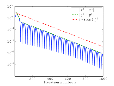
Our main result is that the rate of decay of the error is indeed for a large class of situations that we call standard, in the sense of the following definition.
Definition 1.1.
Consider a basis pursuit problem with solution . Consider an initial value for the Douglas-Rachford iteration, and .
Consider the preimage of the soft thresholding of all vectors with the same signs as :
where
We call a standard problem for the Douglas-Rachford iteration if belongs to the interior of , where is the reflection operator defined earlier. In that case, we also say that the fixed point of is an interior fixed point. Otherwise, we say that is nonstandard for the Douglas-Rachford iteration, and that is a boundary fixed point.
Theorem 1.2.
Consider a standard problem for the Douglas-Rachford iteration, in the sense of the previous definition. Then the Douglas-Rachford iterates obey
where may depend on , and (but not on ), and is the leading principal angle between and .
The auxiliary variable in (1.3) converges linearly for sufficiently large , thus is also bounded by a linearly convergent sequence since .
Intuitively, convergence enters the linear regime when the support of the iterates essentially matches that of . By essentially, we mean that there is some technical consideration (embodied in our definition of a “standard problem”) that this match of supports is not a fluke and will continue to hold for all iterates from and on. When this linear regime is reached, our analysis in the standard case hinges on the simple fact that is a linear transformation on with an eigenvalue of maximal modulus equal to .
In the nonstandard case ( being a boundary fixed point), we furthermore show that the rate of convergence for is generically of the form , where is the leading principal angle between and , with a submatrix of depending on . Nongeneric cases are not a priori excluded by our analysis, but have not been observed in our numerical tests. See Section 2.5 for a discussion of the different types of nonstandard cases.
1.3 Regularized basis pursuit
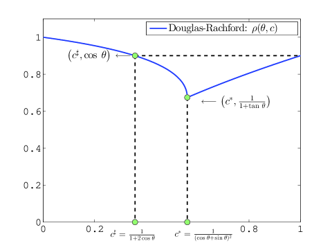
In practice, if is very close to zero, linear convergence with rate might be very slow. The following regularized problem is often used to accelerate convergence,
| (1.4) |
It is proven in [28] that there exists a such that the solution of (1.4) with is the solution of (1.1). See [23] for more discussion of . For the rest of this paper, we assume is taken large enough so that .
For all the discussion regarding -regularized basis pursuit, it is convenient to make the technical assumption that . Notice that regularization is probably unwarranted in the event , since would be a very decent linear convergence rate.
In particular, the Douglas-Rachford splitting (1.2) with and is equivalent to the dual split Bregman method for basis pursuit [27], which will be discussed in Section 4.3.
1.4 Generalized Douglas-Rachford and Peaceman-Rachford
The generalized Douglas-Rachford splitting introduced in [10] can be written as
| (1.5) |
We have the usual DR splitting when . In the limiting case , (1.5) becomes the Peaceman-Rachford (PR) splitting
| (1.6) |
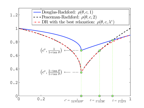
Consider (1.5) with constant relaxation parameter on (1.4). With the same assumptions and notations as in Theorem 1.2, assuming , we have the eventual linear convergence rate where and
For fixed and , the optimal relaxation parameter is
which is a continuous non-increasing function with respect to and has range for .
The convergence rate at the optimal is
See Figure 1.3 for the illustration of the asymptotic linear rate . Several interesting facts can be seen immediately:
1.5 Context
There is neither strong convexity nor Lipschitz continuity in the objective function of (1.1) even locally around , but any with the same support as lies on a low-dimensional manifold, on which the objective function is smooth. Such property is characterized as partial smoothness [24]. In other words, it is not surprising that nonsmooth optimization algorithms for (1.1) converge linearly if has the correct support. For example, see [17, 29].
The main contribution of this paper is the quantification of the asymptotic linear convergence rate for Douglas-Rachford splitting on basis pursuit. It is well-known that Douglas-Rachford on the dual problem is the same as the alternating direction method of multipliers (ADMM) [13], which is also equivalent to split Bregman method [16]. Thus the analysis in this paper also applies to ADMM on the dual problem of -regularized basis pursuit, i.e., the dual split Bregman method for basis pursuit [27]. By analyzing the generalized Douglas-Rachford introduced in [10] including the Peaceman-Rachford splitting, we obtain the explicit dependence of the asymptotic convergence rate on the parameters.
1.6 Contents
Details and proof of the main result will be shown in Section 2. In Sections 3, we apply the same methodology to obtain the asymptotic convergence rates for Douglas-Rachford, generalized Douglas-Rachford and Peaceman-Rachford splittings on the -regularized basis pursuit. In Section 4, we discuss the equivalence between Douglas-Rachford and dual split Bregman method, and their practical relevance. Numerical experiments illustrating the theorems are shown.
2 Douglas-Rachford for Basis Pursuit
2.1 Preliminaries
For any subspace in , we use to denote the orthogonal projection onto of the point
In this section, we denote , , and the resolvents are and . For convenience, we use to denote reflection about , i.e., It is easy to see that is idempotent. Then .
Let denote the set of coordinate indices associated with the nonzero components of , namely, . Recall the definition of in the previous section. Then for any , the soft thresholding operator can be written as .
Lemma 2.1.
The assumption that is the unique minimizer of (1.1) implies .
Proof.
Suppose there exists a nonzero vector . For any with small magnitude, we have and . For nonzero small , the uniqueness of the minimizer implies . Thus .
On the other hand, for the function on a small neighborhood of , the minimum of is , thus . This contradicts with the fact that . ∎
The sum of the dimensions of and should be no larger than since . Thus, implies
also implies the orthogonal complement of the subspace spanned by and is . Therefore, the dimension of is .
2.2 Characterization of the fixed points of
Since , the first order optimality condition for (1.1) reads , thus . Any such is called a dual certificate.
We have the following characterization of the fixed points of .
Lemma 2.2.
The set of the fixed points of can be described as
Moreover, for any two fixed points and , we have . Thus there is a unique fixed point if and only if .
Proof.
For any , consider the vector Since and (implied by ), we have . Further, implies Thus
Second, for any fixed point of the operator , let . Then
| (2.1) |
implies , thus . Further, implies We have , thus
Finally, let and be two fixed points. Then and for some . Notice that implies . So we get . ∎
With the assumption the matrix has full row rank, the following condition is sufficient [12] and necessary [30] to ensure existence of a unique solution to (1.1):
-
1.
those columns of with respect to the support of are linearly independent.
-
2.
there exists a dual certificate such that and .
Therefore, with assumption that there is a unique solution to (1.1), there always exists a dual certificate such that and . By Lemma 2.2, is a fixed point. And is in the interior of since .
We call a fixed point an interior fixed point if is in the interior of the set , or a boundary fixed point otherwise. A boundary fixed point exists only if .
Definition 2.3.
Let and be two subspaces of with . The principal angles () between and are recursively defined by
The vectors and are called principal vectors.
Lemma 2.4.
Assume is a boundary fixed point and lies on a -dimensional face of the set . Namely, there are coordinates such that (). Recall that , hence is a subset of . Let denote the matrix consisting of all row vectors of except . Recursively define as the matrix consisting of all row vectors of except for . If there exists an index such that , let be the smallest such integer; otherwise, let . Then , and the first principal angle between and is nonzero.
Proof.
Let () denote the one dimensional subspaces spanned by , then and .
Let be an interior fixed point. Notice that and for each , thus . By Lemma 2.2 we have , therefore
| (2.2) |
Since , with (2.2), we conclude that
Similarly, we have
Therefore,
| (2.3) |
thus .
Let denote the subspace spanned by and . Since , by(2.3), we have for . Therefore , and the first principal angle between and is nonzero. ∎
2.3 The characterization of the operator
Lemma 2.5.
For any satisfying and any fixed point , where denotes the identity matrix.
Proof.
First, we have
The last step is due to the fact . The definition of fixed points and (2.1) imply
| (2.4) |
thus . So we also have
Let , then
∎
We now study the matrix
| (2.5) |
Let be a matrix whose column vectors form an orthonormal basis of and be a matrix whose column vectors form an orthonormal basis of . Since represents the projection to and so is , we have . Similarly, . Let and be similarly defined for and . The matrix can now be written as
It will be convenient to study the norm of the matrix in terms of principal angles between subspaces.
Without loss of generality, we assume . Let () be the principal angles between the subspaces and . Then the first principal angle since . Let denote the diagonal matrix with the diagonal entries
The singular value decomposition (SVD) of the matrix is with , and the column vectors of and give the principal vectors, see Theorem 1 in [3].
By the definition of SVD, is a matrix and its column vectors are orthonormalized. Let be a matrix whose column vectors are normalized and orthogonal to those of . For the matrix , we have . For the matrix , consider . Since , we have so the SVD of can be written as
| (2.6) |
Notice that , so we have
| (2.9) | |||||
| (2.13) |
Let denote the orthogonal complement of in the subspace , namely, . Then the dimension of is . Let and , then the column vectors of form an orthonormal basis of . The column vectors of are a family of orthonormal vectors in . Moreover, the SVD (2.6) implies the columns of and are principal vectors corresponding to angles between the two subspaces and , see [3]. And implies the largest angle between and is less than , so none of the column vectors of is orthogonal to thus all the column vectors of are in the subspace . By counting the dimension of , we know that column vectors of form an orthonormal basis of .
Let be a whose columns form an orthonormal basis of , then we have
Since is a unitary matrix and , we also have
| (2.15) |
Therefore, we get the decomposition
| (2.23) | |||||
2.4 Standard cases: the interior fixed points
Assume the sequence will converge to an interior fixed point.
First, consider the simple case when , then and the fixed point is unique and interior. Let denote the ball centered at with radius . Let be the largest number such that . Let be the smallest integer such that (thus ). By nonexpansiveness of and , we get for any . By a recursive application of Lemma 2.5, we have
Now, (2.23) and imply . Notice that is normal, so we have for any positive integer . Thus we get the convergence rate for large :
| (2.24) |
If , then there are many fixed points by Lemma 2.2. Let be the set of all interior fixed points. For , let be the largest number such that .
If for some , then consider the Euclidean projection of to , denoted by . Then since for any . By (2.23), is the eigenspace of eigenvalue for the matrix . So we have , thus the error estimate (2.24) still holds.
The sequence may converge to a different fixed points for each initial value ; the fixed point is the projection of to . Here is the smallest integer such that .
2.5 Nonstandard cases: the boundary fixed points
Suppose converges to a boundary fixed point . With the same notations in Lemma 2.4, for simplicity, we only discuss the case . More general cases can be discussed similarly. Without loss of generality, assume and . Then the set is equal to , with . Consider another set . Any neighborhood of intersects both and .
There are three cases:
-
I.
the sequence stays in if is large enough,
-
II.
the sequence stays in if is large enough,
-
III.
for any , there exists such that and .
Case I. Assume converges to and stay in for any . Then must be zero. Otherwise, by (2.23), we have . By (2.23), the eigenspace of associated with the eigenvalue is , so (2.24) still holds.
Case II Assume converges to and stay in for any . Let . Following Lemma 2.5, for any satisfying , we have .
Without loss of generality, assume . Consider the principal angles between and denoted by Let denote the diagonal matrix with diagonal entries Then the matrix can be written as
| (2.25) |
where are redefined accordingly.
Case III Assume converges to and stay in for any . Then . And for we have . Let be the orthogonal complement of in , namely . For , we have and .
For the Case III, which we refer to as nongeneric cases, no convergence results like can be established since whenever . Even though it seems hard to exclude Case III from the analysis, it has not been observed in our numerical tests.
2.6 Generalized Douglas-Rachford
Consider the generalized Douglas-Rachford splitting (1.5) with constant relaxation parameter:
| (2.26) |
Let . Then any fixed point of satisfies , [8]. So the fixed points set of is the same as the fixed points set of . Moreover, for any satisfying and any fixed point , .
To find the asymptotic convergence rate of (2.26), it suffices to consider the matrix . By (2.23), we have
where .
Notice that is a normal matrix. By the discussion in Section 2, if in the iteration of (2.26) converges to an interior fixed point, the asymptotic convergence rate will be governed by the matrix
Note that for any . Therefore, the asymptotic convergence rate of (2.26) is always slower than (1.3) if . We emphasize that this does not mean (1.3) is more efficient than (2.26) for to reach a given accuracy.
2.7 Relation to the Restricted Isometry Property
Let be a random matrix and each column of is normalized, i.e., for each . The Restricted Isometry Property (RIP) introduced in [5] is as follows.
Definition 2.7.
For each integer the restricted isometry constants of is the smallest number such that
| (2.27) |
holds for all vectors with at most nonzero entries.
In particular, any vector with the same support as can be denoted as for some . The RIP (2.27) with implies
Let denote the smallest eigenvalue of . Then since we assume has full row rank. For any vector , we have
where the last step is due to the Courant–Fischer–Weyl min-max principle.
Therefore, we get
| (2.28) |
We will show that (2.28) gives a lower bound of the first principal angle between two subspaces and . Notice that (2.15) implies
by which we have
Let . Since , (2.28) is equivalent to
which implies by the Courant–Fischer–Weyl min-max principle. So the RIP constant gives us
2.8 Numerical examples
We consider several examples for (1.3). In all the examples, unless specified otherwise. For examples in this subsection, the angles between the null spaces can be computed by singular value decomposition (SVD) of [3].
Example 1 The matrix is a random matrix with standard normal distribution and has three nonzero components. By counting dimensions, we know that . Therefore there is only one fixed point. See Figure 1.1 for the error curve of and with . Obviously, the error is not monotonically decreasing but is since the operator is non-expansive. And the slope of is exactly for large .
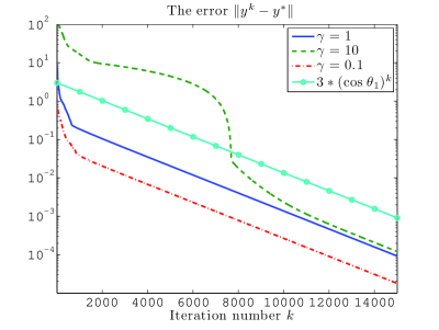
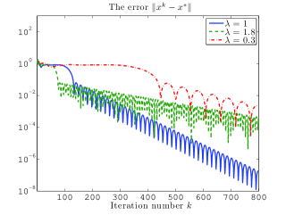
Example 2 The matrix is a random matrix with standard normal distribution and has ten nonzero components. Thus there is only one fixed point. See Figure 2.1 for the error curve of with . We take as the result of (1.3) after iterations. The slopes of for different are exactly for large .
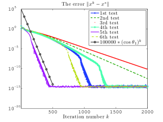
Example 3 The matrix is a submatrix of a Fourier matrix and has two nonzero components. There are interior and boundary fixed points. In this example, we fix and test (1.3) with random for six times. See Figure 2.2 for the error curve of . In Figure 2.2, in four tests, converges to an interior fix point, thus the convergence rate for large is governed by . In the second and third tests, converges to different boundary fixed points111At least, numerically so in double precision. thus convergence rates are slower than . Nonetheless, the rate for large is still linear.
Example 4 The matrix is a random matrix with standard normal distribution and has three nonzero components. See Figure 2.3 for the comparison of (1.3) and (2.26) with .
Remark 2.8.
To apply Douglas-Rachford splitting (1.2) to basis pursuit (1.1), we can also choose and , then Douglas-Rachford iterations become
| (2.29) |
The discussion in this section can be applied to (2.29). In particular, the corresponding matrix in (2.5) is , thus all the asymptotic convergence rates remain valid. For all the numerical tests in this paper, we did not observe any significant difference in performance between (1.3) and (2.29).
3 The regularized Basis Pursuit
3.1 Preliminaries
For the regularized Basis Pursuit (1.4), to use Douglas-Rachford splitting (1.2) to solve the equivalent problem , there are quite a few splitting choices:
-
1.
(3.1) -
2.
(3.2)
The following two resolvents will be needed:
-
•
, .
-
•
,
3.2 Douglas-Rachford splitting
In particular, Douglas-Rachford splitting (1.2) using (3.1) with and is equivalent to the dual split Bregman method [27]. See Section 4.3 for the equivalence. We first discuss this special case.
Since is a strongly convex function, (1.4) always has a unique minimizer as long as is nonempty. The first order optimality condition implies the dual certificate set is nonempty. Let .
Lemma 3.1.
The set of the fixed points of can be described as
The proof is similar to the one of Lemma 2.2. We also have
Lemma 3.2.
For any satisfying and any fixed point , where .
Proof.
First, we have
Similarly we also have
Let , then
∎
Consider the matrix
| (3.4) |
Then where .
Following the proof in [30], it is straightforward to show there exists a dual certificate such that and . So there is at least one interior fixed point. Following Lemma 2.2, there is only one fixed point if and only if .
For simplicity, we only discuss the interior fixed point case. The boundary fixed point case is similar to the previous discussion.
Assume converges to an interior fixed point . Let be the largest number such that . Let be the smallest integer such that (thus ). By nonexpansiveness of and , we get for any . So we have
Notice that is a nonnormal matrix, so is much less than for large . Thus the asymptotic convergence rate is governed by , which is equal to the norm of the eigenvalues of with the largest magnitude.
It suffices to study the matrix because (otherwise cannot converge to ).
Notice that . Let denote the magnitude of the solution with the largest magnitude for the quadratic equation , with discriminant .
The two solutions of are . Notice that for and , we have
| (3.6) |
It is straightforward to check that is monotonically decreasing with respect to for . Therefore, the asymptotic convergence rate is equal to if .
Let which is equal to . Let which is the solution to . See Figure 1.2. Then for any , we have . Namely, the asymptotic convergence rate of (3.3) is faster than (1.3) if . The best asymptotic convergence rate that (3.3) can achieve is when .
Remark 3.3.
The general cases of the two alternatives (3.1) and (3.2) with any and can be discussed similarly. For Douglas-Rachford splitting (1.2) using (3.1) with and (3.2) with or , the asymptotic linear rate (3.6) holds. Compared to (3.3), we observed no improvement in numerical performance by using (3.1) or (3.2) with any other values of and in all our numerical tests.
3.3 Generalized Douglas-Rachford and Peaceman-Rachford splittings
For the generalized Douglas-Rachford splitting (1.5), the choice of and in the (3.1) and (3.2) may result in different performance. The main difference can be seen in the limiting case , for which (1.5) becomes the Peaceman-Rachford splitting (1.6).
If is convex and is strongly convex, the convergence of (1.6) is guaranteed, see [9, 18]. On the other hand, (1.5) may not converge if is only convex rather than strongly convex. For instance, (1.6) with (3.1) and (or (3.2) and ) did not converge for examples in Section 4.4. To this end, the best choices of and for (1.5) should be (3.1) with and (3.2) with . We only discuss the case of using (3.1) with . The analysis will hold for the other one.
Let and . Consider the following generalized Douglas-Rachford splitting with a constant relaxation parameter :
| (3.7) |
It suffices to study the matrix . Notice that . Let denote the magnitude of the solution with the largest magnitude for the quadratic equation , with discriminant .
The two solutions of are . Notice that for and , we have
| (3.9) |
It is straightforward to check that and is monotonically decreasing with respect to for . Therefore, the asymptotic convergence rate of (3.7) is governed by if .
The next step is to evaluate . When , is monotonically decreasing with respect to . Let , for the quadratic equation , we have
Let , then
| (3.10) |
which is a continuous non-increasing function w.r.t and has range for .
The convergence rate with is
See Figure 1.3 for the illustration of the asymptotic linear rate .
Remark 3.4.
We emphasize several interesting facts:
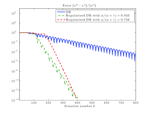
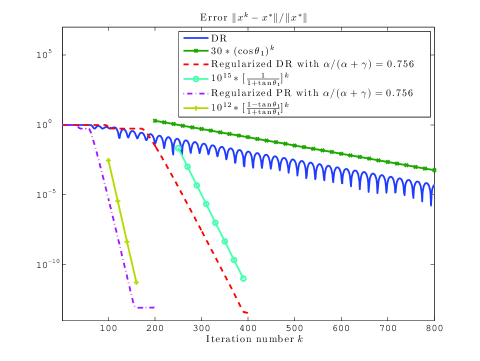
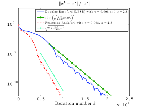
Example 5 The matrix is a random matrix with standard normal distribution and has two nonzero components. We test the algorithms (3.3) and (3.7). See Section 4.3 for the equivalence between (3.3) and the dual split Bregman method in [27]. See Figure 3.1 for the error curve of . The best choice of the parameter according to Figure 1.2 should be , which is for this example. Here indeed gives the best asymptotic rate for (3.3) but is not necessarily the most efficient choice for a given accuracy, as we can see in the Figure 1.2 (a). The best asymptotic rates (3.3) and (3.7) are and respectively when as we can see in Figure 3.1 (b).
4 Dual interpretation
4.1 Chambolle and Pock’s primal dual algorithm
The algorithm (1.2) is equivalent to a special case of Chambolle and Pock’s primal-dual algorithm [6]. Let , then (1.2) with and is equivalent to
| (4.1) |
where is the conjugate function of . Its resolvent can be evaluated by the Moreau’s identity,
Let and , then the duality gap of the point converges with the rate . See [6] for the proof. If and , then will converge to a dual certificate .
4.2 Alternating direction method of multipliers
In this subsection we recall the the widely used alternating direction method of multipliers (ADMM), which serves as a preliminary for the next subsection. ADMM [15, 14] was shown in [13] to be equivalent to the Douglas-Rachford splitting on the dual problem. To be more specific, consider
| (P) |
where and are convex functions and is a matrix. The dual problem of the equivalent constrained form is
| (D) |
By applying the Douglas-Rachford splitting (1.2) on and , one recovers the classical ADMM algorithm for (P),
| (ADMM) |
with the change of variable , and unchanged.
After its discovery, ADMM has been regarded as a special augmented Lagrangian method. It turns out that ADMM can also be interpreted in the context of Bregman iterations. The split Bregman method [16] for (P) is exactly the same as (ADMM), see [26]. Since we are interested in Douglas-Rachford splitting for the primal formulation of the minimization, the algorithms analyzed in the previous sections are equivalent to ADMM or split Bregman method applied to the dual formulation.
4.3 Split Bregman method on the dual problem
In this subsection we show that the analysis in Section 3 can also be applied to the split Bregman method on the dual formulation [27]. The dual problem of regularized basis pursuit (1.4) can be written as
| (4.2) |
where denotes the dual variable, see [28].
By switching the first two lines in (ADMM), we get a slightly different version of ADMM:
| (ADMM2) |
The well-known equivalence between (ADMM) and Douglas-Rachford splitting was first explained in [13]. See also [26, 11]. For completeness, we discuss the equivalence between (ADMM2) and Douglas-Rachford splitting.
Theorem 4.1.
Proof.
It is straightforward to check that and . By Theorem 4.1, (LB-SB) is exactly the same as (3.3). Therefore, all the results in Section 3 hold for (LB-SB). In particular, the dependence of the eventual linear convergence rate of (LB-SB) on the parameters is governed by (3.6) as illustrated in Figure 1.2.
Remark 4.2.
Let be the minimizer of (4.2) then is the solution to (1.4), see [28]. So can be used as the approximation to , the solution to (1.4), as suggested in [27]. By Theorem 4.1, we can see that will converge to too. And it is easy to see that satisfies the constraint in (3.3). But does not necessarily lie in the affine set . Thus and are two completely different sequences even though they both can be used in practice.
4.4 Practical relevance
To implement the algorithm exactly as presented earlier, the availability of is necessary. Algorithms such as (1.3) and (3.3), the same as (LB-SB), are not suitable if is prohibitive to obtain. On the other hand, there are quite a few important problems for which is cheap to compute and store in memory. For instance, may be relatively small and is a well-conditioned matrix in typical compressive sensing problems. Another example is when represents a tight frame transform, for which is the identity matrix.
As for the efficiency of (LB-SB), see [27] for the comparison of (LB-SB) with other state-of-the-art algorithms.
Next, we discuss several examples of (3.3), (LB-SB) and (3.7) for the tight frame of discrete curvelets [4], in the scope of an application to interpolation of 2D seismic data. In the following examples, let denote the matrix representing the wrapping version of the two-dimensional fast discrete curvelet transform [4], then represents the inverse curvelet transform and is the identity matrix since the curvelet transform is a tight frame.
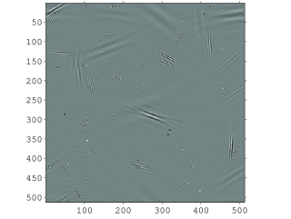
Example 6 We construct an example with to validate formula (3.6). Consider a random sparse vector with length and nonzero entries, in the curvelet domain which is the range of the curvelet transform of images. The size of the abstract matrix is . Notice that, for any , is implemented through fast Fourier transform, thus the explicit matrix representation of is never used in computation. Let denote the image generated by taking the inverse transform of , see Figure 4.1 (a).
Suppose only the data is given, to recover a sparse curvelet coefficient, we can solve (1.1) with and being vectors in curvelet domain.
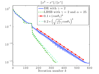
We use both (1.3) and (3.3) with and to solve (1.1). Since is a huge implicitly defined matrix, it is not straightforward to compute the angles exactly by SVD as in small matrices examples. Instead, we obtain approximately the first principal angle between and in a more efficient ad hoc way in Appendix B. Assuming and , if in (3.3) converged to a fixed point of the same type (interior or boundary fixed point) as in (1.3), the eventual linear rate of (3.3) should be by (3.6). As we can see in Figure 4.1 (b), the error curve for (3.3) matched well with the eventual linear rate .
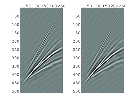
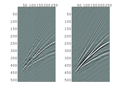
Example 7 In this example, we consider a more realistic data as shown in the left panel of Figure 4.2 (a). The data is generated by the following procedure. First, take a synthetic seismic dataset consisting of traces (columns) and time samples (rows). Second, solve the basis pursuit with by (3.3) up to iterations. Third, set the entries in smaller than to zero and let denote the resulting sparse vector, which has nonzero entries. Finally, set .
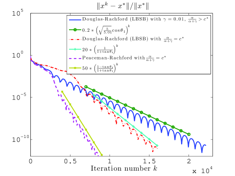
Given only the data , the direct curvelet transform is not as sparse as . Thus is not the most effective choice to compress the data. To recover the curvelet coefficient sequence , we alternatively solve (1.1) with and being vectors in curvelet domain. For this particular example, is recovered. By the method in Appendix B, we get . To achieve the best asymptotic rate, the parameter ratio should be by (3.6). See Figure 4.2 (b) for the performance of (LB-SB) and (3.7) with fixed and we can see the asymptotic linear rates match the best rates and when .
Example 8 We consider an example of seismic data interpolation via curvelets. Let be the same data as in the previous example, see the left panel in Figure 4.2 (a). Let be the sampling operator corresponding to percent random traces missing, see Figure 4.3 (a).
Given the observed data , to interpolate and recover missing data (traces), one effective model is to pursue sparsity in the curvelet domain [21], i.e., solving with the constraint . Here is a vector of curvelet coefficients. If is a minimizer, then can be used as the recovered data. Let . Then since represents a sampling operator. Thus (3.3) and (LB-SB) are straightforward to implement. For this relatively ideal example, the original data can be recovered. We also observe the eventual linear convergence. See Figure 4.3 (a) for the recovered data after iterations of (3.3) and (LB-SB).
5 Conclusion
In this paper, we analyze the asymptotic convergence rate for Douglas-Rachford splitting algorithms on the primal formulation of the basis pursuit, providing a quantification of asymptotic convergence rate of such algorithms. In particular, we get the asymptotic convergence rates for -regularized Douglas-Rachford, and the generalized Douglas-Rachford including the Peaceman-Rachford splitting. The explicit dependence of the convergence rate on the parameters may shed light on how to choose parameters in practice.
Appendix A
Lemma A.1.
Let be a firmly non-expansive operator, i.e., for any and . Then the iterates satisfy where is any fixed point of .
Proof.
The firm non-expansiveness implies
Let and , then
Summing the inequality above, we get . By the firm non-expansiveness and the Cauchy-Schwarz inequality, we have which implies . ∎
For the Douglas-Rachford splitting, see [20] for a different proof for this fact.
Appendix B
Suppose , we discuss an ad hoc way to find an approximation of the first principal angle between and . Define the projection operators and . Consider finding a point in the intersections of two linear subspaces,
| (B.1) |
by von Neumann’s alternating projection algorithm,
| (B.2) |
or the Douglas-Rachford splitting,
| (B.3) |
Notice that is the only solution to (B.1). By fitting lines to for large in (B.2) and (B.3), we get an approximation of and respectively. In practice, (B.2) is better since the rate is faster and is monotone in . This could be an efficient ad hoc way to obtain when the matrix is implicitly defined as in the examples in Section 4.4.
References
- [1] Francisco J. Aragón Artacho and Jonathan M. Borwein. Global convergence of a non-convex Douglas-Rachford iteration. Journal of Global Optimization, pages 1–17, 2012.
- [2] Heinz H. Bauschke, Patrick L. Combettes, and D. Russell Luke. Phase retrieval, error reduction algorithm, and fienup variants: a view from convex optimization. J. Opt. Soc. Am. A, 19(7):1334–1345, Jul 2002.
- [3] Åke Björck and Gene H. Golub. Numerical Methods for Computing Angles Between Linear Subspaces. Mathematics of Computation, 27(123), 1973.
- [4] E. Candès, L. Demanet, D. Donoho, and L. Ying. Fast discrete curvelet transforms. Multiscale Modeling Simulation, 5(3):861–899, 2006.
- [5] E.J. Candès and T. Tao. Decoding by linear programming. Information Theory, IEEE Transactions on, 51(12):4203 – 4215, dec. 2005.
- [6] Antonin Chambolle and Thomas Pock. A first-order primal-dual algorithm for convex problems with applications to imaging. J. Math. Imaging Vis., 40(1):120–145, May 2011.
- [7] Scott Shaobing Chen, David L. Donoho, Michael, and A. Saunders. Atomic decomposition by basis pursuit. SIAM Journal on Scientific Computing, 20:33–61, 1998.
- [8] Patrick L. Combettes. Solving monotone inclusions via compositions of nonexpansive averaged operators. Optimization, 53:475–504, 2004.
- [9] Patrick L Combettes. Iterative construction of the resolvent of a sum of maximal monotone operators. J. Convex Anal, 16(4):727–748, 2009.
- [10] Jonathan Eckstein and Dimitri P. Bertsekas. On the Douglas-Rachford splitting method and the proximal point algorithm for maximal monotone operators. Mathematical Programming, 55:293–318, 1992.
- [11] E. Esser. Applications of Lagrangian based alternating direction methods and connections to split Bregman. CAM Report 09-31, UCLA, 2009.
- [12] J.-J. Fuchs. On sparse representations in arbitrary redundant bases. Information Theory, IEEE Transactions on, 50(6):1341 – 1344, june 2004.
- [13] D. Gabay. Applications of the method of multipliers to variational inequalities. Augmented Lagrangian Methods: Applications to the Solution of Boundary-Value Problems edited by M. FORTIN and R. GLOWINSKI, 1983.
- [14] D. Gabay and B. Mercier. A dual algorithm for the solution of nonlinear variational problems via finite element approximation. Comput. Math. Appl., 2(1):17–40, January 1976.
- [15] R. Glowinski and A. Marroco. Sur l’approximation, par elements finis d’ordre un, et la resolution, par penalisation-dualité d’une classe de problemes de dirichlet non lineares. Revue Française d’Automatique, Informatique et Recherche Opérationelle, 9:41–76, 1975.
- [16] Tom Goldstein and Stanley Osher. The split Bregman method for L1-regularized problems. SIAM J. Img. Sci., 2(2):323–343, April 2009.
- [17] Elaine T Hale, Wotao Yin, and Yin Zhang. Fixed-point continuation for ell_1-minimization: Methodology and convergence. SIAM Journal on Optimization, 19(3):1107–1130, 2008.
- [18] Deren Han and Xiaoming Yuan. Convergence analysis of the peaceman-rachford splitting method for nonsmooth convex optimization. 2012.
- [19] B. He and X. Yuan. On the O convergence rate of the Douglas–Rachford alternating direction method. SIAM Journal on Numerical Analysis, 50(2):700–709, 2012.
- [20] Bingsheng He and Xiaoming Yuan. On non-ergodic convergence rate of Douglas-Rachford alternating direction method of multipliers. preprint, 2012.
- [21] Felix J. Herrmann and Gilles Hennenfent. Non-parametric seismic data recovery with curvelet frames. Geophysical Journal International, 173(1):233–248, 2008.
- [22] Robert Hesse and D. Russell Luke. Nonconvex notions of regularity and convergence of fundamental algorithms for feasibility problems. preprint.
- [23] M.-J. Lai and W. Yin. Augmented l1 and nuclear-norm models with a globally linearly convergent algorithm. Technical report, Rice University CAAM, 2012.
- [24] A. S. Lewis. Active sets, nonsmoothness, and sensitivity. SIAM J. on Optimization, 13(3):702–725, August 2002.
- [25] P. L. Lions and B. Mercier. Splitting algorithms for the sum of two nonlinear operators. SIAM J. Numer. Anal., 16:964–979, 1979.
- [26] Simon Setzer. Split Bregman algorithm, Douglas-Rachford splitting and frame shrinkage. In Proceedings of the Second International Conference on Scale Space and Variational Methods in Computer Vision, SSVM ’09, pages 464–476, Berlin, Heidelberg, 2009. Springer-Verlag.
- [27] Yi Yang, Michael Moller, and Stanley Osher. A dual split Bregman method for fast minimization. Mathematics of Computation, to appear.
- [28] Wotao Yin. Analysis and generalizations of the linearized Bregman method. SIAM J. Img. Sci., 3(4):856–877, October 2010.
- [29] Wotao Yin and Stanley Osher. Error forgetting of bregman iteration. Journal of Scientific Computing, 54(2-3):684–695, 2013.
- [30] Hui Zhang, Wotao Yin, and Lizhi Cheng. Necessary and sufficient conditions of solution uniqueness in 1 minimization. Technical report, Rice University CAAM, 2012.
