Stellar Populations in the Central 0.5 pc of the Galaxy II: The Initial Mass Function

Abstract

The supermassive black hole at the center of the Milky Way plays host to a massive, young cluster that may have formed in one of the most inhospitable environments in the Galaxy. We present new measurements of the global properties of this cluster, including the initial mass function (IMF), age, and cluster mass. These results are based on Keck laser-guide-star adaptive optics observations used to identify the young stars and measure their Kp-band luminosity function as presented in Do et al. (2012). A Bayesian inference methodology is developed to simultaneously fit the global properties of the cluster utilizing the observations and extensive simulations of synthetic star clusters. We find that the slope of the mass function for this cluster is $\alpha=1.7\pm 0.2$, which is steeper than previously reported, but still flatter than the traditional Salpeter slope of $2.35$. The age of the cluster is between 2.5-5.8 Myr with 95% confidence, which is a younger age than typically adopted but consistent within the uncertainties of past measurements. The exact age of the cluster is difficult to determine since our results show two distinct age solutions (3.9 Myr and 2.8 Myr) due to model degeneracies in the relative number of Wolf-Rayet and OB stars. The total cluster mass is between 14,000 - 37,000 M_⊙ above 1 M_⊙ and it is necessary to include multiple star systems in order to fit the observed luminosity function and the number of observed Wolf-Rayet stars. The new IMF slope measurement is now consistent with X-ray observations indicating a factor of 10 fewer X-ray emitting pre-main-sequence stars than expected when compared with a Salpeter IMF. The young cluster at the Galactic center is one of the few definitive examples of an IMF that deviates significantly from the near-universal IMFs found in the solar neighborhood.

1. Introduction

Young nuclear star clusters have now been found surrounding supermassive black holes in a number of nearby galaxies (e.g. Lauer et al., 1998; Bender et al., 2005; Seth et al., 2006). The best studied young nuclear cluster is at the center of our own Milky Way Galaxy, located only 8 kpc away and surrounding a supermassive black hole (SMBH) of mass M$\sim 4\times 10^{6}$ M_⊙ (Eckart & Genzel, 1997; Ghez et al., 1998, 2000, 2003, 2005, 2008; Genzel et al., 2000; Schödel et al., 2002, 2003; Eisenhauer et al., 2005; Gillessen et al., 2009a). The young stars are located within 1 pc of the SMBH and are thought to have formed as recently as 4-8 Myr ago (Paumard et al., 2006). The origin of the young stars, in such close proximity to the supermassive black hole, is puzzling, given that the strong tidal forces in this region will shear apart typical molecular clouds before they can collapse to form stars. Thus, the young nuclear cluster (YNC) is a key laboratory for understanding whether and how stars form under such extreme conditions.

The YNC at the Galactic center has several observed properties that may help to determine its origin. To date, more than 100 young stars have been spectroscopically identified as OB supergiants, Wolf-Rayet stars, and, more recently, OB main-sequence stars (Allen et al., 1990; Krabbe et al., 1991; Blum et al., 1995; Krabbe et al., 1995; Tamblyn et al., 1996; Najarro et al., 1997; Ghez et al., 2003; Paumard et al., 2006; Bartko et al., 2010; Do et al., 2012). The young population appears to fall into three dynamical categories; (1) a well-defined clockwise rotating disk ranging from 0.03 pc to at least 0.5 pc with moderate eccentricities, (2) an off-the-disk population in a more isotropic distribution over the same distances and also with moderate eccentricities, and (3) $\sim$10% cluster within 0.03 pc of the black hole with high eccentricities of $\bar{e}=0.8$ (Genzel et al., 2000; Levin & Beloborodov, 2003; Genzel et al., 2003; Paumard et al., 2006; Ghez et al., 2008; Lu et al., 2009; Gillessen et al., 2009b; Yelda, 2012). These kinematic differences have led to some speculation that the young stars may have been formed in multiple episodes, although the outer two groups (#1 and #2) have consistent stellar populations (Paumard et al., 2006). The inner group (#3) was most likely dynamically injected, since the SMBH’s tidal forces are too strong to permit star formation at these close distances. Initial theories suggested that this inner population was substantially older, as long times were needed to scatter inward a large number of binary systems that can interact with the SMBH and leave behind a star on a highly eccentric orbit with a small semi-major axis (e.g. Brown et al., 2007; Perets et al., 2007). However, more recent inclusion of additional dynamical effects suggests that the stars in the central region can be brought in more efficiently than initially thought (Löckmann et al., 2009; Madigan et al., 2011). Thus, it remains uncertain whether the inner group of young stars was originally part of the outer groups and born in the same star formation event. In the outer groups, there is some observational support for a possible warp in the clockwise disk (Bartko et al., 2009), a second face-on disk made of counter-clockwise rotating stars (Genzel et al., 2003; Bartko et al., 2009), and for sub-clusters of stars both on and off the disk (Maillard et al., 2004; Schödel et al., 2005; Lu et al., 2005), although the statistical significance of these results is still debated (Lu et al., 2009; Yelda, 2012). The total surface density profile of the young stars in the plane of the sky is $\Sigma\propto R^{-1}$ (Do et al., 2012) and substantially steeper in the disk plane $\Sigma_{\textrm{CW disk}}\propto R^{-2}$. Early analysis of the bright stars (K$\leq$13) gave an age for the cluster of 6 $\pm$ 2 Myr based on the presence of Wolf-Rayet (WR) stars and the proportions of WR stars to O stars (Paumard et al., 2006). In this same work, the observed number of WR and O stars and their luminosity function suggested that the the total cluster mass is $10^{4}$ M_⊙ and the initial mass function (IMF, $dN/dm\propto m^{\alpha}$) is top-heavy with a slope significantly flatter than Salpeter (1955, $\alpha=2.35$). However, these results were limited by the lack of sensitivity to less massive, main-sequence stars (K$>$13, M$<$20 M_⊙ ). Deeper spectroscopic studies initially showed that the luminosity function for the young stars appears to have a sharp turn-over at K$=$13.5, suggesting that the present-day mass function is extremely top-heavy with a slope of $\alpha=0.45\pm 0.3$ (Bartko et al., 2010). A top-heavy IMF is also supported by the Chandra X-ray observations of the region, given that lower mass young stars should still be coronally active and emitting copious X-rays that aren’t detected (Nayakshin & Sunyaev, 2005).

Several possible models for the origin of the young stars have been proposed and the two presently supported by observations include (1) formation in situ in a massive self-gravitating molecular disk (Levin & Beloborodov, 2003) or (2) disruption of an in-falling massive cluster formed much further away (Gerhard, 2001). In situ formation models invoke the build-up of a gas disk surrounding the SMBH that reached a critical mass ($\sim 10^{4}$ M_⊙ ) approximately 6 Myr ago such that local self-gravity within the disk became sufficient to overcome the tidal shear, the disk collapsed along the vertical direction and formed stars (Levin & Beloborodov, 2003; Kolykhalov & Syunyaev, 1980; Shlosman & Begelman, 1989; Morris & Serabyn, 1996; Sanders, 1998; Goodman, 2003; Nayakshin & Cuadra, 2005). If such a disk was built up slowly, the gas and resulting young stars would largely be on circular orbits, which does not appear to be the case observationally (Lu et al., 2009; Bartko et al., 2009). Modified in situ formation models include the rapid infall of a single massive molecular cloud or the collision of two in-falling clouds to produce non-circular orbits and the on-disk and off-disk populations (Alexander et al., 2007; Cuadra et al., 2008; Sanders, 1998; Vollmer & Duschl, 2001; Nayakshin et al., 2007; Hobbs & Nayakshin, 2009). The surface density of stars formed in situ in a slowly-built gas disk may be steep ($\Sigma\propto R^{-2}$); however, the surface density resulting from a cloud-cloud collision is less well constrained. For in-falling cluster scenarios, the young stars are formed a few parsecs away in a massive young star cluster that spirals in via dynamical friction and disrupts in the central parsec (Gerhard, 2001). In order for such a cluster to migrate into the central parsec within only a few million years, the cluster must be very massive and centrally concentrated and perhaps even host an intermediate mass black hole (IMBH) at its center (Kim & Morris, 2003; Portegies Zwart et al., 2003; McMillan & Portegies Zwart, 2003; Gürkan & Rasio, 2005; Hansen & Milosavljević, 2003; Kim et al., 2004). Such a scenario would produce the on-disk population and a flatter surface density profile ($\Sigma\propto R^{-0.75}$), with the off-disk population resulting from subsequent dynamical perturbations (Haas et al., 2011; Baruteau et al., 2011). In situ formation models are favored based on the density profiles and available time scales; however, no single model completely explains all of the observed properties. One important prediction of current in situ formation models is that the initial mass function should be very top-heavy due to the extreme temperatures, pressures, densities, and ambient radiation fields present in the central parsec (Nayakshin et al., 2006; Nayakshin, 2006; Alexander et al., 2007, 2008; Cuadra et al., 2008). However, a number of model parameters are still very uncertain (e.g. gas infall rate, temperature, pressure, and cooling time) and a wide variety of initial mass functions are still possible.

The initial mass function, age, and mass of the young nuclear star cluster at the Galactic center is of particular interest both for understanding the origin of the young stars and exploring star formation under extreme conditions. Past observations of a turn-over in the near-infrared luminosity function and the low total X-ray emission apparently support a top-heavy IMF. However, new observations presented in our companion paper, Do et al. (2012, Paper I), show a luminosity function that does not turn over, but continues to rise; warranting a new analysis of the mass function.

In this work, we compare the near-infrared photometry of the spectroscopically identified young stars in Paper I to models of star clusters in order to determine the age, mass function, and total mass of the young nuclear star cluster. Details on the observational sample and measurements are presented in §2. Synthetic clusters are generated using stellar evolution and atmosphere models to produce individual stars as they would appear at the Galactic center in §3.1. In §3.2 we present a Bayesian inference method for fitting the observed data with synthetic clusters to determine the cluster’s properties and uncertainties. Results in §4 show that the present-day mass function is slightly flatter than a Salpeter IMF and rule out a mass function as top-heavy as previously claimed. We also find a younger age and our modeling requires the inclusion of binaries and multiple star systems to adequately fit the luminosity function.

2. Observed Data & Sample

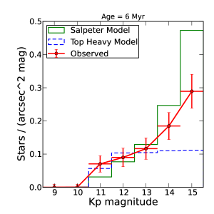
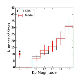
Observations and data used in this paper are described in Paper I. Our data sample includes all stars with a non-zero probability of being a young, early-type star ($p_{yng}>0$). For each star, the measurements consist of a Kp magnitude corrected for differential extinction (K${}^{\prime}_{\Delta A}$), a Kp uncertainty ($\sigma_{K^{\prime}}$), the probability of youth ($p_{yng}$), and an indicator for whether the star is a Wolf-Rayet star. Only stars with K${}^{\prime}_{\Delta A}\leq 15.5$ are included. The modeling presented in this work utilizes these individual measurements rather than a binned Kp luminosity function (KLF). However for illustrative purposes, Figure 1 shows our binned KLF compared with a model KLF for a cluster with an age of 6 Myr, extinction of A${}_{Ks}=2.7$, distance of 8 kpc, and an IMF slope of $\alpha=0.45$, consistent with previously published best-fit cluster parameters (Bartko et al., 2010). The discrepancy between our observed KLF and this model motivates the work presented below as we attempt to derive new best-fit cluster parameters and uncertainties.

In our sample, we have chosen to include young stars at all radii, including the central 0$\farcs$8 region immediately around the supermassive black hole. There are some suggestions that the stars in this central region were not formed in the most recent starburst, but rather in an earlier event. The brightest early-type star in this region, S0-2, is a B0-B2.5 V star with an age of less than 15 Myr based on its measured temperature, gravity, and luminosity (Martins et al., 2008). The other early-type stars in this region have spectral features consistent with main-sequence stars (Eisenhauer et al., 2005) and the oldest age for a main-sequence star at Kp$=$15.5 (A${}_{Ks}=2.7$, d$=$8 kpc) is less than 20 Myr. Given these age constraints and the large uncertainties in the theoretical scattering efficiencies, it remains plausible that the young stars in the central region of our sample are the same age as the stars at larger radii. Furthermore, as described in Paper I, including or discarding the stars within a radius of 0$\farcs$8 does not significantly change the shape of the KLF.

Figure 1.— The observed Kp luminosity function (KLF) for early-type stars in the Galactic center nuclear cluster (Paper I) compared with previously proposed model KLFs. The observed Kp magnitudes (red) are corrected for differential extinction to a common extinction value of A${}_{Ks}=2.7$. A model KLF is shown for published best-fitting cluster parameters (blue) with an IMF slope of $\alpha=0.45$, age of 6 Myr, and a distance of 8 kpc (Bartko et al., 2010). For comparison, a model KLF is also shown for a similar cluster with a Salpeter IMF slope of $\alpha=2.35$ (green).

3. Modeling the Observed Cluster

While the early-type stellar population in the central parsec of the Galaxy can be divided into several different kinematic sub-groups (Paumard et al., 2006; Ghez et al., 2008; Lu et al., 2009; Bartko et al., 2009; Gillessen et al., 2009b), it is not yet clear whether these sub-groups have different origins, or whether all the young stars formed from the same starburst and were differentiated via subsequent dynamical processes. Therefore, we choose to analyze the entire population of young stars as a single starburst cluster and to estimate the cluster’s mass function, age, and total mass.

The traditional approach to deriving a mass function would be to construct a binned KLF from the observed Kp magnitudes, assume a distance and extinction, and use a mass-luminosity relation from models of stellar evolution and atmospheres to convert from observed magnitudes to initial stellar masses. This approach has several shortcomings, including arbitrarily choosing bin sizes, neglecting uncertainties on stellar brightness, not accounting for multiple systems, and correlations in the cluster age, mass, and IMF (Maíz Apellániz & Úbeda, 2005; Maíz Apellániz, 2008; Maíz-Apellániz, 2009). More recent and rigorous statistical methods, particularly those using Bayesian inference, provide flexibility and produce robust estimates of the most probable cluster parameters and their uncertainties (e.g. Allen et al., 2005). We have developed a Bayesian inference methodology for deriving the physical properties of an observed young star cluster using simulations of synthetic clusters. The process of simulating a synthetic young cluster is described in §3.1 and the full Bayesian methodology, implementation, and testing is described in §3.2, §3.3, and §3.4, respectively. Readers wishing to skip the detailed description of the modeling may proceed to §4 where the resulting best-fit cluster properties and uncertainties are presented.

3.1. Synthetic Clusters

Model young star clusters are produced assuming an instantaneous starburst at time $t$, at distance $d$, with an observed cluster mass $M_{cl,obs}$. The initial mass function of the cluster is described as a single power-law given by the probability density function

$$\frac{dN}{dm}\propto p(m) = \frac{(1-\alpha)m^{-\alpha}}{m_{max}^{1-\alpha}-m_{min}^{1-\alpha}}\quad[\alpha\neq 1]$$ (1)

$$= \frac{m^{-\alpha}}{\ln m_{max}-\ln m_{min}}\quad[\alpha=1]$$ (2)

where $\alpha$ is allowed to vary and has the value $\alpha=2.35$ in the case of a typical IMF for the high-mass end of a solar-neighborhood population (Salpeter, 1955). In addition to these free parameters, a number of fixed parameters are also needed to fully model the cluster. First, the extinction is fixed to A${}_{Ks}=2.7$ as we will compare to observations that have been corrected for differential extinction to this value. The metallicity is fixed to Z=0.02, which is roughly solar. Observations suggest the young GC population is consistent with solar iron abundance; but may be as high as 2$\times$ solar and seems enhanced in $\alpha$-elements (Carr et al., 2000; Ramírez et al., 2000; Najarro et al., 2004; Cunha et al., 2007; Martins et al., 2008). The choice to keep metallicity fixed to solar is also motivated by the lack of complete stellar evolution and atmosphere models at other metallicities and abundance ratios. Section 5 discusses possible uncertainties associated with restricting our analysis to solar metallicity. The range of masses we consider is set as $m_{min}$ = 1 M_⊙ and $m_{max}$ = 150 M_⊙ and is kept fixed throughout the analysis. This is justified as our observations do not include stars below 10 M_⊙ due to sensitivity limits and stars above 150 M_⊙ have already exploded for clusters older than 3 Myr. Thus the currently observed stars have no power to constrain the low or high mass cutoffs and a more expansive mass range would not impact our results. For each star drawn from the IMF, we must also consider whether it has companions (Sagar & Richtler, 1991; Kroupa, 1995; Goodwin & Kroupa, 2005; Thies & Kroupa, 2007; Maíz-Apellániz, 2009; Weidner et al., 2009). High mass stars in the Galactic disk are known to have a high multiplicity fraction, perhaps even 100% (Kobulnicky & Fryer, 2007) and the multiplicity fraction and the companion star fraction, which is the mean number of companions per primary, are dependent on the mass of the primary star in the multiple system (e.g. Lafrenière et al., 2008). The Galactic center cluster is modeled allowing multiple systems with a mass-dependent multiplicity fraction (MF) and companion star fraction (CSF). The functional form of how the MF and CSF vary with primary mass is still very uncertain even for solar-neighborhood young clusters. We empirically derive this relation by compiling MF and CSF measurements in young clusters from the literature and assuming that the MF and CSF follow a power law distribution (see Appendix A for the derivation). Each star drawn from the IMF with mass $m$ is determined to be in a multiple system and assigned a number of companions based on

$$MF(m) = 0.44\;\left(\frac{m}{1\;M_{\odot}}\right)^{0.52}\;\;\;\;\textrm{always}\leq 1$$ (3)

$$CSF(m) = 0.48\;\left(\frac{m}{1\;M_{\odot}}\right)^{0.49}\;\;\;\;\textrm{always}\leq 3.$$ (4)

The mass of the companion stars is drawn from a power law probability distribution on the mass ratio, $q$:

$$p(q)=\left(\frac{1+\beta}{1-q_{lo}^{1+\beta}}\right)q^{\beta}$$ (5)

where $\beta=-0.4$ and the lowest allowed mass ratio is $q_{lo}=0.01$. Our choice of $\beta$ is consistent with observations of local massive stars in young OB associations, although values ranging from $\beta=0.4--0.6$ would also be within 68% confidence intervals allowed by observations (Kobulnicky & Fryer, 2007; Kiminki & Kobulnicky, 2012). Luminosity functions are hardly impacted by this choice of $q_{lo}$ since lower mass ratios do not significantly increase the total system luminosity (Kouwenhoven et al., 2009). Allowing for multiple systems will have the largest effect at the bright end of the luminosity function where magnitude bins that were un-populated by individual stars are filled in with multiple star systems composed of massive, bright primaries and companions (Maíz-Apellániz, 2009; Weidner et al., 2009). In §3.4, simulated clusters are used to show that incorporating multiple systems is essential and that failing to include them produces poor fits and incorrect ages and IMF slopes. For a cluster with a desired cluster mass of $M_{cl,obs}$, stars are simulated until the sum of all stellar masses, including companions, exceeds $M_{cl,obs}$ and then the last simulated star is thrown out if that would bring the synthesized cluster mass closer to the desired $M_{cl,obs}$ (Haas, 2010). A complete list of free and fixed parameters we use to produce synthetic star clusters is presented in Table 1.

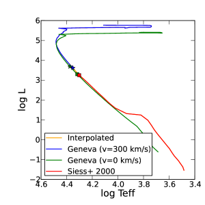
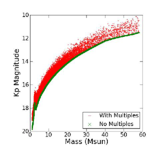
Conversion from stellar masses to synthetic photometry requires the use of stellar evolution and atmosphere models. At the suspected age of the young cluster (4$-$8 Myr), stars with masses in excess of 30-60 M_⊙ are evolving off the main-sequence and stellar evolution models with rotation are found to best describe populations of blue supergiants and Wolf-Rayet stars (Meynet & Maeder, 2003). We use the grid of Geneva models with an initial rotation speed of 300 km/s provided by Meynet & Maeder (2003), which only extends down to 9 M_⊙ . In these models, Wolf-Rayet stars are identified using the criteria suggested in Meynet & Maeder (2003): $T_{eff}>10^{4}$ K and the mass fraction of hydrogen at the surface is $X_{s}<0.4$. To extend to lower masses along the main sequence and also capture pre-main sequence evolution at younger ages, the Geneva grid is merged with the grid of models provided by Siess et al. (2000) that extends up to 7 M_⊙ . For both grids, a suite of isochrones is generated at logarithmic ages of $\log t=6.0-7.4$ with steps of $\Delta\log t=0.01$ and each isochrone samples mass more finely than $\Delta m=0.005$ M_⊙ . The two isochrones are then merged and interpolated over the gap between the two models (7-9 M_⊙ ). An example of the merging process for $\log t=6.8$ is shown in Figure 2. The resulting isochrones provide a mapping from the simulated stellar masses to their luminosities ($L$), effective temperatures ($T_{eff}$) and surface gravities ($g$).

The physical parameters for each star are converted into observable brightness at Kp-band using model stellar atmospheres. Again, there is no single set of atmosphere models that spans the full range of effective temperatures and surface gravities. For hot stars with $T_{eff}>7000$ K, atmosphere models by Castelli & Kurucz (2003) are used for all non-Wolf-Rayet stars. For temperatures of 4000 K $<T_{eff}<$ 7000 K, we use the NextGen models of Hauschildt et al. (1999) and for $T_{eff}<$ 4000 K we use the updated NextGen models with improved AMES opacities (Allard et al., 2000). The grids do not intersect exactly at the transition temperatures; however, synthetic broadband photometry differs by $\lesssim$2% in the K-band, which is less than our photometric precision, so no interpolation between the different atmosphere models is done. All downloaded atmosphere models were re-formatted to work with the pysynphot python package in order to perform interpolations within each grid and generate synthetic spectra at specific temperatures, metallicities, and gravities. The synthetic spectra are flux calibrated to what would be observed at Earth without extinction by multiplying by $(R/d)^{2}$, where $R$ is the radius of the star and $d$ is the distance. Then the synthetic spectra are reddened using the Galactic Center extinction law from Nishiyama et al. (2009) and convolved with transmission profiles for a typical Mauna Kea atmosphere and for the Kp filter in NIRC2. The final synthetic spectra are integrated using pysynphot to produce broad-band Kp photometry as would be seen from the telescope. An example mass-Kp magnitude relation is shown in Figure 5 (left panel) and would predict that S0-2, with a Kp$=14.39$ after correcting to A${}_{Ks}=2.7$, would have a mass of $\sim$18 M_⊙ , which is consistent with previous estimates based on the effective temperature and surface gravity derived from detail spectral analysis (Martins et al., 2008).

Figure 2.— 6 Myr luminosity-effective temperature isochrones from various stellar evolution models used to construct and test a combined grid of stellar evolution models that spans ages from 1-25 Myr and the full range of stellar masses. Geneva models without rotation spanning 0.8$-$120 M_⊙ are shown in green as a baseline (Schaller et al., 1992). The observed post-main-sequence evolution of massive stars at this age is best described with models that include rotation. The isochrone from Geneva models with rotation, shown in blue, differs significantly in luminosity. Models with rotation only extend down to 9 M_⊙ (blue star and green star). Models provided by Siess et al. (2000) are used for main sequence and pre-main sequence models below 7 M_⊙ and are shown in red (7 M_⊙ point also shown as a red square and green square). The blue and red isochrones are merged and interpolated over the gap to construct final isochrones, shown in orange, used in our cluster modeling.

Wolf-Rayet (WR) stars require special consideration as their atmospheres are windy and clumpy. Models of stellar evolution for WR stars can predict when stars enter and exit the WR phase, surface abundances, and the luminosities and temperatures at the base of the atmosphere. However, this is insufficient to uniquely define what will be observed due to differences in wind velocities, mass loss rates, and clumping factors (e.g. Hamann et al., 2008). Put another way, there is no unique mass-magnitude relationship for Wolf-Rayet stars. Model atmospheres do exist for Wolf-Rayet stars; but they require observations of the wind velocities and mass-loss rates and still do not uniquely predict the interior properties of the star, such as temperature and gravity at the base of the atmosphere (Martins et al., 2007). Therefore, the observed magnitudes of the Wolf-Rayet stars cannot be used in a straightforward manner and we exclude them from the analysis of the luminosity function. The number of WR stars, N_WR relative to the number of OB stars is still a powerful constraint on the age and mass of the cluster and we incorporate N_WR into our Bayesian analysis.

Table 1Model Cluster Parameters

Parameter	Vary?	Description	Prior
$\alpha$	free	IMF slope between $m_{min}$ and $m_{max}$	Uniform from [0.10, 3.35]
$\log t$	free	log10( age of the young cluster in years )	Gaussian with $\bar{\log t}=6.78$, $\sigma=0.18$ from [6.20, 6.70]
$M_{cl,obs}$	free	initial mass of the young cluster	Uniform from [103, 105] M⊙
d	free	distance to the young cluster	Gaussian with $\bar{d}=8.096$ kpc, $\sigma=0.483$ kpc from [6.793, 9.510]
$m_{min}$	fixed	IMF minimum stellar mass	1 M⊙
$m_{max}$	fixed	IMF maximum stellar mass	150 M⊙
Z	fixed	metallicity of the young cluster	0.20 (roughly solar)
AKs	fixed	extinction to the young cluster	2.7
MF_amp	fixed	MF function’s amplitude	0.44
MF_index	fixed	MF function’s power-law index	0.51
CSF_amp	fixed	CSF function’s amplitude	0.50
CSF_index	fixed	CSF function’s power-law index	0.45
CSF_max	fixed	maximum value for CSF	3
$\beta$	fixed	power-law index for $q$ distribution	-0.4

3.2. Bayesian Methodology

A Bayesian inference approach is used to determine the physical properties of the YNC at the Galactic center. This methodology is generally applicable to the analysis of other star clusters. The advantages of Bayesian inference for astronomical applications are highlighted in Press (1997) and have been widely adopted in cosmology (Hobson et al., 2010). Bayesian techniques are beginning to be used more widely in the study of all types of star clusters (Selman et al., 1999; Allen et al., 2005; Converse & Stahler, 2008; De Gennaro et al., 2009; van Dyk et al., 2009; Espinoza et al., 2009; Rizzuto et al., 2011). The analysis presented here differs from previous work in several ways. First, single-band photometric information is combined with some spectroscopic information that identify which stars are Wolf-Rayet stars. In our case, only single band photometry is necessary since extinction maps are available from past multi-band photometry (Schödel et al., 2010). Second, the initial mass function is assumed to have the functional form of a truncated power-law, although other functional forms can easily be inserted. This differs from some Bayesian treatments that attempt to derive the masses of the individual stars allowing for infinite variation in the shape of the mass function (Converse & Stahler, 2008; van Dyk et al., 2009; De Gennaro et al., 2009). Third, we allow for mass-dependent multiplicity fractions and high-order multiple systems, which are important at the high mass end of the mass function. Fourth, we include all candidate young stars and weight them by their probability of youth in order to use all available information and accurately account for incompleteness. Finally, instead of using Markov Chain Monte Carlo techniques to perform the Bayesian inference, we find that better solutions result from nested sampling techniques (Feroz & Hobson, 2008; Feroz et al., 2009). This Bayesian approach provides detailed probability distributions for the mass function slope and other cluster parameters given limited observations. It also avoids traditional biases from binning and neglecting photometric errors and accounts for stochastic sampling of stellar masses. Our full methodology is described below in more detail.

We start at the beginning, with Bayes equation

$$p(\Theta|D)=\frac{p(D|\Theta)p(\Theta)}{p(D)}$$ (6)

where $D$ is the observed data, $\Theta$ is the model, $p(D|\Theta)$ is the likelihood of observing the data given some model, $p(\Theta)$ captures the prior knowledge on the model parameters, and $p(D)$ is a normalizing factor known as the evidence. The likelihood function and the prior distributions then give posterior probability distributions for the model parameters, $p(\Theta|D)$. The model, $\Theta$, is defined by the set of free and fixed parameters given in Table 1.

The data, $D$, is constructed from the sample of candidate young stars ($p_{yng}>0$) brighter than Kp$=$15.5 as described in §2. The WR stars are separated out and only the observed number of WR stars, $N_{WR}$, is included in our analysis, since the initial masses of WR stars cannot be determined based on their luminosity alone. For all the other non-WR stars, measurements of the Kp brightness and error are used along with the probability that each star is young, $p_{yng}$. Although we observe $N_{obs}$ non-WR stars, not all of them are young. We estimate the number of young OB stars, $N_{OB}$, as the sum of the observed non-WR stars, weighted by their probability of youth: $N_{OB}=\sum_{i=1}^{N_{obs}}p_{yng,i}$. The resulting measurements that make up the data are then

$$D=[N_{WR},\mathbf{k_{obs}},N_{OB}]$$ (7)

where $\mathbf{k_{obs}}$ is the set of $\{k_{i},\,\sigma_{k_{i}},\,p_{yng,i}\}$ measurements for the $N_{obs}$ non-Wolf Rayet stars observed.

The likelihood function is composed of three independent probabilities: (1) the likelihood of observing the set of Kp magnitudes, $\{k_{i}\}$, and uncertainties, $\{\sigma_{k_{i}}\}$, which effectively captures the shape of the KLF; (2) the likelihood of observing $N_{OB}$ OB stars, which captures the normalization of the KLF; and (3) the likelihood of observing $N_{WR}$ Wolf-Rayet stars:

$$p(D|\Theta)=p(\mathbf{k_{obs}}|\Theta)\cdot p(N_{OB}|\Theta).\cdot p(N_{WR}|\Theta).$$ (8)

To derive the first term, we use an unbinned approach such that the likelihood is the multiplication of the individual stars’ probabilities, weighted by the probability of youth,

$$p(\mathbf{k_{obs}}|\Theta)=\prod_{i=1}^{N_{obs}}p(k_{i}|\Theta)^{p_{yng,i}}.$$ (9)

The probability for a star to have some Kp, $p(k_{i}|\Theta)$, is given by the probability distribution derived from synthetically “observing” a simulated young cluster. First, the cluster is simulated with model parameters describing the age ($t$), IMF slope ($\alpha$), cluster mass ($M_{cl,obs}$), and the cluster distance ($d$),

$$p(k|\Theta)_{intrinsic}=\textrm{Simulated Yng Cluster}(t,\alpha,M_{cl,obs},d).$$ (10)

These free parameters along with their priors are given in Table 1. The resulting Kp photometry from the simulated stars in the model cluster are binned finely (0.1 mag bins) to produce a probability distribution for the intrinsic Kp luminosities. For small numbers of stars, stochastic sampling effects can lead to an inaccurate estimate of the probability distribution. Therefore, in order to maximize accuracy and reduce the total number of clusters that need to be simulated, all model young clusters are simulated with a total mass of $10^{6}$ M_⊙ . The shape of the Kp luminosity function does not change with cluster mass and the number of Wolf-Rayet and non-Wolf-Rayet stars simply scales linearly with total cluster mass. The intrinsic probability distribution for Kp luminosities is multiplied by the imaging completeness curve, $C(k)$, truncated at Kp$=$15.5 to match the data, and normalized to give the final probability distribution,

$$p(k|\Theta)_{observed}=\frac{p(k|\Theta)_{intrinsic}\cdot C(k)}{\int^{15.5}_{0}p(k|\Theta)_{intrinsic}\cdot C(k)\;dk}.$$ (11)

Finally, the measured photometric error is incorporated by modeling the observed magnitude as $k_{i}=k^{\prime}+\epsilon$ where $\epsilon$ is drawn from a normal distribution with zero mean and a standard deviation of $\sigma_{k_{i}}$. The resulting probability of observing $k_{i}$ for a given star is then given by

$$p(k_{i}|\Theta)=\int^{\infty}p(k^{\prime}|\Theta)_{observed}\;\frac{1}{\sqrt{2\pi\sigma_{k_{i}}^{2}}}\;e^{\frac{-(k^{\prime}-k_{i})^{2}}{2\sigma_{k_{i}}^{2}}}dk^{\prime},$$ (12)

which is the convolution of the model KLF and the error probability distribution. The resulting probabilities for each star feed into Equation 9 to calculate the first term of the total likelihood in Equation 8. In the second and third terms of the likelihood, the number of OB and WR stars scales linearly with the mass of the young cluster, which was verified with simulations. Thus the same simulated young clusters used to produce $p(k|\Theta)_{intrinsic}$ also give the expected number of WR and OB stars after scaling linearly with cluster mass,

$$\aleph_{WR}(M_{cl,obs})=\aleph_{WR}(10^{6}M_{\odot})\left(\frac{M_{cl,obs}}{10^{6}M_{\odot}}\right)$$ (13)

$$\aleph_{OB}(M_{cl,obs})=\aleph_{OB}(10^{6}M_{\odot})\left(\frac{M_{cl,obs}}{10^{6}M_{\odot}}\right)$$ (14)

where $\aleph_{WR}$ and $\aleph_{OB}$ are the expectation values (means) for the number of WR and non-WR stars, respectively. The likelihood of observing $N_{WR}$ and $N_{OB}$ are then taken as a Poisson distributions

$$p(N_{WR}|\Theta)=\frac{\aleph_{WR}(\Theta)^{N_{WR}}\;e^{\aleph_{WR}(\Theta)}}{N_{WR}!}$$ (15)

$$p(N_{OB}|\Theta)=\frac{\aleph_{OB}(\Theta)^{N_{OB}}\;e^{\aleph_{OB}(\Theta)}}{N_{OB}!}.$$ (16)

3.3. Sampling Posterior Probability Distributions with Multinest

The resulting posterior probability distribution for the model parameters cannot be calculated analytically. Traditionally, Monte Carlo techniques are used to produce a representative sample of points from the posterior probability distribution. The most commonly used method is the Markov Chain Monte Carlo (MCMC). However, MCMC methods may have difficulty converging or fully mapping probability space when the probability distributions that are being sampled are multi-modal or highly degenerate and curved. An alternative method is nested sampling (Skilling, 2004) such as in the publicly available multi-modal nested sampling code, MultiNest (Feroz & Hobson, 2008; Feroz et al., 2009). This algorithm has been successfully demonstrated in cosmology, galaxy evolution, and gravitational wave problems (e.g. Bridges et al., 2009; Kilbinger et al., 2010; Martinez et al., 2011; Veitch & Vecchio, 2010) and is less computationally expensive and more accurate, in some cases, than MCMC methods. We performed tests on simulated clusters using traditional MCMC techniques using both Metropolis-Hastings and Hit-and-Run step methods (PyMC package) and compared the overall computation time and accuracy with the MultiNest code. MultiNest took 5-10 times less computation time and produced more accurate results in all our simulated clusters (see §3.4 for more details). Therefore, we utilized MultiNest in our analysis of the Young Nuclear Star cluster’s IMF.

MultiNest uses a fixed number of points per iteration to sample parameter space and calculate the Bayesian evidence at each point. In successive iterations, the same number of points are concentrated into smaller and smaller volumes centered around the most probable regions. This process continues until the evidence no longer changes by more than a specified tolerance value. We use 1000 points and an evidence tolerance of 0.3 in order to sample parameter space well and run efficiently. We also enabled multi-modal searches as several simulated clusters could clearly be fit by several distinct sets of model parameters.

3.4. Testing on Simulated Clusters

To test the speed and accuracy of our bayesian methodology and codes, clusters were simulated and synthetically “observed” that had different ages, IMFs, and multiplicity properties. The synthetic “observations” were then fit with the bayesian inference techniques described above and the resulting posterior probability distribution functions were examined to see if they produced results consistent with the input cluster parameters. All clusters were simulated at a distance of 8 kpc, an extinction of $A_{Ks}=2.7$, and with a cluster mass aimed at producing a similar number of OB stars to our observed data set. Photometric errors for simulated cluster stars are randomly drawn from the distribution of empirical errors from the GC observations. Tests were performed to (1) understand degeneracies in fitting a cluster’s age, (2) determine the impact of multiplicity, and (3) explore whether we recover both top-heavy and normal IMF slopes.

3.4.1 Age

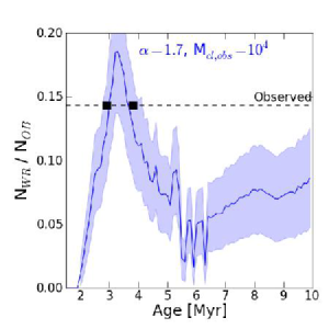
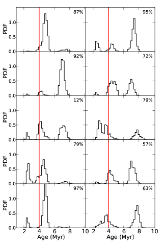
A cluster’s age is often one of the most difficult parameters to constrain, especially at young ages and when only high-mass main-sequence and post-main-sequence stars are observed. The number of WR stars and the ratios of WR to OB stars can be a precise indicator of age; however, there are also cases where degeneracies produce several possible solutions (Paumard et al., 2006). To illustrate these degeneracies we simulate clusters at a range of ages from 1.5 - 10 Myr and examine the ratio of N_WR to N_OB. Note that N_OB includes all OB stars down to Kp$=$15.5, which is equivalent to B1$-$B2 V. Figure 3 shows that N_WR/N_OB initially rises around 2 Myr, peaks at 3 Myr, and falls to a minimum around 6 Myr, which is set almost entirely by the rise and fall of N_WR. After 6 Myr, the ratio rises slightly again as N_WR remains relatively constant, but N_OB begins to drop. If we observe a N_WR/N_OB ratio of 0.125, then there are two possible ages: 2.9 Myr and 3.8 Myr, assuming an IMF slope of $\alpha=1.7$. This degeneracy is not entirely independent of the IMF slope (Figure 3, right panel). In order to explore how our bayesian methodology handles this age degeneracy, we produce ten different realizations of a cluster, all with the same input parameters (t$=$4 Myr, $\alpha=1.7$, M${}_{cl,obs}=10^{4}$ M_⊙ , d$=8$ kpc, single stars). Each cluster is then fit using the Bayesian inference methods described in §3.2. The resulting probability distributions for the age are shown in Figure 4 and multiple age solutions are almost always found. We note that in these 1D marginalized probability distributions, the input cluster age is not always the highest peak. However, the input age is always recovered within the 99% confidence interval and with much higher confidence if each peak is treated as an independent solution in a multi-modal distribution. Given the results of our testing, all further age results will be reported using multi-modal solutions, if necessary.

Figure 3.— Ratio of the number of WR stars to the number of OB stars (Kp$\leq$15.5) as a function of cluster age. This quantity, along with the magnitude of the brightest observed OB stars, provides the strongest constraint on the cluster age; however, it shows degeneracies that often result in multiple solutions for a given cluster. Left: An example cluster with an IMF slope of $\alpha=1.7$ will produce a specific N_WR/N_OB ratio two to three times in the first 10 Myr (blue solid). Right: Changing the IMF slope will shift the ages at which a specific N_WR/N_OB ratio occurs. The observed N_WR/N_OB ratio for the YNC intersects the $\alpha=1.7$ cluster at ages of $\sim$3 and $\sim$4 Myr. Uncertainties due to stochastic sampling (shaded) also suggest that 8-10 Myr may be a plausible solution; but, the presence of bright O giants and supergiants makes these larger ages unlikely.

Figure 4.— Test-clusters’ age posterior probability distributions for 10 different realizations of a cluster with $\alpha=1.7$, t$=$4 Myr, d$=$8 kpc, M${}_{cl,obs}=10^{4}$ M_⊙ , and only single stars. The input age of 4 Myr is marked (vertical red) and the confidence interval that just includes 4 Myr is reported in the top right corner of each panel. The confidence interval is calculated by sorting the probability distribution and integrating starting with the highest bins and proceeding until the bin including 4 Myr is reached. The input age always falls within the 99% confidence interval. If each peak is treated as an independent solution, the input age is recovered with even greater confidence.

3.4.2 Multiplicity

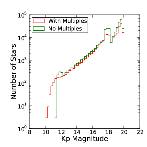
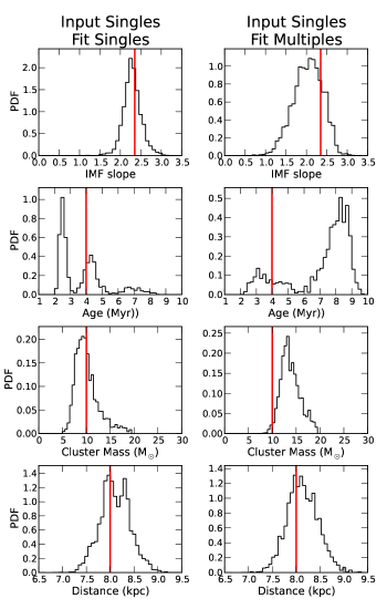
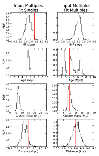
The need to incorporate multiplicity when determining a cluster’s initial mass function is often discussed (Kroupa, 1995; Goodwin & Kroupa, 2005; Weidner et al., 2009) but rarely implemented due to incomplete knowledge of multiplicity fractions, number of companions, companion mass functions, and how these all scale with primary mass (see Appendix A and references therein). The presence of multiple systems influences the bright end of the KLF as illustrated in Figure 5 by populating the brightest magnitude bins (Kp$<$11) with sources that would otherwise be much fainter single stars. We tested two possible scenarios to explore the impact of multiplicity in our analysis. First, a cluster was simulated with only single stars and analysis was done with and without allowing multiple systems in the fit. Second, a cluster was simulated with multiple systems and, again, analysis was done with and without allowing multiple systems in the fit. Both clusters had an IMF slope of $\alpha=2.35$, an age of 4 Myr, and a mass of $10^{4}$ M_⊙ , although similar tests were performed with different IMF slope and age combinations and the results are robust. Figure 6 shows the results for the simulated cluster containing only single stars. Incorrectly fitting this cluster with multiple systems produces extremely biased estimates for the cluster age and only slight biases in the IMF slope and cluster mass. Without prior information, it is difficult to discern that an inaccurate multiplicity model is being used. Figure 7 shows the results for the simulated cluster containing multiple systems. Incorrectly fitting this cluster with single stars produces extremely biased estimates for nearly all the parameters. Even without prior information, it is easy to discern that the single-star model is inaccurate since the distance tends toward unphysical low values. Multiple systems in clusters produce Kp magnitudes that are brighter than is allowed in the model clusters with only single stars at 8 kpc. Thus the only way to produce such bright systems is to move the cluster closer in distance. Shifting the cluster to younger ages is also a possibility; but such young clusters do not give the correct number of WR stars. The largest error is made when using single-star model clusters to fit to clusters with multiple systems. Thus, we choose to fit the observed data with simulated clusters containing multiple systems. All additional tests described below used simulated clusters containing multiple systems and were fit with multiples.

Figure 5.— Comparison between the Kp distribution for model clusters with only single stars (green) and with multiple systems (red). Both clusters have the same basic parameters: $t=$4 Myr, $d=$8 kpc, $A_{Ks}=$2.7, and $M_{cl,y}=10^{6}$ M_⊙ . Left: The mass-magnitude relation for two simulated clusters showing that multiple systems with high mass primaries are typically 1 mag brighter than single stars. Right: The binned Kp luminosity function for both clusters. The cluster with multiple systems extends to higher Kp magnitudes than does the cluster with only single stars. We also note the bump at Kp$\sim$18 is the pre-main-sequence turn-on.

Figure 6.— Test-cluster’s marginalized 1D posterior probability density functions (PDF) for a simulated cluster containing only single stars that is subsequently fit allowing only single stars left or multiple systems right. The input values for the cluster’s IMF slope, age, mass, and distance are shown as a vertical red line in each panel. For a cluster containing only single stars, fitting with multiple systems produces extremely biased estimates for the cluster age and only slight biases in the IMF slope and cluster mass. Without prior information, it is difficult to discern that an inaccurate multiplicity model is being used.

Figure 7.— Test-cluster’s marginalized 1D posterior probability density functions (PDF) for a simulated cluster containing multiple star systems that is subsequently fit allowing only single stars left or multiple systems right. The input values for the cluster’s IMF slope, age, mass, and distance are shown as a red line in each panel. For a cluster containing multiple systems, fitting with single stars produces extremely biased estimates for nearly all the parameters. Without prior information, it is easy to discern that an inaccurate multiplicity model is being used since the distance tends toward unphysically low values. Multiple systems in clusters produce bright systems that are brighter than is allowed in the model clusters with only single stars at 8 kpc. Thus the only way to produce such bright systems is to move the cluster closer in distance.

3.4.3 IMF Slope

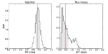
Our bayesian inference methodology shows no systematic biases with respect to the IMF slope as shown in the following tests on synthetic clusters. Two clusters were simulated with an age of 6 Myr and with IMF slopes of $\alpha=2.35$ (Salpeter) and $\alpha=0.45$ (top-heavy reported by Bartko et al. (2010)). The Salpeter-like cluster has an input mass of 10,000 M_⊙ and the top-heavy cluster has an input mass of 40,000 M_⊙ in order to produce $\sim$100 non-WR stars with Kp$\leq$15.5; similar to our observed data set. Figure 8 shows the output posterior probability distributions for the IMF slope, age, and cluster mass for the two simulated clusters. The input IMF slope falls well within the 68% confidence interval of the posterior probability density function. A handful of similar cluster tests were performed with different ages and masses and the input and output IMF slopes always agree within the 68% confidence region and there appears to be no significant bias to either higher or lower IMF slopes.

Figure 8.— Test-cluster’s marginalized 1D posterior probability density functions (PDF) for a simulated cluster with IMF slope = 2.35 (left) and IMF slope = 0.45 (right). The input values for the cluster’s IMF slope, age, mass, and distance are shown as a vertical red lines in each panel. The grey shaded regions represent the 68% confidence interval for the output probability distributions and all of the input values fall within this interval. The confidence intervals are calculated by first finding the peak in the probability distribution and then stepping away from the peak until the integrated probability reaches 68%.

4. Results

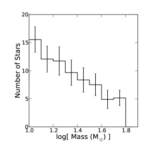
The observed Kp magnitudes, their uncertainties, and the number of Wolf-Rayet and OB stars were used in Bayesian inference to determine the cluster’s physical properties. Figure 9 shows the resulting 1D posterior probability distributions for the 4 free parameters in the model (cluster age, mass, distance, and IMF slope). The model assumes that multiple systems are present with the properties described in §3.1 and Appendix A. Several parameters show correlations including a moderate correlation between the cluster age and IMF slope (Figure 10). The correlation between the cluster mass and the age or IMF slope is a consequence of the age-IMF slope relationship since, at older ages, the most massive stars have dissapeared and the cluster mass must increase to match the observed numbers of stars brighter than Kp$=15.5$. The posterior probability distributions are the most accurate representation of the results; however, we also present “best-fit” values in Table 2 represented by the expectation value and 68% and 95% Bayesian confidence intervals of the marginalized 1D posterior probability density functions. The resulting age distribution is multi-modal. Therefore, we report solutions from three possible samples: (1) ages greater than 3.3 Myr, (2) ages less than or equal to 3.3 Myr, and (3) the complete posteriors, The age boundaries for the two modal solutions were estimated based on the minima between the two peaks. We report all parameters for these three solutions; however, all solutions have similar $\alpha$, M_cl,obs, and $d$ distributions. We will adopt Solution 1 in the remainder of the paper as it contains the most probable solution (with the maximum likelihood) and contains the bulk of the probability density. Solution 1 is also favored over the smaller age in Solution 2 based on more detailed spectroscopic analyses that show the Wolf-Rayet star sub-types and the supergiant nature of the brightest OB stars favor ages $\gtrsim$4 Myr (Paumard et al., 2006; Martins et al., 2007). A comparison of the observed and model KLFs and mass functions from the inferred parameters of Solution 1 is shown in Figure 11. The complete posteriors for the number of predicted Wolf-Rayet and OB stars are also shown in Figure 12 and are compared with the observed number of WR and OB stars. The overall fit is good given the theoretical uncertainty in the evolution of massive stars and the unknown mapping between progenitor mass and Wolf-Rayet phases.

Figure 9.— Observed YNC’s marginalized 1D posterior probability density functions (PDF) for the cluster properties. The histograms show results from the Multinest bayesian analysis including multiple systems. The dashed black lines show the prior probability distributions used. The resulting constraints on the IMF slope (panel a), the cluster age (panel b) and the cluster mass (panel c) are significant compared with the prior PDFs used. The distance constraint (panel d) is weak and is largely a reflection of the prior.

Table 2Cluster Properties and Uncertainties

Cluster	Expectation	68%	95%
Properties	Value	Interval	Interval
Solution 1: Age$>$3.3 Myr
Age (Myr)	4.2	3.6 - 4.8	3.4 - 6.1
IMF slope ($\alpha$)	1.7	1.5 - 1.9	1.1 - 2.1
Integrated Mass ($10^{3}$ M⊙ )	10.1	8.1 - 11.6	7.2 - 18.5
Distance (kpc)	7.9	7.6 - 8.3	7.3 - 8.6
Solution 2: Age$\leq$3.3 Myr
Age (Myr)	2.8	2.6 - 3.1	2.4 - 3.3
IMF slope ($\alpha$)	1.8	1.6 - 1.9	1.5 - 2.1
Integrated Mass ($10^{3}$ M⊙ )	8.8	7.7 - 9.5	6.8 - 10.5
Distance (kpc)	7.9	7.6 - 8.2	7.3 - 8.5
Total
Age	3.6	2.8 - 4.3	2.5 - 5.8
IMF slope ($\alpha$)	1.7	1.5 - 1.9	1.2 - 2.1
Integrated Mass ($10^{3}$ M⊙ )	9.5	7.9 - 10.6	7.1 - 16.7
Distance (kpc)	7.9	7.6 - 8.3	7.3 - 8.6

Note. — The integrated masses correspond to that within the field of view of the survey (see Paper I for details) between 1$-$150 M_⊙ . The estimated mass for the entire YNC is 2-4 times larger.

Figure 10.— 2D posterior probability density functions (PDF) for the observed cluster’s properties. The over-plotted contours give 68%, 95%, and 99% confidence intervals. Weak correlations exist between age, mass, and IMF slope. The correlation between the cluster mass and the age or IMF slope is a consequence of the age-IMF slope relationship since, at older ages, the most massive stars have dissapeared and the cluster mass must increase to match the observed numbers of stars brighter than Kp$=15.5$.

Figure 11.— The observed (black) and model (red) Kp-band luminosity function (left) and the resulting mass function (right). The model cluster includes multiple systems and has the properties listed in Table 2 (Solution 1). (Left): The observed KLF (black line) and number of WR stars (black circle) show good agreement with the model KLF (red line) and model WR stars (red square). The observed Kp magnitudes (red) are corrected for differential extinction to a common extinction value of A${}_{Ks}=2.7$. The model KLF is taken as the mean and standard deviation (red errorbars) of 100 simulated clusters, all with the same parameters, in order to account for variations due to stochastic sampling of the IMF. The imaging completeness curve is applied to each simulated cluster for direct comparison to the observed KLF. (Right): The resulting mass function is constructed by converting the observed stars’ Kp magnitudes to masses using the best-fit isochrone. To capture uncertainties in the stars’ brightness, each star’s Kp magnitude is randomly sampled 100 times from a Gaussian distribution centered on the measured Kp with a width of $\sigma_{Kp}$. The resulting masses are binned into a mass function and the mean and standard deviation of the 100 mass functions are shown as a black line with errorbars. The Wolf-Rayet stars are not included in the mass function.

Figure 12.— Comparison of the observed vs. inferred distributions for the number of Wolf-Rayet stars (left) and the number of OB stars (right). The observed $N_{WR}$ and $N_{OB}$ are shown as vertical black lines and the probability distributions from the Bayesian analysis are shown as histograms.

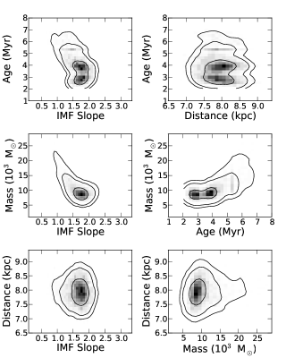
For the IMF slope, recall that a flat prior from 0.5$-$3.5 was adopted; but the posterior distribution is strongly peaked at 1.7 $\pm$ 0.2. The slope is flatter than a typical Salpeter slope and slopes of 2.35 or greater are ruled out at 3.8$\sigma$ (99.98%). The slope is inconsistent with the previously reported top-heavy slope of 0.45 (Bartko et al., 2010) at the 3.8$\sigma$ level (99.98%). Our sample of young stars includes those within r$<$0$\farcs$8; however, the results are very similar even when these stars are excluded (Figure 13, as is done in Bartko et al. (2010).

Figure 13.— Same as Figure 9, but excluding stars with r$<$0$\farcs$8 to better match the sample chosen in (Bartko et al., 2010). The peak of the probability distribution for the IMF slope shifts to $\alpha=$1.6; however, it is consistent with the result from the complete sample, within the 68% uncertainties. IMF slopes as top-heavy as $\alpha=0.45$ remain inconsistent at 99.89% probability. Ages of 6-7 Myr become slightly more probable.

The cluster mass is 10,100 M_⊙ (68% interval: 8,100$-$11,600 M_⊙ ) between 1$-$150 M_⊙ and is well constrained by the data, given that the posterior distribution is significantly different from the prior. The cluster age is also significantly different from the prior and shows multiple peaks. The most probable solution falls at 3.9 Myr (68% interval: 3.6$-$4.8 Myr); although the second peak at 2.8 Myr is still highly probable. This multi-modal behavior is a result of the rapid changes in the number of WR stars and the ratio of WR to OB stars in very short periods of time (Figure 3). Although the distance is also a free parameter, the resulting probability distribution mainly reflects the prior shown in the dashed line. This is reassuring since, in our testing, incorrect model assumptions (e.g. fitting single star models to data with multiple systems) often led to skewed distance distributions, which we do not observe using the multiple systems model.

The cluster mass and the numbers of WR and OB stars are based only on the young stellar population within the field of view observed for this study, which has incomplete azimuthal coverage. This does not represent the entire cluster mass of the young nuclear star cluster. The total cluster mass can be estimated by extrapolating beyond the field of view in this study, in several different ways. First, we use the assumption that the cluster is spherically symmetric and has a surface density profile that falls as $R^{-\Gamma}$ with $\Gamma=0.9$ (Paper I). This yields a surface density weighted coverage of 27% and a coverage-corrected total cluster mass of $\sim$37,000 M_⊙ within a projected radius of 13$\farcs$65 and above 1 M_⊙ . The above assumption fails to account for known kinematic structures in the young population, including a highly inclined disk containing as much as 50% of the young stars. Furthermore, the above mass estimate assumes a constant IMF at all radii, which is unlikely given the mass segregation that will occur over 4 Myr. As an alternative, we instead make an empirically based estimate of the completeness by taking the ratio of the number of young stars with Kp $<$ 13 within our FOV to the same number reported in Paumard et al. (2006), which we assume is 100% complete out to 14”. This yields a coverage completeness of 71% and a total cluster mass of $\sim$14,000 M_⊙ above 1 M_⊙ . Thus, we estimate the total cluster mass to be in the range of 14,000 - 37,000 M_⊙ above 1 M_⊙ . We note that the total cluster mass depends on the low-mass cutoff as M${}_{cl}\cdot$ (m_lo / 1 M_⊙ )^-1.7; and, while we have assumed 1 M_⊙ , the lowest-mass young stars we observe are $\sim$8 M_⊙ . In order to improve the constraints on the total cluster mass, more sensitive and azimuthally complete spectroscopic surveys at large radii are necessary.

The above results are derived from modeling clusters with multiple systems; however, for completeness, we also show the resulting posterior probability distributions for a single-star model in Figure 14. It is clear that the fit is poor. The bias to very small distances indicates that the brightest OB stars combined with the number of WR stars cannot be accurately fit with a single star model. Our modeling indicates that multiple star systems are necessary to fit the observed stellar population. However, we caution that the multiplicity properties were fixed to solar neighborhood values that may not be applicable to the Young Nuclear Cluster. Both the star formation process and subsequent dynamical processing may impact multiplicity.

Figure 14.— Same as Figure 9, but only allowing single stars in the model. The overall fit of the single-star model is poor and produces a strong bias away from the measured distance of 8 kpc. Furthermore, the resulting evidence for this model is substantially lower than for the model that includes multiples.

5. Discussion

The young nuclear star cluster at the Galactic center, at least along the plane of the well-defined clockwise disk, has an IMF slope in the range $\alpha=1.5-1.9$ (68% confidence interval) for stellar masses above $\sim$10 M_⊙ . This is significantly flatter than clusters in the Milky Way disk and field ($\alpha=2.35$). Our measured IMF is in good agreement with X-ray observations showing that X-ray emission from pre-main-sequence stars is reduced by a factor of 10 compared with what is expected from observations of the Orion Nebular Cluster, scaled to the age and distance of the Galactic center (Nayakshin & Sunyaev, 2005). Extrapolating our measured IMF slope down to lower masses produces a factor of 4$-$15 fewer X-ray emitting stars ($0.5-3.0$ M_⊙ ) than would be expected for a slope of $\alpha=2.35$.

An extremely top-heavy IMF is inconsistent with our observations at high significance, in contradiction to previous observations (Bartko et al., 2010). An extensive discussion of the possible observational and analysis differences between our work and previous work is presented in Paper I. Here we reiterate a few key differences. The Bartko et al. (2010) field of view extends predominantly North, out of the plane of the well-defined clockwise disk of young stars. They also remove all young stars in the central 0$\farcs$8 and outside 12”. In the work presented here, the spectroscopic window in which young stars are identified extends from the center to the ESE along the well defined clockwise disk structure. And the entire population of young stars, including those within 0$\farcs$8 of the SMBH, is included in the analysis. We assume that all the young stars were formed in a single star formation event with the same physical conditions giving rise to a constant IMF for all the kinematic sub-groups. As discussed in Sections 1 and 2, the stars in this innermost region were dynamically injected and it still appears to be theoretically possible that they originated from the most recent starburst that produced the young nuclear cluster. Furthermore, restricting our sample of young stars to a radius range of 0$\farcs$8$-$12” does not significantly change the KLF shape. Repeating our Bayesian analysis on this restricted sample produces a similar posterior probability distribution for the IMF slopes to that of our full sample.

We find a cluster that is well fit with an instantaneous star formation event at an age of 2.5-5.8 Myr with 95% confidence. The most probable age is 3.9 Myr. This is smaller than the 6 Myr commonly adopted, although consistent within the uncertainty range reported in Paumard et al. (2006). The age of the cluster is mainly constrained by the number of WR stars and the highest luminosity OB stars detected, since this effectively gives a main-sequence turn-off age. Careful examination of Figure 11 in Paumard et al. (2006) shows that best-fit ages, given the different numbers of O and WR stars (WN, WC, WNE, WNL), are actually either 4 Myr or 8 Myr, with 6 Myr being improbable for a Salpeter IMF. The inclusion of fainter OB stars in our spectroscopic sample substantially reduces the probability of cluster ages as old as 8 Myr. Figure 3 shows the expected number of WR and OB stars and their ratio as a function of cluster age for different assumed mass functions. While our Bayesian analysis captures uncertainties in the age due to random sampling of the mass function, it does not capture systematic uncertainties in models of stellar evolution. The lifetimes and luminosities of WR stars are sensitive to metallicity (Fe and $\alpha$ elements), mass-loss rates, initial rotation rates, and close-binary mass exchange. Increased metallicity, mass-loss rates, rotation rates, and binary mass exchange all tend to increase the ages at which WR stars still exist (Eldridge & Vink, 2006; Meynet et al., 2006). On the other hand, increased metallicity reduces the main-sequence lifetimes. Furthermore, massive clusters, such as Westerlund 1, contain WR stars, blue supergiants, yellow hypergiants, and red supergiants at an age of 5 Myr; which no stellar evolution model successfully predicts (e.g. Negueruela et al., 2010). Therefore, we caution that ages up to 8 Myr may still be reasonable given current uncertainties in massive-star evolutionary models. We note that the IMF slope measurement is dominated by the relative luminosity distribution of OB main-sequence and supergaint stars, rather than the numbers of windy WR stars, and is far less sensitive to systematic uncertainties in evolutionary models. If the young nuclear cluster does have a slightly younger age of $\sim$4 Myr, then there are important implications for the dynamical history of the cluster. For instance, models of in situ star formation with a circular gas disk as the initial condition require at least 6 Myr for the orbital eccentricities to evolve from circular to the observed eccentricity distribution peaked at $e=0.3$, assuming a Salpeter IMF (Alexander et al., 2007; Cuadra et al., 2008). Revised calculations are necessary to determine whether the observed IMF slope and younger age can give rise to the observed high eccentricities in such a short time.

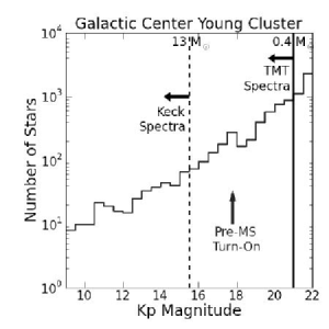
Ultimately, a complete spectroscopic and astrometric census of the young population in the Young Nuclear Cluster is required to accurately measure the recent star formation history and determine if the distinct kinematic components were formed under different conditions, resulting in different mass functions. Expanding the survey area with current facilities will help clarify whether young stars on and off the disk have a different IMF. The Bayesian methodology presented here should be expanded to incorporate additional information from spectroscopy, such as effective temperature and gravity constraints for the OB stars, surface-abundance sub-types for the Wolf-Rayet stars, and luminosities/temperatures from Wolf-Rayet wind/atmosphere modeling such as presented in Martins et al. (2007). This additional information may improve age constraints; although uncertainties in stellar evolution for massive stars will still be a major factor. In the future, detection of pre-main-sequence turn-on points at Kp=17.5 would more definitively constrain the age and star formation history. Furthermore, to truly constrain physical models of star formation at the Galactic center relative to local star formation processes, we will need measurements of the IMF shape over a broader mass range, ideally including any turnover suggesting a characteristic mass scale (e.g. $\sim$0.5 M_⊙ in Orion). Some theories of star formation suggest that in extreme conditions, such as those found at the Galactic center, the characteristic mass may be significantly higher than in local star-forming regions (Morris, 1993; Bonnell et al., 2004; Krumholz & McKee, 2008). Measurements of both the characteristic mass and the pre-main-sequence turn-on point should be possible with the next generation of large ground-based telescopes equipped with adaptive optics-fed integral field spectrographs. One such instrument is IRIS on the Thirty Meter Telescope (TMT), which can accurately spectral-type stars in the Galactic center down to Kp$=$21 in 1 hour (Wright et al., 2010), as shown in Figure 15. Predicted IRIS sensitivities reach 0.4 M_⊙ stars (Kp$=$21); however, distinguishing the young low-mass objects from the sea of much older main-sequence stars may require substantially higher signal-to-noise to make precise measurements of effective temperatures. Such observations will be essential as the Young Nuclear Cluster is one of the few environments where significant deviations have been found from an otherwise near-universal IMF.

Figure 15.— A model Kp-band luminosity function for the Young Nuclear Cluster showing the relative sensitivity of Keck spectroscopy (Kp$<$15.5) and future TMT+IRIS spectroscopy (Kp$<$21). With TMT+IRIS, the pre-main-sequence turn-on point will be detectable at Kp$\sim$17.5 as well as the full IMF shape down to $\sim$0.4 M_⊙ . The model cluster shown here has an IMF slope of 1.7 down to 0.5 M_⊙ and then turns over at 0.5 M_⊙ to a slope of 1.3 down to 0.1 M_⊙ as suggested by Weidner & Kroupa (2004) for star formation in the local neighborhood. The model cluster has a distance of 8 kpc and an extinction of A${}_{Ks}=2.7$.

6. Conclusions

The Galactic center hosts a young nuclear star cluster around the supermassive black hole. We use membership probabilities derived from spectroscopy, precise infrared photometry, and Bayesian inference methods to determine the global properties of the cluster. The best-fit age of the cluster is 3.9 Myr, somewhat younger than previously reported. The cluster’s total mass extrapolated down to 1 M_⊙ is between 14,000 - 37,000 M_⊙ after correcting for incomplete azimuthal coverage. The best-fit IMF slope of 1.7 is flatter than a traditional Salpeter IMF; but far steeper than previously claimed in the literature. Future spectroscopic observations covering a larger field of view and extending to lower masses are necessary to understand the impact of mass segregation on IMF slope measurements and to determine whether the peak in the initial mass function also shows any significant difference from nearby star-forming regions.

Appendix A Multiplicity

The distribution of multiple star systems can be described completely by equations for the multiplicity frequency (MF), the companion star frequency (CSF), the mass ratio (q), and the separation distribution. For star clusters at the distance of the Galactic center (8 kpc), multiple systems are spatially unresolved and the separation distribution can be integrated over. The multiplicity frequency and companion star frequency are defined as in Reipurth & Zinnecker (1993)

$$MF=\frac{B+T+Q+…}{S+B+T+Q+...}$$ (A1)

$$CSF=\frac{B+2T+3Q+…}{S+B+T+Q+...}$$ (A2)

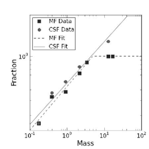
where S is the number of single stars, B is the number of binaries, T is the number of triples, and Q is the number of quadruples. The multiplicity fraction always ranges between 0 and 1; but the companion star fraction, which is the mean number of companions, can be greater than 1, such as for the Orion Trapezium stars where CSF$>$1.5 (Preibisch et al., 1999; Zinnecker & Yorke, 2007). Based on observations, the MF and CSF are known to vary with primary star mass, the age of a cluster, and possibly the density of a cluster (e.g. Ghez et al., 1993; Petr et al., 1998; Mason et al., 1998; Duchêne et al., 1999; Köhler et al., 2000; Reipurth, 2000; Patience et al., 2002; Shatsky & Tokovinin, 2002; Köhler et al., 2006; Duchêne et al., 2007; Köhler et al., 2008; Mason et al., 2009; Raghavan et al., 2010; Kraus & Hillenbrand, 2012). Complete multiplicity surveys of young clusters ($<$10 Myr) that span a large range of primary stellar masses (0.1 $-$ $>10$ M_⊙ ), mass ratios, and separations are difficult to conduct and only a few exist in the literature (Lafrenière et al., 2008; Kobulnicky & Fryer, 2007; Kouwenhoven et al., 2007). Star formation theories do not yet predict an analytic functional form for the MF, CSF, and q distributions and how they vary with primary mass; however, simulations are beginning to produce distributions that are in rough agreement with observations (Bate, 2012; Krumholz et al., 2012). Therefore, we take an empirical approach and compile measurements of the MF and CSF as a function of mass from published surveys of young clusters ($<$10 Myr), which span stellar masses of 0.2$-$17 M_⊙ and all separations (Table 3). This compilation is incomplete as we exclude surveys that only report multiplicity for masses below 1 M_⊙ and those without CSF information. The above high-mass limit is set by the available multiplicity surveys. and the low-mass cutoff is chosen as a reasonable detection threshold for stars in more distant massive young clusters with both current (e.g. Keck) and future (e.g. TMT) spectroscopy. The compiled MF and CSF data (Figure 16) are fit with a power-law dependence on mass and give the following results:

$$MF(m)=Am^{\gamma}\;\;\;\;\;\;A=0.44\;\;\;\gamma=0.51$$ (A3)

$$CSF(m)=Bm^{\beta}\;\;\;\;\;\;B=0.50\;\;\;\beta=0.45$$ (A4)

The best-fit power laws are also shown in Figure 16. For any star cluster older than a few crossing times, the CSF will not continue to grow indefinitely at high masses due to the dynamical instability of high-order systems in a clustered environment. A hard limit to the mean number of companions is adopted (CSF$\leq$3) such that systems with more than 3 components are allowed, but have a low probability of occurrence. Lastly, some observations suggest multiplicity properties may evolve over time differently for clusters with different masses or stellar densities (e. g. Kroupa, 1995; Duchêne et al., 1999; Köhler et al., 2006; Marks & Kroupa, 2012). However, the completeness and significance of these results is still uncertain (King et al., 2012) and we therefore assume all young clusters ($<$10 Myr) have the same multiplicity properties, including the Young Nuclear Cluster.

Table 3Multiplicity Measurements for Young Clusters

Mass (M⊙ )	MF	CSF	Reference
0.175	0.16	0.16	Cha I, Lafrenière et al. (2008)
0.390	0.33	0.37	Cha I, Lafrenière et al. (2008)
0.915	0.38	0.50	Cha I, Lafrenière et al. (2008)
2.14	0.63	0.75	Cha I, Lafrenière et al. (2008)
3.4	0.85	-	Sco OB2, Kouwenhoven et al. (2007)
12.7	1.00	1.5	Orion (ONC), Preibisch et al. (1999)
16.8	1.00	-	Cyg OB2, Kobulnicky & Fryer (2007)

Figure 16.— The multiplicity frequency (MF) and the companion star frequency (CSF) as a function of primary mass. Empirical measurements are plotted for the MF (blue squares) and CSF (red circles) values reported in the literature (Table 3). The data are fit with power laws (lines) as given by Equations A3 and A4. The CSF is truncated at $\leq$3, which impacts systems with a primary mass above $\sim$40 M_⊙ .

Facilities: Keck: II (NIRC2), Keck: II (OSIRIS)

References

- Alexander et al. (2008) Alexander, R. D., Armitage, P. J., Cuadra, J., & Begelman, M. C. 2008, ApJ, 674, 927
- Alexander et al. (2007) Alexander, R. D., Begelman, M. C., & Armitage, P. J. 2007, ApJ, 654, 907
- Allard et al. (2000) Allard, F., Hauschildt, P. H., & Schwenke, D. 2000, ApJ, 540, 1005
- Allen et al. (1990) Allen, D. A., Hyland, A. R., & Hillier, D. J. 1990, MNRAS, 244, 706
- Allen et al. (2005) Allen, P. R., Koerner, D. W., Reid, I. N., & Trilling, D. E. 2005, ApJ, 625, 385
- Bartko et al. (2009) Bartko, H., et al. 2009, ApJ, 697, 1741
- Bartko et al. (2010) Bartko, H., et al. 2010, ApJ, 708, 834
- Baruteau et al. (2011) Baruteau, C., Cuadra, J., & Lin, D. N. C. 2011, ApJ, 726, 28
- Bate (2012) Bate, M. R. 2012, MNRAS, 419, 3115
- Bender et al. (2005) Bender, R., et al. 2005, ApJ, 631, 280
- Blum et al. (1995) Blum, R. D., Depoy, D. L., & Sellgren, K. 1995, ApJ, 441, 603
- Bonnell et al. (2004) Bonnell, I. A., Vine, S. G., & Bate, M. R. 2004, MNRAS, 349, 735
- Bridges et al. (2009) Bridges, M., Feroz, F., Hobson, M. P., & Lasenby, A. N. 2009, MNRAS, 400, 1075
- Brown et al. (2007) Brown, W. R., Geller, M. J., Kenyon, S. J., Kurtz, M. J., & Bromley, B. C. 2007, ApJ, 671, 1708
- Carr et al. (2000) Carr, J. S., Sellgren, K., & Balachandran, S. C. 2000, ApJ, 530, 307
- Castelli & Kurucz (2003) Castelli, F., & Kurucz, R. L. 2003, in IAU Symposium, Vol. 210, Modelling of Stellar Atmospheres, ed. N. Piskunov, W. W. Weiss, & D. F. Gray, 20P
- Converse & Stahler (2008) Converse, J. M., & Stahler, S. W. 2008, ApJ, 678, 431
- Cuadra et al. (2008) Cuadra, J., Armitage, P. J., & Alexander, R. D. 2008, MNRAS, 388, L64
- Cunha et al. (2007) Cunha, K., Sellgren, K., Smith, V. V., et al. 2007, ApJ, 669, 1011
- De Gennaro et al. (2009) De Gennaro, S., von Hippel, T., Jefferys, W. H., et al. 2009, ApJ, 696, 12
- Do et al. (2012) Do, T., Lu, J. R., Ghez, A. M., et al. 2012, submitted to ApJ
- Duchêne et al. (2007) Duchêne, G., Bontemps, S., Bouvier, J., et al. 2007, A&A, 476, 229
- Duchêne et al. (1999) Duchêne, G., Bouvier, J., & Simon, T. 1999, A&A, 343, 831
- Eckart & Genzel (1997) Eckart, A., & Genzel, R. 1997, MNRAS, 284, 576
- Eisenhauer et al. (2005) Eisenhauer, F., et al. 2005, ApJ, 628, 246
- Ekström et al. (2012) Ekström, S., et al. 2012, A&Ain press
- Eldridge & Vink (2006) Eldridge, J. J., & Vink, J. S. 2006, A&A, 452, 295
- Espinoza et al. (2009) Espinoza, P., Selman, F. J., & Melnick, J. 2009, A&A, 501, 563
- Feroz & Hobson (2008) Feroz, F., & Hobson, M. P. 2008, MNRAS, 384, 449
- Feroz et al. (2009) Feroz, F., Hobson, M. P., & Bridges, M. 2009, MNRAS, 398, 1601
- Genzel et al. (2000) Genzel, R., Pichon, C., Eckart, A., Gerhard, O. E., & Ott, T. 2000, MNRAS, 317, 348
- Genzel et al. (2003) Genzel, R., et al. 2003, ApJ, 594, 812
- Gerhard (2001) Gerhard, O. 2001, ApJ, 546, L39
- Ghez et al. (1998) Ghez, A. M., Klein, B. L., Morris, M., & Becklin, E. E. 1998, ApJ, 509, 678
- Ghez et al. (2000) Ghez, A. M., Morris, M., Becklin, E. E., Tanner, A., & Kremenek, T. 2000, Nature, 407, 349
- Ghez et al. (1993) Ghez, A. M., Neugebauer, G., & Matthews, K. 1993, AJ, 106, 2005
- Ghez et al. (2005) Ghez, A. M., Salim, S., Hornstein, S. D., et al. 2005, ApJ, 620, 744
- Ghez et al. (2003) Ghez, A. M., et al. 2003, ApJ, 586, L127
- Ghez et al. (2008) Ghez, A. M., et al. 2008, ApJ, 689, 1044
- Gillessen et al. (2009a) Gillessen, S., Eisenhauer, F., Fritz, T. K., et al. 2009a, ApJ, 707, L114
- Gillessen et al. (2009b) Gillessen, S., Eisenhauer, F., Trippe, S., et al. 2009b, ApJ, 692, 1075
- Goodman (2003) Goodman, J. 2003, MNRAS, 339, 937
- Goodwin & Kroupa (2005) Goodwin, S. P., & Kroupa, P. 2005, A&A, 439, 565
- Gürkan & Rasio (2005) Gürkan, M. A., & Rasio, F. A. 2005, ApJ, 628, 236
- Haas et al. (2011) Haas, J., Šubr, L., & Kroupa, P. 2011, MNRAS, 412, 1905
- Haas (2010) Haas, M. R. 2010, PhD thesis, Ph. D. thesis, University of Leiden (2010)
- Hamann et al. (2008) Hamann, W.-R., Gräfener, G., Feldmeier, A., et al. 2008, in Astronomical Society of the Pacific Conference Series, Vol. 391, Hydrogen-Deficient Stars, ed. A. Werner & T. Rauch, 293
- Hansen & Milosavljević (2003) Hansen, B. M. S., & Milosavljević, M. 2003, ApJ, 593, L77
- Hauschildt et al. (1999) Hauschildt, P. H., Allard, F., & Baron, E. 1999, ApJ, 512, 377
- Hobbs & Nayakshin (2009) Hobbs, A., & Nayakshin, S. 2009, MNRAS, 394, 191
- Hobson et al. (2010) Hobson, M. P., Jaffe, A. H., Liddle, A. R., Mukeherjee, P., & Parkinson, D. 2010, Bayesian Methods in Cosmology, ed. Hobson, M. P., Jaffe, A. H., Liddle, A. R., Mukeherjee, P., & Parkinson, D.
- Kilbinger et al. (2010) Kilbinger, M., et al. 2010, MNRAS, 405, 2381
- Kim et al. (2004) Kim, S. S., Figer, D. F., & Morris, M. 2004, ApJ, 607, L123
- Kim & Morris (2003) Kim, S. S., & Morris, M. 2003, ApJ, 597, 312
- Kiminki & Kobulnicky (2012) Kiminki, D. C., & Kobulnicky, H. A. 2012, ApJ, 751, 4
- Kiminki et al. (2007) Kiminki, D. C., et al. 2007, ApJ, 664, 1102
- King et al. (2012) King, R. R., Parker, R. J., Patience, J., & Goodwin, S. P. 2012, MNRAS, 421, 2025
- Kobulnicky & Fryer (2007) Kobulnicky, H. A., & Fryer, C. L. 2007, ApJ, 670, 747
- Köhler et al. (2000) Köhler, R., Kunkel, M., Leinert, C., & Zinnecker, H. 2000, A&A, 356, 541
- Köhler et al. (2008) Köhler, R., Neuhäuser, R., Krämer, S., et al. 2008, A&A, 488, 997
- Köhler et al. (2006) Köhler, R., Petr-Gotzens, M. G., McCaughrean, M. J., et al. 2006, A&A, 458, 461
- Kolykhalov & Syunyaev (1980) Kolykhalov, P. I., & Syunyaev, R. A. 1980, Soviet Astronomy Letters, 6, 357
- Kouwenhoven et al. (2009) Kouwenhoven, M. B. N., Brown, A. G. A., Goodwin, S. P., Portegies Zwart, S. F., & Kaper, L. 2009, A&A, 493, 979
- Kouwenhoven et al. (2007) Kouwenhoven, M. B. N., Brown, A. G. A., Portegies Zwart, S. F., & Kaper, L. 2007, A&A, 474, 77
- Krabbe et al. (1991) Krabbe, A., Genzel, R., Drapatz, S., & Rotaciuc, V. 1991, ApJ, 382, L19
- Krabbe et al. (1995) Krabbe, A., et al. 1995, ApJ, 447, L95
- Kraus & Hillenbrand (2012) Kraus, A. L., & Hillenbrand, L. A. 2012, ApJ, 757, 141
- Kroupa (1995) Kroupa, P. 1995, MNRAS, 277, 1491
- Krumholz et al. (2012) Krumholz, M. R., Klein, R. I., & McKee, C. F. 2012, ApJ, 754, 71
- Krumholz & McKee (2008) Krumholz, M. R., & McKee, C. F. 2008, Nature, 451, 1082
- Lafrenière et al. (2008) Lafrenière, D., Jayawardhana, R., Brandeker, A., Ahmic, M., & van Kerkwijk, M. H. 2008, ApJ, 683, 844
- Lauer et al. (1998) Lauer, T. R., Faber, S. M., Ajhar, E. A., Grillmair, C. J., & Scowen, P. A. 1998, AJ, 116, 2263
- Levin & Beloborodov (2003) Levin, Y., & Beloborodov, A. M. 2003, ApJ, 590, L33
- Löckmann et al. (2009) Löckmann, U., Baumgardt, H., & Kroupa, P. 2009, MNRAS, 398, 429
- Lu et al. (2005) Lu, J. R., Ghez, A. M., Hornstein, S. D., Morris, M., & Becklin, E. E. 2005, ApJ, 625, L51
- Lu et al. (2009) Lu, J. R., Ghez, A. M., Hornstein, S. D., et al. 2009, ApJ, 690, 1463
- Madigan et al. (2011) Madigan, A.-M., Hopman, C., & Levin, Y. 2011, ApJ, 738, 99
- Maillard et al. (2004) Maillard, J. P., Paumard, T., Stolovy, S. R., & Rigaut, F. 2004, A&A, 423, 155
- Maíz Apellániz (2008) Maíz Apellániz, J. 2008, ApJ, 677, 1278
- Maíz-Apellániz (2009) Maíz-Apellániz, J. 2009, Ap&SS, 324, 95
- Maíz Apellániz & Úbeda (2005) Maíz Apellániz, J., & Úbeda, L. 2005, ApJ, 629, 873
- Marks & Kroupa (2012) Marks, M., & Kroupa, P. 2012, A&A, 543, A8
- Martinez et al. (2011) Martinez, G. D., Minor, Q. E., Bullock, J., et al. 2011, ApJ, 738, 55
- Martins et al. (2007) Martins, F., Genzel, R., Hillier, D. J., et al. 2007, A&A, 468, 233
- Martins et al. (2008) Martins, F., Gillessen, S., Eisenhauer, F., et al. 2008, ApJ, 672, L119
- Mason et al. (2009) Mason, B. D., Hartkopf, W. I., Gies, D. R., Henry, T. J., & Helsel, J. W. 2009, AJ, 137, 3358
- Mason et al. (1998) Mason, B. D., Henry, T. J., Hartkopf, W. I., ten Brummelaar, T., & Soderblom, D. R. 1998, AJ, 116, 2975
- McMillan & Portegies Zwart (2003) McMillan, S. L. W., & Portegies Zwart, S. F. 2003, ApJ, 596, 314
- Meynet & Maeder (2003) Meynet, G., & Maeder, A. 2003, A&A, 404, 975
- Meynet et al. (2006) Meynet, G., Mowlavi, N., & Maeder, A. 2006, ArXiv Astrophysics e-prints, astro-ph/0611261
- Morris (1993) Morris, M. 1993, ApJ, 408, 496
- Morris & Serabyn (1996) Morris, M., & Serabyn, E. 1996, ARA&A, 34, 645
- Najarro et al. (2004) Najarro, F., Figer, D. F., Hillier, D. J., & Kudritzki, R. P. 2004, ApJ, 611, L105
- Najarro et al. (1997) Najarro, F., Krabbe, A., Genzel, R., et al. 1997, A&A, 325, 700
- Nayakshin (2006) Nayakshin, S. 2006, MNRAS, 372, 143
- Nayakshin & Cuadra (2005) Nayakshin, S., & Cuadra, J. 2005, A&A, 437, 437
- Nayakshin et al. (2007) Nayakshin, S., Cuadra, J., & Springel, V. 2007, MNRAS, 379, 21
- Nayakshin et al. (2006) Nayakshin, S., Dehnen, W., Cuadra, J., & Genzel, R. 2006, MNRAS, 366, 1410
- Nayakshin & Sunyaev (2005) Nayakshin, S., & Sunyaev, R. 2005, MNRAS, 364, L23
- Negueruela et al. (2010) Negueruela, I., Clark, J. S., & Ritchie, B. W. 2010, A&A, 516, A78
- Nishiyama et al. (2009) Nishiyama, S., Tamura, M., Hatano, H., et al. 2009, ApJ, 696, 1407
- Patience et al. (2002) Patience, J., Ghez, A. M., Reid, I. N., & Matthews, K. 2002, AJ, 123, 1570
- Paumard et al. (2006) Paumard, T., et al. 2006, ApJ, 643, 1011
- Perets et al. (2007) Perets, H. B., Hopman, C., & Alexander, T. 2007, ApJ, 656, 709
- Petr et al. (1998) Petr, M. G., Coudé du Foresto, V., Beckwith, S. V. W., Richichi, A., & McCaughrean, M. J. 1998, ApJ, 500, 825
- Portegies Zwart et al. (2003) Portegies Zwart, S. F., McMillan, S. L. W., & Gerhard, O. 2003, ApJ, 593, 352
- Preibisch et al. (1999) Preibisch, T., Balega, Y., Hofmann, K.-H., Weigelt, G., & Zinnecker, H. 1999, New A, 4, 531
- Press (1997) Press, W. H. 1997, in Unsolved Problems in Astrophysics, ed. J. N. Bahcall & J. P. Ostriker, 49–60
- Raghavan et al. (2010) Raghavan, D., et al. 2010, ApJS, 190, 1
- Ramírez et al. (2000) Ramírez, S. V., Sellgren, K., Carr, J. S., et al. 2000, ApJ, 537, 205
- Reipurth (2000) Reipurth, B. 2000, AJ, 120, 3177
- Reipurth & Zinnecker (1993) Reipurth, B., & Zinnecker, H. 1993, A&A, 278, 81
- Rizzuto et al. (2011) Rizzuto, A. C., Ireland, M. J., & Robertson, J. G. 2011, MNRAS, 416, 3108
- Sagar & Richtler (1991) Sagar, R., & Richtler, T. 1991, A&A, 250, 324
- Salpeter (1955) Salpeter, E. E. 1955, ApJ, 121, 161
- Sanders (1998) Sanders, R. H. 1998, MNRAS, 294, 35
- Schödel et al. (2005) Schödel, R., Eckart, A., Iserlohe, C., Genzel, R., & Ott, T. 2005, ApJ, 625, L111
- Schödel et al. (2003) Schödel, R., Ott, T., Genzel, R., et al. 2003, ApJ, 596, 1015
- Schaller et al. (1992) Schaller, G., Schaerer, D., Meynet, G., & Maeder, A. 1992, A&AS, 96, 269
- Schödel et al. (2010) Schödel, R., Najarro, F., Muzic, K., & Eckart, A. 2010, A&A, 511, A18
- Schödel et al. (2002) Schödel, R., et al. 2002, Nature, 419, 694
- Selman et al. (1999) Selman, F., Melnick, J., Bosch, G., & Terlevich, R. 1999, A&A, 347, 532
- Seth et al. (2006) Seth, A. C., Dalcanton, J. J., Hodge, P. W., & Debattista, V. P. 2006, AJ, 132, 2539
- Shatsky & Tokovinin (2002) Shatsky, N., & Tokovinin, A. 2002, A&A, 382, 92
- Shlosman & Begelman (1989) Shlosman, I., & Begelman, M. C. 1989, ApJ, 341, 685
- Siess et al. (2000) Siess, L., Dufour, E., & Forestini, M. 2000, A&A, 358, 593
- Skilling (2004) Skilling, J. 2004, in American Institute of Physics Conference Series, Vol. 735, American Institute of Physics Conference Series, ed. R. Fischer, R. Preuss, & U. V. Toussaint, 395–405
- Tamblyn et al. (1996) Tamblyn, P., Rieke, G. H., Hanson, M. M., et al. 1996, ApJ, 456, 206
- Thies & Kroupa (2007) Thies, I., & Kroupa, P. 2007, ApJ, 671, 767
- van Dyk et al. (2009) van Dyk, D. A., Degennaro, S., Stein, N., Jefferys, W. H., & von Hippel, T. 2009, Annals of Applied Statistics, 3, 117
- Veitch & Vecchio (2010) Veitch, J., & Vecchio, A. 2010, Phys. Rev. D, 81, 062003
- Vollmer & Duschl (2001) Vollmer, B., & Duschl, W. J. 2001, A&A, 377, 1016
- Weidner & Kroupa (2004) Weidner, C., & Kroupa, P. 2004, MNRAS, 348, 187
- Weidner et al. (2009) Weidner, C., Kroupa, P., & Maschberger, T. 2009, MNRAS, 393, 663
- Wright et al. (2010) Wright, S. A., Barton, E. J., Larkin, J. E., et al. 2010, in Society of Photo-Optical Instrumentation Engineers (SPIE) Conference Series, Vol. 7735, Society of Photo-Optical Instrumentation Engineers (SPIE) Conference Series
- Yelda (2012) Yelda, S. 2012, PhD thesis, UCLA
- Zinnecker & Yorke (2007) Zinnecker, H., & Yorke, H. W. 2007, ARA&A, 45, 481