Higgs-lepton inflation in the supersymmetric minimal seesaw model

Abstract

We investigate a scenario of cosmological inflation realised along a flat direction of the minimal seesaw model embedded in supergravity with a noncanonical R-parity violating Kähler potential. It is shown that with appropriate seesaw parameters the model is consistent with the present observation of the cosmological microwave background (CMB) as well as with the neutrino oscillation data. It is also shown that the baryon asymmetry of the Universe can be generated through leptogenesis. The model favours supersymmetry breaking with the gravitino as the lightest superparticle, and thus indicates the gravitino dark matter scenario. An interesting feature of this model is that the seesaw parameters are constrained by the CMB spectra. The $2$-$\sigma$ constraints from the 9-year WMAP data yield a mild lower bound on the seesaw mass scale $\gtrsim$ TeV. We expect that the observation by the Planck satellite will soon provide more stringent constraints. The phenomenological and cosmological implications of the R-parity violation are also discussed.

I Introduction

In cosmology, the particle physics origin of inflation remains as an unsolved problem. In search of a realistic inflationary model one may take two possible approaches. One is the top-down approach, starting with a unifying theory including gravity. String cosmology McAllister and Silverstein (2008), loop quantum cosmology Ashtekar and Singh (2011), and cosmological model building based on F-theory grand unification Heckman et al. (2010) fall into this category. The top-down approach is an ambitious program to build a consistent scenario from the first principles. The other is the bottom-up approach, that is, to investigate embedding of inflation into particle physics models that are confirmed at low energies, starting from the Standard Model (SM) and its various extensions. The bottom-up approach is advantageous in predictability and falsifiability. In view of the remarkable progress and ever-increasing precision in observational cosmology Bennett et al. (2012); Hinshaw et al. (2012) one could hope that in the near future observation will be able to narrow SM-based inflationary models down to a handful of candidates. In this paper we take the bottom-up approach and propose a model of inflation, which we believe to be a promising and testable candidate.

Recently, there has been a revival of interest in cosmological inflation within the SM, where the Higgs field, nonminimally coupled to gravity, is identified as an inflaton Cervantes-Cota and Dehnen (1995); Bezrukov and Shaposhnikov (2008); Barvinsky et al. (2008); De Simone et al. (2009); Bezrukov and Shaposhnikov (2009); Bezrukov et al. (2011); Barvinsky et al. (2009a, b); Barbon and Espinosa (2009); Burgess et al. (2009, 2010); Hertzberg (2010); Lerner and McDonald (2010a, b) (see also Starobinsky (1980); Spokoiny (1984); Futamase and Maeda (1989); Salopek et al. (1989); Makino and Sasaki (1991) for older proposals of nonminimally coupled inflation models). Interestingly, it requires the Higgs mass to be $126-194$ GeV, consistent with the mass scale suggested by the Large Hadron Collider experiments Aad et al. (2012); Chatrchyan et al. (2012). The Higgs inflation model also predicts small tensor-mode perturbation that fits remarkably well with the present-day cosmological microwave background (CMB) observation. The success of the model comes at the cost of an extremely large coupling $\xi\sim 10^{4}$ between the Higgs field and the background curvature, which could lead to the violation of the unitarity bound Barbon and Espinosa (2009); Burgess et al. (2009, 2010); Lerner and McDonald (2010a, b); Hertzberg (2010) (for the controversy see also Barvinsky et al. (2009a, b); Bezrukov et al. (2011); Ferrara et al. (2010, 2011)). Also, the model suffers from the usual hierarchy problem of the SM, namely the Higgs potential is destabilised due to radiative corrections Barvinsky et al. (2008); De Simone et al. (2009); Barvinsky et al. (2009a, b). As is well known, the hierarchy problem is solved, or at least tamed, by introducing supersymmetry. Supersymmetric versions of the Higgs inflation model were considered in Einhorn and Jones (2010); Ferrara et al. (2010, 2011), and it was shown that while embedding into the minimal supersymmetric Standard Model (MSSM) is not possible (as the field content is too restrictive), the next-to-minimal supersymmetric SM successfully accommodates Higgs inflation. Embedding into supersymmetric grand unified theory Arai et al. (2011) (see also Einhorn and Jones (2012)) and other supersymmetric SMs Pallis and Toumbas (2011) have also been shown to be possible.

Strictly speaking, the SM is not entirely a satisfactory model of particle phenomenology any longer, even apart from the hierarchy problem: it fails to explain neutrino oscillations; it does not contain good candidates for the dark matter; the generation of the baryon asymmetry in the electroweak phase transition is known to be problematic. Among the simplest extensions of the SM that can solve all these problems is the supersymmetric extension of the seesaw model seesaw . In Arai et al. (2012) we proposed a new scenario of inflation within the supersymmetric seesaw model, inspired by the developments of the nonminimally coupled Higgs inflation models. Notably, in that scenario the problem associated with the large nonminimal coupling is alleviated. The purpose of the present paper is to discuss the viability of this inflationary scenario using realistic neutrino mass parameters. We follow the minimalistic guiding principle of Higgs inflation and consider the minimal seesaw model Frampton et al. (2002), i.e., with two families of the right-handed neutrinos. There are several other inflationary scenarios based on the supersymmetric seesaw model Murayama et al. (1993, 1994); Ellis et al. (2004); Allahverdi et al. (2006); Allahverdi et al. (2007a, b); Bueno Sanchez et al. (2007). We shall compare the cosmological predictions of these models with ours, and argue that at least some of these models are soon to be excluded by CMB observations.

The main question we shall address below is whether or not the model allows parameter regions that are consistent with the observed baryon asymmetry, the spectrum of the CMB and the neutrino oscillation data. The ratio of the baryon density $n_{B}$ to the entropy density $s$ is measured to be Bennett et al. (2012); Hinshaw et al. (2012)

$$Y_{B}\equiv\frac{n_{B}}{s}=8.7\times 10^{-11}.$$ (1)

As mentioned above, the electroweak baryogenesis within the SM is problematic as it requires rather implausible strongly first order electroweak phase transition. We show that in our scenario the thermal leptogenesis Fukugita and Yanagida (1986) with the reheating temperature $T_{\rm RH}\approx 10^{5}$ GeV, combined with the resonant enhancement effects Flanz et al. (1996); Pilaftsis (1997); Pilaftsis and Underwood (2004) yields the observed amount of the baryon asymmetry (1). An interesting feature of our scenario is that the CMB spectrum is related to the seesaw mass scale Arai et al. (2012). We investigate this relation in the supersymmetric minimal seesaw model, and show that for a wide range of parameters our scenario is consistent with the present CMB observation. In the near future the CMB data will further constrain the seesaw mass scale. In our scenario the R-parity needs to be broken. We discuss that this requirement leads to a scenario of gravitino dark matter.

The paper is organised as follows. In the next section we describe the supersymmetric minimal seesaw model on which our scenario is based. In Section III the dynamics of inflation is discussed, and in Section IV the reheating process and baryogenesis are studied. The relation between the cosmological parameters and the neutrino mass parameters is discussed in Section V. Section VI deals with the R-parity violation. We conclude in Section VII with comments. Technicalities in computing the baryon asymmetry are relegated to the Appendix.

II The supersymmetric minimal seesaw model

Our model is based on the supersymmetric seesaw model, with the superpotential,

$$W = \mu H_{u}H_{d}+y_{u}^{ij}u^{c}_{i}Q_{j}H_{u}+y_{d}^{ij}d^{c}_{i}Q_{j}H_{d}$$ (2)

$$+y_{e}^{ij}e^{c}_{i}L_{j}H_{d}+y_{D}^{mi}N_{m}^{c}L_{i}H_{u}+\frac{1}{2}M_{m}N_{m}^{c}N_{m}^{c}.$$

Here, $Q$, $u^{c}$, $d^{c}$, $L$, $e^{c}$, $H_{u}$, $H_{d}$ are the MSSM superfields, $N_{m}^{c}$ the right-handed neutrino superfields (having odd $R$-parity), $M_{m}$ the corresponding right-handed neutrino mass parameters, $\mu$ the MSSM $\mu$-parameter and $y_{D}^{mj}$, $y_{u}^{ij}$, $y_{d}^{ij}$, $y_{e}^{ij}$ are the Yukawa couplings. The superfields $Q$, $L$, $H_{u}$, $H_{d}$ are $SU(2)$ doublets and the contraction using the $SU(2)$ invariant $i\sigma_{2}=\left({\begin{array}[]{cc}0&1\\ -1&0\end{array}}\right)$ is implicit, whereas $u^{c}$, $d^{c}$, $e^{c}$ are $SU(2)$ singlets. In this paper we shall focus on the simplest realistic seesaw model with two right-handed neutrinos (the minimal seesaw model Frampton et al. (2002)). Thus the family indices run $m,n,\cdots=1,2$ for the right-handed neutrinos and $i,j,\cdots=1,2,3$ for the other lepton and the quark superfields.

Using the stationarity condition $\delta W/\delta N_{m}^{c}=y_{D}^{mi}L_{i}H_{u}+M_{m}N_{m}^{c}=0$, the superpotential along the flat direction reads

$$W_{\rm eff} = N_{m}^{c}(y_{D}^{mi}L_{i}H_{u}+M_{m}N_{m}^{c})-\frac{1}{2}M_{m}N_{m}^{c}N_{m}^{c}$$ (3)

$$= -\frac{1}{2}M_{m}^{-1}\left(y_{D}^{mi}L_{i}H_{u}\right)\left(y_{D}^{mj}L_{j}H_{u}\right).$$

The Higgs field develops the vacuum expectation value at low energies,

$$\langle H_{u}\rangle=\left(\begin{array}[]{c}0\\ \langle H_{u}^{0}\rangle\end{array}\right),$$ (4)

where $\langle H_{u}^{0}\rangle=\frac{v}{\sqrt{2}}\sin\beta$ with $v=246$ GeV. We use $\tan\beta=10$ throughout this paper. The mass matrix of the left-handed neutrinos obtained from (3) is

$$m_{\nu}=m_{D}^{T}M^{-1}m_{D},$$ (5)

where $m_{D}=y_{D}\langle H_{u}^{0}\rangle$ and $M=\mbox{diag}(M_{1},M_{2})$. This is the celebrated seesaw relation. The Maki-Nakagawa-Sakata (MNS) lepton flavour mixing matrix is parametrized as

$$U_{\rm MNS}=\left(\begin{array}[]{ccc}c_{12}c_{13}&s_{12}c_{13}&s_{13}e^{-i\delta}\\ -s_{12}c_{23}-c_{12}s_{23}s_{13}e^{i\delta}&c_{12}c_{23}-s_{12}s_{23}s_{13}e^{i\delta}&s_{23}c_{13}\\ s_{12}s_{23}-c_{12}c_{23}s_{13}e^{i\delta}&-c_{12}s_{23}-s_{12}c_{23}s_{13}e^{i\delta}&c_{23}c_{13}\end{array}\right)\left(\begin{array}[]{ccc}1&0&0\\ 0&e^{i\sigma}&0\\ 0&0&1\end{array}\right),$$ (6)

where $s_{ij}=\sin\theta_{ij}$, $c_{ij}=\cos\theta_{ij}$, and $\delta$, $\sigma$ are the CP-violating Dirac and Majorana phases. The neutrino mass matrix is diagonalised by the MNS matrix as

$$m_{\nu}=U_{\rm MNS}^{*}D_{\nu}U_{\rm MNS}^{\dagger},$$ (7)

where $D_{\nu}\equiv\mbox{diag}(m_{1},m_{2},m_{3})$. We use the neutrino mass parameters from the oscillation data Nakamura et al. (2010); An et al. (2012),

$$\sin^{2}2\theta_{12}=0.87,\quad\sin^{2}2\theta_{23}=1.0,\quad\sin^{2}2\theta_{13}=0.092,$$

$$\Delta m_{12}^{2}\equiv m_{2}^{2}-m_{1}^{2}=7.59\times 10^{-5}\mbox{eV}^{2},$$

$$\Delta m_{23}^{2}\equiv|m_{3}^{2}-m_{2}^{2}|=2.43\times 10^{-3}\mbox{eV}^{2}.$$ (8)

In terms of these the neutrino masses are

$$m_{1}=0,\,m_{2}=\sqrt{\Delta m_{12}^{2}},\,m_{3}=\sqrt{\Delta m_{12}^{2}+\Delta m_{23}^{2}},$$ (9)

for the normal mass hierarchy (NH) and

$$m_{1}=\sqrt{\Delta m_{23}^{2}-\Delta m_{12}^{2}},\,m_{2}=\sqrt{\Delta m_{23}^{2}},\,m_{3}=0,$$ (10)

for the inverted mass hierarchy (IH). The neutrino mass matrix can be conveniently parametrized as Casas and Ibarra (2001); Ibarra and Ross (2004)

$$m_{D}=\sqrt{M}R\sqrt{D_{\nu}}U_{\rm MNS}^{\dagger},$$ (11)

where $\sqrt{M}\equiv\mbox{diag}(\sqrt{M_{1}},\sqrt{M_{2}})$ and

$$\sqrt{D_{\nu}}=\left\{\begin{array}[]{ccc}\sqrt{D_{\nu}^{\rm NH}}&=&\left(\begin{array}[]{ccc}0&\sqrt{m_{2}}&0\\ 0&0&\sqrt{m_{3}}\end{array}\right),\\ \sqrt{D_{\nu}^{\rm IH}}&=&\left(\begin{array}[]{ccc}\sqrt{m_{1}}&0&0\\ 0&\sqrt{m_{2}}&0\end{array}\right).\end{array}\right.$$ (12)

In (11), $R$ is a $2\times 2$ orthogonal matrix

$$R=\left(\begin{array}[]{cc}\cos w&\sin w\\ -\sin w&\cos w\end{array}\right),\quad w\in{{\mathbb{C}}}.$$ (13)

We shall write the real and imaginary parts of $w$ as $w=a+ib$, $a,b\in{{\mathbb{R}}}$. A merit of the minimal seesaw model is its strong predictive power. Note that the mass matrix $m_{D}$ (or equivalently the Dirac Yukawa coupling $y_{D}$) contains 9 real degrees of freedom (6 complex minus 3 phases), 5 of which are constrained by the oscillation data, namely the two neutrino masses and the three angles in (8). In addition, there are one Dirac and one Majorana phases, and the remaining two degrees of freedom correspond to the choice of $a$ and $b$. The right-handed neutrino masses $M_{1}$, $M_{2}$ and the Dirac and Majorana phases are not fixed by the present experiments. In our scenario these parameters are subject to the constraints from the CMB, as discussed below.

III Inflationary dynamics and cosmological parameters

In this section we describe the construction of the inflation model and discuss its prediction on cosmological parameters. The model, which is a multi-family generalisation of the one introduced in Arai et al. (2012), has some similarity to the supersymmetric Higgs inflation models Einhorn and Jones (2010); Ferrara et al. (2010, 2011); Arai et al. (2011). A notable difference from these models is that the nonminimal coupling $\xi$ is allowed to take small values and the unitarity violation problem is thus alleviated.

III.1 The model of inflation

We assume that inflation takes place along one of the $L$-$H_{u}$ D-flat directions and as an initial condition one of the three (scalar components of the) $L_{i}$ fields, call it $L_{k}$ with $k$ fixed, has a large expectation value and dominates the inflationary dynamics over the other $L_{i}$’s. The D-flat direction along $L_{k}$-$H_{u}$ can be parametrized as

$$L_{k}=\frac{1}{\sqrt{2}}\left(\begin{array}[]{c}\varphi\\ 0\end{array}\right),\quad H_{u}=\frac{1}{\sqrt{2}}\left(\begin{array}[]{c}0\\ \varphi\end{array}\right),$$ (14)

with $k$ fixed. Disregarding $Q$, $u^{c}$, $d^{c}$, $e^{c}$, $H_{d}$ that play no rôle during inflation, the superpotential (2) reads

$$W_{\rm inf}=\frac{1}{2}y_{D}^{mk}N_{m}^{c}\varphi^{2}+\frac{1}{2}M_{m}N_{m}^{c}N_{m}^{c}.$$ (15)

For the Kähler potential $K\equiv-3\Phi$ we choose a slightly noncanonical form,

$$\Phi = 1-\frac{1}{3}\left(|L_{k}|^{2}+|H_{u}|^{2}+|N_{1}^{c}|^{2}+|N_{2}^{c}|^{2}\right)$$ (16)

$$\quad+\frac{\gamma}{2}\left(L_{k}H_{u}+c.c.\right)+\frac{\zeta}{3}\left(|N_{1}^{c}|^{4}+|N_{2}^{c}|^{4}\right)$$

$$= 1-\frac{1}{3}\left(|\varphi|^{2}+|N_{1}^{c}|^{2}+|N_{2}^{c}|^{2}\right)$$

$$\quad+\frac{\gamma}{4}\left(\varphi^{2}+\overline{\varphi}^{2}\right)+\frac{\zeta}{3}\left(|N_{1}^{c}|^{4}+|N_{2}^{c}|^{4}\right).$$

The terms proportional to $\gamma$ yield nonminimal coupling between the inflaton and the background curvature, and the other noncanonical terms proportional to $\zeta$ have been introduced for controlling the inflaton trajectory. The supergravity scalar potential (in the Jordan frame) is computed from (15) and (16) as (see superconformal ),

$$V_{F}=\left|y_{D}^{nk}N_{n}^{c}\varphi\right|^{2}+A_{1}$$

$$\qquad-\frac{\left|y_{D}^{nk}N_{n}^{c}(\varphi^{2}-\frac{3}{2}\gamma|\varphi|^{2})+A_{2}-3W_{\rm inf}\right|^{2}}{3-\frac{3}{4}\gamma(\varphi^{2}+\overline{\varphi}^{2})+\frac{9}{4}\gamma^{2}|\varphi|^{2}+A_{3}},$$ (17)

where the repeated $n$’s are summed over, $k$ is fixed (no sum), and

$$A_{1} = \sum_{m=1,2}\frac{\left|\frac{1}{2}y_{D}^{mk}\varphi^{2}+M_{m}N_{m}^{c}\right|^{2}}{1-4\zeta\left|N_{m}^{c}\right|^{2}},$$

$$A_{2} = \sum_{m=1,2}\frac{\left(\frac{1}{2}y_{D}^{mk}\varphi^{2}+M_{m}N_{m}^{c}\right){N_{m}^{c}}\left(1-2\zeta\left|N_{m}^{c}\right|^{2}\right)}{1-4\zeta\left|N_{m}^{c}\right|^{2}},$$

$$A_{3} = \sum_{m=1,2}\frac{\zeta\left|N_{m}^{c}\right|^{4}}{1-4\zeta\left|N_{m}^{c}\right|^{2}}.$$ (18)

The Dirac Yukawa coupling is

$$y_{D}=\frac{\sqrt{2}}{v\sin\beta}\sqrt{M}R\sqrt{D_{\nu}}U_{\rm MNS}^{\dagger},$$ (19)

and in (17) the fields $\varphi$ and $N_{m}^{c}$ are understood to be the scalar components. In the Einstein frame the scalar potential is

$$V_{\rm E}=\frac{V_{F}}{\Phi^{2}}.$$ (20)

III.2 The inflaton trajectory

The model of inflation we consider is a system of three complex scalar fields $\varphi$, $N_{1}^{c}$ and $N_{2}^{c}$. While the dynamics could consequently be quite involved in general, it turns out that under mild assumptions the model reduces to that of single-field slow roll inflation. This is by virtue of the noncanonical terms in the Kähler potential proportional to $\zeta$.

When $M_{m}$ are large our model is similar to the supersymmetric versions of SM Higgs inflation discussed in Einhorn and Jones (2010); Ferrara et al. (2010, 2011); Arai et al. (2011). Let us consider, as an example, the seesaw masses $M_{1}=M_{2}=10^{13}$ GeV and choose for concreteness the normal mass hierarchy of the neutrinos and $a=0$, $b=1$, $\delta=0$, $\sigma=0$. Then the Yukawa coupling are found to be

$$y_{D}^{11}=0.0465+0.0233i,\, y_{D}^{21}=0.0306-0.0354i,$$

$$y_{D}^{12}=0.0434+0.106i,\, y_{D}^{22}=0.139-0.0331i,$$

$$y_{D}^{13}=-0.0536+0.106i,\, y_{D}^{23}=0.139+0.0408i.$$ (21)

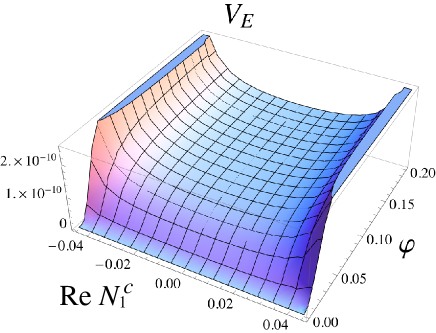
The dynamics of inflation can be studied by examining the steepest descent trajectory of the scalar potential (20). Assuming that inflation takes place in the $L_{k}$-$H_{u}$ D-flat direction along the first generation lepton supermultiplet ($k=1$) and the e-folding number $N_{e}=60$, we find $\xi=1674$ fixed by the CMB power spectrum (procedure explained in the next subsection). It is found numerically that the trajectory is along ${\rm Im}\varphi=0$. We thus consider only the real values of $\varphi$. The inflaton trajectory fluctuates in the directions of $N_{m}^{c}$ as shown in Fig. 1, where the values of the real and imaginary parts of $N_{1}^{c}$ and $N_{2}^{c}$ are plotted along the steepest descent trajectory. The parameter $\zeta$ for the quartic terms in the Kähler potential is chosen to be a moderate value $\zeta=100$ and the field values are measured in the reduced Planck unit $8\pi G=1$. While the trajectory seems rather complicated, inflation actually terminates (that is, one of the slow roll parameters becomes ${{\mathcal{O}}}(1)$) before the complication starts. In the example considered here the slow roll terminates at $\varphi=0.0371$, where $N_{1}^{c}$ and $N_{2}^{c}$ are still stabilised close to $N_{m}^{c}=0$. Fig. 2 shows the shape of the potential as a function of $\varphi$ and ${\rm Re}N_{1}^{c}$, where ${\rm Im}N_{1}^{c}$, ${\rm Re}N_{2}^{c}$, ${\rm Im}N_{2}^{c}$ are taken to be along the trajectory of Fig. 1. In this case the primordial tilt and the tensor-to-scalar ratio of the CMB are computed to be $n_{s}=0.968$, $r=0.00296$. The red spectrum with very small $r$ is typical of the nonminimally coupled Higgs inflation. The horizon exit of the comoving CMB scale takes place at $\varphi=0.318$. In computing the CMB spectrum the rôle played by $\zeta$ is minor, as $\zeta$ has no effects once the inflaton trajectory is stabilised along $N_{m}^{c}\approx 0$.

Figure 1: The steepest descent trajectory of the scalar potential (20), for $M_{1}=M_{2}=10^{13}$ GeV, $a=0$, $b=1$, $\delta=0$, $\sigma=0$ and $k=1$, $\xi=1674$, $\zeta=100$. The red solid, the orange dashed, the green dot-dashed and the blue dotted curves respectively shows the values of ${\rm Re}N_{1}^{c}$, ${\rm Im}N_{1}^{c}$, ${\rm Re}N_{2}^{c}$ and ${\rm Im}N_{2}^{c}$. The slow roll terminates at $\varphi=0.0371$. The field values are measured in the reduced Planck unit $8\pi G=1$.

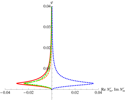
Setting $N_{1}^{c}$, $N_{2}^{c}\rightarrow 0$ and restricting $\varphi$ to take real values, the scalar potential (17) simplifies to

$$V_{F}=\frac{\lambda}{4}\varphi^{4},$$ (22)

where $\lambda\equiv(y_{D}^{\dagger}y_{D})_{kk}$ is the $k$-$k$ component ($k=1,2,3$) of the matrix representation of

$$y_{D}^{\dagger}y_{D}=\frac{2}{v^{2}\sin^{2}\beta}U_{\rm MNS}\sqrt{D_{\nu}}^{T}R^{\dagger}MR\sqrt{D_{\nu}}U_{\rm MNS}^{\dagger}.$$ (23)

The resulting inflationary model is essentially the nonminimally coupled $\lambda\phi^{4}$ model, discussed in Okada et al. (2010). We have analysed the above example (corresponding to $\lambda=(y_{D}^{\dagger}y_{D})_{11}=0.00490$) in this approximation, and found essentially no difference. For example the predictions for $n_{s}$ and $r$ are exactly the same within 3 significant digits. For smaller $M_{m}$ the effects of nonzero $N_{m}^{c}$ become even more negligible, as the slow roll terminates at a larger value of $\varphi$ and the turn around behaviour of $N_{m}^{c}$ occurs at the smaller mass scale of $M_{m}$.

Figure 2: The scalar potential $V_{\rm E}$ as a function of $\varphi$ and ${\rm Re}N_{1}^{c}$. The other fields ${\rm Im}N_{1}^{c}$, ${\rm Re}N_{2}^{c}$, ${\rm Im}N_{2}^{c}$ are chosen to take values along the steepest descent trajectory.

III.3 Cosmological parameters

As the single field approximation $N_{m}^{c}=0$, $\varphi\in{{\mathbb{R}}}$ is sufficiently accurate, we shall study the inflationary dynamics within this approximation. We rescale the inflaton field as

$$\chi={\sqrt{2}}\varphi,$$ (24)

so that the kinetic term is canonically normalised in the Lagrangian

$${{\mathcal{L}}}_{\rm J}=\sqrt{-g_{\rm J}}\left[\frac{1+\xi\chi^{2}}{2}R_{\rm J}-\frac{1}{2}g_{\rm J}^{\mu\nu}\partial_{\mu}\chi\partial_{\nu}\chi-V_{F}\right].$$ (25)

Here the subscript J indicates the Jordan frame and

$$V_{F}=\frac{\lambda}{16}\chi^{4},\quad\xi\equiv\frac{\gamma}{4}-\frac{1}{6}.$$ (26)

This is the Lagrangian in the Jordan frame where the scalar field is nonminimally coupled to the background curvature. The Lagrangian in the Einstein frame is obtained by the Weyl transformation $g^{\rm E}_{\mu\nu}=(1+\xi\chi^{2})g^{\rm J}_{\mu\nu}$. The canonically normalised inflaton field $\hat{\chi}$ in the Einstein frame is related to $\chi$ by

$$d\hat{\chi}=\frac{\sqrt{1+\xi\chi^{2}+6\xi^{2}\chi^{2}}}{1+\xi\chi^{2}}d\chi.$$ (27)

The potential in the Einstein frame is

$$V_{\rm E}=\frac{\lambda}{16}\frac{\chi^{4}}{(1+\xi\chi^{2})^{2}},$$ (28)

in terms of which the slow roll parameters in the Einstein frame are defined as

$$\epsilon=\frac{1}{2}\left(\frac{1}{V_{\rm E}}\frac{dV_{\rm E}}{d\hat{\chi}}\right)^{2},\qquad\eta=\frac{1}{V_{\rm E}}\frac{d^{2}V_{\rm E}}{d\hat{\chi}^{2}}.$$ (29)

The potential $V_{\rm E}$ in the single field approximation (28) is much simpler than the original one (17) and is determined solely by $\lambda=(y_{D}^{\dagger}y_{D})_{kk}$ and $\xi$. For given $\lambda$ and the e-folding number $N_{e}$, the nonminimal coupling $\xi$ is fixed by the CMB power spectrum. For definiteness we use the maximum likelihood value $\Delta^{2}_{R}(k_{0})=2.43\times 10^{-9}$ from the 9-year WMAP data Bennett et al. (2012); Hinshaw et al. (2012), where the calibration is set at $k_{0}=0.002\mbox{ Mpc}^{-1}$. This is related to the power spectrum ${{\mathcal{P}}}_{R}=V_{\rm E}/24\pi^{2}\epsilon$ of the curvature perturbation (at the horizon exit of the comoving scale) by $\Delta_{R}^{2}(k)=\frac{k^{3}}{2\pi^{2}}{{\mathcal{P}}}_{R}(k)$. We denote the value of $\chi$ at the end of the slow roll (characterised by $\max(\epsilon,\eta)=1$) as $\chi=\chi_{*}$, and the value of $\chi$ at the horizon exit of the comoving CMB scale $k$ as $\chi=\chi_{k}$. These are related by the e-folding number through $N_{e}=\int_{\chi_{*}}^{\chi_{k}}d\chi V_{\rm E}({d\hat{\chi}}/{d\chi})/({dV_{\rm E}}/{d\hat{\chi}})$.

From the values of the slow roll parameters at the horizon exit of the comoving CMB scale, the scalar spectral index $n_{s}\equiv d\ln{{\mathcal{P}}}_{R}/d\ln k=1-6\epsilon+2\eta$ and the tensor-to-scalar ratio $r\equiv{{\mathcal{P}}}_{\rm gw}/{{\mathcal{P}}}_{\rm R}=16\epsilon$ can be computed. The results are summarised in Table 1, for $N_{e}=50$, $60$ and several values of $\lambda=(y_{D}^{\dagger}y_{D})_{kk}$. There exists a lower bound on $\lambda$ set by the minimal coupling limit $\xi\rightarrow 0$. In this limit the model reduces to chaotic inflation with the quartic potential $V_{\rm E}=\frac{\lambda}{16}\chi^{4}$, where $\lambda=1.05\times 10^{-12}$ for $N_{e}=50$ and $\lambda=6.19\times 10^{-13}$ for $N_{e}=60$, fixed by the value of ${{\mathcal{P}}}_{R}$. In contrast to the SM Cervantes-Cota and Dehnen (1995); Bezrukov and Shaposhnikov (2008); Barvinsky et al. (2008); De Simone et al. (2009); Bezrukov and Shaposhnikov (2009); Bezrukov et al. (2011); Barvinsky et al. (2009a, b); Barbon and Espinosa (2009); Burgess et al. (2009, 2010); Hertzberg (2010); Lerner and McDonald (2010a, b) and the supersymmetric Einhorn and Jones (2010); Ferrara et al. (2010, 2011); Arai et al. (2011) Higgs inflation models the nonminimal coupling $\xi$ does not need to be large. We see from the table that $\xi\lesssim{{\mathcal{O}}}(1)$ for $\lambda\lesssim 10^{-9}$. Hence, at least for these values of $\lambda$ the model is obviously free from the danger of violating the unitarity bound. Small $\xi$ is also favoured for avoiding large $R$-parity violation, as discussed later in Section VI. The Dirac Yukawa coupling $y_{D}^{mi}$ is related to $a$, $b$, $\delta$, $\sigma$, $M_{1}$, $M_{2}$ through (19). We will discuss the relation between $\lambda$ and these parameters in Section V. Leptogenesis also constrains certain neutrino mass parameters, which will be discussed in Section IV.

$N_{e}$	$\lambda\equiv(y_{D}^{\dagger}y_{D})_{kk}$	$\xi$	$\chi_{*}$	$\chi_{k}$	$n_{s}$	$r$
	$0.1$	6348	0.0135	0.106	0.962	0.00419
	$10^{-3}$	635	0.0426	0.335	0.962	0.00419
	$10^{-5}$	63.4	0.135	1.06	0.962	0.00420
	$10^{-7}$	6.26	0.424	3.33	0.962	0.00430
50	$10^{-9}$	0.555	1.28	9.94	0.961	0.00545
	$10^{-10}$	$0.131$	2.02	15.4	0.961	0.00945
	$10^{-11}$	$0.0188$	2.99	19.5	0.959	0.0379
	$5\times 10^{-12}$	$8.70\times 10^{-3}$	3.21	20.0	0.957	0.0691
	$2\times 10^{-12}$	$2.15\times 10^{-3}$	3.39	20.2	0.951	0.165
	$1.05\times 10^{-12}$	$0$	3.46	20.3	0.942	0.311
	$0.1$	7567	0.0124	0.106	0.968	0.00296
	$10^{-3}$	757	0.0391	0.335	0.968	0.00296
	$10^{-5}$	75.6	0.123	1.06	0.968	0.00297
	$10^{-7}$	7.48	0.389	3.33	0.968	0.00303
	$10^{-9}$	0.676	1.18	10.0	0.968	0.00369
60	$10^{-10}$	0.168	1.90	15.9	0.968	0.00588
	$10^{-11}$	0.0270	2.84	20.8	0.966	0.0203
	$5\times 10^{-12}$	0.0135	3.10	21.5	0.965	0.0356
	$2\times 10^{-12}$	$4.44\times 10^{-3}$	3.32	22.0	0.962	0.0822
	$10^{-12}$	$1.24\times 10^{-3}$	3.42	22.2	0.957	0.161
	$6.19\times 10^{-13}$	$0$	3.46	22.2	0.951	0.260

Table 1: The nonminimal coupling $\xi$, the inflaton values at the end of the slow roll ($\chi_{*}$) and at the horizon exit ($\chi_{k}$), the spectral index $n_{s}$, and the tensor-to-scalar ratio $r$ for e-folding $N_{e}=50$, $60$ and for various different values of $\lambda=(y_{D}^{\dagger}y_{D})_{kk}$. The coupling $\xi$ is fixed by the amplitude of the curvature perturbation. The last lines ($N_{e}=50$, $\lambda=1.05\times 10^{-12}$ and $N_{e}=60$, $\lambda=6.19\times 10^{-13}$) correspond to minimal coupling.

Figure 3: Plot of the scalar spectral index $n_{s}$ and the tensor-to-scalar ratio $r$, with the 68% and 95% confidence level contours from the WMAP9$+$eCMB$+$BAO$+H_{0}$ data Bennett et al. (2012); Hinshaw et al. (2012). Indicated by $\bullet$ are the prediction of our model (NM-$LH_{u}$) for e-folding numbers $N_{e}=50$ and $60$. The coupling $\lambda=(y_{D}^{\dagger}y_{D})_{kk}$ is a diagonal element of (23), which is related to the neutrino mass parameters (see Sec. V). For comparison, the spectra of the Harrison-Zel’dovich (HZ), the $m^{2}\phi^{2}$ minimally coupled chaotic inflation model, as well as the A-term-lifed MSSM flat-direction inflation model (AFD) are also indicated. $\Delta n_{s}$ is the expected Planck accuracy Planck:2006uk (2006); Ade et al. (2011).

III.4 Observational constraints and comparison with other models based on supersymmetric seesaw

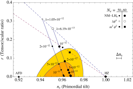
We show in Fig.3 the predicted values of $n_{s}$ and $r$ of our model along with the 68% and 95% confidence level contours from the WMAP9$+$eCMB$+$BAO $+H_{0}$ data Bennett et al. (2012); Hinshaw et al. (2012). The prediction is seen to be consistent with the present data, apart from the regions where the Yukawa coupling is extremely small. The 2-$\sigma$ constraints roughly correspond to $M_{m}\gtrsim$ TeV, details of which depending on the other neutrino mass parameters (see Section V). While the minimally coupled $\lambda\phi^{4}$ model lies outside the 2-$\sigma$ constraints, the nonminimally coupled $\lambda\phi^{4}$, even if the coupling is as small as $\xi\sim 10^{-2}$, sits well inside the 1-$\sigma$ constraints. In the figure we also indicate for comparison the Harrison-Zel’dovich spectrum as well as the spectra of two other inflationary models arising from the supersymmetric seesaw model. These are:

$\tilde{N}_{R}$ chaotic inflation model

— Inflation is driven by a right-handed scalar neutrino, with the seesaw mass scale identified as the inflaton mass Murayama et al. (1993, 1994); Ellis et al. (2004). It is essentially the minimally coupled $m^{2}\phi^{2}$ chaotic inflation model, but has phenomenological advantages such as automatic leptogenesis. The spectrum is marked with $\blacksquare$ in the figure.

A-term inflation model

— This model assumes $u^{c}d^{c}d^{c}$, $e^{c}LL$, or $N_{R}^{c}LH_{u}$ direction of the (singlet-extended) MSSM as the inflaton Allahverdi et al. (2006); Allahverdi et al. (2007a, b); Bueno Sanchez et al. (2007). The A-term inflation model predicts very small $r$ and $n_{s}\approx 1-4/N_{e}$. Since inflation takes place at a low energy scale and the e-folding cannot be large ($N_{e}\lesssim 50$), we show the case for $N_{e}=50$ (thus $n_{s}=0.92$) in the figure, marked with $\blacklozenge$ (AFD) .

In the figure we also indicate the expected resolution $\Delta n_{s}\approx 0.0045$ of the Planck satellite experiments Planck:2006uk (2006); Ade et al. (2011). The data from the Planck satellite is soon to be available. There are more sensitive CMB polarisation experiments planned in the near future Kermish et al. (2012); Hazumi (2008), which we expect will put these models to the test with even higher resolution.

IV Reheating and baryogenesis

The scalar potential (20) has a minimum at $\varphi=N_{m}^{c}=0$ corresponding to the global supersymmetric vacuum. After the slow roll, the inflaton undergoes coherent oscillations about this minimum and decays into the SM particles, followed by thermalisation. The nonminimal coupling can alter the reheating temperature only when $\xi$ is extremely large and the decay rate is very small Bassett and Liberati (1998); Tsujikawa et al. (1999). In the model we are discussing the inflaton is in the $L$-$H_{u}$ direction and the coupling to the SM particles is not small. The nonminimal coupling thus has negligible effects on the reheating process. The upper bound of the reheating temperature can be estimated as $T_{\rm RH}\lesssim 10^{7}$ GeV, assuming the Higgs component decay channel $\varphi\rightarrow b\bar{b}$ in the conservative perturbative decay scenario. The nonperturbative reheating scenario Allahverdi et al. (2011) (with parametric resonance) and/or the (s)lepton component decay may lead to a slightly higher upper bound. Taking into account the effects of the redshift during the time needed for thermalisation, we estimate the reheating temperature of this scenario to be $T_{\rm RH}\approx 10^{5}-10^{7}$ GeV. Below in this section we discuss implication of this reheating temperature on the generation of the baryon asymmetry. The constraints from the R-parity violation will be discussed in Section VI.

The baryon asymmetry (1) can be accounted for by different mechanisms, depending on the seesaw mass scale $M_{m}$. If the mass scale is smaller than the reheating temperature $M_{m}\lesssim T_{\rm RH}$, the right-handed (s)neutrinos thermalise and their decay generates lepton number asymmetry. The lepton number is later converted into the baryon number through the sphaleron process. This mechanism is known as thermal leptogenesis Fukugita and Yanagida (1986). If the seesaw mass scale is larger than the reheating temperature $M_{m}\gtrsim T_{\rm RH}$, on the other hand, the lepton number can be generated by the decay of oscillating sneutrinos Murayama et al. (1993, 1994); Murayama and Yanagida (1994). We call this mechanism nonthermal leptogenesis. The generated lepton number is converted into the baryon number, similarly to the thermal leptogenesis case. In addition, as our model includes the MSSM components, the Affleck-Dine mechanism Affleck and Dine (1985) can be operative. We shall discuss the thermal and the nonthermal leptogenesis in our model below.

IV.1 Thermal leptogenesis

In the leptogenesis scenario the out-of-equilibrium decay of the right-handed (s)neutrinos generates the lepton asymmetry, which is later converted into the baryon asymmetry by the $(B+L)$-violating sphaleron transitions. In the supersymmetric theory the conversion rate is computed to be

$$Y_{B}=-\frac{8N_{f}+4N_{H}}{22N_{f}+13N_{H}}Y_{L}=-\frac{8}{23}Y_{L},$$ (30)

where $Y_{L}$ is the yield (the ratio of the number density to the entropy density) of the leptons, and $N_{f}=3$, $N_{H}=2$ are the number of the fermion families and the number of the Higgs doublets.

In generic scenarios of leptogenesis, generation of sufficient baryon asymmetry requires the reheating temperature to be higher than $10^{9}$ GeV. This is much higher than the reheating temperature of our scenario, and in supersymmetric models the gravitino problem can also be serious. It has been pointed out, however, that if the two right-handed neutrino masses are nearly degenerate the CP-asymmetry parameter is enhanced by resonance effects, making the leptogenesis viable even at lower reheating temperature Pilaftsis (1997); Pilaftsis and Underwood (2004); Flanz et al. (1996). In the following we assume the resonant leptogenesis scenario with nearly degenerate right-handed neutrino masses $M_{1}\approx M_{2}$. Thermalisation of the right-handed neutrinos after reheating also requires $M_{1}$, $M_{2}\lesssim T_{\rm RH}$.

Figure 4: The diagrams contributing to the decay mode $N_{m}\rightarrow\tilde{\ell}+\overline{\widetilde{h}}$.

The decay modes of the right-handed (s)neutrinos are

$$N_{m} \rightarrow \widetilde{\ell}_{j}+\overline{\widetilde{h}},$$

$$N_{m} \rightarrow \ell_{j}+H_{u},$$

$$\widetilde{N_{m}^{c}} \rightarrow \widetilde{\ell}_{j}+H_{u},$$

$$\widetilde{N_{m}^{c}}^{\dagger} \rightarrow \ell_{j}+\overline{\widetilde{h}},$$ (31)

and the CP-asymmetry parameters associated with these processes are defined as

$$\varepsilon_{m} \equiv \frac{\sum_{j}\left[\Gamma(N_{m}\rightarrow\widetilde{\ell}_{j}+\overline{\widetilde{h}})-\Gamma(N_{m}\rightarrow\widetilde{\ell}_{j}^{\dagger}+\widetilde{h})\right]}{\sum_{j}\left[\Gamma(N_{m}\rightarrow\widetilde{\ell}_{j}+\overline{\widetilde{h}})+\Gamma(N_{m}\rightarrow\widetilde{\ell}_{j}^{\dagger}+\widetilde{h})\right]}$$

$$= \frac{\sum_{j}\left[\Gamma(N_{m}\rightarrow\ell_{j}+H_{u})-\Gamma(N_{m}\rightarrow\widetilde{\ell}_{j}+H_{u}^{\dagger})\right]}{\sum_{j}\left[\Gamma(N_{m}\rightarrow\ell_{j}+H_{u})+\Gamma(N_{m}\rightarrow\widetilde{\ell}_{j}+H_{u}^{\dagger})\right]}$$

$$= \frac{\sum_{j}\left[\Gamma(\widetilde{N_{m}^{c}}\rightarrow\widetilde{\ell}_{j}+H_{u})-\Gamma(\widetilde{N_{m}^{c}}^{\dagger}\rightarrow\widetilde{\ell}_{j}^{\dagger}+H_{u}^{\dagger})\right]}{\sum_{j}\left[\Gamma(\widetilde{N_{m}^{c}}\rightarrow\widetilde{\ell}_{j}+H_{u})+\Gamma(\widetilde{N_{m}^{c}}^{\dagger}\rightarrow\widetilde{\ell}_{j}^{\dagger}+H_{u}^{\dagger})\right]}$$

$$= \frac{\sum_{j}\left[\Gamma(\widetilde{N_{m}^{c}}^{\dagger}\rightarrow\ell_{j}+\overline{\widetilde{h}})-\Gamma(\widetilde{N_{m}^{c}}\rightarrow\overline{\ell}_{j}+\widetilde{h})\right]}{\sum_{j}\left[\Gamma(\widetilde{N_{m}^{c}}^{\dagger}\rightarrow\ell_{j}+\overline{\widetilde{h}})+\Gamma(\widetilde{N_{m}^{c}}\rightarrow\overline{\ell}_{j}+\widetilde{h})\right]}.$$

Here, $\widetilde{N_{m}^{c}}$ denotes the right-handed scalar neutrinos, $\widetilde{h}$ denotes the (up-type) higgsinos, and $\ell$, $\widetilde{\ell}$ are the components of the lepton and scalar lepton doublets. We follow the notation of Plumacher (1998). The CP asymmetry parameters are computed from the interference of the tree and one-loop diagrams. In Fig. 4 we show the diagrams contributing to one of the decay modes $N_{m}\rightarrow\tilde{\ell}_{j}+\overline{\widetilde{h}}$. The resulting formula for the CP-asymmetry parameters is

$$\varepsilon_{m}\equiv\sum_{n\neq m}\frac{-{\rm Im}[(y_{D}y_{D}^{\dagger})^{2}_{mn}]}{(y_{D}y_{D}^{\dagger})_{mm}(y_{D}y_{D}^{\dagger})_{nn}}\frac{M_{m}\Gamma_{n}}{M_{n}^{2}}\left(\frac{1}{2}V_{n}+S_{n}\right),$$ (33)

where $\Delta M_{mn}^{2}=M_{m}^{2}-M_{n}^{2}$, and

$$V_{n} = \frac{M_{n}^{2}}{M_{m}^{2}}\ln\left(1+\frac{M_{m}^{2}}{M_{n}^{2}}\right),$$ (34)

$$S_{n} = \frac{M_{n}^{2}\Delta M_{nm}^{2}}{(\Delta M_{nm}^{2})^{2}+M_{m}^{2}\Gamma_{n}^{2}},$$ (35)

corresponding respectively to the vertex corrections (such as the 2nd and 3rd diagrams of Fig. 4) and the self-energy corrections (the 4th and 5th diagrams). The decay width is written as

$$\Gamma_{n}=\frac{(y_{D}y_{D}^{\dagger})_{nn}}{4\pi}{M_{n}}.$$ (36)

The lepton asymmetry $Y_{L}$, and hence the baryon asymmetry through the conversion (30), are found by solving the Boltzmann equations. We summarise the Boltzmann equations and related formulae in the Appendix. Here we discuss the results and features that are relevant to our model. We first notice that the CP phases $\delta$ and $\sigma$ do not affect the baryon asymmetry. This is due to the fact that the MNS matrices cancel in the product of the Yukawa couplings appearing in (33),

$$y_{D}y_{D}^{\dagger}=\frac{2}{v^{2}\sin^{2}\beta}\sqrt{M}R\widetilde{D}_{\nu}R^{\dagger}\sqrt{M}.$$ (37)

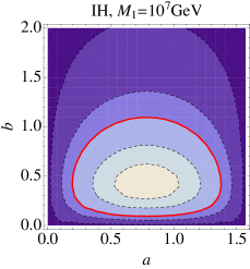
Here, $\widetilde{D}_{\nu}={\rm diag}(m_{2},m_{3})$ for the normal mass hierarchy and $\widetilde{D}_{\nu}={\rm diag}(m_{1},m_{2})$ for the inverted mass hierarchy. The baryon number, on the other hand, depends on the parameters $a$, $b$ in (13), as well as on the right-handed neutrino masses $M_{1}$, $M_{2}$. In Fig.5 we show the yield of the baryon asymmetry $Y_{B}$, as $a$ and $b$ are varied. The left panel shows the result for the normal mass hierarchy with $M_{1}=10^{5}$ GeV, and the right panel is for the inverted mass hierarchy with $M_{1}=10^{7}$ GeV. In both panels the mass difference is chosen to be $M_{2}-M_{1}=10^{-7}\times M_{1}$. The red contour curves indicate $Y_{B}=8.7\times 10^{-11}$ corresponding to the observed value.

The dependance of the baryon asymmetry of the universe on these parameters can be understood as follows. The baryon asymmetry generated through thermal leptogenesis is proportional to the CP violation parameter $\varepsilon_{m}$ as Buchmuller et al. (2002, 2005)

$$Y_{B}\approx\kappa\frac{\varepsilon_{m}}{g_{*}},$$ (38)

where $g_{*}\approx 200$ is the number of degrees of freedom during leptogenesis and $\kappa\lesssim 1$ is the efficiency factor depending on details of the Boltzmann equations. In the resonant leptogenesis with nearly degenerate right-handed neutrino masses $M_{1}\approx M_{2}$ we find $V_{n}\approx\ln 2\ll S_{n}$. The maximal enhancement of the CP asymmetry parameter $\varepsilon_{m}$ occurs when the decay width of either of the right-handed (s)neutrinos becomes close to the mass difference, $\Delta M_{nm}^{2}\approx M_{m}\Gamma_{n}$. Parametrizing the mass difference as $\Delta M_{21}^{2}=\alpha M_{1}\Gamma_{2}$, the CP asymmetry parameters read

$$\varepsilon_{1} \approx -\frac{\alpha}{1+\alpha^{2}}\frac{{\rm Im}\left[(y_{D}y_{D}^{\dagger})_{12}^{2}\right]}{(y_{D}y_{D}^{\dagger})_{11}(y_{D}y_{D}^{\dagger})_{22}},$$

$$\varepsilon_{2} \approx \frac{(\alpha^{2}+1)\Gamma_{1}\Gamma_{2}}{\Gamma_{1}^{2}+\alpha^{2}\Gamma_{2}^{2}}\varepsilon_{1}.$$ (39)

For the (nearly) degenerate right-handed neutrino masses, the matrix $\sqrt{M}$ in (37) becomes proportional to the identity. Then ${\rm Im}\left[(y_{D}y_{D}^{\dagger})_{12}^{2}\right]/(y_{D}y_{D}^{\dagger})_{11}(y_{D}y_{D}^{\dagger})_{22}$ is written as

$$\frac{2(m_{2}^{2}-m_{3}^{2})\sin 2a\sinh 2b}{(m_{2}-m_{3})^{2}\cos^{2}2a-(m_{2}+m_{3})^{2}\cosh^{2}2b}$$ (40)

for the normal mass hierarchy and

$$\frac{2(m_{1}^{2}-m_{2}^{2})\sin 2a\sinh 2b}{(m_{1}-m_{2})^{2}\cos^{2}2a-(m_{1}+m_{2})^{2}\cosh^{2}2b}$$ (41)

for the inverted mass hierarchy. These have maxima at $a=\pi/4\approx 0.785$ and $b=\ln(3+2\sqrt{2})/4\approx 0.441$, with maximal value $(m_{3}-m_{2})/(m_{3}+m_{2})\approx 0.704$ for (40) and $(m_{2}-m_{1})/(m_{2}+m_{1})\approx 7.93\times 10^{-3}$ for (41). Note that $\varepsilon_{m}$ do not depend on the seesaw mass scale $M_{m}$ except through $\alpha$, $\Gamma_{1}$ and $\Gamma_{2}$. By adjusting the parameters $a$, $b$ and $\alpha$ that are not constrained by observation, it is always possible to reproduce the baryon asymmetry $Y_{B}=8.7\times 10^{-11}$.

Figure 5: The neutrino mass parameters $a$ and $b$ yielding the observed value of the baryon asymmetry $Y_{B}=8.7\times 10^{-11}$ (the red contour curves). The left panel shows the case $M_{1}=10^{5}$ GeV with the normal mass hierarchy, and the right panel is for $M_{1}=10^{7}$ GeV with the inverted mass hierarchy. In both panels the contours are $Y_{B}=2\times 10^{-10}$, $1.5\times 10^{-10}$, $8.7\times 10^{-11}$, $5\times 10^{-11}$, $1\times 10^{-11}$ from inside. We have chosen $(M_{2}-M_{1})/M_{1}=10^{-7}$.

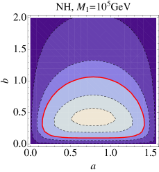
IV.2 Nonthermal leptogenesis due to decaying right-handed scalar neutrinos

The mechanism described above operates when the right-handed neutrino masses $M_{1}$, $M_{2}$ are smaller than the reheating temperature which we assume in our scenario to be in the range $T_{\rm RH}=10^{5}-10^{7}$ GeV. For larger $M_{1}$, $M_{2}$ the thermal leptogenesis scenario is not applicable as the right-handed (s)neutrinos do not thermalise. It is nevertheless possible to generate sufficient baryon asymmetry due to the decay of the right-handed sneutrinos that have acquired expectation values during inflation. In this sense our model is somewhat similar to the inflation model driven by the right-handed scalar neutrinos Murayama et al. (1993, 1994); Ellis et al. (2004). Indeed, for large seesaw scales the right-handed scalar neutrinos have noticeable contribution to the dynamics after the slow-roll, as shown in Fig.1 for $M_{1}=M_{2}=10^{13}$ GeV. Note, however, that the right-handed scalar neutrinos do not have to be involved in the inflationary dynamics.

In the supersymmetric SM including the right-handed neutrinos leptogenesis is automatic as long as the Hubble scale during inflation $H_{\rm inf}$ is larger than the right-handed neutrino mass scale Murayama and Yanagida (1994), which is always the case in our model. Take, for example, the case of $M_{1}=M_{2}=10^{13}$ GeV and $N_{e}=60$ discussed in Section III B, which gives $r=0.00296$. Using the CMB power spectrum $\Delta_{R}^{2}(k_{0})=2.43\times 10^{-9}$, the Hubble parameter during inflation can be expressed in terms of the tensor-to-scalar ratio $r=16\epsilon$ as $H_{\rm inf}=2.67\times\sqrt{r}\times 10^{14}$ GeV. With $r=0.00296$ the Hubble parameter during inflation is larger than the right-handed neutrino masses, $H_{\rm inf}\approx 1.45\times 10^{13}$ GeV $>M_{1}$, $M_{2}$. The seesaw relation (5) with the Yukawa coupling $\lesssim{{\mathcal{O}}}(1)$ constrains $M_{1}$, $M_{2}\lesssim 10^{13}$ GeV, and for smaller $M_{1}$, $M_{2}$ the model yields larger $r$ and hence larger $H_{\rm inf}$, so the inequality $H_{\rm inf}>M_{1}$, $M_{2}$ is satisfied more safely.

In this nonthermal leptogenesis scenario the right-handed scalar neutrinos acquire expectation values $\langle\widetilde{N}\rangle$, either classically by the nontrivial inflaton trajectory, or due to the quantum fluctuation during inflation. This $\langle\widetilde{N}\rangle$ can be regarded as the initial value of the right-handed scalar neutrinos that oscillate and decay. We shall assume $\langle\widetilde{N}\rangle\lesssim M_{\rm Pl}$, where $M_{\rm Pl}$ is the Planck mass. Along with the decay of the right-handed scalar neutrinos the lepton asymmetry is generated, which is later converted into the baryon asymmetry by the $B-L$ conserving sphaleron process. The process of the decay actually depends on the decay rate of the inflaton $\Gamma_{\varphi}$ and that of the right-handed neutrinos $\Gamma_{n}$. When (i) the scalar neutrino decay rate is larger than the inflaton decay rate $\Gamma_{n}>\Gamma_{\varphi}$, the scalar neutrinos decay during the reheating. When (ii) $\Gamma_{n}<\Gamma_{\varphi}<\Gamma_{n}(M_{\rm Pl}/\langle\widetilde{N}\rangle)^{4}$, the scalar neutrinos decay after the reheating but do not dominate the energy density of the universe. When (iii) the scalar neutrino decay rate is much smaller $\Gamma_{\varphi}>\Gamma_{n}(M_{\rm Pl}/\langle\widetilde{N}\rangle)^{4}$, the right-handed scalar neutrinos dominate the universe before they decay. In our model, the scalar neutrino decay rate is (36) and the inflaton decay rate is estimated as $\Gamma_{\varphi}\approx 4$ MeV, assuming the Higgs $\rightarrow b\bar{b}$ decay channel and the Higgs mass $\approx$ 125 GeV. It can be shown that in our scenario the case (iii) never occurs, as long as the inflaton trajectory is controlled to be nearly straight by the noncanonical Kähler terms. The threshold between (i) and (ii) is around $M_{1}\approx M_{2}\approx 10^{6.5}$ GeV, for typical values of the mass parameters $a=b=1$ and for the normal or inverted mass hierarchy.

In both (i) and (ii) cases the yield of the lepton asymmetry is estimated as Murayama and Yanagida (1994)

$$Y_{L}=\varepsilon_{m}\frac{\langle\widetilde{N}\rangle^{2}}{M_{m}M_{\rm Pl}}\left(\frac{\Gamma_{\varphi}}{M_{\rm Pl}}\right)^{\frac{1}{2}},$$ (42)

and the baryon asymmetry follows from (30). Assuming

$$\langle\widetilde{N}\rangle^{2}\simeq\frac{3H_{\rm inf}^{4}}{8\pi^{2}M_{m}^{2}}$$ (43)

generated by the quantum fluctuations, the observed baryon asymmetry (1) with the condition for the CP asymmetry parameter $|\varepsilon_{m}|\lesssim 1$ leads to a mild upper bound on the seesaw mass scale $M_{m}\lesssim 10^{12}$ GeV.

V The inflaton self coupling and the neutrino mass parameters

Our model of inflation is well approximated by the nonminimally coupled single field $\lambda\phi^{4}$ model. We have seen in Section III that the inflaton self coupling $\lambda=(y_{D}^{\dagger}y_{D})_{kk}$ is related to the CMB spectrum, and argued that in the near future the value of $\lambda$ will be constrained more severely by the observation. As $\lambda$ is constructed from components of the Dirac Yukawa coupling, it is determined by the neutrino mass parameters. In this section we describe the relation between $\lambda$ and these parameters.

We shall assume nearly degenerate right-handed neutrino mass parameters $M_{1}\approx M_{2}$, which is favoured for successful thermal leptogenesis as we discussed in the previous section. The matrix $M={\rm diag}(M_{1},M_{2})$ is then proportional to the identity matrix and the relation (23) becomes

$$y_{D}^{\dagger}y_{D}\approx\frac{2M_{1}}{v^{2}\sin^{2}\beta}U_{\rm MNS}\sqrt{D_{\nu}}^{T}R^{\dagger}R\sqrt{D_{\nu}}U_{\rm MNS}^{\dagger}.$$ (44)

Thus $(y_{D}^{\dagger}y_{D})_{kk}$ is proportional to the seesaw mass parameter $M_{1}$. Essentially, the inflaton self coupling is determined by the seesaw mass scale Arai et al. (2012). Further complexity arises from the dependence on the other parameters $b$, $\delta$ and $\sigma$, which are not constrained by the present observation.

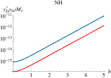
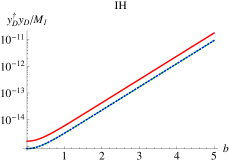
Dependence on $a$ and $b$. — We first notice that $\lambda$ does not depend on the parameter $a$. This is easily seen, as the product $R^{\dagger}R$ appearing in (44) is written as

$$R^{\dagger}R=\left(\begin{array}[]{cc}\cosh 2b&i\sinh 2b\\ -i\sinh 2b&\cosh 2b\\ \end{array}\right).$$ (45)

The coupling $\lambda$ monotonically increases with $b>0$. We show the behaviour of $(y_{D}^{\dagger}y_{D})_{kk}/M_{1}$ as functions of $b$ in Fig. 6, for $k=1,2,3$, with the CP violating phases set to be $\delta=0$, $\sigma=0$. The self coupling $\lambda$ changes by an order as $b$ is shifted by 1; the dependence on $b$ is thus significant.

Figure 6: Plot of $\lambda/M_{1}\equiv(y_{D}^{\dagger}y_{D})_{kk}/M_{1}$ (in GeV^-1) as functions of $b$. The Dirac and Majorana phases are chosen to be zero. The left panel is for the normal mass hierarchy and the right is for the inverted mass hierarchy. On each panel, the red solid, the green dashed, and the blue dotted curves indicate $k=1,2,3$, respectively. The $k=2$ and $k=3$ curves overlie each other.

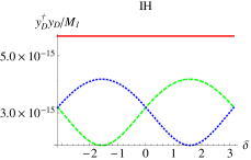
Dependence on the Dirac phase $\delta$. — The dependence of the inflaton self coupling $\lambda$ on the Dirac phase $\delta$ is shown in Fig. 7, where $(y_{D}^{\dagger}y_{D})_{kk}/M_{1}$ is plotted for $-\pi\leq\delta<\pi$. We have chosen $b=1$ and $\sigma=0$. In the case of the normal mass hierarchy the $k=1$ component is more susceptible than $k=2,3$, whereas for the inverted mass hierarchy $k=2,3$ are more susceptible than $k=1$.

Figure 7: Plot of $\lambda/M_{1}\equiv(y_{D}^{\dagger}y_{D})_{kk}/M_{1}$ for $k=1$ (the red solid curves), $k=2$ (green dashed) and $k=3$ (blue dotted), as functions of the Dirac phase $\delta$. The unit of $\lambda/M_{1}$ is in GeV^-1. The left panel shows the case for the normal mass hierarchy and the right panel is for the inverted mass hierarchy. We have chosen $b=1$ and $\sigma=0$.

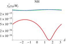
Dependence on the Majorana phase $\sigma$. — The inflaton self coupling $\lambda$ also depends on the Majorana phase $\sigma$. In Fig. 8 we show the behaviour of $(y_{D}^{\dagger}y_{D})_{kk}/M_{1}$ as $\sigma$ is varied from $-\pi$ to $\pi$. We have chosen $b=1$ and $\delta=0$.

Figure 8: Plot of $\lambda/M_{1}\equiv(y_{D}^{\dagger}y_{D})_{kk}/M_{1}$ for $k=1$ (the red solid curves), $k=2$ (green dashed), $k=3$ (blue dotted), as functions of the Majorana phase $\sigma$. The unit of $\lambda/M_{1}$ is in GeV^-1. The left panel shows the case for the normal mass hierarchy and the right panel is for the inverted mass hierarchy. We have chosen $b=1$ and $\delta=0$.

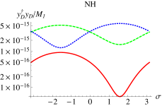
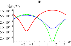
To summarise, the inflaton self coupling $\lambda$ depends on $b$, $\delta$ and $\sigma$ but not on $a$. These parameters are not constrained by present experiments and thus introduce ambiguity in prediction of the model. Consider for instance the 2-$\sigma$ contour in Fig.3. For $N_{e}=60$ this gives a constraint $\lambda=(y_{D}^{\dagger}y_{D})_{kk}\gtrsim 10^{-12}$ which corresponds to $M_{1}\approx M_{2}\gtrsim 2$ TeV for $b=1$, $\delta=\sigma=0$, $k=1$ in the normal mass hierarchy (Fig.7). If we take $\delta=1.6$ instead of $\delta=0$, the $2$-$\sigma$ of CMB gives $M_{1}\approx M_{2}\gtrsim 20$ TeV.

VI The effects of R-parity violation

While the seesaw model superpotential (2) preserves the R-parity (assuming the odd parity for the right-handed neutrino superfield), the Kähler potential (16) breaks it by the $\gamma_{i}L_{i}H_{u}$ terms. Small R-parity violation is known to be harmless, and it can often be beneficial Dreiner (1997); Barbier et al. (2005); Buchmuller et al. (2007). It can nevertheless lead to difficulties and the consequences of introducing such terms need to be checked carefully. In this section we discuss viability of the scenario focusing on the effects of R-parity violation. We assume the canonical form of the Kähler terms for all the other chiral multiplets.

An immediate consequence of the $\gamma_{i}L_{i}H_{u}$ terms in the Kähler potential is that the the Lagrangian includes the following terms:

$${{\mathcal{L}}} \supset \int d^{4}\theta\phi^{\dagger}\phi\left(L_{i}^{\dagger}L_{i}+H_{u}^{\dagger}H_{u}+\gamma_{i}L_{i}H_{u}+h.c.\right)$$ (46)

$$= \int d^{4}\theta\left(L_{i}^{\dagger}L_{i}+H_{u}^{\dagger}H_{u}+\frac{\phi^{\dagger}}{\phi}\gamma_{i}L_{i}H_{u}+h.c.\right),$$

where $\phi$ is the compensator in the superconformal formalism. To go from the first to the second line we have rescaled $L_{i},H_{u}\rightarrow\phi^{-1}L_{i},\phi^{-1}H_{u}$. When the supersymmetry is broken the compensator acquires an expectation value $\langle\phi\rangle=1+\theta^{2}F_{\phi}$, where $F_{\phi}$ is the compensator F-term. The third term in (46) then becomes $\int d^{4}\theta(1+\overline{\theta}^{2}F_{\phi}^{\dagger})(1-\theta^{2}F_{\phi})\gamma_{i}L_{i}H_{u}$. This suggests generation of a bilinear R-parity breaking term $W_{\not R}=F_{\phi}^{\dagger}\gamma_{i}L_{i}H_{u}\equiv\mu_{i}L_{i}H_{u}$, as well as an R-parity breaking B-term $-|F_{\phi}|^{2}\gamma_{i}\tilde{\ell}_{i}h_{u}$. In generic scenarios of supersymmetry breaking the compensator F-term gives rise to the gravitino mass, $F_{\phi}\approx m_{3/2}$. Recalling that $\gamma_{i}=\gamma$ is related to the nonminimal coupling $\xi$ by $\xi=\frac{\gamma}{4}-\frac{1}{6}$, we see $\gamma\approx 4\xi\gg 1$ when $\xi\gg 1$ and $\gamma\sim{{\mathcal{O}}}(1)$ when $\xi\lesssim 1$. We will assume $\gamma\sim{{\mathcal{O}}}(1)$ below, as one of the merits of our model was that the extremely large nonminimal coupling that could lead to the unitarity violation can be avoided. The bilinear R-parity breaking term can then be written as $W_{\not R}\sim m_{3/2}\gamma_{i}L_{i}H_{u}\sim m_{3/2}L_{k}H_{u}.$

In the presence of the bilinear R-parity violating terms $W\sim H_{u}(\mu H_{d}+m_{3/2}L_{k})$ the lepton number violating superpotential

$$W_{\Delta L=1}\sim(y_{e}^{ij}\varepsilon^{k})e_{i}^{c}L_{j}L_{k}+(y_{d}^{ij}\varepsilon^{k})d_{i}^{c}Q_{j}L_{k},$$ (47)

where $\varepsilon^{k}\sim m_{3/2}/\mu$, is generated. The cosmological constraints for these effective Yukawa couplings are Campbell et al. (1991); Fischler et al. (1991); Dreiner and Ross (1993)

$$y_{e}^{ij}\varepsilon^{k},\quad y_{d}^{ij}\varepsilon^{k}\lesssim 10^{-7},$$ (48)

from which one obtains $\varepsilon^{k}\sim m_{3/2}/\mu\lesssim 10^{-5}\cos\beta\sim 10^{-6}$. For a typical value of the MSSM $\mu$ parameter $\mu\sim 1$ TeV the gravitino mass of our model is

$$m_{3/2}\lesssim 1\mbox{ MeV}.$$ (49)

Thus, supersymmetry breaking mechanisms consistent with our scenario are those giving a small gravitino mass (such as the gauge mediation scenario). Note that the gravitinos with the small mass (49) are still a good candidate for the cold dark matter, even though the R-parity is broken.

The abundance of the thermally produced gravitinos is calculated as Bolz et al. (2001); Pradler and Steffen (2007); Steffen (2006)

$$\Omega_{\widetilde{G}}h^{2}\simeq 0.3\times\left(\frac{T_{\rm RH}}{10^{10}\mbox{ GeV}}\right)\left(\frac{100\mbox{ GeV}}{m_{3/2}}\right)\left(\frac{M_{\widetilde{g}}}{1\mbox{ TeV}}\right)^{2},$$ (50)

where $h$ is the Hubble parameter in the unit of $100$ km Mpc^-1 s^-1 and $M_{\widetilde{g}}$ is the running gluino mass. With $m_{3/2}\approx 1$ MeV and $M_{\widetilde{g}}\approx 1$ TeV, the condition for avoiding the overdominance $\Omega_{\widetilde{G}}h^{2}\lesssim 0.1$ yields the upper bound of the reheating temperature $T_{\rm RH}\lesssim 10^{5}$ GeV. In a previous section we estimated the reheating temperature be $T_{\rm RH}\approx 10^{5}-10^{7}$ GeV, assuming the decay channel Higgs $\rightarrow b\bar{b}$. The constraint of the gravitino abundance (50) suggests that $T_{\rm RH}\approx 10^{5}$ GeV is favoured. Taking into account the Hubble expansion for the time needed for thermalisation, $T_{\rm RH}\sim 10^{5}$ GeV seems to be a reasonable reheating temperature of our scenario. To summarise, our model typically predicts a scenario of gravitino cold dark matter with the reheating temperature $T_{\rm RH}\sim 10^{5}$ GeV. The smallness of the R-parity violating terms (48) guarantees that the baryon asymmetry generated by thermal/nonthermal leptogenesis remains without being wiped out.

We close this section with two comments. First, the constraint on the R-parity violation (48) does not have to be taken too strict since, for example, details of the flavour structure may slightly relax this condition Endo et al. (2010). Our second comment concerns the effects on the neutrino masses. R-parity violation induces neutrino masses without invoking right-handed neutrinos Hall and Suzuki (1984); Lee (1984a, b); Dawson (1985); Aulakh and Mohapatra (1982); Ellis et al. (1985). This alternative mechanism to the seesaw can be a potential threat, since if such an effect dominates over the usual seesaw mechanism that would give unacceptably large neutrino masses. A back-of-the-envelope calculation shows that there is actually no such danger, as the constraint (48) is more stringent than the one coming from the neutrino masses. For example, in the bilinear R-parity breaking scenario Hempfling (1996); Nilles and Polonsky (1997); Hirsch et al. (2000) the condition on the bilinear coefficient $\mu_{i}$ for not generating too large neutrino masses is $\mu_{i}/\mu\lesssim 10^{-3}\gg 10^{-6}$.

VII Discussion

We have discussed in this paper a simple model of inflationary cosmology based on the supergravity-embedded minimal seesaw model. The scenario is economical as it simultaneously explains various issues – neutrino oscillation, the origin of the baryon asymmetry and the origin of the cold dark matter – apart from the standard issues of big bang cosmology solved by inflation. We have shown that the model reproduces observationally acceptable values of the cosmological parameters, and argued that the prediction for $n_{s}$, $r$ of the CMB spectrum will be tested by satellite experiments in the near future. A particularly interesting feature of this model is that the seesaw mass scale is constrained by the CMB. Thus far useful constraints on the (left-handed) neutrinos, such as the total neutrino masses $\sum m_{\nu}$ and the effective number of the neutrino species, have been obtained by observing the CMB and the large scale structure. However, the nature of the right-handed neutrons remains mysterious: being gauge singlets, their detection in colliders is virtually impossible, nevertheless they are essential for both seesaw mechanism and leptogenesis. In our proposal, the CMB may provide access to the physics of the right-handed neutrinos.

A key feature of our model is the nonminimal coupling of the D-flat direction inflaton to the background gravitational curvature, which is naturally implemented by supergravity embedding of the SM. In contrast to the nonmimimally coupled Higgs inflation type models, the coupling in our case need not be large. This is related to the fact that the Dirac Yukawa coupling can be very small. Such extremely small Yukawa coupling is, nevertheless, not unnatural. The Dirac Yukawa coupling corresponding to a TeV scale right-handed neutrino mass in our model is in the same order as the electron Yukawa coupling. As Nature allows such a small coupling for the electrons, there is no reason to exclude the Dirac Yukawa coupling of the same order for the neutrinos.

Finally, we comment on extension of our model in various directions. While embedding into the $SO(10)$ grand unified theory is not possible, one may for example consider our scenario in the grand unified theory of $SU(5)$ plus a singlet. Also, type III seesaw with $SU(5)$ adjoint neutrinos in $SU(5)$ is possible. It is also straightforward to extend our model to the right-handed neutrinos with three families. An obvious drawback of such an extension is that the inflationary scenario will contain more unconstrained parameters and the predictive power of the model will be reduced.

Acknowledgments

S.K. acknowledges helpful conversations with Alejandro Ibarra, Shinta Kasuya, Kazunori Kohri and Masahide Yamaguchi. This research was supported in part by the Research Program MSM6840770029 the project of International Cooperation ATLAS-CERN of the Ministry of Education, Youth and Sports of Czech Republic, the JSPS - ASCR Japan - Czech Republic Research Cooperative Program (M.A.), the National Research Foundation of Korea Grant-in-Aid for Scientific Research No. 2012-007575 (S.K.) and by the DOE Grant No. DE-FG02-10ER41714 (N.O.). A part of the numerical computation was carried out using computing facilities at the Yukawa Institute, Kyoto University.

Appendix A Boltzmann equations

We discussed leptogenesis within our inflationary scenario in Sec. IV.1 and presented the solutions of the Boltzmann equations. In this appendix we collect related formulae. The Boltzmann equations in the context of leptogenesis are discussed in Kolb and Wolfram (1980); Dolgov and Zeldovich (1981); Luty (1992). We follow the conventions of Plumacher (1998).

In the supersymmetric minimal seesaw model the dominant processes for generating the lepton number are the decay of the right-handed Majorana neutrino $N_{m}$ into the up-type Higgs boson and a lepton, or into the higgsino and a scalar lepton:

$$N_{m}\rightarrow H_{u}+\ell,\quad\overline{\tilde{h}}+\tilde{\ell},$$ (51)

as well as the decay of its superpartner $\widetilde{N_{j}^{c}}$ into the higgsino and a lepton, or into the Higgs boson and a scalar lepton:

$$\widetilde{N_{m}^{c}}\rightarrow H_{u}+\tilde{\ell},\quad\tilde{h}+\overline{\ell}.$$ (52)

The decay widths for these processes are

$$\Gamma_{m}=\frac{M_{m}}{4\pi}(y_{D}y_{D}^{\dagger})_{mm}.$$ (53)

It is convenient to parametrize the inverse temperature using the right-handed neutrino mass $M_{1}$ as

$$z\equiv\frac{M_{1}}{T}.$$ (54)

In the out-of-equilibrium decay of the right-handed neutrinos and sneutrinos, we assume the initial number densities of the leptons $Y_{L_{f}}$ and sleptons $Y_{L_{s}}$ to be zero. We also assume that the right-handed sneutrinos are initially symmetric: $Y_{\widetilde{N_{m}^{c}}}=Y_{\widetilde{N_{m}^{c}}^{\dagger}}$. Ignoring subdominant processes, it follows that $Y_{\widetilde{N_{m}^{c}}}=Y_{\widetilde{N_{m}^{c}}^{\dagger}}$ persists during the subsequent evolution. The Boltzmann equations for the number densities of the right-handed (s)neutrinos and the (s)lepton numbers then read

$$\frac{dY_{N_{m}}}{dz} = -\frac{z}{sH(M_{1})}\left(\frac{Y_{N_{m}}}{Y_{N_{m}}^{\rm eq}}-1\right)\gamma_{N_{m}},$$ (55)

$$\frac{dY_{\widetilde{N}_{m}^{c}}}{dz} = -\frac{z}{sH(M_{1})}\left(\frac{Y_{\widetilde{N}_{m}^{c}}}{Y_{\widetilde{N}_{m}^{c}}^{\rm eq}}-1\right)\gamma_{N_{m}},$$ (56)

$$\frac{dY_{L_{f}}}{dz} = -\frac{z}{sH(M_{1})}\sum_{m}\Big{\{}\left(\frac{1}{2}\frac{Y_{L_{f}}}{Y_{\ell}^{\rm eq}}+\varepsilon_{m}\right)\gamma_{N_{m}}$$ (57)

$$\qquad-\frac{1}{2}\left(\frac{Y_{N_{m}}}{Y_{N_{m}}^{\rm eq}}+\frac{Y_{\widetilde{N}_{m}^{c}}}{Y_{\widetilde{N}_{m}^{c}}^{\rm eq}}\right)\varepsilon_{m}\gamma_{N_{m}}\Big{\}},$$

$$\frac{dY_{L_{s}}}{dz} = -\frac{z}{sH(M_{1})}\sum_{m}\Big{\{}\left(\frac{1}{2}\frac{Y_{L_{s}}}{Y_{\widetilde{\ell}}^{\rm eq}}+\varepsilon_{m}\right)\gamma_{N_{m}}$$ (58)

$$\qquad-\frac{1}{2}\left(\frac{Y_{N_{m}}}{Y_{N_{m}}^{\rm eq}}+\frac{Y_{\widetilde{N}_{m}^{c}}}{Y_{\widetilde{N}_{m}^{c}}^{\rm eq}}\right)\varepsilon_{m}\gamma_{N_{m}}\Big{\}}.$$

Here, $H(M_{1})$ is the Hubble parameter at temperature $T=M_{1}$ and

$$\gamma_{N_{m}}=n_{N_{m}}^{\rm eq}\frac{K_{1}(z)}{K_{2}(z)}\Gamma_{m}$$ (59)

is the reaction density of the decay processes. $K_{1}$, $K_{2}$ are the elliptic integrals of the first and the second kind. The Boltzmann equations (55) and (56), (57) and (58) are identical due to supersymmetry.

We solved the above equations with the yields in equilibrium,

$$Y_{N_{m}}^{\rm eq} = Y_{\widetilde{N}_{m}^{c}}^{\rm eq}=\frac{n_{N_{m}}^{\rm eq}}{s},\quad n_{N_{m}}^{\rm eq}=\frac{M_{1}^{3}}{\pi^{2}z}K_{2}(z),$$ (60)

$$Y_{\ell}^{\rm eq} = Y_{\widetilde{\ell}}^{\rm eq}=\frac{n_{\ell}^{\rm eq}}{s},\quad n_{\ell}^{\rm eq}=\frac{2}{\pi^{2}}\left(\frac{M_{1}}{z}\right)^{3}.$$ (61)

These Boltzmann equations assume supersymmetry and are not strictly applicable below the supersymmetry breaking scale $T\sim$ TeV. The deviation from the supersymmetric case is however expected to be minor as it should naturally be within a factor of 2.

References

- McAllister and Silverstein (2008) L. McAllister and E. Silverstein, Gen.Rel.Grav. 40, 565 (2008), eprint 0710.2951.
- Ashtekar and Singh (2011) A. Ashtekar and P. Singh, Class.Quant.Grav. 28, 213001 (2011), eprint 1108.0893.
- Heckman et al. (2010) J. J. Heckman, A. Tavanfar, and C. Vafa, JHEP 1004, 054 (2010), eprint 0812.3155.
- Bennett et al. (2012) C. Bennett, D. Larson, J. Weiland, N. Jarosik, G. Hinshaw, et al. (2012), eprint 1212.5225.
- Hinshaw et al. (2012) G. Hinshaw, D. Larson, E. Komatsu, D. Spergel, C. Bennett, et al. (2012), eprint 1212.5226.
- Cervantes-Cota and Dehnen (1995) J. L. Cervantes-Cota and H. Dehnen, Nucl. Phys. B442, 391 (1995), eprint astro-ph/9505069.
- Bezrukov and Shaposhnikov (2008) F. L. Bezrukov and M. Shaposhnikov, Phys. Lett. B659, 703 (2008), eprint 0710.3755.
- Barvinsky et al. (2008) A. Barvinsky, A. Kamenshchik, and A. Starobinsky, JCAP 0811, 021 (2008), eprint 0809.2104.
- De Simone et al. (2009) A. De Simone, M. P. Hertzberg, and F. Wilczek, Phys. Lett. B678, 1 (2009), eprint 0812.4946.
- Bezrukov and Shaposhnikov (2009) F. Bezrukov and M. Shaposhnikov, JHEP 07, 089 (2009), eprint 0904.1537.
- Bezrukov et al. (2011) F. Bezrukov, A. Magnin, M. Shaposhnikov, and S. Sibiryakov, JHEP 1101, 016 (2011), eprint 1008.5157.
- Barvinsky et al. (2009a) A. O. Barvinsky, A. Y. Kamenshchik, C. Kiefer, A. A. Starobinsky, and C. Steinwachs, JCAP 0912, 003 (2009a), eprint 0904.1698.
- Barvinsky et al. (2009b) A. Barvinsky, A. Kamenshchik, C. Kiefer, A. Starobinsky, and C. Steinwachs (2009b), eprint 0910.1041.
- Barbon and Espinosa (2009) J. L. F. Barbon and J. R. Espinosa, Phys. Rev. D79, 081302 (2009), eprint 0903.0355.
- Burgess et al. (2009) C. P. Burgess, H. M. Lee, and M. Trott, JHEP 09, 103 (2009), eprint 0902.4465.
- Burgess et al. (2010) C. P. Burgess, H. M. Lee, and M. Trott, JHEP 07, 007 (2010), eprint 1002.2730.
- Hertzberg (2010) M. P. Hertzberg, JHEP 11, 023 (2010), eprint 1002.2995.
- Lerner and McDonald (2010a) R. N. Lerner and J. McDonald, JCAP 1004, 015 (2010a), eprint 0912.5463.
- Lerner and McDonald (2010b) R. N. Lerner and J. McDonald, Phys. Rev. D82, 103525 (2010b), eprint 1005.2978.
- Starobinsky (1980) A. A. Starobinsky, Phys.Lett. B91, 99 (1980).
- Spokoiny (1984) B. Spokoiny, Phys.Lett. B147, 39 (1984).
- Futamase and Maeda (1989) T. Futamase and K.-i. Maeda, Phys. Rev. D39, 399 (1989).
- Salopek et al. (1989) D. S. Salopek, J. R. Bond, and J. M. Bardeen, Phys. Rev. D40, 1753 (1989).
- Makino and Sasaki (1991) N. Makino and M. Sasaki, Prog. Theor. Phys. 86, 103 (1991).
- Aad et al. (2012) G. Aad et al. (ATLAS Collaboration), Phys.Lett. B716, 1 (2012), eprint 1207.7214.
- Chatrchyan et al. (2012) S. Chatrchyan et al. (CMS Collaboration), Phys.Lett. B716, 30 (2012), eprint 1207.7235.
- Ferrara et al. (2010) S. Ferrara, R. Kallosh, A. Linde, A. Marrani, and A. Van Proeyen, Phys. Rev. D82, 045003 (2010), eprint 1004.0712.
- Ferrara et al. (2011) S. Ferrara, R. Kallosh, A. Linde, A. Marrani, and A. Van Proeyen, Phys. Rev. D83, 025008 (2011), eprint 1008.2942.
- Einhorn and Jones (2010) M. B. Einhorn and D. R. T. Jones, JHEP 03, 026 (2010), eprint 0912.2718.
- Arai et al. (2011) M. Arai, S. Kawai, and N. Okada, Phys.Rev. D84, 123515 (2011), eprint 1107.4767.
- Einhorn and Jones (2012) M. B. Einhorn and D. T. Jones, JCAP 1211, 049 (2012), eprint 1207.1710.
- Pallis and Toumbas (2011) C. Pallis and N. Toumbas, JCAP 1102, 019 (2011), eprint 1101.0325.
- (33) P. Minkowski, Phys. Lett. B67, 421 (1977); T. Yanagida (1979), in Proc. of the Workshop on the Baryon Number of the Universe and Unified Theories, Tsukuba, Japan, 13-14 Feb1979, O. Sawada and A. Sugamoto (eds.), KEK report KEK-79-18, p.95; M. Gell-Mann, P. Ramond, and R. Slansky, pp. 315–321 (1979), in Supergravity, P. van Nieuwenhuizen, D.Z. Freedman (eds.), North Holland Publ. Co., 1979, print-80-0576 (CERN); R. N. Mohapatra and G. Senjanovic, Phys.Rev.Lett. 44, 912 (1980).
- Arai et al. (2012) M. Arai, S. Kawai, and N. Okada, Phys.Rev. D86, 063507 (2012), eprint 1112.2391.
- Frampton et al. (2002) P. Frampton, S. Glashow, and T. Yanagida, Phys.Lett. B548, 119 (2002), eprint hep-ph/0208157.
- Murayama et al. (1993) H. Murayama, H. Suzuki, T. Yanagida, and J. Yokoyama, Phys.Rev.Lett. 70, 1912 (1993).
- Murayama et al. (1994) H. Murayama, H. Suzuki, T. Yanagida, and J. Yokoyama, Phys.Rev. D50, 2356 (1994), eprint hep-ph/9311326.
- Ellis et al. (2004) J. R. Ellis, M. Raidal, and T. Yanagida, Phys. Lett. B581, 9 (2004), eprint hep-ph/0303242.
- Allahverdi et al. (2006) R. Allahverdi, K. Enqvist, J. Garcia-Bellido, and A. Mazumdar, Phys. Rev. Lett. 97, 191304 (2006), eprint hep-ph/0605035.
- Allahverdi et al. (2007a) R. Allahverdi, K. Enqvist, J. Garcia-Bellido, A. Jokinen, and A. Mazumdar, JCAP 0706, 019 (2007a), eprint hep-ph/0610134.
- Allahverdi et al. (2007b) R. Allahverdi, A. Kusenko, and A. Mazumdar, JCAP 0707, 018 (2007b), eprint hep-ph/0608138.
- Bueno Sanchez et al. (2007) J. Bueno Sanchez, K. Dimopoulos, and D. H. Lyth, JCAP 0701, 015 (2007), eprint hep-ph/0608299.
- Fukugita and Yanagida (1986) M. Fukugita and T. Yanagida, Phys.Lett. B174, 45 (1986).
- Flanz et al. (1996) M. Flanz, E. A. Paschos, U. Sarkar, and J. Weiss, Phys.Lett. B389, 693 (1996), eprint hep-ph/9607310.
- Pilaftsis (1997) A. Pilaftsis, Phys. Rev. D56, 5431 (1997), eprint hep-ph/9707235.
- Pilaftsis and Underwood (2004) A. Pilaftsis and T. E. J. Underwood, Nucl. Phys. B692, 303 (2004), eprint hep-ph/0309342.
- Nakamura et al. (2010) K. Nakamura et al. (Particle Data Group), J. Phys. G37, 075021 (2010).
- An et al. (2012) F. An et al. (DAYA-BAY Collaboration), Phys.Rev.Lett. 108, 171803 (2012), eprint 1203.1669.
- Casas and Ibarra (2001) J. Casas and A. Ibarra, Nucl.Phys. B618, 171 (2001), eprint hep-ph/0103065.
- Ibarra and Ross (2004) A. Ibarra and G. G. Ross, Phys.Lett. B591, 285 (2004), eprint hep-ph/0312138.
- (51) M. Kaku, P. K. Townsend, and P. van Nieuwenhuizen, Phys. Rev. D17, 3179 (1978); W. Siegel and S. J. Gates, Jr., Nucl. Phys. B147, 77 (1979); E. Cremmer, S. Ferrara, L. Girardello, and A. Van Proeyen, Nucl. Phys. B212, 413 (1983); S. Ferrara, L. Girardello, T. Kugo, and A. Van Proeyen, Nucl. Phys. B223, 191 (1983); T. Kugo and S. Uehara, Nucl. Phys. B222, 125 (1983a); ibid. B226, 49 (1983b); Prog. Theor. Phys. 73, 235 (1985).
- Okada et al. (2010) N. Okada, M. U. Rehman, and Q. Shafi, Phys.Rev. D82, 043502 (2010), eprint 1005.5161.
- (53) (Planck Collaboration) (2006), eprint astro-ph/0604069, URL http://www.rssd.esa.int/index.php?project=Planck.
- Ade et al. (2011) P. Ade et al. (Planck Collaboration), Astron.Astrophys. 536, 16464 (2011), eprint 1101.2022.
- (55) S. Hotchkiss, A. Mazumdar, and S. Nadathur, JCAP 1106, 002 (2011), eprint 1101.6046; A. Mazumdar and S. Morisi, Phys.Rev. D86, 045031 (2012), eprint 1201.6189.
- Kermish et al. (2012) Z. Kermish, P. Ade, A. Anthony, K. Arnold, K. Arnold, et al. (2012), eprint 1210.7768.
- Hazumi (2008) M. Hazumi, AIP Conf.Proc. 1040, 78 (2008).
- Bassett and Liberati (1998) B. A. Bassett and S. Liberati, Phys.Rev. D58, 021302 (1998), eprint hep-ph/9709417.
- Tsujikawa et al. (1999) S. Tsujikawa, K.-i. Maeda, and T. Torii, Phys.Rev. D60, 063515 (1999), eprint hep-ph/9901306.
- Allahverdi et al. (2011) R. Allahverdi, A. Ferrantelli, J. Garcia-Bellido, and A. Mazumdar, Phys.Rev. D83, 123507 (2011), eprint 1103.2123.
- Murayama and Yanagida (1994) H. Murayama and T. Yanagida, Phys. Lett. B322, 349 (1994), eprint hep-ph/9310297.
- Affleck and Dine (1985) I. Affleck and M. Dine, Nucl. Phys. B249, 361 (1985).
- Plumacher (1998) M. Plumacher, Nucl.Phys. B530, 207 (1998), eprint hep-ph/9704231.
- Buchmuller et al. (2002) W. Buchmuller, P. Di Bari, and M. Plumacher, Nucl.Phys. B643, 367 (2002), eprint hep-ph/0205349.
- Buchmuller et al. (2005) W. Buchmuller, P. Di Bari, and M. Plumacher, Annals Phys. 315, 305 (2005), eprint hep-ph/0401240.
- Gonzalez Felipe et al. (2004) R. Gonzalez Felipe, F. Joaquim, and B. Nobre, Phys.Rev. D70, 085009 (2004), eprint hep-ph/0311029.
- Okada et al. (2012) N. Okada, Y. Orikasa, and T. Yamada, Phys.Rev. D86, 076003 (2012), eprint 1207.1510.
- Dreiner (1997) H. K. Dreiner (1997), eprint hep-ph/9707435.
- Barbier et al. (2005) R. Barbier, C. Berat, M. Besancon, M. Chemtob, A. Deandrea, et al., Phys.Rept. 420, 1 (2005), eprint hep-ph/0406039.
- Buchmuller et al. (2007) W. Buchmuller, L. Covi, K. Hamaguchi, A. Ibarra, and T. Yanagida, JHEP 0703, 037 (2007), eprint hep-ph/0702184.
- Luty and Okada (2003) M. A. Luty and N. Okada, JHEP 0304, 050 (2003), eprint hep-th/0209178.
- Campbell et al. (1991) B. A. Campbell, S. Davidson, J. R. Ellis, and K. A. Olive, Phys.Lett. B256, 457 (1991).
- Fischler et al. (1991) W. Fischler, G. Giudice, R. Leigh, and S. Paban, Phys.Lett. B258, 45 (1991).
- Dreiner and Ross (1993) H. K. Dreiner and G. G. Ross, Nucl.Phys. B410, 188 (1993), eprint hep-ph/9207221.
- Bolz et al. (2001) M. Bolz, A. Brandenburg, and W. Buchmuller, Nucl.Phys. B606, 518 (2001), eprint hep-ph/0012052.
- Pradler and Steffen (2007) J. Pradler and F. D. Steffen, Phys.Rev. D75, 023509 (2007), eprint hep-ph/0608344.
- Steffen (2006) F. D. Steffen, JCAP 0609, 001 (2006), eprint hep-ph/0605306.
- Endo et al. (2010) M. Endo, K. Hamaguchi, and S. Iwamoto, JCAP 1002, 032 (2010), eprint 0912.0585.
- Hall and Suzuki (1984) L. J. Hall and M. Suzuki, Nucl.Phys. B231, 419 (1984).
- Lee (1984a) I.-H. Lee, Phys.Lett. B138, 121 (1984a).
- Lee (1984b) I.-H. Lee, Nucl.Phys. B246, 120 (1984b).
- Dawson (1985) S. Dawson, Nucl.Phys. B261, 297 (1985).
- Aulakh and Mohapatra (1982) C. Aulakh and R. N. Mohapatra, Phys.Lett. B119, 136 (1982).
- Ellis et al. (1985) J. R. Ellis, G. Gelmini, C. Jarlskog, G. G. Ross, and J. Valle, Phys.Lett. B150, 142 (1985).
- Hempfling (1996) R. Hempfling, Nucl.Phys. B478, 3 (1996), eprint hep-ph/9511288.
- Nilles and Polonsky (1997) H.-P. Nilles and N. Polonsky, Nucl.Phys. B484, 33 (1997), eprint hep-ph/9606388.
- Hirsch et al. (2000) M. Hirsch, M. Diaz, W. Porod, J. Romao, and J. Valle, Phys.Rev. D62, 113008 (2000), eprint hep-ph/0004115.
- Kolb and Wolfram (1980) E. W. Kolb and S. Wolfram, Nucl.Phys. B172, 224 (1980).
- Dolgov and Zeldovich (1981) A. Dolgov and Y. Zeldovich, Rev.Mod.Phys. 53, 1 (1981).
- Luty (1992) M. Luty, Phys.Rev. D45, 455 (1992).