The Nodal Count $\left\{0,\,1,\,2,\,3,\ldots\right\}$
Implies the Graph is a Tree

Abstract.

Sturm’s oscillation theorem states that the $n^{\textrm{th}}$ eigenfunction of a Sturm-Liouville operator on the interval has $n-1$ zeros (nodes) [58, 59]. This result was generalized for all metric tree graphs [52, 55] and an analogous theorem was proven for discrete tree graphs [11, 28, 29]. We prove the converse theorems for both discrete and metric graphs. Namely, if for all $n$, the $n^{\textrm{th}}$ eigenfunction of the graph has $n-1$ zeros then the graph is a tree. Our proofs use a recently obtained connection between the graph’s nodal count and the magnetic stability of its eigenvalues [10, 15, 27]. In the course of the proof we show that it is not possible for all (or even almost all, in the metric case) the eigenvalues to exhibit a diamagnetic behaviour. In addition, we develop a notion of ’discretized’ versions of a metric graph and prove that their nodal counts are related to this of the metric graph.

1. Introduction

Nodal domains were first presented in full glory by Chladni’s Sound figures. By the end of the $18^{\textrm{th}}$ century Chladni was performing the following demonstration: he spread sand on a brass plate and stroke it with a violin bow. This caused the sand to accumulate in intricate patterns of nodal lines - the lines where the vibration amplitude vanishes. The areas bounded by the nodal lines are the nodal domains. The first rigorous result on nodal domains is probably Sturm’s oscillation theorem, according to which a vibrating string is divided into exactly n nodal intervals by the zeros of its $\textit{n}^{th}$ vibrational mode [58, 59] (and see also [24], p. 454). In the next century Courant treated vibrating membranes and proved that the number of nodal domains of the $n^{\textrm{th}}$ eigenfunction of the Laplacian is bounded from above by $n$ [23] (see also [24], p. 452). Pleijel further restricted the possible nodal domain counts and showed for example, that the Courant bound can be attained only a finite number of times [51]. These are some of the earlier results in the field of counting nodal domains. This field had gained an exciting turn when Blum, Gnutzmann and Smilansky have shown that the nodal count statistics may reveal the nature of the underlying manifold - whether its classical dynamics are integrable or chaotic, [17]. This opened a new research direction of treating the nodal count from the inverse problems perspective. One aspect of this research is rephrasing the famous question of Mark Kac by asking ’Can one count the shape of a drum?’ (see [39] for Kac’s original question). Namely, what can one learn about an object (manifold, graph, etc.), knowing the nodal counts of all of its eigenfunctions? One way to treat this question is by studying the direct (rather than inverse) problem and developing formulae which describe nodal count sequences ([1, 2, 5, 33, 40, 41]). Such formulae are expected to reveal various geometric properties of the underlying object which one seeks to reveal. One can also study inverse nodal problems by comparing the nodal information with the spectral one. A well established conjecture in the field claims that isospectral objects have different nodal count sequences. After its first appearance in a paper by Gnutzmann, Smilansky and Sondergaard [35], the conjecture initiated a series of works on nodal counts of various objects, either affirming the conjecture in certain settings [6, 7, 8, 19, 48], or pointing out counterexamples [18, 49]. The general validity of this conjecture is still not well understood. The most recent approach in the study of nodal counts describes the nodal domain count (and even morphology) of individual eigenfunctions in terms of partitions. This was triggered by Helffer, Hoffmann–Ostenhof and Terracini who study Schrï¿œdinger operators on two-dimensional domains using partitions of the domain, [38]. They provide characterization of the morphology and number of nodal domains of eigenfunctions which attain the Courant bound. Following this, Band, Berkolaiko, Raz and Smilansky used a partition approach for metric graphs and described the number of nodal points and their location for all eigenfunctions via a Morse index of an energy function, [4]. This result initiated similar connections between nodal counts and Morse indices, for discrete graphs and manifolds, which were studied by Berkolaiko, Kuchment, Raz and Smilasnky [13, 14]. Finally, three new works show that the response of an eigenvalue to magnetic fields on the graph dictates the nodal count via a Morse index connection. The first of these results was obtained by Berkolaiko for discrete graphs [10] and shortly afterward an additional proof was supplied by Colin de Verdière [27]. Berkolaiko and Weyand provide the last work, for the time being, in this series and it appears in this collection [15].

The current paper adopts this magnetic approach to solve inverse nodal problems on both metric and discrete graphs. For metric graphs, ’nodal lines’ are actually nodal points, the zeros of the eigenfunction, and the nodal domains are the subgraphs bounded in between. For discrete graphs, ’nodal lines’ are edges connecting two vertices at which the eigenvector differs in sign, and the nodal domains are the subgraphs obtained upon removal of those edges. The main result of this paper is a solution to an inverse nodal problem - under some genericity assumptions, if for all $n$ the $n^{\textrm{th }}$eigenfunction has $n-1$ zeros, then the graph cannot have cycles and must be a tree. This result is valid for both metric and discrete graphs, although the assumptions and proof methods of the relevant theorems are different (see subsection 1.4 for exact details). We conclude this introductory part by referring the reader to the collection of articles, [57], where a broad view is given on the nodal domain research, its history, applications and the numerous types of objects it concerns.

The paper is set in the following way. In the rest of the introductory section we familiarize the reader with all ingredients which plays a role in the formulation of the theorems: magnetic operators on both discrete and metric graphs, the connection between both types of graphs and their nodal counts. The last introductory subsection 1.4 presents the two main theorems of the paper. Section 2 introduces the three main tools needed for the proofs. The next two sections bring the proofs of our inverse nodal theorems for both discrete and metric graphs, each in a separate section. Section 5 presents a method of discretizing metric graphs which gives another insight for the proof in section 4 and might lead to generalizations of the inverse result. Finally we discuss the essence of the work and offer directions for further exploration. It is important to emphasize that some of the paper’s sections can be read independently of those preceding them. The schematic diagram in figure 1.1 shows the section dependencies as blocks resting on top of other blocks on which they depend.

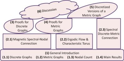
Figure 1.1. Schematic diagram of section dependencies

1.1. Discrete graphs

Let $\mathcal{G}=\left(\mathcal{V},\mathcal{E}\right)$ be a graph with the sets of vertices $\mathcal{V}$ and edges $\mathcal{E}$. All graphs discussed in this paper are connected and have a finite number of vertices and edges. Each edge $e\in\mathcal{E},\,e=\left\{u,v\right\}$ connects a pair of vertices, $u,v\in\mathcal{V}$. We exclude edges which connect a vertex to itself and do not allow two vertices to be connected by more than one edge. For some purposes we would need to consider the directions of the edges. We therefore also define the set $\overleftrightarrow{\mathcal{E}}$ of all graph edges, each appears twice with both its possible directions, and hence $\left|\overleftrightarrow{\mathcal{E}}\right|=2\left|\mathcal{E}\right|$. We use the notation $e=\left(u,v\right)$ to refer to a directed edge $e\in\overleftrightarrow{\mathcal{E}}$ which starts at $u$ and terminates at $v$ and denote the edge with the reversed direction by $\hat{e}:=\left(v,u\right)$. For a vertex $v\in\mathcal{V}$, its degree equals the number of edges connected to it, i.e., $d_{v}:=\left|\left\{u;\,\,\left\{u,v\right\}\in\mathcal{E}\right\}\right|$. Functions on the graph refer to $f:\mathcal{V}\rightarrow\mathbb{R}$ and we now present the operators acting on such functions.

The normalized Laplacian is

(1.1) $$\mathbf{L}_{u,v}^{(norm)}=\begin{cases}-\nicefrac{{1}}{{\sqrt{d_{u}d_{v}}}}&\left(v,u\right)\in\overleftrightarrow{\mathcal{E}}\\ 0&\left(v,u\right)\notin\overleftrightarrow{\mathcal{E}}\\ 1&u=v\end{cases}$$

The normalized Laplacian is a special case of the generalized discrete Laplacian also known as the discrete Schrï¿œdinger operator, a real symmetric matrix which obeys

$$\mathbf{L}_{u,v}<0 \textrm{if }\left\{v,u\right\}\in\mathcal{E}$$

(1.2) $$\mathbf{L}_{u,v}=0 \textrm{if }\left\{v,u\right\}\notin\mathcal{E},$$

and with no constraints on its diagonal values (which are sometimes called in the literature on-site potentials).

These matrices have real eigenvalues which we denote by $\left\{\lambda_{n}\right\}_{n=1}^{\left|\mathcal{V}\right|}$, ordered increasingly, and the corresponding eigenvectors are denoted by $\left\{f_{n}\right\}_{n=1}^{\left|\mathcal{V}\right|}$. The spectrum of the normalized Laplacian belongs to the interval $\left[0,2\right]$. We refer the interested reader to many results concerning the spectra of graph matrices and their eigenvectors which can be found in the books [16, 21, 25] and the references within.

The discrete Schrï¿œdinger operator can be supplied with a magnetic potential, $\mathcal{A}$, which is defined as $\mathcal{A}:\overleftrightarrow{\mathcal{E}}\rightarrow\mathbb{R}$ such that $\mathcal{A}\left(e\right)=-\mathcal{A}\left(\hat{e}\right)$. Assigning such a potential to the operator amounts to the following changes

$$\mathbf{L}\left(\mathcal{A}\right)\ :\ \mathbb{C}^{\left|\mathcal{V}\right|}\rightarrow\mathbb{C}^{\left|\mathcal{V}\right|}$$

$$\mathbf{L}_{u,v}\left(\mathcal{A}\right)=\mathbf{L}_{u,v}\textrm{e}^{i\mathcal{A}\left(u,v\right)},$$

where $\mathbf{L}_{u,v}$ are the entries of the previous (zero magnetic potential) Laplacian. Note that this magnetic operator is still Hermitian and hence has real eigenvalues.

Given a cycle, $\gamma=\left(v_{1},\ldots,v_{n}\right)$, on the graph we define the magnetic flux through this cycle as

$$\alpha_{\gamma}:=\left[\mathcal{A}\left(v_{1},v_{2}\right)+\ldots+\mathcal{A}\left(v_{n-1},v_{n}\right)+\mathcal{A}\left(v_{n},v_{1}\right)\right]\,\textrm{mod}\,2\pi.$$

The graph’s cycles play an important role when introducing magnetic potential. We denote the number of “independent” cycles on the graph as

$$\beta:=\left|\mathcal{E}\right|-\left|\mathcal{V}\right|+1$$

(assuming the graph is connected). This is also known as the first Betti number, which is the dimension of the graph’s first homology. In the following we often fix some arbitrary $\beta$ independent cycles on the graph, $\left\{\gamma_{1},\ldots,\gamma_{\beta}\right\}$ and denote the magnetic fluxes through them by $\left\{\alpha_{1},\ldots,\alpha_{\beta}\right\}$. One can show that given two magnetic potentials, $\mathcal{A}_{1}$ and $\mathcal{A}_{2}$ with the same values for the magnetic fluxes $\left\{\alpha_{i}\right\}_{i=1}^{\beta}$, their corresponding magnetic Laplacians, $\mathbf{L}\left(\mathcal{A}_{1}\right)$ and $\mathbf{L}\left(\mathcal{A}_{2}\right)$ are unitarily equivalent. This unitary equivalence is also known as the gauge invariance principle and means that the spectrum of the Laplacian is uniquely determined by the values $\left\{\alpha_{i}\right\}_{i=1}^{\beta}$ (but not so for its eigenfunctions). We take advantage of this principle, notation-wise, and write the Laplacian and its eigenvalues as functions of the magnetic parameters (fluxes), $\mathbf{L}\left(\vec{\alpha}\right)$ and $\lambda_{n}\left(\vec{\alpha}\right)$, where $\vec{\alpha}:=\left(\alpha_{1},\ldots,\alpha_{\beta}\right)$. Note that in the special case of a tree graph, the gauge invariance principle means that all magnetic Laplacians are unitarily equivalent to the zero magnetic Laplacian, $\mathbf{L}\left(\vec{0}\right)$, and the eigenvalues do not depend on the magnetic potential. More details on magnetic operators on discrete graphs can be found in [22, 47, 56, 60].

1.2. Metric (quantum) graphs

A metric graph is a discrete graph each of whose edges, $e\in\mathcal{E}$, is identified with a one dimensional interval, $[0,l_{e}]$, with a positive finite length $l_{e}$. We use the notation $\vec{l}$ for the vector whose entries are $\left\{l_{e}\right\}_{e\in\mathcal{E}}$. We denote a metric graph by $\Gamma=\left(\mathcal{V},\mathcal{E},\vec{l}\right)$. We can then assign to each edge $e\in\overleftrightarrow{\mathcal{E}}$ a coordinate, $x_{e}$, which measures the distance along the edge from the starting vertex of $e$. In particular, we have the following relation between coordinates of reversed edges, $x_{e}+x_{\hat{e}}=l_{e}$. We denote a coordinate by $x$, when its precise nature is unimportant. A function on the graph is described by its restrictions to the edges, $\left\{\left.f\right|_{e}\right\}_{e\in\overleftrightarrow{\mathcal{E}}}$, where $\left.f\right|_{e}:\left[0,l_{e}\right]\rightarrow\mathbb{C}$ and we require $\left.f\right|_{e}(x_{e})=\left.f\right|_{\hat{e}}(l_{e}-x_{e})$, for all $e\in\overleftrightarrow{\mathcal{E}}$. Therefore, in effect, there is only a single function assigned to each pair of edges, $e,\hat{e}$.

We equip the metric graphs with a self-adjoint differential operator $\mathcal{H}$, the Hamiltonian or metric Schrï¿œdinger operator,

(1.3) $$\mathcal{H}\left(\mathcal{A}\right)\ :\ \left.f\right|_{e}(x_{e})\mapsto\left(\mathbf{\textrm{i}}\frac{\mathbf{\textrm{d}}}{\mathbf{\textrm{d}}x_{e}}+\mathcal{A}_{e}\left(x_{e}\right)\right)^{2}\left.f\right|_{e}\left(x_{e}\right)+V_{e}(x_{e})\left.f\right|_{e}\left(x_{e}\right),$$

where $V_{e}(x)$ is a real valued bounded and piecewise continuous function which forms the electric potential, and $\mathcal{A}_{e}\in C^{1}\left(\left[0,l_{e}\right]\right)$ is called the magnetic potential and it obeys $\mathcal{A}_{e}\left(x_{e}\right)=-\mathcal{A}_{\hat{e}}\left(x_{\hat{e}}\right)$. It is most common to call this setting of a metric graph with a Schrï¿œdinger operator, a quantum graph. We will keep calling these graphs metric graphs to distinguish them from their discrete counterpart which we also equip here with an operator of a quantum nature.

To complete the definition of the operator we need to specify its domain. We denote by $H^{2}(\Gamma)$ the following direct sum of Sobolev spaces

(1.4) $$H^{2}(\Gamma):=\bigoplus_{e\in\overleftrightarrow{\mathcal{E}}}H^{2}([0,l_{e}])\ .$$

The graph’s connectivity is expressed by matching the values of the functions at the common vertices, thus dictating the operator’s domain. All matching conditions that lead to the operator (1.3) being self-adjoint have been classified in [37, 42, 45]. It can be shown that under these conditions the spectrum of $\mathcal{H}$ is real and bounded from below [45]. In addition, since we only consider compact graphs, the spectrum is discrete and with no accumulation points. We number the eigenvalues in the ascending order and denote them (similarly to the discrete case) with $\left\{\lambda_{n}\right\}_{n=1}^{\infty}$ and their corresponding eigenfunctions with $\left\{f_{n}\right\}_{n=1}^{\infty}$. We also use $k_{n}$, such that $\lambda_{n}=k_{n}^{2}$, and say that $\left\{k_{n}\right\}_{n=1}^{\infty}$ is the $k$-spectrum of the graph.

As we wish to study the sign changes of the eigenfunctions, we would require their continuity. The only matching conditions which assure a self-adjoint operator and guarantee that the function is continuous (at the vertices) are the so-called extended $\delta$-type conditions at all the graph’s vertices.

A function $f\in H^{2}(\Gamma)$ is said to satisfy the extended $\delta$-type conditions at a vertex $v$ if

1. $f$ is continuous at $v\in\mathcal{V}$, i.e.,

   $$\forall e_{1},e_{2}\in\overleftrightarrow{\mathcal{E}}_{v\,\,\,\,\,}\left.f\right|_{e_{1}}(0)=\left.f\right|_{e_{2}}(0),$$

   where $\overleftrightarrow{\mathcal{E}}_{v}$ is the set of edges starting at $v$ (so that $x_{e}=0$ at $v$ if $e\in\overleftrightarrow{\mathcal{E}}_{v}$).

2. the outgoing derivatives of $f$ at $v$ satisfy

   (1.5) $$\sum_{e\in\overleftrightarrow{\mathcal{E}}_{v}}\left(\frac{\mathbf{\textrm{d}}}{\mathbf{\textrm{d}}x_{e}}-\mathbf{\textrm{i}}\mathcal{A}_{e}(0)\right)\left.f\right|_{e}\left(0\right)=\chi_{v}f(0),\quad\chi_{v}\in\mathbb{R},$$

   where $f(0)$ denotes the value of $f$ at the vertex (which is uniquely defined due to the first part of the condition).

In particular, the case $\chi_{v}=0$ is often referred to as Neumann condition (also called Kirchhoff or standard condition). We will call a graph whose vertex conditions are all of Neumann type and whose magnetic and electric potentials vanish everywhere, a Neumann graph and state our main results for such graphs. A Neumann graph has $\lambda_{1}=0$ with multiplicity which equals the number of graph’s components (which is always one throughout this paper) and their $k$-spectrum is therefore real and positive. Another useful vertex condition is $\forall e\in\overleftrightarrow{\mathcal{E}}_{v},\,\,\left.f\right|_{e}\left(0\right)=0$. This is called a Dirichlet condition at the vertex $v$, and can be formally written as (1.5) with $\chi_{v}=\infty$. Note that whenever a vertex exhibits a Dirichlet condition, it effectively disconnects all edges connected to this vertex. Similarly to the Neumann graph, a Dirichlet graph is obtained whenever all vertices are supplied with Dirichlet conditions. The eigenvalues of such a graph are merely a union of spectra of its disjoint edges (with Dirichlet conditions at their endpoints) and are called Dirichlet eigenvalues.

An important observation which plays a role in this paper is that the spectrum and eigenfunctions of the graph are not affected if a graph’s edge is divided into two parts by introducing a new vertex (of degree two) at an arbitrary point on this edge and supplying it with Neumann conditions. We call the process (and outcome) of introduction of any number of such vertices on the graph, graph’s subdivision and keep in mind that the spectral properties are invariant with respect to subdivision. Similarly to the definition of discrete graphs, we also exclude edges which connect a vertex to itself and vertices which are connected by more than two edges (reversed to each other). Note, however, that this does not restrict the generality of our results as any metric graph which does have self cycles or multiple edge can be subdivided to eliminate these defects.

The magnetic flux through a cycle, $\gamma=\left(v_{1},\ldots,v_{n}\right)$, is defined as

$$\alpha_{\gamma}:=\sum_{e\in\gamma}\int_{0}^{l_{e}}\mathcal{A}_{e}\,\textrm{d}x_{e},$$

where the notation $e\in\gamma$ means that either $e=\left(v_{i},v_{i+1}\right)$ for some $i$ or $e=\left(v_{n},v_{1}\right)$. The gauge invariance principle introduced previously applies to the metric Schrï¿œdinger operator as well and allows us to write $\mathcal{H}\left(\vec{\alpha}\right)$ and $\lambda_{n}\left(\vec{\alpha}\right)$, when referring to the operator and its eigenvalues. This obviously holds once some fixed choice $\beta$ cycles is made, and the notation $\left\{\alpha_{i}\right\}_{i=1}^{\beta}$ is adapted to fluxes through these cycles, where $\vec{\alpha}:=\left(\alpha_{1},\ldots,\alpha_{\beta}\right)$. Two good references for further reading on the general theory of metric (quantum) graphs are [12, 34].

1.3. The nodal count

The main focus of this paper is the number of sign changes of eigenfunctions on discrete and metric graphs. When counting sign changes we always consider eigenfunctions of the zero magnetic potential operators, as otherwise we are not guaranteed to have real valued eigenfunctions. In addition, in order for the number of sign changes to be well defined we assume the following.

Assumption 1.

The eigenvalue $\lambda_{n}$ is simple and the corresponding eigenfunction, $f_{n}$ is different than zero on every vertex.

We call $\lambda_{n}$ a generic eigenvalue if it satisfies assumption 1 (correspondingly, $f_{n}$ is called a generic eigenfunction). This assumption is generic with respect to various perturbations to the operator. In the discrete case such perturbations include changing the non-zero entries of the matrix $\mathbf{L}$. For a metric graph, one may perturb either the vertex conditions, the edge lengths or the electric potential. Further discussions can be found in [4, 10, 31], where this assumption was used.

We now define sign changes (also known as nodal points) and nodal domains and use the same notations for both metric and discrete graphs.

Definition 1.

1. Let $f_{n}\in H^{2}(\Gamma)$ be generic and the $n^{\textrm{th}}$ eigenfunction of the Schrï¿œdinger operator on a metric graph. The zeros of $f_{n}$ form isolated points on the graph and they correspond to the function’s sign changes. Their set is denoted by $\Phi_{n}$.

2. Let $f_{n}\in\mathbb{R}^{\mathcal{V}}$ be generic and the $n^{\textrm{th}}$ eigenfunction of the discrete Schrï¿œdinger operator on a graph. We say that an edge $e=\left\{u,v\right\}$ forms a sign change (also nodal point) of the eigenfunction if $f_{n}\left(u\right)f_{n}\left(v\right)<0$. The set of these edges is denoted by

   $$\Phi_{n}:=\left\{\left\{u,v\right\}\in\mathcal{E}\,|\,\,f_{n}\left(u\right)f_{n}\left(v\right)<0\right\}.$$

3. The number of nodal points of $f_{n}$ (for both metric and discrete graphs) is called the sign change count or nodal point count of $f_{n}$ and is denoted by $\phi_{n}:=\left|\Phi_{n}\right|$.

4. $\Gamma\backslash\Phi_{n}$ ($\mathcal{G}\backslash\Phi_{n}$) consists of a few subgraphs disconnected one from the other. These subgraphs are called the nodal domains of $f_{n}$ and their number, the nodal domain count, is denoted by $\nu_{n}$.

We also use the general term nodal count, when it is either clear or unimportant whether we count nodal points or nodal domains. We remark that if assumption 1 is not satisfied due to zeros on vertices, the definitions above should be modified. There are indeed alternative definitions of the nodal count in such scenarios (see [6]), but their treatment is out of the scope of this paper.

The known bounds on the nodal count are

(1.6) $$n-1 \leq\phi_{n}\leq n-1+\beta$$

(1.7) $$n-\beta \leq\nu_{n}\leq n.$$

In particular, for a tree graph where $\beta=0$, one obtains $\forall n\,\,\phi_{n}=n-1$. This result for the interval is the famous Sturm’s oscillation theorem [58, 59] and its generalization for trees was done in [52, 55]. The fact that discrete tree graphs also have this nodal count is proven in [11, 28, 29]. The upper bound of (1.7) (Courant bound) is proven in [26] for discrete graphs and in [32] for metric graphs. For both metric and discrete graphs, the upper bound of (1.7) also proves the upper bound of (1.6) since $\phi_{n}\leq\nu_{n}-1+\beta$. The lower bound of (1.7) for both metric and discrete graphs is proven in [11] and the same proof works to prove the lower bound in (1.6) (again for both kinds of graphs).

Two recent works which go further than the above bounds (and from which the bounds (1.6), (1.7) can be deduced) characterize the nodal count of an eigenfunction in terms of a Morse index of a predefined energy function, [4, 14]. These works led to a characterization of the nodal count in terms of Morse indices of magnetic perturbations. This last result is an important tool used in the proofs of the current paper and is described in section 2.1.

1.4. The main results of the current paper

We start by introducing the notation

$$\mathcal{N}:=\left\{n;\,\,\lambda_{n}\,\textrm{satisfies assumption }\ref{ass:generality_assumption}\right\}.$$

Namely, $\lambda_{n}$ is a generic eigenvalue if $n\in\mathcal{N}$.

The two main theorems of this paper are

Theorem 2.

Let $\mathcal{G}$ be a graph supplied with discrete Schrï¿œdinger operator, all of whose eigenvalues are generic, i.e., $\mathcal{N}=\left\{1,\ldots,\left|\mathcal{V}\right|\right\}$. If its nodal point count is such that for all $n\in\mathcal{N}$, $\phi_{n}=n-1$ then $\mathcal{G}$ is a tree graph.

Theorem 3.

Let $\Gamma$ be a Neumann metric graph with at least one generic eigenvalue greater than zero. Then $\Gamma$ has infinitely many generic eigenvalues and exactly one of the following holds

1. $\Gamma$ is a tree and for all $n\in\mathcal{N},\,\phi_{n}=n-1$ and $\nu_{n}=n$.

2. $\Gamma$ is not a tree and each of the sets $\left\{n\in\mathcal{N}\,;\,\phi_{n}>n-1\right\}$, $\left\{n\in\mathcal{N}\,;\,\nu_{n}<n\right\}$ is infinite.

These theorems solve the nodal inverse problem for a tree graph. It is interesting to compare the assumptions and the conclusions of the discrete case with the metric one. The metric theorem shows that a generic nodal count cannot be almost like this of a tree - either it equals a tree’s nodal count or it differs from it for an infinite subsequence. In addition, it allows to conclude that the graph is a tree even if non-generic eigenvalues exist (by simply ignoring them) as long as there is at least one positive generic eigenvalue. The discrete theorem seems to assume more than the metric one, as it requires that all the eigenvalues are generic and all of them have the nodal count of a tree ($\phi_{n}=n-1$). Indeed, in the discrete case, ignoring non-generic eigenvalues is not possible - the normalized Laplacian on the triangle graph, for example, has a single generic eigenfunction with the tree nodal count and two others which are non-generic. The metric theorem also allows to conclude that the graph is a tree based on its nodal domain count. There is, however, no analogous result for discrete graphs. As the final comparison point we mention that the metric theorem solves the inverse problem only for the Laplacian (as it is a Neumann graph and there is no potential) whereas the discrete one applies to the more general Schrï¿œdinger operator.

2. Introducing Tools Needed for the Proofs

2.1. The magnetic spectral-nodal connection

This subsection is devoted to an important connection between the nodal count and the stability of eigenvalues under magnetic perturbation. Such a connection first appeared in [10], where Berkolaiko proved it for discrete graphs. Shortly afterward, the same theorem was reproved by Colin de Verdière who had also shown that the theorem holds for the Hill operator - the metric Schrï¿œdinger operator on a single loop graph, [27]. The proof of the theorem for a general metric graph, due to Berkolaiko and Weyand, appears in another manuscript of this same issue, [15].

Before stating the relevant theorem, we need to introduce the following notations.

1. The difference of the nodal count from its lower bound (also its value in the tree case) is denoted

   $$\sigma_{n}:=\phi_{n}-\left(n-1\right).$$

   Hence, we call it the nodal surplus following [10] (it was also called nodal defect in [27]).

2. The Hessian of the eigenvalue $\lambda$ with respect to magnetic parameters at the point $\vec{\alpha}=\vec{0}$ is denoted by

   $$\left[\mathscr{H}_{\lambda}\left(\vec{0}\right)\right]_{i,j}:=\left.\frac{\partial^{2}\lambda}{\partial\alpha_{i}\partial\alpha_{j}}\right|_{\vec{\alpha}=\vec{0}}.$$

   When $\vec{\alpha}=\vec{0}$ is a critical point of $\lambda\left(\vec{\alpha}\right)$, the Morse index is defined as the number of negative eigenvalues of $\mathscr{H}_{\lambda}\left(\vec{0}\right)$ and it is denoted by $\mathbf{\mathscr{M}}_{\lambda}\left(\vec{0}\right)$.

We collect below the main results of the papers [10, 15, 27] into a single theorem which is applicable for both metric and discrete graphs.

Theorem 4.

[10, 15, 27] Let $\mathcal{G}$ $\left(\Gamma\right)$ be a discrete (metric) graph supplied with a discrete (metric) Schrï¿œdinger operator. Let $\lambda_{n}\left(\vec{\alpha}\right)$ and $f_{n}\left(\vec{\alpha}\right)$ be an eigenvalue and a corresponding eigenfunction of the magnetic operator such that $\lambda_{n}\left(\vec{0}\right)$ and $f_{n}\left(\vec{0}\right)$ satisfy assumption 1. Then the following holds.

1. The point $\vec{\alpha}=\vec{0}$ is a critical point of the function $\lambda_{n}\left(\vec{\alpha}\right)$.

2. The critical point $\vec{\alpha}=\vec{0}$ is non-degenerate.

3. The nodal surplus, $\sigma_{n}$, of the eigenfunction $f_{n}\left(\vec{0}\right)$ is equal to the Morse index of this critical point,

   $$\sigma_{n}=\mathbf{\mathscr{M}}_{\lambda_{n}}\left(\vec{0}\right).$$

2.2. Ergodic flow on the characteristic torus

It is well known that eigenvalues of a metric graph are given, with their multiplicities, as the zeros of a secular function [43, 44],

$$\left\{k^{2};\,\,\tilde{F}\left(k;\,\vec{l};\,\vec{\alpha}\right)=0\right\},$$

where

(2.1) $$\tilde{F}\left(k;\,\vec{l};\,\vec{\alpha}\right):=\det\left(\mathbf{\textrm{e}}^{-\nicefrac{{\mathbf{\textrm{i}}}}{{2}}\left(\mathbf{\mathbf{A}}\left(\vec{\alpha}\right)+k\mathbf{\mathbf{E}}\left(\vec{l}\right)\right)}\right)\det\left(\mathbf{S}\left(k\right)\right)^{-\nicefrac{{1}}{{2}}}\det\left(\mathbf{1}-\mathbf{\textrm{e}}^{\mathbf{\textrm{i}}\left(\mathbf{\mathbf{A}}\left(\vec{\alpha}\right)+k\mathbf{\mathbf{E}}\left(\vec{l}\right)\right)}\mathbf{S}\left(k\right)\right),$$

and $\mathbf{A},\,\mathbf{E}\,\textrm{\,\ and }\mathbf{S}$ are square matrices of dimension $\left|\overleftrightarrow{\mathcal{E}}\right|$ and contain the information about the magnetic fluxes, edge lengths and edge connectivity, respectively. Exact details on the structure of those matrices appear in [34, 44], and we just state here the necessary facts which we use later on:

1. $\mathbf{E}$ is a diagonal matrix of the form

   $$\mathbf{E}=\textrm{diag}\left\{l_{e}\right\}_{e\in\overleftrightarrow{\mathcal{E}}}.$$

2. For a Neumann graph $\mathbf{S}$ is a constant unitary matrix which does not depend on $k$.

3. $\mathbf{A}$ is a diagonal matrix which is linear in $\vec{\alpha}$.

4. $\tilde{F}$ is a real valued function.

Let $\Gamma=\left(\mathcal{V},\mathcal{E},\vec{l}\right)$ be a metric graph. We write its edge lengths as the following linear combinations.

(2.2) $$\forall e\in\mathcal{E}\,\,\,l_{e}=\sum_{i\in I}r_{i}^{\left(e\right)}\xi_{i},$$

where all $r_{i}^{\left(e\right)}$ are rational numbers and $\left\{\xi_{i}\right\}_{i\in I}$ is a set of incommensurate real numbers, i.e., they are linearly independent over the rationals. For example, if all edge lengths are incommensurate then $\left|I\right|=\left|\mathcal{E}\right|$ and the set $\left\{\xi_{i}\right\}_{i\in I}$ can be chosen to consist of the edge lengths. On the other extreme, if all ratios of edge lengths are rational, then $\left|I\right|=1$ and one can choose $\xi_{1}$ to equal any of the edge lengths (or any rational multiple of it). The relations between the edge lengths of the graph, $\left\{l_{e}\right\}_{e\in\mathcal{E}}$, and the parameters $\left\{\xi_{i}\right\}_{i\in I}$ will play an important role later on and we thus define the length map as

$$\mathscr{L}:\mathbb{R}^{I}\rightarrow\mathbb{R}^{\mathcal{E}}$$

(2.3) $$\left[\mathscr{L}\left(\vec{x}\right)\right]_{e}=\sum_{i\in I}r_{i}^{\left(e\right)}x_{i}.$$

This map depends on the specific edge lengths of $\Gamma$ (even the dimension of its domain depends on that) and on the specific choice of values for $\left\{\xi_{i}\right\}_{i\in I}$.

We now describe a method introduced by Barra and Gaspard [9] who related the graph eigenvalues to the Poincaré return times of a flow to a surface defined by the zero level set of the secular function (2.1). We present their method using our length map and start by redefining the secular function

(2.4) $$F\,:\,\mathbb{R}^{I}\times\mathbb{R}^{\beta} \rightarrow \mathbb{R}$$

(2.5) $$F\left(\vec{x};\,\vec{\alpha}\right) := \tilde{F}\left(1;\,\mathscr{L}\left(\vec{x}\right);\,\vec{\alpha}\right).$$

We point out some properties of $F$, which can be deduced from (2.1).

1. $F$ is differentiable.

2. $F\left(k\vec{\xi};\,\vec{\alpha}\right)=\tilde{F}\left(k;\,\mathscr{L}\left(\vec{\xi}\right);\,\vec{\alpha}\right)$ since $\mathscr{L}$ is homogeneous and $\tilde{F}$ contains the parameter $k$ only in the product $k\vec{l}=k\mathscr{L}\left(\vec{\xi}\right)$.

3. $F\left(\vec{x};\,\vec{\alpha}\right)$ is periodic in each of the entries of $\vec{x}$. The period depends on the specific entry, $x_{i}$, and is some rational multiple of $2\pi$.

The last property allows us to (re)define the function $F\left(\cdot;\,\vec{\alpha}\right)$ on an $\left|I\right|$-dimensional torus, $\mathbb{T}^{\left|I\right|}$, with sides depending on the periodicity of $F$ with respect to its parameters, $\left\{x_{i}\right\}_{i\in I}$. Namely,

$$F\,:\,\mathbb{T}^{\left|I\right|}\times\mathbb{R}^{\beta}\rightarrow\mathbb{R},$$

and from now on whenever $F$ is mentioned, its $\vec{x}$ variable is taken modulus this torus periodicity, even if this is not explicitly written. Property (2) allows us to characterize the graph $k$-eigenvalues as

$$\left\{k\left(\vec{\alpha}\right);\,\,F\left(k\vec{\xi};\,\vec{\alpha}\right)=0\right\},$$

where $\vec{\xi}=\mathscr{L}^{-1}\left(\vec{l}\right)$ is the vector with incommensurate entries chosen above. We therefore may define the following flow on the torus

(2.6) $$\vec{x}\left(k\right):=k\vec{\xi},$$

and the surface

(2.7) $$\Sigma_{\vec{\alpha}}:=\left\{F\left(k\vec{\xi};\,\vec{\alpha}\right)=0\right\},$$

so that the $k$-spectrum equals the times (i.e., the $k$ values) for which the flow $\vec{x}\left(k\right)$ pierces $\Sigma_{\vec{\alpha}}$.

Remark 5.

The eigenfunctions which correspond to the graph eigenvalues depend both on the point on the torus, $k\vec{\xi}\in\mathbb{T}^{\left|I\right|}$, and on the specific values of $k$ and $\vec{l}$. The restriction of the eigenfunction to the graph vertices, however, is a continuous function solely of $k\vec{\xi}\in\mathbb{T}^{\left|I\right|}$ (see e.g., [43, 44]). This last observation is exploited in sections 4 and 5.

We end by noting that as the entries of $\vec{\xi}$ are linearly independent over $\mathbb{Q}$, the flow (2.6) is ergodic on $\mathbb{T}^{\left|I\right|}$. This ergodicity is the reason for making the reduction from the set of edge lengths, $\left\{l_{e}\right\}_{e\in\mathcal{E}}$, to $\left\{\xi_{i}\right\}_{i\in I}$. We could have defined the flow on an $\left|\mathcal{E}\right|$-dimensional torus, but then the flow would not necessarily fill the whole torus - it would actually fill a linear subspace given by $\mathscr{L}\left(\mathbb{T}^{\left|I\right|}\right)$ (modulo the $\left|\mathcal{E}\right|$-dimensional torus).

2.3. The spectral connection between metric and discrete graphs

An interesting connection exists between the spectrum of an equilateral metric graph, a graph whose all edge lengths are equal, and the spectrum of the discrete graph which shares the same connectivity. This connection is usually stated in terms of the spectrum of the transition matrix,

(2.8) $$\mathbf{P}_{u,v}=\begin{cases}\nicefrac{{1}}{{d_{u}}}&\left(v,u\right)\in\overleftrightarrow{\mathcal{E}}\\ 0&\left(v,u\right)\notin\overleftrightarrow{\mathcal{E}}\end{cases}.$$

The transition matrix is sometimes referred to as the difference operator or even the discrete Laplace operator, but we will not use it here to avoid confusion. One should note that the transition matrix is not symmetric (and thus does not fall under the definition of the generalized Laplacian), but it is closely related to the normalized Laplacian since

(2.9) $$\mathbf{P}=\mathbf{1}-\mathbf{D}^{\nicefrac{{1}}{{2}}}\mathbf{L}^{\left(norm\right)}\mathbf{D}^{-\nicefrac{{1}}{{2}}},$$

where $\mathbf{D}=\textrm{diag}\left\{d_{v}\right\}_{v\in\mathcal{V}}$ is a diagonal matrix which contains all vertex degrees. If $\lambda,f$ are an eigenvalue and an eigenvector of $\mathbf{L}^{\left(norm\right)}$, then $\mathbf{P}$ has $1-\lambda$ and $\mathbf{D}^{\nicefrac{{1}}{{2}}}f$ as its corresponding eigenpair. We use this connection between both operators to slightly rephrase a known result which usually refers to the spectrum of the transition matrix.

Theorem 6.

[20, 45, 50, 62, 63] Let $\mathcal{G}$ be a discrete graph and $\Gamma$ be a metric graph with the same connectivity and such that $\forall e\,\,l_{e}=1$. Consider the normalized Laplacian, $\mathbf{L}^{\left(norm\right)}$, on $\mathcal{G}$ and the metric Laplacian with Neumann conditions on $\Gamma$. Equip both operators with magnetic fluxes for some choice of $\beta$ cycles on the graph (the same choice for both $\mathcal{G}$ and $\Gamma$). Let $\mu\left(\vec{\alpha}\right)\notin\left\{0,2\right\}$ be an eigenvalue of $\mathcal{G}$ and $f\left(\vec{\alpha}\right)$ the corresponding eigenvector. Then

1. All values in the infinite set $\left\{\left(\arccos\left[1-\mu\left(\vec{\alpha}\right)\right]\right)^{2}\right\}$ are eigenvalues of the magnetic metric Schrï¿œdinger operator on $\Gamma$. We consider here $\arccos$ as a multivalued function, $\arccos:\left[-1,1\right]\rightarrow\left[0,\infty\right)$.

2. When $\vec{\alpha}=\vec{0}$, the other eigenvalues of the metric Schrï¿œdinger operator are the Dirichlet eigenvalues, all of which belong to the set $\left\{\left(\pi n\right)^{2}\right\}_{n\in\mathbb{Z}}$.

3. An eigenfunction corresponding to any of the eigenvalues $\left(\arccos\left[1-\mu\left(\vec{\alpha}\right)\right]\right)^{2}$ equals to $\mathbf{D}^{\nicefrac{{1}}{{2}}}f\left(\vec{\alpha}\right)$ when restricted to $\Gamma$’s vertices.

The content of the theorem for the zero magnetic potential case appears in [20, 45, 62, 63], where they mostly treat Neumann vertex conditions (except in [63] where the so called anti-Kirchhoff conditions are treated as well). A more general derivation which includes electric and magnetic potentials as well as $\delta$-type conditions appears in [50]. In most works above the results are stated in terms of the transition matrix, (2.8), but we prefer to relate to the normalized Laplacian as theorem 4 applies to it.

3. Proofs for Discrete Graphs

The next theorem brings one of the two results which inspire this paper’s title. It is stated and proved here for discrete graphs, whereas the metric case appears in the next section.

Proof of theorem 2.

Assume by contradiction that $\mathcal{G}$ is not a tree. Namely $\beta>0$, and we may therefore supply the graph with a magnetic potential and apply theorem 4. From the assumption in our theorem we get for the nodal surplus

$$\forall n\,\,\sigma_{n}=\phi_{n}-\left(n-1\right)=0.$$

We apply theorem 4 for $\lambda_{n}\left(\vec{\alpha}\right)$ - the third part of the theorem allows to conclude that $\lambda_{n}\left(\vec{\alpha}\right)$ has a minimum at $\vec{\alpha}=\vec{0}$ and the second part shows that this minimum is strict. Therefore, the eigenvalue sum, $\sum_{n}\lambda_{n}\left(\vec{\alpha}\right)$, also has a strict minimum at $\vec{\alpha}=\vec{0}$ . However, since the diagonal entries of the Laplacian do not depend on the magnetic parameters, $\vec{\alpha}$, we get that $\textrm{trace}\left\{\mathbf{L}\left(\vec{\alpha}\right)\right\}$ is a constant function of $\vec{\alpha}$. Hence we arrive at a contradiction, due to $\sum_{n}\lambda_{n}\left(\vec{\alpha}\right)=\textrm{trace}\left\{\mathbf{L}\left(\vec{\alpha}\right)\right\}$. ∎

The essence of the proof above is to show that the zero sequence is not a valid candidate as a nodal surplus sequence. This is done by identifying $\textrm{trace}\left\{\mathbf{L}\left(\vec{\alpha}\right)\right\}$ as a spectral invariant independent of the magnetic potential. We wish to point out similar results which are obtained from such a method. An immediate next step would be to observe that $\textrm{trace}\left\{\mathbf{L}^{2}\left(\vec{\alpha}\right)\right\}$ is a constant function of $\vec{\alpha}$ as well. Computing its Hessian and expressing it in terms of the eigenvalues and their Hessians, $\mathscr{H}_{\lambda_{n}}$, gives

(3.1) $$\sum_{n=1}^{\left|\mathcal{V}\right|}\lambda_{n}\left(\vec{0}\right)\mathscr{H}_{\lambda_{n}}\left(\vec{0}\right)=\mathbf{0},$$

where we have used $\forall n\,\forall i\,\,\frac{\partial}{\partial\alpha_{i}}\lambda_{n}\left(\vec{0}\right)=0$, which we get from theorem 4 (part (1)). Similarly, the magnetic invariance of $\textrm{trace}\left\{\mathbf{L}\left(\vec{\alpha}\right)\right\}$ gives

(3.2) $$\sum_{n=1}^{\left|\mathcal{V}\right|}\mathscr{H}_{\lambda_{n}}\left(\vec{0}\right)=\mathbf{0}.$$

Combining (3.2) and (3.1) allows to prove the following.

Proposition 7.

Let $\mathcal{G}$ be a graph with $\beta$ cycles supplied with discrete Schrï¿œdinger operator such that all of its eigenvalues are generic. Its nodal count cannot be of the form

$$\phi_{n}=\begin{cases}n-1&\,\,\,n\leq m\\ n-1+\beta&\,\,\,n>m\end{cases}$$

for any $m$.

Proof.

Assume by contradiction that the graph has the above nodal count. Namely, the graph’s surplus sequence is of the form $\left\{0,\ldots,0,\beta,\ldots,\beta\right\}$. From theorem 4 we get that

(3.3) $$\forall\,\,1\leq n\leq m \mathscr{H}_{\lambda_{n}}\left(\vec{0}\right)>\mathbf{0}$$

(3.4) $$\forall\,\,m+1\leq n\leq\left|\mathcal{V}\right| \mathscr{H}_{\lambda_{n}}\left(\vec{0}\right)<\mathbf{0}$$

where the first (second) inequality above means that the Hessians are positive (negative) definite quadratic forms. Note that $m<\left|\mathcal{V}\right|$ due to theorem 2. We rewrite (3.1) as

$$\mathbf{0} = \sum_{n=1}^{m}\lambda_{n}\left(\vec{0}\right)\mathscr{H}_{\lambda_{n}}\left(\vec{0}\right)+\sum_{n=m+1}^{\left|\mathcal{V}\right|}\lambda_{n}\left(\vec{0}\right)\mathscr{H}_{\lambda_{n}}\left(\vec{0}\right)$$

$$< \lambda_{m+1}\left(\vec{0}\right)\sum_{n=1}^{m}\mathscr{H}_{\lambda_{n}}\left(\vec{0}\right)+\lambda_{m+1}\left(\vec{0}\right)\sum_{n=m+1}^{\left|\mathcal{V}\right|}\mathscr{H}_{\lambda_{n}}\left(\vec{0}\right)$$

$$= \lambda_{m+1}\left(\vec{0}\right)\sum_{n=1}^{\left|\mathcal{V}\right|}\mathscr{H}_{\lambda_{n}}\left(\vec{0}\right),$$

where we used (3.3), (3.4) and the fact that eigenvalues are ordered increasingly to get the second line. The last line is proportional to (3.2), which gives the contradiction. ∎

Carrying on with this route and examining traces of higher powers of the operator, shows that in general $\textrm{trace}\left\{\mathbf{L}^{k}\left(\vec{\alpha}\right)\right\}$ might depend on the magnetic parameters. More specifically, a direct calculation of $\textrm{trace}\left\{\mathbf{L}^{k}\left(\vec{\alpha}\right)\right\}$ shows that it can be expressed as an expansion over closed walks of size $k$ on the graph. Examining the dependence of such walks on magnetic parameters brings about the following.

Theorem 8.

Let $\mathcal{G}$ be a non-tree graph ($\beta>0$) with discrete Schrï¿œdinger operator such that all of its eigenvalues are generic. Then the size of the graph’s shortest cycle (its girth) is

$$\min_{k}\left\{\sum_{n}\lambda_{n}^{k-1}\mathscr{H}_{\lambda_{n}}\neq\mathbf{0}\right\}.$$

Alternatively, it also equals $\min_{k}\left\{\sum_{n}\lambda_{n}^{k-1}\textrm{trace}\mathscr{H}_{\lambda_{n}}\neq 0\right\}$.

Proof.

The Hessian of $\textrm{trace}\left\{\mathbf{L}^{k}\right\}$ is obtained in terms of Hessians of the eigenvalues as

(3.5) $$\mathscr{H}{}_{\textrm{trace}\left\{\mathbf{L}^{k}\right\}}\left(\vec{0}\right)=\sum_{n=1}^{\left|\mathcal{V}\right|}\lambda_{n}^{k-1}\mathscr{H}_{\lambda_{n}}\left(\vec{0}\right),$$

where we used theorem 4 to conclude that $\lambda_{n}$ has a critical point at $\vec{\alpha}=\vec{0}$, and therefore no first derivatives of $\lambda_{n}$ appear above. The diagonal entries of $\mathbf{L}^{k}$ can be expressed using closed walks on the graph. We define a closed walk by $\gamma=\left(v_{0},v_{1},\ldots,v_{k-1}\right)$, where for all $0\leq i\leq k-1$ either $v_{i}=v_{i+1}$ or $\left(v_{i},v_{i+1}\right)\in\overleftrightarrow{\mathcal{E}}$ (we denote $v_{k}:=v_{0}$ and keep in mind that $\gamma$ is defined up to cyclic permutations). This is similar to the usual notion of closed walks, but we allow the walk to stop at any vertex for a (discrete) while before continuing to the next one. The set of all closed walks of size $k$, passing through vertex $v$, is denoted $\mathcal{C}_{v}^{\left(k\right)}$ and we attribute to each walk a weight obtained as a product of all corresponding Laplacian entries,

$$L_{\gamma}:=\mathbf{L}_{v,v_{k-1}}\ldots\mathbf{L}_{v_{2},v_{1}}\mathbf{L}_{v_{1},v},$$

where the notation $v:=v_{0}$ is implied. The expression above depends on the magnetic parameters, which we omit for the sake of brevity. The diagonal entries of $\mathbf{L}^{k}$ can be now written as

$$\left[\mathbf{L}^{k}\right]_{v,v}=\sum_{\gamma\in\mathcal{C}_{v}^{\left(k\right)}}L_{\gamma}.$$

Denote by $\kappa$ the graph’s girth. For $k<\kappa$, the closed walks $\gamma\in\mathcal{C}_{v}^{\left(k\right)}$ do not circulate any cycle and therefore their weights, $L_{\gamma}$, are independent of magnetic parameters (as can also be seen by a direct calculation of $L_{\gamma}$). We thus get from (3.5) that $\min_{k}\left\{\sum_{i}\lambda_{i}^{k-1}\mathscr{H}_{\lambda_{i}}\neq\mathbf{0}\right\}\geq\kappa$ and it is left to show that this is actually an equality. For $k=\kappa$, let $\gamma=\left(v,v_{1},\ldots,v_{k-1}\right)$ be a closed walk on the graph which contains one of the graph’s cycles. The walk $\gamma$ must have all of its vertices different from each other, as $k$ is the length of the shortest cycle on the graph. The contribution to $\left[\mathbf{L}^{k}\right]_{v,v}$ comes only from $\gamma$ and other walks which circulate one of the graph cycles. We may couple all such walks to

$$\gamma=\left(v,v_{1},\ldots,v_{k-1}\right)\,\textrm{and \,\ }\hat{\gamma}=\left(v,v_{k-1},\ldots,v_{1}\right),$$

and get that their contributions are complex conjugates of each other, $L_{\gamma}=\overline{L_{\hat{\gamma}}}$. From $\mathbf{L}\left(\vec{\alpha}\right)$ being Hermitian and $\mathbf{L}\left(\vec{0}\right)$ having negative off-diagonal entries, we get

$$L_{\gamma}+L_{\hat{\gamma}}=\left(-1\right)^{k}\left|L_{\gamma}\right|2\cos\left(\vec{n}\cdot\vec{\alpha}\right),$$

where $\vec{n}\in\mathbb{Z}^{\beta}$. As $\gamma$ circulates one of the graph cycles, $\vec{n}\neq\vec{0}$ and therefore

$$\exists i\,\,\textrm{s.t. \,}\left.\frac{\partial^{2}}{\partial\alpha_{i}^{2}}\left(L_{\gamma}+L_{\hat{\gamma}}\right)\right|_{\vec{\alpha}=\vec{0}}\neq 0.$$

In particular, all such second derivatives which do not vanish have a definite sign, which equals to $\left(-1\right)^{k+1}$. Therefore, summing over all such couples, $\gamma,\hat{\gamma}$ gives

$$\textrm{sign}\left\{\left.\frac{\partial^{2}}{\partial\alpha_{i}^{2}}\left(\left[\mathbf{L}^{k}\right]_{v,v}\right)\right|_{\vec{\alpha}=\vec{0}}\right\}=\left(-1\right)^{k+1},$$

and therefore also

$$\textrm{sign}\left\{\left.\frac{\partial^{2}}{\partial\alpha_{i}^{2}}\left(\textrm{trace}\left\{\mathbf{L}^{k}\right\}\right)\right|_{\vec{\alpha}=\vec{0}}\right\}=\left(-1\right)^{k+1}.$$

This shows that for $k=\kappa$, the trace of the Hessian in (3.5) is different than zero and completes the proof.∎

Remark 9.

Note that the proof would work similarly if the second derivatives are calculated with respect to the magnetic potential on the single edges (rather then the flux over a cycle). In such a case, the theorem can be extended to include tree graphs as well. In addition, these derivatives are more accessible for computation, especially we are only given the Laplacian and the graph’s connectivity is unknown, which is relevant as we are dealing with inverse problems.

Theorem 8 goes a step forward from theorem 2 as it allows to obtain some information on the graph’s cycles. Yet, the information used in this inverse result is purely spectral - eigenvalues and their perturbations with respect to magnetic potentials. It would be interesting to see if one may obtain results of similar character from the nodal count of the graph. A possible direction might be to examine the magnetic derivatives of traces of powers of the Laplacian (as in the proof of theorem 8) or the magnetic derivatives of the coefficients of the characteristic polynomial. Theorem 4 would probably be a main tool in such an exploration. Indeed, in the course of the proof of theorem 8 we did not exploit the full strength of theorem 4 and used it only to claim that all first magnetic derivatives vanish. Applying the spectral-nodal connection which theorem 4 offers to gather information on the graph cycles, might be an important step in developing a trace formula for the nodal count. A further discussion on this direction is found in section 6.

4. Proofs for Metric Graphs

The main result of this paper for metric graphs (theorem 3) follows from the next lemma and theorem.

Lemma 10.

Let $\Gamma$ be a Neumann metric graph with at least one generic eigenvalue greater than zero. Then $\Gamma$ has infinitely many generic eigenvalues.

Theorem 11.

Let $\Gamma$ be a Neumann metric graph with $\beta>0$ cycles and at least one generic eigenvalue greater than zero. Denote by $\sigma$ the nodal surplus of such an eigenvalue. Then

1. there are infinitely many generic eigenvalues whose nodal surplus equals $\sigma$.

2. there are infinitely many generic eigenvalues whose nodal surplus equals $\beta-\sigma$.

We first apply lemma 10 and theorem 11 to prove theorem 3, and then proceed to prove them as well.

Proof of theorem 3.

Observe that $\Gamma$ has infinitely many generic eigenvalues as a direct conclusion of lemma 10. If $\Gamma$ is a tree graph then it was proved in [52, 55] (see also appendix A in [11]) that the nodal counts of all generic eigenfunctions are $\phi_{n}=n-1$ and $\nu_{n}=n$. Otherwise, if $\Gamma$ has $\beta>0$ cycles, assume by contradiction that there are only finitely many generic eigenfunctions with $\phi_{n}\neq n-1$. In particular this means that there is at least one generic eigenfunction for which $\phi_{n}=n-1$ and thus $\sigma_{n}=0$. We may therefore conclude from theorem 11 that there are infinitely many generic eigenfunctions whose surplus is $\beta$ ($\phi_{n}=n-1+\beta$) and get a contradiction.

In order to prove the statement about the nodal domain count we use the following connection between nodal point count and nodal domain count for metric graphs, which is proved for example in [4] (see there, equation (1.11) together with lemma 3.2),

(4.1) $$\exists n_{0}\,\textrm{ s.t. \,}\forall n>n_{0}\,\quad\phi_{n}=\nu_{n}-1+\beta.$$

Now, assume by contradiction that there are only finitely many eigenfunctions with $\nu_{n}<n$. Then there exists some $n_{1}>n_{0}$ such that for all $n\in\mathcal{N}\cap\left(n_{1},\infty\right),\,\nu_{n}=n$ and from (4.1) we get that for all $n\in\mathcal{N}\cap\left(n_{1},\infty\right),\,\phi_{n}=n-1+\beta.$ The surplus of all these eigenfunction is $\beta$. Applying theorem 11 gives that there are also infinitely many generic eigenfunctions with surplus equals to zero, but the conclusion in the previous sentence allows for only finitely many surpluses to differ than $\beta$ and hence the contradiction. ∎

We now proceed to the proof of lemma 10, and bring two additional lemmata, all of which will be used to prove theorem 11. In the following we refer to $k_{n}\left(\vec{\alpha}\right)=\sqrt{\lambda_{n}\left(\vec{\alpha}\right)}$ as the graph eigenvalues, which is valid and done for the sake of simplicity.

Proof of lemma 10.

Let $\vec{\xi}\in\mathbb{R}^{I}$ be a vector of incommensurate entries which express the graph edge lengths by (2.2). Let $k_{0}$ be a generic eigenvalue of $\Gamma$. Note that the graph eigenvalues are given as zeros of $F$ together with their multiplicities (a property that $F$ inherits from $\tilde{F}$, see (2.1) and (2.5)). We therefore get that $\frac{\textrm{d}}{\textrm{d}k}F\neq 0$ at simple eigenvalues. As we assumed $k_{0}$ to be a simple eigenvalue we have $\left.\frac{\textrm{d}}{\textrm{d}k}F\right|_{\left(k_{0}\vec{\xi},\vec{0}\right)}=\left.\vec{\xi}\cdot\vec{\nabla}F\right|_{\left(k_{0}\vec{\xi},\vec{0}\right)}\neq 0$. We know that $k_{0}\vec{\xi}\in\Sigma_{\vec{0}}$, as $k_{0}$ is an eigenvalue and $\Sigma_{\vec{0}}$ is the zero set of $F$ (recall section 2.2). Choose a neighbourhood $\Xi$ of $k_{0}\vec{\xi}$ on $\Sigma_{\vec{0}}$ such that $\left.\vec{\xi}\cdot\vec{\nabla}F\right|_{\left(\vec{x},\vec{0}\right)}\neq 0$ for all $\vec{x}\in\Xi$. Recall (remark 5) that the values the eigenfunction obtains on the graph vertices are a continuous function of $\vec{x}$. From the genericity of $k$ we know that its corresponding eigenfunction does not vanish on the vertices and we may therefore choose $\Xi$ small enough such that this property holds for all $\vec{x}\in\Xi$. As the flow is ergodic, the set $\Xi\subset\Sigma_{\vec{0}}$ will be pierced an infinite number of times by the flow, yielding infinitely many eigenvalues. Our choice of $\Xi$ guarantees both that these eigenvalues are simple and that their corresponding eigenfunctions do not vanish on vertices.∎

Lemma 12.

Let $\vec{\xi}\in\mathbb{R}^{I}$ be a vector of incommensurate entries which express the graph edge lengths by (2.2). Let $k\left(\vec{0}\right)\neq 0$ be a generic eigenvalue. The Hessian of this eigenvalue with respect to the magnetic fluxes at $\vec{\alpha}=\vec{0}$ is given as

(4.2) $$\mathscr{H}_{k}\left(\vec{0}\right)=-\left.\frac{\mathscr{H}_{F}}{\left(\vec{\xi}\cdot\vec{\nabla}F\right)}\right|_{\left(k\left(\vec{0}\right)\vec{\xi};\vec{0}\right)},$$

where $\mathscr{H}_{F}$ denotes the Hessian of the secular function $F\left(k\left(\vec{0}\right)\vec{\xi};\cdot\right)$ with respect to its magnetic parameters and $\vec{\nabla}F$ is the gradient of $F\left(\cdot;\vec{0}\right)$ taken with respect to its coordinates on the torus $\mathbb{T}^{\left|I\right|}$.

Proof.

The eigenvalue $k\left(\vec{\alpha}\right)$ is given implicitly as the solution of $F\left(k\left(\vec{\alpha}\right)\vec{\xi};\,\vec{\alpha}\right)=0$. Take the second total derivatives of this expression with respect to any two magnetic fluxes,

$$0 = \frac{\textrm{d}^{2}}{\textrm{d}\alpha_{i}\textrm{d}\alpha_{j}}F\left(k\left(\vec{\alpha}\right)\vec{\xi};\,\vec{\alpha}\right)$$

$$= \frac{\partial^{2}k}{\partial\alpha_{i}\partial\alpha_{j}}\left(\vec{\xi}\cdot\vec{\nabla}F\right)+\frac{\partial k}{\partial\alpha_{i}}\frac{\partial k}{\partial\alpha_{j}}\sum_{p,q=1}^{\left|I\right|}\frac{\partial^{2}F}{\partial x_{p}\partial x_{q}}\xi_{p}\xi_{q}+\frac{\partial k}{\partial\alpha_{j}}\left(\vec{\xi}\cdot\frac{\partial}{\partial\alpha_{j}}\vec{\nabla}F\right)+\frac{\partial^{2}F}{\partial\alpha_{i}\partial\alpha_{j}}.$$

Evaluate the above at the point $\vec{\alpha}=\vec{0}$ and use $\forall i\,\left.\frac{\partial k}{\partial\alpha_{i}}\right|_{\vec{\alpha}=\vec{0}}=0$ (theorem 4, part (1)), to get that the second and the third terms above vanish and we are left with

(4.3) $$\left.\left\{\left(\vec{\xi}\cdot\vec{\nabla}F\right)\mathscr{H}_{k}\left(\vec{0}\right)+\mathscr{H}_{F}\right\}\right|_{\left(k\left(\vec{0}\right)\vec{\xi},\vec{0}\right)}=0.$$

We now repeat the argument in the proof of lemma 10 to conclude that if $k\left(\vec{0}\right)$ is simple then $\left.\frac{\textrm{d}}{\textrm{d}k}F\right|_{\left(k\left(\vec{0}\right)\vec{\xi},\vec{0}\right)}=\left.\vec{\xi}\cdot\vec{\nabla}F\right|_{\left(k\left(\vec{0}\right)\vec{\xi},\vec{0}\right)}\neq 0$. Thus, we divide (4.3) by $\left.\vec{\xi}\cdot\vec{\nabla}F\right|_{\left(k\left(\vec{0}\right)\vec{\xi},\vec{0}\right)}$ to get (4.2).∎

Lemma 13.

The secular function $F$ of a Neumann graph exhibits the following symmetry

(4.4) $$F\left(\vec{x};\,\vec{\alpha}\right)=F\left(-\vec{x};\,-\vec{\alpha}\right).$$

Proof.

Let $\vec{x}\in\mathbb{T}^{\left|I\right|}$ and $\alpha\in\mathbb{R}^{\beta}$. Choose some $\vec{\xi}\in\mathbb{R}^{\left|I\right|}$ with incommensurate entries. There exists $k\in\mathbb{R}$ such that $\vec{x}\equiv k\vec{\xi}$ modulo $\mathbb{T}^{\left|I\right|}$. The required symmetry (4.4) is now obtained from the following series of equalities.

$$F\left(k\vec{\xi};\,\vec{\alpha}\right)= \tilde{F}\left(k;\,\mathscr{L}\left(\vec{\xi}\right);\,\vec{\alpha}\right) =\overline{\tilde{F}\left(-k;\,\mathscr{L}\left(\vec{\xi}\right);\,-\vec{\alpha}\right)}$$

$$=\tilde{F}\left(-k;\,\mathscr{L}\left(\vec{\xi}\right);\,-\vec{\alpha}\right)=F\left(-k\vec{\xi};\,-\vec{\alpha}\right).$$

The first and last equalities result from property (2), mentioned after the definition of $F$ on the torus, (2.5). The second equality can be deduced from (2.1) together with the linearity of $\mathbf{\mathbf{A}}\left(\vec{\alpha}\right)$ and the observation that $\mathbf{S}\left(k\right)$ is real and $k$-independent for a Neumann graph. Finally, the third inequality (from the first to the second line) is due to $\tilde{F}$ being real. ∎

Proof of theorem 11.

Denote the edge lengths of $\Gamma$ by the vector $\vec{l}$ and choose an incommensurate set $\vec{\xi}\in\mathbb{R}^{I}$ which is related to graph edge lengths by (2.2). Let $k$ be a generic eigenvalue of $\Gamma$ whose nodal surplus is $\sigma$. The Hessian of $k$ is given by (4.2) in lemma 12 and we know from theorem 4 part (2) that it is non-degenerate. We may therefore choose a neighbourhood $\Xi$ of $k\vec{\xi}$ on $\Sigma_{\vec{0}}$ such that $\left.\frac{\mathscr{H}_{F}}{\left(\vec{\xi}\cdot\vec{\nabla}F\right)}\right|_{\left(\vec{x},\vec{0}\right)}$ is non-degenerate for all $\vec{x}\in\Xi$, and thus the number of negative eigenvalues of $\left.\frac{\mathscr{H}_{F}}{\left(\vec{\xi}\cdot\vec{\nabla}F\right)}\right|_{\left(\vec{x},\vec{0}\right)}$ stays constant in this neighbourhood. This number equals to the Morse index of the eigenvalue and it equals to $\sigma$ by an application of theorem 4 (part (3)). As the flow is ergodic, the set $\Xi\subset\Sigma_{\vec{0}}$ is pierced an infinite number of times by the flow, yielding infinitely many eigenvalues. All of these eigenvalues are generic if $\Xi$ is chosen small enough, as can be shown by repeating the argument in the proof of lemma 10. Each of these eigenvalues would have this same Morse index, $\sigma$, by (4.2). The nodal surplus of each of these eigenvalues is therefore also equal to $\sigma$, according to theorem 4 (part (3)) and this proves the first statement in our theorem. The second statement is proved with the aid of the symmetry (4.4) in lemma 13, which allows to conclude

$$\forall\vec{x}\in\Xi\,\,\,\,;\left.\mathscr{H}_{F}\right|_{\left(\vec{x},\vec{0}\right)} = \left.\mathscr{H}_{F}\right|_{\left(-\vec{x},\vec{0}\right)}$$

$$\left.\vec{\nabla}F\right|_{\left(\vec{x},\vec{0}\right)} = -\left.\vec{\nabla}F\right|_{\left(-\vec{x},\vec{0}\right)},$$

from which we get

(4.5) $$\forall\vec{x}\in\Xi\,\,\,\,;-\left.\frac{\mathscr{H}_{F}}{\left(\vec{\xi}\cdot\vec{\nabla}F\right)}\right|_{\left(\vec{x},\vec{0}\right)} = \left.\frac{\mathscr{H}_{F}}{\left(\vec{\xi}\cdot\vec{\nabla}F\right)}\right|_{\left(-\vec{x},\vec{0}\right)}.$$

The LHS has $\sigma$ negative eigenvalues and therefore the RHS has $\beta-\sigma$ negative eigenvalues. From (4.4) we also deduce $\Xi\subset\Sigma_{\vec{0}}\,\Rightarrow\,-\Xi\subset\Sigma_{\vec{0}}$ (where $-\Xi:=\left\{\vec{x};\,\,-\vec{x}\in\Xi\right\}$). Now use again the ergodicity of the flow to conclude that the set $-\Xi$ is pierced an infinite number of times by the flow and all resulting eigenvalues have Morse index $\beta-\sigma$, which equals to their nodal surplus following theorem 4.∎

Remark 14.

The proof above essentially enables the proof of the metric inverse nodal theorem (theorem 3). One might note that the proof here is of a different nature than the proof of the discrete inverse nodal theorem (theorem 2), where we have identified the trace of the operator as a spectral invariant independent of magnetic potential. One can find, however, a similarity between the proofs, as the antisymmetric relation (4.5) points on the possibility to average the Hessians over whole torus and show that the magnetic dependence cancels.

Remark 15.

In the course of the proof we have used an equality between the Morse index of a particular eigenvalue and the Morse index of the secular function $F$ evaluated at the appropriate point. A similar relation appears in appendix E of [27] where the Morse index of an eigenvalue is expressed in terms of the Morse index of the characteristic polynomial evaluated at this eigenvalue.

Remark 16.

The symmetry which lemma 13 describes can already be exhibited on the level of the Schrï¿œdinger operator on the graph. One can show that the $\vec{\alpha}\rightleftarrows-\vec{\alpha}$ symmetry amounts to conjugation of all the eigenvalues (see (1.3)), which actually leaves the spectrum invariant as it is real. Lemma 13 tells us that the transformation $\vec{\alpha}\rightarrow-\vec{\alpha}$ changes the sign of the $k$-eigenvalues, which also leaves the spectrum invariant. This spectral symmetry was exploited in [15, 27] to prove that the eigenvalues have critical points at $\vec{\alpha}=\vec{0}$.

5. Discretized Versions of a Metric Graph

This section presents a connection between a certain metric graph and various discrete graphs with similar nodal surplus. These discrete graphs can be obtained from the metric one by means of a simple construction and they will be called its discretized versions. This correspondence between a metric graph and its discretized versions is interesting on its own and can also be used as a tool to provide an additional proof for theorem 11 and thus also for the inverse result in theorem 3. More interestingly, this might be used to further extend theorem 3 for graphs with general vertex conditions and electric potentials (see remark 20).

The construction starts by picking a vector $\vec{\xi}\in\mathbb{R}^{I}$ of incommensurate entries such that the graph edge lengths are given by $\vec{l}=\mathscr{L}\left(\vec{\xi}\right)$ (as in section 2.2). The specific discretized version we construct is characterized by a selection of

(5.1) $$\vec{j}\in\textrm{Image}\left(\mathscr{L}\right)\cap\mathbb{N}^{\mathcal{E}}.$$

Note that the set $\textrm{Image}\left(\mathscr{L}\right)\cap\mathbb{N}^{\mathcal{E}}$ is non-empty. In order to show this, one can approximate $\vec{\xi}$ by some rational vector, $\vec{\xi}^{rat}\in\mathbb{Q}^{I}$, such that $\mathscr{L}\left(\vec{\xi}^{rat}\right)$ has all positive entries (just as $\vec{l}=\mathscr{L}\left(\vec{\xi}\right)$ does). Note that $\mathscr{L}\left(\vec{\xi}^{rat}\right)\in\mathbb{Q}^{\mathcal{E}}$ (see (2.2)), and therefore the vector $\mathscr{L}\left(\vec{\xi}^{rat}\right)$ can now be multiplied by a common divisor of its entries to turn its entries to natural numbers, while retaining it in $\textrm{Image}\left(\mathscr{L}\right)$.

Take the underlying discrete graph of the metric graph, $\Gamma$, and equip each edge $e\in\mathcal{E}$ with $j_{e}-1$ new vertices of degree two, which will split this edge into $j_{e}$ new edges. This (new) discrete graph is denoted $\mathcal{G}_{\Gamma}$ and called a discretized version of $\Gamma$. Note that a discretized version is not uniquely determined by $\Gamma$. The set of all possible discretized versions is given by $\textrm{Image}\left(\mathscr{L}\right)\cap\mathbb{N}^{\mathcal{E}}$. This set depends on the ’nature of incommensurability’ of the original edge lengths, $\left\{l_{e}\right\}_{e\in\mathcal{E}}$, i.e., the rational dependencies between these lengths. However, one can verify that $\textrm{Image}\left(\mathscr{L}\right)\cap\mathbb{N}^{\mathcal{E}}$ does not depend on the particular choice of incommensurate representatives, $\left\{\xi_{i}\right\}_{i\in I}$.

Note that one may convert the discretized graph, $\mathcal{G}_{\Gamma}$, back into a metric graph (different than $\Gamma$) by setting all of $\mathcal{G}_{\Gamma}$’s edge lengths to equal one. One would then get a metric graph with the same connectivity as $\Gamma$, but with integer edge lengths given by $\vec{j}$. We denote this metric graph by $\tilde{\Gamma}$ and it will turn to be useful in the course of proving the following.

Theorem 17.

Let $\Gamma$ be a Neumann metric graph with $\beta>0$ cycles and let $\mathcal{G}_{\Gamma}$ be a discretized version of $\Gamma$. Let $\mu\notin\left\{0,2\right\}$ be a generic eigenvalue of $\mathbf{L}^{\left(norm\right)}$ on $\mathcal{G}_{\Gamma}$ whose nodal surplus is $\sigma$. Then

1. $\Gamma$ has infinitely many generic eigenvalues whose nodal surplus equals $\sigma$.

2. $\Gamma$ has infinitely many generic eigenvalues whose nodal surplus equals $\beta-\sigma$.

Remark 18.

It is important to emphasize that the theorem holds for all discretized versions, $\mathcal{G}_{\Gamma}$, of a metric graph, $\Gamma$.

Remark 19.

One should note that the theorem is empty if the spectrum of the chosen discretized version consists only of the eigenvalues $\left\{0,2\right\}$ and other non-generic eigenvalues. The only connected graph which has no eigenvalues different from $\left\{0,2\right\}$ is the single edge graph (see for example, lemma 1.8 in [21]). Nevertheless it does not fit our theorem as it has no cycles. Yet, there are discrete graphs (with cycles) whose all eigenvalues which are different than $\left\{0,2\right\}$ are not simple. The $n-$cube graph forms such an example (example 1.6 in [21]). Following the previous remark, one may still wonder whether for given a metric graph, there is always some discretized version for which theorem 17 is not empty. We are not aware of possible answers to this question.

Proof.

Start by proving the theorem for an equilateral graph $\Gamma$, and a specific discretization of it. We may assume without loss of generality that for all $e\in\mathcal{E}$, $l_{e}=1$ (as nodal count is indifferent to scaling). We choose a discretized version, $\mathcal{G}_{\Gamma}$, which has the same vertex and edge sets and connectivity as $\Gamma$ does (it is obtained by choosing $\vec{j}=\left(1,\ldots,1\right)$ in (5.1)). Let $\mu\left(\vec{0}\right)\notin\left\{0,2\right\}$ be a generic eigenvalue of $\mathbf{L}^{\left(norm\right)}\left(\vec{0}\right)$ on $\mathcal{G}_{\Gamma}$ whose eigenvector is $f$ and nodal surplus is $\sigma$. Consider the magnetic Laplacian, $\mathbf{L}^{\left(norm\right)}\left(\vec{\alpha}\right)$, apply theorem 4 and obtain that $\mu\left(\vec{\alpha}\right)$ has a critical point at $\vec{\alpha}=\vec{0}$ and its Morse index is $\mathbf{\mathscr{M}}_{\mu}\left(\vec{0}\right)=\sigma$. Theorem 6 shows that $\left\{\left(\arccos\left[1-\mu\left(\vec{\alpha}\right)\right]\right)^{2}\right\}$ are eigenvalues of the magnetic Schrï¿œdinger operator on $\Gamma$ and we wish to obtain their Morse indices at $\vec{\alpha}=\vec{0}$. First, exclude the values $\pm 1$ from the domain of $\arccos$ and consider it as a union of single valued ’branch’ functions $\left\{b_{p}:\left(-1,1\right)\rightarrow\left(p\pi,\left(p+1\right)\pi\right))\right\}_{p=0}^{\infty}$. With this notation, those eigenvalues of $\Gamma$ resulting from $\mu\left(\vec{\alpha}\right)$ are given by

$$\lambda_{\left(p\right)}\left(\vec{\alpha}\right)=\left(b_{p}\left[1-\mu\left(\vec{\alpha}\right)\right]\right)^{2},$$

where the subscript _(p) is not to be confused with the serial number of $\lambda_{\left(p\right)}$ in $\Gamma$’s spectrum. Each of those eigenvalues is obtained as a function of $\mu\left(\vec{\alpha}\right)$, which has a well defined monotonicity:

1. For even values of $p$, $\lambda_{\left(p\right)}\left(\mu\left(\vec{\alpha}\right)\right)$ is a monotone strictly increasing function of $\mu\left(\vec{\alpha}\right)$. The Hessians of $\lambda_{\left(p\right)}\left(\vec{\alpha}\right)$ and $\mu\left(\vec{\alpha}\right)$ at $\vec{\alpha}=\vec{0}$ are therefore equal up to a positive multiple, which yields equality of their Morse indices,

   (5.2) $$\mathbf{\mathscr{M}}_{\lambda_{\left(p\right)}}\left(\vec{0}\right)=\mathbf{\mathscr{M}}_{\mu}\left(\vec{0}\right).$$

2. For odd values of $p$, $\lambda_{\left(p\right)}\left(\mu\left(\vec{\alpha}\right)\right)$ is a monotone strictly decreasing function of $\mu\left(\vec{\alpha}\right)$. Therefore, in this case the Hessians of $\lambda_{\left(p\right)}\left(\vec{\alpha}\right)$ and $\mu\left(\vec{\alpha}\right)$ at $\vec{\alpha}=\vec{0}$ are equal up to a negative multiple, which yields the following relation of their Morse indices

   (5.3) $$\mathbf{\mathscr{M}}_{\lambda_{\left(p\right)}}\left(\vec{0}\right)=\beta-\mathbf{\mathscr{M}}_{\mu}\left(\vec{0}\right).$$

We may now apply the metric version of theorem 4 for the eigenvalues $\lambda_{\left(p\right)}$, but first verify that they satisfy the theorem’s assumptions. Their simplicity (at $\vec{\alpha}=\vec{0}$) follows from theorem 6 as $\mu\left(\vec{0}\right)$ is simple and $\mu\left(\vec{0}\right)\notin\left\{0,2\right\}$ (which guarantees that $\lambda_{\left(p\right)}\left(\vec{0}\right)\notin\left\{\left(n\pi\right)^{2}\right\}_{n\in\mathbb{Z}}$, i.e. different from the Dirichlet eigenvalues). In addition, according to theorem 6 (part (3)), the restriction of the eigenfunction of $\lambda_{\left(p\right)}\left(\vec{0}\right)$ to the graph vertices equals $\mathbf{D}^{\nicefrac{{1}}{{2}}}f$ where $f$, the eigenvector corresponding to $\mu\left(\vec{0}\right)$, is different than zero on all vertices, by the theorem’s assumption. The nodal surplus of $\lambda_{\left(p\right)}$, which we denote by $\sigma^{\left(\Gamma\right)}\left(\lambda_{\left(p\right)}\right)$ can therefore be expressed as

(5.4) $$\textrm{for even}\,p,\,\,\,\sigma^{\left(\Gamma\right)}\left(\lambda_{\left(p\right)}\right) = \mathbf{\mathscr{M}}_{\lambda_{\left(p\right)}}\left(\vec{0}\right)=\mathbf{\mathscr{M}}_{\mu\left(\vec{\alpha}\right)}\left(\vec{0}\right)=\sigma$$

(5.5) $$\textrm{for odd}\,p,\,\,\,\,\sigma^{\left(\Gamma\right)}\left(\lambda_{\left(p\right)}\right) = \mathbf{\mathscr{M}}_{\lambda_{\left(p\right)}}\left(\vec{0}\right)=\beta-\mathbf{\mathscr{M}}_{\mu\left(\vec{\alpha}\right)}\left(\vec{0}\right)=\beta-\sigma,$$

which proves the theorem for the case of an equilateral metric graph if its discretization given by choosing $\vec{j}=\left(1,\ldots,1\right)$.

If the graph $\Gamma$ is not equilateral and the discretized version, $\mathcal{G}_{\Gamma}$, is arbitrary there is no exact expression which connects both spectra of $\Gamma$ and $\mathcal{G}_{\Gamma}$. The route we take this time is to turn $\mathcal{G}_{\Gamma}$ into an equilateral graph, $\tilde{\Gamma}$, all of whose edge lengths equal one. Therefore, there are Morse index connections similar to (5.2), (5.3) between $\tilde{\Gamma}$ and $\mathcal{G}_{\Gamma}$. We then show that infinitely many eigenvalues of $\Gamma$ share the same Morse index (and hence the same surplus) as eigenvalues of $\tilde{\Gamma}$ and this yields the desired statements in the theorem. This is the content of the rest of the proof.

Let $\mu\left(\vec{0}\right)\notin\left\{0,2\right\}$ be a generic eigenvalue of $\mathbf{L}^{\left(norm\right)}\left(\vec{0}\right)$ on $\mathcal{G}_{\Gamma}$. We may therefore conclude, just as in the first part of the proof, that $\mathscr{H}_{\mu}\left(\vec{0}\right)$ equals up to a factor the Hessians of infinitely many eigenvalues of $\tilde{\Gamma}$ (half of these factors are positive and half are negative). Denote by $\vec{j}$ the vector which generates the discretization $\mathcal{G}_{\Gamma}$. Consider $\tilde{\Gamma}$ as a metric graph with the same connectivity as $\Gamma$, but with $\left\{j_{e}\right\}_{e\in\mathcal{E}}$ as the set of its edge lengths. The $k$-eigenvalues of $\tilde{\Gamma}$ are then described by

$$\left\{k\left(\vec{\alpha}\right);\,\,k\vec{j}\in\Sigma_{\vec{\alpha}}\right\},$$

where $\Sigma_{\vec{\alpha}}=\left\{\vec{x};\,\,F\left(\vec{x};\,\vec{\alpha}\right)=0\right\}$. Namely, the same torus, $\mathbb{T}^{\left|I\right|}$, can be used to describe the eigenvalues of $\Gamma$ and $\tilde{\Gamma}$, but with different flow directions ($\vec{\xi}$ for $\Gamma$ and $\vec{j}$ for $\tilde{\Gamma}$). As for the spectral connection to $\mathcal{G}_{\Gamma}$, we know from theorem 6 that $\tilde{\Gamma}$ has the $k$-eigenvalues $\left\{b_{p}\left[1-\mu\left(\vec{\alpha}\right)\right]\right\}_{p\in\mathbb{N}\cup\left\{0\right\}}$. Choose two $k$-eigenvalues with different parity of $p$, for example

$$k_{0}\left(\vec{\alpha}\right) := b_{0}\left[1-\mu\left(\vec{\alpha}\right)\right]$$

$$k_{1}\left(\vec{\alpha}\right) := b_{1}\left[1-\mu\left(\vec{\alpha}\right)\right].$$

From a similar monotonicity argument, as in the first part of the proof, we get that

(5.6) $$\mathscr{H}_{k_{0}}\left(\vec{0}\right)=-c\mathscr{H}_{k_{1}}\left(\vec{0}\right),$$

where $c>0$ and these Hessians are non-degenerate. Use relation (4.2) in lemma 12 to write

$$\mathscr{H}_{k_{i}}\left(\vec{0}\right)=-\left.\frac{\mathscr{H}_{F}}{\left(\vec{j}\cdot\vec{\nabla}F\right)}\right|_{\left(k_{i}\left(\vec{0}\right)\vec{j};\vec{0}\right)}\,\textrm{for}\,\,i=0,1.$$

As these Hessians are non-degenerate, we may choose neighbourhoods $\Xi_{i}$ $\left(i=0,1\right)$ of $k_{i}\left(\vec{0}\right)\cdot\vec{j}$ on $\Sigma_{\vec{\alpha}}$ such that $\forall\vec{x}\in\Xi_{i},\,\left.\frac{\mathscr{H}_{F}}{\left(\vec{j}\cdot\vec{\nabla}F\right)}\right|_{\left(\vec{x};\vec{0}\right)}$is non-degenerate and define the corresponding Morse index function

$$m_{\vec{j}}:\left(\Xi_{0}\cup\Xi_{1}\right) \rightarrow \mathbb{N}\cup\left\{0\right\}$$

(5.7) $$m_{\vec{j}}\left(\vec{x}\right) := \mathbf{\mathscr{M}}\left(\left.\frac{\mathscr{H}_{F}}{\left(\vec{j}\cdot\vec{\nabla}F\right)}\right|_{\left(\vec{x};\vec{0}\right)}\right),$$

where $\mathbf{\mathscr{M}}\left(\cdot\right)$ returns the number of negative eigenvalues. Note that $m_{\vec{j}}$ is constant on each set $\Xi_{i}$ , due to non-degeneracy of the Hessians there. From (5.6) we get the following relation on these Hessians

$$\forall\vec{x}_{0}\in\Xi_{0},\vec{x}_{1}\in\Xi_{1}\,\,\,\,m_{\vec{j}}\left(\vec{x}_{0}\right)+m_{\vec{j}}\left(\vec{x}_{1}\right)=\beta.$$

Let us now return to the original graph, $\Gamma$. The flow which characterizes its eigenvalues goes in the direction $\vec{\xi}$ within the torus $\mathbb{T}^{\left|I\right|}$ and we wish to adapt the definition of the Morse index function, (5.7), to this flow. We now show that $\left.\vec{j}\cdot\vec{\nabla}F\right|_{\left(\vec{x};\vec{0}\right)}$ and $\left.\vec{\xi}\cdot\vec{\nabla}F\right|_{\left(\vec{x};\vec{0}\right)}$ have the same sign on $\Xi_{i}$ and conclude that

$$\left.m_{\vec{\xi}}\right|_{\Xi_{0}\cup\Xi_{1}}\equiv\left.m_{\vec{j}}\right|_{\Xi_{0}\cup\Xi_{1}}.$$

As the flow defined by $\vec{\xi}$ pierces both $\Xi_{0}$ and $\Xi_{1}$ an infinite number of times, we get an infinite number of eigenvalues of $\Gamma$ whose Morse indices are $\sigma$ and $\beta-\sigma$. Applying theorem 4 finishes the proof.

All remains is therefore to show that $\left.\vec{j}\cdot\vec{\nabla}F\right|_{\left(\vec{x};\vec{0}\right)}$ and $\left.\vec{\xi}\cdot\vec{\nabla}F\right|_{\left(\vec{x};\vec{0}\right)}$ have the same sign (for any $\vec{x}\in\mathbb{T}^{\left|I\right|}$ which represents a simple eigenvalue). We have shown in the course of the proof of lemma 10 that $\left.\vec{j}\cdot\vec{\nabla}F\right|_{\left(\vec{x};\vec{0}\right)}$ cannot vanish as $\vec{x}$ represents a simple eigenvalue. We claim that this expression does not vanish even if we replace $\vec{j}$ with any convex linear combination of $\vec{j}$ and $\vec{\xi}$. Namely, we show that for all $t\in\left[0,1\right],\,\,\left.\left(t\vec{j}+\left(1-t\right)\vec{\xi}\right)\cdot\vec{\nabla}F\right|_{\left(\vec{x};\vec{0}\right)}\neq 0$ from which it is clear that $\left.\vec{j}\cdot\vec{\nabla}F\right|_{\left(\vec{x};\vec{0}\right)}$ and $\left.\vec{\xi}\cdot\vec{\nabla}F\right|_{\left(\vec{x};\vec{0}\right)}$ have the same sign. Finally, the observation $\forall t\in\left[0,1\right],\,\,\left.\left(t\vec{j}+\left(1-t\right)\vec{\xi}\right)\cdot\vec{\nabla}F\right|_{\left(\vec{x};\vec{0}\right)}\neq 0$ is explained using the simplicity of the eigenvalue. The simplicity of the eigenvalue guarantees that $\Sigma_{\vec{\alpha}}$ is homotopic to an $\left|I\right|-1$ dimensional disc in a close neighbourhood of $\vec{x}$. For each $t\in\left[0,1\right]$, the flow in the direction $t\vec{j}+\left(1-t\right)\vec{\xi}$ describes the eigenvalues of a certain metric graph. This is since $\mathscr{L}\left(t\vec{j}+\left(1-t\right)\vec{\xi}\right)$ is a vector of positive entries which is true as $\mathscr{L}\left(\vec{j}\right)$ and $\mathscr{L}\left(\vec{\xi}\right)$ have this property and the length map, $\mathscr{L}\left(t\vec{j}+\left(1-t\right)\vec{\xi}\right)$ is linear (see (2.3)). At some point, the flow in the direction $t\vec{j}+\left(1-t\right)\vec{\xi}$ will pierce $\Sigma_{\vec{\alpha}}$ at $\vec{x}$ and generate an eigenvalue. If we had $\left.\left(t\vec{j}+\left(1-t\right)\vec{\xi}\right)\cdot\vec{\nabla}F\right|_{\left(\vec{x};\vec{0}\right)}=0$, this would mean that the flow is tangential to $\Sigma_{\vec{\alpha}}$ (with $\vec{x}$ being the touching point). This would allow for a slight perturbation of the direction of the flow in a way which would remove the relevant eigenvalue from the spectrum (or alternatively, would create a new one in its vicinity), which is not possible.∎

Remark 20.

This theorem can be compared with theorem 11, as their conclusions are similar. Yet, the current theorem seems weaker as it requires more conditions (see remark 19 for example). The proof, however, contains an element which allows to bypass the need of symmetry (lemma 13) which is required in the proof of theorem 11 and thus gives the possibility to generalize this result to non-Neumann graphs and graphs with potentials. It was shown in [50] that theorem 6 holds also for $\delta$-type conditions and for some electric potentials, if the the inverse Hill discriminant is used instead of the $\arccos$. Therefore, one might try to repeat the proof above, replacing the $\arccos$ with the corresponding inverse Hill discriminant. The mechanism of ergodic flow on the torus does not describe accurately the eigenvalues of $\delta$-type conditions, but it does so asymptotically, which should be enough for our purpose. The case of electric potential might be treated as well, as it was shown in recent work [54] that its spectrum can be described asymptotically by secular function similar to (2.1).

6. A discussion

The main result of this paper, as is implied by its title, is the solution of the inverse nodal problem of determining a tree graph. The solution is similar for both metric and discrete graphs - the nodal point count sequence $\left\{0,1,2,3,\ldots\right\}$ may be possessed solely by tree graphs. The similarity between discrete and metric graphs carries over to the proofs - both use as a crucial tool the recently established connection between the graph’s nodal count and dependence of its eigenvalues on magnetic fields, [10, 15, 27]. The proof for discrete graphs is based on a very basic observation - the trace of the operator does not depend on magnetic fields. The proof for the metric case is of more exploratory type and concerns properties of some individual eigenvalues. This proof yields some additional results and offers further investigative directions. Yet, it might seem superfluous for our main purpose. It would be interesting to develop an alternative proof for the metric inverse problem which tackles a specific spectral invariant similarly to the discrete case. Possible candidates which arise as natural generalizations of the trace are the vacuum energy with some regularization, or the value of the zeta function at some point. Having said that, one should note that the proof of theorem 11 does include an implicit spectral invariant (see remark 14). This work also sets some restrictions on possible nodal count sequences which one can obtain from a graph. For example, we show that non-tree graphs cannot have a nodal count sequence which is almost like the tree nodal count (up to a finite number of discrepancies). In this sense, our result resembles a recent ’quasi-isospectrality’ result by Rueckriemen, [53]. He shows that if the spectra of two graphs agree everywhere aside from a sufficiently sparse set, then they are isospectral. In both his and our case, there are typical sequences (either nodal or spectral) which characterize the graphs and do not allow for ’small’ number of discrepancies.

Putting aside the connection to the nodal count, one could phrase the results we obtained as purely magnetic properties of graphs’ spectra; It is not possible for all graph eigenvalues to show diamagnetic behaviour (see chapter 2 in [30]). This statement holds for discrete graphs, whereas metric graphs obey even a stronger restriction - an infinite number of eigenvalues must violate the diamagnetic behaviour.

It is interesting to examine more deeply the genericity of the theorems 2 and 3. We have already claimed that assumption 1 is generic under various perturbations of the operator. Theorem 2 was indeed proved with quite a high generality by allowing a dense set of discrete Schrï¿œdinger operators. Yet, one may wish to restrict oneself to some particular classes of Laplacians (for example, the adjacency matrix, $\mathbf{C}=\mathbf{D}-\mathbf{D}^{\nicefrac{{1}}{{2}}}\mathbf{L}\mathbf{D}^{\nicefrac{{1}}{{2}}}$) and ask for which graphs does theorem 2 hold. This seems a rather involved question, which concerns a detailed study of the graph automorphism group (see for example chapter 2 in [25] and the references within). In the case of metric graphs the assumptions in theorems 3 and 11 seem milder than in the discrete case as only a single generic eigenvalue is needed. However, we restrict ourselves to Neumann vertex conditions and with no electric potentials. It is therefore desirable to generalize the current results to include other vertex conditions and potentials. A first step for doing so is suggested by the method of discretized versions of a graph presented in section 5. See also remark 20 which offers a possible approach for such generalizations. Of particular interest is the question whether for a given metric graph, there is always some discretized version for which theorem 17 is not empty. If his is the case theorem 17 might serve as an alternative to theorem 11 in the course of proof of the metric inverse result (theorem 3).

The inverse nodal domain count problem for metric graphs was solved as well in this paper, i.e., the nodal domain count sequence, $\left\{1,2,3,\ldots\right\}$ implies the graph is a tree. Numerical evidence suggests that this should be the case for discrete graphs as well and it is interesting to prove (or maybe disprove) such an inverse result. A possible approach might be to check if a similar magnetic-nodal connection exist for the nodal domain count as well (which would form a non-trivial generalization of the works [10, 15, 27]) and to apply it for the inverse problem. Another generalization direction of the magnetic-nodal link, from which inverse problems would benefit, is to give some treatment for non-simple eigenvalues and for eigenfunctions which vanish at vertices. This is highly relevant, as the frequently used discrete standard Laplacian tends to have such non-generic spectra.

Let us consider the inverse results in the paper from a spectral geometric viewpoint. We have managed to distinguish a graph with cycles from a tree by means of the nodal count. The next almost immediate problem would be to try and deduce the exact number of cycles out of the nodal count, if this is possible at all. We know that under generic assumptions, the number of cycles, $\beta$, is the upper bound of the nodal surplus. One would then inquire whether this bound is attained somewhere in the spectrum, i.e. whether

(6.1) $$\beta=\max_{n}\left\{\phi_{n}-\left(n-1\right)\right\}?$$

In the discrete graphs setting, this is not the general case as shows the following simple counter example

$L=\begin{pmatrix}1&-1&0&-1\\ -1&2&-1&-1\\ 0&-1&3&-1\\ -1&-1&-1&4\end{pmatrix}$

Figure 6.1. A simple graph with a certain choice for its Laplacian

The graph in figure 6.1(a) has $\beta=2$, yet its nodal point count is $\left\{0,2,3,3\right\}$ (with respect to the given Laplacian matrix) and therefore $\max_{n}\left\{\phi_{n}-\left(n-1\right)\right\}=1$. Note however, that the nodal count depends not only on the graph, but also on the chosen Laplacian for it (within the possible models described in section 1). For example, had we replaced the diagonal of the Laplacian with $\{4,3,2,1\}$ we would have gotten the nodal count $\left\{0,3,3,4\right\}$, which does attain the maximum in (6.1). We may therefore still wonder whether (6.1) holds within a certain class of Laplacians. If we consider the normalized Laplacian on the same graph, for example, we get that the eigenvalues are simple, but some eigenfunctions vanish at graph vertices and anyway (6.1) fails for the generic eigenvalues. The same is true for the so-called standard Laplacian as well (same Laplacian as above, but with the vertex degrees on its diagonal), where even not all eigenvalues are simple. This calls for appropriate definitions of the nodal count for non-generic eigenvalues and possible generalizations of theorem 4. The question of deducing $\beta$ from the nodal count can be also asked for the metric graph setting. It is possible to show that indeed under a genericity assumption one may deduce the number of graph cycles out of the nodal count. This is to be discussed in a future work, where the nodal surplus distribution of a metric graph is studied, [3]. One should compare this inverse nodal problem to its analogous spectral one - whether the spectrum reveals the number of graph cycles. This is indeed the case, both for discrete graphs (see e.g., lemma 4 in [61]) and for metric graphs ([46]). This comparison between the spectral data and the nodal one goes hand to hand with the aforementioned conjecture in [35] that nodal information resolves spectral ambiguity whenever it occurs. In the discrete graph example shown in figure 6.1, however, the information flow is in the opposite way than the one of the conjecture - the spectrum stores some geometric information which the nodal count does not reveal. Yet, for metric graphs, as was mentioned here, both spectral and nodal sequences tell the number of graph cycles. Finally, we wish to mention trace formulae, which are a major tool for treating inverse problems, as they connect spectral information to geometry. For graphs, these formulae express spectral functions in terms of closed paths on the graph. A trace formula for the spectral counting function of a metric graph, [43], was used to solve the inverse spectral problem on metric graphs [36]. It was suggested by Smilansky that similar trace formulae exist for functions of the nodal count and there is indeed some supporting evidence and derivations for specific classes of two dimensional surfaces in [1, 2, 33], and progress on the problem for metric graphs in [5]. Yet, an exact trace formula for the nodal count has not been found yet. Such a formula will crucially advance solutions of inverse nodal problems of the kind presented in this paper and of many more.

References

- [1] A. Aronovitch, R. Band, D. Fajman, and S. Gnutzmann. Nodal domains of a non-separable problem – the right-angled isosceles triangle. J. Phys. A: Math. Theor., 45(8):085209, 2012.
- [2] A. Aronovitch and U. Smilansky. Trace formula for counting nodal domains on the boundaries of chaotic 2D billiards. ArXiv e-prints, June 2010.
- [3] R. Band and G. Berkolaiko. On the nodal surplus distribution of a metric graph. In progress.
- [4] R. Band, G. Berkolaiko, H. Raz, and U. Smilansky. The number of nodal domains on quantum graphs as a stability index of graph partitions. Communications in Mathematical Physics, 311:815–838, 2012. 10.1007/s00220-011-1384-9.
- [5] R. Band, G. Berkolaiko, and U. Smilansky. Dynamics of nodal points and the nodal count on a family of quantum graphs. Annales Henri Poincare, 13:145–184, 2012. 10.1007/s00023-011-0124-1.
- [6] R. Band, I. Oren, and U. Smilansky. Nodal domains on graphs - how to count them and why? In Analysis on Graphs and its Applications, Proc. Symp. Pure. Math., pages 5–28. AMS, 2008.
- [7] R. Band, T. Shapira, and U. Smilansky. Nodal domains on isospectral quantum graphs: the resolution of isospectrality? J. Phys. A: Math.Gen., 39:13999–14014, 2006.
- [8] R. Band and U. Smilansky. Resolving the isospectrality of the dihedral graphs by counting nodal domains. In Eur. Phys. J. Special Topics, volume 145, pages 171–179, 2007.
- [9] F. Barra and P. Gaspard. On the level spacing distribution in quantum graphs. J. Statist. Phys., 101(1–2):283–319, 2000. Dedicated to Grégoire Nicolis on the occasion of his sixtieth birthday (Brussels, 1999).
- [10] G. Berkolaiko. Nodal count of graph eigenfunctions via magnetic perturbation. arXiv:1110.5373 [math-ph]. to appear in Anal. PDE.
- [11] G. Berkolaiko. A lower bound for nodal count on discrete and metric graphs. Commun. Math. Phys., 278:803–819, 2007.
- [12] G. Berkolaiko and P. Kuchment. Introduction to Quantum Graphs, volume Mathematical Surveys and Monographs 186; hardcover. AMS, 2013.
- [13] G. Berkolaiko, P. Kuchment, and U. Smilansky. Critical partitions and nodal deficiency of billiard eigenfunctions. Geom. Funct. Anal., 22:1517–1540, 2012.
- [14] G. Berkolaiko, H. Raz, and U. Smilansky. Stability of nodal structures in graph eigenfunctions and its relation to the nodal domain count. Journal of Physics A: Mathematical and Theoretical, 45(16):165203, 2012.
- [15] G. Berkolaiko and T. Weyand. Stability of eigenvalues of quantum graphs with respect to magnetic perturbation and the nodal count of the eigenfunctions. arXiv:1212.4475 [math-ph]. To appear in the current volume.
- [16] T. Bıyıkoğlu, J. Leydold, and P. F. Stadler. Laplacian eigenvectors of graphs, volume 1915 of Lecture Notes in Mathematics. Springer, Berlin, 2007. Perron-Frobenius and Faber-Krahn type theorems.
- [17] G. Blum, S. Gnutzmann, and U. Smilansky. Nodal domains statistics: A criterion for quantum chaos. Physical Review Letters, 88(11):114101, March 2002.
- [18] J. Brüning and D. Fajman. On the nodal count for flat tori. Communications in Mathematical Physics, 313:791–813, 2012.
- [19] J. Brüning, D. Klawonn, and C. Puhle. Comment on “resolving isospectral ‘drums’ by counting nodal domains". J. Phys. A: Math. Theor., 40:15143–15147, 2007.
- [20] C. Cattaneo. The spectrum of the continuous Laplacian on a graph. Monatsh. Math., 124(3):215–235, 1997.
- [21] F. R. K. Chung. Spectral graph theory, volume 92 of CBMS Regional Conference Series in Mathematics. Published for the Conference Board of the Mathematical Sciences, Washington, DC, 1997.
- [22] Yves Colin de Verdière. Spectres de graphes, volume 4 of Cours Spécialisés [Specialized Courses]. Société Mathématique de France, Paris, 1998.
- [23] R. Courant. Ein allgemeiner satz zur theorie der eigenfunktione selbstadjungierter differentialausdrücke. Nachr. Ges. Wiss. Gttingen Math Phys, July K1:81–84, 1923.
- [24] R. Courant and D. Hilbert. Methods of mathematical physics. Vol. I. Interscience Publishers, Inc., New York, N.Y., 1953.
- [25] D. Cvetković, P. Rowlinson, and S. Simić. Eigenspaces of graphs, volume 66 of Encyclopedia of Mathematics and its Applications. Cambridge University Press, Cambridge, 1997.
- [26] E. B. Davies, G. M. L. Gladwell, J. Leydold, and P. F. Stadler. Discrete nodal domain theorems. Linear Algebra Appl., 336:51–60, 2001.
- [27] Y. Colin de Verdière. Magnetic interpretation of the nodal defect on graphs. arXiv:1201.1110 [math-ph].
- [28] D. Dhar and R. Ramaswamy. Classical diffusion on eden trees. Phys. Rev. Lett., 54:1346–1349, 1985.
- [29] M. Fiedler. Eigenvectors of acyclic matrices. Czechoslovak Mathematical Journal, 25:607–618, 1975.
- [30] S. Fournais and B. Helffer. Spectral Methods in Surface Superconductivity, volume Progress in Nonlinear Differential Equations and their Applications. Berlin-Heidelberg-Newyork: Springer, 2010.
- [31] L. Friedlander. Genericity of simple eigenvalues for a metric graph. Israel J. Math., 146:149–156, 2005.
- [32] S. Gnutzman, U. Smilansky, and J. Weber. Nodal counting on quantum graphs. Waves in Random Media, 14:S61–S73, 2003.
- [33] S. Gnutzmann, P. D. Karageorge, and U. Smilansky. Can one count the shape of a drum? Physical Review Letters, 97(9):090201, 2006.
- [34] S. Gnutzmann and U. Smilansky. Quantum graphs: Applications to quantum chaos and universal spectral statistics. Advances in Physics, 55:527–625, 2006.
- [35] S. Gnutzmann, U. Smilansky, and N. Sondergaard. Resolving isospectral ’drums’ by counting nodal domains. Journal of Physics A Mathematical General, 38:8921–8933, October 2005.
- [36] B. Gutkin and U. Smilansky. Can one hear the shape of a graph? J. Phys. A, 34(31):6061–6068, 2001.
- [37] M. Harmer. Hermitian symplectic geometry and extension theory. J. Phys. A, 33(50):9193–9203, 2000.
- [38] B. Helffer, T. Hoffmann-Ostenhof, and S. Terracini. Nodal domains and spectral minimal partitions. Annales de L’Institut Henri Poincare Section Physique Theorique, 26:101–138, January 2009.
- [39] M. Kac. Can one hear the shape of a drum? Am. Math. Mon., 73:1–23, 1966.
- [40] P. D. Karageorge and U. Smilansky. Counting nodal domains on surfaces of revolution. J. Phys. A: Math. Theor., 41:205102 (26pp), 2008.
- [41] D. Klawonn. Inverse nodal problems. J. Phys. A: Math. Theor., 42:175209, August 2009.
- [42] V. Kostrykin and R. Schrader. Kirchhoff’s rule for quantum wires. J. Phys. A, 32(4):595–630, 1999.
- [43] T. Kottos and U. Smilansky. Quantum chaos on graphs. Phys. Rev. Lett., 79:4794, 1997.
- [44] T. Kottos and U. Smilansky. Periodic orbit theory and spectral statistics for quantum graphs. Ann. Physics, 274(1):76–124, 1999.
- [45] P. Kuchment. Quantum graphs i.: Some basic structures. Waves in Random Media, 14:S107–S128, 2004.
- [46] P. Kurasov. Graph laplacians and topology. Ark. Mat., 46:95–111, 2008.
- [47] E. H. Lieb and M. Loss. Fluxes, laplacians and kasteleyn’s theorem. Duke Math. J., 71(2):337–363, 1993.
- [48] I. Oren. Nodal domain counts and the chromatic number of graphs. J. Phys. A: Math. Theor., 40:9825–9832, 2007.
- [49] I. Oren and R. Band. Isospectral graphs with identical nodal counts. J. Phys. A: Math. Theor., 45(13):135203, 2012.
- [50] K. Pankrashkin. Spectra of Schrödinger operators on equilateral quantum graphs. Lett. Math. Phys., 77(2):139–154, 2006.
- [51] A. Pleijel. Remarks on Courant’s nodal line theorem. Communications on Pure and Applied Mathematics, 9(3):543–550, 1956.
- [52] Yu. V. Pokornyĭ, V. L. Pryadiev, and A. Al’-Obeĭd. On the oscillation of the spectrum of a boundary value problem on a graph. Mat. Zametki, 60(3):468–470, 1996.
- [53] R. Rueckriemen. Quasi-isospectrality on quantum graphs. arXiv:1203.3670 [math.SP].
- [54] R. Rueckriemen and U. Smilansky. Trace formulae for quantum graphs with edge potentials. Journal of Physics A: Mathematical and Theoretical, 45(47):475205, 2012.
- [55] P. Schapotschnikow. Eigenvalue and nodal properties on quantum graph trees. Waves in Random and Complex Media, 16:167–78, 2006.
- [56] M. A. Shubin. Discrete magnetic laplacian. Communications in Mathematical Physics, 164:259–275, 1994.
- [57] U. Smilansky and H.-J. Stöckmann, editors. Nodal Patterns in Physics and Mathematics, volume 145 of The European Physical Journal - Special Topics. Springer, 2007.
- [58] C. Sturm. Mémoire sur les équations différentielles linéaires du second ordre. J. Math. Pures Appl., 1:106–186, 1836.
- [59] C. Sturm. Mémoire sur une classe d’équations à différences partielles. J. Math. Pures Appl., 1:373–444, 1836.
- [60] T. Sunada. A discrete analogue of periodic magnetic schrödinger operators. In Robert Brooks, Carolyn Gordon, and Peter Perry, editors, Geometry of the spectrum, volume 173, pages 283–299, Seattle, WA, 1993, 1994. Amer. Math. Soc., Providence, RI.
- [61] E. R. van Dam and W. H. Haemers. Which graphs are determined by their spectrum? Linear Algebra and its Applications, 373(0):241 – 272, 2003. Combinatorial Matrix Theory Conference (Pohang, 2002).
- [62] J. von Below. A characteristic equation associated to an eigenvalue problem on -networks. Linear Algebra Appl., 71:309–325, 1985.
- [63] J. von Below and D. Mugnolo. The spectrum of the Hilbert space valued second derivative with general self-adjoint boundary conditions. arXiv:1209.0932v1 [math.SP].