Quantum “hyperbicycle” low-density parity check codes with finite rate

Abstract

We introduce a “hyperbicycle” ansatz for quantum codes which gives the hypergraph-product (generalized toric) codes by Tillich and Zémor and generalized bicycle codes by MacKay et al. as limiting cases. The construction allows for both the lower and the upper bounds on the minimum distance; they scale as a square root of the block length. Many of thus defined codes have finite rate and a limited-weight stabilizer generators, an analog of classical low-density parity check (LDPC) codes. Compared to the hypergraph-product codes, hyperbicycle codes generally have wider range of parameters; in particular, they can have higher rate while preserving the (estimated) error threshold.

I Introduction

Quantum computing can become a reality only when combined with quantum error correction as quantum information is intrinsically fragile due to inevitable coupling to the environment Vandersypen et al. (2000, 2001); Chiaverini et al. (2004); Martinis (2009). Quantum error correcting codes (QECCs) Shor (1995); Knill and Laflamme (1997); Bennett et al. (1996) offer protection for quantum information; however, often at a high cost in the number of auxiliary qubits and with technologically difficult requirements Knill et al. (1998); Rahn et al. (2002); Dennis et al. (2002); Steane (2003); Fowler et al. (2004a, b); Fowler (2005); Knill (2005a, b); Raussendorf and Harrington (2007). The optimization then must play an important role since by simplifying the syndrome measurements one can lower the overhead and perform error correction in parallel. Quantum codes with limited stabilizer generator weights, a quantum analog of classical low-density parity check (LDPC) codes Postol (2001); MacKay et al. (2004) seem to offer a viable solution here as the simple structure of stabilizer generators will require fewer ancillas, fewer rounds of syndrome measurements and parallelism. Furthermore, by analogy with classical LDPC codes, there might exist efficient algorithms for encoding and decoding MacKay et al. (2004).

However, quantum LDPC codes come at a higher price compared to their classical analogs due to stringent requirements on code parameters originating from commutativity of stabilizer generators. In fact, there are no known families of asymptotically good quantum LDPC codes, or any bounds suggesting their existence. It then becomes an intriguing question of the best asymptotic properties achievable with quantum LDPC codes. In such a setting explicit code designs become important, in particular, for establishing the lower bounds on the parameters: the number of encoded qubits $K$ and minimum distance $D$ for a given block length $N$ (which also defines the code rate $K/N$), e.g., given the upper limit on the weight of stabilizer generators.

The best-known quantum LDPC codes (that are also local) are Kitaev’s toric codes and related surface codes with the minimum distance scaling as $\sqrt{N}$ Kitaev (2003); Dennis et al. (2002); Raussendorf and Harrington (2007); Bombin and Martin-Delgado (2007). Existence of single-qubit-encoding LDPC codes with the distance scaling as $\sqrt{N}\log N$ has been proved in Ref. Freedman et al., 2002. Tillich and Zémor proposed a finite-rate generalization of toric codes Tillich and Zemor (2009). The construction relates a quantum code to a direct product of hypergraphs corresponding to two classical binary codes. Generally, thus obtained quantum LDPC codes have finite rates and the distances that scale as a square root of the block length.

In one of the first studies of quantum LDPC codes MacKay et al. MacKay et al. (2004) constructed so called bicycle codes. Numerically, these codes exhibit good decoding properties; however, the minimum distance of such codes is unknown. The quantum hypergraph-product codes Tillich and Zemor (2009), on the other hand, are an example of LDPC codes with known parameters; however, decoding such codes may be difficult. The existence of a finite noise threshold, with and without syndrome measurement errors, has been recently established for limited-stabilizer-weight quantum hypergraph-product codesKovalev and Pryadko (2012), as well as for any such LDPC code family with the distance scaling as the square root of block length. These results, however, might not apply to the constructions of quantum LDPC codes based on finite geometriesAly (2008); Farinholt (2012) and to the constructions based on Cayley GraphsCouvreur et al. (2012) due to the unbounded weight of stabilizer generators.

In this work, we construct a large family of codes that in the limiting cases reduce to (generalized) bicycle and hypergraph-product codes, hence we call them hyperbicycle. We show that hyperbicycle codes contain new code families with finite rates and the distances that scale as a square root of the block length. In addition, the hyperbicycle construction can improve the rate of the hypergraph-product codes while preserving the estimated error threshold.

II Preliminaries

In this section, we define classical and quantum error correcting codes. We also review some of the known LDPC code constructions.

II.1 Classical error correcting codes

A classical $q$-ary block error-correcting code $(n,K,d)_{q}$ is a set of $K$ length-$n$ strings over an alphabet with $q$ symbols. Different strings represent $K$ distinct messages which can be transmitted. The (Hamming) distance between two strings is the number of positions where they differ. Distance $d$ of the code ${\cal C}$ is the minimum distance between any two different strings from ${\cal C}$.

In the case of linear codes, the elements of the alphabet must form a Galois field $\mathbb{F}_{q}$; all strings form $n$-dimensional vector space $\mathbb{F}_{q}^{n}$. A linear error-correcting code $[n,k,d]_{q}$ is a $k$-dimensional subspace of $\mathbb{F}_{q}^{n}$. The distance of a linear code is just the minimum weight of a non-zero vector in the code, where weight $\mathop{\rm wgt}(\mathbf{c})$ of a vector $\mathbf{c}$ is the number of non-zero elements. A basis of the code is formed by the rows of its generator matrix $G$. All vectors that are orthogonal to the code form the corresponding $(n-k)$-dimensional dual code, its generator matrix is the parity-check matrix $H$ of the original code.

For a binary code ${\cal C}[n,k,d]$, the field is just $\mathbb{F}_{2}=\{0,1\}$. For a quaternary code $C$, the field is $\mathbb{F}_{4}=\{0,1,\omega,\overline{\omega}\}$, with

$$\omega^{2}=\omega+1,\quad\omega^{3}=1,\;\,\mathrm{and}\;\,\overline{\omega}\equiv\omega^{2}.$$ (1)

For non-binary codes, there is also a distinct class of additive classical codes, defined as subsets of $\mathbb{F}_{q}^{n}$ closed under addition (in the binary case these are just linear codes).

A code ${\cal C}$ is cyclic if inclusion $(c_{0},c_{1},\ldots,c_{n-1})\in{\cal C}$ implies that $(c_{n-1},c_{0},c_{1},\ldots,c_{n-2})\in{\cal C}$. Codes that are both linear and cyclic are particularly simple: by mapping vectors to polynomials in the natural way, $\mathbf{c}\to c(x)\equiv c_{0}+c_{1}x+\ldots+c_{n-1}x^{n-1}$, it is possible to show that any such code consists of polynomials which are multiples of a single generator polynomial $g(x)$, which must divide $x^{n}-1$ (using the algebra corresponding to the field $\mathbb{F}_{q}$). The quotient defines the check polynomial $h(x)$,

$$h(x)g(x)=x^{n}-1$$ (2)

which is the canonical generator polynomial of the dual code. The degree of the generator polynomial is $\mathop{\rm deg}g(x)=n-k$. The corresponding generator matrix $G$ can be chosen as the first $k$ rows of the circulant matrix $C_{n}$ formed by subsequent shifts of the vector that corresponds to $g(x)$, explicitly:

$$C_{n}=\left(\begin{array}[]{ccccc}g_{0}&g_{1}&g_{2}&\ldots&g_{n-1}\\ g_{n-1}&g_{0}&g_{1}\\ g_{n-2}&g_{n-1}&g_{0}&&\vdots\\ \vdots&&&\ddots\\ g_{1}&g_{2}&g_{3}&\ldots&g_{0}\end{array}\right).$$ (3)

II.2 Quantum stabilizer codes

Binary quantum error correcting codes (QECCs) are defined on the complex Hilbert space $\mathcal{H}_{2}^{\otimes n}$ where $\mathcal{H}_{2}$ is the complex Hilbert space of a single qubit $\alpha\left|0\right\rangle+\beta\left|1\right\rangle$ with $\alpha,\beta\in\mathbb{C}$ and $\left|\alpha\right|^{2}+\left|\beta\right|^{2}=1$. Any operator acting on such an $n$-qubit state can be represented as a combination of Pauli operators which form the Pauli group $\mathscr{P}_{n}$ of size $2^{2n+2}$ with the phase multiplier $i^{m}$:

$$\mathscr{P}_{n}=i^{m}\{I,X,Y,Z\}^{\otimes n},\;m=0,\ldots,3\>,$$ (4)

where $X$, $Y$, and $Z$ are the usual Pauli matrices and $I$ is the identity matrix. It is customary to map the Pauli operators, up to a phase, to two binary strings, $\mathbf{v},\mathbf{u}\in\{0,1\}^{\otimes n}$ Calderbank et al. (1998),

$$U\equiv i^{m^{\prime}}X^{\mathbf{v}}Z^{\mathbf{u}}\>\rightarrow(\mathbf{v},\mathbf{u}),$$ (5)

where $X^{\mathbf{v}}=X_{1}^{v_{1}}X_{2}^{v_{2}}\ldots X_{n}^{v_{n}}$ and $Z^{\mathbf{u}}=Z_{1}^{u_{1}}Z_{2}^{u_{2}}\ldots Z_{n}^{u_{n}}$. A product of two quantum operators corresponds to a sum ($\mathop{\rm mod}2$) of the corresponding pairs $(\mathbf{v}_{i},\mathbf{u}_{i})$.

An $[[n,k,d]]$ stabilizer code $\mathcal{Q}$ is a $2^{k}$-dimensional subspace of the Hilbert space $\mathcal{H}_{2}^{\otimes n}$ stabilized by an Abelian stabilizer group $\mathscr{S}$ generated by the commuting Pauli operators (generators) $G_{1},\ldots,G_{n-k}$, i.e., $\mathscr{S}=\left\langle G_{1},\ldots,G_{n-k}\right\rangle$ and $-\openone\not\in\mathscr{S}$ Gottesman (1997). Explicitly,

$$\mathcal{Q}=\{\left|{\psi}\right\rangle:S\left|{\psi}\right\rangle=\left|{\psi}\right\rangle,\forall S\in\mathscr{S}\}.$$ (6)

Each generator $G_{i}\in\mathscr{S}$ is mapped according to Eq. (5) in order to obtain the binary generator matrix $H=(A_{X}|A_{Z})$ in which each row corresponds to a generator, with rows of $A_{X}$ formed by $\mathbf{v}$ and rows of $A_{Z}$ formed by $\mathbf{u}$ vectors. For generality, we assume that the matrix $H$ may also contain unimportant linearly dependent rows which are added after the mapping has been done. The commutativity of stabilizer generators corresponds to the following condition on the binary matrices $A_{X}$ and $A_{Z}$:

$$A_{X}A_{Z}^{T}+A_{Z}A_{X}^{T}=0\;(\mathop{\rm mod}2).$$ (7)

A more narrow set of Calderbank-Shor-Steane (CSS) codes Calderbank and Shor (1996) contains codes whose stabilizer generators can be chosen to contain products of only Pauli $X$ or Pauli $Z$ operators. For these codes the stabilizer generator matrix can be chosen in the form:

$$H=\left(\begin{array}[]{c|c}G_{X}&0\\ 0&G_{Z}\end{array}\right),$$ (8)

where the commutativity condition simplifies to $G_{X}G_{Z}^{T}=0$.

The dimension of a quantum code is

$$k=n-\mathop{\rm rank}H;$$ (9)

for a CSS code this simplifies to

$$k=n-\mathop{\rm rank}G_{X}-\mathop{\rm rank}G_{Z}.$$ (10)

The distance $d$ of a quantum stabilizer code is given by the minimum weight of an operator $U$ which commutes with all operators from the stabilizer $\mathscr{S}$, but is not a part of the stabilizer, $U\not\in\mathscr{S}$. In terms of the binary vector pairs $(\mathbf{a},\mathbf{b})$, this is equivalent to a minimum weight of the bitwise $\mathop{\rm OR}(\mathbf{a},\mathbf{b})$ of all pairs satisfying the symplectic orthogonality condition,

$$A_{X}\mathbf{b}+A_{Z}\mathbf{a}=0,$$ (11)

which are not linear combinations of the rows of $H$. A code of distance $d$ can detect any error of weight up to $d-1$, and correct up to $\lfloor d/2\rfloor$.

In an equivalent representation, one can map any Pauli operator $U$ in Eq. (5), to a quaternary vector over $\mathbb{F}_{4}$, $\mathbf{e}\equiv\mathbf{u}+\omega\mathbf{v}$. A product of two quantum operators corresponds to a sum ($\mathop{\rm mod}2$) of the corresponding vectors. Two Pauli operators commute if and only if the trace inner product $\mathbf{e}_{1}*\mathbf{e}_{2}\equiv\mathbf{e}_{1}\cdot\overline{\mathbf{e}}_{2}+\overline{\mathbf{e}}_{1}\cdot\mathbf{e}_{2}$ of the corresponding vectors is zero (which is equivalent to the symplectic orthogonality condition), where $\overline{\mathbf{e}}\equiv\mathbf{u}+\overline{\omega}\mathbf{v}$. With this map, generators of a stabilizer group are mapped to rows of a generator $\mathbb{G}$ of an additive code over $\mathbb{F}_{4}$, with the condition that the trace inner product of any two rows vanishesCalderbank et al. (1998) [see Eq. (7)]. The vectors generated by rows of $\mathbb{G}$ correspond to stabilizer generators which act trivially on the code; these vectors form the degeneracy group and are omitted from the distance calculation. For CSS codes in Eq. (8) the generator matrix is a direct sum $\mathbb{G}=G_{x}\oplus\omega G_{z}$. In the following, we will use both, quaternary and binary, representations.

A classical LDPC code is a code with a sparse parity-check matrix $H$. For a regular $(j,l)$ quantum LDPC code, every column and every row of $H$ have weights $j$ and $l$ respectively, while for a $(j,l)$-limited quantum LDPC code these weights are limited from above by $j$ and $l$.

In the case of quantum LDPC codes, these properties apply to the generator matrix $\mathbb{G}$ whose rows correspond to the generators of the stabilizer group.

II.3 Bicycle codes

In one of the first studies of quantum LDPC codes, MacKay et. al. proposed a CSS code constructionMacKay et al. (2004) which can be written in a block form as:

$$G_{X}=G_{Z}=\left(A,A^{T}\right),$$ (12)

where $A$ is a binary circulant matrix. Bicycle codes are obtained after some of the rows in $G_{X}$ or $G_{Z}$ are deleted. Numerically, such codes show good error-correction capabilitiesMacKay et al. (2004); Poulin and Chung (2008); however, the distance of such codes is unknown.

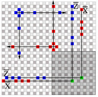
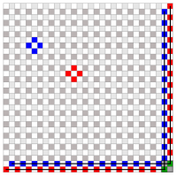
Figure 1: (Color online) Left: Two stabilizer generators (marked by arrows) and two pairs of anticommuting logical operators (marked by lines) of a $[[450,98,5]]$ code in Eq. (13) formed by circulant matrices $\mathcal{H}_{1}=\mathcal{H}_{2}$ corresponding to coefficients of the polynomial $h(x)=1+x+x^{3}+x^{7}$ (red – $X$ operators, blue – $Z$ operators, green – overlap of $Z$ and $X$ operators, dark and light gray – dual sublattices of physical qubits). All other stabilizer generators are obtained by shifts over the same sublattice with periodic boundaries. In the shaded region, each gray square uniquely corresponds to a different logical operator, thus $98$ encoded logical qubits. Right: same for the toric code $[[450,2,15]]$.

II.4 Hypergraph-product codes

Tillich and Zémor proposed a CSS construction which can be interpreted as a finite-rate generalization of toric codesTillich and Zemor (2009) and allows for LDPC constructions. For such codes, the generator matrix is constructed from a product of two hypergraphs, each corresponding to a parity check matrix of a classical binary code. The associated CSS code can be recast in a matrix form with the generators given byKovalev and Pryadko (2012)

$$\begin{array}[]{c}{\displaystyle G_{X}=(E_{2}\otimes\mathcal{H}_{1},\mathcal{H}_{2}\otimes E_{1}),}\\ {\displaystyle G_{Z}=(\mathcal{H}_{2}^{T}\otimes\widetilde{E}_{1},\widetilde{E}_{2}\otimes\mathcal{H}_{1}^{T}).}\end{array}$$ (13)

Here each sublattice block is constructed as a Kronecker product (denoted with “$\otimes$”) of two binary matrices $\mathcal{H}_{1}$ (dimensions $r_{1}\times n_{1}$) and $\mathcal{H}_{2}$ (dimensions $r_{2}\times n_{2}$), and $E_{i}$ and $\widetilde{E}_{i}$, $i=1,2$, are unit matrices of dimensions given by $r_{i}$ and $n_{i}$, respectively. The matrices $G_{X}$ and $G_{Z}$, respectively, have $r_{1}r_{2}$ and $n_{1}n_{2}$ rows (not all of the rows are necessarily linearly independent), and they both have $N\equiv r_{2}n_{1}+r_{1}n_{2}$ columns, which gives the block length of the quantum code. The commutativity condition $G_{X}G_{Z}^{T}=0$ is obviously satisfied by Eq. (13) since the Kronecker product obeys $(A\otimes B)(C\otimes D)=AC\otimes BD$.

The parameters $[[N,K,D]]$ of thus constructed quantum code are determined by those of the four classical codes which use the matrices $\mathcal{H}_{1}$, $\mathcal{H}_{2}$, $\mathcal{H}_{1}^{T}$, and $\mathcal{H}_{2}^{T}$ as the parity-check matrices. The corresponding parameters are introduced as

$$\mathcal{C}_{\mathcal{H}_{i}}=[n_{i},k_{i},d_{i}],\quad\mathcal{C}_{\mathcal{H}_{i}^{T}}=[{\widetilde{n}}_{i},\widetilde{k}_{i},\widetilde{d}_{i}],\quad i=1,2,$$ (14)

where we use the convention Tillich and Zemor (2009) that the distance $d_{i}(\widetilde{d}_{i})=\infty$ if $k_{i}(\widetilde{k}_{i})=0$. The matrices $\mathcal{H}_{i}$ are arbitrary, and are allowed to have linearly-dependent rows and/or columns. As a result, both $k_{i}=n_{i}-\mathop{\rm rank}\mathcal{H}_{i}$ and $\widetilde{k}_{i}=\widetilde{n}_{i}-\mathop{\rm rank}\mathcal{H}_{i}$ may be non-zero at the same time as the block length of the “transposed” code $\mathcal{C}_{\mathcal{H}_{i}^{T}}$ is given by the number of rows of $\mathcal{H}_{i}$, $\widetilde{n}_{i}=r_{i}$.

Specifically, for the hypergraph-product code (13), we have $N=r_{2}n_{1}+r_{1}n_{2}$, $K=2k_{1}k_{2}-k_{1}s_{2}-k_{2}s_{1}$ with $s_{i}=n_{i}-r_{i},\,i=1,2\,$ (Theorem 7 from Ref. Tillich and Zemor (2009)), while the distance $D$ satisfies the conditions $D\geq\min(d_{1},d_{2},\widetilde{d}_{1},\widetilde{d}_{2})$ (Theorem 9 from Ref. Tillich and Zemor (2009)), and two upper bounds (Lemma 10 from Ref. Tillich and Zemor (2009)): if $k_{1}>0$ and $\widetilde{k}_{2}>0$, then $D\leq d_{1}$; if $k_{2}>0$ and $\widetilde{k}_{1}>0$, then $D\leq d_{2}$.

A full-rank parity check matrix $\mathcal{H}_{1}$ of a binary code with parameters $\mathcal{C}_{\mathcal{H}_{1}}=[n_{1},k_{1},d_{1}]$ ($r_{1}=n_{1}-k_{1}$, $\widetilde{k}_{1}=0$) and $\mathcal{H}_{2}=\mathcal{H}_{1}^{T}$ define a quantum code with parameters $[[(n_{1}-k_{1})^{2}+n_{1}^{2},k_{1}^{2},d_{1}]]$Tillich and Zemor (2009). Furthermore, a family of finite-rate $(h,v)$-limited classical LDPC codes with asymptotically finite relative distance will correspond to a family of finite-rate $(v,h+v)$-limited quantum LDPC codes with the distance scaling as $D\propto\sqrt{N}$.

III Two-sublattice codes

The commutativity condition for QECCs in Eq. (7) puts a strong limitation on suitable parity check matrices. The problem becomes even more difficult when the additional requirement of LDPC structure is imposed. In particular, this strongly limits possible counting arguments for establishing bounds on code parameters. In such a setting, constructions based on some ansatz become very useful. In the following, we study several CSS constructions based on two sublattices corresponding to the columns of the binary matrices $A_{1}(B_{2}^{T})$ and $B_{1}(A_{2}^{T})$:

$$G_{X}=\left(A_{1},B_{1}\right),\quad G_{Z}=\left(B_{2}^{T},A_{2}^{T}\right),$$ (15)

where the matrices $A_{i}$, $B_{i}$, $i=1,2$, satisfy the condition $A_{1}B_{2}+B_{1}A_{2}=0$ (we assume binary linear algebra throughout this paper).

III.1 Two-sublattice CSS code from a generic stabilizer code

A large number of two-sublattice CSS codes (15) can be obtained from regular stabilizer codes by the following

Theorem 1.

For any quantum stabilizer code $[[N,K,D]]$ with the generator matrix

$$H=(A|B),$$ (16)

there is a reversible mapping to a two-sublattice quantum CSS code (15) with $A_{1}=A_{2}^{T}=A$, $B_{1}=B_{2}^{T}=B$ and the parameters $[[2N,2K,D^{\prime}]]$, where $D\leq D^{\prime}\leq 2D$.

Proof.

Explicitly, the generator matrices are

$$G_{X}=(A,B),\quad G_{Z}=(B,A).$$ (17)

The dimension of the code simply follows from Eqs. (9), (10), given that $\mathop{\rm rank}G_{X}=\mathop{\rm rank}G_{Z}=\mathop{\rm rank}H$. Any binary vector $\mathbf{e}=(\mathbf{a}|\mathbf{b})$ such that $A\mathbf{b}+B\mathbf{a}=0$ maps to a pair of double-size vectors $\mathbf{e}_{z}=(\mathbf{b},\mathbf{a})$, $\mathbf{e}_{x}=(\mathbf{a},\mathbf{b})$ which satisfy $G_{X}\mathbf{e}_{z}=0$, $G_{Z}\mathbf{e}_{x}=0$; the corresponding weights obey the inequality $\mathop{\rm wgt}\mathop{\rm OR}(\mathbf{a},\mathbf{b})\leq\mathop{\rm wgt}(\mathbf{a},\mathbf{b})\leq 2\mathop{\rm wgt}\mathop{\rm OR}(\mathbf{a},\mathbf{b})$, which ensures the conditions on the distance. It is easy to check that the reverse mapping also works. ∎

Note that an original code that exceeds the generic quantum Gilbert-Varshamov (GV) boundFeng and Ma (2004) is mapped to a CSS code that exceeds the version of the GV bound specific for such codesCalderbank and Shor (1996). Also, an original sparse code is mapped to a sparse code, with the same limit on the column weight, and row weight at most doubled. So, if one has a non-CSS code and wants to use one of the measurement techniques designed for such codes, this can be done by first constructing the corresponding CSS code.

We use the reverse version of this mapping in Sec. IV.8 to construct the non-CSS versions of hyperbicycle codes.

III.2 Generalized bicycle codes

Let us now start with two commuting square $n$ by $n$ binary matrices, $AB+BA=0$. Then, we can satisfy the general two-sublattice ansatz (15) by taking $A_{1}=A_{2}=A$, $B_{1}=B_{2}=B$, which gives

$$G_{X}=\left(A,B\right),\quad G_{Z}=\left(B^{T},A^{T}\right).$$ (18)

In particular, the commutativity is guaranteed for circulant matrices $A$ and $B$, which corresponds to a generalization of the bicycle codesMacKay et al. (2004), see Eq. (12). In this case, we map the linear combinations of rows in $G_{X}$ to a classical length-$n$ additive cyclic code over $\mathbb{F}_{4}$, where elements of the code are constructed from the generator matrix $\mathbb{G}=\omega A+B$. If the circulant matrices $A$ and $B$ are generated by the polynomials $f_{1}(x)$ and $f_{2}(x)$, respectively, the space of the additive code corresponding to the stabilizer is generated by the polynomial $g(x)=f_{1}(x)\omega+f_{2}(x)$ modulo $x^{n}-1$. That is, elements of the stabilizer are given by the coefficients of the polynomials $b(x)g(x)\mathop{\rm mod}(x^{n}-1)$, with arbitrary binary $b(x)$.

A canonical form of cyclic additive codes over $\mathbb{F}_{4}$ has been introduced in Ref. Calderbank et al., 1998, where Theorem 14 states that any cyclic additive code can be represented via two generators as $\left\langle\omega p(x)+q(x),r(x)\right\rangle$ $\mathop{\rm mod}(x^{n}-1)$ with $p(x)=\gcd[f_{1}(x),x^{n}-1]$, $r(x)=\gcd[(x^{n}-1)f_{2}(x)/p(x),x^{n}-1]$ and $\mathop{\rm deg}q(x)<\mathop{\rm deg}r(x)$ ($\gcd$ stands for the greatest common divisor). In this case the code dimensionality is $k=2n-\mathop{\rm deg}p(x)-\mathop{\rm deg}r(x)$. The special case of cyclic additive codes with a single generator has been analyzed in Ref. Kovalev et al. (2011) in which case the code dimensionality simplifies to $k=n-\mathop{\rm deg}p(x)$, which formally corresponds to $r(x)=x^{n}-1$. Note that, unlike the case of the usual quantum additive cyclic codesCalderbank et al. (1998); Kovalev et al. (2011), the mapping from Eq. (18) works for any circulant matrices $A$ and $B$; no additional commutativity condition is needed for the generator polynomials $p(x)$, $q(x)$, and $r(x)$. The parameters of thus obtained quantum codes are given by

Theorem 2.

The generalized bicycle codes in Eq. (18) have the block length $N=2n$, the number of encoded qubits $K=2\mathop{\rm deg}p(x)+2\mathop{\rm deg}r(x)-2n$ [$K=2\mathop{\rm deg}p(x)$ in the single generator case] and the distance exceeding or equal that of the classical code over $\mathbb{F}_{4}$ formed by codewords orthogonal to $\mathbb{G}$ with respect to the trace inner product.

Proof.

The code dimensionality immediately follows from the parameters of the canonical form of the code generated by $g(x)$. The orthogonal code contains the quantum code, hence the distance estimate. ∎

Note that the distance estimate in Theorem 2 is tight only for pure codes since a possibility for degeneracy is not taken into consideration.

Example 1.

Suppose a cyclic linear code $[n,k,d]$ over $\mathbb{F}_{4}$ with a generator polynomial $\varrho(x)$ that divides $x^{n}-1$ generates a code space $\mathbb{G}^{\perp}$. Then the parameters of the quantum CSS code in Eq. (18) are $[[2n,2n-4\mathop{\rm deg}\varrho(x),\geq d]]$. This construction is similar to non-CSS code construction from linear cyclic codes in Ref. Calderbank et al. (1998), except that here the dual code does not have to be self-orthogonal. For a cyclic $[30,25,4]$ code with $\varrho(x)=(1+x)^{2}(1+\omega x)(1+x+\omega x^{2})$ we obtain a quantum code $[[60,40,4]]$.

Example 2.

A CSS family of odd-distance rotated toric codes Kovalev and Pryadko (2012) is obtained for $f_{1}(x)=(1+x^{2t^{2}+1})$ and $f_{2}(x)=x(1+x^{2t^{2}-1})$, $t=1,2,\ldots$ by construction in Eq. (18). These codes have the parameters $[[2t^{2}+2(t+1)^{2},2,2t+1]]$. Explicitly, $[[10,2,3]]$, $[[26,2,5]]$, $[[50,2,7]]$, $[[82,2,9]]$, ….

The constructions in Theorems 1 and 2 [Eqs. (17) and (18) respectively] coincide for symmetric matrices, $A=A^{T}$, $B=B^{T}$. Then, starting with two palindromic polynomials $f_{i}(x)=x^{\mathop{\rm deg}f_{i}(x)}f_{i}(1/x)$, $i=1,2$, we can obtain non-CSS halved hyperbicycle codes in Eq. (16) by applying the reverse of Theorem 1 to the matrices $A$ and $B$ Kovalev and Pryadko (2012).

Example 3.

A non-CSS family of smallest odd-distance rotated toric codes Kovalev et al. (2011) is obtained for palindromic $f_{1}(x)=x^{t}(1+x^{2t^{2}+1})$ and $f_{2}(x)=x^{t+1}(1+x^{2t^{2}-1})$, $t=1,2,\ldots$ by construction in Eq. (16). These codes have the parameters $[[t^{2}+(t+1)^{2},1,2t+1]]$. Explicitly, $[[5,1,3]]$, $[[13,1,5]]$, $[[25,1,7]]$, $[[41,1,9]]$, ….

The codes in the last two examples exceed the lower bound in Theorem 2 due to degeneracy.

Code $1$.	$\begin{array}[]{l}A=\mathcal{H}_{1}\otimes E\otimes E+E\otimes\mathcal{H}_{1}\otimes E+E\otimes E\otimes\mathcal{H}_{1}\\ B=\mathcal{H}_{1}\otimes\mathcal{H}_{1}\otimes E+E\otimes\mathcal{H}_{1}\otimes\mathcal{H}_{1}+\mathcal{H}_{1}\otimes E\otimes\mathcal{H}_{1}\end{array}$
Code $2$.	$\begin{array}[]{l}A=\mathcal{H}_{1}\otimes E\otimes E+E\otimes\mathcal{H}_{1}\otimes E+E\otimes\mathcal{H}_{1}\otimes\mathcal{H}_{1}+\mathcal{H}_{1}\otimes E\otimes\mathcal{H}_{1}+\mathcal{H}_{1}\otimes\mathcal{H}_{1}\otimes\mathcal{H}_{1}\\ B=E\otimes E\otimes\mathcal{H}_{1}+\mathcal{H}_{1}\otimes\mathcal{H}_{1}\otimes E+E\otimes\mathcal{H}_{1}\otimes\mathcal{H}_{1}+\mathcal{H}_{1}\otimes E\otimes\mathcal{H}_{1}\end{array}$
Code $3$.	$\begin{array}[]{l}A=\mathcal{H}_{1}\otimes E\otimes E+E\otimes\mathcal{H}_{1}\otimes E+E\otimes\mathcal{H}_{1}\otimes\mathcal{H}_{1}+\mathcal{H}_{1}\otimes E\otimes\mathcal{H}_{1}+\mathcal{H}_{1}\otimes\mathcal{H}_{1}\otimes\mathcal{H}_{1}\\ B=\mathcal{H}_{1}\otimes E\otimes E+E\otimes\mathcal{H}_{1}\otimes E+E\otimes E\otimes\mathcal{H}_{1}+\mathcal{H}_{1}\otimes\mathcal{H}_{1}\otimes E+E\otimes\mathcal{H}_{1}\otimes\mathcal{H}_{1}+\mathcal{H}_{1}\otimes\mathcal{H}_{1}\otimes\mathcal{H}_{1}\end{array}$
Code $4$.	$\begin{array}[]{l}A=E\otimes\mathcal{H}_{1}\otimes\mathcal{H}_{1}+\mathcal{H}_{1}\otimes E\otimes\mathcal{H}_{1}+E\otimes\mathcal{H}_{1}\otimes E\\ B=\mathcal{H}_{1}\otimes E\otimes E+E\otimes E\otimes\mathcal{H}_{1}+E\otimes\mathcal{H}_{1}\otimes\mathcal{H}_{1}+\mathcal{H}_{1}\otimes\mathcal{H}_{1}\otimes\mathcal{H}_{1}\end{array}$

Table 1: Tensor-product two-sublattice representation of Haah’s codes corresponding to Eq. (15) where $\mathcal{H}_{1}$ is a circulant matrix corresponding to parity check polynomial $p(x)=1+x$ of a repetition code, $E$ is a unit matrix of the same dimensions with $\mathcal{H}_{1}$ and the summation is $\mathop{\rm mod}2$.

III.3 Tensor-product constructions and Haah’s codes

Further generalization of the bicycle-like construction in Eq. (18) can be achieved by combining tensor products with commuting (e.g., circulant) matrices. The most general form of two-sublattice tensor-product codes has the form:

$$\begin{array}[]{c}A=\sum_{i_{1}\ldots i_{k}}\mathcal{H}_{i_{1}}^{A}\otimes\ldots\otimes\mathcal{H}_{i_{k}}^{A},\\ B=\sum_{i_{1}\ldots i_{k}}\mathcal{H}_{i_{1}}^{B}\otimes\ldots\otimes\mathcal{H}_{i_{k}}^{B},\end{array}$$

where $\mathcal{H}_{i_{l}}^{A}$ and $\mathcal{H}_{i_{l}}^{B}$ are matching, pairwise-commuting binary square matrices (i.e., $\mathcal{H}_{i_{l}}^{A}\mathcal{H}_{j_{l}}^{B}+\mathcal{H}_{j_{l}}^{B}\mathcal{H}_{i_{l}}^{A}=0$). For circulant matrices $\mathcal{H}_{i_{l}}^{A}$ and $\mathcal{H}_{j_{l}}^{B}$ the commutativity is automatically satisfied.

Several examples of such codes are given by the Haah’s codesHaah (2011), which give examples of local codes in 3D without string logical operators, and may lead to realizations of self-correcting quantum memories. Such codes are defined on two sublattices and have exactly the tensor-product structure discussed here. In Table 1, we list four codes presented in Ref. Haah (2011). These codes are essentially constructed from a repetition code and it is straightforward to generalize this construction to arbitrary cyclic binary codes by using the corresponding binary circulant matrix $\mathcal{H}_{1}$. The commutativity of matrices $A$ and $B$ in Eq. (15) immediately follows.

A non-CSS generalization of construction in Table 1 can be achieved by using symmetric circulant matrices [see non-CSS construction in Eq. (16)].

IV CSS and non-CSS hyperbicycle codes

This section contains our most important results. We show that the families of hypergraph-product and generalized bicycle codes can be obtained as limiting cases of a larger family of hyperbicycle codes. The main advantage of this construction is that it gives a number of previously unreported families of quantum codes with tight bounds on, or even explicitly known distance. This includes many strongly degenerate LDPC codes with the distance much greater than the maximum weight of a stabilizer generator. In this section we discuss the construction of such codes, their parameters, and give examples.

IV.1 CSS hyperbicycle codes: construction

We define the hyperbicycle CSS codes as follows:

$$\begin{array}[]{c}{\displaystyle G_{X}={\displaystyle\Bigl{(}E_{b}\otimes{\textstyle\sum}_{i}I_{i}^{(\chi)}\otimes a_{i},\;{\textstyle\sum}_{i}b_{i}\otimes I_{i}^{(\chi)}\otimes E_{a}\Bigr{)}},}\\ {\displaystyle G_{Z}=\left({\textstyle\sum}_{i}b_{i}^{T}\otimes\widetilde{I}_{i}^{(\chi)}\otimes\widetilde{E}_{a},\;\widetilde{E}_{b}\otimes{\textstyle\sum_{i}}\widetilde{I}_{i}^{(\chi)}\otimes a_{i}^{T}\right).}\end{array}$$ (19)

Here we introduce two sets of binary matrices $a_{i}$ (dimensions $r_{1}\times n_{1}$, $i=0,\ldots,c-1$) and $b_{i}$ (dimensions $r_{2}\times n_{2}$, $i=0,\ldots,c-1$); $E_{a}$, $E_{b}$, $\widetilde{E}_{a}$ and $\widetilde{E}_{b}$ are unit matrices of dimensions given by $r_{1}$, $r_{2}$, $n_{1}$ and $n_{2}$, respectively. Matrices $I_{i}^{(\chi)}$ ($\widetilde{I}_{i}^{(\chi)}$) are permutation matrices given by a product of two permutation matrices, i.e. $I_{i}^{(\chi)}=S_{\chi}I_{i}$ ($\widetilde{I}_{i}^{(\chi)}=S_{\chi}^{T}I_{i}^{T}$) where $(I_{i})_{kj}=\delta_{j-k,i\mathop{\rm mod}c}$ is a circulant permutation matrix, $(S_{\chi})_{kj}=\delta_{j-k,(k-1)(\chi-1)\mathop{\rm mod}c}$ and the positive integers $c$ and $\chi$ are coprime . A version of this construction for $c=2$ and $\chi=1$ has been previously reported by us in Ref. Kovalev and Pryadko, 2012.

The matrices $G_{X}$ and $G_{Z}$, respectively, have $cr_{1}r_{2}$ and $cn_{1}n_{2}$ rows (not all of the rows are linearly independent), and they both have

$$N\equiv c(r_{1}n_{2}+r_{2}n_{1})$$ (20)

columns, which gives the block length of the quantum code. The commutativity condition $G_{X}G_{Z}^{T}=0$ is obviously satisfied by Eq. (19) since the permutation matrices commute with each other. Note that for $c=1$ and $\chi=1$ we recover the hypergraph-product codes in Eq. (13) and for $r_{i}=n_{i}=1$, $i=1,2$, (i.e., $a_{i}$ and $b_{i}$ given by binary numbers) we recover the generalized bicycle code construction in Eq. (18).

In order to characterize codes in Eq. (19) it is convenient to introduce the “tiled” binary matrices:

$$\begin{array}[]{c}\mathcal{H}_{1}={\textstyle\sum}_{i}I_{i}^{(\chi)}\otimes a_{i},\quad\mathcal{H}_{2}={\textstyle\sum}_{i}b_{i}\otimes I_{i}^{(\chi)},\\ \widetilde{\mathcal{H}}_{1}={\textstyle\sum}_{i}\widetilde{I}_{i}^{(\chi)}\otimes a_{i}^{T},\quad\widetilde{\mathcal{H}}_{2}={\textstyle\sum}_{i}b_{i}^{T}\otimes\widetilde{I}_{i}^{(\chi)}.\end{array}$$ (21)

For example, for $c=5$ and $\chi=2$ we have

$$\mathcal{H}_{1}=\left(\begin{array}[]{ccccc}a_{1}&a_{2}&a_{3}&a_{4}&a_{5}\\ a_{4}&a_{5}&a_{1}&a_{2}&a_{3}\\ a_{2}&a_{3}&a_{4}&a_{5}&a_{1}\\ a_{5}&a_{1}&a_{2}&a_{3}&a_{4}\\ a_{3}&a_{4}&a_{5}&a_{1}&a_{2}\end{array}\right);$$ (22)

note that the subsequent block rows are shifted by $\chi=2$ positions.

For the following discussion it is also useful to define auxiliary binary matrices:

$$\begin{array}[]{c}\mathcal{H}_{1}^{0}={\textstyle\sum}_{i}I_{i}\otimes a_{i},\quad\mathcal{H}_{2}^{0}={\textstyle\sum}_{i}b_{i}\otimes I_{i},\end{array}$$ (23)

where in terms of these matrices we can write:

$$\begin{array}[]{c}\mathcal{H}_{1}=S_{\chi}\otimes E_{a}\cdot\mathcal{H}_{1}^{0},\quad\mathcal{H}_{2}=E_{b}\otimes S_{\chi}\cdot\mathcal{H}_{2}^{0},\\ \widetilde{\mathcal{H}}_{1}=S_{\chi}^{T}\otimes E_{a}\cdot\mathcal{H}_{1}^{0T},\quad\widetilde{\mathcal{H}}_{2}=E_{b}\otimes S_{\chi}^{T}\cdot\mathcal{H}_{2}^{0T}.\end{array}$$ (24)

With this notation, it is clear that the generator matrices (19) correspond to the hypergraph generators (13), except that the identity matrices $E_{i}$, $\widetilde{E}_{i}$ are now reduced in size by a factor of $1/c$. The block length of the original hypergraph code with the present binary matrices (21) is

$$N_{\mathrm{orig}}=c^{2}(r_{1}n_{2}+r_{2}n_{1}).$$ (25)

In this sense, one can view the codes defined by Eq. (19) with $c>1$ as reduced hypergraph codes.

IV.2 CSS hyperbicycle codes: dimension

Just as for the hypergraph codes, the parameters of classical codes $\mathcal{C}_{\mathcal{H}_{i}}$ and $\mathcal{C}_{\widetilde{\mathcal{H}}_{i}}$ with parity check matrices $\mathcal{H}_{i}$ and $\widetilde{\mathcal{H}}_{i}$, respectively, contain information about the parameters of the quantum code in Eq. (19). We denote the distances of these binary codes as $d_{i}$ and $\widetilde{d}_{i}$, and their dimensions as $k_{i}$ and $\widetilde{k}_{i}$, $i=1,2$.

Regardless of the choice of the matrices $a_{i}$, $b_{i}$, the codes $\mathcal{C}_{\mathcal{H}_{i}}$ and $\mathcal{C}_{\widetilde{\mathcal{H}}_{i}}$ are quasicyclic, with the cycle of length equal the dimension $c$ of the cyclic permutation matrices $I_{\chi i}$ ($\widetilde{I}_{\chi i}$), $i=1,2$. Indeed, the corresponding block shifts merely lead to permutations of rows of the check matrices $\mathcal{H}_{i}$, $\widetilde{\mathcal{H}}_{i}$ [see Eq. (22)]. In order to define the dimension of the corresponding hyperbicycle codes with generators (19), we first classify the vectors in $\mathcal{C}_{\mathcal{H}_{i}}$ and $\mathcal{C}_{\widetilde{\mathcal{H}}_{i}}$ with respect to this circulant symmetry.

We start with the case of a binary cyclic code with block length $c$, with the generator polynomial $g(x)$, which divides $x^{c}-1$. [Polynomial algebra in this section is done modulo 2.] Any codeword corresponds to a polynomial $w(x)$ which contains $g(x)$ as a factor, and, therefore, every cyclotomic root of $g(x)$ is also a root of $w(x)$. However, the particular polynomial $w(x)=g(x)f(x)$ may also contain other factors of $x^{c}-1$ and thus have symmetry different from that of $g(x)$. We can define a linear space ${\cal C}^{(p)}$ of length-$c$ vectors corresponding to $w(x)$ with the exact symmetry of $g(x)$ where $p(x)\equiv(x^{c}-1)/g(x)$ by defining the equivalence $w_{1}(x)\equiv w_{2}(x)$ for a given $g(x)$ as $f_{1}=f_{2}\mathop{\rm mod}p^{\prime}(x)$ for all $p^{\prime}(x)$ such that $p^{\prime}(x)\neq p(x)$ is a factor of $p(x)$. The same equivalence can be also defined modulo greatest common divisor (gcd) of all such polynomials $p^{\prime}(x)$. In terms of the corresponding check polynomial $p(x)$, the dimension $k_{0}^{(p)}$ of thus defined space ${\cal C}^{(p)}$ is zero unless $p(x)$ is a non-zero power of an irreducible polynomial $p_{\alpha}(x)$, in which case $k_{0}^{(p)}=\mathop{\rm deg}p_{\alpha}(x)$.

For the quasicyclic code $\mathcal{C}_{\mathcal{H}_{1}}$ with the first check matrix in Eq. (21), the vector $\mathbf{w}$ is in the symmetry class of $p(x)$, where $p(x)$ divides $x^{c}-1$, if $\mathbf{w}$ satisfies the condition $[p(I_{1})\otimes E_{a}]\,\mathbf{w}=0$ and is not a member of such a symmetry class of any factor of $p(x)$. For each polynomial $p(x)$, the l.h.s. in these equations is a sum of cyclic shifts of the vector $\mathbf{w}$ corresponding to each non-zero coefficient of $p(x)$. We denote the dimension of the subcode of $\mathcal{C}_{\mathcal{H}_{1}}$ with all vectors in the symmetry class of $p(x)$ as $k_{1}^{(p)}$. The symmetry implies that $k_{1}^{(p)}$ must contain the dimension $k_{0}^{(p)}$ introduced in the previous paragraph as a factor, and, in particular, $k_{1}^{(p)}$ must be zero whenever $k_{0}^{(p)}$ is zero. A convenient basis of ${\cal C}_{{\cal H}_{1}}^{(p)}$ can be constructed using the following

Lemma 1.

Any vector of the subcode ${\cal C}_{{\cal H}_{1}}^{(p)}$ can be chosen in the form

$$\mathbf{w}=\sum_{i=0}^{k_{0}^{(p)}-1}I_{i}\mathbf{g}\otimes\bm{\alpha}_{i},$$ (26)

where the vector $\mathbf{g}$ corresponds to the generating polynomial $g(x)\equiv(x^{c}-1)/p(x)$; the vectors $(I_{s}\otimes E_{a})\mathbf{w}$, $0\leq s<k_{0}^{(p)}$, are linearly independent.

Proof.

Any vector of the subcode ${\cal C}_{{\cal H}_{1}}^{(p)}$ can be expanded in the form $\bm{\omega}_{i}^{(p)}\otimes\mathbf{e}_{i}$, where $\mathbf{e}_{i}$ are all distinct weight-one vectors, and $\bm{\omega}_{i}^{(p)}$ are vectors from ${\cal C}^{(p)}$. Generally, any vector $\bm{\omega}\in{\cal C}^{(p)}$ can be written as a sum of shifts of the vector $\mathbf{g}$, $\sum_{s=0}^{k_{0}^{(p)}-1}I_{s}\mathbf{g}$; we obtain Eq. (26) by rearranging the summations. Linear independence follows from the symmetry of the vectors $\bm{\omega}_{i}^{(p)}\in{\cal C}^{(p)}$. ∎

Note that, in addition to the symmetric vectors, the code $\mathcal{C}_{\mathcal{H}_{1}}$ may contain vectors with no special symmetry with respect to the discussed block shifts. We will formally assign these to the check polynomial $p(x)=x^{c}-1$, and define $k_{0}^{(x^{c}-1)}\equiv 1$.

For the vectors of the code $\mathcal{C}_{\mathcal{H}_{2}}$ with the second check matrix in Eq. (21), the condition to be in the symmetry class of $p(x)$ reads $[E_{b}\otimes p(I_{1})]\mathbf{w}=0$ while $[E_{b}\otimes p^{\prime}(I_{1})]\mathbf{w}\neq 0$ for all $p^{\prime}(x)\neq p(x)$ that divide $p(x)$. We denote the dimension of the corresponding subcode as $k_{2}^{(p)}$. The same classification can be done for codes $\mathcal{C}_{\widetilde{\mathcal{H}}_{i}}$ with the transposed check matrices; the corresponding dimensions are ${\widetilde{k}}_{i}^{(p)}$, $i=1,2$.

The introduced symmetry classification is in the heart of the following

Lemma 2.

A vector $\bm{\upsilon}$ that belongs to both $\mathcal{C}_{E_{b}\otimes\mathcal{H}_{1}}$ and $\mathcal{C}_{\mathcal{H}_{2}\otimes E_{a}}$ must be in the same symmetry class $p(x)$ with respect to both codes ${\cal H}_{1}$ and ${\cal H}_{2}$, including the no-symmetry case $p(x)=x^{c}-1$. Any such vector can be generally expanded in terms of

$$\bm{\upsilon}_{\alpha,\beta}=\sum_{i,j=0}^{k_{0}^{(p)}-1}\bm{\beta}_{i}\otimes I_{i+j}\mathbf{g}\otimes\bm{\alpha}_{j},$$ (27)

where $\sum_{i}\bm{\beta}_{i}\otimes I_{i}\mathbf{g}\in{\cal C}_{{\cal H}_{2}}^{(p)}$ and $\sum_{i}I_{i}\mathbf{g}\otimes\bm{\alpha}_{i}\in{\cal C}_{{\cal H}_{1}}^{(p)}$ and $\mathbf{g}$ corresponds to the polynomial $g(x)\equiv(x^{c}-1)/p(x)$.

Proof.

The parameter $\chi$ does not enter this discussion since it corresponds to permutations of rows in matrices ${\cal H}_{1}^{0}$ and ${\cal H}_{2}^{0}$. That the symmetry must be the same becomes evident if we write the most general expansion

$$\bm{\upsilon}=\sum_{ij}\mathbf{e}_{i}^{2}\otimes\bm{\gamma}_{ij}\otimes\mathbf{e}_{j}^{1},$$ (28)

where $\bm{\gamma}_{ij}$ are length-$c$ vectors and $\mathbf{e}_{i}^{1(2)}$ are distinct weight-1 vectors. Indeed, the condition to be in the symmetry class of $p(x)$ is the same for both codes: $[E_{b}\otimes p(I_{1})\otimes E_{a}]\bm{\upsilon}=0$ for $p(x)$ itself but not for any of its factors; thus $\bm{\gamma}_{ij}$ must be in ${\cal C}^{(p)}$. The expansion (27) follows from Lemma 1. ∎

We can now count linearly-independent rows in the generator matrices:

Lemma 3.

The numbers of linearly independent rows in matrices (19) are

$$\mathop{\rm rank}G_{X} = r_{1}r_{2}c-\sum_{l}\widetilde{k}_{1}^{(p_{l})}\widetilde{k}_{2}^{(p_{l})}/k_{0}^{(p_{l})},$$

$$\mathop{\rm rank}G_{Z} = n_{1}n_{2}c-\sum_{l}k_{1}^{(p_{l})}k_{2}^{(p_{l})}/k_{0}^{(p_{l})},$$ (29)

where $p_{l}(x)$ are all binary factors of $x^{c}-1$ such that $k_{0}^{(p_{l})}\neq 0$, including $x^{c}-1$ itself.

Proof.

We first count linearly-dependent rows in $G_{Z}$. Notice that the equations $\bm{\upsilon}^{T}\cdot(E_{b}\otimes\widetilde{\mathcal{H}}_{1})=0$ and $\bm{\upsilon}^{T}\cdot(\widetilde{\mathcal{H}}_{2}\otimes E_{a})=0$ are both satisfied for $\bm{\upsilon}$ in Eq. (27) [Lemma 2]. Each pair $(\bm{\alpha},\bm{\beta})$ generates $k_{0}^{(p)}$ linearly-independent vectors, same as each of them generates for the corresponding subcodes ${\cal C}_{{\cal H}_{i}}^{(p)}$, $i=1,2$, respectively. Thus there are exactly $k_{1}^{(p)}k_{2}^{(p)}/k_{0}^{(p)}$ linearly-independent vectors corresponding to every $p(x)$ with non-empty ${\cal C}^{(p)}$. Such vectors have to be complemented with the pairs of vectors of no symmetry (if any) which formally correspond to $p(x)=x^{c}-1$ and $k_{0}^{(p)}=1$. According to Lemma 2 these are all possible solutions, which gives $\mathop{\rm rank}G_{Z}$ in Eq. (29). We obtain $\mathop{\rm rank}G_{X}$ by substituting the parameters of the codes with the parity check matrices $\widetilde{\mathcal{H}}_{1}$, $\widetilde{\mathcal{H}}_{2}$. ∎

We finally obtain

Theorem 3.

A quantum CSS code with generators (19) encodes

$$K=2\sum_{l}k_{1}^{(p_{l})}k_{2}^{(p_{l})}/k_{0}^{(p_{l})}-k_{1}s_{2}-k_{2}s_{1}$$ (30)

qubits, where $p_{l}(x)$ are all binary factors of $x^{c}-1$ such that $k_{0}^{(p_{l})}\neq 0$, including $x^{c}-1$ itself, and $s_{i}=n_{i}-r_{i}$, $i=1,2$.

Proof.

The number of encoded qubits $K$ can be deduced from Lemma 3 using the relation

$$k_{i}^{(p)}-\widetilde{k}_{i}^{(p)}=s_{i}k_{0}^{(p)},\;i=1,2.$$ (31)

The latter follows from the fact that the rank of a matrix does not change under transposition (and also under permutations of rows and columns, e.g., as needed to transform $\mathcal{H}_{i}$ into $\widetilde{\mathcal{H}}_{i}$). Specifically, restricting the action of matrices $\mathcal{H}_{i}$ and $\widetilde{\mathcal{H}}_{i}$ to subspace $\mathcal{C}^{(p)}$, we obtain reduced mutually transposed matrices of dimensions given by $r_{i}k_{0}^{(p)}\times n_{i}k_{0}^{(p)}$ and $n_{i}k_{0}^{(p)}\times r_{i}k_{0}^{(p)}$, which immediately gives Eq. (31). ∎

By construction, any $k_{i}^{(p)}$ may only be non-zero if the corresponding $k_{i}>0$, $i=1,2$. Then, Eq. (30) gives

Consequence 4.

A quantum CSS code with generators (19) can only have $K>0$ if at least one of the binary codes with the parity check matrices (21) is non-empty.

IV.3 CSS hyperbicycle codes: general distance bounds

Theorem 5.

The minimum distance of the code with generators (19) satisfies the lower bound

$$D\geq\lfloor d/c\rfloor,\quad d\equiv\min(d_{1},d_{2},\widetilde{d}_{1},\widetilde{d}_{2}).$$ (32)

Proof.

Consider a vector $\mathbf{u}$ such that $G_{X}\cdot\mathbf{u}=0$. We construct a reduced quantum code in the form (19), with the same $c$, by keeping only those columns of the matrices $a_{i}$, $b_{i}$ that are involved in the product $G_{X}\cdot\mathbf{u}$. This way, for every non-zero bit of $\mathbf{u}$, one of the reduced matrices $\mathcal{H}_{1}^{\prime}$, $\mathcal{H}_{2}^{\prime}$ [see Eq. (21)] may get $c$ columns, so that these matrices have no more than $c\mathop{\rm wgt}(\mathbf{u})$ columns. If we take $\mathop{\rm wgt}(\mathbf{u})<\lfloor d/c\rfloor$, according to Consequence 4, the reduced code encodes no qubits, thus the corresponding reduced $\mathbf{u}^{\prime}$, $G_{X}^{\prime}\cdot\mathbf{u}^{\prime}=0$, has to be a linear combination of the rows of $G_{Z}^{\prime}$. The rows of $G_{Z}^{\prime}$ are a subset of those of $G_{Z}$, with some all-zero columns removed; thus the full vector $\mathbf{u}$ is also a linear combination of the rows of $G_{Z}$. Similarly, a vector $\mathbf{v}$ such that $G_{Z}\cdot\mathbf{v}=0$ and $\mathop{\rm wgt}(\mathbf{v})<\left\lfloor d/c\right\rfloor$, is a linear combination of rows of $G_{X}$. ∎

Let us introduce the minimum distances $d_{i}^{(p)}$ corresponding to the subset of the vectors of the code $\mathcal{C}_{\mathcal{H}_{i}}$ which contain one of the vectors with the exact symmetry of $p(x)$,

$$d_{i}^{(p)}=\min\{\mathop{\rm wgt}(\mathbf{a}+\mathbf{b})|\mathbf{0}\neq\mathbf{a}\in\mathcal{C}_{\mathcal{H}_{i}}^{(p)},\;\mathbf{b}\in\mathcal{C}_{\mathcal{H}_{i}}\setminus\mathcal{C}_{\mathcal{H}_{i}}^{(p)}\}.$$ (33)

Evidently, thus introduced distances satisfy

$$d_{i}^{(p)}\geq d_{i},\quad\min_{l}d_{i}^{(p_{l})}=d_{i},\;i=1,2;$$ (34)

the minimum is taken over all $p_{l}(x)$ as in Theorem 3. We will also introduce the distances $\widetilde{d}_{i}^{(p)}$ corresponding to the matrices $\widetilde{\mathcal{H}}_{i}$, $i=1,2$.

The upper bound on the distance of the code with generators (19) is formulated in terms of thus introduced subset-distances ${d}_{i}^{(p)}$, $\widetilde{d}_{i}^{(p)}$, $i=1,2$:

Theorem 6.

For every $p(x)$, a binary factor of $x^{c}-1$ such that $k_{1}^{(p)}>0$ and $\widetilde{k}_{2}^{(p)}>0$, the minimum distance $D$ of the code with generators (19) satisfies $D\leq\min(d_{1}^{(p)},\widetilde{d}_{2}^{(p)})$. Similarly, when $k_{2}^{(p)}>0$ and $\widetilde{k}_{1}^{(p)}>0$, we have $D\leq\min(d_{2}^{(p)},\widetilde{d}_{1}^{(p)})$.

Proof.

Given $k_{1}^{(p)}>0$, consider vector $\mathbf{u}\equiv(\mathbf{e}\otimes\mathbf{c},0)$, where $\mathbf{c}\in\mathcal{C}_{\mathcal{H}_{1}}^{(p)}$ and $\mathop{\rm wgt}(\mathbf{e})=1$. As long as $\widetilde{k}_{2}^{(p)}>0$, we can always select such $\mathbf{e}$ that $\mathbf{u}$ is not a linear combination or rows of $G_{Z}$, which would indicate that $D\leq\mathop{\rm wgt}(\mathbf{c})$.

Indeed, by construction, vector $\mathbf{c}$ can be written in the form (26); let us pick a bit $s$ which is not identically zero in all $\alpha_{i}$ and construct a vector [cf. Eq. (27)]

$$\mathbf{u}^{(p),s}=(\underbrace{\mathbf{e}\otimes\sum_{i}\alpha_{is}I_{i}\mathbf{g}}\otimes\mathbf{e}_{s}^{1},0).$$ (35)

Taking all $r_{2}$ different vectors $\mathbf{e}$ and all $k_{0}^{(p)}$ linearly-independent translations [Lemma 1], we obtain the vector space [as indicated in Eq. (35) with a brace] isomorphic to that on which the subcode $\mathcal{C}_{\widetilde{\mathcal{H}}_{2}}^{(p)}$ operates. On the other hand, there are only $r_{2}k_{0}^{(p)}-\widetilde{k}_{2}^{(p)}$ linearly-independent combinations of rows of the matrix $\widetilde{\mathcal{H}}_{2}$ restricted to the subspace $\mathcal{C}^{(p)}$. Since $\widetilde{k}_{2}^{(p)}>0$, at least one of vectors $\mathbf{u}^{(p),s}$ is linearly independent of the rows of the matrix $\widetilde{\mathcal{H}}_{2}$ restricted to the subspace $\mathcal{C}^{(p)}$.

Now, we can construct such a vector $\mathbf{u}$ for every $\mathbf{c}$ from the set in Eq. (34), which proves $D\leq d_{1}^{(p)}$. The other bounds in the Theorem can be obtained from this one by considering isomorphic codes [e.g., interchanging $\widetilde{\mathcal{H}}_{2}$ and $\mathcal{H}_{1}$, and also $\mathcal{H}_{1}$ and $\mathcal{H}_{2}$]. ∎

The meaning of the condition on $p(x)$ in Theorem 6 can be elucidated if we rewrite the number of encoded qubits (30) with the help of identity (31),

$$K=\sum_{l}k_{1}^{(p_{l})}\widetilde{k}_{2}^{(p_{l})}/k_{0}^{(p_{l})}+\sum_{l}k_{2}^{(p_{l})}\widetilde{k}_{1}^{(p_{l})}/k_{0}^{(p_{l})}.$$ (36)

Obviously, every term in Eq. (36) giving a non-zero contribution to $K$, also gives an upper bound on the minimum distance of the quantum code.

IV.4 Codes with finite rate and distance scaling as square root of block length

Here we show that the family of hyperbicycle codes contain $(v,h+v)$-limited LDPC codes with the distance $D\propto\sqrt{N}$ that are distinct from the hypergraph product codes. Let us start with a random $(h,v)$-regular parity check matrix of a classical LDPC code, where $h<v$. By removing linearly dependent rows, we can form full-rank $(h,v)$-limited parity check matrix $a_{1}$ that, along with $b_{j}=a_{1}^{T}$ ($j\neq 1$ and $\chi$ are arbitrary, in case when $j=1$ and $\chi=1$ we recover the hypergraph-product codes), we use in Eq. (19) in order to construct the hyperbicycle code where only one term in each summation in Eq. (19) is taken. The rate of the classical code defined by the parity check matrix $a_{1}$ is bounded from below, i.e. $R_{\mathrm{c}}\equiv k_{\mathrm{c}}/n_{\mathrm{c}}\geq 1-h/v$. With high probability at large $n_{\mathrm{c}}$, the classical code will also have the relative distance in excess of some finite number $\delta_{\mathrm{c}}$Litsyn and Shevelev (2002). If the classical LDPC code defined by $a_{1}$ has parameters $[n_{1},k_{1},d_{1}]$ then, according to Theorem 3, 6 and 5, the quantum code will have parameters $[[c(n_{1}-k_{1})^{2}+cn_{1}^{2},ck_{1}^{2},\geq d_{1}/c]]$. It follows that a finite rate $(h,v)$-limited classical LDPC code (defined by the parity check matrix $a_{1}$) with finite relative distance (we expect the subset relative distance in  (34) to be finite as well) will correspond to a finite rate $(v,h+v)$-limited quantum LDPC code with the distance $D\propto\sqrt{N}$.

IV.5 Codes with repeated codewords

In some cases the distance of the hyperbicycle codes is larger than the lower bound in Theorem 5. In this section we consider the special case of square matrices $a_{i}$, $b_{i}$ ($r_{i}=n_{i}$), with the additional restriction that the codes ${\cal C}_{{\cal H}_{i}}$, ${\cal C}_{\widetilde{\mathcal{H}}_{i}}$ are non-empty ($k_{i}=\widetilde{k}_{i}>0$) and contain only fully-symmetric vectors in the symmetry class of $p(x)=1+x$. The results we proved so far give the parameters of such codes summarized by (see also Theorem 3 in Ref. Kovalev and Pryadko (2012))

Consequence 7.

Suppose $a_{i}$ and $b_{i}$ in Eq. (21) are such that $k_{i}^{(1+x)}=k_{i}>0$ and $r_{i}=n_{i}$. Then the CSS code with generators (19) has the block length $N=2cn_{1}n_{2}$, encodes $K=2k_{1}k_{2}$ qubits, and has the minimum distance $D$ limited by $\lfloor d/c\rfloor\leq D\leq d$, $d\equiv\min(d_{1},d_{2},\widetilde{d}_{1},\widetilde{d}_{2})$.

Proof.

By assumption, all vectors in the codes ${\cal C}_{{\cal H}_{i}}$, $i=1,2$, are in the symmetry class of $p(x)=1+x$, which corresponds to $k_{0}^{(p)}=1$ and block-symmetric vectors in the form

$$\mathbf{w}_{1}=\mathbf{g}\otimes\bm{\alpha},\quad\mathbf{w}_{2}=\bm{\beta}\otimes\mathbf{g},$$ (37)

respectively, with $\mathbf{g}=(1,\ldots,1)$ [see Eq. (26)]. The number of encoded qubits $K$ immediately follows from Theorem 3, the block length $N$ from Eq. (20), and the lower bound on the distance from Theorem 5. Furthermore, with all vectors in the binary codes having the same symmetry, the upper bound in Theorem 6 is just $D\leq d$. ∎

At this point we notice that the proof of the lower bound $\lfloor d/c\rfloor$ on the distance in Theorem 5 implies that there may be uncorrectable errors of the form $\sum_{s}(\bm{\beta}_{s}\otimes{\bf g}_{s}\otimes\bm{\beta}_{s}^{\prime},\bm{\alpha}_{s}^{\prime}\otimes{\bf g}_{s}\otimes\bm{\alpha}_{s})$, where all $\mathbf{g}_{s}$ have $\mathop{\rm wgt}(\mathbf{g}_{s})=1$. On the other hand, if we were to consider only fully-symmetric vectors, with $\mathbf{g}_{s}=\mathbf{g}=(1,\ldots,1)$, the factor of $1/c$ would be unnecessary. We formulate this result as

Lemma 4.

A symmetric vector $\mathbf{u}=(\mathbf{w}_{1},\mathbf{w}_{2})$, $\mathbf{w}_{i}=\sum_{s}\bm{\beta}_{s}^{i}\otimes\mathbf{g}\otimes\bm{\alpha}_{s}^{i}$ with $\mathbf{g}=(1,\ldots,1)$, $i=1,2$, that satisfies $G_{X}\mathbf{u}=0$ and is linearly independent from the rows of $G_{Z}$, has sublattice weights $\mathop{\rm wgt}(\mathbf{w}_{i})$ either zero or $\geq d$.

Let us first consider the case $c=2$ (then $\chi$ must be equal to $1$); we previously formulated the sufficient conditions to increased lower distance bound as Theorem 3 in Ref. Kovalev and Pryadko (2012) which was given without a proof.

Theorem 8.

Suppose $c=2$, $a_{i}$ and $b_{i}$ in Eq. (21) are such that $k_{i}^{(1+x)}=k_{i}>0$, $r_{i}=n_{i}$ and binary codes with generator matrices $\sum a_{i}$, $\sum a_{i}^{T}$, $\sum b_{i}$ and $\sum b_{i}^{T}$ have distances at least $2$. Then the CSS quantum code with generators Eq. (19) has parameters $[[4n_{1}n_{2},2k_{1}k_{2},d]]$, where $d=\min(d_{1},d_{2},\widetilde{d}_{1},\widetilde{d}_{2})$.

Proof.

In addition to what is stated in Consequence 7, we only need to prove that $d$ is also the lower bound on the distance. To this end, notice that any vector $\mathbf{u}$ such that $G_{X}\mathbf{u}=0$ can be decomposed as the sum of an “actual” solution plus degeneracy, $\mathbf{u}^{(1+x)}+\bm{\gamma}^{T}G_{Z}$, where $\mathbf{u}^{(1+x)}\equiv(\mathbf{w}_{1},\mathbf{w}_{2})$ is a block-symmetric vector satisfying the conditions of Lemma 4 and linearly-independent from the rows of $G_{Z}$. This decomposition can be verified by comparing $K$ with the number of linearly-independent solutions in the form (35), as well as those on the other sublattice. First, let us assume $\mathop{\rm wgt}(\mathbf{w}_{1})>0$ and therefore $\mathop{\rm wgt}(\mathbf{w}_{1})\geq d$. We can rewrite the corresponding decomposition as $\mathbf{w}_{1}=\sum_{s}\bm{\beta}_{s}\otimes\mathbf{g}\otimes\mathbf{e}_{s}^{1}$, where $\mathbf{g}\equiv(1,1)$, each $\mathbf{e}_{s}^{1}$ has length $n_{1}$ and $\mathop{\rm wgt}(\mathbf{e}_{s}^{1})=1$, with the non-zero element in the position $s$; there must be at least $d/2$ non-zero vectors $\bm{\beta}_{s}$. The full solution including the degeneracy can be formally written as $\sum_{s}\mathbf{w}_{1s}^{\prime}\otimes\mathbf{e}_{s}^{1}$, where

$$\mathbf{w}_{1s}^{\prime}\equiv\bm{\beta}_{s}\otimes\mathbf{g}+\bm{\gamma}^{\prime}_{s}\otimes(1,0)+\bm{\gamma}^{\prime\prime}_{s}\otimes(1,0),$$ (38)

where the sum of the last two vectors is a linear combination of rows of $\widetilde{\mathcal{H}}_{2}$. The key to the proof is the observation that $\bm{\gamma}^{\prime}_{s}+\bm{\gamma}^{\prime\prime}_{s}$ is a linear combination of rows of $a_{0}^{T}+a_{1}^{T}$, and therefore is in the binary code generated by $\sum_{s}a_{s}$; by condition the corresponding weight is either zero or $\geq 2$. Without limiting generality we can drop the case $\bm{\gamma}^{\prime}_{s}=\bm{\gamma}^{\prime\prime}_{s}\neq\mathbf{0}$ which corresponds to a symmetric vector and can be included as a part of $\mathbf{u}^{(1+x)}$. We are left with the trivial $\bm{\gamma}^{\prime}_{s}=\bm{\gamma}^{\prime\prime}_{s}=0$, in which case $\mathbf{w}_{1s}^{\prime}=\bm{\beta}_{s}\otimes(1,1)$ remains unchanged; otherwise $\bm{\gamma}^{\prime}_{s}\neq\bm{\gamma}^{\prime\prime}_{s}$, in which case the weight of the modified $\mathbf{w}_{1s}^{\prime}$ can be lower bounded by that of the sum of the components corresponding to $(1,0)$ and $(0,1)$,

$$\mathop{\rm wgt}(\mathbf{w}_{1s}^{\prime})\geq\mathop{\rm wgt}(\bm{\gamma}_{s}^{\prime}+\bm{\gamma}_{s}^{\prime\prime})\geq 2;$$ (39)

with at least $d/2$ such terms the total weight is $d$ or greater. The same arguments can be repeated in the case $\mathop{\rm wgt}(\mathbf{w}_{2})\neq 0$, as well as for the space orthogonal to $G_{X}$. Overall, this proves the lower bound $D\geq d$; combined with the upper bound we get $D=d$. ∎

Theorem 9.

Suppose $c$ is even, $a_{i}$ and $b_{i}$ in Eq. (21) are such that $k_{i}^{(1+x)}=k_{i}$, $r_{i}=n_{i}$ and binary codes with generator matrices $\sum a_{i}$, $\sum a_{i}^{T}$, $\sum b_{i}$ and $\sum b_{i}^{T}$ have distance at least $2$. Then the quantum code in Eq. (19) has parameters $[[2n_{1}n_{2}c,2k_{1}k_{2},D]]$, where $(2/c)d\leq D\leq d$ and $d\equiv\min(d_{1},d_{2},\widetilde{d}_{1},\widetilde{d}_{2})$.

Proof.

The proof is similar to the proof of Theorem 8, except that now vectors $\mathbf{w}_{1s}^{\prime}$ are defined by the analog of Eq. (38) which has $\mathbf{g}=(1,\ldots,1)$ with $c$ components and more terms with $\gamma_{s}^{(j)}$ in the r.h.s., $j=1,\ldots,c$. We need to show that a non-zero $\mathbf{w}_{1s}^{\prime}$ has $\mathop{\rm wgt}(\mathbf{w}_{1s}^{\prime})\geq 2$, which ensures that the minimum distance of the code is at least $2d/c$.

With $c>2$ and even, after the summation over all possible shifts of the vector $\mathbf{w}_{1s}^{\prime}$ with respect to the block structure the symmetric term disappears, and we obtain the inequality $c\mathop{\rm wgt}(\mathbf{w}_{1s}^{\prime})\geq c\mathop{\rm wgt}(\bm{\gamma}^{1}_{s}+\bm{\gamma}^{2}_{s}+\ldots+\bm{\gamma}^{c}_{s})$. The sum in the r.h.s. is a linear combination of rows of $\sum a_{i}^{T}$; by assumption, it’s weight is either $\geq 2$ or zero. The only non-trivial situation corresponds to the latter case with some $\bm{\gamma}_{s}^{\ell_{1}}\neq 0$. For the sum to be zero, either there is an even number $m$ of identical vectors $\bm{\gamma}_{s}^{\ell_{1}}=\bm{\gamma}_{s}^{\ell_{2}}=\ldots=\bm{\gamma}_{s}^{\ell_{m}}$, with $m<c$ and all indices different [this situation results in $\mathop{\rm wgt}(\mathbf{w}_{1s}^{\prime})\geq(c-m)\geq 2$ since both $m$ and $c$ are even and $\bm{\beta}_{s}\neq\mathbf{0}$], or there are at least two pairs of unequal vectors $\bm{\gamma}_{s}^{\ell_{1}}\neq\bm{\gamma}_{s}^{\ell_{2}}$ and $\bm{\gamma}_{s}^{\ell_{3}}\neq\bm{\gamma}_{s}^{\ell_{4}}$, with $\bm{\gamma}_{s}^{\ell_{2}}\neq\bm{\gamma}_{s}^{\ell_{4}}$, which also gives $\mathop{\rm wgt}(\mathbf{w}_{1s}^{\prime})\geq 2$. ∎

In order to obtain codes with repeated structure (see Fig. 2), one can start with two cyclic LDPC codes with block lengths $n_{i}$, $i=1,2$, and the check polynomials $h_{i}(x)$ that divide $x^{n_{i}}-1$. The polynomials $h_{i}(x)$ will also divide $x^{cn_{i}}-1$, thus the corresponding circulant parity-check matrix $\mathcal{H}_{i}$ of dimensions $cn_{i}\times cn_{i}$ will lead to a code with repeated structure satisfying Theorem 9 since the corresponding generator polynomial is $g_{i}(x)=(x^{(c-1)n_{i}}+x^{(c-2)n_{i}}+\ldots+1)\,(x^{n_{i}}+1)/h_{i}(x)$, $i=1,2$.

Example 4.

Suppose we use the polynomial $h(x)$ corresponding to the shortened Reed-Muller cyclic code with parameters $[2^{m}-1,m+1,2^{m-1}-1]$ in order to construct circulant matrices $\mathcal{H}_{1}=\mathcal{H}_{2}$ of dimensions $2(2^{m}-1)\times 2(2^{m}-1)$. According to Theorem 9, a code in Eq. (19) with $c=2$ and $\chi=1$ will have parameters $[[4(2^{m}-1)^{2},2(m+1)^{2},2(2^{m-1}-1)]]$. This family leads to weight limited LDPC codes and up to $m=11$ there is always a choice of polynomial $h(x)$ of weight $4$ which leads to quantum LDPC code with stabilizer generators of weight $8$.

Example 5.

Given two “small” cyclic codes $[n_{i},k_{i},d_{i}]$ with check polynomials $h_{i}(x)$, $i=1,2$, we can construct a $c=1$ hypergraph-product quantum code with the parameters $[[2n_{1}n_{2},2k_{1}k_{2},d]]$, $d=\min(d_{1},d_{2})$, a repeated even-$c$ code with the parameters $[[2cn_{1}n_{2},2k_{1}k_{2},D]]$, $2d\leq D\leq cd$, or a hypergraph-product code $[[2c^{2}n_{1}n_{2},2k_{1}k_{2},dc]]$ using the “large” cyclic codes with the same check polynomials and the block lengths $cn_{i}$.

Note that in this Example the code rate goes down compared to the hypergraph-product code constructed from the “small” cyclic codes and goes up compared to the hypergraph-product code constructed from the “large” cyclic codes.

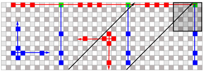
Figure 2: (Color online) Same as Fig. 1 for the $[[294,18,4\leq D\leq 12]]$ code in Eq. (19) formed by circulant matrices $\mathcal{H}_{1}=\mathcal{H}_{2}$ corresponding to coefficients of the polynomial $h(x)=1+x+x^{3}$ with $c=3$ and $\chi=1$. Two stabilizer generators are marked by red and blue arrows, respectively, and two anticommuting logical operators are marked by red and blue lines, respectively. All other stabilizer generators are obtained by shifts over the same sublattice with periodicity in the horizontal direction and shifted periodicity (shown by arrows) in the vertical direction. In the shaded region, each gray square uniquely corresponds to a different logical operator, thus $18$ encoded logical qubits. One can observe the tripling of the logical operators, thus the overlap (green square) is also repeated three times.

IV.6 Planar qubit layout of hyperbicycle codes and encoding

The stabilizer generators corresponding to Eq. (19) can be graphically represented on two rectangular regions corresponding to two sublattices. In case, when matrices $\mathcal{H}_{1}$ and $\mathcal{H}_{2}$ are square, the rectangular regions of sublattices have the same dimensions and can be drawn together with parameters $c$ and $\chi$ corresponding to the number of square blocks and boundary shift, respectively, see, e.g., Fig. 3. Furthermore, in some cases, we can represent logical operators by line-like operators with a possibility of using this layout for encoding.

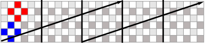
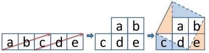
Figure 3: (Color online) Upper plot: visualization of a $[[90,2,9]]$ toric (hyperbicycle) code in Eq. (19) formed by circulant matrices $\mathcal{H}_{1}$ and $\mathcal{H}_{2}$ corresponding to coefficients of the polynomial $h(x)=1+x$, $c=5$ and $\chi=3$. The boundaries are periodic in the horizontal direction and shifted (as shown by arrows) in the horizontal direction by $\chi=3$ blocks. Lower plot: general block construction leading to rotated periodic boundaries of hyperbicycle codes for $c=5$ blocks and for the shift $\chi=3$. This corresponds to $t=1$ case of the infinite series of block constructions with $c=t^{2}+(t+1)^{2}$ and $\chi=2t+1$, e.g., in case of toric code we get $[[2n^{2}c,2,n\chi]]$ for any integer $n>1$.

We start by considering the case $c=1$ and $\chi=1$ corresponding to the hypergraph-product codes. The stabilizer generators for the quantum code in Eq. (13) can be graphically represented by two (dotted) lines living on different sublattices with the dots (red and blue squares in Fig. 1 marked by arrows) placed in the positions corresponding to $1$s in rows of the binary matrices $\mathcal{H}_{1}$, $\mathcal{H}_{2}$, $\widetilde{\mathcal{H}}_{1}=\mathcal{H}_{1}^{T}$ and $\widetilde{\mathcal{H}}_{2}=\mathcal{H}_{2}^{T}$. For cyclic codes, e.g., in Fig. 1, the relative position of dots stays the same and we can translate each stabilizer generator over the corresponding sublattice. In general, the form of stabilizer generators is position dependent and the peculiar two-line structure (see Fig. 1) ensures commutativity. The logical operators $\overline{X}_{j}$, $\overline{Z}_{j}$, $j=1,...,k$ can be chosen among the rows of the matrices $\overline{\mathcal{X}}_{1}=(\mathcal{H}_{2}^{T\perp}\otimes\widetilde{E}_{1},0)$, $\overline{\mathcal{X}}_{2}=(0,\widetilde{E}_{2}\otimes\mathcal{H}_{1}^{T\perp})$ and $\overline{\mathcal{Z}}_{1}=(E_{2}\otimes\mathcal{H}_{1}^{\perp},0)$, $\overline{\mathcal{Z}}_{2}=(0,\mathcal{H}_{2}^{\perp}\otimes E_{1})$ where the index corresponds to the sublattice number on which the logical operator lives, $\perp$ stands for the orthogonal space $\mathop{\rm mod}2$ and matrices $\mathcal{H}_{1}^{\perp}$, $\mathcal{H}_{2}^{\perp}$, $\mathcal{H}_{1}^{T}{}^{\perp}$ and $\mathcal{H}_{2}^{T}{}^{\perp}$ are in a row echelon form. By row and column permutations on matrices $\mathcal{H}_{1}$, $\mathcal{H}_{2}$ it is convenient to reduce matrices $\mathcal{H}_{1}^{\perp}$, $\mathcal{H}_{2}^{\perp}$, $\mathcal{H}_{1}^{T}{}^{\perp}$ and $\mathcal{H}_{2}^{T}{}^{\perp}$ to the form with an identity matrix on the right. In such a case, the logical operators can be represented by vertical and horizontal (dotted) lines that have only one non-zero element in the region of the size $k_{1}\times\tilde{k}_{2}$ for the first sublattice and of the size $\tilde{k}_{1}\times k_{2}$ for the second sublattice (shaded region in Fig. 1) resulting in $k=k_{1}\tilde{k}_{2}+\tilde{k}_{1}k_{2}$ logical qubits. Thus, for such a representation, each physical qubit in the region of size $k_{1}\tilde{k}_{2}+\tilde{k}_{1}k_{2}$ (shaded region in Fig. 1) overlaps with only one logical qubit and can be used for encoding. Note that in general the two sublattices cannot be drawn together as they will have different dimensions for non-square matrices $\mathcal{H}_{1}$ and $\mathcal{H}_{2}$. In such a case, the sublattices can be represented by two different rectangular regions and the stabilizer generators have one line per sublattice.

The hyperbicycle construction in Eq. (19) for arbitrary $c$ and $\chi$ has a block structure of several rectangular regions stitched together with one of the periodic boundaries being shifted by $\chi$ blocks (see Fig. 3). The stabilizer generators can be graphically represented by two (dotted) lines with the dots (red and blue squares in Fig. 4) placed in the positions corresponding to $1$s in rows of the binary matrices $\mathcal{H}_{1}$, $\mathcal{H}_{2}$, $\widetilde{\mathcal{H}}_{1}$ and $\widetilde{\mathcal{H}}_{2}$. For cyclic codes, e.g., in Fig. 4, the relative position of dots stays the same and we can translate the stabilizer generator with (shifted) periodic boundaries. Just like for the hypergraph product codes, the form of stabilizer generators is position dependent in case of non-cyclic codes. In general, codes with $c>1$ have complicated structure of logical operators. Nevertheless, in a specific case of CSS codes when $c$ is odd and $k_{i}^{(1+x)}=k_{i}$ (see Theorem 3), we can recover the form of logical operators $\overline{X}_{j}$, $\overline{Z}_{j}$, $j=1,...,k$ obtained in $c=1$ case where the operators can be chosen among the rows of the matrices $\overline{\mathcal{X}}_{1}=(\widetilde{\mathcal{H}}_{2}^{\perp}\otimes\widetilde{E}_{1},0)$, $\overline{\mathcal{X}}_{2}=(0,\widetilde{E}_{2}\otimes\widetilde{\mathcal{H}}_{1}^{\perp})$ and $\overline{\mathcal{Z}}_{1}=(E_{2}\otimes\mathcal{H}_{1}^{\perp},0)$, $\overline{\mathcal{Z}}_{2}=(0,\mathcal{H}_{2}^{\perp}\otimes E_{1})$. The only difference is that the logical operators are now repeated $c$ times which can lead to codes with increased distance (see Fig. 2).

Example 6.

A CSS $[[900,50,14]]$ hyperbicycle code is obtained with circulant $\mathcal{H}_{1}=\mathcal{H}_{1}^{0}$ corresponding to the polynomial $h(x)=(1+x+x^{3}+x^{5})$, $n_{i}=15$, $c=2$, $\chi=1$, and $b_{i}=a_{i}$.

Note that one-to-one correspondence between a set of physical qubits (shaded region in Figs. 1 and 2) and logical qubits can be used for encoding.

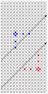
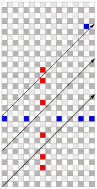
Figure 4: (Color online) Same as Fig. 1. Left: $X$ and $Z$ stabilizer generators for the CSS hyperbicycle code $[[900,50,14]]$ formed by circulant matrices corresponding to coefficients of a polynomial $h(x)=1+x+x^{3}+x^{5}$ and $c=2$, $\chi=1$. Right: a single stabilizer generator of a $[[289,81,5]]$ non-CSS hyperbicycle code in Eq. (16) formed by circulant matrices corresponding to coefficients of a polynomial $h(x)=1+x+x^{3}+x^{6}+x^{8}+x^{9}$ and $c=1$. The division into two sublattices is impossible and all other stabilizer generators are obtained by shifts over the light and dark gray qubits with periodicity in the vertical direction and shifted periodicity (shown by arrows) in the horizontal direction.

IV.7 Codes from two circulant matrices

The hyperbicycle construction in Eq. (19) can employ the known families of cyclic codes when matrices $\mathcal{H}_{1}^{0}$ and $\mathcal{H}_{2}^{0}$ (after additional permutations that change the order in the Kronecker product) in Eq. (23) are circulant. Note that any circulant matrix will have the block form of Eq. (23). As was mentioned in the previous section, for circulant matrices $\mathcal{H}_{1}^{0}$ and $\mathcal{H}_{2}^{0}$ the stabilizer generators are translationally invariant with (shifted) periodic boundaries.

The choice of $\chi\neq 1$ can lead to codes with increased distance. This can be best seen on the example with the toric code (Fig. 3) where by rearranging the surface of the code we can bring it into a new layout with proper periodic but rotated boundaries. Then the Manhattan distance (defined on blocks, e.g., $3$ in Fig. 3) between the boundaries will actually determine the distance of the code. The largest distance can be expected for squares thus by defining the boundary angle as $(t,t+h)$ we arrive at codes with $c=t^{2}+(t+h)^{2}$, $\chi=2t+h$ and the Manhattan distance equal to $\chi$. Compared to the general distance bound in Theorem 5 for toric codes we achieve the distance: $D=\chi d/c$. As the following examples confirm, numerically we see that $\chi>1$ can produce codes exceeding the distance bound in Theorem 5, often saturating the upper distance bound in Theorem 6.

Example 7.

A CSS family of rotated toric codes is obtained when $\mathcal{H}_{1}^{0}$ corresponds to the polynomial $h(x)=(1+x)$ (for $\mathcal{H}_{2}^{0}$ we use $b_{i}=a_{i}$), $c=t^{2}+(t+1)^{2}$, $\chi=2t+1$, $t=1,2,\ldots$. By construction in Eq. (19) we obtain codes with parameters $[[2n^{2}c,2,n\chi]]$. Explicitly for $n=2$ we obtain $[[40,2,6]]$, $[[104,2,10]]$…, and for $n=3$ $[[90,2,9]]$, $[[234,2,15]]$ ….

Example 8.

A $[[90,8,8]]$ CSS hyperbicycle code is obtained when $\mathcal{H}_{1}^{0}$ corresponds to the classical cyclic code $[15,4,8]$ with the generator polynomial $g(x)=(1+x^{3}+x^{4})$ (for $\mathcal{H}_{2}^{0}$ we use $b_{i}=a_{i}$), $c=5$ and $\chi=3$.

Example 9.

A $[[90,10,7]]$ CSS hyperbicycle code is obtained when $\mathcal{H}_{1}^{0}$ corresponds to the classical cyclic code $[15,5,7]$ with the check polynomial $h(x)=(1+x+x^{3}+x^{5})$ (for $\mathcal{H}_{2}^{0}$ we use $b_{i}=a_{i}$), $c=5$ and $\chi=3$.

Example 10.

A $[[126,8,10]]$ CSS hyperbicycle code is obtained when $\mathcal{H}_{1}^{0}$ corresponds to the classical cyclic code $[21,5,10]$ with the check polynomial $h(x)=(1+x+x^{5})$ (for $\mathcal{H}_{1}^{0}$ we use $b_{i}=a_{i}$), $c=7$ and $\chi=3$. Same construction with $\chi=1$ results in the code $[[126,14,6]]$.

Example 11.

Same construction starting with the classical cyclic code $[30,8,8]$ with the check polynomial $h(x)=(1+x^{2}+x^{8})$, $c=10$ and $\chi=3$ gives a code $[[180,16,8]]$, while $\chi=1$ gives $[[180,16,6]]$ with a smaller distance.

Example 12.

Same construction starting with the classical cyclic code $[[30,8,8]]$ corresponding to the check polynomial $h(x)=(1+x^{2}+x^{8})$ with $c=15$ and $\chi=2$ gives a $[[120,32,4]]$ CSS hyperbicycle code; $\chi=1$ gives a code $[[120,32,2]]$.

Note that in many cases the code rate goes up compared to the hypergraph-product code constructed from the same cyclic codes while the construction from the “small” cyclic codes is not possible (cf. Example 5).

IV.8 Non-CSS versions of hyperbicycle codes

We observe that when $\mathcal{H}_{1}=\widetilde{\mathcal{H}}_{1}$ and $\mathcal{H}_{2}=\widetilde{\mathcal{H}}_{2}$, the construction in Eqs. (19) can be mapped to non-CSS codes in Eq. (16) that in many cases have the same distance but half the number of encoded and physical qubits. In particular, this happens when $\chi=1$ and matrices $\mathcal{H}_{1}$ and $\mathcal{H}_{2}$ are symmetric. By non-CSS hyperbicycle codes we then mean a result of the mapping in Theorem 1 of the code in Eq. (19). The dimensions of such codes can be readily found by applying Theorem 3 where $s_{1}=s_{2}=0$.

Theorem 10.

A quantum non-CSS code constructed from matrices (24) such that $\mathcal{H}_{1}=\widetilde{\mathcal{H}}_{1}$ and $\mathcal{H}_{2}=\widetilde{\mathcal{H}}_{2}$ and the stabilizer generator matrix

$$G=(E_{b}\otimes\mathcal{H}_{1}|\mathcal{H}_{2}\otimes E_{a}),$$ (40)

encodes $K=\sum_{l}k_{1}^{(p_{l})}k_{2}^{(p_{l})}/k_{0}^{(p_{l})}$ logical qubits into $N=cn_{1}n_{2}$ physical qubits, where $p_{l}(x)$ are all binary factors of $x^{c}-1$ such that $k_{0}^{(p_{l})}\neq 0$, including $x^{c}-1$ itself. The distance of such a code is bounded by $D\geq\lfloor d/c\rfloor,\quad d\equiv\min(d_{1},d_{2})$ (same notations as in Theorem 5).

Proof.

The distance bound follows from the proof of Theorem 5 given the fact that any code word of the original quantum code has to have support on at least one of the sublattices with weight exceeding $\lfloor d/c\rfloor$.∎

Theorem 11.

Suppose $c$ is even, $a_{i}$ and $b_{i}$ in Eq. (21) are such that $k_{i}^{(1+x)}=k_{i}$, $r_{i}=n_{i}$ and binary codes with generator matrices $\sum a_{i}$ and $\sum b_{i}$ have distance at least $2$. Then quantum non-CSS code with generators in Eq. (19) that have been reduced by construction in Eq. (16) has parameters $[[n_{1}n_{2}c,k_{1}k_{2},\geq(2/c)d]]$ where $d=\min(d_{1},d_{2})$.

Proof.

This distance bound follows from the proof of Theorem 8 given the fact that any code word of the original quantum code has to have support on at least one of the sublattices with weight exceeding $(2/c)d$.∎

Finally, we would like to mention that the upper distance bound in Theorem 6 also applies to non-CSS hyperbicycle codes since by construction this bound involves only one sublattice.

For $\chi=1$ we can use palindromic check polynomials $h(x)$, i.e. $x^{\mathop{\rm deg}h(x)}h(1/x)=h(x)$, such that $cn-\mathop{\rm deg}h(x)$ is even, in order to construct symmetric circulant matrices $\mathcal{H}_{i}$ from the polynomial $x^{[cn-\mathop{\rm deg}h(x)]/2}h(x)$.

Example 13.

A $[[289,81,5]]$ non-CSS hyperbicycle code (see Fig. 4) is obtained from Eqs. (16) and  (19) using circulant matrices $\mathcal{H}_{1}=\mathcal{H}_{2}$ corresponding to coefficients of a palindromic polynomial $h(x)=1+x+x^{3}+x^{6}+x^{8}+x^{9}$ where $c=1$ and $\chi=1$.

V Conclusions

We described a large family of hyperbicycle codes that includes as subclasses the best of the known LDPC codes. The construction allows for explicit upper and lower bounds on the code distance. We also described new LDPC code families with finite rates and distances scaling as a square root of block length. Our discussion is accompanied with geometrical interpretations of the hyperbicycle codes which can facilitate design and applications of such codes. The construction is particularly important for designing LDPC codes with relatively small block lengths which is important since the original hypergraph product codes have relatively poor parameters at small block lengths.

Another advantage of hyperbicycle construction is that it can be based on a pair of very well studied classical cyclic codes. This leads to codes with good parameters up to limited but relatively large block lengths (in general, cyclic codes with asymptotic rates below one have poor asymptotic parameters). The planar layout of thus constructed quantum codes possess translational invariance of stabilizer generators which may simplify the implementation (see e.g. Ref. De and Pryadko (2012)).

Although the quantum LDPC codes discussed in this work have been shown to possess a finite noise threshold Kovalev and Pryadko (2012), it is yet to be seen whether there are good decoders for such codes. It may well happen that the relation between hyperbicycle and bicycle codes can lead to better decoding for the former as the latter are known for their good decoding properties.

Even though the lower distance bounds presented in this paper are in some cases inferior compared to the hypergraph-product codes, we do not expect that this will have a significant effect on the value of the noise threshold as the distance still scales as a square root of the block length while the LDPC structure of the stabilizer generators is preserved Kovalev and Pryadko (2012). Given that, we expect that one can encode more qubits into hyperbicycle codes compared to hypergraph product codes without affecting the threshold.

Our results notwithstanding, there are several open questions in regard to the hyperbicycle codes. In particular, it would be interesting to establish conditions under which the hyperbicycle codes reach the upper distance bound. Furthermore, the case when the block shift $\chi$ and the number of blocks $c$ are commensurate has not been analyzed. It would also be interesting to explore the exact relation between the hyperbicycle codes and the CSS codes constructed over higher alphabets Andriyanova et al. (2012); Kasai et al. (2012).

References

- Vandersypen et al. (2000) L. M. K. Vandersypen, M. Steffen, G. Breyta, C. S. Yannoni, R. Cleve, and I. L. Chuang, Phys. Rev. Lett. 85, 5452 (2000), URL http://link.aps.org/abstract/PRL/v85/p5452.
- Vandersypen et al. (2001) L. M. K. Vandersypen, M. Steffen, G. Breyta, C. S. Yannoni, M. H. Sherwood, and I. L. Chuang, Nature 414, 883 (2001), URL http://dx.doi.org/10.1038/414883a.
- Chiaverini et al. (2004) J. Chiaverini, D. Leibfried, T. Schaetz, M. D. Barrett, R. B. Blakestad, J. Britton, W. M. Itano, J. D. Jost, E. Knill, C. Langer, et al., Nature 432, 602 (2004), URL http://dx.doi.org/10.1038/nature03074.
- Martinis (2009) J. M. Martinis, Quantum Information Processing 8, 81 (2009), URL http://dx.doi.org/10.1007/s11128-009-0105-1.
- Shor (1995) P. W. Shor, Phys. Rev. A 52, R2493 (1995), URL http://link.aps.org/abstract/PRA/v52/pR2493.
- Knill and Laflamme (1997) E. Knill and R. Laflamme, Phys. Rev. A 55, 900 (1997), URL http://dx.doi.org/10.1103/PhysRevA.55.900.
- Bennett et al. (1996) C. Bennett, D. DiVincenzo, J. Smolin, and W. Wootters, Phys. Rev. A 54, 3824 (1996), URL http://dx.doi.org/10.1103/PhysRevA.54.3824.
- Knill et al. (1998) E. Knill, R. Laflamme, and W. H. Zurek, Science 279, 342 (1998), URL http://www.sciencemag.org/cgi/content/abstract/279/5349/342.
- Rahn et al. (2002) B. Rahn, A. C. Doherty, and H. Mabuchi, Phys. Rev. A 66, 032304 (2002), URL http://dx.doi.org/10.1103/PhysRevA.66.032304.
- Dennis et al. (2002) E. Dennis, A. Kitaev, A. Landahl, and J. Preskill, Journal of Mathematical Physics 43, 4452 (2002), URL http://link.aip.org/link/?JMP/43/4452/1.
- Steane (2003) A. M. Steane, Phys. Rev. A 68, 042322 (2003), URL http://dx.doi.org/10.1103/PhysRevA.68.042322.
- Fowler et al. (2004a) A. G. Fowler, C. D. Hill, and L. C. L. Hollenberg, Phys. Rev. A 69, 042314 (2004a), URL http://link.aps.org/abstract/PRA/v69/e042314.
- Fowler et al. (2004b) A. G. Fowler, S. J. Devitt, and L. C. L. Hollenberg, Quant. Info. Comput. 4, 237 (2004b), quant-ph/0402196, URL http://arxiv.org/abs/quant-ph/0402196.
- Fowler (2005) A. G. Fowler (2005), arXiv:quant-ph/0506126, URL http://arxiv.org/abs/quant-ph/0506126.
- Knill (2005a) E. Knill, Nature 434, 39 (2005a), URL http://dx.doi.org/10.1038/nature03350.
- Knill (2005b) E. Knill, Phys. Rev. A 71, 042322 (2005b), URL http://dx.doi.org/10.1103/PhysRevA.71.042322.
- Raussendorf and Harrington (2007) R. Raussendorf and J. Harrington, Phys. Rev. Lett. 98, 190504 (2007), URL http://link.aps.org/abstract/PRL/v98/e190504.
- Postol (2001) M. S. Postol (2001), unpublished, eprint arXiv:quant-ph/0108131v1, URL http://arxiv.org/abs/quant-ph/0108131.
- MacKay et al. (2004) D. MacKay, G. Mitchison, and P. McFadden, Information Theory, IEEE Transactions on 50, 2315 (2004).
- Kitaev (2003) A. Y. Kitaev, Ann. Phys. 303, 2 (2003), URL http://arxiv.org/abs/quant-ph/9707021.
- Bombin and Martin-Delgado (2007) H. Bombin and M. A. Martin-Delgado, Phys. Rev. A 76, 012305 (2007).
- Freedman et al. (2002) M. Freedman, D. Meyer, and F. Luo, in Computational Mathematics (Chapman and Hall/CRC, 2002), URL http://dx.doi.org/10.1201/9781420035377.ch12.
- Tillich and Zemor (2009) J.-P. Tillich and G. Zemor, in Information Theory, 2009. ISIT 2009. IEEE International Symposium on (2009), pp. 799 –803.
- Kovalev and Pryadko (2012) A. A. Kovalev and L. P. Pryadko (2012), eprint quant-ph/arXiv:1208.2317.
- Aly (2008) S. Aly, in Global Telecommunications Conference, 2008. IEEE GLOBECOM 2008. IEEE (2008), pp. 1 –5.
- Farinholt (2012) J. Farinholt (2012), eprint quant-ph/arXiv:1207.0732.
- Couvreur et al. (2012) A. Couvreur, N. Delfosse, and G. Zémor (2012), eprint cs/arXiv:1206.2656.
- Calderbank et al. (1998) A. R. Calderbank, E. M. Rains, P. M. Shor, and N. J. A. Sloane, IEEE Trans. Inf. Th. 44, 1369 (1998), URL http://dx.doi.org/10.1109/18.681315.
- Gottesman (1997) D. Gottesman, Ph.D. thesis, Caltech (1997), URL http://arxiv.org/abs/quant-ph/9705052.
- Calderbank and Shor (1996) A. R. Calderbank and P. W. Shor, Phys. Rev. A 54, 1098 (1996).
- Poulin and Chung (2008) D. Poulin and Y. Chung, Quant. Info. and Comp. 8, 987 (2008), URL http://arxiv.org/,0801.1241.
- Kovalev and Pryadko (2012) A. A. Kovalev and L. P. Pryadko, in Information Theory Proceedings (ISIT), 2012 IEEE International Symposium on (2012), pp. 348 –352.
- Feng and Ma (2004) K. Feng and Z. Ma, Information Theory, IEEE Transactions on 50, 3323 (2004).
- Kovalev et al. (2011) A. A. Kovalev, I. Dumer, and L. P. Pryadko, Phys. Rev. A 84, 062319 (2011).
- Haah (2011) J. Haah, Phys. Rev. A 83, 042330 (2011), URL http://link.aps.org/doi/10.1103/PhysRevA.83.042330.
- Litsyn and Shevelev (2002) S. Litsyn and V. Shevelev, Information Theory, IEEE Transactions on 48, 887 (2002).
- De and Pryadko (2012) A. De and L. P. Pryadko (2012), eprint quant-ph/arXiv:1209.2764.
- Andriyanova et al. (2012) I. Andriyanova, D. Maurice, and J. Tillich, in Information Theory Proceedings (ISIT), 2012 IEEE International Symposium on (2012), pp. 343 –347.
- Kasai et al. (2012) K. Kasai, M. Hagiwara, H. Imai, and K. Sakaniwa, Information Theory, IEEE Transactions on 58, 1223 (2012).